Lepton-proton two-photon exchange with improved soft-photon approximation including proton’s structure effects in HB$\chi$PT

Abstract

We present an improved evaluation of the two-photon exchange correction to the unpolarized lepton-proton elastic scattering process at very low-energies relevant to the MUSE experiment, where only the dominant intermediate elastic proton is considered. We employ the framework of heavy baryon chiral perturbation theory and invoke the soft-photon approximation in order to reduce the intricate 4-point loop-integrals into simpler 3-point loop-integrals. In the present work, we adopt a more robust methodology compared to an earlier work along the same lines for analytically evaluating the loop-integrations, and incorporate important corrections at next-to-next-to-leading order. These include the proton’s structure effects which renormalize the proton-photon interaction vertices and the proton’s propagator. Finally, our results allow a model-independent estimation of the charge asymmetry for the scattering of unpolarized massive leptons and anti-leptons.

I Introduction

The two-photon exchange (TPE) contribution in the context of unpolarized lepton-proton ($\ell$-p, where $\ell\equiv e^{\pm},\mu^{\pm}$) elastic scattering refers to the quantum mechanical effect in which two virtual photons are exchanged between a lepton and a target proton. This process constitutes an important higher-order radiative correction to the leading one-photon exchange (OPE) mechanism, which dominates the low-energy scattering process. The advent of the form factor discrepancy Jones:1999rz ; Perdrisat:2006hj ; Punjabi:2015bba ; Puckett:2010 and the proton’s radius puzzle Pohl:2010zza ; Pohl:2013 ; Antognini:1900ns ; Bernauer:2014 ; Carlson:2015 ; Bernauer:2020ont has generated renewed interest in the scientific community concerning the TPE mechanism, due to its potential role in explaining both discrepancies, simultaneously. Significant efforts have been invested in the last two decades to estimate the TPE contributions in elastic lepton- and anti-lepton-proton scattering both experimentally and theoretically. Earlier analyses of radiative corrections to $\ell$-p scattering included the TPE merely to cancel the infrared (IR) divergence arising from the so-called charge-odd soft-photon bremsstrahlung counterparts (namely, from the interference process between a lepton and a proton each emitting a single soft-photon), focusing mainly on high-energy kinematics Arrington:2003 ; Guichon:2003 ; Blunden:2003sp ; Rekalo:2004wa ; Blunden:2005ew ; Carlson:2007sp ; Arrington:2011 ). However, persuaded by a host of ongoing/planned high-precision experiments targeted at low-energy kinematics (e.g., see Ref. Gao:2021sml for a recent review), the current demand, therefore, requires improved reliability of modeling and precision evaluation of the TPE intermediate hadronic states and their interaction. This motivated an entire gamut of recent rigorous TPE analyses pertinent to low-momentum transfer kinematics employing different perturbative and non-perturbative techniques Kivel:2012vs ; Lorenz:2014yda ; Tomalak:2014sva ; Tomalak:2014dja ; Tomalak:2015aoa ; Tomalak:2015hva ; Tomalak:2016vbf ; Tomalak:2017npu ; Koshchii:2017dzr ; Tomalak:2018jak ; Bucoveanu:2018soy ; Talukdar:2019dko ; Peset:2021iul ; Talukdar:2020aui ; Kaiser:2022pso ; Guo:2022kfo ; Engel:2023arz ; Cao:2021nhm ; Choudhary:2023rsz .

One such approach is to systematically analyze the non-perturbative dynamics of hadrons in the model-independent framework of a chiral effective field theory (EFT). In EFT the hadrons are effectively treated as elementary degrees of freedom with a low-energy perturbative expansion for typical momenta far below a well-defined breakdown scale. The isospin SU(2) version of the heavy baryon chiral perturbation theory (HBChPT) is one such EFT. It provides a systematic computational framework to investigate the low-energy structure and dynamics of mesons and nucleons, and it also allows a study of their responses to external weak and electromagnetic currents Gasser:1982ap ; Jenkins:1990jv ; Bernard:1992qa ; Ecker:1994pi ; Bernard:1995dp . However, the applicability is limited to typical momentum scales not much larger than the pion mass and far below the chiral symmetric breaking scale $\Lambda_{\chi}\simeq 1$ GeV/c. In addition, HBChPT entails a chiral expansion scheme in powers of the inverse nucleon mass $M$, i.e., ${\mathcal{Q}}/M$ where ${\mathcal{Q}}$ is the generic momentum scale. In our analysis, $\mathcal{Q}$ will correspond to the typical magnitude of the 4-momentum transfer $|Q|=\sqrt{-Q^{2}}$ for the elastic $t$-channel scattering process. The framework is ideally suited for a gauge-invariant estimation of the non-perturbative recoil-radiative corrections relevant to low-energy $\ell$-p scattering. Recently, the corresponding TPE radiative corrections were estimated up-to-and-including next-to-leading order (NLO), both in the context of the soft photon approximation (SPA) by Talukdar et al. Talukdar:2019dko ; Talukdar:2020aui , as well as the exact TPE evaluation in Choudhary et al. Choudhary:2023rsz , all at low-$Q^{2}$ kinematics relevant to the ongoing MUSE experiment at PSI Gilman:2013eiv . In particular, in the SPA-based approach Talukdar:2019dko , one of the two photon propagator momenta is set to zero, following the method outlined in the work of Mo and Tsai Mo:1968cg . This is a well-known technique widely adopted in works on radiative corrections for simplifying the evaluation of complicated 4-point TPE loop-integrals (see e.g., Refs. Koshchii:2017dzr ; Bucoveanu:2018soy ; Maximon:1969nw ; Maximon:2000hm ; Vanderhaeghen:2000ws ). Furthermore, we note the following two features regarding the SPA analysis of Talukdar et al Talukdar:2019dko that deserve some introspection:

• As only the dominant real (or dispersive) part of the low-energy TPE contribution is relevant for evaluating the unpolarized elastic scattering cross-section, certain simplifying approximations were adopted in evaluating the TPE loops, such as dropping the complex $\pm i\epsilon$ parts from the propagators within the TPE loops. Such an approximation could, however, be a source of unwarranted systematics that should be avoided to achieve better precision.

• The infrared (IR) divergences which were isolated via dimensional regularization (DR) led to a contribution to the cross-section proportional to

  $$-\frac{2}{D-4}-\gamma_{E}+\ln\left(\frac{4\pi\mu^{2}}{-Q^{2}}\right)\,,$$

  where $D>4$ is the analytically continued space-time dimension, $\gamma_{E}=0.577216...$ is the Euler-Mascheroni constant and $\mu$ is an arbitrary subtraction scale. Since the subtraction scheme adopted to eliminate such singularities contains $Q^{2}$-dependent terms, certain dynamical contributions from the residual finite part of the TPE could be lost. Therefore, it is more appropriate to choose a subtraction scheme for the TPE analysis that is $Q^{2}$-independent, for example, proportional to $\ln(m^{2}_{l})$, namely,

  $$-\frac{2}{D-4}-\gamma_{E}+\ln\left(\frac{4\pi\mu^{2}}{m^{2}_{l}}\right)\,,$$

  where $m_{l}$ is the lepton mass.

The purpose of the current work is to improve upon the SPA results of Talukdar et al. Talukdar:2019dko (a) by including some of the dominant TPE corrections of next-to-next-to-leading order (NNLO) that also include effects due to the proton’s radius and anomalous magnetic moment at the level of one-loop accuracy, and (b) by refining some of the approximations used in that study by employing a more rigorous treatment of the loop-integrations with an improved IR-subtraction scheme. In addition, we shall present the corresponding charge asymmetry results in SPA by including the soft-photon bremsstrahlung contributions at NLO as was considered in the work of Ref. Talukdar:2020aui . The paper is organized as follows. In Sec. II, we present the specifics of our modus operandi in regard to the low-energy EFT framework, along with the kinematical settings used in our analytical calculations. The analytical expressions for the various orders of the fractional TPE corrections up to NNLO are evaluated in this section. We then utilize our SPA-based TPE results up to NLO in this section, along with the rest of the NLO radiative corrections results obtained earlier by Talukdar et al. Talukdar:2020aui , to obtain an estimate of the charge asymmetry observable (between lepton-proton and anti-lepton-proton scatterings) in Sec. III. Finally, in Sec. IV, we discuss our numerical results in the context of low-energy kinematics relevant to the proposed MUSE experiment kinematical region. We also provide an appendix where we collect the analytical expressions of all relevant loop-integrations used to obtain our results.

II Effective Lagrangian and Kinematics of TPE

The relevant parts of the effective $\pi N$ chiral Lagrangian up to NNLO accuracy that is needed for our evaluation of the TPE amplitudes are displayed as follows Talukdar:2020aui ; Bernard:1995dp ; Fettes:2000fd :

$$\mathcal{L}_{\pi N}=\mathcal{L}^{(0)}_{\pi N}+\mathcal{L}^{(1)}_{\pi N}+\mathcal{L}^{(2)}_{\pi N}+...\,\,,$$ (1)

where we need only the $\nu=0,1,$ and $2$ chiral order terms, namely,

$$\mathcal{L}_{\pi N}^{(0)}\!\! = \!\!{\bar{N}}_{v}(iv\cdot{\mathcal{D}}+g_{A}S\cdot u)N_{v}\,,$$ (2)

$$\mathcal{L}_{\pi N}^{(1)}\!\! = \!\!{\bar{N}}_{v}\!\left[\frac{1}{2M}(v\cdot{\mathcal{D}})^{2}-\frac{1}{2M}\mathcal{D}\cdot\mathcal{D}-\frac{ig_{A}}{2M}\big{\{}S\cdot{\mathcal{D}},v\cdot u\big{\}}\right.$$

$$\hskip 11.38092pt\left.\!+\,c_{1}{\rm Tr}(\chi_{+})+\left(c_{2}-\frac{g_{A}^{2}}{8M}\right)(v\cdot u)^{2}+c_{3}u\cdot u\right.$$

$$\hskip 11.38092pt\left.\!+\,\left(c_{4}+\frac{1}{4M}\right)[S^{\mu},S^{\nu}]u_{\mu}u_{\nu}+c_{5}{\rm Tr}(\tilde{\chi}_{+})\right.$$

$$\hskip 11.38092pt\left.\!-\,\frac{i}{4M}[S^{\mu},S^{\nu}]\left[(1+c_{6})f^{+}_{\mu\nu}+c_{7}{\rm Tr}(f^{+}_{\mu\nu})\right]\right]\!\!N_{v}\,,$$

and (3)

$${\mathcal{L}}_{\pi N}^{(2)}\!\! = \!\!\bar{N_{v}}\left[-\frac{i}{4M^{2}}(v\cdot\mathcal{D})^{3}+\frac{i}{8M^{2}}\Big{\{}\mathcal{D}^{2}(v\cdot\mathcal{D})\right.$$ (4)

$$\hskip 11.38092pt\left.-(v\cdot\mathcal{D}^{\dagger}){\mathcal{D}^{\dagger}}^{2}\Big{\}}+\cdots\right]N_{v}\,.$$

The ellipsis above denotes terms not explicitly needed in this work. In particular, we have not displayed those parts of the Lagrangian dealing with the purely pionic interactions, as well as the standard (relativistic) quantum electrodynamical (QED) interactions with the leptons. $N_{v}=\,$(p_v, n_v)^T denotes the heavy nucleon isospin doublet spinor field, $g_{A}=1.267$ is the nucleon axial-vector coupling constant, $v=(1,{\bf 0})$ is the nucleon velocity four-vector, and $S=(0,\boldsymbol{\sigma}/2)$, with the Pauli spin vector ${\boldsymbol{\sigma}}=(\sigma_{x},\sigma_{y},\sigma_{z})$, is the standard choice of the nucleon spin four-vector satisfying the condition, $S\cdot v=0$. The chiral covariant derivative $\mathcal{D}_{\mu}$ is defined as,

$$\mathcal{D}_{\mu}\! = \!\partial_{\mu}+\Gamma_{\mu}-iv_{\mu}^{(s)}\,,\quad\text{where}$$

$$\Gamma_{\mu}\! = \!\frac{1}{2}\left[u^{\dagger}(\partial_{\mu}-ir_{\mu})u+u(\partial_{\mu}-il_{\mu})u^{\dagger}\right]\,,$$ (5)

is the chiral connection that includes external vector and axial-vector gauge fields and is expressed in terms of the non-linearly realized pion fields $u=\sqrt{U}$, namely,

$$U=\sqrt{1-\frac{\boldsymbol{\pi}^{2}}{f_{\pi}}}+\frac{i}{f_{\pi}}\boldsymbol{\tau}\cdot\boldsymbol{\pi}\,,$$ (6)

with $\boldsymbol{\pi}=(\pi_{1},\pi_{2},\pi_{3})$ being the Cartesian pion fields, $\boldsymbol{\tau}=(\tau_{1},\tau_{2},\tau_{3})$, the Pauli iso-spin matrices, and $f_{\pi}$ the pion decay constant. The axial connection or the so-called chiral vielbein is similarly given as

$$u_{\mu}\! = \!iu^{\dagger}\nabla_{\mu}Uu^{\dagger}\,,\quad\text{where}$$

$$\nabla_{\mu}U\! = \!\partial_{\mu}U-ir_{\mu}U+iUl_{\mu}\,.$$ (7)

The NLO (i.e., chiral order $\nu=1$) Lagrangian $\mathcal{L}^{(1)}_{\pi N}$ contains seven phenomenologically determined finite low-energy constants (LECs), $c_{i}$, $i=1,...,7$ Scherer:2002tk ; Fettes:1998ud . The LECs $c_{6}$ and $c_{7}$ can be determined via the relations $c_{6}=\kappa_{v}$, and $c_{7}=(\kappa_{s}-\kappa_{v})/2$, where $\kappa_{s}=-0.12$ and $\kappa_{v}=3.71$ are the nucleon iso-scalar and iso-vector anomalous magnetic moments, respectively Bernard:1998gv . In addition, the NNLO (i.e., chiral order $\nu=2$) Lagrangian $\mathcal{L}^{(2)}_{\pi N}$ contains a number of counterterms LECs for the sake of renormalizing UV divergences arising from pion-loop diagrams. In this work, we shall exclude the explicit appearance of pion-loop within the TPE diagrams. Nevertheless, they enter implicitly via the proton’s root mean squared (rms) charge radii taken as phenomenological input Talukdar:2020aui to fix these LECs. Hence, such LECs that are directly not relevant to our calculations have been omitted in the expression for $\mathcal{L}^{(2)}_{\pi N}$, as represented by the ellipses. The other terms used in the chiral Lagrangian include

$$\chi_{+}\!\! = \!\!u^{\dagger}\chi u+u\chi^{\dagger}u\,,\quad\tilde{\chi}_{+}=\chi_{+}-\frac{\mathbb{I}}{2}{\rm Tr}(\chi_{+})\,,$$

$$f^{+}_{\mu\nu}\!\! = \!\!u^{\dagger}\left(f^{R}_{\mu\nu}+v^{(s)}_{\mu\nu}\right)u+u\left(f^{L}_{\mu\nu}+v^{(s)}_{\mu\nu}\right)u^{\dagger}$$

$$= eF_{\mu\nu}(u{\mathscr{Q}}u^{\dagger}+u^{\dagger}{\mathscr{Q}}u)\,;\quad{\mathscr{Q}}=\frac{1}{2}({\mathbb{I}}+\tau_{3})$$

$$f^{R}_{\mu\nu}\!\! = \!\!\partial_{\mu}r_{\nu}-\partial_{\nu}r_{\mu}-i[r_{\mu},r_{\nu}]=e\frac{\tau^{3}}{2}F_{\mu\nu}\,,$$

$$f^{L}_{\mu\nu}\!\! = \!\!\partial_{\mu}l_{\nu}-\partial_{\nu}l_{\mu}-i[l_{\mu},l_{\nu}]=e\frac{\tau^{3}}{2}F_{\mu\nu}\,,\quad{\rm and}$$

$$v^{(s)}_{\mu\nu}\!\! = \!\!e\frac{\mathbb{I}}{2}\left(\partial_{\mu}A_{\nu}-\partial_{\nu}A_{\mu}\right)\,,$$ (8)

where the field tensor $f_{\mu\nu}^{+}$ represents a combination of external iso-scalar and iso-vector sources, namely, with $v_{\mu}^{(s)}=-\frac{e}{2}\mathbb{I}A_{\mu}$ being the iso-scalar source, and $l_{\mu}=r_{\mu}=-\frac{e}{2}\tau^{3}A_{\mu}$, the left and right-handed iso-vector sources expressed in terms of the photon vector field $A_{\mu}$. Here, we have ignored all the sources that violate isospin invariance. Thus, in this limit $m_{d}\rightarrow m_{u}$ and $\tilde{\chi}_{+}\rightarrow 0$, so the term proportional to $c_{5}$ does not contribute.

To facilitate an easy comparison, we have kept the notations and conventions in this work in close analogy with those of Ref. Talukdar:2019dko . The choice of a laboratory frame (lab-frame) where the target proton is at rest, greatly simplifies our evaluations and kinematics, bearing in mind the MUSE kinematic region of our interest (cf. Table I of Ref. Talukdar:2019dko ). In this work, we shall consider $Q_{\mu}=(p-p^{\prime})_{\mu}=(p^{\prime}_{p}-p_{p})_{\mu}$ as the four-momentum transfer for the elastic scattering process, with $p(p^{\prime})$ and $p_{p}(p^{\prime}_{p})$ as the incoming (outgoing) lepton four-momenta and off-shell or residual proton four-momentum, respectively (cf. Fig. 1). Here, we wish to emphasize that terms like $v\cdot Q=E-E^{\prime}$ and $v\cdot p^{\prime}_{p}$ are of order $\mathcal{O}(1/M)$, namely, with $P^{\mu}_{p}=Mv^{\mu}+p^{\mu}_{p}$ [where $p_{p}=(0,{\bf 0})$] and $P^{\prime\mu}_{p}=Mv^{\mu}+p^{\prime\mu}_{p}$, defined as the full relativistic four-momenta of the initial and final state proton in the lab-frame. Then it follows that $v\cdot Q=v\cdot p^{\prime}_{p}=E-E^{\prime}=-Q^{2}/(2M)$. Finally, for the sake of bookkeeping, we display the form of the proton propagator (with generic off-shell momentum $l$) up to ${\mathcal{O}}(1/M^{2})$, needed in the TPE loops diagrams:

$$iS^{(1/M^{2})}_{\rm full}(l)\!\! = \!\!\frac{i}{v\cdot l+i0}+\frac{i}{2M}\left[1-\frac{l^{2}}{(v\cdot l+i0)^{2}}\right]$$

$$\!\!+\frac{i}{4M^{2}}\left[\frac{(v\cdot l)^{3}-l^{2}(v\cdot l)}{(v\cdot l+i0)^{2}}\right]+{\mathcal{O}}\left(M^{-3}\right)\,.$$

Next, we present the essential steps of our improved analytical evaluation of the various Feynman amplitudes contributing to the TPE up to NNLO accuracy invoking the kind of SPA approach as advocated by Maximon and Tjon Maximon:2000hm . For specific details regarding the SPA methodology and its adaptation in the context of the HB$\chi$PT framework, we refer the reader to the work of Talukdar et al. Talukdar:2019dko .

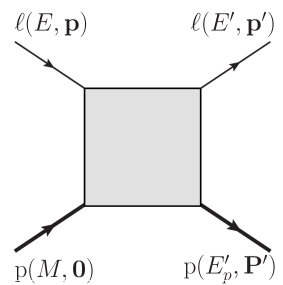
Figure 1: The kinematics of $\ell$p $\to\ell$p scattering in the laboratory frame. The square-shaded area represents all possible internal graphs contributing to the elastic scattering process.

II.1 Leading order TPE contribution

Figure. 2 displays the so-called “box” (planar) and “crossed-box” (non-planar) TPE diagrams, (a) and (b), respectively, contributing at the chiral leading order (LO) amplitude in HB$\chi$PT, and can be expressed in the following 4-point function (namely, with four internal propagators) loop-integral representations:

$${\mathcal{M}^{(a)}_{\rm box}}\!\! = \!\!e^{4}\int\frac{{\rm d}^{4}k}{(2\pi)^{4}i}\frac{\left[\bar{u}(p^{\prime})\gamma^{\mu}(\not{p}-\not{k}+m_{l})\gamma^{\nu}u(p)\right]\left[\chi^{\dagger}(p^{\prime}_{p})v_{\mu}v_{\nu}\chi(p_{p})\right]}{(k^{2}+i0)\,[(Q-k)^{2}+i0]\,(k^{2}-2k\cdot p+i0)\,(v\cdot k+v\cdot p_{p}+i0)}\,,$$ (10)

$${\mathcal{M}^{(b)}_{\rm xbox}}\!\! = \!\!e^{4}\int\frac{{\rm d}^{4}k}{(2\pi)^{4}i}\frac{\left[\bar{u}(p^{\prime})\gamma^{\mu}(\not{p}-\not{k}+m_{l})\gamma^{\nu}u(p)\right]\left[\chi^{\dagger}(p^{\prime}_{p})v_{\mu}v_{\nu}\chi(p_{p})\right]}{(k^{2}+i0)\,[(Q-k)^{2}+i0]\,(k^{2}-2k\cdot p+i0)\,(-v\cdot k+v\cdot p^{\prime}_{p}+i0)}\,,$$ (11)

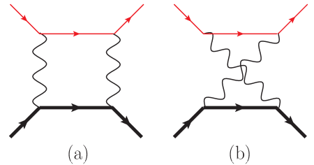
Figure 2: The LO TPE box (a), and crossed-box (b) amplitudes of $\mathcal{O}(\alpha^{2})$, consisting of interactions from the $\mathcal{L}^{(0)}_{\pi N}$ chiral Lagrangian, and contributing to the leading radiative corrections to the unpolarized lepton-proton elastic differential cross-section of $\mathcal{O}(\alpha^{3})$. The thick, thin, and wiggly lines denote the proton, lepton, and photon propagators.

where $u(p)$ and $\bar{u}(p^{\prime})$ are Dirac spinors for incoming and outgoing lepton, while $\chi(p_{p})$ and $\chi(p^{\prime}_{p})$ represent the non-relativistic two-component Pauli spinors for the proton. It must be mentioned that the above two LO TPE diagrams are not strictly LO in the sense that they also contain ${\mathcal{O}}(1/M)$ kinematical recoil terms proportional to $v\cdot Q$ or $v\cdot p^{\prime}_{p}$ which generate contributions commensurate with the dynamical recoil contributions arising from the “NLO TPE” diagrams (c)-(i) (cf. Fig. 3). Likewise, the NLO diagrams generate kinematically suppressed term of ${\mathcal{O}}(1/M^{2})$ commensurate with the dynamical contributions from NNLO TPE diagrams (j)-(v) (cf. Fig. 4). Hence, care must be taken to correctly distinguish between the kinematically and dynamically suppressed subleading terms, all of which scale as ${\mathcal{O}}(1/M^{n})$. Thus, to extract the true bona fide LO TPE cross-section, the resulting ${\mathcal{O}}(1/M)$ terms from diagrams (a) and (b) must be relegated to the NLO part of the TPE amplitudes Talukdar:2019dko ; Choudhary:2023rsz . Particularly, in Ref. Talukdar:2019dko , for a simplistic evaluation of the intricate four-point loop-integration, the authors took recourse to an expansion of the proton propagator in $\mathcal{M}^{(b)}_{\rm xbox}$ in powers of $1/M$ due to the presence of the $v\cdot p^{\prime}_{p}$ term in the denominator and subsequently relocating the ${\mathcal{O}}(1/M)$ terms in the integrand to the NLO level by adding them together with the genuine NLO TPE diagram (h) in Fig. 3. This methodology can certainly be justified for regular integrals leading to finite results. However, in the purview of existing IR-divergences, this simplification potentially undermines the accuracy of the results, as emphasized in the recent work on the exact TPE evaluations in HB$\chi$PT, Ref. Choudhary:2023rsz . Thus, in this work, we do not expand the proton propagators before evaluating the loop-integrals, and instead, follow the approach adopted in Ref. Choudhary:2023rsz . First, we remove the negative sign in front of $v\cdot k$ by a shift of the integration variable $k\rightarrow-k+Q$ in $\mathcal{M}^{(b)}_{\rm xbox}$ leading to

$${\mathcal{M}^{(b)}_{\rm xbox}}=e^{4}\int\frac{{\rm d}^{4}k}{(2\pi)^{4}i}\frac{\left[\bar{u}(p^{\prime})\gamma^{\mu}(\not{p}+\not{k}-\not{Q}+m_{l})\gamma^{\nu}u(p)\right]\left[\chi^{\dagger}(p^{\prime}_{p})v_{\mu}v_{\nu}\chi(p_{p})\right]}{(k^{2}+i0)\,[(Q-k)^{2}+i0]\,(k^{2}+2k\cdot p^{\prime}+i0)\,(v\cdot k+v\cdot p_{p}+i0)}\,.$$ (12)

Next, by invoking SPA (implied henceforth by the symbol $\stackrel{{\scriptstyle\gamma_{\rm soft}}}{{\leadsto}}$), i.e., letting one of the exchange photons as soft (either $k=0$ or $k=Q$) in each of the two LO amplitudes Talukdar:2019dko , we obtain the following two 3-point amplitudes:

$${\mathcal{M}^{(a)}_{\rm box}} \stackrel{{\scriptstyle\gamma_{\rm soft}}}{{\leadsto}} -\,2e^{2}(v\cdot p)\mathcal{M}_{\gamma}^{(0)}\int\frac{{\rm d}^{4}k}{(2\pi)^{4}i}\frac{1}{(k^{2}+i0)\,(k^{2}-2k\cdot p+i0)\,(v\cdot k+i0)}$$

$$-\,2e^{2}(v\cdot p^{\prime})\mathcal{M}_{\gamma}^{(0)}\int\frac{{\rm d}^{4}k}{(2\pi)^{4}i}\frac{1}{[(Q-k)^{2}+i0]\,(k^{2}-2k\cdot p+i0)\,(v\cdot k+i0)}\,,\quad\text{and}$$

$${\mathcal{M}^{(b)}_{\rm xbox}} \stackrel{{\scriptstyle\gamma_{\rm soft}}}{{\leadsto}} -\,2e^{2}(v\cdot p)\mathcal{M}_{\gamma}^{(0)}\int\frac{{\rm d}^{4}k}{(2\pi)^{4}i}\frac{1}{[(Q-k)^{2}+i0]\,(k^{2}+2k\cdot p^{\prime}+i0)\,(v\cdot k+i0)}$$ (13)

$$-\,2e^{2}(v\cdot p^{\prime})\mathcal{M}_{\gamma}^{(0)}\int\frac{{\rm d}^{4}k}{(2\pi)^{4}i}\frac{1}{(k^{2}+i0)\,(k^{2}+2k\cdot p^{\prime}+i0)\,(v\cdot k+i0)}\,.$$

Here, we used the fact that $v\cdot p_{p}=0$ (lab-frame). The resulting sum of the TPE amplitudes in the soft-photon approximation gets factorized into the LO Born amplitude $\mathcal{M}_{\gamma}^{(0)}$ times a $Q^{2}$-dependent function $f^{(ab)}_{\gamma\gamma}(Q^{2})$, namely,

$$\mathcal{M}_{\gamma\gamma}^{(ab)}\!\! = \!\!\mathcal{M}^{(a)}_{\rm box}+\mathcal{M}^{(b)}_{\rm xbox}\stackrel{{\scriptstyle\gamma_{\rm soft}}}{{\leadsto}}\mathcal{M}_{\gamma}^{(0)}f^{(ab)}_{\gamma\gamma}(Q^{2})\,,$$ (14)

where

$${\mathcal{M}}^{(0)}_{\gamma}\!\! = \!\!-\,\frac{e^{2}}{Q^{2}}\big{[}\bar{u}(p^{\prime})\gamma^{\mu}u(p)\big{]}\left[\chi^{\dagger}(p^{\prime}_{p})v_{\mu}\chi(p_{p})\right]\,,\quad\text{and}$$

$$f^{(ab)}_{\gamma\gamma}(Q^{2})\!\! = \!\!-\,2e^{2}\Big{\{}EI^{-}(p,0|1,0,1,1)+E^{\prime}I^{-}(p,0|0,1,1,1)$$

$$\!\!\!+\,EI^{+}(p^{\prime},0|0,1,1,1)+E^{\prime}I^{+}(p^{\prime},0|1,0,1,1)\Big{\}}\,.$$

The relevant real parts of the 3-point loop-integrations $I^{\pm}$ contributing to the elastic cross-section were worked out in Ref. Choudhary:2023rsz up to ${\mathcal{O}}(1/M)$ accuracy. However, in this work, they are needed at the level of ${\mathcal{O}}(1/M^{2})$ whose explicit expressions are provided in the appendix. It is notable that the functions $I^{-}(p,0|1,0,1,1)$ and $I^{+}(p^{\prime},0|1,0,1,1)$ are IR-divergent, while $I^{-}(p,0|0,1,1,1)$ and $I^{+}(p^{\prime},0|0,1,1,1)$ are finite. Moreover, it was shown in Ref. Choudhary:2023rsz that the bona fide LO part [i.e., ${\mathcal{O}}(M^{0})$] of such $I^{\pm}$ integrals are equal but of opposite signs, namely,

$$I^{-}(p,0|1,0,1,1)\!\! \equiv \!\!I^{(0)}(p,0|1,0,1,1)\,,$$

$$I^{+}(p^{\prime},0|1,0,1,1)\!\! = \!\!-\,I^{(0)}(p,0|1,0,1,1)+{\mathcal{O}}\left(M^{-1}\right)\,,$$

$$I^{-}(p,0|0,1,1,1)\!\! = \!\!I^{(0)}(p,0|0,1,1,1)+{\mathcal{O}}\left(M^{-1}\right)\,,$$

$$I^{+}(p^{\prime},0|0,1,1,1)\!\! = \!\!-\,I^{(0)}(p,0|0,1,1,1)+{\mathcal{O}}\left(M^{-1}\right)\,,\qquad\,$$ (16)

where the expressions for $I^{(0)}(p,0|1,0,1,1)$ and $I^{(0)}(p,0|0,1,1,1)$ are also provided in the appendix. Consequently, given that at the true LO in HB$\chi$PT, the incoming and outgoing lepton energies and velocities are the same, i.e., $E=E^{\prime}$ and $\beta=\beta^{\prime}$, respectively, (with $\beta=|{\bf p}|/E$ and $\beta^{\prime}=|{\bf p^{\prime}}|/E^{\prime}$), we find that at the true LO $f^{(0)}_{\gamma\gamma}$ completely vanishes in SPA, i.e., $f^{(0)}_{\gamma\gamma}(Q^{2})\equiv\left[f^{(ab)}_{\gamma\gamma}(Q^{2})\right]_{\rm LO}\!\!\!\!=0$ as in Ref. Talukdar:2019dko . In other words, the ${\mathcal{O}}\left(M^{0}\right)$ IR-divergent terms arising from the genuine LO TPE diagrams (a) and (b) cancel exactly. However, the residual divergences of ${\mathcal{O}}(1/M)$ surviving must be considered commensurate with the subleading chiral order dynamical contributions from NLO or higher-order TPE amplitudes. The fractional TPE corrections to the ${\mathcal{O}}{(\alpha^{2})}$ Born differential cross-section from the LO diagrams (a) and (b) are collected in the ${\mathcal{O}}{(\alpha)}$ term

$$\delta^{(ab)}_{\gamma\gamma}(Q^{2})=\frac{2{\mathcal{R}}e\!\!\!\!\sum\limits_{spins}\!\left[\mathcal{M}_{\gamma}^{(0)*}\mathcal{M}_{\gamma\gamma}^{(ab)}\right]}{\sum\limits_{spins}\left|\mathcal{M}_{\gamma}^{(0)}\right|^{2}}\stackrel{{\scriptstyle\gamma_{\rm soft}}}{{\leadsto}}2{\mathcal{R}}ef^{(ab)}_{\gamma\gamma}(Q^{2}),$$

(17)

where the true LO contributions to the elastic cross-section exactly vanish, namely, $\delta^{(ab);(0)}_{\gamma\gamma}=0$. This is solely an artifact of the SPA approach which potentially spoils the HB$\chi$PT power counting. We know from the recent work of Choudhary et al. Choudhary:2023rsz that an exact analytical evaluation of the true LO diagrams in HB$\chi$PT leads to a non-zero ${\mathcal{O}}\left(M^{0}\right)$ result, namely,

$$\delta^{\rm(0)}_{\gamma\gamma}(Q^{2})=\pi\alpha\frac{\sqrt{-Q^{2}}}{2E}\left(\frac{1}{1+\frac{Q^{2}}{4E^{2}}}\right)\,.$$ (18)

The result is analogous to the well-known McKinley-Feshbach contribution obtained using distorted Born-wave approximation to the second-order in non-relativistic perturbation theory McKinley:1948zz . Thus, to restore the correct power counting we include the above exact result, Eq. (18), as a part of the LO TPE contributions. Using the results of evaluating the 3-point functions $I^{\pm}$ to ${\mathcal{O}}(1/M^{2})$, where the IR-divergent loop-integrals are tackled by employing DR to isolate the IR singularities, we obtain the IR-finite fractional TPE contribution to the differential cross-section in the lab-frame:

$$\overline{\delta^{(ab)}_{\gamma\gamma}}(Q^{2})\!\! = \!\!\delta^{(ab)}_{\gamma\gamma}(Q^{2})-\delta^{\rm(box)}_{\rm IR}(Q^{2})\stackrel{{\scriptstyle\gamma^{*}_{\rm soft}}}{{\leadsto}}\pi\alpha\frac{\sqrt{-Q^{2}}}{2E}\left(\frac{1}{1+\frac{Q^{2}}{4E^{2}}}\right)-\frac{2\alpha Q^{2}}{\pi ME\beta^{2}}\Bigg{[}1-\frac{\pi^{2}}{24}\left(\beta-\frac{1}{\beta}\right)-\ln\sqrt{\frac{2\beta}{1-\beta}}$$ (19)

$$\!\!+\,\frac{1}{2}\left(1-\frac{1}{\beta}\right)\ln\sqrt{\frac{1+\beta}{1-\beta}}+\frac{1}{4}\left(\beta-\frac{1}{\beta}\right)\ln^{2}\sqrt{\frac{1+\beta}{1-\beta}}+\frac{1}{4}\left(\beta-\frac{1}{\beta}\right){\rm Li}_{2}\bigg{(}\frac{1+\beta}{1-\beta}\bigg{)}-\ln\sqrt{-\frac{Q^{2}}{2ME\beta}}$$

$$\!\!\times\,\left\{1+\left(\beta-\frac{1}{\beta}\right)\ln\sqrt{\frac{1+\beta}{1-\beta}}\,\right\}\Bigg{]}-\frac{\alpha Q^{4}}{16\pi M^{2}E^{2}\beta^{5}}\Bigg{[}-\pi^{2}(1-\beta^{2})+8\beta^{3}-8\beta(3+2\beta^{2})\ln{\sqrt{\frac{2\beta}{1-\beta}}}$$

$$\!\!+6(1-\beta^{2})\,{\rm Li}_{2}\!\!\left(\frac{1+\beta}{1-\beta}\right)+6\left(1-\beta^{2}\right)\ln^{2}\sqrt{\frac{1+\beta}{1-\beta}}+4(7+3\beta+2\beta^{3})\ln{\sqrt{\frac{1+\beta}{1-\beta}}}-4\ln\sqrt{-\frac{Q^{2}}{2ME\beta}}$$

$$\!\!\times\,\Bigg{\{}2\beta(3+2\beta^{2})+6(1-\beta^{2})\ln{\sqrt{\frac{1+\beta}{1-\beta}}}\,\Bigg{\}}\,\Bigg{]}+\mathcal{O}\left(\frac{1}{M^{3}}\right)\,.$$

The $\rm{Li}_{2}$ in the equation denotes the standard di-logarithm or Spence function [cf. Eq. (107)]. In SPA the residual IR-divergence from Lo diagrams (a) and (b) are of $\mathcal{O}(1/M)$ and given by

$$\delta^{\rm(box)}_{\rm IR}(Q^{2})\!\! = \!\!\frac{\alpha}{\pi\beta}\left[\frac{1}{\epsilon}-\gamma_{E}+\ln\bigg{(}\frac{4\pi\mu^{2}}{m_{l}^{2}}\bigg{)}\right]\left\{\ln\sqrt{\frac{1+\beta}{1-\beta}}-\frac{\beta}{\beta^{\prime}}\ln\sqrt{\frac{1+\beta^{\prime}}{1-\beta^{\prime}}}\,\right\}$$ (20)

$$= \!\!-\,\frac{\alpha Q^{2}}{2\pi ME\beta^{2}}\left[\frac{1}{\epsilon}-\gamma_{E}+\ln\bigg{(}\frac{4\pi\mu^{2}}{m_{l}^{2}}\bigg{)}\right]\left\{1+\bigg{(}\beta-\frac{1}{\beta}\bigg{)}\ln\sqrt{\frac{1+\beta}{1-\beta}}\,\right\}+$$

$$\!\!+\,\frac{3\alpha Q^{4}}{8\pi M^{2}E^{2}\beta^{4}}\left[\frac{1}{\epsilon}-\gamma_{E}+\ln\bigg{(}\frac{4\pi\mu^{2}}{m_{l}^{2}}\bigg{)}\right]\left\{1-\frac{2}{3}\beta^{2}+\bigg{(}\beta-\frac{1}{\beta}\bigg{)}\ln\sqrt{\frac{1+\beta}{1-\beta}}\,\right\}+\mathcal{O}\left(\frac{1}{M^{3}}\right)\,,$$

where $\epsilon=(4-D)/2<0$. Notably, the above-mentioned singular term $\delta^{\rm(box)}_{\rm IR}(Q^{2})$ is identical to the one obtained in the exact TPE evaluation of Choudhary et al. Choudhary:2023rsz . It will ultimately cancel the IR-divergent counterparts from charge-odd soft-photon ($\gamma^{*}_{\rm soft}$) bremsstrahlung process $\delta^{\rm(soft)}_{\rm IR}$, viz., those singular terms originating from the interference process between the LO lepton-bremsstrahlung and LO proton-bremsstrahlung diagrams contributing to the elastic cross-section, such that, $\delta^{\rm(soft)}_{\rm IR}+\delta^{\rm(box)}_{\rm IR}=0$ Bhoomika24 . Furthermore, it is notable that the singularities from diagrams (a) and (b) are the only sources of IR-divergence in the TPE contributions. No IR-divergent contribution is generated from the subleading-order TPE diagrams. As already mentioned in the introduction, unlike Refs. Talukdar:2019dko ; Talukdar:2020aui , we keep the scheme-dependent IR-divergent terms to be subtracted precisely as given in Eq. (20), without re-adjustments with the finite TPE part unlike in Refs. Talukdar:2019dko ; Talukdar:2020aui .

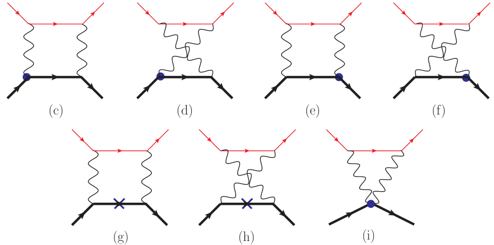
Figure 3: The NLO TPE diagrams of $\mathcal{O}(\alpha^{2}/M)$ contributing to the $\mathcal{O}(\alpha^{3}/M)$ elastic differential cross-section. The thick, thin, and wiggly lines denote the proton, lepton, and photon propagators. The blobs and crosses denote the insertions of the NLO proton-photon vertices and ${\mathcal{O}}(1/M)$ proton propagators, respectively.

II.2 Next-to-leading order TPE contribution

We now turn to the evaluation of the seven NLO TPE diagrams (c)-(i), displayed in Fig. 3. Each amplitude either consists of one insertion of proton-photon interaction vertex arising from the NLO Lagrangian ${\mathcal{L}}^{(1)}_{\pi N}$ or from the NLO proton propagator [i.e., the $\mathcal{O}(1/M)$ term in Eq. (II)]. The TPE amplitudes are given by the following integral representations Choudhary:2023rsz :

$${\mathcal{M}^{(c)}_{\rm box}}\!\! = \!\!\frac{e^{4}}{2M}\int\frac{{\rm d}^{4}k}{(2\pi)^{4}i}\frac{\left[\bar{u}(p^{\prime})\gamma^{\mu}(\not{p}-\not{k}+m_{l})\gamma^{\nu}u(p)\right]\,\left[\chi^{\dagger}(p_{p}^{\prime})\Big{\{}v_{\mu}(k+2p_{p})_{\nu}-v_{\mu}v_{\nu}[v\cdot(k+2p_{p})]\Big{\}}\chi(p_{p})\right]}{(k^{2}+i0)\,[(Q-k)^{2}+i0]\,(k^{2}-2k\cdot p+i0)\,(v\cdot k+v\cdot p_{p}+i0)}\,,\qquad\,$$ (21)

$${\mathcal{M}^{(d)}_{\rm xbox}}\!\! = \!\!\frac{e^{4}}{2M}\int\frac{{\rm d}^{4}k}{(2\pi)^{4}i}\frac{\left[\bar{u}(p^{\prime})\gamma^{\mu}(\not{p}-\not{k}+m_{l})\gamma^{\nu}u(p)\right]\,\left[\chi^{\dagger}(p_{p}^{\prime})\Big{\{}v_{\nu}(p_{p}+p^{\prime}_{p}-k)_{\mu}-v_{\mu}v_{\nu}[v\cdot(p_{p}+p_{p}^{\prime}-k)]\Big{\}}\chi(p_{p})\right]}{(k^{2}+i0)\,[(Q-k)^{2}+i0]\,(k^{2}-2k\cdot p+i0)\,(-v\cdot k+v\cdot p_{p}^{\prime}+i0)}\,,\qquad\,$$ (22)

$${\mathcal{M}^{(e)}_{\rm box}}\!\! = \!\!\frac{e^{4}}{2M}\int\frac{{\rm d}^{4}k}{(2\pi)^{4}i}\frac{\left[\bar{u}(p^{\prime})\gamma^{\mu}(\not{p}-\not{k}+m_{l})\gamma^{\nu}u(p)\right]\,\left[\chi^{\dagger}(p^{\prime}_{p})\Big{\{}v_{\nu}(p_{p}+p^{\prime}_{p}+k)_{\mu}-v_{\mu}v_{\nu}[v\cdot(p_{p}+p^{\prime}_{p}+k)]\Big{\}}\chi(p_{p})\right]}{(k^{2}+i0)\,[(Q-k)^{2}+i0]\,(k^{2}-2k\cdot p+i0)\,(v\cdot k+v\cdot p_{p}+i0)}\,,\qquad\,$$ (23)

$${\mathcal{M}^{(f)}_{\rm xbox}}\!\! = \!\!\frac{e^{4}}{2M}\int\frac{{\rm d}^{4}k}{(2\pi)^{4}i}\frac{\left[\bar{u}(p^{\prime})\gamma^{\mu}(\not{p}-\not{k}+m_{l})\gamma^{\nu}u(p)\right]\,\left[\chi^{\dagger}(p^{\prime}_{p})\Big{\{}v_{\mu}(2p^{\prime}_{p}-k)_{\nu}-v_{\mu}v_{\nu}[v\cdot(2p^{\prime}_{p}-k)]\Big{\}}\chi(p_{p})\right]}{(k^{2}+i0)\,[(Q-k)^{2}+i0]\,(k^{2}-2k\cdot p+i0)\,(-v\cdot k+v\cdot p^{\prime}_{p}+i0)}\,,\qquad\,$$ (24)

$${\mathcal{M}^{(g)}_{\rm box}}\!\! = \!\!\frac{e^{4}}{2M}\int\frac{{\rm d}^{4}k}{(2\pi)^{4}i}\frac{\left[\bar{u}(p^{\prime})\gamma^{\mu}(\not{p}-\not{k}+m_{l})\gamma^{\nu}u(p)\right]\,\left[\chi^{\dagger}(p^{\prime}_{p})v_{\mu}v_{\nu}\chi(p_{p})\right]}{(k^{2}+i0)\,[(Q-k)^{2}+i0]\,(k^{2}-2k\cdot p+i0)}\left(1-\frac{(p_{p}+k)^{2}}{(v\cdot p_{p}+v\cdot k+i0)^{2}}\right)\,,\qquad\,$$ (25)

$${\mathcal{M}^{(h)}_{\rm xbox}}\!\! = \!\!\frac{e^{4}}{2M}\int\frac{{\rm d}^{4}k}{(2\pi)^{4}i}\frac{\left[\bar{u}(p^{\prime})\gamma^{\mu}(\not{p}-\not{k}+m_{l})\gamma^{\nu}u(p)\right]\,\left[\chi^{\dagger}(p^{\prime}_{p})v_{\mu}v_{\nu}\chi(p_{p})\right]}{(k^{2}+i0)\,[(Q-k)^{2}+i0]\,(k^{2}-2k\cdot p+i0)}\left(1-\frac{(p^{\prime}_{p}-k)^{2}}{(v\cdot p^{\prime}_{p}-v\cdot k+i0)^{2}}\right)\,,\qquad\,$$ (26)

$${\mathcal{M}^{(i)}_{\rm seagull}}\!\! = \!\!\frac{e^{4}}{M}\int\frac{{\rm d}^{4}k}{(2\pi)^{4}i}\frac{\left[\bar{u}(p^{\prime})\gamma^{\mu}(\not{p}-\not{k}+m_{l})\gamma^{\nu}u(p)\right]\,\left[\chi^{\dagger}(p^{\prime}_{p})(v_{\mu}v_{\nu}-g_{\mu\nu})\chi(p_{p})\right]}{(k^{2}+i0)\,[(Q-k)^{2}+i0]\,(k^{2}-2k\cdot p+i0)}\,.\qquad\,$$ (27)

The following comments are in order:

• As in Ref. Talukdar:2019dko , some of the $v_{\mu}v_{\nu}$ terms cancel between $\mathcal{M}^{(c)}_{\rm box}$, $\mathcal{M}^{(f)}_{\rm box}$, $\mathcal{M}^{(g)}_{\rm box}$, $\mathcal{M}^{(h)}_{\rm xbox}$ and $\mathcal{M}^{(i)}_{\rm seagull}$.

• The expressions for $\mathcal{M}^{(h)}_{\rm xbox}$ is written differently from that of Ref. Talukdar:2019dko , as they do not include the ${\mathcal{O}}(1/M)$ kinematically suppressed terms arising from the expansion of the LO TPE diagram (b). In Ref. Talukdar:2019dko they were omitted in the LO contributions by relocating them alongside the NLO TPE diagram (h).

• Unlike Ref. Talukdar:2019dko , we here preserve the kinetic energy terms such as $v\cdot p_{p}$ and $v\cdot p^{\prime}_{p}$ in the propagator denominators. Hence, $\mathcal{M}^{(g)}_{\rm box}$ and $\mathcal{M}^{(h)}_{\rm xbox}$ do not mutually yield a vanishing contribution.

• Since $v\cdot p^{\prime}_{p}=v\cdot Q\sim\mathcal{O}(1/M)$, in the NLO analysis of Ref. Talukdar:2019dko such terms were neglected in the numerators of the NLO TPE diagrams since they yielded $\mathcal{O}(1/M^{2})$ terms which are beyond the intended accuracy. However, in this TPE analysis, since we intend to include the proton’s structure effects at NNLO which yield $\mathcal{O}(1/M^{2})$ terms, it is important to retain all $\mathcal{O}(1/M^{2})$ kinematically suppressed terms arising from the NLO, as well as the LO TPE analysis.

After shifting the integration variable $k\rightarrow-k+Q$ in the NLO crossed-box diagrams and including the partial cancellation between $v_{\mu}v_{\nu}$ terms, with $v\cdot p_{p}=0$, yield the following reduced NLO amplitudes:

$${\widetilde{\mathcal{M}}^{(c)}_{\rm box}}\!\! = \!\!\frac{e^{4}}{2M}\int\frac{{\rm d}^{4}k}{(2\pi)^{4}i}\frac{[\bar{u}(p^{\prime})\gamma^{\mu}(\not{p}-\not{k}+m_{l})\gamma^{\nu}u(p)]\Big{[}\chi^{\dagger}(p^{\prime}_{p})v_{\mu}k_{\nu}\chi(p_{p})\Big{]}}{(k^{2}+i0)\,[(Q-k)^{2}+i0]\,(k^{2}-2k\cdot p+i0)\,(v\cdot k+i0)}\,,$$ (28)

$${\widetilde{\mathcal{M}}^{(d)}_{\rm xbox}}\!\! = \!\!\frac{e^{4}}{2M}\int\frac{{\rm d}^{4}k}{(2\pi)^{4}i}\frac{[\bar{u}(p^{\prime})\gamma^{\mu}(\not{p}+\not{k}-\not{Q}+m_{l})\gamma^{\nu}u(p)]\Big{[}\chi^{\dagger}(p^{\prime}_{p})v_{\nu}k_{\mu}\chi(p_{p})\Big{]}}{(k^{2}+i0)\,[(Q-k)^{2}+i0]\,(k^{2}+2k\cdot p^{\prime}+i0)\,(v\cdot k+i0)},$$ (29)

$${\widetilde{\mathcal{M}}^{(e)}_{\rm box}}\!\! = \!\!\frac{e^{4}}{2M}\int\frac{{\rm d}^{4}k}{(2\pi)^{4}i}\frac{[\bar{u}(p^{\prime})\gamma^{\mu}(\not{p}-\not{k}+m_{l})\gamma^{\nu}u(p)]\Big{[}\chi^{\dagger}(p^{\prime}_{p})v_{\nu}(Q+k)_{\mu}\chi(p_{p})\Big{]}}{(k^{2}+i0)\,[(Q-k)^{2}+i0]\,(k^{2}-2k\cdot p+i0)\,(v\cdot k+i0)}\,,$$ (30)

$${\widetilde{\mathcal{M}}^{(f)}_{\rm xbox}}\!\! = \!\!\frac{e^{4}}{2M}\int\frac{{\rm d}^{4}k}{(2\pi)^{4}i}\frac{[\bar{u}(p^{\prime})\gamma^{\mu}(\not{p}+\not{k}-\not{Q}+m_{l})\gamma^{\nu}u(p)]\Big{[}\chi^{\dagger}(p^{\prime}_{p})v_{\mu}(k+Q)_{\nu}\chi(p_{p})\Big{]}}{(k^{2}+i0)\,[(Q-k)^{2}+i0]\,(k^{2}+2k\cdot p^{\prime}+i0)\,(v\cdot k+i0)}\,,$$ (31)

$${\widetilde{\mathcal{M}}^{(g)}_{\rm box}}\!\! = \!\!\frac{e^{4}}{2M}\int\frac{{\rm d}^{4}k}{(2\pi)^{4}i}\frac{[\bar{u}(p^{\prime})\gamma^{\mu}(\not{p}-\not{k}+m_{l})\gamma^{\nu}u(p)]\Big{[}\chi^{\dagger}(p^{\prime}_{p})v_{\mu}v_{\nu}\chi(p_{p})\Big{]}}{(k^{2}+i0)\,[(Q-k)^{2}+i0]\,(k^{2}-2k\cdot p+i0)}\left(-\frac{k^{2}}{(v\cdot k+i0)^{2}}\right)\,,$$ (32)

$${\widetilde{\mathcal{M}}^{(h)}_{\rm xbox}}\!\! = \!\!\frac{e^{4}}{2M}\int\frac{{\rm d}^{4}k}{(2\pi)^{4}i}\frac{[\bar{u}(p^{\prime})\gamma^{\mu}(\not{p}+\not{k}-\not{Q}+m_{l})\gamma^{\nu}u(p)]\Big{[}\chi^{\dagger}(p^{\prime}_{p})v_{\mu}v_{\nu}\chi(p_{p})\Big{]}}{(k^{2}+i0)\,[(Q-k)^{2}+i0]\,(k^{2}+2k\cdot p^{\prime}+i0)}\left(-\frac{k^{2}}{(v\cdot k+i0)^{2}}\right)\,,$$ (33)

$${\widetilde{\mathcal{M}}^{(i)}_{\rm seagull}}\!\! = \!\!-\,\frac{e^{4}}{M}\int\frac{{\rm d}^{4}k}{(2\pi)^{4}i}\frac{[\bar{u}(p^{\prime})\gamma^{\mu}(\not{p}-\not{k}+m_{l})\gamma_{\mu}u(p)]\Big{[}\chi^{\dagger}(p^{\prime}_{p})\chi(p_{p})\Big{]}}{(k^{2}+i0)\,[(Q-k)^{2}+i0]\,(k^{2}-2k\cdot p+i0)}\,.$$ (34)

The residual part of the seagull amplitude ${\widetilde{\mathcal{M}}^{(i)}_{\rm seagull}}$ is already a 3-point integral, and thus, evaluated exactly. In fact, using SPA for the 3-point amplitudes like the seagull diagram leads to unphysical UV divergence, which should be absent for all one-loop TPE diagrams, without the inclusion of additional pion-loops. Hence, for the NLO diagrams, SPA is limited to the evaluation of the box and crossed amplitudes (c)-(h) to reduce the complicated 4-point functions into 3-point functions. As seen in the ensuing analysis, all contributions are IR/UV finite at NLO. Thus, after invoking SPA we find that the amplitudes either factorize into the LO Born amplitude $\mathcal{M}_{\gamma}^{(0)}$, Eq. (LABEL:eq:M0_LO), or into the amplitude

$${\mathcal{N}}^{(1)}_{\gamma}=-\frac{e^{2}}{MQ^{2}}\big{[}\bar{u}(p^{\prime})\gamma^{\mu}u(p)\big{]}\left[\chi^{\dagger}(p^{\prime}_{p})Q_{\mu}\chi(p_{p})\right]\,,$$ (35)

which form a part of the NLO correction to the LO Born amplitude ${\mathcal{M}}^{(1)}_{\gamma}$ for elastic lepton-proton scattering in HB$\chi$PT expressed in the lab-frame, i.e., with $p^{\prime}_{p}=Q$:

$${\mathcal{M}}^{(1)}_{\gamma}=\frac{1}{2}{\mathcal{N}}^{(1)}_{\gamma}+\frac{e^{2}}{2MQ^{2}}\big{[}\bar{u}(p^{\prime})\gamma^{\mu}u(p)\big{]}\Big{[}\chi^{\dagger}(p^{\prime}_{p})\Big{\{}v_{\mu}(v\cdot Q)-(2+\kappa_{s}+\kappa_{v})[S_{\mu},S\cdot Q]\Big{\}}\chi(p_{p})\Big{]}\,.$$ (36)

Thus, the NLO box and crossed-box TPE amplitudes reduce in SPA from the original 4-point to the 3-point functions:

$${\widetilde{\mathcal{M}}^{(c)}_{\rm box}} \stackrel{{\scriptstyle\gamma_{\rm soft}}}{{\leadsto}} -\,e^{2}E^{\prime}{\mathcal{N}}^{(1)}_{\gamma}\int\frac{{\rm d}^{4}k}{(2\pi)^{4}i}\frac{1}{[(Q-k)^{2}+i0](k^{2}-2k\cdot p+i0)(v\cdot k+i0)}\,,$$ (37)

$${\widetilde{\mathcal{M}}^{(d)}_{\rm xbox}} \stackrel{{\scriptstyle\gamma_{\rm soft}}}{{\leadsto}} -\,e^{2}E{\mathcal{N}}^{(1)}_{\gamma}\int\frac{{\rm d}^{4}k}{(2\pi)^{4}i}\frac{1}{[(Q-k)^{2}+i0]\,(k^{2}+2k\cdot p^{\prime}+i0)\,(v\cdot k+i0)}\,,$$ (38)

$${\widetilde{\mathcal{M}}^{(e)}_{\rm box}} \stackrel{{\scriptstyle\gamma_{\rm soft}}}{{\leadsto}} -\,e^{2}E{\mathcal{N}}^{(1)}_{\gamma}\int\frac{{\rm d}^{4}k}{(2\pi)^{4}i}\frac{1}{(k^{2}+i0)\,(k^{2}-2k\cdot p+i0)\,(v\cdot k+i0)}$$ (39)

$$+\,\frac{e^{2}Q^{2}}{M}\mathcal{M}_{\gamma}^{(0)}\int\frac{{\rm d}^{4}k}{(2\pi)^{4}i}\frac{1}{[(Q-k)^{2}+i0]\,(k^{2}-2k\cdot p+i0)\,(v\cdot k+i0)}\,,$$

$${\widetilde{\mathcal{M}}^{(f)}_{\rm xbox}} \stackrel{{\scriptstyle\gamma_{\rm soft}}}{{\leadsto}} -\,e^{2}E^{\prime}{\mathcal{N}}^{(1)}_{\gamma}\int\frac{{\rm d}^{4}k}{(2\pi)^{4}i}\frac{1}{(k^{2}+i0)\,(k^{2}+2k\cdot p^{\prime}+i0)\,(v\cdot k+i0)}$$ (40)

$$-\,\frac{e^{2}Q^{2}}{M}\mathcal{M}_{\gamma}^{(0)}\int\frac{{\rm d}^{4}k}{(2\pi)^{4}i}\frac{1}{[(Q-k)^{2}+i0]\,(k^{2}+2k\cdot p^{\prime}+i0)\,(v\cdot k+i0)}\,,$$

$${\widetilde{\mathcal{M}}^{(g)}_{\rm box}} \stackrel{{\scriptstyle\gamma_{\rm soft}}}{{\leadsto}} \frac{e^{2}E^{\prime}Q^{2}}{M}\mathcal{M}_{\gamma}^{(0)}\int\frac{{\rm d}^{4}k}{(2\pi)^{4}i}\frac{1}{[(Q-k)^{2}+i0]\,(k^{2}-2k\cdot p+i0)\,(v\cdot k+i0)^{2}}\,,$$ (41)

$${\widetilde{\mathcal{M}}^{(h)}_{\rm xbox}} \stackrel{{\scriptstyle\gamma_{\rm soft}}}{{\leadsto}} \frac{e^{2}EQ^{2}}{M}\mathcal{M}_{\gamma}^{(0)}\int\frac{{\rm d}^{4}k}{(2\pi)^{4}i}\frac{1}{[(Q-k)^{2}+i0]\,(k^{2}+2k\cdot p^{\prime}+i0)\,(v\cdot k+i0)^{2}}\,.$$ (42)

Since we go beyond the NLO evaluation of Ref. Talukdar:2019dko by including NNLO corrections, we refrain from substituting $E=E^{\prime}$ and $\beta=\beta^{\prime}$. However, we find it legitimate to use this kind of approximation to evaluate the genuine NNLO diagrams. Unlike Ref. Talukdar:2019dko , the sum of the TPE amplitudes (g) and (h) do not exactly cancel in our case and rather yield residual terms of ${\mathcal{O}}(1/M^{2})$. In other words, $\widetilde{\mathcal{M}}^{(g)}_{\rm box}+\widetilde{\mathcal{M}}^{(h)}_{\rm xbox}\sim{\mathcal{O}}(1/M^{2})$, which is formally commensurate with the dynamical contributions from the NNLO TPE diagrams. Thus, the sum of the NLO amplitudes is summarized as

$$\mathcal{M}^{(cde\cdots i)}_{\gamma\gamma}\!\! = \!\!\widetilde{\mathcal{M}}_{\rm box}^{(c)}+\widetilde{\mathcal{M}}_{\rm xbox}^{(d)}+\widetilde{\mathcal{M}}_{\rm box}^{(e)}+\widetilde{\mathcal{M}}_{\rm xbox}^{(f)}$$ (43)

$$\!\!+\,\widetilde{\mathcal{M}}_{\rm box}^{(g)}+\widetilde{\mathcal{M}}_{\rm xbox}^{(h)}+{\widetilde{\mathcal{M}}^{(i)}_{\rm seagull}}$$

$$\stackrel{{\scriptstyle\gamma_{\rm soft}}}{{\leadsto}} \mathcal{M}_{\gamma}^{(0)}f^{(cde\cdots h)}_{\gamma\gamma}(Q^{2})+{\widetilde{\mathcal{M}}^{(i)}_{\rm seagull}}\,,$$

where

$$f^{(cde\cdots h)}_{\gamma\gamma}(Q^{2})\!\! = \!\!-\,\frac{e^{2}Q^{2}}{M}\bigg{\{}-I^{-}(p,0|0,1,1,1)+I^{+}(p^{\prime},0|0,1,1,1)-E^{\prime}I^{-}(p,0|0,1,1,2)-EI^{+}(p^{\prime},0|0,1,1,2)\bigg{\}}$$

$$\!\!-\,\frac{e^{2}{\mathcal{M}}^{(0)*}_{\gamma}{\mathcal{N}}^{(1)}_{\gamma}}{\left|{\mathcal{M}}^{(0)}_{\gamma}\right|^{2}}\bigg{\{}E^{\prime}I^{-}(p,0|0,1,1,1)+EI^{+}(p^{\prime},0|0,1,1,1)+EI^{-}(p,0|1,0,1,1)+E^{\prime}I^{+}(p,0|1,0,1,1)\bigg{\}}\,.$$

Here we use the same definitions of the loop-integrals $I^{-}(p,0|1,0,1,1)$, $I^{-}(p,0|0,1,1,1)$, $I^{+}(p^{\prime},0|0,1,1,1)$, $I^{+}(p^{\prime},0|1,0,1,1)$, $I^{-}(p,0|0,1,1,2)$ and $I^{+}(p^{\prime},0|0,1,1,2)$, as in Ref. Choudhary:2023rsz . The analytical expressions of these integrals evaluated to ${\mathcal{O}}(1/M^{2})$ are displayed in the appendix. It is notable that even though the above amplitude contains IR-divergent integrals $I^{-}(p,0|1,0,1,1)$ and $I^{+}(p^{\prime},0|1,0,1,1)$, in effect they do not contribute to the cross-section. The reason is that the pre-factor ${\mathcal{M}}^{(0)*}_{\gamma}{\mathcal{N}}^{(1)}_{\gamma}$ causes the entire expression in the second-line of Eq. (II.2) to vanish identically when evaluating the cross-section, namely,

$$\sum\limits_{spins}\left[{\mathcal{M}}^{(0)*}_{\gamma}{\mathcal{N}}^{(1)}_{\gamma}\right]=0\,.$$

The $\mathcal{O}(\alpha/M)$ fractional TPE corrections (relative to the LO) to the elastic differential cross-section from the NLO diagrams are then collected within the term

$$\delta^{(cde\cdots i)}_{\gamma\gamma}(Q^{2})=\frac{2{\mathcal{R}}e\sum\limits_{spins}\left[\mathcal{M}_{\gamma}^{(0)*}{\mathcal{M}}_{\gamma\gamma}^{(cde\cdots i)}\right]}{\sum\limits_{spins}\left|\mathcal{M}_{\gamma}^{(0)}\right|^{2}}=\delta^{(cde\cdots h)}_{\gamma\gamma}(Q^{2})+\delta_{\gamma\gamma;{\rm NLO}}^{\rm(seagull)}(Q^{2})\,,$$ (45)

where the contributions from the TPE box and crossed-box diagrams (c)-(h) are given as

$$\delta^{(cde\cdots h)}_{\gamma\gamma}(Q^{2}) \stackrel{{\scriptstyle\gamma_{\rm soft}}}{{\leadsto}} 2{\mathcal{R}}ef^{(cde\cdots h)}_{\gamma\gamma}(Q^{2})=\frac{\alpha Q^{2}}{\pi ME\beta^{2}}\Bigg{[}1-\frac{\pi^{2}}{6}\beta-\left(\frac{1}{\beta}+\beta\right)\ln\sqrt{\frac{1+\beta}{1-\beta}}+2\beta\ln^{2}\!\!\sqrt{\frac{1+\beta}{1-\beta}}-4\beta\ln\!\sqrt{-\frac{Q^{2}}{2ME\beta}}$$ (46)

$$\!\!\times\,\ln\sqrt{\frac{1+\beta}{1-\beta}}+\beta{\rm Li}_{2}\bigg{(}\frac{2\beta}{1+\beta}\bigg{)}+\beta{\rm Li}_{2}\bigg{(}\frac{1+\beta}{1-\beta}\bigg{)}\Bigg{]}+\frac{\alpha Q^{4}}{24\pi M^{2}E^{2}\beta^{5}}\Bigg{[}\pi^{2}\beta^{2}-54\beta-24\beta^{3}\ln\sqrt{\frac{2\beta}{1-\beta}}$$

$$\!\!-12\beta^{2}\ln^{2}\sqrt{\frac{1+\beta}{1-\beta}}-6\beta^{2}{\rm Li}_{2}\left(\frac{1+\beta}{1-\beta}\right)-6\beta^{2}{\rm Li}_{2}\left(\frac{2\beta}{1+\beta}\right)+6\left(3+3\beta^{2}+2\beta^{3}\right)\ln{\sqrt{\frac{1+\beta}{1-\beta}}}$$

$$\!\!-24\beta^{2}\!\ln\sqrt{-\frac{Q^{2}}{2M\beta E}}\left(\beta-\ln{\sqrt{\frac{1+\beta}{1-\beta}}}\,\right)\Bigg{]}+{\mathcal{O}}\left(\frac{1}{M^{3}}\right)\,,$$

and that of the seagull diagram (i) is given as

$$\delta_{\gamma\gamma;{\rm NLO}}^{\rm(seagull)}(Q^{2})\!\! = \!\!\frac{4\pi\alpha}{M}\bigg{[}\frac{Q^{2}}{Q^{2}+4EE^{\prime}}\bigg{]}\,{\mathcal{R}}e\bigg{\{}4(Q^{2}v+2Ep+2Ep^{\prime})\cdot I^{-}_{1}(p,0|1,1,1,0)+16m_{l}^{2}EI(Q|1,1,1,0)\bigg{\}}$$

$$= \!\!-\,\frac{4\alpha E}{\pi M}\bigg{[}\frac{Q^{2}}{Q^{2}+4E^{2}}\bigg{]}\left(\frac{\nu_{l}^{2}-1}{\nu_{l}^{2}}\right)\Bigg{[}\left(\frac{1+\nu_{l}^{2}}{2\nu_{l}}\right)\bigg{\{}\frac{\pi^{2}}{3}+\ln^{2}{\sqrt{\frac{\nu_{l}+1}{\nu_{l}-1}}+{\rm Li}_{2}\left(\frac{\nu_{l}-1}{\nu_{l}+1}\right)}\bigg{\}}-\ln\sqrt{-\frac{Q^{2}}{m_{l}^{2}}}\,\,\Bigg{]}$$

$$\!\!+\,\frac{8\alpha E^{2}}{\pi M^{2}}\bigg{[}\frac{Q^{2}}{Q^{2}+4E^{2}}\bigg{]}^{2}\left(\frac{\nu_{l}^{2}-1}{\nu_{l}^{2}}\right)\Bigg{[}\left(\frac{1+\nu_{l}^{2}}{2\nu_{l}}\right)\bigg{\{}\frac{\pi^{2}}{3}+\ln^{2}{\sqrt{\frac{\nu_{l}+1}{\nu_{l}-1}}+{\rm Li}_{2}\left(\frac{\nu_{l}-1}{\nu_{l}+1}\right)}\bigg{\}}-\ln\sqrt{-\frac{Q^{2}}{m_{l}^{2}}}\,\,\Bigg{]}$$

$$\!\!-\,\frac{\alpha Q^{2}}{2\pi M^{2}\nu_{l}^{2}}\bigg{[}\frac{Q^{2}}{Q^{2}+4E^{2}}\bigg{]}\Bigg{[}\!\left(\frac{\nu_{l}^{2}-1}{\nu_{l}}\right)\!\bigg{\{}\frac{\pi^{2}}{3}+\ln^{2}{\sqrt{\frac{\nu_{l}+1}{\nu_{l}-1}}+{\rm Li}_{2}\left(\frac{\nu_{l}-1}{\nu_{l}+1}\right)}\bigg{\}}+2\ln\sqrt{-\frac{Q^{2}}{m_{l}^{2}}}\,\Bigg{]}\!+\!\mathcal{O}\left(\!\frac{1}{M^{3}}\!\right).$$

Here, $\nu_{l}=\sqrt{1-4m^{2}_{l}/Q^{2}}$ is a $Q^{2}$-dependent kinematical variable. The definition of the relativistic three-point scalar and tensor loop-integrals, $I(Q|1,1,1,0)$ and $I^{-\mu}_{1}(p,0|1,1,1,0)$, respectively, are taken from Ref. Choudhary:2023rsz . For completeness, their analytical expressions are provided in the appendix. In particular, the expression for the above seagull contribution is slightly more general than what was presented in Ref. Talukdar:2019dko , where the evaluation was carried out only to $\mathcal{O}(1/M)$. Retaining all $\mathcal{O}\left(1/M^{2}\right)$ kinematically suppressed terms arising beyond the NLO contributions are essential, as they must be considered formally at the same footing with the dynamical contributions from the genuine NNLO TPE diagrams which we consider next.

II.3 Next-to-next-to-leading order TPE contribution

Next, we evaluate the thirteen NNLO TPE one-loop diagrams (j)-(v), displayed in Fig 4. The diagrams are constructed based on the following components: (i) two insertions of NLO proton-photon effective vertices, (ii) one NLO proton-photon vertex and an $\mathcal{O}(1/M)$ proton propagator, and (iii) one insertion of either an NNLO proton-photon vertex or $\mathcal{O}(1/M^{2})$ proton propagator. We must emphasize that the effective proton-photon vertices include all possible UV-divergent pion-loops with counterterms relevant to this order that also contribute to the iso-scalar and iso-vector nucleon form factors (see e.g., Refs. Bernard:1995dp ; Bernard:1998gv ). Thus, diagrams (p)-(s) are constituted essentially from two-loop TPE graphs which factorize into a photon- and a pion-loop contributing to the renormalized proton vertices. Besides such “form factor” type TPE graphs, there are other two-loop TPE graphs including complicated non-factorizable photon and pion loops contributing to the NNLO corrections (cf. Fig. 5). In this work, however, we shall restrict our analysis only to the “effective” one-loop accuracy, namely, including only the form factor type contributions from the proton’s structure to TPE. To this end, the effective renormalized NNLO proton-photon vertex in HB$\chi$PT attributed to pion-loops and LECs like the proton’s anomalous magnetic moment $\kappa_{p}=(\kappa_{s}+\kappa_{v})/2=1.795$, is given by Talukdar:2020aui

$$\mathcal{V}_{\mu}^{(2);{\rm ren}}\!\! = \!\!(F_{1}^{p}-1)v_{\mu}+\frac{1}{M}\bigg{\{}(F_{1}^{p}-1)\left(Q_{\mu}+\frac{Q^{2}}{2M}v_{\mu}\right)+2(F_{1}^{p}+F_{2}^{p}-1-\kappa_{p})[S_{\mu},S\cdot Q]\bigg{\}}$$ (48)

$$\!\!-\,\frac{Q^{2}}{8M^{2}}(F_{1}^{p}-2F_{2}^{p}-1)v_{\mu}+{\mathcal{O}}\left(\frac{1}{M^{3}}\right)\,,$$

where the proton’s Dirac and Pauli form factors $F_{1,2}^{p}$, to $\mathcal{O}(1/M^{2})$, can be Taylor expanded at low-energies in terms of the corresponding Dirac and Pauli mean square radii, $\langle r^{2}_{1,2}\rangle\sim\mathcal{O}(1/M^{2})$, and the anomalous magnetic moment, $\kappa_{p}\sim\mathcal{O}(M^{0})$ (see Ref. Bernard:1998gv for details):

$$F_{1}^{p}(Q^{2})\!\! = \!\!1+\frac{Q^{2}}{6}\langle r_{1}^{2}\rangle+\mathcal{O}(M^{-3})\,,\quad\text{and}$$

$$F_{2}^{p}(Q^{2})\!\! = \!\!\kappa_{p}+\frac{Q^{2}}{6}\langle r^{2}_{2}\rangle+\mathcal{O}(M^{-3})\,.$$ (49)

It turns out that for the NNLO TPE and other radiative corrections up to $\mathcal{O}(1/M^{2})$ suppressed terms, only the Dirac radius contributes at this order, which in turn can be related to the proton’s root mean square (rms) electric or charge radius $r_{p}\equiv\sqrt{\langle r^{2}_{E}\rangle}$, namely,

$$\langle r^{2}_{1}\rangle=\langle r^{2}_{E}\rangle-\frac{3\kappa_{p}}{2M^{2}}+\mathcal{O}(M^{-3})\,.$$ (50)

We now spell out the NNLO amplitudes given by the following integral representations:

$${\mathcal{M}^{(j)}_{\rm box}}\!\! = \!\!\frac{e^{4}}{4M^{2}}\int\frac{{\rm d}^{4}k}{(2\pi)^{4}i}\frac{\left[\bar{u}(p^{\prime})\gamma^{\mu}(\not{p}-\not{k}+m_{l})\gamma^{\nu}u(p)\right]}{(k^{2}+i0)\,[(Q-k)^{2}+i0]\,(k^{2}-2k\cdot p+i0)\,(v\cdot p_{p}+v\cdot k+i0)}$$ (51)

$$\hskip 28.45274pt\times\left[\chi^{\dagger}(p^{\prime}_{p})\Big{\{}(p_{p}+p_{p}^{\prime}+k)_{\mu}-v_{\mu}[v\cdot(p_{p}+p_{p}^{\prime}+k)]\Big{\}}\,\Big{\{}(2p_{p}+k)_{\nu}-v_{\nu}[v\cdot(2p_{p}+k)]\Big{\}}\chi(p_{p})\right]\,,$$

$${\mathcal{M}^{(k)}_{\rm xbox}}\!\! = \!\!\frac{e^{4}}{4M^{2}}\int\frac{{\rm d}^{4}k}{(2\pi)^{4}i}\frac{\left[\bar{u}(p^{\prime})\gamma^{\mu}(\not{p}-\not{k}+m_{l})\gamma^{\nu}u(p)\right]}{(k^{2}+i0)\,[(Q-k)^{2}+i0]\,(k^{2}-2k\cdot p+i0)\,(v\cdot p_{p}^{\prime}-v\cdot k+i0)}$$ (52)

$$\hskip 28.45274pt\times\left[\chi^{\dagger}(p^{\prime}_{p})\Big{\{}(2p_{p}^{\prime}-k)_{\nu}-v_{\nu}v\cdot(2p_{p}^{\prime}-k)\Big{\}}\,\Big{\{}(p_{p}^{\prime}+p_{p}-k)_{\mu}-v_{\mu}[v\cdot(p_{p}^{\prime}+p_{p}-k)]\Big{\}}\chi(p_{p})\right]\,,$$

$${\mathcal{M}^{(l)}_{\rm box}}\!\! = \!\!\frac{e^{4}}{4M^{2}}\int\frac{{\rm d}^{4}k}{(2\pi)^{4}i}\frac{\left[\bar{u}(p^{\prime})\gamma^{\mu}(\not{p}-\not{k}+m_{l})\gamma^{\nu}u(p)\right]\left[\chi^{\dagger}(p^{\prime}_{p})\Big{\{}v_{\mu}(2p_{p}+k)_{\nu}-v_{\mu}v_{\nu}[v\cdot(2p_{p}+k)]\Big{\}}\chi(p_{p})\right]}{(k^{2}+i0)\,[(Q-k)^{2}+i0]\,(k^{2}-2k\cdot p+i0)}$$ (53)

$$\hskip 28.45274pt\times\left(1-\frac{(p_{p}+k)^{2}}{(v\cdot p_{p}+v\cdot k+i0)^{2}}\right)\,,$$

$${\mathcal{M}^{(m)}_{\rm xbox}}\!\! = \!\!\frac{e^{4}}{4M^{2}}\int\frac{{\rm d}^{4}k}{(2\pi)^{4}i}\frac{\left[\bar{u}(p^{\prime})\gamma^{\mu}(\not{p}-\not{k}+m_{l})\gamma^{\nu}u(p)\right]\left[\chi^{\dagger}(p^{\prime}_{p})\Big{\{}v_{\nu}(p_{p}+p_{p}^{\prime}-k)_{\mu}-v_{\mu}v_{\nu}[v\cdot(p_{p}+p_{p}^{\prime}-k)]\Big{\}}\chi(p_{p})\right]}{(k^{2}+i0)\,[(Q-k)^{2}+i0]\,(k^{2}-2k\cdot p+i0)}$$ (54)

$$\hskip 28.45274pt\times\left(1-\frac{(p_{p}^{\prime}-k)^{2}}{(v\cdot p_{p}^{\prime}-v\cdot k+i0)^{2}}\right)\,,$$

$${\mathcal{M}^{(n)}_{\rm box}}\!\! = \!\!\frac{e^{4}}{4M^{2}}\int\frac{{\rm d}^{4}k}{(2\pi)^{4}i}\frac{\left[\bar{u}(p^{\prime})\gamma^{\mu}(\not{p}-\not{k}+m_{l})\gamma^{\nu}u(p)\right]\left[\chi^{\dagger}(p^{\prime}_{p})\Big{\{}(p_{p}+p_{p}^{\prime}+k)_{\mu}v_{\nu}-v_{\mu}v_{\nu}[v\cdot(p_{p}+p_{p}^{\prime}+k)]\Big{\}}\chi(p_{p})\right]}{(k^{2}+i0)\,[(Q-k)^{2}+i0]\,(k^{2}-2k\cdot p+i0)}$$ (55)

$$\hskip 28.45274pt\times\left(1-\frac{(p_{p}+k)^{2}}{(v\cdot p_{p}+v\cdot k+i0)^{2}}\right)\,,$$

$${\mathcal{M}^{(o)}_{\rm xbox}}\!\! = \!\!\frac{e^{4}}{4M^{2}}\int\frac{{\rm d}^{4}k}{(2\pi)^{4}i}\frac{\left[\bar{u}(p^{\prime})\gamma^{\mu}(\not{p}-\not{k}+m_{l})\gamma^{\nu}u(p)\right]\left[\chi^{\dagger}(p^{\prime}_{p})\Big{\{}v_{\mu}(2p_{p}^{\prime}-k)_{\nu}-v_{\mu}v_{\nu}[v\cdot(2p_{p}^{\prime}-k)]\Big{\}}\chi(p_{p})\right]}{(k^{2}+i0)\,[(Q-k)^{2}+i0]\,(k^{2}-2k\cdot p+i0)}$$ (56)

$$\hskip 28.45274pt\times\left(1-\frac{(p_{p}^{\prime}-k)^{2}}{(v\cdot p_{p}^{\prime}-v\cdot k+i0)^{2}}\right)\,,$$

$${\mathcal{M}^{(p)}_{\rm box}}\!\! = \!\!e^{4}Q^{2}\left(\frac{\langle r_{1}^{2}\rangle}{6}\!+\!\frac{\kappa_{p}}{4M^{2}}\right)\!\!\int\!\frac{{\rm d}^{4}k}{(2\pi)^{4}i}\frac{\left[\bar{u}(p^{\prime})\gamma^{\mu}(\not{p}-\not{k}+m_{l})\gamma^{\nu}u(p)\right]\Big{[}\chi^{\dagger}(p^{\prime}_{p})v_{\mu}v_{\nu}\chi(p_{p})\Big{]}}{(k^{2}+i0)[(Q-k)^{2}+i0](k^{2}-2k\cdot p+i0)(v\cdot k+v\cdot p_{p}+i0)}\!+\!{\mathcal{O}}\left(M^{-3}\right),\quad\,$$ (57)

$${\mathcal{M}^{(q)}_{\rm xbox}}\!\! = \!\!e^{4}Q^{2}\left(\frac{\langle r_{1}^{2}\rangle}{6}\!+\!\frac{\kappa_{p}}{4M^{2}}\right)\!\!\int\!\frac{{\rm d}^{4}k}{(2\pi)^{4}i}\frac{\left[\bar{u}(p^{\prime})\gamma^{\mu}(\not{p}-\not{k}+m_{l})\gamma^{\nu}u(p)\right]\!\Big{[}\chi^{\dagger}(p^{\prime}_{p})v_{\mu}v_{\nu}\chi(p_{p})\Big{]}}{(k^{2}+i0)[(Q-k)^{2}+i0](k^{2}-2k\cdot p+i0)(-v\cdot k\!+\!v\cdot p^{\prime}_{p}\!+\!i0)}\!+\!{\mathcal{O}}\left(M^{-3}\right),\quad\,$$ (58)

$${\mathcal{M}^{(r)}_{\rm box}}\!\! = \!\!e^{4}Q^{2}\left(\frac{\langle r_{1}^{2}\rangle}{6}\!+\!\frac{\kappa_{p}}{4M^{2}}\right)\!\!\int\!\frac{{\rm d}^{4}k}{(2\pi)^{4}i}\frac{\left[\bar{u}(p^{\prime})\gamma^{\mu}(\not{p}-\not{k}+m_{l})\gamma^{\nu}u(p)\right]\!\Big{[}\chi^{\dagger}(p^{\prime}_{p})v_{\mu}v_{\nu}\chi(p_{p})\Big{]}}{(k^{2}+i0)[(Q-k)^{2}+i0](k^{2}-2k\cdot p+i0)(v\cdot k+v\cdot p_{p}+i0)}\!+\!{\mathcal{O}}\left(M^{-3}\right),\quad\,$$ (59)

$${\mathcal{M}^{(s)}_{\rm xbox}}\!\! = \!\!e^{4}Q^{2}\left(\frac{\langle r_{1}^{2}\rangle}{6}\!+\!\frac{\kappa_{p}}{4M^{2}}\right)\!\!\int\!\frac{{\rm d}^{4}k}{(2\pi)^{4}i}\frac{\left[\bar{u}(p^{\prime})\gamma^{\mu}(\not{p}-\not{k}+m_{l})\gamma^{\nu}u(p)\right]\!\Big{[}\chi^{\dagger}(p^{\prime}_{p})v_{\mu}v_{\nu}\chi(p_{p})\Big{]}}{(k^{2}+i0)[(Q-k)^{2}+i0](k^{2}-2k\cdot p+i0)(-v\cdot k\!+\!v\cdot p^{\prime}_{p}\!+\!i0)}\!+\!{\mathcal{O}}\left(M^{-3}\right),\quad\,$$ (60)

$${\mathcal{M}^{(t)}_{\rm box}}\!\! = \!\!\frac{e^{4}}{4M^{2}}\!\!\int\!\frac{{\rm d}^{4}k}{(2\pi)^{4}i}\frac{\left[\bar{u}(p^{\prime})\gamma^{\mu}(\not{p}-\not{k}+m_{l})\gamma^{\nu}u(p)\right]\!\Big{[}\chi^{\dagger}(p^{\prime}_{p})v_{\mu}v_{\nu}\chi(p_{p})\Big{]}}{(k^{2}+i0)[(Q-k)^{2}+i0](k^{2}-2k\cdot p+i0)}\!\!\left\{\!\frac{(v\cdot p_{p}\!+\!v\cdot k)^{3}\!-\!(p_{p}+k)^{2}(v\cdot p_{p}\!+\!v\cdot k)}{(v\cdot p_{p}+v\cdot k+i0)^{2}}\!\right\}\!,$$

$${\mathcal{M}^{(u)}_{\rm xbox}}\!\! = \!\!\frac{e^{4}}{4M^{2}}\!\!\int\!\frac{{\rm d}^{4}k}{(2\pi)^{4}i}\frac{\left[\bar{u}(p^{\prime})\gamma^{\mu}(\not{p}-\not{k}+m_{l})\gamma^{\nu}u(p)\right]\!\Big{[}\chi^{\dagger}(p^{\prime}_{p})v_{\mu}v_{\nu}\chi(p_{p})\Big{]}}{(k^{2}+i0)\,[(Q-k)^{2}+i0]\,(k^{2}-2k\cdot p+i0)}\!\!\left\{\!\frac{(v\cdot p_{p}^{\prime}\!-\!v\cdot k)^{3}\!-\!(p_{p}^{\prime}\!-\!k)^{2}(v\cdot p_{p}^{\prime}\!-\!v\cdot k)}{(v\cdot p_{p}^{\prime}-v\cdot k+i0)^{2}}\!\right\},\quad\,$$

$${\mathcal{M}^{(v)}_{\rm seagull}}\!\! = \!\!\frac{e^{4}}{4M^{2}}\!\!\int\!\frac{{\rm d}^{4}k}{(2\pi)^{4}i}\frac{\left[\bar{u}(p^{\prime})\gamma^{\mu}(\not{p}-\not{k}+m_{l})\gamma^{\nu}u(p)\right]\!\left[\chi^{\dagger}(p^{\prime}_{p})\Big{\{}Q_{\mu}v_{\nu}+v_{\mu}Q_{\nu}+(v\cdot Q)\left[g_{\mu\nu}-3(v\cdot k)v_{\mu}v_{\nu}\right]\Big{\}}\chi(p_{p})\right]}{(k^{2}+i0)\,[(Q-k)^{2}+i0]\,(k^{2}-2k\cdot p+i0)}\,.$$

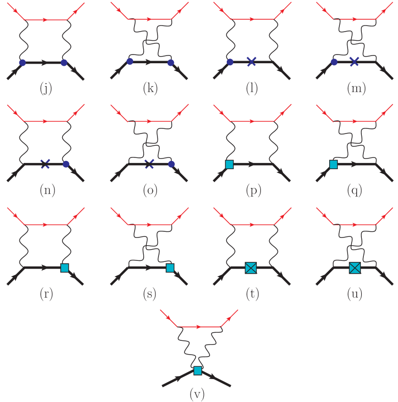
Figure 4: The subset of the NNLO TPE diagrams of $\mathcal{O}(\alpha^{2}/M^{2})$ contributing to our $\mathcal{O}(\alpha^{3}/M^{2})$ elastic differential cross-section. The thick, thin, and wiggly lines denote the proton, lepton, and photon propagators. The circular blobs represent insertions of NLO proton-photon vertices and the crosses represent ${\mathcal{O}}(1/M)$ proton propagators. The square blobs represent the insertions of renormalized NNLO proton-photon effective vertices and those with crosses represent ${\mathcal{O}}(1/M^{2})$ proton propagator terms.

In particular, for the diagrams (p)-(s) with the NNLO proton-photon vertex insertion, only the $\mathcal{O}(1/M^{2})$ part of the amplitudes are taken into consideration, omitting possible $\mathcal{O}(1/M^{3})$ terms. Again, as in the two previous orders, some of the terms proportional to $v_{\mu}v_{\nu}$ cancel between the amplitudes $\mathcal{M}^{(j)}_{\rm box}$, $\mathcal{M}^{(k)}_{\rm xbox}$, $\mathcal{M}^{(l)}_{\rm box}$, $\mathcal{M}^{(m)}_{\rm xbox}$, $\mathcal{M}^{(n)}_{\rm box}$, $\mathcal{M}^{(o)}_{\rm xbox}$, $\mathcal{M}^{(t)}_{\rm box}$ and $\mathcal{M}^{(u)}_{\rm xbox}$, where we use $v\cdot p_{p}=0$ (lab frame) and $v\cdot p^{\prime}_{p}=-\frac{Q^{2}}{2M}$ which contribute at ${\cal O}(1/M^{3})$, and hence, dropped to NNLO. In particular, the amplitudes for $\mathcal{M}^{(t)}_{\rm box}$ and $\mathcal{M}^{(u)}_{\rm xbox}$ cancel completely when adding the $v_{\mu}v_{\nu}$ terms. The non-vanishing, reduced amplitudes (using $p^{\prime}_{p}=Q$ in lab-frame) are given as

$${\widetilde{\mathcal{M}}^{(j)}_{\rm box}}\!\! = \!\!\frac{e^{4}}{4M^{2}}\int\frac{{\rm d}^{4}k}{(2\pi)^{4}i}\frac{\left[\bar{u}(p^{\prime})\gamma^{\mu}(\not{p}-\not{k}+m_{l})\gamma^{\nu}u(p)\right]}{(k^{2}+i0)\,[(Q-k)^{2}+i0]\,(k^{2}-2k\cdot p+i0)\,(v\cdot k+i0)}$$ (64)

$$\hskip 28.45274pt\times\left[\chi^{\dagger}(p^{\prime}_{p})\Big{\{}(Q+k)_{\mu}k_{\nu}-v_{\mu}k_{\nu}[v\cdot(Q+k)]-(Q+k)_{\mu}v_{\nu}(v\cdot k)\Big{\}}\chi(p_{p})\right]\,,$$

$${\widetilde{\mathcal{M}}^{(k)}_{\rm xbox}}\!\! = \!\!\frac{e^{4}}{4M^{2}}\int\frac{{\rm d}^{4}k}{(2\pi)^{4}i}\frac{\left[\bar{u}(p^{\prime})\gamma^{\mu}(\not{p}+\not{k}-\not{Q}+m_{l})\gamma^{\nu}u(p)\right]}{(k^{2}+i0)\,[(Q-k)^{2}+i0]\,(k^{2}+2k\cdot p^{\prime}+i0)\,(v\cdot k+i0)}$$ (65)

$$\hskip 28.45274pt\times\left[\chi^{\dagger}(p^{\prime}_{p})\Big{\{}k_{\mu}(Q+k)_{\nu}-k_{\mu}v_{\nu}[v\cdot(Q+k)]-v_{\mu}(Q+k)_{\nu}(v\cdot k)\Big{\}}\chi(p_{p})\right]\,,$$

$${\widetilde{\mathcal{M}}^{(l)}_{\rm box}}\!\! = \!\!\frac{e^{4}}{4M^{2}}\int\frac{{\rm d}^{4}k}{(2\pi)^{4}i}\frac{\left[\bar{u}(p^{\prime})\gamma^{\mu}(\not{p}-\not{k}+m_{l})\gamma^{\nu}u(p)\right]\Big{[}\chi^{\dagger}(p^{\prime}_{p})v_{\mu}k_{\nu}\chi(p_{p})\Big{]}}{(k^{2}+i0)\,[(Q-k)^{2}+i0]\,(k^{2}-2k\cdot p+i0)}\left(1-\frac{k^{2}}{(v\cdot k+i0)^{2}}\right)\,,$$ (66)

$${\widetilde{\mathcal{M}}^{(m)}_{\rm xbox}}\!\! = \!\!\frac{e^{4}}{4M^{2}}\int\frac{{\rm d}^{4}k}{(2\pi)^{4}i}\frac{\left[\bar{u}(p^{\prime})\gamma^{\mu}(\not{p}+\not{k}-\not{Q}+m_{l})\gamma^{\nu}u(p)\right]\Big{[}\chi^{\dagger}(p^{\prime}_{p})k_{\mu}v_{\nu}\chi(p_{p})\Big{]}}{(k^{2}+i0)\,[(Q-k)^{2}+i0]\,(k^{2}+2k\cdot p^{\prime}+i0)}\left(1-\frac{k^{2}}{(v\cdot k+i0)^{2}}\right)\,,$$ (67)

$${\widetilde{\mathcal{M}}^{(n)}_{\rm box}}\!\! = \!\!\frac{e^{4}}{4M^{2}}\int\frac{{\rm d}^{4}k}{(2\pi)^{4}i}\frac{\left[\bar{u}(p^{\prime})\gamma^{\mu}(\not{p}-\not{k}+m_{l})\gamma^{\nu}u(p)\right]\Big{[}\chi^{\dagger}(p^{\prime}_{p})(Q+k)_{\mu}v_{\nu}\chi(p_{p})\Big{]}}{(k^{2}+i0)\,[(Q-k)^{2}+i0]\,(k^{2}-2k\cdot p+i0)}\left(1-\frac{k^{2}}{(v\cdot k+i0)^{2}}\right)$$ (68)

$$+\,\frac{e^{4}}{4M^{2}}\int\frac{{\rm d}^{4}k}{(2\pi)^{4}i}\frac{\left[\bar{u}(p^{\prime})\gamma^{\mu}(\not{p}-\not{k}+m_{l})\gamma^{\nu}u(p)\right]\Big{[}\chi^{\dagger}(p^{\prime}_{p})v_{\mu}v_{\nu}\chi(p_{p})\Big{]}}{(k^{2}+i0)\,[(Q-k)^{2}+i0]\,(k^{2}-2k\cdot p+i0)}\cdot\frac{k^{2}}{(v\cdot k+i0)}\,,$$

$${\widetilde{\mathcal{M}}^{(o)}_{\rm xbox}}\!\! = \!\!\frac{e^{4}}{4M^{2}}\int\frac{{\rm d}^{4}k}{(2\pi)^{4}i}\frac{\left[\bar{u}(p^{\prime})\gamma^{\mu}(\not{p}+\not{k}-\not{Q}+m_{l})\gamma^{\nu}u(p)\right]\Big{[}\chi^{\dagger}(p^{\prime}_{p})v_{\mu}(Q+k)_{\nu}\chi(p_{p})\Big{]}}{(k^{2}+i0)\,[(Q-k)^{2}+i0]\,(k^{2}+2k\cdot p^{\prime}+i0)}\left(1-\frac{k^{2}}{(v\cdot k+i0)^{2}}\right)$$ (69)

$$+\,\frac{e^{4}}{4M^{2}}\int\frac{{\rm d}^{4}k}{(2\pi)^{4}i}\frac{\left[\bar{u}(p^{\prime})\gamma^{\mu}(\not{p}+\not{k}-\not{Q}+m_{l})\gamma^{\nu}u(p)\right]\Big{[}\chi^{\dagger}(p^{\prime}_{p})v_{\mu}v_{\nu}\chi(p_{p})\Big{]}}{(k^{2}+i0)\,[(Q-k)^{2}+i0]\,(k^{2}+2k\cdot p^{\prime}+i0)}\cdot\frac{k^{2}}{(v\cdot k+i0)}\,.$$

Since terms proportional to $v_{\mu}v_{\nu}$ do not cancel for the amplitudes (p)-(s), as well as in the seagull amplitude (v), their expressions are left unmodified. Next, we implement SPA for all the NNLO box and crossed-box diagrams which are explicit functions of the four-point loop-integrals. In contrast, the seagull diagram (v), being a three-point loop-function will be evaluated exactly without implementing SPA. We find that the NNLO box and crossed-box amplitudes factorize either into the LO Born amplitude $\mathcal{M}^{(0)}_{\gamma}$, Eq. (LABEL:eq:M0_LO), or the NLO amplitude $\mathcal{N}^{(1)}_{\gamma}$, Eq. (35), to yield the following reduced amplitudes with each being the sum of 2- and 3-point functions:

$${\widetilde{\mathcal{M}}^{(j)}_{\rm box}} \stackrel{{\scriptstyle\gamma_{\rm soft}}}{{\leadsto}} \frac{e^{2}E}{2M}{\mathcal{N}}^{(1)}_{\gamma}\!\!\int\frac{{\rm d}^{4}k}{(2\pi)^{4}i}\frac{1}{(k^{2}+i0)\,(k^{2}-2k\cdot p+i0)}+\frac{e^{2}E^{\prime}}{2M}{\mathcal{N}}^{(1)}_{\gamma}\!\!\int\frac{{\rm d}^{4}k}{(2\pi)^{4}i}\frac{1}{[(Q-k)^{2}+i0]\,(k^{2}-2k\cdot p+i0)}$$ (70)

$$+\,\frac{e^{2}Q^{2}}{2M}{\mathcal{N}}^{(1)}_{\gamma}\int\frac{{\rm d}^{4}k}{(2\pi)^{4}i}\frac{1}{[(Q-k)^{2}+i0]\,(k^{2}-2k\cdot p+i0)\,(v\cdot k+i0)}$$

$$-\,\frac{e^{2}Q^{2}}{2M^{2}}{\mathcal{M}}^{(0)}_{\gamma}\int\frac{{\rm d}^{4}k}{(2\pi)^{4}i}\frac{1}{[(Q-k)^{2}+i0]\,(k^{2}-2k\cdot p+i0)}+\mathcal{O}\left(\frac{1}{M^{3}}\right)\,,$$

$${\widetilde{\mathcal{M}}^{(k)}_{\rm xbox}} \stackrel{{\scriptstyle\gamma_{\rm soft}}}{{\leadsto}} \frac{e^{2}E^{\prime}}{2M}{\mathcal{N}}^{(1)}_{\gamma}\!\!\int\frac{{\rm d}^{4}k}{(2\pi)^{4}i}\frac{1}{(k^{2}+i0)\,(k^{2}+2k\cdot p^{\prime}+i0)}+\frac{e^{2}E}{2M}{\mathcal{N}}^{(1)}_{\gamma}\!\!\int\frac{{\rm d}^{4}k}{(2\pi)^{4}i}\frac{1}{[(Q-k)^{2}+i0]\,(k^{2}+2k\cdot p^{\prime}+i0)}$$ (71)

$$-\,\frac{e^{2}Q^{2}}{2M}{\mathcal{N}}^{(1)}_{\gamma}\int\frac{{\rm d}^{4}k}{(2\pi)^{4}i}\frac{1}{[(Q-k)^{2}+i0]\,(k^{2}+2k\cdot p^{\prime}+i0)\,(v\cdot k+i0)}$$

$$+\,\frac{e^{2}Q^{2}}{2M^{2}}{\mathcal{M}}^{(0)}_{\gamma}\int\frac{{\rm d}^{4}k}{(2\pi)^{4}i}\frac{1}{[(Q-k)^{2}+i0]\,(k^{2}+2k\cdot p^{\prime}+i0)}+\mathcal{O}\left(\frac{1}{M^{3}}\right)\,,$$

$${\widetilde{\mathcal{M}}^{(l)}_{\rm box}} \stackrel{{\scriptstyle\gamma_{\rm soft}}}{{\leadsto}} -\,\frac{e^{2}E^{\prime}}{2M}{\mathcal{N}}^{(1)}_{\gamma}\int\frac{{\rm d}^{4}k}{(2\pi)^{4}i}\frac{1}{[(Q-k)^{2}+i0]\,(k^{2}-2k\cdot p+i0)}\,,$$ (72)

$$+\,\frac{e^{2}Q^{2}E^{\prime}}{2M}{\mathcal{N}}^{(1)}_{\gamma}\int\frac{{\rm d}^{4}k}{(2\pi)^{4}i}\frac{1}{[(Q-k)^{2}+i0]\,(k^{2}-2k\cdot p+i0)\,(v\cdot k+i0)^{2}}\,,$$

$${\widetilde{\mathcal{M}}^{(m)}_{\rm xbox}} \stackrel{{\scriptstyle\gamma_{\rm soft}}}{{\leadsto}} -\,\frac{e^{2}E}{2M}{\mathcal{N}}^{(1)}_{\gamma}\int\frac{{\rm d}^{4}k}{(2\pi)^{4}i}\frac{1}{[(Q-k)^{2}+i0]\,(k^{2}+2k\cdot p^{\prime}+i0)}\,,$$ (73)

$$+\,\frac{e^{2}Q^{2}E}{2M}{\mathcal{N}}^{(1)}_{\gamma}\int\frac{{\rm d}^{4}k}{(2\pi)^{4}i}\frac{1}{[(Q-k)^{2}+i0]\,(k^{2}+2k\cdot p^{\prime}+i0)\,(v\cdot k+i0)^{2}}\,,$$

$${\widetilde{\mathcal{M}}^{(n)}_{\rm box}} \stackrel{{\scriptstyle\gamma_{\rm soft}}}{{\leadsto}} -\frac{e^{2}E}{2M}{\mathcal{N}}^{(1)}_{\gamma}\!\!\int\frac{{\rm d}^{4}k}{(2\pi)^{4}i}\frac{1}{(k^{2}+i0)\,(k^{2}-2k\cdot p+i0)}+\frac{e^{2}Q^{2}}{2M^{2}}{\mathcal{M}}^{(0)}_{\gamma}\!\!\int\frac{{\rm d}^{4}k}{(2\pi)^{4}i}\frac{1}{[(Q-k)^{2}+i0]\,(k^{2}-2k\cdot p+i0)}$$ (74)

$$-\,\frac{e^{2}Q^{4}}{2M^{2}}{\mathcal{M}}^{(0)}_{\gamma}\int\frac{{\rm d}^{4}k}{(2\pi)^{4}i}\frac{1}{[(Q-k)^{2}+i0]\,(k^{2}-2k\cdot p+i0)\,(v\cdot k+i0)^{2}}$$

$$-\,\frac{e^{2}Q^{2}E^{\prime}}{2M^{2}}{\mathcal{M}}^{(0)}_{\gamma}\int\frac{{\rm d}^{4}k}{(2\pi)^{4}i}\frac{1}{[(Q-k)^{2}+i0]\,(k^{2}-2k\cdot p+i0)\,(v\cdot k+i0)}\,,$$

$${\widetilde{\mathcal{M}}^{(o)}_{\rm xbox}} \stackrel{{\scriptstyle\gamma_{\rm soft}}}{{\leadsto}} -\frac{e^{2}E^{\prime}}{2M}{\mathcal{N}}^{(1)}_{\gamma}\!\!\int\frac{{\rm d}^{4}k}{(2\pi)^{4}i}\frac{1}{(k^{2}+i0)\,(k^{2}+2k\cdot p^{\prime}+i0)}-\frac{e^{2}Q^{2}}{2M^{2}}{\mathcal{M}}^{(0)}_{\gamma}\!\!\int\frac{{\rm d}^{4}k}{(2\pi)^{4}i}\frac{1}{[(Q-k)^{2}+i0]\,(k^{2}+2k\cdot p^{\prime}+i0)}$$ (75)

$$+\,\frac{e^{2}Q^{4}}{2M^{2}}{\mathcal{M}}^{(0)}_{\gamma}\int\frac{{\rm d}^{4}k}{(2\pi)^{4}i}\frac{1}{[(Q-k)^{2}+i0]\,(k^{2}+2k\cdot p^{\prime}+i0)\,(v\cdot k+i0)^{2}}$$

$$-\,\frac{e^{2}Q^{2}E}{2M^{2}}{\mathcal{M}}^{(0)}_{\gamma}\int\frac{{\rm d}^{4}k}{(2\pi)^{4}i}\frac{1}{[(Q-k)^{2}+i0]\,(k^{2}+2k\cdot p^{\prime}+i0)\,(v\cdot k+i0)}\,,$$

$${\mathcal{M}}^{(p)}_{\rm box} \stackrel{{\scriptstyle\gamma_{\rm soft}}}{{\leadsto}} -\,2e^{2}Q^{2}E\left(\frac{\langle r_{1}^{2}\rangle}{6}+\frac{\kappa_{p}}{4M^{2}}\right)\mathcal{M}_{\gamma}^{(0)}\int\frac{{\rm d}^{4}k}{(2\pi)^{4}i}\frac{1}{(k^{2}+i0)\,(k^{2}-2k\cdot p+i0)\,(v\cdot k+i0)}$$ (76)

$$-\,2e^{2}Q^{2}E^{\prime}\left(\frac{\langle r_{1}^{2}\rangle}{6}+\frac{\kappa_{p}}{4M^{2}}\right)\mathcal{M}_{\gamma}^{(0)}\int\frac{{\rm d}^{4}k}{(2\pi)^{4}i}\frac{1}{[(Q-k)^{2}+i0]\,(k^{2}-2k\cdot p+i0)\,(v\cdot k+i0)}+\mathcal{O}\left(\frac{1}{M^{3}}\right),\,\,$$

$${\mathcal{M}}^{(q)}_{\rm xbox} \stackrel{{\scriptstyle\gamma_{\rm soft}}}{{\leadsto}} -\,2e^{2}Q^{2}E\left(\frac{\langle r_{1}^{2}\rangle}{6}+\frac{\kappa_{p}}{4M^{2}}\right)\mathcal{M}_{\gamma}^{(0)}\int\frac{{\rm d}^{4}k}{(2\pi)^{4}i}\frac{1}{[(Q-k)^{2}+i0]\,(k^{2}+2k\cdot p^{\prime}+i0)\,(v\cdot k+i0)}$$ (77)

$$-\,2e^{2}Q^{2}E^{\prime}\left(\frac{\langle r_{1}^{2}\rangle}{6}+\frac{\kappa_{p}}{4M^{2}}\right)\mathcal{M}_{\gamma}^{(0)}\int\frac{{\rm d}^{4}k}{(2\pi)^{4}i}\frac{1}{(k^{2}+i0)\,(k^{2}+2k\cdot p^{\prime}+i0)\,(v\cdot k+i0)}+\mathcal{O}\left(\frac{1}{M^{3}}\right)\,,$$

$${\mathcal{M}}^{(r)}_{\rm box} \stackrel{{\scriptstyle\gamma_{\rm soft}}}{{\leadsto}} -\,2e^{2}Q^{2}E\left(\frac{\langle r_{1}^{2}\rangle}{6}+\frac{\kappa_{p}}{4M^{2}}\right)\mathcal{M}_{\gamma}^{(0)}\int\frac{{\rm d}^{4}k}{(2\pi)^{4}i}\frac{1}{(k^{2}+i0)\,(k^{2}-2k\cdot p+i0)\,(v\cdot k+i0)}$$ (78)

$$-\,2e^{2}Q^{2}E^{\prime}\left(\frac{\langle r_{1}^{2}\rangle}{6}+\frac{\kappa_{p}}{4M^{2}}\right)\mathcal{M}_{\gamma}^{(0)}\int\frac{{\rm d}^{4}k}{(2\pi)^{4}i}\frac{1}{[(Q-k)^{2}+i0]\,(k^{2}-2k\cdot p+i0)\,(v\cdot k+i0)}+\mathcal{O}\left(\frac{1}{M^{3}}\right),\,\,$$

$${\mathcal{M}}^{(s)}_{\rm xbox} \stackrel{{\scriptstyle\gamma_{\rm soft}}}{{\leadsto}} -\,2e^{2}Q^{2}E\left(\frac{\langle r_{1}^{2}\rangle}{6}+\frac{\kappa_{p}}{4M^{2}}\right)\mathcal{M}_{\gamma}^{(0)}\int\frac{{\rm d}^{4}k}{(2\pi)^{4}i}\frac{1}{[(Q-k)^{2}+i0]\,(k^{2}+2k\cdot p^{\prime}+i0)\,(v\cdot k+i0)}$$ (79)

$$-\,2e^{2}Q^{2}E^{\prime}\left(\frac{\langle r_{1}^{2}\rangle}{6}+\frac{\kappa_{p}}{4M^{2}}\right)\mathcal{M}_{\gamma}^{(0)}\int\frac{{\rm d}^{4}k}{(2\pi)^{4}i}\frac{1}{(k^{2}+i0)\,(k^{2}+2k\cdot p^{\prime}+i0)\,(v\cdot k+i0)}+\mathcal{O}\left(\frac{1}{M^{3}}\right)\,.$$

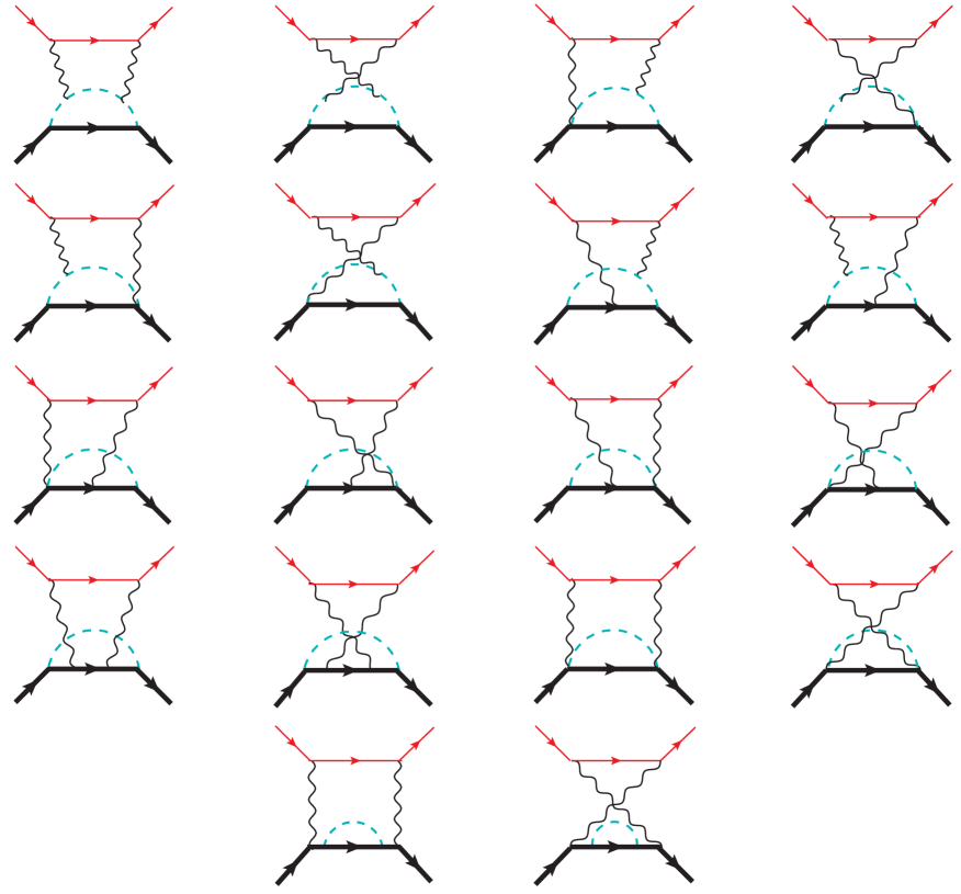
Figure 5: The subset of two-loop NNLO TPE diagrams of $\mathcal{O}(\alpha^{2}/M^{2})$ with non-factorizable pion-loops, which in principle contribute to the $\mathcal{O}(\alpha^{3}/M^{2})$ elastic differential cross-section. The thick and thin solid lines denote the proton and lepton propagators, whereas the dashed and wiggly lines denote the pion and photon propagators. To one-loop approximation in the perturbative expansion, the contribution from these diagrams in combination with the appropriate counter-term diagrams are excluded in our analysis since they are expected to yield rather tiny contributions.

Hence, the sum of the NNLO amplitudes can be summarized as

$$\mathcal{M}_{\gamma\gamma}^{(jkl\cdots v)}\!\! = \!\!\widetilde{\mathcal{M}}_{\rm box}^{(j)}+\widetilde{\mathcal{M}}_{\rm xbox}^{(k)}+\widetilde{\mathcal{M}}_{\rm box}^{(l)}+\widetilde{\mathcal{M}}_{\rm xbox}^{(m)}+\widetilde{\mathcal{M}}_{\rm box}^{(n)}+\widetilde{\mathcal{M}}_{\rm xbox}^{(o)}+{\mathcal{M}}_{\rm box}^{(p)}+{\mathcal{M}}_{\rm xbox}^{(q)}+{\mathcal{M}}_{\rm box}^{(r)}+{\mathcal{M}}_{\rm xbox}^{(s)}+{\mathcal{M}^{(\rm v)}_{\rm seagull}}$$ (80)

$$\stackrel{{\scriptstyle\gamma_{\rm soft}}}{{\leadsto}} \mathcal{M}_{\gamma}^{(0)}f^{(jkl\cdots u)}_{\gamma\gamma}(Q^{2})+{\mathcal{M}^{(v)}_{\rm seagull}}\,,\qquad\text{where}$$

$$f^{(jkl\cdots u)}_{\gamma\gamma}(Q^{2})\!\! = \!\!-\,\frac{e^{2}Q^{2}}{2M^{2}}\bigg{\{}E^{\prime}\bcancel{I^{-}(p,0|0,1,1,1)}+E\bcancel{I^{+}(p^{\prime},0|0,1,1,1)}+Q^{2}I^{-}(p,0|0,1,1,2)-Q^{2}I^{+}(p^{\prime},0|0,1,1,2)\bigg{\}}$$ (81)

$$\!\!+\,\frac{e^{2}Q^{2}{\mathcal{M}}^{(0)*}_{\gamma}{\mathcal{N}}^{(1)}_{\gamma}}{2M\left|{\mathcal{M}}^{(0)}_{\gamma}\right|^{2}}\bigg{\{}I^{-}(p,0|0,1,1,1)-I^{+}(p^{\prime},0|0,1,1,1)+E^{\prime}I^{-}(p,0|0,1,1,2)+EI^{+}(p,0|0,1,1,2)\bigg{\}}$$

$$\!\!-\,4e^{2}Q^{2}\left(\frac{\langle r_{1}^{2}\rangle}{6}+\frac{\kappa_{p}}{4M^{2}}\right)\bigg{\{}E\cancel{I^{-}(p,0|1,0,1,1)}+E^{\prime}\cancel{I^{+}(p^{\prime},0|1,0,1,1)}+E^{\prime}\bcancel{I^{-}(p,0|0,1,1,1)}$$

$$\hskip 110.96556pt+E\bcancel{I^{+}(p^{\prime},0|0,1,1,1)\bigg{\}}}+{\mathcal{O}}\left(\frac{1}{M^{3}}\right)\,.$$

The loop-integrals in the above expression already appeared in the NLO amplitude $f^{(cde\cdots h)}_{\gamma\gamma}$, Eq. (II.2) whose analytical expressions of ${\mathcal{O}}(1/M^{2})$ are provided in the appendix. Just as in the NLO case, the IR-divergent integrals $I^{-}(p,0|1,0,1,1)$ and $I^{+}(p^{\prime},0|1,0,1,1)$ do not contribute to the cross-section since the pre-factor ${\mathcal{M}}^{(0)*}_{\gamma}{\mathcal{N}}^{(1)}_{\gamma}$ causes the entire second-line expression in Eq. (81) to vanish identically when calculating the elastic cross-section. Moreover, in this work, since we intend to preserve the accuracy of all analytical expressions to $\mathcal{O}(1/M^{2})$, it is legitimate at this point to substitute $E=E^{\prime}$ and $\beta=\beta^{\prime}$ in all terms of $\mathcal{O}(1/M^{2})$. Consequently, with the integrals $I^{-}(p,0|0,1,1,1)$ and $I^{-}(p,0|1,0,1,1)$ effectively canceling with $I^{+}(p^{\prime},0|0,1,1,1)$ and $I^{+}(p^{\prime},0|1,0,1,1)$, respectively, the proton’s structure effects in TPE drop out up to $\mathcal{O}(1/M^{2})$. The only terms in the amplitude that will effectively contribute to the cross-section are the 3-point integral functions $I^{-}(p,0|0,1,1,2)$ and $I^{+}(p^{\prime},0|0,1,1,2)$ appearing in the first line of $f^{(jkl\cdots u)}_{\gamma\gamma}$, Eq. (81). Notably, as seen from the $\mathcal{O}(1/M^{2})$ expressions of these 3-point functions provided in the appendix, they are each of $\mathcal{O}(M)$, and therefore, generate kinematically enhanced contributions of $\mathcal{O}(1/M)$ to the amplitude $f^{(jkl\cdots u)}_{\gamma\gamma}$ which do not cancel.

Finally, the $\mathcal{O}(\alpha/M^{2})$ fractional contribution (relative to the LO) to the elastic differential cross-section from the NNLO diagrams are collected within the term

$$\delta^{(jkl\cdots v)}_{\gamma\gamma}(Q^{2})\!\! = \!\!\frac{2{\mathcal{R}}e\sum\limits_{spins}\left[\mathcal{M}_{\gamma}^{(0)*}{\mathcal{M}}_{\gamma\gamma}^{(jkl\cdots v)}\right]}{\sum\limits_{spins}\left|\mathcal{M}_{\gamma}^{(0)}\right|^{2}}$$ (82)

$$= \!\!\delta^{(jkl\cdots u)}_{\gamma\gamma}(Q^{2})+\delta_{\gamma\gamma;{\rm NNLO}}^{\rm(seagull)}(Q^{2})\,,$$

where the contributions from the TPE box and crossed-box diagrams (j)-(u), and the NNLO seagull diagram (v), are respectively, given as

$$\delta^{(jkl\cdots u)}_{\gamma\gamma}(Q^{2})\!\! \stackrel{{\scriptstyle\gamma_{\rm soft}}}{{\leadsto}} \!\!\frac{2\alpha Q^{2}}{\pi ME\beta}\ln{\sqrt{\frac{1+\beta}{1-\beta}}}+\frac{\alpha Q^{4}}{2\pi M^{2}E^{2}\beta^{3}}\left(\beta-\ln{\sqrt{\frac{1+\beta}{1-\beta}}}\,\,\right)+{\mathcal{O}}\left(\frac{1}{M^{3}}\right)\,,\quad\text{and}$$ (83)

$$\delta_{\gamma\gamma;{\rm NNLO}}^{\rm(seagull)}(Q^{2})\!\! = \!\!\frac{\pi\alpha Q^{2}}{4M^{2}}{\mathcal{R}}e\bigg{\{}\cancel{2Q\cdot I^{-}_{1}(p,0|1,1,1,0)}-\cancel{Q^{2}I(Q|1,1,1,0)}\bigg{\}}+{\mathcal{O}}\left(\frac{1}{M^{3}}\right)\sim{\mathcal{O}}\left(\frac{1}{M^{3}}\right)\,,$$ (84)

where, as said, the seagull terms have been evaluated exactly. Besides, they yield kinematically suppressed terms of ${\mathcal{O}}\left(1/M^{3}\right)$, which are dropped from our analytical results with the intended accuracy of ${\mathcal{O}}\left(1/M^{2}\right)$. Thus, on the one hand, we see that the contributions arising from the NNLO seagull diagram (v), as well as the proton’s structure-dependent form factor diagrams (p)-(s), are all of ${\mathcal{O}}\left(1/M^{3}\right)$ [cf. Eq. (84) and the last line of Eq. (81)], namely, beyond our working accuracy, and hence, excluded from our results. On the other hand, it is interesting to find a kinematically enhanced ${\mathcal{O}}\left(1/M\right)$ term in our NNLO expression of $\delta^{(jkl\cdots u)}_{\gamma\gamma}$ which is formally commensurate with NLO. This is attributed to the contribution of the 3-point function $I^{(0)}(p,0|0,1,1,2)\sim{\mathcal{O}}(M)$ constituting the leading order part of the loop-integrals $I^{-}(p,0|0,1,1,2)$ and $I^{+}(p^{\prime},0|0,1,1,2)$ whose expressions are provided in the appendix. Therefore, the only proton’s structure-dependent contributions at this order can potentially arise from the non-factorizable two-loop (i.e., a photon loop and a pion-loop) diagrams (cf. Fig. 5), along with appropriate counter-terms, which we have excluded in our analysis owing to the rather intricate nature of their analytical evaluations necessary to express their contributions to the cross-sections in algebraic closed form. In a naive perturbative counting scheme, such two-loop contributions are expected to be subdominant compared to their one-loop counterparts. Nonetheless, this calls for a more rigorous systematic evaluation of the TPE including all NNLO contributions, without recourse to any type of approximations, including SPA. Such an endeavor is a subject matter for a future publication.

II.4 A Summary of the TPE Expression

In the lab-frame the total fractional TPE contribution (relative to the LO) including up to the ${\mathcal{O}}(\alpha/M^{2})$ or NNLO corrections to the unpolarized $\ell$-p elastic differential cross-section, after isolating the residual ${\mathcal{O}}(1/M)$ IR-divergence $\delta^{\rm(box)}_{\rm IR}$ from diagrams (a) and (b), Eq. (20), is given by

$$\overline{\delta^{\rm(TPE)}_{\gamma\gamma}}(Q^{2})\!\! = \!\!\frac{2{\mathcal{R}}e\sum\limits_{spins}\left[\mathcal{M}_{\gamma}^{(0)*}\mathcal{M}_{\gamma\gamma}^{\rm(TPE)}\right]}{\sum\limits_{spins}\left|\mathcal{M}_{\gamma}^{(0)}\right|^{2}}-\delta^{\rm(box)}_{\rm IR}(Q^{2})\,.$$

With the sum of all the 22 TPE amplitudes (a)-(v), given by $\mathcal{M}_{\gamma\gamma}^{\rm(TPE)}={\mathcal{M}^{(a)}_{\rm box}}+\cdots+{\mathcal{M}^{(v)}_{\rm seagull}}$, the total IR-finite part of the TPE contributions can be expressed as

$$\overline{\delta^{\rm(TPE)}_{\gamma\gamma}}(Q^{2})\!\! = \!\!\delta^{\rm(LO)}_{\gamma\gamma}(Q^{2})+\delta^{\rm(NLO)}_{\gamma\gamma}(Q^{2})$$ (86)

$$\!\!+\,\delta^{\rm(NNLO)}_{\gamma\gamma}(Q^{2})+{\mathcal{O}}\left(M^{-3}\right)\,,$$

where $\delta^{\rm(LO)}_{\gamma\gamma}\sim{\mathcal{O}}(M^{0})$, $\delta^{\rm(NLO)}_{\gamma\gamma}\sim{\mathcal{O}}(1/M)$ and $\delta^{\rm(NNLO)}_{\gamma\gamma}\sim{\mathcal{O}}(1/M^{2})$. As mentioned earlier, our TPE evaluation employing SPA runs into a technical problem, namely, that the strict LO [i.e., ${\mathcal{O}}(M^{0})$] contribution vanishes completely, thereby potentially spoiling the HB$\chi$PT power counting with a non-vanishing NLO contribution. To rectify this artifact, we have, therefore, included the exact LO TPE result, Eq. (18), taken from the recent work Choudhary:2023rsz on the exact analytical TPE evaluation:

$$\delta^{\rm(LO)}_{\gamma\gamma}(Q^{2})=\delta^{\rm(0)}_{\gamma\gamma}(Q^{2})=\pi\alpha\frac{\sqrt{-Q^{2}}}{2E}\left(\frac{1}{1+\frac{Q^{2}}{4E^{2}}}\right)\,.$$ (87)

Next, by collecting all the NLO [i.e., ${\mathcal{O}}(1/M)$] contributions from Eqs. (19), (46), (II.2) and (83), yields our total NLO fractional TPE contributions to the elastic cross-section, relative to the LO Born term [cf. Eq. (91)]:

$$\delta^{\rm(NLO)}_{\gamma\gamma}(Q^{2}) \stackrel{{\scriptstyle\gamma_{\rm soft}}}{{\leadsto}} -\frac{\alpha Q^{2}}{\pi ME\beta^{2}}\Bigg{[}1+\frac{\pi^{2}}{12}\left(\beta+\frac{1}{\beta}\right)+(1-\beta)\ln\sqrt{\frac{1+\beta}{1-\beta}}-2\ln\sqrt{\frac{2\beta}{1-\beta}}-2\ln\sqrt{-\frac{Q^{2}}{2ME\beta}}$$ (88)

$$\hskip 49.79231pt+\,2\left(\beta+\frac{1}{\beta}\right)\ln\sqrt{-\frac{Q^{2}}{2ME\beta}}\ln\sqrt{\frac{1+\beta}{1-\beta}}-\frac{1}{2}\left(3\beta+\frac{1}{\beta}\right)\ln^{2}\sqrt{\frac{1+\beta}{1-\beta}}-\beta{\rm Li}_{2}\left(\frac{2\beta}{1+\beta}\right)$$

$$\hskip 49.79231pt-\,\frac{1}{2}\left(\beta+\frac{1}{\beta}\right){\rm Li}_{2}\left(\frac{1+\beta}{1-\beta}\right)\Bigg{]}-\frac{4\alpha E}{\pi M}\left[\frac{Q^{2}}{Q^{2}+4E^{2}}\right]\left(\frac{\nu_{l}^{2}-1}{\nu_{l}^{2}}\right)\Bigg{[}\left(\frac{1+\nu_{l}^{2}}{2\nu_{l}}\right)\bigg{\{}\frac{\pi^{2}}{3}$$

$$\hskip 49.79231pt+\,\ln^{2}\sqrt{\frac{\nu_{l}+1}{\nu_{l}-1}}+{\rm Li}_{2}\left(\frac{\nu_{l}-1}{\nu_{l}+1}\right)\bigg{\}}-\ln\sqrt{-\frac{Q^{2}}{m_{l}^{2}}}\,\,\Bigg{]}\,.$$

Likewise, collecting all the NNLO [i.e., ${\mathcal{O}}(1/M^{2})$] contributions from Eqs. (19), (46), (II.2), (83) and (84), yields our NNLO fractional TPE contributions, relative to the LO Born term [cf. Eq. (91)]:

$$\delta^{\rm(NNLO)}_{\gamma\gamma}(Q^{2}) \stackrel{{\scriptstyle\gamma_{\rm soft}}}{{\leadsto}} \frac{\alpha Q^{4}}{8\pi M^{2}E^{2}\beta^{5}}\Bigg{[}\frac{\pi^{2}}{6}(3-\beta^{2})-18\beta+12\beta\ln{\sqrt{\frac{2\beta}{1-\beta}}}-\left(3+\beta^{2}\right)\ln^{2}{\sqrt{\frac{1+\beta}{1-\beta}}}-(3-\beta^{2})$$ (89)

$$\hskip 54.06006pt\times\,{\rm Li}_{2}\left(\frac{1+\beta}{1-\beta}\right)-2\beta^{2}{\rm Li}_{2}\left(\frac{2\beta}{1+\beta}\right)+2\ln{\sqrt{-\frac{Q^{2}}{2ME\beta}}}\left(6\beta+2(3-\beta^{2})\ln{\sqrt{\frac{1+\beta}{1-\beta}}}\,\right)$$

$$\hskip 54.06006pt\,-2\left(4+3\beta-\beta^{2}\right)\ln{\sqrt{\frac{1+\beta}{1-\beta}}}\,\,\Bigg{]}+\frac{8\alpha E^{2}}{\pi M^{2}}\bigg{[}\frac{Q^{2}}{Q^{2}+4E^{2}}\bigg{]}^{2}\left(\frac{\nu_{l}^{2}-1}{\nu_{l}^{2}}\right)\Bigg{[}\left(\frac{1+\nu_{l}^{2}}{2\nu_{l}}\right)\bigg{\{}\frac{\pi^{2}}{3}$$

$$\hskip 54.06006pt+\,\ln^{2}{\sqrt{\frac{\nu_{l}+1}{\nu_{l}-1}}}+{\rm Li}_{2}\left(\frac{\nu_{l}-1}{\nu_{l}+1}\right)\bigg{\}}-\ln\sqrt{-\frac{Q^{2}}{m_{l}^{2}}}\,\,\Bigg{]}-\frac{\alpha Q^{2}}{2\pi M^{2}\nu_{l}^{2}}\bigg{[}\frac{Q^{2}}{Q^{2}+4E^{2}}\bigg{]}\Bigg{[}\left(\frac{\nu_{l}^{2}-1}{\nu_{l}}\right)$$

$$\hskip 54.06006pt\times\,\bigg{\{}\frac{\pi^{2}}{3}+\ln^{2}{\sqrt{\frac{\nu_{l}+1}{\nu_{l}-1}}+{\rm Li}_{2}\left(\frac{\nu_{l}-1}{\nu_{l}+1}\right)}\bigg{\}}+2\ln\sqrt{-\frac{Q^{2}}{m_{l}^{2}}}\,\,\Bigg{]}+o\left(\frac{1}{M^{2}}\right)\,.$$

The $o\left(\frac{1}{M^{2}}\right)$ symbol  used above denotes all possible NNLO terms that may arise from the excluded non-factorizable two-loop contributions, as displayed in Fig. 5. The resultant magnitudes of the individual LO, NLO, and NNLO contributions, as well as their sum are shown in Fig. 6. Furthermore, in Fig. 7, we present a comparison our SPA-based TPE prediction with those of the earlier SPA works of Talukdar et al. Talukdar:2019dko ; Talukdar:2020aui , as well as the exact TPE prediction of Choudhary et al. Choudhary:2023rsz .

III Charge Asymmetry up to Next-to-leading Order

To evaluate the charge asymmetry to NLO accuracy, we include the HB$\chi$PT results for the various higher-order contributions (radiative and hadronic) to the unpolarized elastic lepton-proton scattering cross-section, along the SPA-based evaluated TPE results of Ref. Talukdar:2020aui . The differential cross-sections for lepton and anti-lepton scattering with the proton is expressed as

$$\frac{{\rm d}\sigma^{(\mp)}_{el}(Q^{2})}{{\rm d}\Omega^{\prime}_{l}}\!\! = \!\!\left[\frac{{\rm d}\sigma_{el}(Q^{2})}{{\rm d}\Omega^{\prime}_{l}}\right]_{0}$$ (90)

$$\times\,\left[1+\delta_{\rm even}(Q^{2})\pm\delta_{\rm odd}(Q^{2})\right]\,,$$

where the LO Born contribution is given by Talukdar:2020aui

$$\left[\frac{{\rm d}\sigma_{el}(Q^{2})}{{\rm d}\Omega^{\prime}_{l}}\right]_{0}\!\! = \!\!\frac{\alpha^{2}E^{\prime}\beta^{\prime}}{E\beta Q^{2}}\left(1-\frac{Q^{2}}{4M^{2}}\right)\left[1+\frac{4EE^{\prime}}{Q^{2}}\right]\,.\quad\,$$ (91)

Here, we recognize the charge-odd (charge-even) corrections $\pm\delta_{\rm odd}$ ($\delta_{\rm even}$), relative to the LO Born contribution, as those which change (do not change) signs when interchanging the polarities of the lepton charge. We first consider the parts of the TPE corrections up-to-and-including NLO expressed as

$$\widetilde{\delta}^{\rm(TPE)}_{\gamma\gamma}(Q^{2})\equiv\delta^{\rm(box)}_{\rm IR}(Q^{2})+\delta^{\rm(LO)}_{\gamma\gamma}(Q^{2})+\delta^{\rm(NLO)}_{\gamma\gamma}(Q^{2})\,.\quad\,$$ (92)

Next by adding the low-energy NLO charge-odd soft-photon bremsstrahlung corrections $\delta^{\rm(odd;\,1)}_{\gamma\gamma^{*}}\sim{\mathcal{O}}(1/M)$ which were evaluated in Ref. Talukdar:2020aui , we obtain our total charge-odd radiative corrections $\delta_{\rm odd}$ up to NLO accuracy, expressed in the form:

$$\delta_{\rm odd}(Q^{2})=\widetilde{\delta}^{\rm(TPE)}_{\gamma\gamma}(Q^{2})+\delta^{\rm(odd;\,1)}_{\gamma\gamma^{*}}(Q^{2})+o\left(\frac{1}{M^{3}}\right)\,,$$ (93)

where $o\left(\frac{1}{M^{3}}\right)$ denote neglected terms due to dynamical contributions from $N{}^{3}$LO charge-odd radiative corrections. The analytical expression for $\delta_{\rm odd}$ is given as

$$\delta^{\rm(odd;\,1)}_{\gamma\gamma^{*}}(Q^{2})\!\! = \!\!\delta^{\rm(soft)}_{\rm IR}(Q^{2})+\frac{2\alpha}{\pi\beta}\ln\sqrt{\frac{-Q^{2}}{m^{2}_{l}}}\left\{\ln{\sqrt{\frac{1+\beta}{1-\beta}}}-\frac{\beta}{\beta^{\prime}}\ln{\sqrt{\frac{1+\beta^{\prime}}{1-\beta^{\prime}}}}\,\right\}$$ (94)

$$-\,\frac{\alpha Q^{2}}{2\pi ME\beta}\left[\ln{\left(\frac{4\Delta^{2}_{\gamma^{*}}E^{2}}{-Q^{2}{E^{\prime}}^{2}}\right)}\ln{\sqrt{\frac{1+\beta}{1-\beta}}}-\frac{1}{2}{\rm Li}_{2}\left(\frac{2\beta}{1+\beta}\right)+\frac{1}{2}{\rm Li}_{2}\left(\frac{2\beta}{\beta-1}\right)\right]$$

$$-\,\frac{\alpha Q^{2}}{2\pi M\beta^{\prime}E^{\prime}}\left[\ln{\left(\frac{4\Delta^{2}_{\gamma^{*}}E^{2}}{-Q^{2}{E^{\prime}}^{2}}\right)}\ln{\sqrt{\frac{1+\beta^{\prime}}{1-\beta^{\prime}}}}-\frac{1}{2}{\rm Li}_{2}\left(\frac{2\beta^{\prime}}{1+\beta^{\prime}}\right)+\frac{1}{2}{\rm Li}_{2}\left(\frac{2\beta^{\prime}}{\beta^{\prime}-1}\right)\right]$$

$$+\,\frac{8\alpha\Delta_{\gamma^{*}}{E^{\prime}}^{2}}{\pi ME^{2}(Q^{2}+4EE^{\prime})}\Bigg{[}-\Delta_{\gamma^{*}}(E+E^{\prime})+\Delta_{\gamma^{*}}\frac{E^{2}}{E^{\prime}\beta^{\prime}}\left\{\left(1-\frac{\beta}{\beta^{\prime}}\right)\ln{\sqrt{\frac{1+\beta^{\prime}}{1-\beta^{\prime}}}}-\beta\right\}$$

$$\hskip 72.55461pt+\,\Delta_{\gamma^{*}}\frac{{E^{\prime}}^{2}}{E\beta}\left\{\left(1-\frac{\beta^{\prime}}{\beta}\right)\ln{\sqrt{\frac{1+\beta}{1-\beta}}}-\beta^{\prime}\right\}+\frac{1}{E\beta}\Bigg{\{}2m^{2}_{l}\left(\frac{EE^{\prime}-E^{\prime 2}}{E}\right)$$

$$\hskip 72.55461pt+\,\Delta_{\gamma^{*}}\left(m^{2}_{l}-\frac{1}{2}Q^{2}\right)\Bigg{\}}\left\{\ln{\sqrt{\frac{1+\beta}{1-\beta}}}-\frac{E\beta}{E^{\prime}\beta^{\prime}}\ln{\sqrt{\frac{1+\beta^{\prime}}{1-\beta^{\prime}}}}\,\right\}\Bigg{]}\,,$$

where the term $\delta^{\rm(soft)}_{\rm IR}$ constitutes the IR-divergent part of the charge-odd soft-photon bremsstrahlung contributions Talukdar:2020aui . This IR-divergence is exactly equal but of opposite sign to the TPE IR-divergent counterpart, i.e., $\delta^{\rm(soft)}_{\rm IR}=-\delta^{\rm(box)}_{\rm IR}$ [cf. Eq. (20)]. In other words, this implies that the two singular terms get eliminated in their sum in $\delta_{\rm odd}(Q^{2})$, Eq. (93). We should emphasize that the above result for the bremsstrahlung contributions borrowed from Ref. Talukdar:2020aui pertains to the use of the Coulomb gauge, whereas the TPE calculations invoking SPA in this work were carried out in the Lorentz gauge. Currently, work is in progress for a future publication Bhoomika24 , where we shall consider the bremsstrahlung calculations (both charge-even and -odd) adopting the Lorentz gauge at NLO accuracy. In this process, possible sources of systematic errors due to the mismatch between the different gauge-dependent terms should get eliminated. It is nonetheless important to stress that $\delta^{\rm(soft)}_{\rm IR}$ has precisely the same structure irrespective of the choice of the gauge. The NLO expression for the total charge-odd radiative correction $\delta_{\rm odd}$ in Eq. (93) includes the IR-finite combination of our SPA-based TPE corrections $\tilde{\delta}^{\rm(TPE)}_{\gamma\gamma}$, Eq. (92), as well as the associated charge-odd soft-photon bremsstrahlung counterparts $\delta^{\rm(odd;\,1)}_{\gamma\gamma^{*}}$, Eq. (94), considering all dynamical corrections terms up-to-and-including NLO.

We now consider the total LO charge-even radiative corrections (both real and virtual), $\delta^{\rm(even;\,0)}_{2\gamma}\sim{\mathcal{O}}(M^{0})$, as well as the leading hadronic corrections to the OPE, $\delta^{(2)}_{\chi}\sim{\mathcal{O}}(1/M^{2})$. Together, these constitute our total charge-even contributions $\delta_{\rm even}$ to NLO accuracy. Thus, we can express the charge-even contributions to the cross-section in the form:

$$\delta_{\rm even}(Q^{2})=\delta^{\rm(even;\,0)}_{2\gamma}(Q^{2})+\delta^{(2)}_{\chi}(Q^{2})+o\left(\frac{1}{M^{3}}\right)\,,$$ (95)

where $o\left(\frac{1}{M^{3}}\right)$ denotes neglected terms due to N³LO charge-even radiative corrections. Below, we spell out the analytical results of Ref. Talukdar:2020aui which we borrow in our work to obtain our results for the total charge-even fractional corrections. The following two results are considered:

First, the expression for NLO charge-even radiative corrections $\delta^{\rm(even;\,0)}_{2\gamma}$ is given by the following expression:

$$\delta^{\rm(even;\,0)}_{2\gamma}(Q^{2})\!\! = \!\!\frac{\alpha}{\pi}\Bigg{[}\frac{\nu_{l}^{2}+1}{4\nu_{l}}\ln{\left(\frac{\nu_{l}+1}{\nu_{l}-1}\right)}\ln{\left(\frac{\nu_{l}^{2}-1}{4\nu_{l}^{2}}\right)}+\frac{2\nu_{l}^{2}+1}{2\nu_{l}}\ln{\left(\frac{\nu_{l}+1}{\nu_{l}-1}\right)}-\frac{\nu_{l}^{2}+1}{2\nu_{l}}\bigg{\{}{\rm Li}_{2}\left(\frac{\nu_{l}-1}{2\nu_{l}}\right)-{\rm Li}_{2}\left(\frac{\nu_{l}+1}{2\nu_{l}}\right)\bigg{\}}$$ (96)

$$\hskip 11.38092pt-\,2+\sum_{f=e,\mu,\tau}\Bigg{\{}\frac{2}{3}\left(\nu_{f}^{2}-\frac{8}{3}\right)+\nu_{f}\left(\frac{3-\nu_{f}^{2}}{3}\right)\ln{\left(\frac{\nu_{f}+1}{\nu_{f}-1}\right)}\Bigg{\}}-\frac{2}{3}\left(\nu_{\pi}^{2}+\frac{1}{3}\right)+\frac{\nu_{\pi}^{2}}{3}\ln{\left(\frac{\nu_{\pi}+1}{\nu_{\pi}-1}\right)}$$

$$\hskip 11.38092pt+\,\frac{1}{\nu_{l}}\left(\frac{2m_{l}^{2}}{Q^{2}+4EE^{\prime}}\right)\left(1-\frac{Q^{2}}{4M^{2}}\right)\ln{\left(\frac{\nu_{l}+1}{\nu_{l}-1}\right)}+\ln{\left(\frac{4\Delta^{2}_{\gamma^{*}}E^{2}}{m_{l}^{2}E^{\prime 2}}\right)}\bigg{[}\frac{\nu_{l}^{2}+1}{2\nu_{l}}\ln{\left(\frac{\nu_{l}+1}{\nu_{l}-1}\right)}-1\bigg{]}$$

$$\hskip 11.38092pt+\,\frac{1}{\beta}\ln{\sqrt{\frac{1+\beta}{1-\beta}}}+\frac{1}{\beta^{\prime}}\ln{\sqrt{\frac{1+\beta^{\prime}}{1-\beta^{\prime}}}}-\frac{\nu_{l}^{2}+1}{2\nu_{l}}\Bigg{\{}\ln^{2}{\sqrt{\frac{1+\beta}{1-\beta}}}-\ln^{2}{\sqrt{\frac{1+\beta^{\prime}}{1-\beta^{\prime}}}}-{\rm Li}_{2}\left(1+\frac{E-\lambda_{\nu}E^{\prime}}{E^{\prime}(1-\beta^{\prime})\xi_{\nu}}\right)$$

$$\hskip 11.38092pt-\,{\rm Li}_{2}\left(1+\frac{E-\lambda_{\nu}E^{\prime}}{E^{\prime}(1+\beta^{\prime})\xi_{\nu}}\right)+{\rm Li}_{2}\left(1+\frac{E-\lambda_{\nu}E^{\prime}}{E(1-\beta)\lambda_{\nu}\xi_{\nu}}\right)+{\rm Li}_{2}\left(1+\frac{E-\lambda_{\nu}E^{\prime}}{E(1+\beta)\lambda_{\nu}\xi_{\nu}}\right)\Bigg{\}}\Bigg{]}\,,$$

where, the kinematic factors $\nu_{f},\nu_{\pi},\xi_{\nu}$, and $\lambda_{\nu}$, are respectively, defined as

$$\nu_{f}=\sqrt{1-\frac{4m^{2}_{f}}{Q^{2}}}\,,\quad\nu_{\pi}=\sqrt{1-\frac{4m^{2}_{\pi}}{Q^{2}}}\,,\quad\xi_{\nu}=\frac{2\nu_{l}}{(\nu_{l}+1)(\nu_{l}-1)}\,,\quad\text{and}\quad\lambda_{\nu}=\frac{\nu_{l}-1}{\nu_{l}+1}\,.$$ (97)

In the above expressions $\Delta_{\gamma^{*}}$ is an arbitrarily introduced free parameter Mo:1968cg . It represents a small-scale parameter stemming from the bremsstrahlung contributions that distinguishes a detectable hard-photon ($\gamma^{*}_{\rm hard}$) with a photon energy, $E_{\gamma^{*}}\gtrsim\Delta_{\gamma^{*}}$, from a soft-photon ($\gamma^{*}_{\rm soft}$) with energy, $E_{\gamma^{*}}\lesssim\Delta_{\gamma^{*}}$. The parameter $\Delta_{\gamma^{*}}$ has a magnitude smaller than any (energy/momentum) scale in the elastic scattering process. The inelastic soft-photon emissions are coherent with our elastic scattering process of interest. Therefore, such a parameter serves as a detector veto in a practical experimental set-up, eliminating “contamination” due to inelastic hard-photon emission background events ($\ell+{\rm p}\to\ell+{\rm p}+\gamma^{*}_{\rm hard}$). Since the soft-photons go undetected, it is necessary to integrate the part of the elastic radiative-tail distribution Mo:1968cg up to photon energies of the order of $\Delta_{\gamma^{*}}$. Hence, its appearance in the aforementioned expressions for the radiative corrections to the elastic cross-section.

Second, the result for the charge-even hadronic corrections in terms of the proton’s electric radius $r_{p}=\sqrt{\langle r^{2}_{E}\rangle}$ Talukdar:2020aui is given by

$$\delta^{(2)}_{\chi}(Q^{2})=\frac{Q^{2}}{3}\left[\langle r^{2}_{E}\rangle-\frac{3\kappa_{p}}{2M^{2}}\right]+\frac{Q^{2}}{4M^{2}}\Bigg{[}1+2\kappa_{p}+(1+\kappa_{p})^{2}\left(\frac{Q^{2}+4m_{l}^{2}-4E^{2}}{Q^{2}+4E^{2}}\right)\Bigg{]}+\mathcal{O}\left(\frac{1}{M^{3}}\right)\,.$$ (98)

Both the analytical expressions for the charge-even corrections to the LO cross-section were worked out in HB$\chi$PT by Talukdar et al. Talukdar:2020aui .

Finally, we remark that the measurement of the charge asymmetry observable provides the most viable method to accurately pin down the TPE contributions (via the extraction of the charge-odd contributions) from elastic lepton-proton and anti-lepton-proton scattering cross-sections. The following ratio proportional to the difference of the differential cross-sections for lepton and anti-lepton scattering with the proton, defines the asymmetry ${\cal A}^{(1)}$ observable up to NLO accuracy considered in this work:

$${\mathcal{A}}^{(1)}_{\ell^{\pm}}(Q^{2})\!\! = \!\!\left[\frac{\frac{{\rm d}\sigma^{(-)}_{el}(Q^{2})}{{\rm d}\Omega^{\prime}_{l}}-\frac{{\rm d}\sigma^{(+)}_{el}(Q^{2})}{{\rm d}\Omega^{\prime}_{l}}}{\frac{{\rm d}\sigma^{(-)}_{el}(Q^{2})}{{\rm d}\Omega^{\prime}_{l}}+\frac{{\rm d}\sigma^{(+)}_{el}(Q^{2})}{{\rm d}\Omega^{\prime}_{l}}}\right]$$ (99)

$$= \!\!\frac{\delta_{\rm odd}(Q^{2})}{1+\delta_{\rm even}(Q^{2})}+o\left(\frac{1}{M^{2}}\right)\,.$$

As stated, the term $\delta_{\rm even}$ includes the renormalized NNLO hadronic corrections $\delta^{(2)}_{\chi}$, and the subset of the UV/IR-finite LO radiative corrections $\delta^{\rm(even;\,0)}_{2\gamma}$ to the OPE process, namely, the virtual corrections (self-energy, vertex, and vacuum polarization) and their associated soft-photon bremsstrahlung counterparts. As noted in Ref. Talukdar:2020aui ), the NLO charge-even radiative corrections vanish. Also note that the IR-divergent terms of $\delta^{\rm(even;\,0)}_{2\gamma}$, Eq. (96), cancel (not shown explicitly) in the evaluation of the charge-even radiative corrections between the charge-even virtual photon-loop corrections and the corresponding soft-photon bremsstrahlung corrections Talukdar:2020aui .

IV Numerical Results and Discussion

We present our numerical results pertaining to the analytical TPE evaluations invoking SPA, as well as their contribution to the charge asymmetry between the lepton-proton and anti-lepton-proton scattering, obtained in the previous sections. Notably, the numerical results are presented in view of the low-energy kinematical region of the planned MUSE experiment. The main purpose of our results is to obtain an improved version of the SPA-based prediction of the TPE, which was derived in the previous works of Talukdar et al. Talukdar:2019dko ; Talukdar:2020aui . In addition, we analyze the discrepancy introduced by invoking SPA in comparison with the exact analytical TPE estimation in HB$\chi$PT in the recent work of Choudhary et al. Choudhary:2023rsz .

First, we display in Fig. 6 the dependence of the three different orders up-to-and-including the NNLO corrections for the finite fractional TPE contributions in SPA to the e-p and $\mu$-p elastic scattering cross-sections as a function of the squared four-momentum transfer $|Q^{2}|$ corresponding to the MUSE kinematics (cf. Table I of Ref. Talukdar:2019dko ). In our formalism, LO, NLO, and NNLO refer to the collection of all terms contributing to the elastic cross-section which scale as $\mathcal{O}(M^{0})$, $\mathcal{O}(1/M)$ and $\mathcal{O}(1/M^{2})$, respectively. These three orders encompass both dynamical and kinematical contributions originating from TPE diagrams, as described in Sec. II. Although using SPA the true LO contribution vanishes, we nevertheless enforce the correct HB$\chi$PT power counting “by hand” by including the true LO part following from the exact analytical TPE results of Ref. Choudhary:2023rsz , Eq. (18), akin to the well-known McKinley-Feshbach contribution McKinley:1948zz . Hence, in Fig. 6 we display this LO TPE result along with our subleading contributions obtained in SPA. We re-emphasize here that in the LO TPE diagrams (a) and (b), there are additional kinematically suppressed corrections that scale as $\mathcal{O}(1/M)$. Such terms formally contribute to the NLO cross-section, Eq. (19), along with the dynamical contributions stemming from the NLO TPE box- and crossed-box diagrams (c)-(h), Eq. (46), and the seagull contribution, Eq. (II.2). In addition, we also include within the NLO TPE fractional corrections, the (unusual) kinematically enhanced contributions scaling as $\mathcal{O}(1/M)$ which stem from genuine NNLO TPE diagrams (j)-(u), Eq. (83). All such NLO TPE contributions are consolidated in Eq. (88) and plotted in Fig. 6. Likewise, kinematically suppressed terms that scale as $\mathcal{O}(1/M^{2})$ have multiple origins: (i) the LO TPE diagrams, Eq. (19), (ii) the NLO TPE diagrams, Eqs. (46) and  (II.2), and (iii) the contributions from the genuine NNLO TPE diagrams, Eqs. (83) and (84). These are consolidated as a part of our NNLO TPE corrections, Eq. (89), and plotted in the Fig. 6. It is to be noted that the NNLO corrections, in principle, should also include dynamical corrections arising from complicated two-loop NNLO TPE diagrams with non-factorizable pion-loops, as shown in Fig. 5. However, these contributions are neglected in this work on the rationale that they are tiny compared to the rest of the NNLO TPE diagrams considered in this work, Fig. 4. Figure 6 also displays our SPA-based TPE predictions for elastic lepton-proton scattering, as obtained by summing the NLO and NNLO corrections to the exact LO Feshbach-like result, Eq. (18) (solid red curves labeled as “Total”). It goes without mentioning, that the TPE contributions vanish as $|Q^{2}|\rightarrow 0$, just as we expect of all virtual radiative corrections to the elastic cross-section. In addition, for the electron scattering, we also observe large cancellations between the positive (true) LO and the negative NLO contributions, significantly reducing the magnitude of the total fractional TPE corrections invoking SPA.

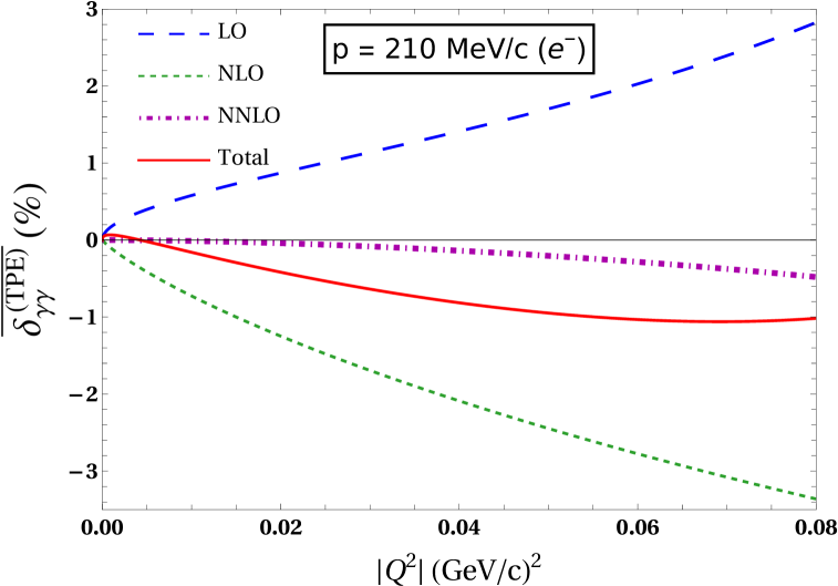
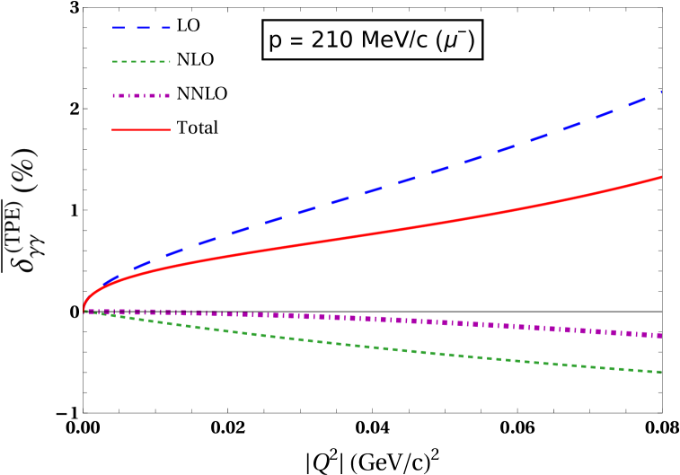
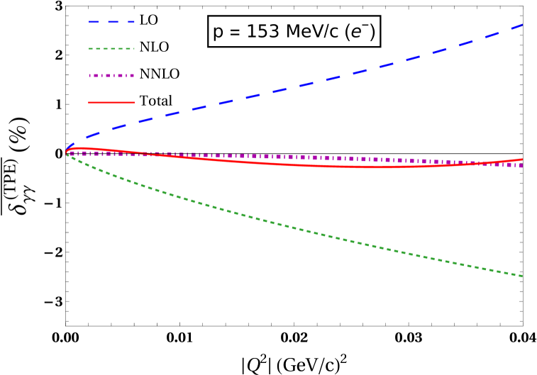
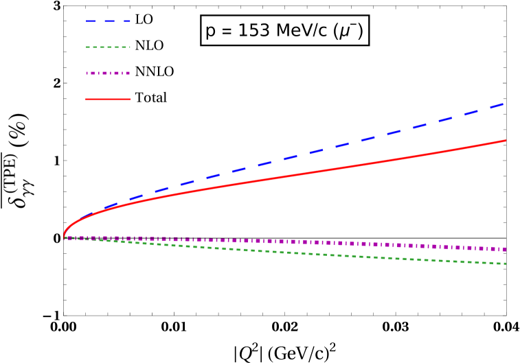
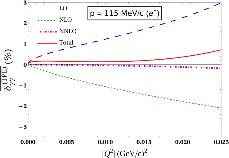
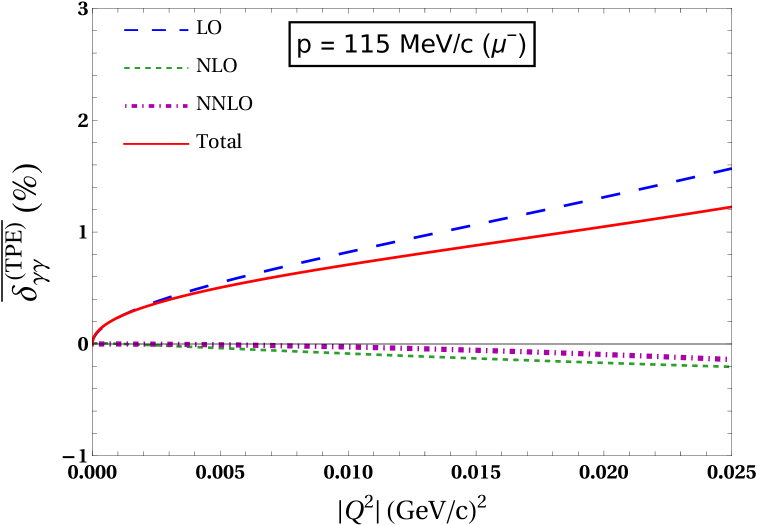
Figure 6: Comparison of the IR-finite fractional TPE contributions (invoking SPA) at various orders (LO, NLO and NNLO) in HB$\chi$PT to the e-p (left panel) and $\mu$-p (right panel) elastic scattering cross-sections as a function of the squared four-momentum transfer $|Q^{2}|$ given at the three MUSE proposed incoming lepton beam three-momenta: 210 MeV/c, 153 MeV/c, and 115 MeV/c. The LO and NLO corrections are represented by Eqs. (87) and (88), respectively. The NNLO corrections, Eqs. (89), include only the dominant proton’s form factor contribution, excluding contributions from the two-loop topologies with non-factorizable pion-loops (cf. Fig. 5). All the fractional contributions are considered relative to the LO Born differential cross-section [cf. Eq. (91)].

For the NLO TPE contributions in Eq. (88), one finds terms proportional to the so-called chiral-logarithm, $\ln{\sqrt{-\frac{Q^{2}}{2M\beta E}}}$, which are responsible for the significant negative enhancement of the electron results. This contrasts the previous SPA results of Talukdar et al. Talukdar:2019dko ; Talukdar:2020aui , where such enhancements were missing. Moreover, as already discussed in the introduction, the IR-divergence subtraction scheme used in those SPA-based works was $Q^{2}$-dependent, which contrasts with our improved $Q^{2}$-independent scheme [see Eq. (20)] (also see Ref. Choudhary:2023rsz ). Notably, modifying the TPE result of Ref. Talukdar:2019dko by incorporating the same subtraction scheme as used here, yields results similar to our NLO corrections for the electron scattering case, [see Fig. 7]. We also find that our NLO SPA results for both the electron and muon are negative, decreasing with decreasing incoming lepton-beam three-momentum. This behavior contrasts the exact NLO TPE results of Choudhary et al. Choudhary:2023rsz , where the contributions were obtained strictly positive for the muon, while for electrons they were predominantly negative for most of the low-$Q^{2}$ MUSE domain.

Regarding the NNLO corrections in Fig. 6, besides the kinematically suppressed $\mathcal{O}(1/M^{2})$ terms stemming from the LO and the NLO TPE diagrams (a)-(i), we also include the dynamical contributions from the genuine NNLO TPE amplitudes (j)-(v), some of which contain contributions from the proton’s structure. However, we find that all such structure-dependent terms, along with the NNLO seagull contribution, are kinematically suppressed to $\mathcal{O}(1/M^{3})$, and hence, dropped explicitly in the NNLO fractional TPE contributions displayed in Eqs. (83) and (84). As seen from Fig. 6, the NNLO contributions are relatively small compared to the more important LO and NLO contributions (less than $\sim 15\%$ of the NLO corrections in the MUSE regime). The negative nature of the NNLO contributions is reminiscent of the typical corrections induced by incorporating phenomenological form factors, which are known to suppress the magnitude of the overall TPE and other radiative corrections. Their magnitude increases with increasing incoming lepton momentum both for the electron and muon. Also apparent in the figure is that our NNLO results compared to the NLO are much less sensitive to the lepton mass $m_{l}$ variation.

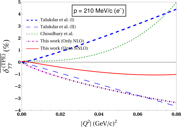
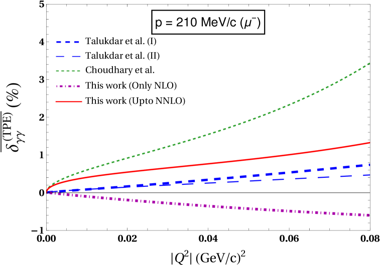
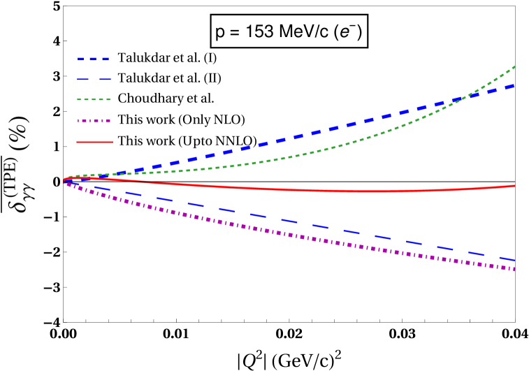
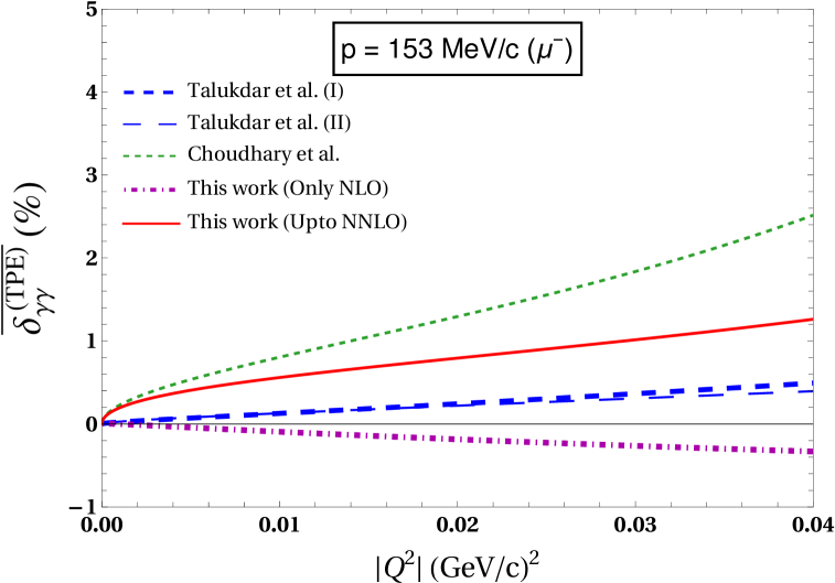
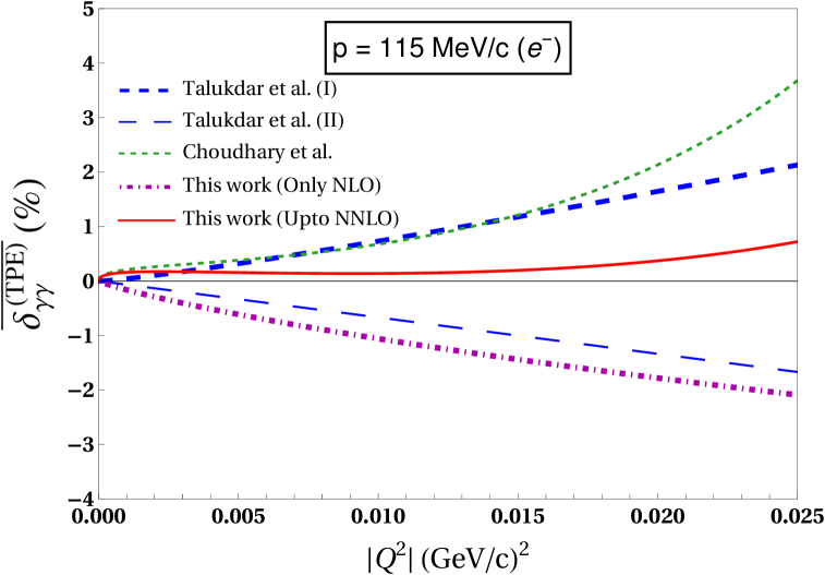
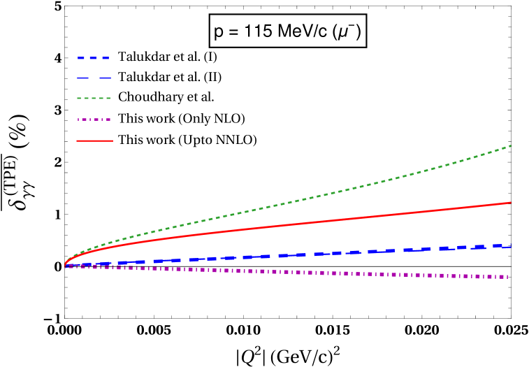
Figure 7: Comparison of our complete SPA results up to NNLO for the IR-finite TPE contributions with the analogous SPA-based NLO HB$\chi$PT calculation of Talukdar et al. Talukdar:2019dko where the LO contributions were found to vanish completely, i.e., without Feshbach-like term. Two types of plots for Talukdar et al. Talukdar:2019dko are displayed: plot (I) represents the original results of Ref. Talukdar:2019dko , while plot (II) represents modifications we made in the original expression to match the IR-subtraction scheme adopted in this work. In addition, the comparison is also shown with the exact analytical TPE evaluation in HB$\chi$PT in the work of Choudhary et al. Choudhary:2023rsz . The e-p ($\mu$-p) elastic scattering results are displayed on the left (right) panel as a function of the squared four-momentum transfer $|Q^{2}|$ at the three MUSE proposed incoming lepton beam three-momenta, 210 MeV/c, 153 MeV/c, and 115 MeV/c. The fractional contributions are considered relative to the LO Born differential cross-section [cf. Eq. (91)].

Next in Fig. 7, we display a comparison between our SPA-based TPE results with the analogous HB$\chi$PT results evaluated earlier by Talukdar et al. Talukdar:2019dko , and with the exact TPE results of Choudhary et al. Choudhary:2023rsz . The blue thick dashed curves, labeled “Talukdar et al. (I)”, represent the results of Talukdar et al. with a $Q^{2}$-dependent IR cancellation scheme which differs from the $Q^{2}$-independent scheme used in this work. The blue thin long-dashed curves, labeled “Talukdar et al. (II)”, represent the results of Talukdar et al. which we have modified by incorporating the same IR-subtraction scheme used by Choudhary et al., and also adopted in this work. Also displayed in Fig. 7 are our NLO TPE corrections to the elastic cross-section which include all $\mathcal{O}(1/M)$ terms represented by the violet dot-dashed curves labeled “This work (Only NLO)”. This, in particular, facilitates a direct comparison with our modified “Talukdar et al. (II)” results of Ref. Talukdar:2019dko , which rely on the same $Q^{2}$-independent IR-subtraction scheme while excluding the Feshbach-like term, Eq. (18). Finally, our SPA results for the total fractional TPE contributions including the partial NNLO corrections (i.e., LO+NLO+NNLO) are displayed in the figure, as represented by the red solid-line curves, labeled “This work (Upto NNLO)”. We find that our SPA results differ significantly from the corresponding exact TPE results of Choudhary et al.. Choudhary:2023rsz . Notably, in the case of NLO results for electron scattering, both our SPA and the exact TPE results of Choudhary et al. yield negative contributions at the low-$|Q^{2}|$ MUSE kinematics, with the latter NLO results being much more non-linear. In contrast, for muon scattering, our SPA versus the exact TPE evaluations yield negative versus positive NLO contributions, with the magnitudes of the SPA results smaller than the exact ones. The following comments highlight the crucial differences between our SPA and the exact TPE results of Choudhary et al. Choudhary:2023rsz , which justify the complementary features of each TPE analysis:

• Choudhary et al. features HB$\chi$PT calculations up-to-and-including NLO where it is found that the NLO corrections are numerically almost as large as the LO for electron scattering at low-$|Q^{2}|$ values. This naturally raises concerns regarding the magnitude of the NNLO corrections for the validity of the EFT convergence, which was not addressed in that work. In this regard, by extending to the dominant class of NNLO corrections which are found substantially smaller than the NLO, our SPA results validate the perturbative convergence of the HB$\chi$PT analysis employed in both works, albeit the numerical differences in the respective findings.

• Within our version of a one-loop approximation for the genuine NNLO diagrams contributing to the TPE, we include the dominant contribution from pion-loops renormalizing the proton-photon vertices, which can, in principle, bring about proton’s structure-dependent (form factors or charge radius) modifications to the TPE loops [although in our case such ${\mathcal{O}}(1/M^{2})$ terms cancel out exactly, with residual kinematically suppressed ${\mathcal{O}}(1/M^{3})$ terms neglected, cf. Eq. (81)]. This indicates that the negative NNLO TPE contributions could suppress the overall magnitude of the TPE corrections obtained in the work of Choudhary et al.

• A detailed investigation reveals that our SPA-based analysis misses the contributions from loop-integrations, such as $I(Q|1,1,1,0)$, $I(Q|1,1,0,1)$, $I^{-}(p,0|1,1,1,1)$ and $I^{+}(p^{\prime},0|1,1,1,1)$, which are present in the exact TPE analysis of Choudhary et al Choudhary:2023rsz .

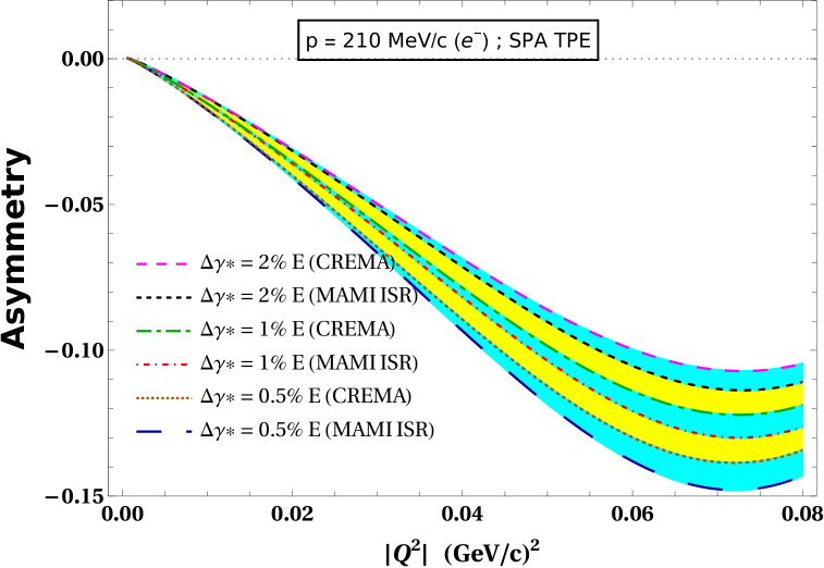
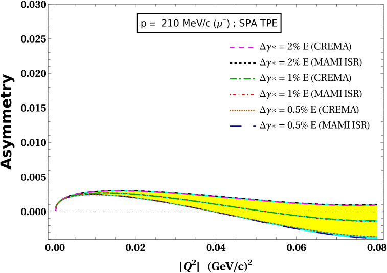
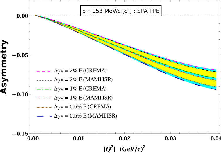
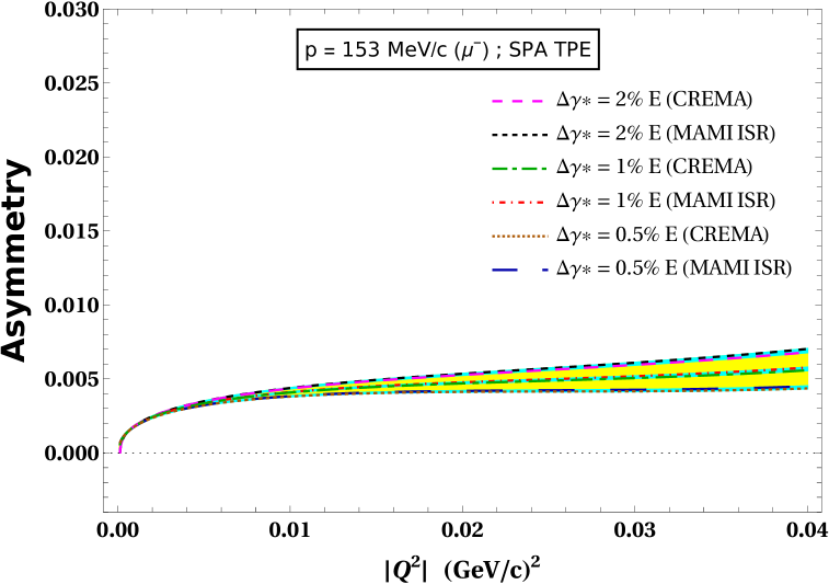
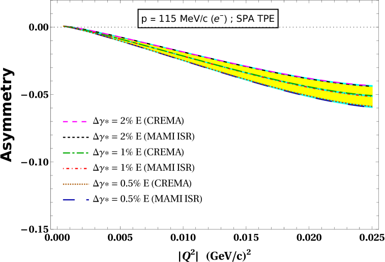
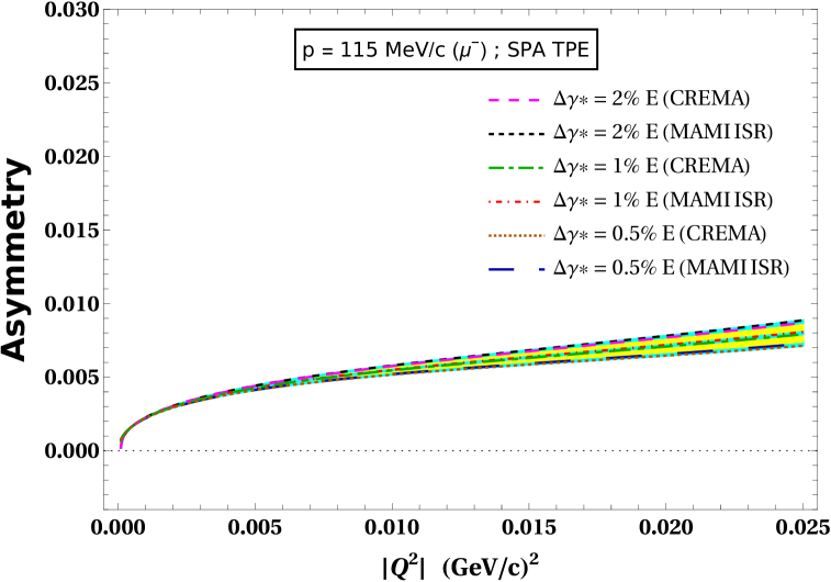
Figure 8: Our results for the charge asymmetry (${\mathcal{A}}^{(1)}_{\ell^{\pm}}$) between lepton-proton ($\ell^{-}$-p) and anti-lepton-proton ($\ell^{+}$-p) scattering cross-sections up-to-and-including NLO accuracy in HB$\chi$PT, where our SPA-based TPE contributions (LO and NLO) are taken as the input. The e-p ($\mu$-p) elastic scattering results are displayed on the left (right) panel as a function of the squared four-momentum transfer $|Q^{2}|$ at the three MUSE proposed incoming lepton beam three-momenta: 210 MeV/c, 153 MeV/c, and 115 MeV/c. The yellow bands depict the uncertainty in our predictions owing to the variation of the detector threshold, namely, $0.5\%<\Delta_{\gamma^{*}}<2\%$ of the incoming lepton energy $E$ stemming from the soft-photon bremsstrahlung contributions. Likewise, the cyan bands depict the uncertainty due to the variation of the proton’s rms charge radius within the range of the extracted values from the recent precision e-p scattering measurements by the A1 Collaboration Mihovilovic:2019jiz , and that from the erstwhile high-precision muonic hydrogen atomic-spectroscopy measurements by the CREMA Collaboration Antognini:2013txn ; Pohl:2013yb .

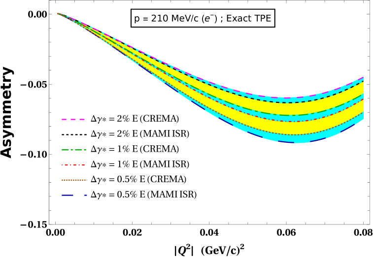
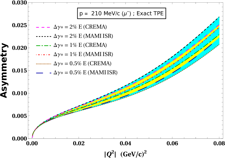
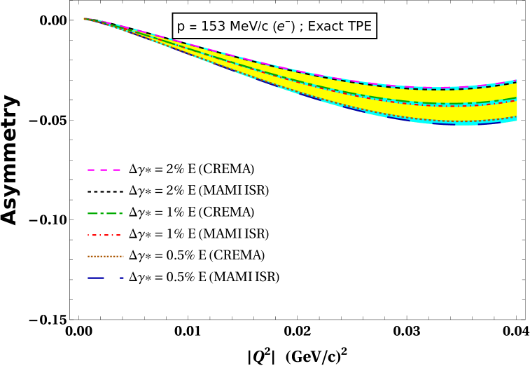
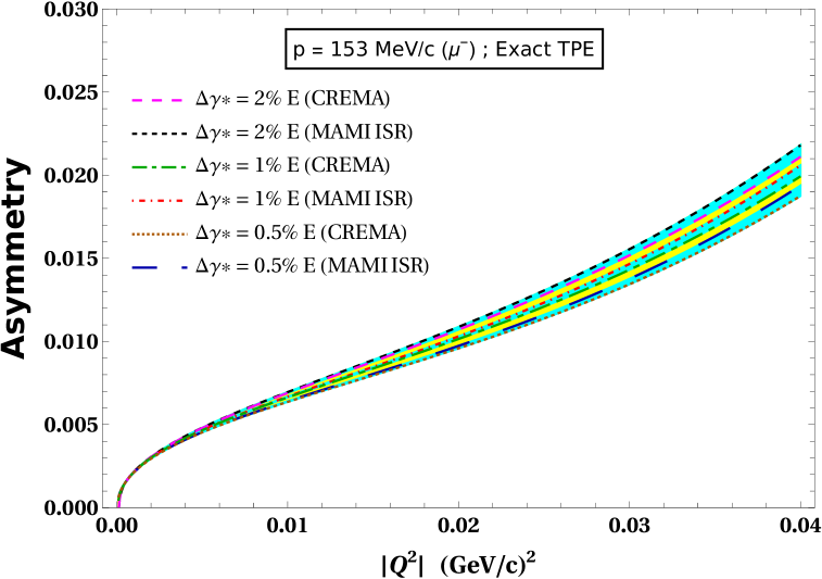
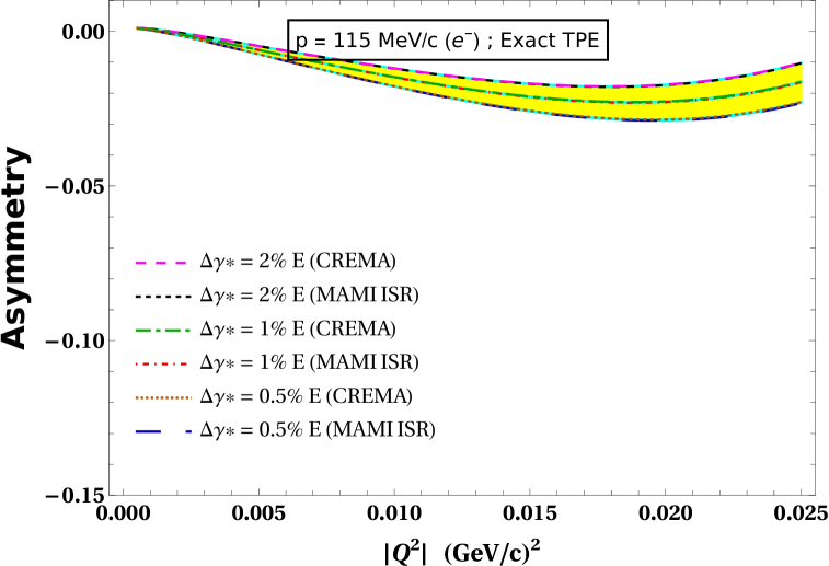
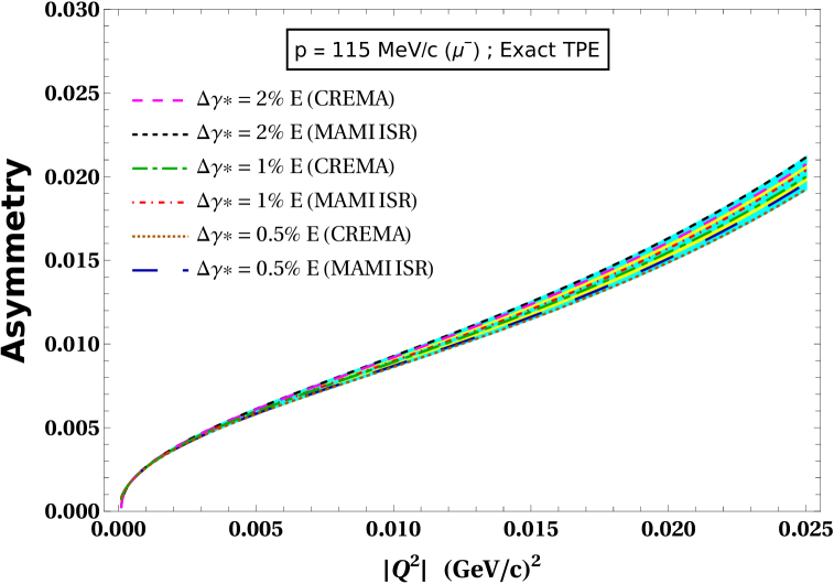
Figure 9: Our results for the charge asymmetry (${\mathcal{A}}^{(1)}_{\ell^{\pm}}$) between lepton-proton ($\ell^{-}$-p) and anti-lepton-proton ($\ell^{+}$-p) scattering cross-sections up-to-and-including NLO accuracy in HB$\chi$PT, using the exact TPE results of Choudhary et al. Choudhary:2023rsz . The e-p ($\mu$-p) elastic scattering results are displayed on the left (right) panel as a function of the squared four-momentum transfer $|Q^{2}|$ at the three MUSE proposed incoming lepton beam three-momenta: 210 MeV/c, 153 MeV/c, and 115 MeV/c. The yellow bands depict the uncertainty in our predictions owing to the variation of the detector threshold, namely, $0.5\%<\Delta_{\gamma^{*}}<2\%$ of the incoming lepton energy $E$ stemming from the soft-photon bremsstrahlung contributions. Likewise, the cyan bands depict the uncertainty due to the variation of the proton’s rms charge radius within the range of the extracted values from the recent precision e-p scattering measurements by the A1 Collaboration Mihovilovic:2019jiz , and that from the erstwhile high-precision muonic hydrogen atomic-spectroscopy measurements by the CREMA Collaboration Antognini:2013txn ; Pohl:2013yb .

We briefly comment on the theoretical error estimate for our SPA-based TPE prediction. As evident from the LO, NLO, and NNLO contributions, Eqs. (87), (88) and (89), respectively, our analytical expressions do not contain arbitrary free parameters. Therefore, the only uncertainty stems from the perturbative truncation at NNLO in the HB$\chi$PT power counting. In this work, we considered only a seemingly dominant class of NNLO contributions to the TPE at ”one-loop” approximation. The exclusion of the non-factorizable two-loop NNLO contributions, Fig. 5, leads to uncertainties that scale as the same order as the NNLO contributions themselves. We, therefore, envisage a maximum uncertainty in our TPE results of about $\sim 0.6\%$ of the LO Born differential cross-section, Eq. (91), for both lepton flavors, as revealed easily by glancing at the results of Fig. 6.

Finally, we present in Figs. 8 and  9, our numerical estimation of the charge asymmetry between lepton- and anti-lepton-proton scattering, Eq. (99), at the level of NLO accuracy, with our TPE results evaluated using SPA, and with the exactly evaluated TPE by Choudhary et al. Choudhary:2023rsz . Both the TPE and the charge-odd bremsstrahlung corrections contribute to the total charge-odd radiative corrections $\delta_{\rm odd}$, whereas the charge-even radiative and hadronic corrections to the lepton-proton OPE scattering process contribute to the total charge-even corrections $\delta_{\rm even}$. In particular, we only consider the leading hadronic corrections to the OPE $\delta^{(2)}_{\chi}$, which are NNLO in the chiral power counting.

As we previously discussed, the soft-photon bremsstrahlung corrections are an integral part of charge asymmetry results. The estimation involves the arbitrary “energy” parameter $\Delta_{\gamma^{*}}$, which serves to distinguish between the soft and hard photons Mo:1968cg . The numerical value of this parameter is identified with the resolution of the detector, which is determined based on the specifics of the experimental setup. Apart from $\Delta_{\gamma^{*}}$, the only other free parameter in our analysis is the proton’s rms electric charge radius $r_{p}$ which contributes to the hadronic chiral correction Eq. (98). To assess the sensitivity of our asymmetry results to these two free parameters, in Figs. 8 and  9, we varied $\Delta_{\gamma^{*}}$ within the range $0.5\%<\Delta_{\gamma^{*}}<2\%$ of lepton energy $E$. The radius $r_{p}$ is likewise varied within a range corresponding to the extracted value, $0.87\pm(0.014)_{\rm stat.}\pm(0.024)_{\rm syst.}\pm(0.003)_{\rm mod.}$ fm, from the recent precision e-p scattering measurements by the A1 Collaboration (MAMI) Mihovilovic:2019jiz , and the value $0.84087(39)$ fm, from the erstwhile high-precision muonic hydrogen spectroscopic measurements by the CREMA Collaboration (PSI) Antognini:2013txn ; Pohl:2013yb . The latter range serves as a rough indicator to gauge the impact of the current status of the proton’s radius discrepancy in our asymmetry estimates.

A comparison between Figs. 8 (TPE using SPA) and  9 (exact TPE) reflects that the asymmetry results are more sensitive to the above parameters for the electrons with the constituent TPE evaluated in SPA. Furthermore, we find that there is an increasing sensitivity due to the variation of the parameters with increasing $|Q^{2}|$ values and lepton beam momentum, for both electron and muon scattering cases. We find that the sensitivities due to the variations of $\Delta_{\gamma^{*}}$ and $r_{p}$ are quite contrasting for muon scattering when comparing the SPA versus exact TPE results. We also find that when comparing Figs. 8 and  9 for electron scattering, the asymmetry is more negative in the former, although in both cases their magnitudes increase with rising incoming electron momentum (notice the same ordinate scale used to compare both figures in regard to the individual leptons). In contrast, for muon scattering, the asymmetry remains predominantly positive in both SPA and exact TPE input cases, with their magnitudes slowly decreasing (increasing) in the former (latter) with rising incoming muon momentum. There is, however, one exception, namely, with the SPA-based TPE input for the muon scattering corresponding to the largest beam momentum, where the asymmetry behavior is found to be quite unusual (upper right panel in Fig. 8). In this case, the asymmetry is positive for small-$|Q^{2}|$ values, exhibiting a positive maximum with increasing $|Q^{2}|$, but then decreasing to become mostly negative in the large-$|Q^{2}|$ region for MUSE kinematics. In contrast, with the exact TPE input, the asymmetry increases dramatically with increasing incoming muon beam momentum, as seen in Fig. 9. It is worth mentioning that regarding the overall sensitivity due to $r_{p}$, we find up to 4% uncertainty with the exact TPE input results for both electron and muon scatterings at the largest values of the MUSE beam momenta.

In conclusion, we find that the SPA-based TPE evaluation yields the results (presented in this paper) are significantly different from the exact TPE results of Choudhary et al. Choudhary:2023rsz . Invoking SPA, with one or the other photon propagator in the TPE box- and cross-box diagrams set on-shell, the assumption turns out to be rather restrictive. In effect, this means that for a SPA-based evaluation which, for instance, neglects the contribution from the kinematic region with two exchanged hard-photons within the TPE loops, a significant systematic uncertainty can be introduced. Consequently, one should avoid the SPA methodology altogether to obtain reasonably precise estimates of the TPE or observables that rely on the TPE. Regarding the charge asymmetry, we have made only a preliminary estimate in this work. In the near future, we hope to improve upon our presented asymmetry results for both the electron and muon scatterings, removing further sources of systematic theoretical uncertainties. To that end, two important future directions of the present work are conceivable: (i) an improved treatment of the exact TPE results of Choudhary et al. Choudhary:2023rsz by including NNLO corrections, and (ii) inclusion of hard bremsstrahlung photons to assess the charge asymmetry, thereby removing the dependence on the arbitrary $\Delta_{\gamma^{*}}$ parameter. Currently, work is in progress in both these directions Bhoomika24 .

Appendix A Loop-integrations

In this appendix, we collect the Feynman loop-integrations employed in our analytical evaluations of the TPE diagrams, where we denote the external lepton four-momenta as $p$ and $p^{\prime}$, such that the four-momentum transfer is $Q=p-p^{\prime}$, while the loop four-momentum is denoted by $k$. These are given by the following generic scaler and tensor integrals with indices $n_{1,2,3,4}\in{\mathbb{Z}}$ and a real-valued parameter $\omega$:

$$I^{-}(p,\omega|n_{1},n_{2},n_{3},n_{4})\!\! = \!\!\frac{1}{i}\int\frac{{\rm d}^{4}k}{(2\pi)^{4}}\frac{1}{(k^{2}+i0)^{n_{1}}[(k-Q)^{2}+i0]^{n_{2}}(k^{2}-2k\cdot p+i0)^{n_{3}}(v\cdot k+\omega+i0)^{n_{4}}}\,,$$ (100)

$$I^{+}(p^{\prime},\omega|n_{1},n_{2},n_{3},n_{4})\!\! = \!\!\frac{1}{i}\int\frac{{\rm d}^{4}k}{(2\pi)^{4}}\frac{1}{(k^{2}+i0)^{n_{1}}[(k-Q)^{2}+i0]^{n_{2}}(k^{2}+2k\cdot p^{\prime}+i0)^{n_{3}}(v\cdot k+\omega+i0)^{n_{4}}}\,,$$ (101)

and

$$I^{-\mu}(p,\omega|n_{1},n_{2},n_{3},n_{4})\!\! = \!\!\frac{1}{i}\int\frac{{\rm d}^{4}k}{(2\pi)^{4}}\frac{k^{\mu}}{(k^{2}+i0)^{n_{1}}[(k-Q)^{2}+i0]^{n_{2}}(k^{2}-2k\cdot p+i0)^{n_{3}}(v\cdot k+\omega+i0)^{n_{4}}}\,,$$ (102)

respectively. The specific integrals that were used for our calculations have $\omega=0$. First, we consider the two IR-divergent loop-integrals, namely,

$$I^{-}(p,0|1,0,1,1)\!\! \equiv \!\!I^{(0)}(p,0|1,0,1,1)=\frac{1}{i}\int\frac{{\rm d}^{4}k}{(2\pi)^{4}}\frac{1}{(k^{2}+i0)\,(k^{2}-2k\cdot p+i0)\,(v\cdot k+i0)}$$ (103)

$$= \!\!-\,\frac{1}{(4\pi)^{2}\beta E}\Bigg{[}\left\{\frac{1}{\epsilon}-\gamma_{E}+\ln{\left(\frac{4\pi\mu^{2}}{m_{l}^{2}}\right)}\right\}\ln{\sqrt{\frac{1+\beta}{1-\beta}}}-{\rm Li}_{2}\left(\frac{2\beta}{1+\beta}\right)-\ln^{2}{\sqrt{\frac{1+\beta}{1-\beta}}}$$

$$\hskip 49.79231pt-\,i\pi\left\{\frac{1}{\epsilon}-\gamma_{E}+\ln{\left(\frac{4\pi\mu^{2}}{m_{l}^{2}}\right)}\right\}\Bigg{]}\,,\quad\text{and}$$

$$I^{+}(p^{\prime},0|1,0,1,1)\!\! = \!\!\frac{1}{i}\int\frac{{\rm d}^{4}k}{(2\pi)^{4}}\frac{1}{(k^{2}+i0)\,(k^{2}+2k\cdot p^{\prime}+i0)\,(v\cdot k+i0)}$$ (104)

$$= \!\!\frac{1}{(4\pi)^{2}\beta^{\prime}E^{\prime}}\Bigg{[}\left\{\frac{1}{\epsilon}-\gamma_{E}+\ln{\left(\frac{4\pi\mu^{2}}{m_{l}^{2}}\right)}\right\}\ln{\sqrt{\frac{1+\beta^{\prime}}{1-\beta^{\prime}}}}-{\rm Li}_{2}\left(\frac{2\beta^{\prime}}{1+\beta^{\prime}}\right)-\ln^{2}{\sqrt{\frac{1+\beta^{\prime}}{1-\beta^{\prime}}}}$$

$$\hskip 49.79231pt-\,i\pi\left\{\frac{1}{\epsilon}-\gamma_{E}+\ln{\left(\frac{4\pi\mu^{2}}{m_{l}^{2}}\right)}\right\}\Bigg{]}$$

$$\equiv \!\!-\,I^{(0)}(p,0|1,0,1,1)+\delta^{(1/M)}I^{+}(p^{\prime},0|1,0,1,1)+\delta^{(1/M^{2})}I^{+}(p^{\prime},0|1,0,1,1)+\mathcal{O}\left(\frac{1}{M^{3}}\right)\,,$$

where in isolating the IR-divergent parts of integrals we utilize dimensional regularization by analytically continuing the integrals to $D$-dimensional ($D=4-2\epsilon$) space-time, where the pole $\epsilon<0$ yields the IR-divergence. For convenience, we split $I^{+}(p^{\prime},0|1,0,1,1)$ into the LO [i.e., $\mathcal{O}\left(1/{M^{0}}\right)$], NLO [i.e., $\mathcal{O}\left(1/M\right)$], and NNLO [i.e., $\mathcal{O}\left(1/M^{2}\right)$] parts, thereby yielding the following expressions:

$$\delta^{(1/M)}I^{+}(p^{\prime},0|1,0,1,1)\!\! = \!\!-\,\frac{Q^{2}}{2(4\pi)^{2}ME^{2}\beta^{3}}\Bigg{[}\left\{\frac{1}{\epsilon}-\gamma_{E}+\ln{\left(\frac{4\pi\mu^{2}}{m_{l}^{2}}\right)}\right\}\left(\ln{\sqrt{\frac{1+\beta}{1-\beta}}}-\beta\right)-{\rm Li}_{2}\left(\frac{2\beta}{1+\beta}\right)$$ (105)

$$\hskip 73.97733pt-\,\ln^{2}{\sqrt{\frac{1+\beta}{1-\beta}}}+2\ln{\sqrt{\frac{1+\beta}{1-\beta}}}-i\pi\left\{\frac{1}{\epsilon}-\gamma_{E}+\ln{\left(\frac{4\pi\mu^{2}}{m_{l}^{2}}\right)}\right\}\,\,\Bigg{]}\,,$$

and

$$\delta^{(1/M^{2})}I^{+}(p^{\prime},0|1,0,1,1)\!\! = \!\!\frac{Q^{4}}{8(4\pi)^{2}M^{2}E^{3}\beta^{5}}\Bigg{[}\left\{\frac{1}{\epsilon}-\gamma_{E}+\ln{\left(\frac{4\pi\mu^{2}}{m_{l}^{2}}\right)}\right\}\left((3-\beta^{2})\ln{\sqrt{\frac{1+\beta}{1-\beta}}}-3\beta\right)-2\beta$$ (106)

$$\hskip 73.97733pt-\,(3-\beta^{2}){\rm Li}_{2}\left(\frac{2\beta}{1+\beta}\right)-(3-\beta^{2})\ln^{2}{\sqrt{\frac{1+\beta}{1-\beta}}}-2(\beta^{2}-4)$$

$$\hskip 73.97733pt\times\,\ln{\sqrt{\frac{1+\beta}{1-\beta}}}-i\pi(3-\beta^{2})\left\{\frac{1}{\epsilon}-\gamma_{E}+\ln{\left(\frac{4\pi\mu^{2}}{m_{l}^{2}}\right)}\right\}\Bigg{]}\,.$$

Here, $\beta=|{\bf p}\,|/E$ and $\beta^{\prime}=|{{\bf p}^{\prime}}\,|/E^{\prime}$ are the velocities of the incoming and outgoing lepton, respectively, and

$${\rm Li}_{2}(z)=-\int_{0}^{z}{\rm d}t\,\frac{\ln(1-t)}{t}\,,\quad\forall z\in{\mathbb{C}}\,,$$ (107)

is the standard di-logarithm (or Spence) function. The rest of the loop-integrals appearing in our TPE results are IR-finite. Splitting them into LO, NLO, and NNLO parts, they are respectively given by

$$I^{-}(p,0|0,1,1,1)\!\! = \!\!\frac{1}{i}\int\frac{{\rm d}^{4}k}{(2\pi)^{4}}\frac{1}{[(k-Q)^{2}+i0]\,(k^{2}-2k\cdot p+i0)\,(v\cdot k+i0)}$$ (108)

$$\equiv \!\!I^{(0)}(p,0|0,1,1,1)+\delta^{(1/M)}I^{-}(p,0|0,1,1,1)+\delta^{(1/M^{2})}I^{-}(p,0|0,1,1,1)+\mathcal{O}\left(\frac{1}{M^{3}}\right)\,,$$

where,

$$I^{(0)}(p,0|0,1,1,1)\!\! = \!\!-\frac{1}{(4\pi)^{2}\beta E}\Bigg{[}\frac{\pi^{2}}{6}-{\rm Li}_{2}\left(\frac{2\beta}{1+\beta}\right)-{\rm Li}_{2}\left(\frac{1+\beta}{1-\beta}\right)-2\ln^{2}{\sqrt{\frac{1+\beta}{1-\beta}}}$$ (109)

$$\hskip 51.21504pt+\,2\ln\left({-\frac{Q^{2}}{2ME\beta}}\right)\ln{\sqrt{\frac{1+\beta}{1-\beta}}}\,\,\Bigg{]}\,,$$

$$\delta^{(1/M)}I^{-}(p,0|0,1,1,1)\!\! = \!\!-\frac{Q^{2}}{(4\pi)^{2}M\beta^{3}E^{2}}\Bigg{[}-\frac{\pi^{2}}{12}-\beta+\frac{1}{2}{\rm Li}_{2}\left(\frac{2\beta}{1+\beta}\right)+\frac{1}{2}{\rm Li}_{2}\left(\frac{1+\beta}{1-\beta}\right)-(1+\beta)\ln{\sqrt{\frac{1+\beta}{1-\beta}}}$$ (110)

$$\hskip 72.55461pt+\,2\beta\ln{\sqrt{\frac{2\beta}{1-\beta}}}+\ln^{2}{\sqrt{\frac{1+\beta}{1-\beta}}}-\ln{\left(-\frac{Q^{2}}{2ME\beta}\right)}\ln{\sqrt{\frac{1+\beta}{1-\beta}}}$$

$$\hskip 72.55461pt+\,\beta\ln{\left(-\frac{Q^{2}}{2ME\beta}\right)}+i\pi\beta\Bigg{]}\,,\quad\text{and}$$

$$\delta^{(1/M^{2})}I^{-}(p,0|0,1,1,1)\!\! = \!\!\frac{Q^{4}}{8(4\pi)^{2}M^{2}E^{3}\beta^{5}}\Bigg{[}5\beta+3(1+\beta)^{2}\ln{\sqrt{\frac{1+\beta}{1-\beta}}-12\beta\ln{\sqrt{\frac{2\beta}{1-\beta}}}}-12\beta\ln{\sqrt{-\frac{Q^{2}}{2ME\beta}}}$$ (111)

$$\hskip 72.55461pt-\,(3-\beta^{2})\Bigg{\{}\frac{\pi^{2}}{6}-{\rm Li}_{2}\left(\frac{2\beta}{1+\beta}\right)-{\rm Li}_{2}\left(\frac{1+\beta}{1-\beta}\right)-2\ln^{2}{\sqrt{\frac{1+\beta}{1-\beta}}}$$

$$\hskip 72.55461pt+\,2\ln{\left(-\frac{Q^{2}}{2ME\beta}\right)}\ln{\sqrt{\frac{1+\beta}{1-\beta}}}\,\Bigg{\}}-6i\pi\beta\Bigg{]}\,.$$

Similarly, we have

$$I^{+}(p^{\prime},0|0,1,1,1)\!\! = \!\!\frac{1}{i}\int\frac{{\rm d}^{4}k}{(2\pi)^{4}}\frac{1}{[(k-Q)^{2}+i0]\,(k^{2}+2k\cdot p^{\prime}+i0)\,(v\cdot k+i0)}$$ (112)

$$\equiv \!\!-\,I^{(0)}(p,0|0,1,1,1)+\delta^{(1/M)}I^{+}(p^{\prime},0|0,1,1,1)+\delta^{(1/M^{2})}I^{+}(p^{\prime},0|0,1,1,1)+\mathcal{O}\left(\frac{1}{M^{3}}\right)\,,\quad\,$$

where,

$$\delta^{(1/M)}I^{+}(p^{\prime},0|0,1,1,1)\!\! = \!\!-\frac{Q^{2}}{(4\pi)^{2}M\beta^{3}E^{2}}\left[\ln{\sqrt{\frac{1+\beta}{1-\beta}}}-\beta\right]\,,$$ (113)

$$\delta^{(1/M^{2})}I^{+}(p^{\prime},0|0,1,1,1)\!\! = \!\!\frac{Q^{4}}{8(4\pi)^{2}M^{2}E^{3}\beta^{5}}\left[(3-\beta^{2})\ln\sqrt{{\frac{1+\beta}{1-\beta}}}-3\beta\right]\,.$$ (114)

Next, we consider

$$I^{-}(p,0|0,1,1,2)\!\! = \!\!\frac{1}{i}\int\frac{{\rm d}^{4}k}{(2\pi)^{4}}\frac{1}{[(k-Q)^{2}+i0]\,(k^{2}-2k\cdot p+i0)\,(v\cdot k+i0)^{2}}$$ (115)

$$\equiv \!\!\,MI^{(0)}(p,0|0,1,1,2)+\delta^{(1/M)}I^{+}(p^{\prime},0|0,1,1,2)+\mathcal{O}\left(\frac{1}{M^{2}}\right)\,,$$

where,

$$I^{(0)}(p,0|0,1,1,2)\!\! = \!\!-\frac{4}{(4\pi)^{2}Q^{2}E\beta}\ln{\sqrt{\frac{1+\beta}{1-\beta}}}\,,$$ (116)

$$\delta^{(1/M)}I^{-}(p,0|0,1,1,2)\!\! = \!\!-\frac{3Q^{2}}{(4\pi)^{2}ME^{3}\beta^{4}}\,.$$ (117)

Similarly, we have

$$I^{+}(p^{\prime},0|0,1,1,2)\!\! = \!\!\frac{1}{i}\int\frac{{\rm d}^{4}k}{(2\pi)^{4}}\frac{1}{[(k-Q)^{2}+i0]\,(k^{2}+2k\cdot p^{\prime}+i0)\,(v\cdot k+i0)^{2}}$$ (118)

$$\equiv \!\!-MI^{(0)}(p,0|0,1,1,2)+\delta^{(M^{0})}I^{+}(p^{\prime},0|0,1,1,2)+\delta^{(1/M)}I^{+}(p^{\prime},0|0,1,1,2)+\mathcal{O}\left(\frac{1}{M^{2}}\right)\,,\quad\,$$

where,

$$\delta^{(M^{0})}I^{+}(p^{\prime},0|0,1,1,2)\!\! = \!\!-\frac{2}{(4\pi)^{2}E^{2}\beta^{3}}\bigg{[}\ln{\sqrt{\frac{1+\beta}{1-\beta}}-\beta}\bigg{]}\,,$$ (119)

$$\delta^{(1/M)}I^{+}(p^{\prime},0|0,1,1,2)\!\! = \!\!\frac{Q^{2}}{2M(4\pi)^{2}E^{3}\beta^{5}}\left(-3\beta+(3-\beta^{2})\ln\sqrt{{\frac{1+\beta}{1-\beta}}}\,\,\right)\,.$$ (120)

It is notable that the last two integrals, namely, $I^{-}(p,0|0,1,1,2)$ and $I^{+}(p^{\prime},0|0,1,1,2)$, have the leading term of ${\mathcal{O}}(M)$, and consequently we need to consider their expansions no more than ${\mathcal{O}}(M^{-1})$, as clearly suggested by the NLO and NNLO amplitudes, Eqs. (II.2) and (81). Finally, we consider the tensor loop-integration

$$I^{-\mu}_{1}(p,0|1,1,1,0)\!\! = \!\!\frac{1}{i}\int\frac{{\rm d}^{4}k}{(2\pi)^{4}}\frac{k^{\mu}}{(k^{2}+i0)[(k-Q)^{2}+i0]\,(k^{2}-2k\cdot p+i0)}$$ (121)

$$=-\,\frac{1}{4\pi^{2}Q^{2}\nu_{l}^{2}}\left[\left(p^{\mu}-\frac{1}{2}Q^{\mu}\right)\ln\sqrt{-\frac{Q^{2}}{m_{l}^{2}}}-4\pi^{2}(Q^{2}p^{\mu}-2m_{l}^{2}Q^{\mu})I(Q|1,1,1,0)\right]\,,$$

where

$$I(Q|1,1,1,0)\!\! \equiv \!\!I^{-}(p,0|1,1,1,0)=\frac{1}{i}\int\frac{{\rm d}^{4}k}{(2\pi)^{4}}\frac{1}{(k^{2}+i0)\,[(k-Q)^{2}+i0]\,(k^{2}-2k\cdot p+i0)}$$ (122)

$$\equiv \!\!I^{+}(p^{\prime},0|1,1,1,0)=\frac{1}{i}\int\frac{{\rm d}^{4}k}{(2\pi)^{4}}\frac{1}{(k^{2}+i0)\,[(k-Q)^{2}+i0]\,(k^{2}+2k\cdot p^{\prime}+i0)}$$

$$= \!\!\frac{1}{8\pi^{2}Q^{2}\nu_{l}}\left[\frac{\pi^{2}}{3}+\ln^{2}{\sqrt{\frac{\nu_{l}+1}{\nu_{l}-1}}+{\rm Li}_{2}\left(\frac{\nu_{l}-1}{\nu_{l}+1}\right)}\right]\,.$$

References

- (1) M. K. Jones et al,, Phys. Rev. Lett. 84, 1398 (2000).
- (2) C. F. Perdrisat, V. Punjabi, M. Vanderhaeghen, Prog. Part. Nucl. Phys. 59, 694 (2007).
- (3) V. Punjabi et al., Eur. Phys. J. A 51, 79 (2015).
- (4) A. J. R. Puckett, et al., Phys. Rev. Lett. 104, 242301 (2010).
- (5) R. Pohl et al., [CREMA Collaboration] Nature 466 213, 2010.
- (6) R. Pohl, R. Gilman, G. A. Miller, and K. Pachucki, Ann. Rev. Nucl. Part. Sci. 63, 175 (2013).
- (7) A. Antognini, et al., Science 339, 417 (2013).
- (8) J. C. Bernauer and R. Pohl, Scientific American 310, 32 (2014).
- (9) C. E. Carlson, Prog. Part. Nucl. Phys. 82, 59 (2015).
- (10) J. C. Bernauer, EPJ Web Conf. 234, 01001 (2020).
- (11) J. Arrington, Phys. Rev. C 68, 034325 (2003).
- (12) P. A. M. Guichon and M. Vanderhaeghen, Phys. Rev. Lett. 91, 142303 (2003).
- (13) P. G. Blunden, W. Melnitchouk and J. A. Tjon, Phys. Rev. Lett. 91, 142304 (2003).
- (14) M. P. Rekalo and E. Tomasi-Gustafsson, Nucl. Phys. A 742, 322 (2004).
- (15) P. G. Blunden, W. Melnitchouk, and J. A. Tjon, Phys. Rev. C 72, 034612 (2005).
- (16) C. E. Carlson and M. Vanderhaeghen, Ann. Rev. Nucl. Part. Sci. 57, 171 (2007).
- (17) J. Arrington, P. G. Blunden, and W. Melnitchouk, Prog. Part. Nucl. Phys. 66, 782 (2011).
- (18) H. Gao and M. Vanderhaeghen, Rev. Mod. Phys. 94, 015002, (2022).
- (19) N. Kivel and M. Vanderhaeghen, JHEP 04, 029 (2013).
- (20) I.T. Lorenz, U.-G. Meissner,H.W. Hammer and Y.B. Dong, Phys. Rev. D 91, 014023 (2015).
- (21) O. Tomalak and M. Vanderhaeghen, Phys. Rev. D 90, 013006 (2014).
- (22) O. Tomalak and M. Vanderhaeghen, Eur. Phys. J. A 51, 24 (2015).
- (23) O. Tomalak and M. Vanderhaeghen, Phys. Rev. D 93, 013023 (2016).
- (24) O. Tomalak and M. Vanderhaeghen, Eur. Phys. J. C 76, 125 (2016).
- (25) O. Tomalak, B. Pasquini, M. Vanderhaeghen, Phys. Rev. D 95, 096001 (2017).
- (26) O. Tomalak, Eur. Phys. J. C 77, 858 (2017).
- (27) O. Koshchii and A. Afanasev, Phys. Rev. D 96, 016005 (2017).
- (28) O. Tomalak and M. Vanderhaeghen, Eur. Phys. J. C 78, 514 (2018).
- (29) R. D. Bucoveanu and H. Spiesberger, Eur. Phys. J. C 55, 57 (2019).
- (30) P. Talukdar, V. C. Shastry, U. Raha and F. Myhrer, Phys. Rev. D 101, 013008 (2020).
- (31) C. Peset, A. Pineda and O. Tomalak, Prog. Part. Nucl. Phys. 121, 103901 (2021).
- (32) P. Talukdar, V. C. Shastry, U. Raha, and F. Myhrer, Phys. Rev. D 104, 053001 (2021).
- (33) N. Kaiser, Y.-H. Lin, and U.-G. Meissner, Phys. Rev. D 105, 076006 (2022).
- (34) Q. Q. Guo and H. Q. Zhou, Phys. Rev. C 106, 015203 (2022).
- (35) T. Engel, et al., Eur. Phys. J. A 59, 253 (2023).
- (36) X. H. Cao, Q. Z. Li and H. Q. Zheng, Phys. Rev. D 105, 094008 (2022).
- (37) P. Choudhary, U. Raha, F. Myhrer, and D. Chakrabarti, Eur. Phys. J. A 60, 69 (2024).
- (38) J. Gasser and H. Leutwyler, Phys. Rept. 87, 77 (1982).
- (39) E. Jenkins and A. V. Manohar, Phys. Lett. B 255, 558 (1991).
- (40) V. Bernard, N. Kaiser and U.-G. Meissner, Nucl. Phys. B 338, 315 (1992).
- (41) G. Ecker, Phys. Lett. B 336, 508 (1994).
- (42) V. Bernard, N. Kaiser and Ulf.-G. Meißner, Int. J. Mod. Phys. E 4, 193 (1995).
- (43) R. Gilman et al., [MUSE Collaboration] AIP Conf. Proc. 1563, 167 (2013).
- (44) L. W. Mo and Yung-Su Tsai. Rev. Mod. Phys. 41, 205 (1969).
- (45) L. .C. Maximon, Rev. Mod. Phys. 41, 193 (1969).
- (46) L. C. Maximon and J. A. Tjon, Phys. Rev. C 62, 054320 (2000).
- (47) M. Vanderhaeghen, et al., Phys. Rev. C 62, 025501 (2000).
- (48) N. Fettes, Ph.D Thesis titled “Pion nucleon physics in chiral perturbation theory”, Bonn University, 2000.
- (49) S. Scherer, Adv. Nucl. Phys. 27, 277 (2003).
- (50) N. Fettes, Ulf.-G. Meißner and S. Steininger, Nucl. Phys. A 640, 199 (1998). (Corrections to misprints can be found in N. Fettes, Ph.D. dissertation, Bonn University 2000, unpublished.)
- (51) V. Bernard, H. W. Fearing, T. R. Hemmert, and Ulf.-G. Meißner, Nucl. Phys. A 635, 121 (1998); Erratum: Nucl. Phys. A 642, 563 (1998).
- (52) W. A. McKinley and H. Feshbach, Phys. Rev. 74, 1759 (1948).
- (53) B. Das, R. Goswami, P. Talukdar, U. Raha and F. Myhrer, Manuscript in preparation.
- (54) M. Mihovilovič, et al., [A1 Collboration] Eur. Phys. J. A 57, 107 (2021).
- (55) A. Antognini, et al., [CREMA Collaboration] Science 339, 417 (2013).
- (56) R. Pohl, R. Gilman, G. A. Miller, and K. Pachucki, Ann. Rev. Nucl. Part. Sci. 63, 175 (2013).