\model: Boosting Mixture of LoRA Experts Fine-Tuning with a Hybrid Routing Mechanism
Abstract
Instruction-based fine-tuning of large language models (LLMs) has achieved remarkable success in various natural language processing (NLP) tasks. Parameter-efficient fine-tuning (PEFT) methods, such as Mixture of LoRA Experts (MoLE), combine the efficiency of Low-Rank Adaptation (LoRA) with the versatility of Mixture of Experts (MoE) models, demonstrating significant potential for handling multiple downstream tasks. However, the existing routing mechanisms for MoLE often involve a trade-off between computational efficiency and predictive accuracy, and they fail to fully address the diverse expert selection demands across different transformer layers. In this work, we propose \model, a hybrid routing strategy that dynamically adjusts expert selection based on the Tsallis entropy of the router’s probability distribution. This approach mitigates router uncertainty, enhances stability, and promotes more equitable expert participation, leading to faster convergence and improved model performance. Additionally, we introduce an auxiliary loss based on Tsallis entropy to further guide the model toward convergence with reduced uncertainty, thereby improving training stability and performance. Our extensive experiments on commonsense reasoning benchmarks demonstrate that \model achieves substantial performance improvements, outperforming LoRA by 9.6% and surpassing the state-of-the-art MoLE method, MoLA, by 2.3%. We also conduct a comprehensive ablation study to evaluate the contributions of \model’s key components.
1 Introduction
Instruction-based fine-tuning of large language models (Brown et al., 2020; Chowdhery et al., 2022; Touvron et al., 2023a; b) for various downstream tasks has achieved remarkable proficiency in natural language processing tasks (Chung et al., 2022; Iyer et al., 2022; Zheng et al., 2024). To significantly reduce the computational and memory resources required for full parameter fine-tuning, parameter-efficient fine-tuning methods have emerged (Houlsby et al., 2019; Li & Liang, 2021; Lester et al., 2021; Ben-Zaken et al., 2021; Liu et al., 2022). Among these, LoRA (Hu et al., 2021) has gained popularity due to its ability to reduce substantial computational costs. To maintain both cross-task generalization and computational efficiency, a promising solution (Yang et al., 2024; Luo et al., 2024; Feng et al., 2024) is to design an architecture that combines the resource-efficient features of LoRA with the versatility of Mixture of Experts (MoE) models (Wu et al., 2024a; Dou et al., 2024; Gou et al., 2023; Liu et al., 2023; Feng et al., 2024). These methods are often referred to as Mixture of LoRA Experts (MoLE). The routing mechanisms of these MoLE methods are mostly derived from standard MoE models, where a fixed number of expert networks are activated. However, recent studies indicate that the requirements for experts vary across different transformer layers (Gao et al., 2024; Zeng et al., 2024), suggesting that the routing mechanism requires further modifications to account for these factors.
Current routing mechanisms (Cai et al., 2024) can be broadly classified into two categories: 1) Soft Routing: These methods activate all expert networks for each input token, which typically leads to improvement in prediction accuracy (Ma et al., 2018; Nie et al., 2021; Wu et al., 2024c; Dou et al., 2024; Pan et al., 2024). However, this comes at the cost of significant computational overhead, as all experts are involved in the computation (Shazeer et al., 2017). 2) Sparse Routing: These approaches enhance model efficiency by activating only a subset of experts (Shazeer et al., 2017). Some techniques route each token to a single expert (Fedus et al., 2022), while others activate multiple experts, such as using Top-K (Zhou et al., 2022) or Top-P (Huang et al., 2024), or employing uncertainty-based routing (Wu et al., 2024b). Although sparse routing improves parameter efficiency, it often results in an imbalanced workload among experts, making it necessary to include an auxiliary loss functions to ensure the balance. Though both of these routing techniques aim to select the optimal set of experts for each input token, neither provides a fully comprehensive solution that accounts for the diverse and complex factors affecting model performance, which raises a key question: How can we design a hybrid routing approach that considers these factors holistically to provide a more complete solution for MoE and MoLE models?
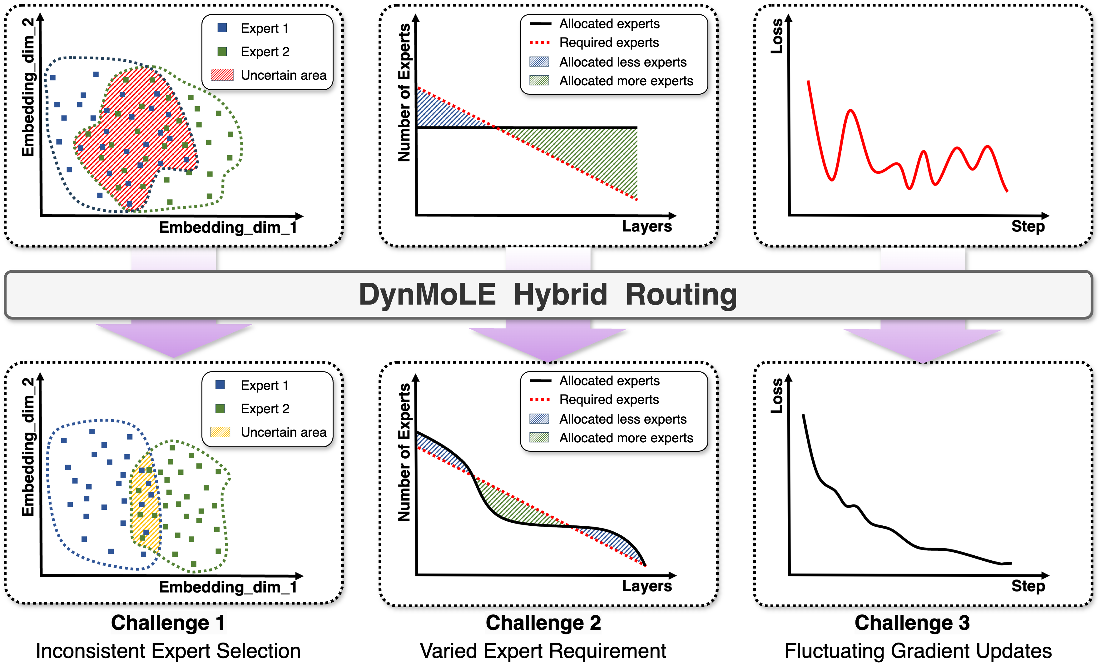
To answer this question, several critical challenges emerge: 1) Inconsistent Expert Selection occurs when flat probability distributions lead to similar inputs activating different experts, resulting in unstable expert training. 2) Varied Expert Requirements across the model, as noted by Gao et al. (2024); Zeng et al. (2024), leads to uneven expert loads when the number of activated experts is fixed across all layers. Finally, 3) Fluctuating Gradient Updates resulting from uncertain routing decisions, cause fluctuations in gradient flows, which adversely affect convergence speed and stability during model training. These challenges are illustrated in Figure 1.
To address these challenges, we propose \model (Dynamic Routing for Mixture of LoRA Experts), a hybrid routing approach designed to reduce router uncertainty in Mixture of LoRA Experts adapters for parameter-efficient fine-tuning of large language models. Our approach leverages the mathematical properties of Tsallis entropy (Tsallis, 1988), a generalized entropy measure, to develop adaptive routing strategies that effectively minimize router uncertainty. Furthermore, we introduce an auxiliary loss based on Tsallis entropy to guide the model towards convergence with reduced uncertainty, thus improving training stability and performance. By preventing over-reliance on certain experts and promoting more equitable engagement across all experts, this method fosters a diverse and robust set of expert contributions. This approach not only optimizes computational resource allocation but also enhances overall model performance by improving decision consistency and stability during training.
Summary of Contributions:
-
1.
We identify the uncertainty problem in MoE routers and theoretically derive their optimal probability distribution, which we term the Peaked Distribution. Through formal reasoning, we prove that Tsallis entropy provides a more effective quantification of routing uncertainty compared to traditional measures.
-
2.
We propose a hybrid strategy, called \model, which enables the routing mechanism to dynamically adjust based on the entropy of the routing distribution for each token, making expert selection more flexible and efficient. Additionally, we introduce an auxiliary loss for \model based on T sallis entropy, to guide the model toward convergence with reduced uncertainty, improving training stability and performance.
-
3.
We validate the effectiveness of \model using widely recognized benchmarks, as used in prior works. The results demonstrate that \model achieves remarkable performance, outperforming LoRA by 9.6% and MoLA, a state-of-the-art MoLE method, by 2.3%. Furthermore, we conducted a comprehensive ablation study to explore the effectiveness of \model’s key components.
2 Background
In this section, we introduce the background of the Mixture of Experts (MoE) and Mixture of Large Experts (MoLE), review existing popular routing strategies, and provide the mathematical definitions of uncertainty and entropy.
2.1 Mixture-of-Experts
First introduced in 1991 by Jacobs et al. (1991), the Mixture-of-Experts (MoE) architecture has seen a resurgence in the context of modern large-scale models, largely attributed to the work of Shazeer et al. (2017), Mustafa et al. (2022), Lepikhin et al. (2020), and Fedus et al. (2022). Their contributions have made MoE a promising approach for scaling models without significantly increasing computational overhead.
Each MoE layer consists of independent networks, referred to as experts, denoted by , along with a gating function , which assigns weights to each expert based on a probability distribution. The forward propagation process for a given input can be mathematically expressed as:
| (1) |
where router logits represent the routing probabilities for each expert. Each expert produces an output based on the input , allowing the MoE architecture to leverage the strengths of multiple specialized models.
In this paper, we focus exclusively on routing strategies for MoLE due to the computational resource limitations of our team. The pre-training and fine-tuning of MoE models require computational resources beyond our current capacity.
2.2 Mixture-of-LoRA-Experts
The MoLE architecture (Wu et al., 2024c) extends the traditional Mixture of Experts approach by integrating Low-Rank Adaptation into expert layers, significantly enhancing computational efficiency. In a MoLE layer, each expert is a LoRA-enhanced module that updates only a subset of parameters while leveraging the pretrained knowledge of the base model.
Low-Rank Adaptation, introduced by Hu et al. (2021), proposes a method that adjusts only a small number of additional parameters, rather than updating the entire weight matrix of the model. A LoRA block consists of two matrices, and , where and represent the dimensions of the pretrained weight matrix in large language models. The parameter is the low-rank dimension, with . The updated weights are computed as:
| (2) |
where represents the LoRA-induced weight update. Formally, given experts in a MoLE layer, denoted by , and router logits representing the routing probabilities for each expert, the forward propagation process for a given hidden state is calculated as:
| (3) |
where denotes the pretrained weights of the base model, and represents the weight updates generated by the LoRA-enhanced experts. Each expert computes its output using the LoRA update rule:
| (4) |
with and . The low-rank matrix multiplication significantly reduces the number of trainable parameters, improving memory efficiency and accelerating fine-tuning compared to standard MoE architectures. By incorporating the parameter-efficient updates of LoRA, MoLE significantly enhances both computational efficiency and model performance, especially in scenarios that require fine-tuning across multiple tasks.
2.3 Routing Algorithms
Softmax Routing
As a classic non-sparse gating function (Jordan & Jacobs, 1994), it involves multiplying the input by a trainable weight matrix and then applying the softmax function.
| (5) |
This standard routing mechanism, often referred to as soft routing, is the foundation of all MoE routing algorithms, enabling the MoE model to adaptively allocate resources based on the specific requirements of the input.
Top-K Routing
This is one of the most commonly used MoE routing algorithms. Let represent the sorted probability distribution over experts for the input token , and the algorithm is then defined as follows:
| (6) |
where is the probability assigned to expert , and is the -th highest probability in . Top-k routing selects the experts with the highest probabilities, balancing efficiency and performance.
Top-P Routing
Introduced by Huang et al. (2024), this algorithm aims to achieve variability in expert selection. It activates experts dynamically by selecting those whose cumulative probability exceeds the given threshold. This flexibility allows for tailored expert activation based on each token. The Top-p algorithm is formulated as follows:
| (7) |
where denotes the -th highest probability in the sorted probability distribution , and is the cumulative probability threshold. The algorithm selects the smallest set of experts whose cumulative probability is at least , enhancing both efficiency and adaptability.
2.4 Uncertainty and Entropy
Entropy was first introduced by Shannon (1948) to quantify the amount of ”choice” involved in the selection of an event, or the level of uncertainty in its probability distribution. The Shannon entropy is defined as:
| (8) |
where represents a probability distribution over events.
Shannon entropy has been widely applied in various fields, such as natural language processing and machine learning (Jelinek, 1980; Quinlan, 1986). However, Alomani & Kayid (2023) argues that the non-additive property of Tsallis entropy (Tsallis, 1988) provides an advantage over Shannon entropy in handling complex systems and non-Gaussian distributions. Tsallis entropy introduces a tunable parameter , which offers greater flexibility in measuring uncertainty under different conditions. The parameter , known as the entropic index, controls the degree of non-extensivity. The Tsallis entropy is defined as:
| (9) |
3 Deep Dive into the Routing Mechanism
In this section, we present an in-depth analysis of the routing mechanism employed in MoE and MoLE architectures.
3.1 What is the ideal distribution of routing weights?
Given an -expert MoE model using a soft routing algorithm, the router generates a probability distribution normalized by Softmax function. The distribution corresponds to the proportion of outputs from each expert. The initial distribution is set as uniform. It is optimized during training to minimize a loss function which is convex and differentiable. is the model’s predicted output for input , and is the true label. From A.1, we proof that the gradient of the loss function with respect to is proportional to the expert output , that is:
| (10) |
This indicates that the variation of during training is highly dependent on the contributions of the experts to the model’s output, where the expert outputs directly influence the direction and magnitude of the weight updates. In other words, for experts who contribute to a reduction in loss, the gating network increases their weights; For other experts who result in an increase in loss, it decreases their weight.
Ideally, when the model completely converges, the weights that assigned to the subset of experts who contribute most significantly to loss reduction, will be close to 1. This causes the distribution of to approach an indicative distribution, expressed in a characteristic function form as follows:
| (11) |
Though in practice, due to regularization terms and numerical stability, cannot form a perfect indicative distribution, the overall trend of allocating higher weights to a smaller subset of experts, will form a peaked distribution, as shown in Figure 3. We use uncertainty to describe how much the current distribution deviates from the ideal peaked distribution (indicative distribution). A greater uncertainty indicates a more uniform distribution and higher confusion in the router selection. However, since it is hard to define peaked distribution directly in an analytic expression mathematically, traditional measures such as KL divergence based on mutual information, are inadequate. Therefore, we introduce the concept of entropy from information theory.
3.2 Tsallis Entropy vs. Shannon Entropy
Tsallis Entropy Provide More Flexible.
As , the Tsallis entropy degenerates to the Shannon entropy:
| (12) |
The Tsallis entropy provides a continuous framework that includes the Shannon entropy as a special case. The entropic-index acts as a tunable hyperparameter, offering a powerful tool. By adjusting , we can modulate the sensitivity of the entropy to the probability distribution, making it a more adaptable and flexible tool across various scenarios. The detail information is at A.2.1
Tsallis Entropy Provide More Training Stability.
Consider a loss function that incorporates an entropy regularization term: , where is the regularization coefficient and quantifies the uncertainty in the router’s output. Now, let us compare the loss functions using Shannon entropy and Tsallis entropy, respectively. Let represent the routing probability of expert :
| (13) | ||||
| (14) |
When optimizing these loss functions via gradient descent, the gradients with respect to are given by:
| (15) | ||||
| (16) |
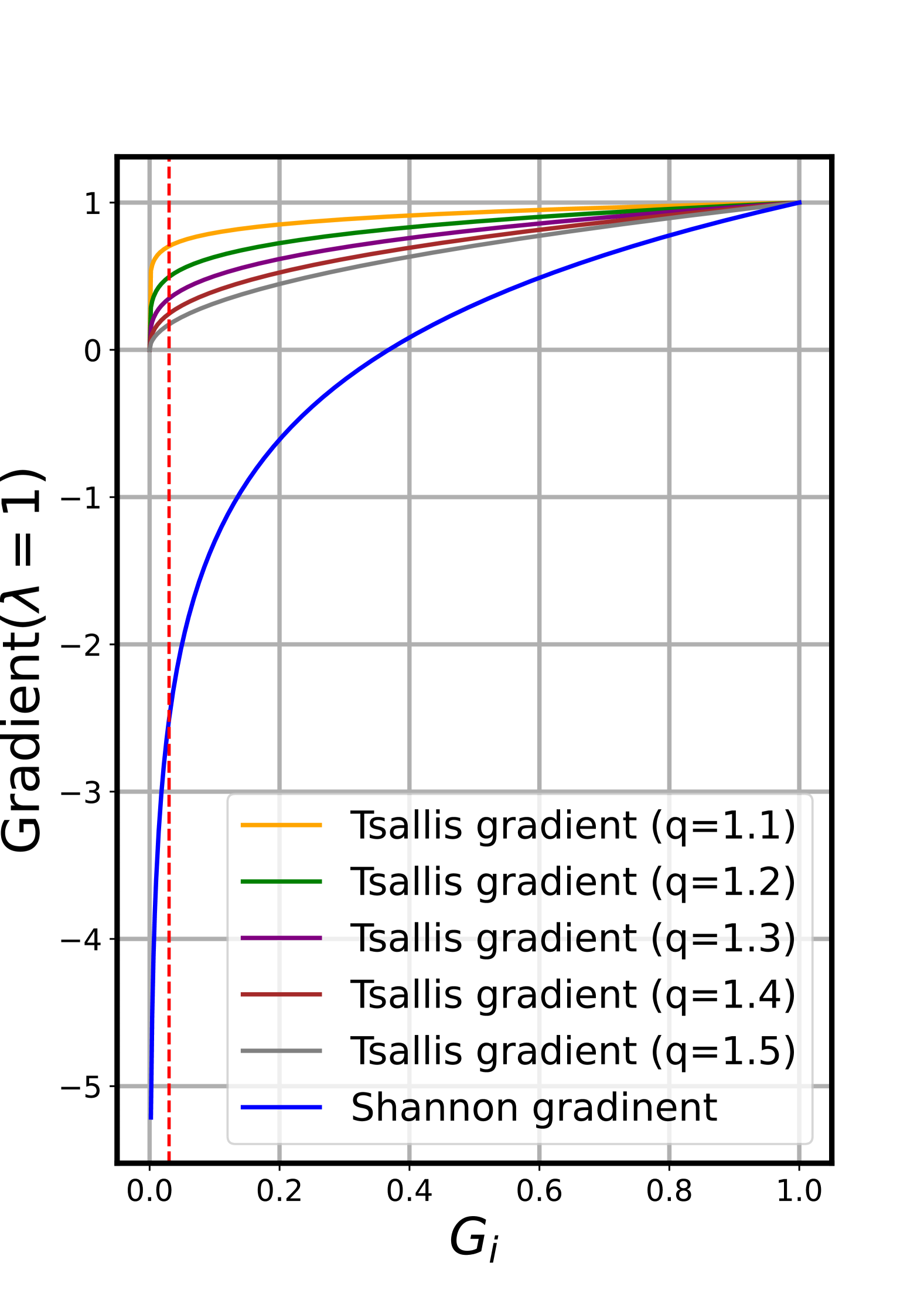
Figure 2 clearly shows the trend of gradients of the two entropy functions as changes. For Shannon entropy, as , , which can lead to steep gradient magnitudes and unstable updates. In contrast, for Tsallis entropy, as , the gradient (), reducing the impact of low-probability events and providing a more stable optimization process.
Tsallis Entropy Provide More Certainty: As increases, Tsallis entropy assigns greater weights to high-probability events in the entropy calculation, while the contribution from low-probability events diminishes. This encourages the optimization process to choose a few experts with higher probabilities. As a result, the model is biased towards reliable experts and avoids the uncertain ones, effectively reducing the overall uncertainty in the decision-making process.
4 \model
In this section, we present the routing algorithm used in \model, which integrates entropy-based selection across various routing strategies to efficiently allocate tokens to experts, as shown in Figure 3(c). This approach, termed dynamic routing, leverages Tsallis entropy to dynamically switch between soft routing, top- routing, and top- routing mechanisms. By assigning the most suitable experts to each token, we reduce routing uncertainty and improve model efficiency. Additionally, we incorporate Tsallis entropy into an auxiliary loss to guide the model towards convergence with reduced uncertainty.
4.1 Entropy-based Intelligent Hybrid Routing
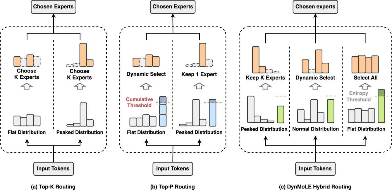
In this study, we use Tsallis entropy to capture the deviation from the ideal peaked distribution, providing greater flexibility than KL divergence. While Top-k and Top-p routing are effective, both struggle when the router has high uncertainty, leading to nearly uniform probability distributions and reducing expert prioritization, which results in suboptimal performance.
To address this, we propose \model, a hybrid strategy that dynamically adjusts routing based on the entropy of each token. For high-entropy tokens, indicating greater uncertainty, we use soft routing, allowing the model to select from a broader set of experts. For low-entropy tokens, a more deterministic Top-p routing is applied to focus on a narrower set of likely experts. Additionally, at least experts are always activated to prevent overfitting. This dynamic approach balances exploration and exploitation, improving performance across different conditions.
Given the sorted router probabilities for the input token as , and the Tsallis entropy of the router probability as , with a routing threshold , the hybrid routing can be expressed as:
| (17) |
where is defined as:
| (18) |
where represents the -th largest probability in for the Top-p selection, and denotes the -th largest probability for the Top-k selection. The function selects the Top-p fraction of probabilities, while ensures that at least experts are selected, guaranteeing sufficient diversity in expert participation based on router probabilities.
4.2 Auxiliary Entropy Loss
To further reduce the uncertainty of the router and promote balanced expert usage, we introduce an auxiliary loss based on Tsallis entropy and load balancing. Given experts, the sorted router probabilities for the input token are denoted by , with the Tsallis entropy of the router probability defined as . For a batch containing tokens, the entropy loss is computed as:
| (19) |
where is a multiplicative coefficient controlling the impact of the entropy loss.
To encourage a balanced load across experts, we also introduce a load balance loss from Fedus et al. (2022) defined as:
| (20) |
The overall auxiliary loss combines both the entropy loss and the load balance loss:
| (21) |
By incorporating this auxiliary loss, \model improves model performance by addressing both router uncertainty (through the Tsallis entropy loss) and router imbalance (through the load balance loss), leading to more efficient expert utilization and reduced uncertainty in routing decisions.
5 Experiments
| PEFT Method | RTE | ARC-e | ARC-c | BoolQ | OBQA | PIQA | SIQA | HellaS | WinoG | AVG. |
|---|---|---|---|---|---|---|---|---|---|---|
| LoRA | 52.7 | 73.8 | 50.9 | 68.2 | 77.4 | 81.1 | 69.9 | 88.4 | 68.8 | 70.1 |
| DoRA | 52.7 | 76.5 | 52.8 | 71.7 | 78.6 | 82.7 | 74.1 | 89.6 | 69.3 | 72.0 |
| LoRAMoE (Soft Routing) | 55.6 | 75.7 | 51.5 | 71.7 | 78.4 | 81.9 | 77.7 | 93.5 | 75.6 | 73.5 |
| MoLA (Top-K) | 69.3 | 76.7 | 52.4 | 72.3 | 78.2 | 82.0 | 78.7 | 93.2 | 75.1 | 75.3 |
| \model (Top-P) | 70.8 | 76.1 | 52.6 | 72.9 | 76.2 | 82.1 | 78.1 | 93.7 | 77.8 | 75.6 |
| \model(-) | 69.0 | 76.8 | 54.9 | 73.5 | 78.0 | 81.9 | 78.1 | 93.2 | 76.7 | 75.8 |
| \model | 80.1 | 78.6 | 56.0 | 72.9 | 79.2 | 82.5 | 78.5 | 92.9 | 77.8 | 77.6 |
(-) Indicates that \model trained without auxiliary entropy loss.
In this section, we present a comprehensive evaluation of \model. We compare the performance of \model with other state-of-the-art fine-tuning methods. Our experiments are designed to assess the generalization capability of \model in handling diverse tasks. Through extensive comparisons, we demonstrate that \model consistently outperforms baseline methods in terms of accuracy, particularly when integrated with entropy-based routing. Additionally, we show that \model achieves superior performance while maintaining parameter efficiency, highlighting its effectiveness in large language model fine-tuning.
5.1 Experimental Setup
Datasets. To evaluate the effectiveness of \model, we conducted experiments on a diverse set of commonsense reasoning datasets, following prior work (Liu et al., 2024; Li et al., 2024). The datasets are as follows: ARC(Clark et al., 2018), OpenBookQA(Mihaylov et al., 2018), PIQA(Bisk et al., 2020), SocialIQA(Sap et al., 2019), BoolQ(Clark et al., 2019), Hellaswag(Zellers et al., 2019), Winogrande(Sakaguchi et al., 2021), and GLUE(Wang, 2018). These datasets provide a comprehensive assessment of LLMs across various challenges, ranging from scientific queries to commonsense inference. The performance of all methods are measured using accuracy across all datasets. Further details are provided in Appendix A.3.
Baselines. In line with previous studies (Dou et al., 2024; Gao et al., 2024), we employed the widely-adopted Llama-2-7B as the base model. To thoroughly assess the performance of \model, we compared it against several prominent parameter-efficient fine-tuning (PEFT) methods, including LoRA(Hu et al., 2021), DoRA(Liu et al., 2024), LoRAMoE(Dou et al., 2024) (representing soft routing), and MoLA(Gao et al., 2024) (representing Top-K routing). While no existing PEFT methods explicitly use the Top-P routing strategy(Huang et al., 2024), we fixed \model’s routing algorithm to Top-P to evaluate the performance of all fundamental routing strategies.
Settings. To ensure parameter consistency across experiments, both LoRA and DoRA are initialized with a rank of , while LoRAMoE and MoLA are initialized with a rank of across 6 experts. For all baselines, we apply updates to the , , and weights within the feed-forward network (FFN) layers to ensure fair comparisons. Importantly, we control the number of trainable parameters across all methods, ensuring that \model and other MoE-based approaches have an identical number of trainable parameters—approximately 3% (200 million) of the total model parameters. Further details on hyperparameters are provided in Appendix A.4.
5.2 Main Results
Table 1 provides a comprehensive comparison of various PEFT methods, applied to the LLaMA-2-7B model across a diverse set of benchmarks. \model consistently demonstrates superior performance, especially when combined with entropy loss, achieving an average accuracy of 77.6%, which surpasses all baseline methods. These results underscore the effectiveness of incorporating Tsallis entropy as a measure to improve routing decisions in MoE-based architectures. For individual tasks, \model with entropy loss exhibits remarkable improvements in challenging benchmarks such as ARC-c and PIQA, achieving 56.0% and 82.5%, respectively. In particular, \model outperforms traditional PEFT method LoRA by 7.5% and state-of-art PEFT method DoRA by 4.6%, clearly demonstrating the superiority of the MoLE.
To further validate the efficacy of our proposed hybrid routing strategy, We included three important baselines: LoRAMoLE, MoLA, and \model (Top-p), representing soft routing, Top-k routing, and Top-p routing, respectively. The Top-p method is effectively implemented by disabling the soft routing mechanism, eliminating the entropy loss calculation of \model, and reducing the minimum number of activated experts(Refers to the super parameter Keep-Top-k) to one. LoRAMoE, as a soft MoE method, achieved an average accuracy of 73.5%. It combines the strengths of the LoRA module and the MoE architecture, leading to considerable improvements over traditional PEFT methods, yet there is still significant room for improvement in enhancing the specialization of its experts. While MoLA achieves an average accuracy of 75.3%, showcasing that although Top-k routing is competitive, it struggles to dynamically adjust the number of active experts based on token uncertainty. On the other hand, \model (Top-p) delivers a commendable performance with an average accuracy of 75.6%, but its pure Top-p routing mechanism does not fully exploit the flexibility required for dynamic token-expert assignment (Detailed results are shown in Appendix A.5).
The comparisons above highlight the advantage of \model’s hybrid routing strategy, which leverages the benefits of both Top-p and Top-k mechanisms. \model(-) leverages Tsallis entropy to assist the router in customizing token routing, surpassing other advanced MoLE methods by more than 0.2%. Notably, by integrating a newly designed auxiliary entropy loss, \model optimizes both of the router uncertainty and load balancing among experts more effectively, maintaining an accuracy advantage of over 2% compared to other MoLE methods. In particular, in benchmarks like ARC-c and OBQA, the performance gap is narrower, yet \model still maintains a consistent lead. This consistent performance across tasks highlights \model’s strong generalization ability, even in scenarios where the distinction between models is less pronounced.
5.3 Ablation Studies
In this section, we present a comprehensive ablation study to analyze the impact of various key hyperparameters on the performance of \model, across the ARC, OpenBookQA, BoolQ, and PIQA datasets using LLaMA-2-7B. The results of these ablations, summarized in Figure 4.

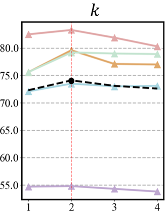
5.3.1 Impact of Different Entropy Settings on \model’s Performance
In this part, we primarily discuss the impact of three entropy-related factors on model performance:
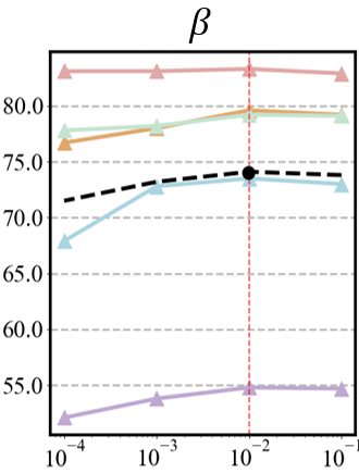
Entropy Loss Coefficient refers to a key parameter that balances the proportions of Tsallis entropy loss and load balance loss (Equation 19). We designed different values ranging from to . Figure 4(a) shows that our findings indicated an entropy router loss coefficient of achieved the highest average accuracy, effectively addressing the challenges of imbalanced expert selection. Conversely, disabling the entropy router loss or employing excessively high coefficients disrupts the balance between the two losses, leading to suboptimal performance.
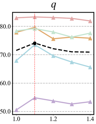
Entropic Index is the parameter in Tsallis entropy (Equation 9), which controls the degree of non-extensivity in the system. It adjusts how much weight is given to rare versus frequent events in the routing mechanism. When , Tsallis entropy reverts to Shannon entropy, treating all token-routing decisions uniformly. However, varying allows the model to emphasize or de-emphasize token assignments to experts based on their likelihood, influencing the balance between exploration (specialization of experts) and exploitation (generalization). We conducted experiments by selecting the entropic index within the range of 1.0 to 1.4 and find that an entropic index of 1.1 yielded the best overall performance(Figure 4(b)), suggesting that introducing Tsallis entropy rather than Shannon entropy allows for better adaptation to task complexity. Deviating from this optimal value, either by increasing or decreasing , led to reduced accuracy. This indicates the critical role of in fine-tuning the routing strategy and balancing expert specialization with generalization.
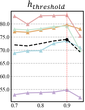
Entropy Threshold defines the soft routing threshold in \model. Typically, tokens with higher entropy lead to unclear routing decisions. In our method, we send high-entropy tokens to all experts through soft routing, allowing them to participate in the gradient update. Therefore, setting a reasonable threshold to constrain the soft routing algorithm is crucial. We collect the performance data for models with the entropy threshold set from 0.7 to 0.95, and find that an entropy threshold of 0.9 produced the highest accuracy (Figure 4(c)). Lower thresholds led to the over-selection of experts, causing computational inefficiency without significant performance gains, while higher thresholds resulted in under-utilization of experts, limiting the model’s capacity.
5.3.2 Identifying the Optimal Hyperparameter for Effective Expert Selection
This part include the discussion on two hyperparameters that closely related to expert selection.
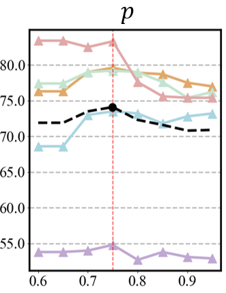
Top-p refers to the threshold in the Top-p algorithm (Huang et al., 2024), originally designed for MoE models. This algorithm collects the confidence level of each expert in handling input and activates a number of experts based on cumulative probability. We examined the impact of various values, ranging from 0.6 to 0.95, and found that a Top-p value of 0.75 resulted in the highest accuracy (Figure 4(d)). These results highlight the importance of selecting an optimal Top-p value to balance expert specialization and generalization, while also demonstrating the superior adaptability of \model compared to the Top-p approach (Figure 6).
Keep-Top-k means the minimum number of activated experts in our architecture. The work on the Switch Transformer(Fedus et al., 2022) defined expert capacity, noting that if tokens are unevenly dispatched, certain experts may overflow. Due to the limited number of activated parameters, the expert capacity of MoLE is lower than that of MoE models, and during fine-tuning, activating only one expert can lead to overfitting, therefore, we tested different values ranging from 1 to 4 on the dynamic routing strategy in \model to explore the optimal minimum number of activated experts. We find that increasing to 2 provided the necessary parameter activation, resulting in the best performance improvements (Figure 4(e)), maximally avoiding overfitting issues.
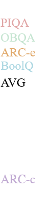
By appropriately configuring the parameters mentioned above, the experiments demonstrated a significant improvement in \model’s performance. Figure 5 shows the change in loss during fine-tuning on the GLUE-RTE dataset. We treat every 320 training steps as one round and calculate the mean and standard deviation for each round, resulting in a significantly lower average loss compared to other methods This improvement is especially evident after 12 rounds, where \model outperforms MoLA, LoRAMoE, and Top-p strategies, highlighting its effectiveness in mitigating training uncertainty. Additionally, by expanding the token allocation in three dimensions, \model shows greater ability than the Top-p method in reducing system entropy and efficiently assigning tokens to optimal experts (refer to Appendix A.6 for more details).
6 Conclusion
In this paper, we introduce \model, a hybrid routing strategy that enables the routing mechanism to dynamically adjust based on the entropy of the router’s probability distribution for each token. This dynamic adjustment allows for more flexible and efficient expert selection, optimizing performance across diverse conditions while balancing exploration and exploitation in token routing. Our extensive experiments on commonsense reasoning benchmarks demonstrate that \model achieves significant performance improvements.
References
- Alomani & Kayid (2023) Ghadah Alomani and Mohamed Kayid. Further properties of tsallis entropy and its application. Entropy, 25(2):199, 2023.
- Ben-Zaken et al. (2021) Elad Ben-Zaken, Shauli Ravfogel, and Yoav Goldberg. Bitfit: Simple parameter-efficient fine-tuning for transformer-based masked language-models. ArXiv, 2021.
- Bisk et al. (2020) Yonatan Bisk, Rowan Zellers, Jianfeng Gao, Yejin Choi, et al. Piqa: Reasoning about physical commonsense in natural language. AAAI, 2020.
- Brown et al. (2020) Tom B. Brown, Benjamin Mann, Nick Ryder, Melanie Subbiah, Jared Kaplan, Prafulla Dhariwal, Arvind Neelakantan, Pranav Shyam, Girish Sastry, Amanda Askell, Sandhini Agarwal, Ariel Herbert-Voss, Gretchen Krueger, T. J. Henighan, Rewon Child, Aditya Ramesh, Daniel M. Ziegler, Jeff Wu, Clemens Winter, Christopher Hesse, Mark Chen, Eric Sigler, Mateusz Litwin, Scott Gray, Benjamin Chess, Jack Clark, Christopher Berner, Sam McCandlish, Alec Radford, Ilya Sutskever, and Dario Amodei. Language models are few-shot learners. ArXiv, abs/2005.14165, 2020.
- Cai et al. (2024) Weilin Cai, Juyong Jiang, Fan Wang, Jing Tang, Sunghun Kim, and Jiayi Huang. A survey on mixture of experts. arXiv preprint arXiv:2407.06204, 2024.
- Chowdhery et al. (2022) Aakanksha Chowdhery, Sharan Narang, Jacob Devlin, Maarten Bosma, Gaurav Mishra, Adam Roberts, Paul Barham, Hyung Won Chung, Charles Sutton, Sebastian Gehrmann, Parker Schuh, Kensen Shi, Sasha Tsvyashchenko, Joshua Maynez, Abhishek Rao, Parker Barnes, Yi Tay, Noam M. Shazeer, Vinodkumar Prabhakaran, Emily Reif, Nan Du, Benton C. Hutchinson, Reiner Pope, James Bradbury, Jacob Austin, Michael Isard, Guy Gur-Ari, Pengcheng Yin, Toju Duke, Anselm Levskaya, Sanjay Ghemawat, Sunipa Dev, Henryk Michalewski, Xavier García, Vedant Misra, Kevin Robinson, Liam Fedus, Denny Zhou, Daphne Ippolito, David Luan, Hyeontaek Lim, Barret Zoph, Alexander Spiridonov, Ryan Sepassi, David Dohan, Shivani Agrawal, Mark Omernick, Andrew M. Dai, Thanumalayan Sankaranarayana Pillai, Marie Pellat, Aitor Lewkowycz, Erica Moreira, Rewon Child, Oleksandr Polozov, Katherine Lee, Zongwei Zhou, Xuezhi Wang, Brennan Saeta, Mark Díaz, Orhan Firat, Michele Catasta, Jason Wei, Kathleen S. Meier-Hellstern, Douglas Eck, Jeff Dean, Slav Petrov, and Noah Fiedel. Palm: Scaling language modeling with pathways. J. Mach. Learn. Res., 24, 2022.
- Chung et al. (2022) Hyung Won Chung, Le Hou, S. Longpre, Barret Zoph, Yi Tay, William Fedus, Eric Li, Xuezhi Wang, Mostafa Dehghani, Siddhartha Brahma, Albert Webson, Shixiang Shane Gu, Zhuyun Dai, Mirac Suzgun, Xinyun Chen, Aakanksha Chowdhery, Dasha Valter, Sharan Narang, Gaurav Mishra, Adams Wei Yu, Vincent Zhao, Yanping Huang, Andrew M. Dai, Hongkun Yu, Slav Petrov, Ed Huai hsin Chi, Jeff Dean, Jacob Devlin, Adam Roberts, Denny Zhou, Quoc V. Le, and Jason Wei. Scaling instruction-finetuned language models. ArXiv, abs/2210.11416, 2022.
- Clark et al. (2019) Christopher Clark, Kenton Lee, Ming-Wei Chang, Tom Kwiatkowski, Michael Collins, and Kristina Toutanova. Boolq: Exploring the surprising difficulty of natural yes/no questions. arXiv preprint arXiv: 1905.10044, 2019.
- Clark et al. (2018) Peter Clark, Isaac Cowhey, Oren Etzioni, Tushar Khot, Ashish Sabharwal, Carissa Schoenick, and Oyvind Tafjord. Think you have solved question answering? try arc, the ai2 reasoning challenge. arXiv preprint arXiv: 1803.05457, 2018.
- Dou et al. (2024) Shihan Dou, Enyu Zhou, Yan Liu, Songyang Gao, Jun Zhao, Wei Shen, Yuhao Zhou, Zhiheng Xi, Xiao Wang, Xiaoran Fan, Shiliang Pu, Jiang Zhu, Rui Zheng, Tao Gui, Qi Zhang, and Xuanjing Huang. Loramoe: Alleviate world knowledge forgetting in large language models via moe-style plugin. ACL, 2024.
- Fedus et al. (2022) William Fedus, Barret Zoph, and Noam Shazeer. Switch transformers: Scaling to trillion parameter models with simple and efficient sparsity. Journal of Machine Learning Research, 23(120):1–39, 2022.
- Feng et al. (2024) Wenfeng Feng, Chuzhan Hao, Yuewei Zhang, Yu Han, and Hao Wang. Mixture-of-loras: An efficient multitask tuning for large language models. arXiv preprint arXiv: 2403.03432, 2024.
- Gao et al. (2024) Chongyang Gao, Kezhen Chen, Jinmeng Rao, Baochen Sun, Ruibo Liu, Daiyi Peng, Yawen Zhang, Xiaoyuan Guo, Jie Yang, and VS Subrahmanian. Higher layers need more lora experts. arXiv preprint arXiv:2402.08562, 2024.
- Gou et al. (2023) Yunhao Gou, Zhili Liu, Kai Chen, Lanqing Hong, Hang Xu, Aoxue Li, Dit-Yan Yeung, James T Kwok, and Yu Zhang. Mixture of cluster-conditional lora experts for vision-language instruction tuning. arXiv preprint arXiv: 2312.12379, 2023.
- Houlsby et al. (2019) Neil Houlsby, Andrei Giurgiu, Stanislaw Jastrzebski, Bruna Morrone, Quentin De Laroussilhe, Andrea Gesmundo, Mona Attariyan, and Sylvain Gelly. Parameter-efficient transfer learning for nlp. In ICML, pp. 2790–2799. PMLR, 2019.
- Hu et al. (2021) Edward J Hu, Yelong Shen, Phillip Wallis, Zeyuan Allen-Zhu, Yuanzhi Li, Shean Wang, Lu Wang, and Weizhu Chen. Lora: Low-rank adaptation of large language models. arXiv preprint arXiv:2106.09685, 2021.
- Huang et al. (2024) Quzhe Huang, Zhenwei An, Nan Zhuang, Mingxu Tao, Chen Zhang, Yang Jin, Kun Xu, Liwei Chen, Songfang Huang, and Yansong Feng. Harder tasks need more experts: Dynamic routing in moe models. arXiv preprint arXiv:2403.07652, 2024.
- Iyer et al. (2022) Srinivas Iyer, Xi Victoria Lin, Ramakanth Pasunuru, Todor Mihaylov, Daniel Simig, Ping Yu, Kurt Shuster, Tianlu Wang, Qing Liu, Punit Singh Koura, Xian Li, Brian O’Horo, Gabriel Pereyra, Jeff Wang, Christopher Dewan, Asli Celikyilmaz, Luke Zettlemoyer, and Veselin Stoyanov. Opt-iml: Scaling language model instruction meta learning through the lens of generalization. ArXiv, abs/2212.12017, 2022.
- Jacobs et al. (1991) Robert A Jacobs, Michael I Jordan, Steven J Nowlan, and Geoffrey E Hinton. Adaptive mixtures of local experts. Neural computation, 3(1):79–87, 1991.
- Jelinek (1980) Frederick Jelinek. Interpolated estimation of markov source parameters from sparse data. In Proc. Workshop on Pattern Recognition in Practice, 1980, 1980.
- Jordan & Jacobs (1994) Michael I Jordan and Robert A Jacobs. Hierarchical mixtures of experts and the em algorithm. Neural computation, 6(2):181–214, 1994.
- Lepikhin et al. (2020) Dmitry Lepikhin, HyoukJoong Lee, Yuanzhong Xu, Dehao Chen, Orhan Firat, Yanping Huang, Maxim Krikun, Noam Shazeer, and Zhifeng Chen. Gshard: Scaling giant models with conditional computation and automatic sharding. In ICLR, 2020.
- Lester et al. (2021) Brian Lester, Rami Al-Rfou, and Noah Constant. The power of scale for parameter-efficient prompt tuning. In EMNLP, 2021.
- Li et al. (2024) Dengchun Li, Yingzi Ma, Naizheng Wang, Zhiyuan Cheng, Lei Duan, Jie Zuo, Cal Yang, and Mingjie Tang. Mixlora: Enhancing large language models fine-tuning with lora based mixture of experts. arXiv preprint arXiv:2404.15159, 2024.
- Li & Liang (2021) Xiang Lisa Li and Percy Liang. Prefix-tuning: Optimizing continuous prompts for generation. ACL, 2021.
- Liu et al. (2022) Haokun Liu, Derek Tam, Mohammed Muqeeth, Jay Mohta, Tenghao Huang, Mohit Bansal, and Colin Raffel. Few-shot parameter-efficient fine-tuning is better and cheaper than in-context learning. NeurIPS, 2022.
- Liu et al. (2023) Qidong Liu, Xian Wu, Xiangyu Zhao, Yuanshao Zhu, Derong Xu, Feng Tian, and Yefeng Zheng. Moelora: An moe-based parameter efficient fine-tuning method for multi-task medical applications. ArXiv: 2310.18339, 2023.
- Liu et al. (2024) Shih-Yang Liu, Chien-Yi Wang, Hongxu Yin, Pavlo Molchanov, Yu-Chiang Frank Wang, Kwang-Ting Cheng, and Min-Hung Chen. Dora: Weight-decomposed low-rank adaptation. arXiv preprint arXiv: 2402.09353, 2024.
- Luo et al. (2024) Tongxu Luo, Jiahe Lei, Fangyu Lei, Weihao Liu, Shizhu He, Jun Zhao, and Kang Liu. Moelora: Contrastive learning guided mixture of experts on parameter-efficient fine-tuning for large language models. arXiv preprint arXiv: 2402.12851, 2024.
- Ma et al. (2018) Jiaqi Ma, Zhe Zhao, Xinyang Yi, Jilin Chen, Lichan Hong, and Ed H Chi. Modeling task relationships in multi-task learning with multi-gate mixture-of-experts. In Proceedings of the 24th ACM SIGKDD international conference on knowledge discovery & data mining, pp. 1930–1939, 2018.
- Mihaylov et al. (2018) Todor Mihaylov, Peter Clark, Tushar Khot, and Ashish Sabharwal. Can a suit of armor conduct electricity? a new dataset for open book question answering. arXiv preprint arXiv: 1809.02789, 2018.
- Mustafa et al. (2022) Basil Mustafa, Carlos Riquelme, Joan Puigcerver, Rodolphe Jenatton, and Neil Houlsby. Multimodal contrastive learning with limoe: the language-image mixture of experts. Advances in Neural Information Processing Systems, 35:9564–9576, 2022.
- Nie et al. (2021) Xiaonan Nie, Xupeng Miao, Shijie Cao, Lingxiao Ma, Qibin Liu, Jilong Xue, Youshan Miao, Yi Liu, Zhi Yang, and Bin Cui. Evomoe: An evolutional mixture-of-experts training framework via dense-to-sparse gate. arXiv preprint arXiv:2112.14397, 2021.
- Pan et al. (2024) Bowen Pan, Yikang Shen, Haokun Liu, Mayank Mishra, Gaoyuan Zhang, Aude Oliva, Colin Raffel, and Rameswar Panda. Dense training, sparse inference: Rethinking training of mixture-of-experts language models. arXiv preprint arXiv:2404.05567, 2024.
- Quinlan (1986) J. Ross Quinlan. Induction of decision trees. Machine learning, 1:81–106, 1986.
- Sakaguchi et al. (2021) Keisuke Sakaguchi, Ronan Le Bras, Chandra Bhagavatula, and Yejin Choi. Winogrande: An adversarial winograd schema challenge at scale. Communications of the ACM, 64(9):99–106, 2021.
- Sap et al. (2019) Maarten Sap, Hannah Rashkin, Derek Chen, Ronan LeBras, and Yejin Choi. Socialiqa: Commonsense reasoning about social interactions. arXiv preprint arXiv:1904.09728, 2019.
- Shannon (1948) Claude Elwood Shannon. A mathematical theory of communication. The Bell system technical journal, 27(3):379–423, 1948.
- Shazeer et al. (2017) Noam Shazeer, Azalia Mirhoseini, Krzysztof Maziarz, Andy Davis, Quoc Le, Geoffrey Hinton, and Jeff Dean. Outrageously large neural networks: The sparsely-gated mixture-of-experts layer. ICLR, 2017.
- Touvron et al. (2023a) Hugo Touvron, Thibaut Lavril, Gautier Izacard, Xavier Martinet, Marie-Anne Lachaux, Timothée Lacroix, Baptiste Rozière, Naman Goyal, Eric Hambro, Faisal Azhar, Aurelien Rodriguez, Armand Joulin, Edouard Grave, and Guillaume Lample. Llama: Open and efficient foundation language models. ArXiv, abs/2302.13971, 2023a.
- Touvron et al. (2023b) Hugo Touvron, Louis Martin, Kevin R. Stone, Peter Albert, Amjad Almahairi, Yasmine Babaei, Nikolay Bashlykov, Soumya Batra, Prajjwal Bhargava, Shruti Bhosale, Daniel M. Bikel, Lukas Blecher, Cristian Cantón Ferrer, Moya Chen, Guillem Cucurull, David Esiobu, Jude Fernandes, Jeremy Fu, Wenyin Fu, Brian Fuller, Cynthia Gao, Vedanuj Goswami, Naman Goyal, Anthony S. Hartshorn, Saghar Hosseini, Rui Hou, Hakan Inan, Marcin Kardas, Viktor Kerkez, Madian Khabsa, Isabel M. Kloumann, A. V. Korenev, Punit Singh Koura, Marie-Anne Lachaux, Thibaut Lavril, Jenya Lee, Diana Liskovich, Yinghai Lu, Yuning Mao, Xavier Martinet, Todor Mihaylov, Pushkar Mishra, Igor Molybog, Yixin Nie, Andrew Poulton, Jeremy Reizenstein, Rashi Rungta, Kalyan Saladi, Alan Schelten, Ruan Silva, Eric Michael Smith, R. Subramanian, Xia Tan, Binh Tang, Ross Taylor, Adina Williams, Jian Xiang Kuan, Puxin Xu, Zhengxu Yan, Iliyan Zarov, Yuchen Zhang, Angela Fan, Melanie Kambadur, Sharan Narang, Aurelien Rodriguez, Robert Stojnic, Sergey Edunov, and Thomas Scialom. Llama 2: Open foundation and fine-tuned chat models. ArXiv, abs/2307.09288, 2023b.
- Tsallis (1988) Constantino Tsallis. Possible generalization of boltzmann-gibbs statistics. Journal of statistical physics, 52:479–487, 1988.
- Wang (2018) Alex Wang. Glue: A multi-task benchmark and analysis platform for natural language understanding. arXiv preprint arXiv:1804.07461, 2018.
- Wu et al. (2024a) Haoyuan Wu, Haisheng Zheng, and Bei Yu. Parameter-efficient sparsity crafting from dense to mixture-of-experts for instruction tuning on general tasks. arXiv preprint arXiv: 2401.02731, 2024a.
- Wu et al. (2024b) Haoze Wu, Zihan Qiu, Zili Wang, Hang Zhao, and Jie Fu. Gw-moe: Resolving uncertainty in moe router with global workspace theory. arXiv preprint arXiv:2406.12375, 2024b.
- Wu et al. (2024c) Xun Wu, Shaohan Huang, and Furu Wei. Mixture of lora experts. arXiv preprint arXiv:2404.13628, 2024c.
- Yang et al. (2024) Shu Yang, Muhammad Asif Ali, Cheng-Long Wang, Lijie Hu, and Di Wang. Moral: Moe augmented lora for llms’ lifelong learning. arXiv preprint arXiv: 2402.11260, 2024.
- Zellers et al. (2019) Rowan Zellers, Ari Holtzman, Yonatan Bisk, Ali Farhadi, and Yejin Choi. Hellaswag: Can a machine really finish your sentence? arXiv preprint arXiv:1905.07830, 2019.
- Zeng et al. (2024) Zihao Zeng, Yibo Miao, Hongcheng Gao, Hao Zhang, and Zhijie Deng. Adamoe: Token-adaptive routing with null experts for mixture-of-experts language models. arXiv preprint arXiv:2406.13233, 2024.
- Zheng et al. (2024) Lianmin Zheng, Wei-Lin Chiang, Ying Sheng, Siyuan Zhuang, Zhanghao Wu, Yonghao Zhuang, Zi Lin, Zhuohan Li, Dacheng Li, Eric Xing, et al. Judging llm-as-a-judge with mt-bench and chatbot arena. NeurIPS, 36, 2024.
- Zhou et al. (2022) Yanqi Zhou, Tao Lei, Hanxiao Liu, Nan Du, Yanping Huang, Vincent Zhao, Andrew M Dai, Quoc V Le, James Laudon, et al. Mixture-of-experts with expert choice routing. Advances in Neural Information Processing Systems, 35:7103–7114, 2022.
Appendix A Appendix
A.1 Uncertainty and Entropy
Consider an MoE (Mixture of Experts) model with experts. This is an initial MoE model using only a soft routing algorithm. For an input , the model’s output is given by Equation 1.
Here, is the router’s output after softmax normalization, initialized to a uniform distribution, satisfying , . represents the output of the -th expert.
We define a differentiable and convex loss function . During training, the gating network adjusts the model parameters using gradient descent to minimize the loss function, which measures the difference between the model’s predicted output and the true label . Specifically, we update:
| (22) |
where is the learning rate. The partial derivative of the loss function with respect to the gating network output is:
| (23) |
This shows that the gradient of the loss function with respect to is proportional to the output of the expert :
| (24) |
This indicates that the larger the influence of on the model’s output, the larger the absolute value of the gradient, meaning that adjusting will have a more significant impact on reducing the loss. The expert’s output directly affects both the direction and magnitude of the weight update.Through gradient updates, the gating network adaptively adjusts to increase the weights of experts that help reduce the loss and decrease the weights of experts that increase the loss.
In the ideal case, when the model fully converges and reaches its minimum, we expect for all experts:
| (25) |
Since the gradient of the loss function with respect to the model output, , is a constant vector for a fixed input . For experts that satisfy , there may be non-zero ; for other experts where , i.e., experts that cannot minimize the loss, must converge to zero to satisfy the zero-gradient condition.
This analysis shows that the distribution of will tend to assign a value of 1 to the optimal set of experts and 0 to the other experts, forming an indicative distribution with characteristic function:
| (26) |
However, in practice, due to factors such as regularization and numerical stability, cannot fully form a perfectly indicative distribution. Moreover, an overly indicative distribution may lead to overfitting. Nonetheless, the overall trend is still to assign greater weights to a few more optimal experts, resulting in a peak-like distribution. As the probability distribution increasingly approaches this ideal peak distribution, the MoE model is often able to select the optimal set of experts. Since it is difficult to define the ideal peak distribution in an analytical mathematical form, traditional methods such as KL divergence cannot accurately measure this deviation.
A.2 Tsallis Entropy vs. Shannon Entropy
A.2.1 More Flexible
| (27) |
we employ a Taylor series expansion around . Consider the function and expand it around :
| (28) |
Sum over all :
| (29) |
Using the normalization condition , we have:
| (30) |
Substituting back into the definition of the Tsallis entropy:
| (31) |
As , the term approaches zero, and higher-order terms become negligible. Thus, we obtain:
| (32) |
A.2.2 More Stable
Consider a loss function that incorporates an entropy regularization term:
| (33) |
where is a regularization coefficient controlling the influence of entropy on the overall loss, and represents the data loss, which measures the discrepancy between model predictions and the true labels. quantifies the uncertainty in the router’s output.
Now, let us compare the loss functions using Shannon entropy and Tsallis entropy, respectively:
| (34) | ||||
| (35) |
where represents the routing probability of expert .
When optimizing these loss functions via gradient descent, the gradients with respect to are given by:
| (36) | ||||
| (37) |
For Shannon entropy, as , , which can lead to steep gradient magnitudes and unstable updates. In contrast, for Tsallis entropy, as , the gradient (), reducing the impact of low-probability events and providing a more stable optimization process.
A.3 Datasets
Table 2 presents detailed information about the datasets used in our experiments, including their task names, respective domains, the number of training and test sets, task types. All datasets are downloaded from HuggingFace by using the Datasets library in Python.
| Task Name | Domain | # Train | # Test | Task Type |
|---|---|---|---|---|
| RTE | GLUE Benchmark | 2,490 | 277 | Textual Entailment |
| BoolQ | Wikipedia | 9,427 | 3,270 | Text Classification |
| ARC-E | Natural Science | 2,250 | 2,380 | Question Answering |
| ARC-C | Natural Science | 1,120 | 1,170 | Question Answering |
| OpenBookQA | Science Facts | 4,957 | 500 | Question Answering |
| PIQA | Physical Interaction | 16,100 | 1,840 | Question Answering |
| SIQA | Social Interaction | 33,410 | 1,954 | Question Answering |
| HellaSwag | Video Caption | 39,905 | 10,042 | Sentence Completion |
| WinoGrande | Winograd Schemas | 9,248 | 1,267 | Fill in the Blank |
A.4 Hyper Parameters Setting
| Hyperparameters | LoRA/DoRA | LoRAMoE | MoLA | \model |
|---|---|---|---|---|
| Cutoff Length | 512 | |||
| Learning Rate | 2e-4 | |||
| Optimizer | AdamW | |||
| Batch size | 16 | |||
| Accumulation Steps | 8 | |||
| Dropout | 0.05 | |||
| Epochs | 2 | |||
| Where | Up, Down, Gate | |||
| LoRA Rank | 80 | 24 | 24 | 24 |
| LoRA Alpha | 160 | 48 | 48 | 48 |
| Experts | - | 6 | 6 | 6 |
| Top-K | - | - | 2 | 2 |
| Top-P | - | - | - | 0.75 |
| Entropy Threshold | - | - | - | 0.9 |
| Entropy Index | - | - | - | 1.1 |
A.5 Flexibility Studies
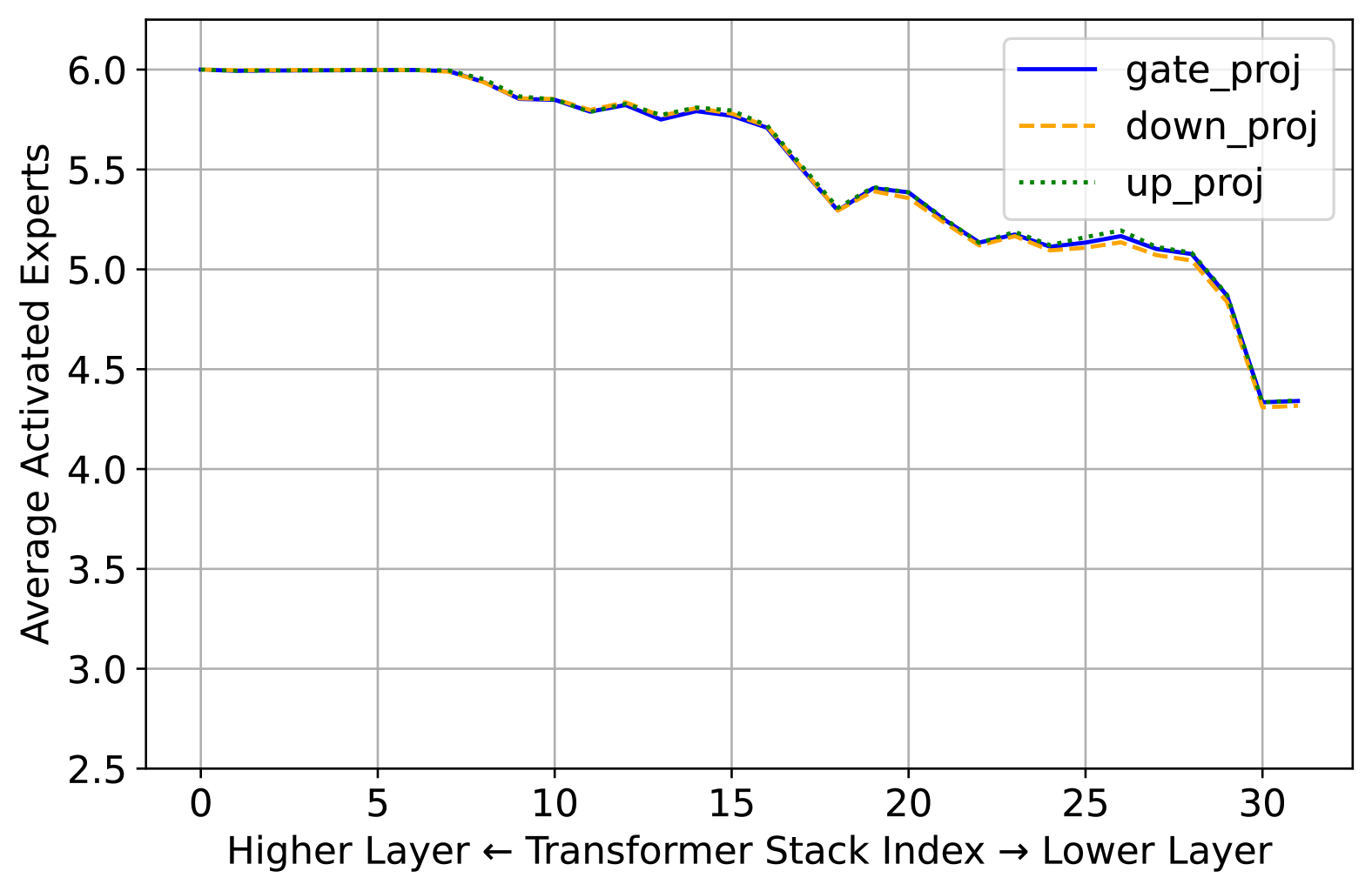
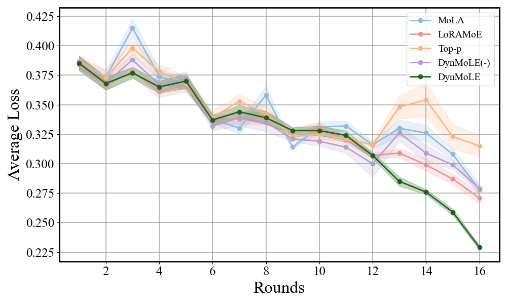
We evaluated the flexibility of \model and the Top-p method on the ARC-c dataset (as shown in Figure 6). Similar to Top-p, \model demonstrates comparable performance across the three projections. However, \model activates the appropriate number of experts earlier and more comprehensively in response to router uncertainty.
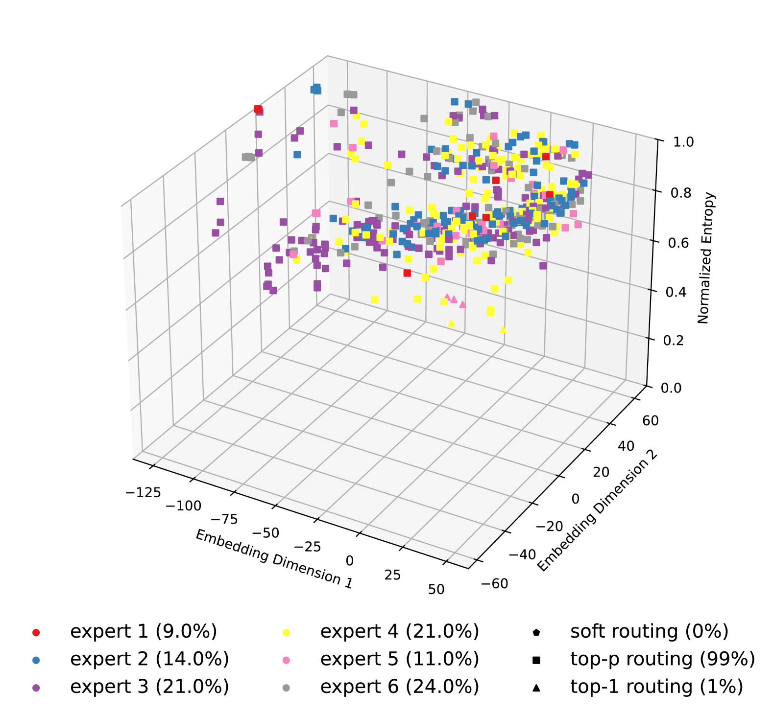
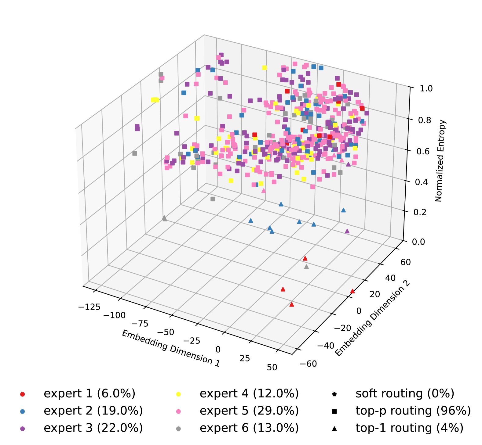
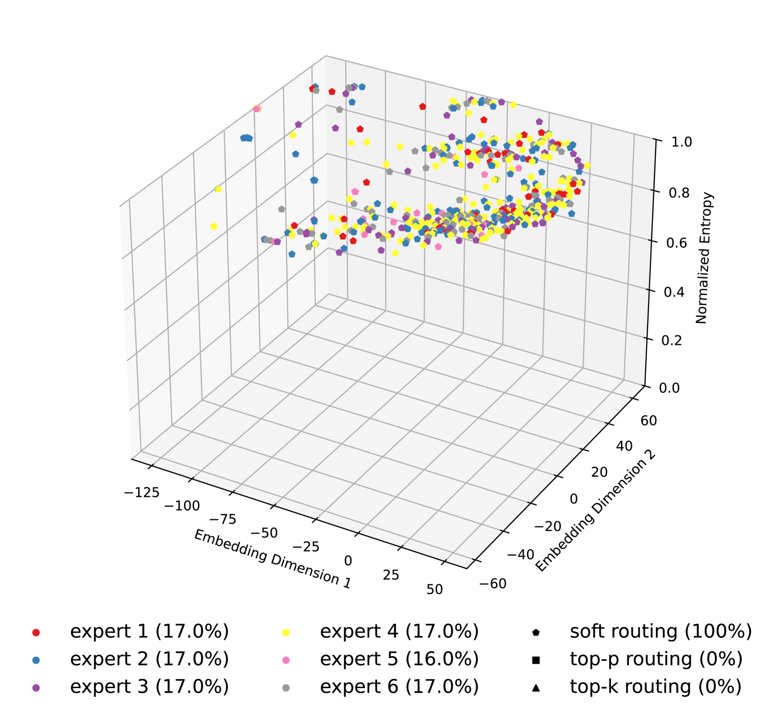
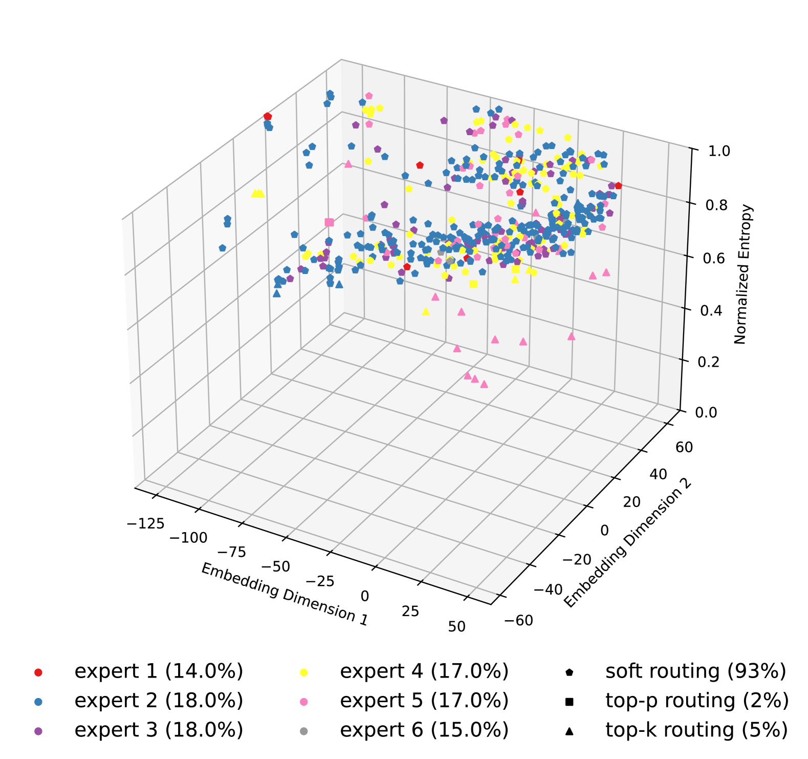
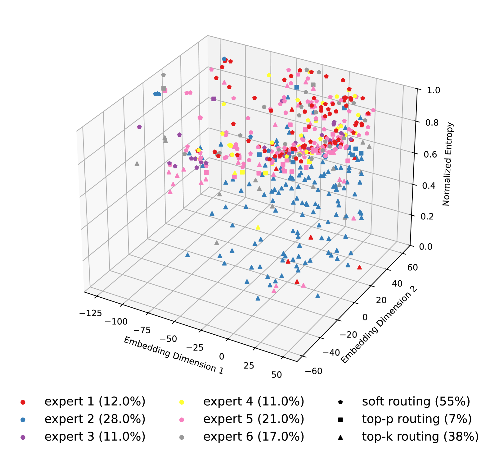
A.6 Word Embedding
As shown in Figure 7, we present a visualization comparing token allocation between the Top-P routing strategy (Huang et al., 2024) and our proposed \model approach. We embedded 2D visualized word tokens from 10 randomly selected sentences, coloring them based on their most confidently routed expert index from the 1st, 16th, and 32nd Transformer layers, and projected them into 3D space using their normalized entropy. The percentage distribution of routing strategies is shown for each method. Compared to Top-P, \model more efficiently routes tokens with similar entropy to similar experts, resulting in significantly lower average entropy and a more balanced load across experts, as reflected in the more even distribution across layers.