Data Sourcing Random Access using
Semantic Queries for Massive IoT Scenarios

Abstract

Efficiently retrieving relevant data from massive Internet of Things (IoT) networks is essential for downstream tasks such as machine learning. This paper addresses this challenge by proposing a novel data sourcing protocol that combines semantic queries and random access. The key idea is that the destination node broadcasts a semantic query describing the desired information, and the sensors that have data matching the query then respond by transmitting their observations over a shared random access channel, for example to perform joint inference at the destination. However, this approach introduces a tradeoff between maximizing the retrieval of relevant data and minimizing data loss due to collisions on the shared channel. We analyze this tradeoff under a tractable Gaussian mixture model and optimize the semantic matching threshold to maximize the number of relevant retrieved observations. The protocol and the analysis are then extended to handle a more realistic neural network-based model for complex sensing. Under both models, experimental results in classification scenarios demonstrate that the proposed protocol is superior to traditional random access, and achieves a near-optimal balance between inference accuracy and the probability of missed detection, highlighting its effectiveness for semantic query-based data sourcing in massive IoT networks.

I Introduction

Wireless Internet of Things (IoT) devices are becoming increasingly advanced and equipped with a multitude of sensors, allowing them to monitor complex signals, such as images, video, and audio/speech [2]. Enhanced by advanced processing in the cloud or on an edge server, usually relying on machine learning (ML) and artificial intelligence (AI), IoT devices can be used for a wide range of applications, such as autonomous control, surveillance, detection of accidents, fault detection in critical infrastructure (e.g., smart grids and water networks), and many others [3, 4]. However, collecting the massive, continuous stream of data produced by the sensors over a capacity-constrained wireless channel while considering the strict power constraints of the IoT devices poses a significant challenge. This task is further complicated by the fact that the data collected by individual sensors may not always be relevant for applications at the destination node [5, 6]. For instance, a wildlife monitoring application may only be interested in tracking a particular animal at a given time. Similarly, data relevant for an industrial monitoring application may depend on data observed by other sensors. For instance, a sudden temperature spike in a machine component might only be relevant if accompanied by abnormal vibration readings from other sensors.

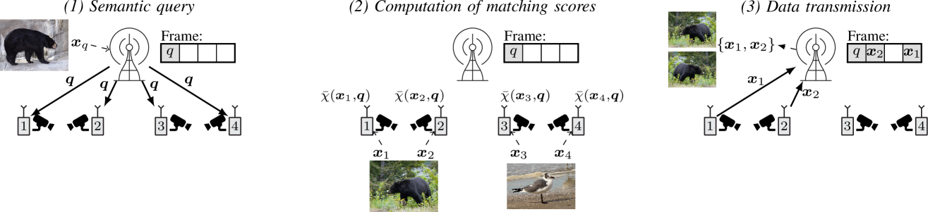
Figure 1: The proposed protocol for data sourcing random access. (1) The edge server broadcasts a semantic query, $\bm{q}$, in the first frame slot based on the query example $\bm{x}_{q}$; (2) Each device computes a matching score $\bar{\chi}(\bm{x}_{m},\bm{q})$ characterizing how well its observation $\bm{x}_{m}$ matches the query; (3) The devices whose matching score exceeds a threshold transmit their observations in the remaining slots using a random access protocol, and the edge server executes an application, such as inference, based on the received observations.

Conventional IoT protocols rely on device-initiated push communication, such as periodic reporting through random access, and are often agnostic to data relevance and significance, which can lead to inefficient use of resources [7]. Furthermore, even if the devices implement more intelligent transmission policies that depend on their data content, the devices have limited information about the global state of the network and the significance of the data within the context of the application, preventing them from making optimal transmission decisions. Alternatively, communication can be pull-based, where the destination node actively requests data from specific devices based on what is needed by the application. The simplest form of pull-based communication is scheduling, where individual devices are granted dedicated, contention-free resources to transmit their observations. However, with generic pull-based communication, the destination and scheduler are unaware of the actual data available at the devices, creating the risk of requesting data that ultimately turns out to be irrelevant.

To minimize irrelevant transmissions, this paper considers query-driven communication, which is a specific instance of pull-based communication. Rather than scheduling individual devices, the destination node transmits a query that specifies which kind of information the application seeks to obtain. This brings the advantage of collecting only relevant data, and is an attractive scheme when only a small fraction of the sensors produce relevant data, and when the sensors with relevant data are hard to predict. Since the devices with relevant information form a random subset, the query in the downlink is followed by random access transmission of the sensing data. This introduces the challenge of balancing the probability of missed detection (MD) and false alarm (FA) while minimizing the risk of data loss caused by random access collisions. In this paper, we analyze this tradeoff and optimize the protocol parameters to maximize the performance.

As an illustration, consider an IoT network of cameras deployed for wildlife monitoring. To track, for instance, a reported wild bear, a conventional push-based communication where cameras transmit images periodically, or, e.g., when there is movement, suffers from low capture probability and potential staleness of information. Conversely, in a query-driven, pull-based approach, the edge server first broadcasts a “bear” query to the devices, e.g., generated using a “query-by-example” approach [8] as illustrated Fig. 1. The cameras then transmit only upon observing an image whose matching score to the received query is sufficiently high, resulting in higher efficiency and timeliness. The end objective could, for instance, be to track the location of the bear, or to identify or classify the specific bear. We will consider both cases in this paper.

Previous works have explored various ways to incorporate data relevance in transmission policies. Recently, metrics like age of information (AoI) and its variants [9, 10, 11, 12] have been used in both push and pull communication to ensure relevance of the collected data by taking into account its timeliness at the destination node. However, timeliness may not be sufficient to quantify data relevance for all types of applications, such as the ones mentioned above. Furthermore, these works often rely on simple data models at the devices, or require detailed, continuously updated state information at the destination, which is challenging in practice, especially when communication is infrequent. Another recent direction is semantic and goal-oriented communication [5, 6, 13], which aims to optimize data transmission by considering the meaning and purpose of the communicated information at the destination. Semantic and goal-oriented communication has previously been applied to filter streaming IoT sensing data, where individual devices assess the semantic importance of their data [14]. As mentioned earlier, this approach is constrained by the lack of information available at the devices.

The concept of query-driven communication has been considered in, e.g., in-network query processing, where logical queries are used to filter data [15, 16]. Other examples include the use of content-based wake-up radios to collect the top-$k$ values in a sensor network [17]. Related to semantic filtering, [18] proposes to occasionally transmit ML models to the devices to enable them to locally assess the relevance of their observations. This approach can be seen as a special case of our work, in which the ML models serve as (large) queries. Closest to our work is the concept of semantic data sourcing, which was introduced in [19] and further analyzed in [20]. As in this paper, the concept in [19, 20] relies on a semantic query that summarizes the desired information and enables each device to decide the relevance of its data. Based on the query and their current sensing data, each device computes a matching score, which is sent back to the edge server. The edge server then schedules a subset of the devices to transmit their full observations. By leveraging ML to construct the query, the authors demonstrate how semantic data sourcing can reduce the communication efficiency of numerous edge-AI use cases.

The main limitation of the protocol in [19, 20] is the need to collect matching scores from all devices, which is costly when the number of devices is large. This paper addresses this limitation by proposing a joint data sourcing and random access protocol where devices with a matching score exceeding a predefined threshold directly transmit their observations over a shared random access channel using general irregular repetition slotted ALOHA (IRSA) [21] (see Fig. 1). IRSA represents a modern massive random access scheme and generalizes conventional slotted ALOHA, which is widely used in commercially available IoT protocols [22]. Following random access, the edge server can then process the received observations for tasks, such as machine learning inference as in [19, 20]. While our primary objective is joint classification (e.g., a multi-view inference scenario [23]), we will also characterize more general retrieval quantities such as the probability of MD and FA.

Our main contributions and findings can be summarized as follows: (i) We propose the concept of data sourcing random access using semantic queries, which integrates pull-based semantic data sourcing with contention-based IRSA random access in the uplink. (ii) We characterize the fundamental tradeoffs between the observation discrimination gain, query dimensionality, MD and FA by analyzing the problem under a tractable Gaussian mixture model (GMM) for sensing. (iii) We propose an efficient method to optimize the matching score threshold to minimize the probability of missed detection. The numerical results show that the proposed method provides near-optimal threshold selection across several tasks. (iv) We present experiments that show that the insights obtained using the GMM are, generally, consistent with results observed from a more realistic convolutional neural network (CNN)-based model applied to visual sensing data.

The remainder of the paper is organized as follows. Section II presents the general setup and the system model. We analyze the system under GMM sensing in Section III, and optimize the matching score in Section IV. In Section V, we extend the framework to a more realistic ML-based sensing scenario, in which sensors observe images and the edge server aims to perform image classification. Section VI presents numerical results, and the paper is concluded in Section VII.

Notation: Vectors are represented as column vectors and written in lowercase boldface (e.g., $\bm{x}$), while matrices are written in uppercase boldface (e.g., $\mathbf{X}$). $\Gamma(\cdot)$, $\Gamma(\cdot,\cdot)$, and $Q_{M}(\alpha,\beta)$ denote the gamma function, the upper incomplete gamma function, and the generalized Marcum Q-function of order $M$, respectively. The multivariate Gaussian probability density function (PDF) with mean $\bm{\mu}$ and covariance matrix $\bm{\Sigma}$ evaluated at $\bm{x}$ is written $\mathcal{N}(\bm{x}|\bm{\mu},\bm{\Sigma})$. $\mathbbm{1}[\cdot]$ is the indicator function, evaluating to $1$ for a true argument and $0$ otherwise.

II System Model

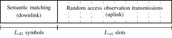
Figure 2: The considered frame structure containing semantic matching followed by random access observation transmission.

We consider a scenario with $M$ IoT sensor devices connected through a wireless link to an edge server. Time is divided into independent recurring frames, each comprising a semantic matching phase and a random access phase, as depicted in Fig. 2. In the semantic matching phase, the edge server broadcasts a semantic query based on a given query example [8], with the aim of allowing each of the IoT devices to determine whether its current sensing data are relevant for the server. The devices that conclude from the semantic matching that their sensing data are relevant transmit them over a random access channel to the edge server. While our protocol can be applied to many applications, we assume that the overall goal is to retrieve and then perform joint classification of the sensor observations that are relevant, according to a certain criterion, to the query example. We present the sensing, inference, and communication models, as well as the considered performance metrics in the sequel.

II-A Sensing and Inference Model

We assume that the query example at the edge server represents an unobservable query class $z_{q}\in\mathcal{Z}=\{1,2,\ldots,|\mathcal{Z}|\}$ drawn uniformly at random from the set of classes $\mathcal{Z}$. Since $\mathcal{Z}$ can be very large in practice, we assume that it is known only to the edge server and not to the IoT devices. Based on the query example, the edge server extracts a query feature vector $\bm{x}_{q}\in\mathbb{R}^{d}$, e.g., using a neural network, which it uses to construct the semantic query (elaborated later). Similarly, each IoT device, indexed by $m=1,2,\ldots,M$, produces a feature vector $\bm{x}_{m}\in\mathbb{R}^{d}$ representing its sensed data of some unobservable class $z_{m}\in\mathcal{Z}$. We assume that each of the $M$ devices produces a feature vector of the query class $z_{q}$ with probability $p_{\mathrm{pos}}$, or otherwise produces a feature vector of a different class drawn uniformly from the set of remaining classes $\mathcal{Z}\setminus z_{q}$. Letting $\mathsf{Z}=(z_{q},z_{1},\ldots,z_{M})$ be the the query class and the device classes, the joint class distribution can be written

$$p(\mathsf{Z})=\frac{1}{|\mathcal{Z}|}\prod_{m=1}^{M}\left(p_{\mathrm{pos}}\right)^{\mathbbm{1}[z_{m}=z_{q}]}\left(\frac{1-p_{\mathrm{pos}}}{|\mathcal{Z}|-1}\right)^{\mathbbm{1}[z_{m}\neq z_{q}]}.$$

We denote the indices of the devices that observe class $z\in\mathcal{Z}$ by $\mathcal{M}_{z}$. To capture correlation between sensors observing the same class (e.g., as in multi-view sensing [23]), we assume that the feature vectors $\mathsf{X}=(\bm{x}_{q},\bm{x}_{1},\ldots,\bm{x}_{M})$ are drawn from the joint distribution

$$p(\mathsf{X}|\mathsf{Z})=p(\bm{x}_{q}|z_{q})\prod_{z=1}^{|\mathcal{Z}|}\int_{\kappa_{z}}\prod_{i\in\mathcal{M}_{z}}p(\bm{x}_{i}|\kappa_{z})p(\kappa_{z}|z)\,\mathrm{d}\kappa_{z},$$ (1)

where $\kappa_{z}$ is a latent variable characterizing the correlation among the sensors observing class $z$.

After semantic matching and transmission, we assume that the edge server computes a fused feature vector from the received feature vectors, as

$$\bar{\bm{x}}=\frac{\sum_{m\in\mathcal{M}_{\mathrm{rx}}}\chi(\bm{x}_{m},\bm{x}_{q})\bm{x}_{m}}{\sum_{m^{\prime}\in\mathcal{M}_{\mathrm{rx}}}\chi(\bm{x}_{m^{\prime}},\bm{x}_{q})},$$ (2)

where $\mathcal{M}_{\mathrm{rx}}$ is the set of devices from which it has received feature vectors and $\chi(\bm{x}_{m},\bm{x}_{q})\geq 0$ is the weight given to feature $\bm{x}_{m}$ given the query $\bm{x}_{q}$. The weight function $\chi(\bm{x}_{m},\bm{x}_{q})$ is assumed to represent the relevance of the observation given the query, and depends on the specific problem. This type of feature fusion resembles an attention mechanism, and has been used previously in the literature [24, 25, 26]. We consider two specific sensing models as described next.

II-A1 GMM for Linear Classification

To get insights into the problem, we primarily focus on an analytically tractable Gaussian sensing model, where all feature vectors are drawn independently from Gaussian distributions conditioned on the observed classes as

$$p\left(\mathsf{X}|\mathsf{Z}\right)=\prod_{\bm{x}_{i}\in\mathsf{X}}\mathcal{N}(\bm{x}_{i}|\bm{\mu}_{z_{i}},\bm{\Sigma}).$$

Note that the means (or class centroids) are determined by the class observed by each sensor, $z_{i}$, while the covariance matrix $\bm{\Sigma}\in\mathbb{R}^{d\times d}$ is assumed to be the same for all classes. We assume that $\bm{\Sigma}$ is diagonalized with diagonal entries $C_{1,1},C_{2,2},\ldots,C_{d,d}$ (e.g., obtained using singular value decomposition). Note that the marginal feature vector distribution follows a GMM with density

$$p\left(\bm{x}_{i}\right)=\frac{1}{|\mathcal{Z}|}\sum_{z=1}^{|\mathcal{Z}|}\mathcal{N}(\bm{x}_{i}|\bm{\mu}_{z},\bm{\Sigma}).$$ (3)

As relevancy metric, we consider the exponential squared Mahalanobis distance between a feature vector $\bm{x}_{m}$ and the query feature vector $\bm{x}_{q}$, defined as

$$\chi(\bm{x}_{m},\bm{x}_{q}) =e^{-\frac{1}{d}\xi_{\bm{\Sigma}}(\bm{x}_{m},\bm{x}_{q})},$$ (4)

where

$$\xi_{\bm{\Sigma}}(\bm{a},\bm{b}) =\left(\bm{a}-\bm{b}\right)^{T}\bm{\Sigma}^{-1}\left(\bm{a}-\bm{b}\right)$$

$$=\sum_{n=1}^{d}\frac{(\bm{a}[n]-\bm{b}[n])^{2}}{C_{n,n}}$$ (5)

is the squared Mahalanobis distance between $\bm{a}$ and $\bm{b}$ under covariance matrix $\bm{\Sigma}$. Note that the factor $(1/d)$ in the exponent of Eq. 4 normalizes the exponent by the variance of the Mahalanobis distance when $\bm{x}_{m}$ and $\bm{x}_{q}$ are drawn from the same class.

Complete maximum a posteriori classification of the fused feature vector is challenging because of the correlation introduced by the weight functions. Instead, we treat the fused feature vector $\bar{\bm{x}}$ as a weighted average of $|\mathcal{M}_{\mathrm{rx}}|$ feature vectors drawn from the same class under the assumption that the feature weights are independent of the feature vectors themselves. Under this assumption, the fused feature vector $\bar{\bm{x}}$ is drawn from a GMM equivalent to that in Eq. 3 with class means

$$\widehat{\bm{\mu}}_{z} =\frac{\sum_{m\in\mathcal{M}_{\mathrm{rx}}}\chi(\bm{x}_{m},\bm{x}_{q})\bm{\mu}_{z}}{\sum_{m^{\prime}\in\mathcal{M}_{\mathrm{rx}}}\chi(\bm{x}_{m^{\prime}},\bm{x}_{q})}=\bm{\mu}_{z},$$

and covariance

$$\widehat{\bm{\Sigma}} =\sum_{m\in\mathcal{M}_{\mathrm{rx}}}\left(\frac{\chi(\bm{x}_{m},\bm{x}_{q})}{\sum_{m^{\prime}\in\mathcal{M}_{\mathrm{rx}}}\chi(\bm{x}_{m^{\prime}},\bm{x}_{q})}\right)^{2}\bm{\Sigma}$$

$$=\left(\frac{\sum_{m\in\mathcal{M}_{\mathrm{rx}}}\chi(\bm{x}_{m},\bm{x}_{q})^{2}}{\left(\sum_{m^{\prime}\in\mathcal{M}_{\mathrm{rx}}}\chi(\bm{x}_{m^{\prime}},\bm{x}_{q})\right)^{2}}\right)\bm{\Sigma}.$$

Note that this choice of model ensures that the variance of the individual feature entries decreases as the number of observations increases. The a posteriori distribution is then

$$p_{\mathrm{pred}}(z|\bar{\bm{x}}) =\frac{\mathcal{N}(\bar{\bm{x}}|\bm{\mu}_{z},\widehat{\bm{\Sigma}})}{\sum_{z^{\prime}=1}^{|\mathcal{Z}|}\mathcal{N}(\bar{\bm{x}}|\bm{\mu}_{z^{\prime}},\widehat{\bm{\Sigma}})}=\frac{e^{-\frac{1}{2}\xi_{\widehat{\bm{\Sigma}}}(\bar{\bm{x}},\bm{\mu}_{z})}}{\sum_{z^{\prime}=1}^{|\mathcal{Z}|}e^{-\frac{1}{2}\xi_{\widehat{\bm{\Sigma}}}(\bar{\bm{x}},\bm{\mu}_{z^{\prime}})}},$$

from which the maximum a posteriori class estimate can be obtained as

$$\hat{z}=\operatorname*{arg\,max}_{z\in\mathcal{Z}}p_{\mathrm{pred}}(z|\bar{\bm{x}}).$$

II-A2 General Model for CNN Classification

For a more realistic but analytically intractable evaluation, we also consider a general CNN sensing model for nonlinear classification. Here, each feature vector $\bm{x}_{i}\in\mathsf{X}$ (including the query feature vector) is extracted from an input image $\tilde{x}_{i}$ using an encoder CNN as $\bm{x}_{i}=f_{\mathrm{enc}}(\tilde{x}_{i})$. We will assume that all sensors observing a given class observe different views of the same object, e.g., from various angles or under different light conditions. More formally, we will assume that the input images $\tilde{\mathsf{X}}=(\tilde{x}_{q},\tilde{x}_{1},\ldots,\tilde{x}_{M})$ are drawn from the distribution

$$p(\tilde{\mathsf{X}}|\mathsf{Z})=p(\tilde{x}_{q}|z_{q})\prod_{z=1}^{|\mathcal{Z}|}\int_{\kappa_{z}}\prod_{i\in\mathcal{M}_{z}}p(\tilde{x}_{i}|\kappa_{z})p(\kappa_{z}|z)\,\mathrm{d}\kappa_{z}.$$ (6)

Under this assumption, the set of feature vectors $\mathsf{X}=(f_{\mathrm{enc}}(\tilde{x}_{q}),f_{\mathrm{enc}}(\tilde{x}_{1}),\ldots,f_{\mathrm{enc}}(\tilde{x}_{M}))$ extracted from images $\tilde{\mathsf{X}}$ follows a distribution of the form in Eq. 1.

For classification, the edge server employs a neural network that is composed of feature fusion followed by a classifier. The feature fusion learns the relevancy metric $\chi(\bm{x}_{m},\bm{x}_{q})$ and computes a fused feature vector $\bar{\bm{x}}$ as in Eq. 2. The fused feature vector $\bar{\bm{x}}$ is passed to a neural network classifier $f_{\mathrm{ser}}(\cdot)$, which outputs a $|\mathcal{Z}|$-dimensional vector through a softmax activation function, so that which each entry approximates $p_{\mathrm{pred}}(z|\bar{\bm{x}})$. The class estimate $\hat{z}$ is then obtained as

$$\hat{z}=\operatorname*{arg\,max}_{z\in\mathcal{Z}}\left[f_{\mathrm{ser}}(\bar{\bm{x}})\right]_{z},$$ (7)

where $\left[f_{\mathrm{ser}}(\bar{\bm{x}})\right]_{z}$ denotes the $z$-th entry of the vector $f_{\mathrm{ser}}(\bar{\bm{x}})$.

II-B Communication Model

II-B1 Semantic Matching (Downlink)

In the semantic matching phase, the edge server constructs an $l$-dimensional semantic query vector $\bm{q}\in\mathbb{R}^{l}$ from its query feature vector $\bm{x}_{q}$. We assume that the dimension of the query vector is less than that of the query feature vector, i.e., $l\leq d$. The query vector is transmitted to all devices with the purpose of allowing each device to compute a matching score $\bar{\chi}(\bm{x}_{m},\bm{q})\geq 0$ that approximates the relevancy of its sensed feature vector given the query feature vector, i.e.,

$$\bar{\chi}(\bm{x}_{m},\bm{q})\approx\chi(\bm{x}_{m},\bm{x}_{q}).$$

We assume that each entry of the query vector is quantized to sufficient number of bits, $\bar{Q}$, such that the quantization noise is negligible. The resulting $l\bar{Q}$ bits are transmitted using $L_{\mathrm{dl}}$ (complex) symbols, resulting in a transmission rate of $R_{\mathrm{dl}}=l\bar{Q}/L_{\mathrm{dl}}$ bits/symbol. We assume independent Rayleigh block-fading channels to each device, and for simplicity, we will assume that all devices have the same average signal-to-noise ratio (SNR) $\gamma$. The query transmission error probabilities experienced by the devices are then independent and given by the outage probability

$$p_{\mathrm{err}}^{\mathrm{dl}}=1-\exp\left(\frac{-\left(2^{R_{\mathrm{dl}}}-1\right)}{\gamma}\right).$$

The devices that successfully receive the query will perform threshold-based semantic matching, i.e., they will assume that their observation matches the query whenever $\bar{\chi}(\bm{x}_{m},\bm{q})\geq\tau$ for some predefined threshold $\tau\geq 0$. We assume that devices that experience outage refrain from transmitting in the uplink.

II-B2 Random Access Observation Transmission (Uplink)

The devices with matching observations transmit their observations to the server over a shared IRSA random access channel comprising $L_{\mathrm{ul}}$ transmission slots. In IRSA, each of the transmitting devices transmits a random number $L_{m}$ of identical packet replicas in slots selected uniformly at random without replacement among all $L_{\mathrm{ul}}$ slots. The number of replicas is drawn from the common degree distribution $\{\Lambda_{\ell}\}_{\ell=0}^{L_{\mathrm{ul}}}$, where $\Lambda_{\ell}=\Pr(L_{m}=\ell)$. Following the literature on IRSA (see, e.g., [21]), we will represent the degree distribution in compact polynomial form as $\Lambda(x)=\sum_{\ell=1}^{L_{\mathrm{ul}}}\Lambda_{\ell}x^{\ell}$. The degree distribution is assumed to be given.

At the end of the frame, the receiver decodes the packets iteratively using successive interference cancellation. Specifically, in each iteration, the receiver decodes packets in slots with only a single transmission, and then subtracts the remaining replicas of the decoded packets from their respective slots. This process is repeated until no slots with a single transmission remains, and any remaining transmissions are assumed to have failed. Note that $\Lambda(x)=x$ corresponds to conventional slotted ALOHA with a single replica. Averaging over the random replicas, the transmission failure probability is the same for all transmitting devices and denoted as $p_{\mathrm{err}}^{\mathrm{ul}}$.

II-C Performance Metrics

Our overall goal is to maximize the expected inference (or classification) accuracy defined as

Inference accuracy $$=\frac{1}{|\mathcal{Z}|}\sum_{z_{q}=1}^{|\mathcal{Z}|}\operatorname*{\mathbb{E}}\left[\Pr(\hat{h}=z_{q}|z_{q})\,\middle|\,z_{q}\right],$$ (8)

where the expectation is over the observed feature vectors and the uplink transmission.

In addition to inference accuracy, we are also interested in the overall retrieval performance, characterized by the probability of MD and FA. The probability of MD, $\varepsilon_{\mathrm{MD}}$, is defined as the probability that a device that observes the query class is not among the set of received observations, while the probability of FA, $\varepsilon_{\mathrm{FA}}$, is defined as the probability that a device that does not observe the query class is among the set of received observations. Formally,

$$\varepsilon_{\mathrm{MD}}\! =\!\frac{1}{|\mathcal{Z}|}\!\sum_{z_{q}=1}^{|\mathcal{Z}|}\operatorname*{\mathbb{E}}\!\left[\frac{1}{|\mathcal{M}_{z_{q}}|}\!\sum_{m_{i}\in\mathcal{M}_{z_{q}}}\!\Pr(m_{i}\!\notin\!\mathcal{M}_{\mathrm{rx}})\,\middle|\,z_{q}\right],$$ (9)

$$\varepsilon_{\mathrm{FA}}\! =\!\frac{1}{|\mathcal{Z}|}\!\sum_{z_{q}=1}^{|\mathcal{Z}|}\operatorname*{\mathbb{E}}\!\left[\frac{1}{|\mathcal{M}_{\mathrm{rx}}|}\!\sum_{m_{i}\in\mathcal{M}_{\mathrm{rx}}}\!\Pr(m_{i}\!\notin\!\mathcal{M}_{z_{q}})\,\middle|\,z_{q}\right],$$ (10)

where both expectations are the sets $\mathcal{M}_{z_{q}}$ and $\mathcal{M}_{\mathrm{rx}}$.

III Semantic Matching Design

In this section, we present and analyze the proposed semantic matching phase for the GMM in details. We first describe the proposed query and matching design, which relies on linear projections, and then consider the problem of selecting the projection matrix.

III-A Query and Matching Design

Recall that our aim is to construct a low-dimensional query vector $\bm{q}\in\mathbb{R}^{l}$ that allows devices to compute a matching score $\bar{\chi}(\bm{x}_{m},\bm{q})$ that approximates the relevancy score in Eq. 4. For analytical tractability, we will construct the query as a linear orthogonal projection of the query feature vector. First, the squared Mahalanobis distance in Eq. 5 can be equivalently written

$$\xi_{\bm{\Sigma}}(\bm{x}_{m},\bm{x}_{q})=\|\bm{\Sigma}^{-\frac{1}{2}}\bm{x}_{m}-\bm{\Sigma}^{-\frac{1}{2}}\bm{x}_{q}\|_{2}^{2}.$$

Let $\mathbf{P}_{l}\in\mathbb{R}^{l\times d}$ denote the matrix that defines the projection to the $l$-dimensional subspace satisfying $\mathbf{P}_{l}\mathbf{P}_{l}^{T}=\mathbf{I}_{l}$. We then approximate the squared Mahalanobis distance as

$$\xi_{\bm{\Sigma}}(\bm{x}_{m},\bm{x}_{q}) \approx(d/l)\|\mathbf{P}_{l}\bm{\Sigma}^{-\frac{1}{2}}\bm{x}_{m}-\mathbf{P}_{l}\bm{\Sigma}^{-\frac{1}{2}}\bm{x}_{q}\|_{2}^{2},$$ (11)

where $(\sqrt{d/l})$ is a normalization factor to compensate for the reduced dimensionality. Note that the approximation in Eq. 11 becomes an equality when $l=d$.

Under this approximation, we define the query vector $\bm{q}$ and a corresponding key vector $\bm{k}_{m}\in\mathbb{R}^{l}$ as

$$\bm{q} =(\sqrt{d/l})\mathbf{P}_{l}\bm{\Sigma}^{-\frac{1}{2}}\bm{x}_{q},$$ (12)

$$\bm{k}_{m} =(\sqrt{d/l})\mathbf{P}_{l}\bm{\Sigma}^{-\frac{1}{2}}\bm{x}_{m},\ m=1,\ldots,M.$$ (13)

Combining these definitions with Eqs. 4 and 11, we obtain the matching score as

$$\bar{\chi}(\bm{x}_{m},\bm{q})=e^{-\frac{1}{d}\|\bm{k}_{m}-\bm{q}\|_{2}^{2}},$$

where for simplicity we omit the dependency of $\bm{x}_{m}$ on $\bm{k}_{m}$. Note that $\bar{\chi}(\bm{x}_{m},\bm{q})$ is a monotonically decreasing function of the approximate squared Mahalanobis distance, and thus also of the approximated relevancy of the device feature vector.

The following lemma characterizes the resulting probabilities of MD and FA of semantic matching prior to the uplink phase, denoted as $\varepsilon_{\mathrm{MD},\mathrm{match}}(\tau)$ and $\varepsilon_{\mathrm{FA},\mathrm{match}}(\tau)$, respectively.

Lemma 1.

For fixed $p_{\mathrm{err}}^{\mathrm{dl}}$ and for any threshold $0<\tau\leq 1$, the probability of MD $\varepsilon_{\mathrm{MD},\mathrm{match}}(\tau)$ and FA $\varepsilon_{\mathrm{FA},\mathrm{match}}(\tau)$ in the semantic matching phase under the GMM are given as

$$\varepsilon_{\mathrm{MD},\mathrm{match}}(\tau) =1-(1-p_{\mathrm{err}}^{\mathrm{dl}})\left(1-\frac{\Gamma\left(l/2,\tilde{\tau}/4\right)}{\Gamma(l/2)}\right),$$ (14)

$$\varepsilon_{\mathrm{FA},\mathrm{match}}(\tau) =\left(1-p_{\mathrm{err}}^{\mathrm{dl}}\right)\bigg{[}1-\frac{2}{|\mathcal{Z}|(|\mathcal{Z}|-1)}$$

$$\quad\times\sum_{i=1}^{|\mathcal{Z}|}\sum_{j=i+1}^{|\mathcal{Z}|}Q_{\frac{l}{2}}\left(\sqrt{G_{i,j}(\mathbf{P}_{l})/2},\sqrt{\tilde{\tau}/2}\right)\bigg{]},$$ (15)

where $\tilde{\tau}=l\ln(1/\tau)$ and

$$G_{i,j}(\mathbf{P}_{l})=\left(\bm{\mu}_{i}-\bm{\mu}_{j}\right)^{T}\bm{\Sigma}^{-\frac{1}{2}}\mathbf{P}_{l}^{T}\mathbf{P}_{l}\bm{\Sigma}^{-\frac{1}{2}}\left(\bm{\mu}_{i}-\bm{\mu}_{j}\right).$$

Proof:

See Appendix A. ∎

The MD probability in Lemma 1 is a monotonically increasing function in $\tau$, while the FA is decreasing in $\tau$, revealing the tradeoff between MD and FA controlled by $\tau$. Furthermore, the FA probability is a monotonically increasing function of $G_{i,j}(\mathbf{P}_{l})$. This quantity is equivalent to the symmetric Kullback-Leibler (KL) divergence between the feature vector distributions of classes $i$ and $j$ in the reduced dimensionality space, and is often referred to as the discriminant gain since it represents the discernibility between the two classes [27]. Note that only the probability of FA depends on $\mathbf{P}_{l}$. Thus, for a fixed dimension $l$, the projection matrix $\mathbf{P}_{l}$ should be chosen to minimize the probability of FA, which we do next.

III-B Query Projection Optimization

In this section, we consider the problem of selecting the projection matrix $\mathbf{P}_{l}$ so as to minimize the probability of FA. However, direct optimization of $\varepsilon_{\mathrm{FA},\mathrm{match}}(\tau)$ is challenging because of the non-linearity introduced by $Q_{M}(\alpha,\beta)$, which has no closed form. Furthermore, because of this non-linearity, the matrix $\mathbf{P}_{l}$ that minimizes $\varepsilon_{\mathrm{FA},\mathrm{match}}(\tau)$ depends on the choice of the matching threshold $\tau$. This means that the optimal $\mathbf{P}_{l}$ needs to be computed and communicated to the devices (or stored) for each particular choice of $\tau$, which may not be desirable in practice. Instead, we propose the more pragmatic strategy to pick the $\mathbf{P}_{l}$ that maximizes the average discriminant gain $G_{i,j}(\mathbf{P}_{l})$ over all classes. This problem can be written:

$$\max_{\mathbf{P}_{l}\in\mathbb{R}^{l\times d}} \frac{2}{|\mathcal{Z}|(|\mathcal{Z}|-1)}\sum_{i=1}^{|\mathcal{Z}|}\sum_{j=i+1}^{|\mathcal{Z}|}G_{i,j}(\mathbf{P}_{l}),$$ (16)

s.t. $$\mathbf{P}_{l}\mathbf{P}_{l}^{T}=\mathbf{I}_{l}.$$

Since $\varepsilon_{\mathrm{FA},\mathrm{match}}(\tau)$ is monotonically decreasing in the pairwise discriminant gains as discussed above, it can be expected that the solution to Eq. 16 also performs well in terms of the FA probability across a wide range of thresholds $\tau$. Furthermore, the solution to Eq. 16 has a closed form, as stated in the following proposition.

Proposition 1.

Define $\mathbf{W}\in\mathbb{R}^{d\times d}$ as

$$\mathbf{W}=\sum_{i=1}^{|\mathcal{Z}|}\bm{\Sigma}^{-\frac{1}{2}}(\bm{\mu}_{i}-\bar{\bm{\mu}})(\bm{\mu}_{i}-\bar{\bm{\mu}})^{T}\bm{\Sigma}^{-\frac{1}{2}}$$

where $\bar{\bm{\mu}}=\frac{1}{|\mathcal{Z}|}\sum_{i=1}^{|\mathcal{Z}|}\bm{\mu}_{i}$, and let $\bm{v}_{1},\bm{v}_{2},\ldots,\bm{v}_{d}\in\mathbb{R}^{d}$ be the eigenvectors of $\mathbf{W}$ sorted in descending order by the magnitude of their corresponding eigenvalues. For any feature dimension $1\leq l\leq d$, the $\mathbf{P}_{l}$ that solves Eq. 16 is

$$\mathbf{P}_{l}=\begin{bmatrix}\bm{v}_{1}^{T}&\bm{v}_{2}^{T}&\cdots&\bm{v}_{l}^{T}\end{bmatrix}^{T}.$$

Proof:

See Appendix B. ∎

Proposition 1 is equivalent to applying Fisher’s linear discriminant analysis (LDA) [28], which finds the linear projection that maximizes the ratio between the between-class and the within-class variances. This is intuitive, since the motivation behind LDA and that of maximizing the discriminant gain are essentially the same, namely to be able to distinguish samples drawn from distinct classes.

IV Random Access Design

In this section, we extend the previous analysis to include the random access phase. This phase introduces a new aspect to the tradeoff between MD and FA. Specifically, while a low matching threshold $\tau$ increases the probability of retrieving the desired observations, it may lead to a large number of collisions in the random access phase caused by FA. On the other hand, a high matching threshold reduces the risk of FA, but increases the probability of MD. To balance this tradeoff, we aim to optimize the matching score threshold $\tau$ to maximize the end-to-end classification accuracy by taking into account both semantic matching and collisions in the random access phase.

Unfortunately, direct optimization of classification accuracy is challenging as it depends on the distribution of the weighted feature vector, which is hard to compute. Instead, we consider the MD probability as a proxy for classification accuracy, and seek to minimize the MD probability. This is in turn equivalent to maximizing the number of received true positive (TP) observations, denoted as $N_{\mathrm{TP}}=|\mathcal{M}_{z_{q}}\cap\mathcal{M}_{\mathrm{rx}}|$. Using this, the considered threshold selection problem can be stated:

$$\max_{\tau\in[0,1]} \operatorname*{\mathbb{E}}\left[N_{\mathrm{TP}}\,\middle|\,\tau\right],$$ (17)

where the expectation is over the feature vectors, the downlink query transmission, and the transmission of the matching observations over the random access channel in the uplink.

Computing the objective function in Eq. 17 is still intractable because of correlation among the matching observations caused by the common query feature vector. Therefore, we will seek an approximate solution by assuming that the devices observe independent query feature vectors drawn from the query class. In this case, the probability of a true positive transmission is the probability that a device observes the query class and its relevancy score is greater than $\tau$, which can be expressed using the result in Lemma 1 as

$$p_{\mathrm{TP,tx}}(\tau)=p_{\mathrm{pos}}\left(1-\varepsilon_{\mathrm{MD},\mathrm{match}}(\tau)\right).$$

Similarly, the probability of a FA transmission can be written

$$p_{\mathrm{FA,tx}}(\tau)=(1-p_{\mathrm{pos}})\varepsilon_{\mathrm{FA},\mathrm{match}}(\tau).$$

Under the assumption of independent queries introduced above, the total number of transmissions in the random access phase follows a binomial distribution with $M$ trials and success probability $p_{\mathrm{TP,tx}}(\tau)+p_{\mathrm{FA,tx}}(\tau)$. For large $M$, which is the regime of interest, this number can be accurately approximated as a Poisson distribution with rate $\bar{\lambda}(\tau)=M(p_{\mathrm{TP,tx}}(\tau)+p_{\mathrm{FA,tx}}(\tau))$. Furthermore, under this assumption we may write the number of TP transmissions and the number of FA transmissions as independent Poisson distributed random variables with rates

$$\bar{\lambda}_{\mathrm{TP}}(\tau) =Mp_{\mathrm{TP,tx}}(\tau),$$ (18)

$$\bar{\lambda}_{\mathrm{FA}}(\tau) =Mp_{\mathrm{FA,tx}}(\tau),$$ (19)

respectively, such that $\bar{\lambda}(\tau)=\bar{\lambda}_{\mathrm{TP}}(\tau)+\bar{\lambda}_{\mathrm{FA}}(\tau)$.

In the following, we first present the analysis of conventional slotted ALOHA (i.e., $\Lambda(x)=x$), for which a simple approximate solution can be obtained. We will then generalize the result to the case of IRSA, which requires more involved approximations.

IV-A Conventional Slotted ALOHA

In conventional slotted ALOHA, transmission errors occur if another device transmits in the same slot. For Poisson arrivals and $L_{\mathrm{ul}}$ slots, this happens with probability

$$p_{\mathrm{err}}^{\mathrm{ul}}(\tau)=1-e^{-\bar{\lambda}(\tau)/L_{\mathrm{ul}}}.$$ (20)

The number of received true positive observations can then be approximated as

$$\operatorname*{\mathbb{E}}\left[N_{\mathrm{TP}}\,\middle|\,\tau\right]\approx\bar{\lambda}_{\mathrm{TP}}(\tau)\left(1-p_{\mathrm{err}}^{\mathrm{ul}}(\tau)\right),$$ (21)

where the approximation comes from the assumption that devices receive independent queries and from the Poisson approximation. The optimal $\tau$ that maximizes the right-hand side of Eq. 21 is presented in the following proposition.

Proposition 2.

For $l\geq 1$ and $L_{\mathrm{ul}}>0$, there exists a unique threshold $0<\tau\leq 1$ that maximizes the expected number of received true positive observations under the simplifying assumptions defined above. Furthermore, defining $\tilde{\tau}=l\ln(1/\tau)$, the optimal $\tau$ is the solution to

$$L_{\mathrm{ul}}-M(1-p_{\mathrm{err}}^{\mathrm{dl}})\gamma\left(\frac{l}{2},\frac{\tilde{\tau}}{4}\right)\\ \times\left(p_{\mathrm{pos}}+\frac{(1-p_{\mathrm{pos}})2^{l-1}\Gamma(l/2)}{|\mathcal{Z}|(|\mathcal{Z}|-1)}\phi\left(\tilde{\tau}\right)\right)=0,$$ (22)

where

$$\phi\left(\tilde{\tau}\right)=\tilde{\tau}^{1/2-l/4}\sum_{i=1}^{|\mathcal{Z}|}\sum_{j=i+1}^{|\mathcal{Z}|}\bigg{[}\frac{e^{-\frac{1}{4}G_{i,j}(\mathbf{P}_{l})}}{G_{i,j}(\mathbf{P}_{l})^{l/4-1/2}}\\ \times I_{l/2-1}\left(\frac{1}{2}\sqrt{G_{i,j}(\mathbf{P}_{l})\tilde{\tau}}\right)\bigg{]},$$

and $\gamma(s,x)$ and $I_{n}(x)$ are the lower incomplete gamma function and the modified Bessel function of the first kind, respectively.

Proof:

See Appendix C. ∎

The left-hand side of Eq. 22 is an increasing function of $\tau$, and thus the optimal $\tau$ can be solved efficiently using standard root-finding algorithms, such as bisection search. Once the optimal $\tau$ has been obtained, the probability of MD and FA as defined in Eqs. 9 and 10 can be approximated by combining the results in Lemma 1 with Eq. 20:

$$\varepsilon_{\mathrm{MD}} \approx\varepsilon_{\mathrm{MD},\mathrm{match}}(\tau)+p_{\mathrm{err}}^{\mathrm{ul}}(\tau)\left(1-\varepsilon_{\mathrm{MD},\mathrm{match}}(\tau)\right),$$ (23)

$$\varepsilon_{\mathrm{FA}} \approx\left(1-p_{\mathrm{err}}^{\mathrm{ul}}(\tau)\right)\varepsilon_{\mathrm{FA},\mathrm{match}}(\tau).$$ (24)

IV-B Irregular Repetition Slotted ALOHA

While the performance of conventional ALOHA is severely limited by collisions, IRSA can support a much larger number of devices with the same number of slots by allowing multiple repetitions and successive interference cancellation [21]. However, the analysis of IRSA is more involved, and the error probability cannot be expressed in closed-form. Instead, we will resort to approximations proposed in [29, 30], which have been applied with success to a wide range of scenarios, e.g., [22, 31]. These approximations rely on the fact that the error probability exhibits an error-floor regime for small frame loads (defined as $\bar{\lambda}(\tau)/L_{\mathrm{ul}}$), and a waterfall regime for large frame loads, which can be approximated separately. As in [22], we will approximate the total error probability as the sum of the approximations in the two regimes, i.e.,

$$p_{\mathrm{err}}^{\mathrm{ul}}(\tau)\approx p_{\mathrm{err},\mathrm{ef}}^{\mathrm{ul}}(\tau)+p_{\mathrm{err},\mathrm{wf}}^{\mathrm{ul}}(\tau),$$ (25)

where $p_{\mathrm{err},\mathrm{ef}}^{\mathrm{ul}}(\tau)$ and $p_{\mathrm{err},\mathrm{wf}}^{\mathrm{ul}}(\tau)$ are approximations of the error probability in the error-floor and in the waterfall regions, respectively. The waterfall approximation is [30]

$$p_{\mathrm{err},\mathrm{wf}}^{\mathrm{ul}}(\tau)=\alpha_{1}Q\left(\frac{\sqrt{L_{\mathrm{ul}}}\left(\alpha_{2}-\alpha_{3}L_{\mathrm{ul}}^{-2/3}-\bar{\lambda}(\tau)/L_{\mathrm{ul}}\right)}{\sqrt{\alpha_{0}^{2}+\bar{\lambda}(\tau)/L_{\mathrm{ul}}}}\right),$$

where $\alpha_{0},\alpha_{1},\alpha_{2},\alpha_{3}\in\mathbb{R}$ are constants that depend on the specific degree distribution $\Lambda(x)$ and obtained through numerical analysis of the decoding process. The error probability in the error-floor regime is approximated as [29]

$$p_{\mathrm{err},\mathrm{ef}}^{\mathrm{ul}}(\tau)$$

$$\!=\!\sum_{s=1}^{A}\phi(s,\tau)\bm{\nu}[s]\bm{\beta}_{0}[s]\binom{L_{\mathrm{ul}}}{\bm{\beta}_{1}[s]}\!\prod_{\ell=1}^{L_{\mathrm{ul}}}\frac{\Lambda_{\ell}^{\bm{\nu}_{\ell}[s]}}{\bm{\nu}_{\ell}[s]!}\binom{L_{\mathrm{ul}}}{\ell}^{-\bm{\nu}_{\ell}[s]},$$ (26)

where

$$\phi(s,\tau)=\sum_{k=0}^{\bm{\nu}[s]-1}(-1)^{\bm{\nu}[s]-1+k}\bar{\lambda}(\tau)^{k}\frac{(\bm{\nu}[s]-1)!}{k!}.$$

The constants $A\in\mathbb{Z}$, $\bm{\nu}_{\ell}\in\mathbb{R}^{|\mathcal{A}|},\ell=1,2,\ldots,L_{\mathrm{ul}}$, as well as $\bm{\beta}_{0},\bm{\beta}_{1}\in\mathbb{R}^{|\mathcal{A}|}$ depend on the specific degree distribution, and $\bm{\nu}=\sum_{\ell=1}^{L_{\mathrm{ul}}}\bm{\nu}_{\ell}$. For instance, for $\Lambda(x)=x^{3}$ Eq. 26 simplifies to

$$p_{\mathrm{err},\mathrm{ef}}^{\mathrm{ul}}(\tau)=\sum_{s=1}^{2}\frac{\phi(s,\tau)\bm{\nu}[s]\bm{\beta}_{0}[s]}{\bm{\nu}[s]!}\binom{L_{\mathrm{ul}}}{\bm{\beta}_{1}[s]}\binom{L_{\mathrm{ul}}}{3}^{-\bm{\nu}[s]},$$

and the parameters are given as $\alpha_{0}=0.497867$, $\alpha_{1}=0.784399$, $\alpha_{2}=0.818469$, $\alpha_{3}=0.964528$, $A=2$, $\bm{\nu}=(2,3)$, $\bm{\beta}_{0}=(1,24)$, $\bm{\beta}_{1}=(3,4)$ [22]. The resulting approximation is compared to simulations for $L_{\mathrm{ul}}\in\{25,50,100\}$ in Fig. 3 under the assumption of Poisson arrivals, showing that the approximation closely captures the trend of the error probability.

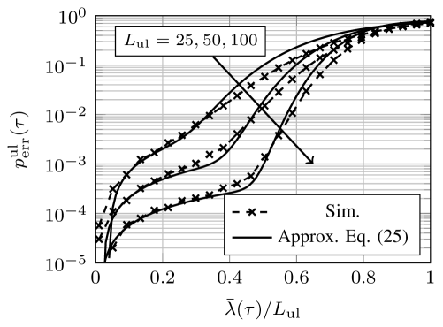
Figure 3: Comparison between simulated error probability and approximation (25) for $\Lambda(x)=x^{3}$ under Poisson arrivals.

We can now approximate the expected number of received true positive observations by using Eq. 25 in Eq. 21. The resulting approximation is accurate in the interval $\bar{\lambda}(\tau)\in[0,L_{\mathrm{ul}}]$. For $\bar{\lambda}(\tau)>L_{\mathrm{ul}}$, the error probability is close to $1$, and thus $\operatorname*{\mathbb{E}}\left[N_{\mathrm{TP}}\,\middle|\,\tau\right]$ is approximately zero. The threshold optimization problem can then be written

$$\max_{\tau\in[0,1]} \bar{\lambda}_{\mathrm{TP}}(\tau)\left(1-p_{\mathrm{err}}^{\mathrm{ul}}(\tau)\right)$$ (27)

s.t. $$\bar{\lambda}(\tau)<L_{\mathrm{ul}}.$$

Solving Eq. 27 analytically is hard because of the complexity of the approximation of $p_{\mathrm{err}}^{\mathrm{ul}}(\tau)$, and we resort to numerical optimization. To this end, we note that since $\bar{\lambda}(\tau)$ is monotonically decreasing in $\tau$, the constraint can be equivalently written as $\tau_{\mathrm{lb}}\leq\tau\leq 1$, where $\tau_{\mathrm{lb}}=\inf_{\tau\in[0,1]}\{\tau|\bar{\lambda}(\tau)\leq L_{\mathrm{ul}}\}$. Once $\tau_{\mathrm{lb}}$ has been determined, we maximize the objective function over $\tau\in[\tau_{\mathrm{lb}},1]$. However, since the objective function in Eq. 27 is not guaranteed to be convex, the optimization is sensitive to the initialization point. We address this issue by performing the optimization procedure multiple times with initial values of $\tau$ that are spaced at regular intervals over its domain, and then pick the best result across all initializations. While this generally does not guarantee to provide the globally optimal solution, experimental results suggest that the global optimum is always found even with only 10 initial values.

As for conventional ALOHA, the resulting MD and FA probabilities can be approximated using Eqs. 23 and 24 with the approximation in Eq. 25.

V CNN-Based Semantic Data Sourcing

The previous sections studied the semantic query and matching problem under the GMM. In this section, we demonstrate how the idea can be applied to the more realistic and general CNN-based sensing model. As in the GMM case, we propose to solve the matching problem by comparing the query broadcasted by the edge server to a local key constructed by each sensor. However, instead of designing the query and keys by hand for a specific relevancy function, we compute them using CNNs that we train to facilitate the end objective of maximizing the inference accuracy defined in Eq. 8. Note that the relevancy function is implicitly learned as part of the training. In the following, we first outline the query and key construction, and then explain how to optimize the matching score threshold.

V-A Attention-Based Semantic Matching

As mentioned, the feature fusion step defined in Eq. 2 resembles an attention mechanism, where the relevancy function gives the attention weights. Inspired by this, we propose to define the relevancy function inspired by the dot-product attention mechanism widely used in the literature [24]. Recall that the query and key feature vectors $\bm{x}_{q}=f_{\mathrm{enc}}(\tilde{x}_{q})$ and $\bm{x}_{m}=f_{\mathrm{enc}}(\tilde{x}_{m}),\,m=1,\ldots,M$ are generated by passing the observed objects through a CNN feature extractor $f_{\mathrm{enc}}(\cdot)$. We define the relevancy of a key feature vector given a query as

$$\chi(\bm{x}_{m},\bm{x}_{q})=e^{\frac{1}{l}\bm{q}^{T}\bm{k}_{m}}$$

where the query and key vectors $\bm{q},\bm{k}_{m}\in\mathbb{R}^{l}$ are generated from their corresponding feature vectors $\bm{x}_{q}$ and $\bm{x}_{m}$ by two feed-forward neural networks:

$$\bm{q} =f_{\mathrm{q}}(\bm{x}_{q}),$$

$$\bm{k}_{m} =f_{\mathrm{k}}(\bm{x}_{m}),\ m=1,\ldots,M.$$

With this definition, the feature fusion step in Eq. 2 is equivalent to a dot-product attention mechanism applied to the feature vectors.

The definitions above enable us to jointly learn the feature extractor $f_{\mathrm{enc}}(\cdot)$, the query and key encoders $f_{\mathrm{q}}(\cdot)$ and $f_{\mathrm{k}}(\cdot)$, and the classifier $f_{\mathrm{ser}}(\cdot)$ in an end-to-end fashion. To this end, we assume the availability of a multi-view dataset $\mathcal{D}_{\mathrm{train}}=\{(\tilde{\mathsf{X}}^{(n)},\mathsf{Z}^{(n)})\}_{n=1}^{N_{\mathrm{train}}}$ containing $N_{\mathrm{train}}$ examples, each comprising $M+1$ observations $\tilde{\mathsf{X}}^{(n)}=(\tilde{x}_{q}^{(n)},\tilde{x}_{1}^{(n)},\ldots,\tilde{x}_{M}^{(n)})$ of classes $\mathsf{Z}^{(n)}=(z_{q}^{(n)},z_{1}^{(n)},\ldots,z_{M}^{(n)})$ drawn according to the distribution in Eq. 6. We employ a centralized learning and decentralized execution strategy commonly employed in distributed multi-agent settings [32]. Specifically, during training we ignore the random access channel and assume that the edge server has access to the query example $\tilde{x}_{q}$ and all device observations $\tilde{x}_{1},\ldots,\tilde{x}_{M}$, so that it can compute the query feature vector $\bm{x}_{q}$ and the device feature vectors $\bm{x}_{m}$ for all devices $m=1,\ldots,M$. Using these, we compute the fused feature vector $\bar{\bm{x}}$, which we use as input to the classifier to obtain the prediction as defined in Eq. 7. The networks are then trained to minimize the end-to-end cross-entropy loss. In the inference phase, we obtain the matching score function by normalizing the learned relevancy score as

$$\bar{\chi}(\bm{x}_{m},\bm{q})=\frac{\chi(\bm{x}_{m},\bm{x}_{q})}{1+\chi(\bm{x}_{m},\bm{x}_{q})}=\frac{e^{\frac{1}{l}\bm{q}^{T}\bm{k}_{m}}}{1+e^{\frac{1}{l}\bm{q}^{T}\bm{k}_{m}}},$$

i.e., the sigmoid function applied to $(1/l)\bm{q}^{T}\bm{k}_{m}$. The feature fusion is based only on the feature vectors received after the random access phase as in Eq. 2.

Intuitively, it is expected that the neural network learns to weight feature vectors that contribute significantly towards a correct classification higher than less important feature vectors in the feature fusion step. Since we use this weight directly as the matching score, we expect that the matching score will reflect the importance of an observation given the query. However, it should be noted that the attention weights used for feature fusion in Eq. 2 depend on the relative relevancy scores, whereas the devices only have access to their own matching score. As a result, a large matching score does in general not imply that the feature will have a large weight in the fusion step.

V-B Matching Threshold Optimization

We estimate the probability of MD and FA matches from the empirical distribution functions. Given a calibration dataset $\mathcal{D}_{\mathrm{cal}}=\{(\tilde{\mathsf{X}}^{(n)},\mathsf{Z}^{(n)})\}_{n=1}^{N_{\mathrm{cal}}}$ structured as the training dataset $\mathcal{D}_{\mathrm{train}}$, the conditional empirical distributions can be computed by counting the number of MD and FA events across the dataset

$$\varepsilon_{\mathrm{MD},\mathrm{match}}^{\prime}(\tau)$$

$$\quad=\frac{1}{N_{\mathrm{cal}}}\sum_{n=1}^{N_{\mathrm{cal}}}\sum_{m=1}^{M}\frac{\mathbbm{1}\left[\bar{\chi}(\bm{x}_{m}^{(n)},\bm{q}^{(n)})<\tau\right]\mathbbm{1}\left[z_{q}^{(n)}=z_{m}^{(n)}\right]}{\sum_{m=1}^{M}\mathbbm{1}\left[z_{q}^{(n)}=z_{m}^{(n)}\right]},$$

$$\varepsilon_{\mathrm{FA},\mathrm{match}}^{\prime}(\tau)$$

$$\quad=\frac{1}{N_{\mathrm{cal}}}\sum_{n=1}^{N_{\mathrm{cal}}}\sum_{m=1}^{M}\frac{\mathbbm{1}\left[\bar{\chi}(\bm{x}_{m}^{(n)},\bm{q}^{(n)})\geq\tau\right]\mathbbm{1}\left[z_{q}^{(n)}\neq z_{m}^{(n)}\right]}{\sum_{m=1}^{M}\mathbbm{1}\left[z_{q}^{(n)}\neq z_{m}^{(n)}\right]},$$

where the query $\bm{q}^{(n)}$ and the device feature vector $\bm{x}_{m}^{(n)}$ are extracted using the CNN from $\tilde{x}_{q}^{(n)}$ and $\tilde{x}_{m}^{(n)}$, respectively. By including the effect of the downlink transmission error probability $p_{\mathrm{err}}^{\mathrm{dl}}$, we obtain the marginal empirical distributions corresponding to the ones presented in Lemma 1 for the GMM:

$$\varepsilon_{\mathrm{MD},\mathrm{match}}(\tau) =p_{\mathrm{err}}^{\mathrm{dl}}+(1-p_{\mathrm{err}}^{\mathrm{dl}})\varepsilon_{\mathrm{MD},\mathrm{match}}^{\prime}(\tau),$$

$$\varepsilon_{\mathrm{FA},\mathrm{match}}(\tau) =(1-p_{\mathrm{err}}^{\mathrm{dl}})\varepsilon_{\mathrm{FA},\mathrm{match}}^{\prime}(\tau).$$

These distributions allow us to approximate $\bar{\lambda}_{\mathrm{TP}}(\tau)$ and $\bar{\lambda}_{\mathrm{FA}}(\tau)$ using Eqs. 18 and 19, which in turn can be used to find the matching score threshold $\tau$ that maximizes the expected number of received true positive observations. Specifically, for conventional slotted ALOHA we optimize Eq. 21, while the threshold for IRSA is obtained by optimizing Eq. 27. In both cases, we optimize the quantities numerically using the approach outlined for IRSA in Section IV-B.

VI Numerical Results

In this section, we evaluate the proposed semantic data sourcing techniques and present their performance. We first consider the GMM sensing model, and then evaluate the machine learning model. In both scenarios, we compare the results to two baseline schemes. The first baseline is traditional random access, in which each user transmits independently with a predefined probability chosen to maximize the probability of success, while the second baseline is semantic queries with perfect matching, i.e., without any FA but including downlink and random access communication errors.

VI-A Linear Classification using GMM

We consider an observation model with $|\mathcal{Z}|=21$ classes and feature dimension $d=75$, in which the $j$-th entry of the $i$-th class centroid is given as $\bm{\mu}_{i}(j)=-1$ for $\lfloor d(i-1)/|\mathcal{Z}|\rfloor<j\leq\lfloor di/|\mathcal{Z}|\rfloor$ and otherwise $\bm{\mu}_{i}(j)=1$. The entries of the covariance matrix $\bm{\Sigma}$ are assumed to be identical, i.e., $C_{j,j}=C$ for all $1\leq j\leq d$, where $C$ is chosen to achieve a desired average discriminant gain, $\overline{G}$, defined as

$$\overline{G}=\frac{2}{|\mathcal{Z}|(|\mathcal{Z}|-1)}\sum_{i=1}^{|\mathcal{Z}|}\sum_{j=i+1}^{|\mathcal{Z}|}\left(\bm{\mu}_{i}-\bm{\mu}_{j}\right)^{T}\bm{\Sigma}^{-1}\left(\bm{\mu}_{i}-\bm{\mu}_{j}\right).$$

We assume a total of $M=200$ devices and the observation model described in Section II-A1, where each device observes the query class independently with probability $p_{\mathrm{pos}}=0.1$. The number of downlink symbols $L_{\mathrm{dl}}$ is chosen such that the error probability is $p_{\mathrm{err}}^{\mathrm{dl}}=0.1$, while the number of random access transmission slots in the uplink is $L_{\mathrm{ul}}=10$. For IRSA, we assume the degree distribution $\Lambda(x)=x^{3}$.

The probability of MD is shown in Figs. 4(a) and 4(b) for $\overline{G}=10,20,40,60$ along with the approximation in Eq. 23 obtained using the quantities derived in Sections IV-A and IV-B. Generally, a larger discriminant gain $\overline{G}$ leads to a lower probability of MD, approaching the minimum attainable MD under perfect matching (i.e., no FA) indicated by the blue dashed line. On the other hand, when $\overline{G}$ is small false positives significantly impact the probability of MD, approaching the performance of classical random access with independent activation probabilities as indicated by the green dotted line. Note that, while the semantic query scheme with a sub-optimal threshold has a higher MD probability than optimized classical random access, this comparison ignores the smaller performance gap that would be obtained if both were sub-optimally configured, as would be the case under, e.g., wrong model assumptions. Fig. 4 also shows that the probability of MD with IRSA is lower than that of ALOHA, highlighting the advantage of a more efficient random access protocol. Furthermore, the analytical approximations accurately describe the performance in ALOHA, but are less tight in IRSA, especially for low values of $\tau$. As discussed in Section IV-B, this is because the approximation is inaccurate when the frame load exceeds one, i.e., $\bar{\lambda}(\tau)/L_{\mathrm{ul}}\geq 1$. Nevertheless, the optimized thresholds, indicated by the circles, suggest that its accuracy is sufficient to obtain thresholds that approximately maximize the expected number of true positives, which is equivalent to minimizing the probability of MD.

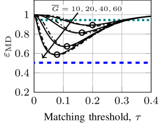
(a)

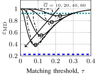
(b)

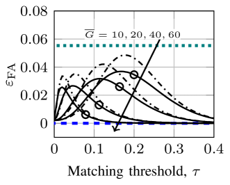
(c)

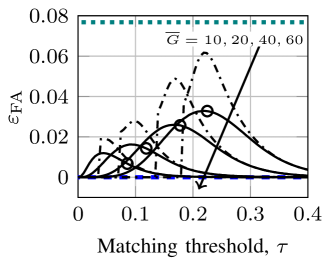
(d)

Figure 4: Probability of MD (4(a)-4(b)) and FA (4(c)-4(d)) vs. matching threshold $\tau$ for ALOHA and IRSA under the Gaussian observation model. The solid lines show simulation results while the dash-dotted lines show the analytical approximation, and the circles indicate the optimized thresholds obtained using the proposed procedure. The green dotted and the blue dashed lines indicate the optimal performance under traditional (query-free) random access and under perfect matching (i.e., no MD/FA), respectively.

The probability of FA is shown in Figs. 4(c) and 4(d). As for MD, a large discriminant gain generally results in a lower FA probability. While the difference in the FA probability between ALOHA and IRSA is smaller than for MD, the curves for IRSA peak lower than those of ALOHA. This is because ALOHA performs better than IRSA for high frame loads (i.e., low thresholds), where the fraction of FA transmissions is large. On the other hand, IRSA supports a much higher throughput than ALOHA at moderate frame loads, where the fraction of FA is lower. Finally, the figure shows that the analytical approximation deviates significantly from the simulated results. However, this is primarily due to the low probability of FA, since the absolute error is similar to the one in Figs. 4(a) and 4(b), and the approximation still characterizes the main trend of the FA probabilities. In all cases, the proposed semantic data sourcing method significantly reduces false alarms compared to what can be achieved with traditional random access, as indicated by the green dotted line.

Fig. 5 shows the MD and FA probabilities vs. the query dimension using the optimized thresholds. As expected, a larger dimension decreases both the probability of MD and of FA. The MD probability for IRSA (dashed line) is generally lower than for ALOHA (solid line), especially at high query dimensions. This suggests that the increased throughput of IRSA makes it possible to take better advantage of the increased discernibility that comes with a higher query dimension. In the case of FA, IRSA is generally better than ALOHA at low query dimensions and similar to ALOHA at high dimensions.

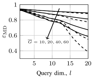
(a)

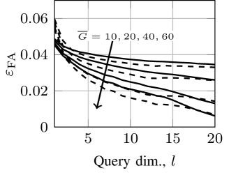
(b)

Figure 5: Probability of MD (5(a)) and FA (5(b)) vs. query dimension $l$ under the Gaussian observation model and using optimized thresholds for ALOHA (solid) and IRSA (dashed).

Finally, we consider the end-to-end inference accuracy vs. the matching threshold in Fig. 6. As expected, a larger discriminant gain results in higher accuracy. Furthermore, the optimized threshold approximately maximizes the accuracy, confirming that the number of received true positives serves as a good proxy for inference accuracy. However, despite the fact that the protocol with IRSA has a much smaller probability of MD (see Figs. 4(a) and 4(b)), the inference accuracy achieved by IRSA and ALOHA is similar. This suggests that only a small number of true positives are sufficient to perform accurate inference in the specific task. Furthermore, for low discriminant gains the inference errors are dominated by “noisy” query examples and resulting FA observations, which cannot be compensated by the higher transmission success probability offered by IRSA.

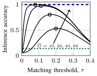
(a)

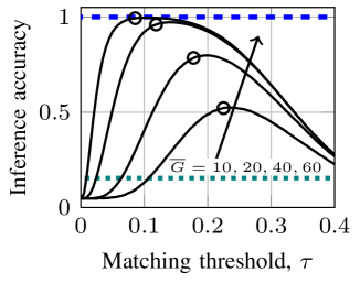
(b)

Figure 6: Inference accuracy vs. matching threshold $\tau$ for (6(a)) ALOHA and (6(b)) IRSA under the Gaussian observation model. The line styles are the same as in Fig. 4.

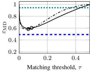
(a)

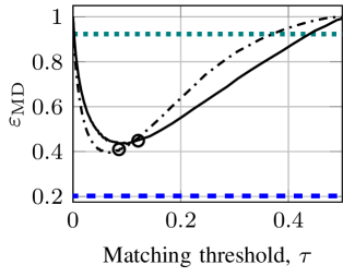
(b)

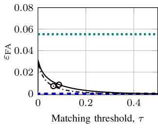
(c)

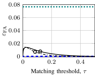
(d)

Figure 7: Probability of MD (7(a)-7(b)) and FA (7(c)-7(d)) vs. matching threshold $\tau$ for ALOHA and IRSA under the CNN classification model with $l=8$ (solid) and $l=64$ (dash-dotted). The green dotted and the blue dashed lines indicate the optimal performance under traditional (query-free) random access and under perfect matching, respectively.

VI-B CNN Classification

To study a more realistic scenario, we next consider CNN-based semantic data sourcing presented in Section V. The input images are drawn from the multi-view ModelNet40 dataset [33] following the model outlined in Section II-A2. We use the feature extraction layers of the VGG11 model [34] as the observation feature encoder $f_{\mathrm{enc}}(\cdot)$, which results in $d=25088$ features. The query and key encoders $f_{\mathrm{q}}(\cdot)$ and $f_{\mathrm{k}}(\cdot)$ are both feed-forward neural networks comprising a single hidden layer with 1024 neurons and ReLU activations. The classifier $f_{\mathrm{ser}}(\cdot)$ is constructed using the classifier layers of the VGG11 model to predict the $|\mathcal{Z}|=40$ categories in the ModelNet40 dataset. Both the VGG11 feature extraction layers and the classifier layers are pre-trained on the ImageNet dataset, and then fine-tuned along with the query and key encoder networks on the ModelNet40 dataset with the cross-entropy loss function. Specifically, we split the ModelNet40 training dataset into three disjoint subsets: 80% of the samples are used for training the CNN, 10% for validation, and 10% for calibration (matching threshold optimization). Each of the ModelNet40 subsets are then used to construct samples following the model in Section II-A2. Unless specified, other system parameters are the same as in the GMM experiments.

Fig. 7 shows the probability of MD and FA vs. the matching threshold for query sizes $l=8$ (solid) and $l=64$ (dash-dotted). Similar to the Gaussian case, the MD first decreases with the threshold $\tau$ and then increases, whereas the FA first increases and then decreases. Furthermore, as expected the query dimension $l=64$ generally results in a lower probability of both MD and FA compared to $l=8$, and IRSA performs better than ALOHA. Note that there is a significant gap between the achieved MD/FA and the optimal performance under perfect matching (dashed blue line), suggesting, as in the GMM scenario, that noisy queries and FA significantly impact the performance. However, compared to traditional random access (green dotted line), semantic data sourcing leads to a significant reduction in both MD and FA.

Finally, Fig. 8 shows the resulting accuracy. As for the GMM, IRSA does not provide significantly higher accuracy compared to ALOHA despite having lower probability of MD and FA, suggesting that bad query examples are the main limitation for accuracy. Overall, the insights obtained from the GMM accurately captures the main behavior of the much more complex CNN, suggesting that the GMM is a good proxy for studying the semantic query-based retrieval problem.

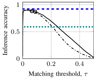
(a)

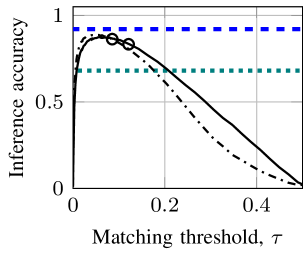
(b)

Figure 8: Inference accuracy vs. matching threshold $\tau$ for (8(a)) ALOHA and (8(b)) IRSA under the CNN classification model. The line styles are the same as in Fig. 7.

VII Conclusion

Effective retrieval of sensing data represents a challenge in massive IoT networks. This paper introduces an efficient pull-based data collection protocol for this scenario, termed semantic data sourcing random access. The protocol utilizes semantic queries transmitted by the destination node to enable devices to assess the importance of their sensing data, and relies on modern random access protocols for efficient transmission of the relevant observations. We analyze and explore the tradeoff between MD, FA, and collisions in the random access phase under a tractable GMM, and optimize the matching score threshold to minimize the probability of MD. We also show how the framework can be applied to more realistic but complex scenarios based on a CNN-based model for visual sensing data. Through numerical results, we show that the threshold selection method achieves near-optimal performance in terms of the probability of MD and FA, and that the analysis of the GMM is consistent with results observed from the CNN-based model. Furthermore, the proposed protocol significantly increases the fraction of relevant retrieved observations compared to traditional random access methods, highlighting the effectiveness of semantic query-based data sourcing random access for massive IoT. Future directions include multi-round, feedback-enhanced semantic queries, and energy-efficient semantic queries using, e.g., wake-up radios.

Appendix A Proof of Lemma 1

We first derive the probability of FA, $\varepsilon_{\mathrm{FA},\mathrm{match}}(\tau)$, which occurs if the matching score exceeds $\tau$ when the device observation class $z_{m}$ is distinct from the query class $z_{q}$. Let $S_{m}$ denote the event that device $m$ successfully decodes the query transmission, so that $\Pr(S_{m})=1-p_{\mathrm{err},m}^{\mathrm{dl}}$. Since a successful query transmission is required to perform matching, the probability of FA can be expressed as

$$\varepsilon_{\mathrm{FA},\mathrm{match}}(\tau) =(1-p_{\mathrm{err}}^{\mathrm{dl}})\Pr(\mathrm{FA}|S_{m},\tau),$$ (28)

where $\Pr(\mathrm{FA}|S_{m},\tau)$ is the probability of FA given successful query reception. This probability is

$$\Pr(\mathrm{FA}|S_{m},\tau)=\Pr(\bar{\chi}(\bm{x}_{m},\bm{q})\geq\tau|z_{m}\neq z_{q})$$

$$\quad\!=\!\frac{2\sum_{i=1}^{|\mathcal{Z}|}\sum_{j=i+1}^{|\mathcal{Z}|}\Pr(\|\bm{k}_{m}-\bm{q}\|_{2}^{2}\leq\tilde{\tau}|z_{m}=i,z_{q}=j)}{|\mathcal{Z}|(|\mathcal{Z}|-1)},$$ (29)

where the last step follows from the uniform distribution of $z_{m}$ and $z_{q}$, the monotonicity of $\bar{\chi}(\bm{x}_{m},\bm{q})$ in $\|\bm{k}_{m}-\bm{q}\|_{2}^{2}$, and substituting $\tilde{\tau}=d\ln(1/\tau)$.

Given the expressions in Eqs. 12 and 13 the query and key vectors $\bm{q}$ and $\bm{k}_{m}$ are both independent multivariate Gaussian random variables conditioned on $z_{q}$ and $z_{m}$ with mean $(\sqrt{d/l})\mathbf{P}_{l}\bm{\Sigma}^{-\frac{1}{2}}\bm{\mu}_{z_{q}}$ and $(\sqrt{d/l})\mathbf{P}_{l}\bm{\Sigma}^{-\frac{1}{2}}\bm{\mu}_{z_{m}}$, respectively, and covariance matrix $(d/l)\mathbf{P}_{l}\mathbf{P}_{l}^{T}=(d/l)\mathbf{I}_{l}$. Thus $\frac{l}{2d}\|\bm{k}_{m}-\bm{q}\|_{2}^{2}$ follows a noncentral chi-square distribution with $l$ degrees of freedom and noncentrality parameter

$$\textstyle\sum_{n=1}^{l}\left(\left[\left(\sqrt{1/2}\right)\mathbf{P}_{l}\bm{\Sigma}^{-\frac{1}{2}}\left(\bm{\mu}_{z_{m}}-\bm{\mu}_{z_{q}}\right)\right]_{n}\right)^{2}$$

$$\qquad=\frac{1}{2}\left(\bm{\mu}_{z_{m}}-\bm{\mu}_{z_{q}}\right)^{T}\bm{\Sigma}^{-\frac{1}{2}}\mathbf{P}_{l}^{T}\mathbf{P}_{l}\bm{\Sigma}^{-\frac{1}{2}}\left(\bm{\mu}_{z_{m}}-\bm{\mu}_{z_{q}}\right)$$

$$\qquad\triangleq G_{z_{m},z_{q}}(\mathbf{P}_{l})/2.$$

Using the expression for the cumulative density function (CDF) of a noncentral chi-square distribution, we obtain

$$\Pr\left(\|\bm{k}_{m}-\bm{q}\|_{2}^{2}\leq\tilde{\tau}l/(2d)\,\middle|\,z_{m}=i,z_{q}=j\right)$$

$$\qquad=1-Q_{\frac{l}{2}}\left(\sqrt{G_{i,j}(\mathbf{P}_{l})/2},\sqrt{\tilde{\tau}l/(2d)}\right)$$

$$\qquad=1-Q_{\frac{l}{2}}\left(\sqrt{G_{i,j}(\mathbf{P}_{l})/2},\sqrt{(l/2)\ln(1/\tau)}\right).$$ (30)

The final expression for $\varepsilon_{\mathrm{FA},\mathrm{match}}(\tau)$ follows by defining $\tilde{\tau}=l\ln(1/\tau)$ and combining Eqs. 28, 29 and 30.

The derivation of the probability of MD, $\varepsilon_{\mathrm{MD},\mathrm{match}}(\tau)$, is similar. A MD occurs whenever a device observation from the query class is not transmitted, either due to downlink communication error or an unsuccessful semantic matching. The probability can be expressed as

$$\varepsilon_{\mathrm{MD},\mathrm{match}}(\tau) =1-\left(1-p_{\mathrm{err}}^{\mathrm{dl}}\right)\left(1-\Pr(\mathrm{MD}|S_{m},\tau)\right),$$ (31)

where $\Pr(\mathrm{MD}|S_{m},\tau)$ is the probability of MD given successful query reception. This probability is

$$\Pr(\mathrm{MD}|S_{m},\tau) =\Pr(\bar{\chi}(\bm{k}_{m},\bm{q})\leq\tau|z_{m}=z_{q})$$

$$=\Pr(\|\bm{k}_{m}-\bm{q}\|_{2}^{2}\geq\tilde{\tau}|z_{m}=z_{q}).$$ (32)

Following the same argument as before, $\frac{l}{2d}\|\bm{k}_{m}-\bm{q}\|_{2}^{2}$ follows a (central) chi-square distribution with $l$ degrees of freedom. From this we obtain

$$\Pr\left(\|\bm{k}_{m}-\bm{q}\|_{2}^{2}\geq\tilde{\tau}l/(2d)\right)=\frac{\Gamma\left(l/2,(l/4)\ln(1/\tau)\right)}{\Gamma\left(l/2\right)}.$$ (33)

The final expression for $\varepsilon_{\mathrm{MD},\mathrm{match}}(\tau)$ follows by combining Eqs. 31, 32 and 33.

Appendix B Proof of Proposition 1

We prove the result by showing that problem in (16) is equivalent to Fisher’s LDA [28], which has a well-known solution. We first rewrite the objective function in Eq. 16:

$$J(\mathbf{P}_{l}) =\textstyle\frac{2}{|\mathcal{Z}|(|\mathcal{Z}|-1)}\sum_{i=1}^{|\mathcal{Z}|}\sum_{j=i+1}^{|\mathcal{Z}|}G_{i,j}(\mathbf{P}_{l})$$

$$=\textstyle\frac{1}{2}\sum_{i=1}^{|\mathcal{Z}|}\sum_{j=1}^{|\mathcal{Z}|}\|\mathbf{P}_{l}\bm{\Sigma}^{-\frac{1}{2}}\left(\bm{\mu}_{i}-\bm{\mu}_{j}\right)\|_{2}^{2}$$

$$=\textstyle\frac{1}{2}\sum_{i=1}^{|\mathcal{Z}|}\sum_{j=1}^{|\mathcal{Z}|}\|\mathbf{P}_{l}\left(\tilde{\bm{\mu}}_{i}-\tilde{\bm{\mu}}_{j}\right)\|_{2}^{2},$$ (34)

where $\tilde{\bm{\mu}}_{i}=\bm{\Sigma}^{-\frac{1}{2}}(\bm{\mu}_{i}-\bar{\bm{\mu}})$ and $\bar{\bm{\mu}}=\frac{1}{|\mathcal{Z}|}\sum_{i=1}^{|\mathcal{Z}|}\bm{\mu}_{i}$. Equation 34 can in turn be written

$$J(\mathbf{P}_{l}) =\!\textstyle\frac{1}{2}\sum_{i=1}^{|\mathcal{Z}|}\sum_{j=1}^{|\mathcal{Z}|}\operatorname{Tr}\left(\mathbf{P}_{l}\left(\tilde{\bm{\mu}}_{i}-\tilde{\bm{\mu}}_{j}\right)\left(\tilde{\bm{\mu}}_{i}-\tilde{\bm{\mu}}_{j}\right)^{T}\mathbf{P}_{l}^{T}\right)$$

$$=\!\textstyle\frac{1}{2}\!\operatorname{Tr}\!\left(\mathbf{P}_{l}\!\left(\sum_{i=1}^{|\mathcal{Z}|}\sum_{j=1}^{|\mathcal{Z}|}\left(\tilde{\bm{\mu}}_{i}\!-\!\tilde{\bm{\mu}}_{j}\right)\left(\tilde{\bm{\mu}}_{i}\!-\!\tilde{\bm{\mu}}_{j}\right)^{T}\right)\mathbf{P}_{l}^{T}\right).$$

Next, we note that

$$\left[\textstyle\sum_{i=1}^{|\mathcal{Z}|}\sum_{j=1}^{|\mathcal{Z}|}\left(\tilde{\bm{\mu}}_{i}-\tilde{\bm{\mu}}_{j}\right)\left(\tilde{\bm{\mu}}_{i}-\tilde{\bm{\mu}}_{j}\right)^{T}\right]_{k,l}$$

$$\qquad=\textstyle\sum_{i=1}^{|\mathcal{Z}|}\sum_{j=1}^{|\mathcal{Z}|}\left(\tilde{\bm{\mu}}_{i}[k]-\tilde{\bm{\mu}}_{j}[k]\right)\left(\tilde{\bm{\mu}}_{i}[l]-\tilde{\bm{\mu}}_{j}[l]\right)^{T}$$

$$\qquad=\textstyle 2|\mathcal{Z}|\sum_{i=1}^{|\mathcal{Z}|}\left(\tilde{\bm{\mu}}_{i}[k]\tilde{\bm{\mu}}_{i}[l]-\tilde{\bm{\mu}}_{i}[l]\sum_{j=1}^{|\mathcal{Z}|}\tilde{\bm{\mu}}_{j}[l]\right)$$

$$\qquad=\textstyle 2|\mathcal{Z}|\sum_{i=1}^{|\mathcal{Z}|}\tilde{\bm{\mu}}_{i}[k]\tilde{\bm{\mu}}_{i}[l],$$

where the last step follows from the fact that $\sum_{j=1}^{|\mathcal{Z}|}\tilde{\bm{\mu}}_{j}=\sum_{j=1}^{|\mathcal{Z}|}\bm{\Sigma}^{-\frac{1}{2}}(\bm{\mu}_{i}-\bar{\bm{\mu}})=\bm{0}$. It follows that

$$\textstyle\sum_{i=1}^{|\mathcal{Z}|}\sum_{j=1}^{|\mathcal{Z}|}\left(\tilde{\bm{\mu}}_{i}-\tilde{\bm{\mu}}_{j}\right)\left(\tilde{\bm{\mu}}_{i}-\tilde{\bm{\mu}}_{j}\right)^{T}=2|\mathcal{Z}|\sum_{i=1}^{|\mathcal{Z}|}\tilde{\bm{\mu}}_{i}\tilde{\bm{\mu}}_{i}^{T},$$

and thus

$$J(\mathbf{P}_{l}) =\textstyle|\mathcal{Z}|\operatorname{Tr}\left(\mathbf{P}_{l}\left(\sum_{i=1}^{|\mathcal{Z}|}\tilde{\bm{\mu}}_{i}\tilde{\bm{\mu}}_{i}^{T}\right)\mathbf{P}_{l}^{T}\right)$$

$$=|\mathcal{Z}|\operatorname{Tr}\left(\mathbf{P}_{l}\mathbf{W}\mathbf{P}_{l}^{T}\right),$$

where $\mathbf{W}=\sum_{i=1}^{|\mathcal{Z}|}\tilde{\bm{\mu}}_{i}\tilde{\bm{\mu}}_{i}^{T}=\sum_{i=1}^{|\mathcal{Z}|}\bm{\Sigma}^{-\frac{1}{2}}(\bm{\mu}_{i}-\bar{\bm{\mu}_{i}})(\bm{\mu}_{i}-\bar{\bm{\mu}_{i}})^{T}\bm{\Sigma}^{-\frac{1}{2}}$. Disregarding the constant $|\mathcal{Z}|$, maximizing $\operatorname{Tr}\left(\mathbf{P}_{l}\mathbf{W}\mathbf{P}_{l}^{T}\right)$ with the constraint $\mathbf{P}_{l}\mathbf{P}_{l}^{T}=\mathbf{I}_{l}$ is equivalent to Fisher’s linear discriminant analysis with covariance matrix $\mathbf{I}_{d}$. This problem has the well-known solution given by

$$\mathbf{P}_{l}=\begin{bmatrix}\bm{v}_{1}^{T}&\bm{v}_{2}^{T}&\cdots&\bm{v}_{l}^{T}\end{bmatrix}^{T},$$

where $\bm{v}_{1},\bm{v}_{2},\ldots,\bm{v}_{d}\in\mathbb{R}^{d}$ are the eigenvectors of $\mathbf{W}$ ordered by the magnitude of their corresponding eigenvalues [28].

Appendix C Proof of Proposition 2

We first prove that the expression in Eq. 22 is a necessary and sufficient condition for optimality, and then show that there exists a solution for $0<\tau\leq 1$.

The derivative of Eq. 21 is

$$\frac{\mathop{}\!\mathrm{d}}{\mathop{}\!\mathrm{d}\tau}\left(\bar{\lambda}_{\mathrm{TP}}(\tau)e^{-\bar{\lambda}(\tau)/L_{\mathrm{ul}}}\right)$$

$$\quad=e^{-\bar{\lambda}(\tau)/L_{\mathrm{ul}}}{\bar{\lambda}_{\mathrm{TP}}}^{\prime}(\tau)+\bar{\lambda}_{\mathrm{TP}}(\tau)\left(\frac{\mathop{}\!\mathrm{d}}{\mathop{}\!\mathrm{d}\tau}e^{-\bar{\lambda}(\tau)/L_{\mathrm{ul}}}\right)$$

$$\quad=e^{-\bar{\lambda}(\tau)/L_{\mathrm{ul}}}{\bar{\lambda}_{\mathrm{TP}}}^{\prime}(\tau)-\frac{\bar{\lambda}_{\mathrm{TP}}(\tau)e^{-\bar{\lambda}(\tau)/L_{\mathrm{ul}}}}{L_{\mathrm{ul}}}\bar{\lambda}^{\prime}(\tau)$$

$$\quad=\!\frac{e^{-\bar{\lambda}(\tau)/L_{\mathrm{ul}}}}{L_{\mathrm{ul}}}\!\left(\!\left(L_{\mathrm{ul}}\!-\!\bar{\lambda}_{\mathrm{TP}}(\tau)\right){\bar{\lambda}_{\mathrm{TP}}}^{\prime}(\tau)\!-\!\bar{\lambda}_{\mathrm{TP}}(\tau){\bar{\lambda}_{\mathrm{FA}}}^{\prime}(\tau)\right).$$

By setting the expression equal to zero and noting that $e^{-\bar{\lambda}(\tau)/L_{\mathrm{ul}}}>0$ for $\bar{\lambda}(\tau)<\infty$, we obtain the condition

$$\psi(\tau)\overset{\triangle}{=}L_{\mathrm{ul}}-\bar{\lambda}_{\mathrm{TP}}(\tau)\left(1+\frac{{\bar{\lambda}_{\mathrm{FA}}}^{\prime}(\tau)}{{\bar{\lambda}_{\mathrm{TP}}}^{\prime}(\tau)}\right)=0.$$

To simplify the subsequent notation, let $g(\tau)=l\ln(1/\tau)$. Using the definition in Eq. 18, we have

$${\bar{\lambda}_{\mathrm{TP}}}^{\prime}(\tau) =-\frac{Mp_{\mathrm{pos}}(1-p_{\mathrm{err}}^{\mathrm{dl}})lg(\tau)^{l/2-1}}{2^{l}\Gamma(l/2)\tau^{1-l/4}},$$ (35)

where we applied the chain rule and used that $1-\Gamma(l/2,\tilde{\tau}/4)/\Gamma(l/2)$ is the CDF of a chi-squared distribution, whose derivative is the PDF. Using a similar approach with the definition in Eq. 19, but using the noncentral chi-squared distribution, we find

$${\bar{\lambda}_{\mathrm{FA}}}^{\prime}(\tau) \!=\!-\!\frac{M(1-p_{\mathrm{pos}})(1-p_{\mathrm{err}}^{\mathrm{dl}})lg(\tau)^{l/2-1}}{2|\mathcal{Z}|(|\mathcal{Z}|-1)\tau^{1-l/4}}\phi\left(g(\tau)\right)$$ (36)

where

$$\phi\left(g(\tau)\right)=g(\tau)^{1/2-l/4}\\ \textstyle\times{\sum_{i=1}^{|\mathcal{Z}|}\sum_{j=i+1}^{|\mathcal{Z}|}}\left[\frac{e^{-\frac{1}{4}G_{i,j}}}{G_{i,j}^{l/4-1/2}}I_{l/2-1}\left(\frac{1}{2}\sqrt{G_{i,j}g(\tau)}\right)\right],$$

$I_{n}(x)$ is the modified Bessel function of the first kind, and we used the shorthand $G_{i,j}$ instead of $G_{i,j}(\mathbf{P}_{l})$ for convenience. Inserting Eqs. 35 and 36 into the expression for $\psi(\tau)$ we obtain

$$\psi(\tau) =L_{\mathrm{ul}}-\bar{\lambda}_{\mathrm{TP}}(\tau)\left(1+\frac{(1-p_{\mathrm{pos}})2^{l-1}\Gamma(l/2)}{p_{\mathrm{pos}}|\mathcal{Z}|(|\mathcal{Z}|-1)}\phi\left(g(\tau)\right)\right)$$

$$=L_{\mathrm{ul}}-M(1-p_{\mathrm{err}}^{\mathrm{dl}})\gamma\left(\frac{l}{2},\frac{g(\tau)}{4}\right)$$

$$\qquad\times\left(p_{\mathrm{pos}}+\frac{(1-p_{\mathrm{pos}})2^{l-1}\Gamma(l/2)}{|\mathcal{Z}|(|\mathcal{Z}|-1)}\phi\left(g(\tau)\right)\right),$$

where the last step follows from Eqs. 18 and 14 and the identity $\Gamma(s,z)/\Gamma(s)=1-\gamma(s,z)$.

We next to show that $\psi(\tau)$ is strictly increasing in $\tau$. Since the function is continuous in the interval $0<\tau\leq 1$, strict monotonicity implies that any root of $\psi(\tau)$ (if any) is unique, and thus maximizes Eq. 21. We first note that to be strictly increasing in $\tau$ in the interval $0<\tau\leq 1$, the function must be strictly decreasing in $g(\tau)$. To this end, since all coefficients are positive it suffices to show that $\gamma(l/2,g(\tau)/4)$ and $\phi(g(\tau))$ are both strictly increasing in $g(\tau)$. Clearly, this holds for $\gamma(l/2,g(\tau)/4)$. For $\phi(g(\tau))$, it is sufficient to show that

$$g(\tau)^{1/2-l/4}I_{l/2-1}\left(\frac{1}{2}\sqrt{G_{i,j}g(\tau)}\right)$$

is increasing in $g(\tau)$ for all $i,j$. Applying the identity $I_{n}(x)=\left(\frac{x}{2}\right)^{n}\sum_{k=0}^{\infty}\frac{(x^{2}/4)^{k}}{k!\Gamma(n+k+1)}$ [35, eq. 9.6.10], we obtain

$$g(\tau)^{1/2-l/4}I_{l/2-1}\left(\frac{1}{2}\sqrt{G_{i,j}g(\tau)}\right)\\ \textstyle=2^{2-l}g(\tau)^{3(l-1)/4}G_{i,j}^{l/4-1/2}\sum_{k=0}^{\infty}\frac{(G_{i,j}g(\tau)/16)^{k}}{k!\Gamma(l/2+k)}.$$

Since this function is strictly increasing in $g(\tau)$ when $l\geq 1$ and $G_{i,j}>0$ and zero when $G_{i,j}=0$, we conclude that $\phi(g(\tau))$ is strictly increasing in $g(\tau)$, and thus $\psi(\tau)$ is strictly increasing in $\tau$ for $l\geq 1$ and $\sum_{i=1}^{|\mathcal{Z}|}\sum_{j=i+1}^{|\mathcal{Z}|}G_{i,j}>0$.

Finally, to see that $\psi(\tau)$ has a root in the interval $0<\tau\leq 1$, we note that under the conditions stated above,

$$\begin{array}[]{ll}\psi(\tau)\to-\infty,&\textrm{as }\tau\to 0,\\ \psi(\tau)\to L_{\mathrm{ul}},&\textrm{as }\tau\to 1.\end{array}$$

By the intermediate value theorem, $\psi(\tau)$ must have a root in $0<\tau<1$. Furthermore, since $\psi(\tau)$ is strictly increasing, this root is unique. The proof is completed by defining $\tilde{\tau}=g(\tau)$.

References

- [1] A. E. Kalør, P. Popovski, and K. Huang, “Random access protocols for correlated IoT traffic activated by semantic queries,” in Proc. 21st Int. Symp. Modeling Optim. Mobile, Ad Hoc Wireless Netw. (WiOpt), 2023, pp. 643–650.
- [2] M. Chiang and T. Zhang, “Fog and IoT: An overview of research opportunities,” IEEE Internet Things J., vol. 3, no. 6, pp. 854–864, 2016.
- [3] A. E. Kalør et al., “Wireless 6G connectivity for massive number of devices and critical services,” Proc. IEEE, pp. 1–23, 2024.
- [4] P. Popovski et al., “A perspective on time toward wireless 6G,” Proc. IEEE, vol. 110, no. 8, pp. 1116–1146, 2022.
- [5] M. Kountouris and N. Pappas, “Semantics-empowered communication for networked intelligent systems,” IEEE Commun. Mag., vol. 59, no. 6, pp. 96–102, 2021.
- [6] E. C. Strinati et al., “Goal-oriented and semantic communication in 6G AI-native networks: The 6G-GOALS approach,” in Proc. Joint Eur. Conf. Netw. Commun. 6G Summit (EuCNC/6G Summit), 2024, pp. 1–6.
- [7] E. Uysal et al., “Semantic communications in networked systems: A data significance perspective,” IEEE Netw., vol. 36, no. 4, pp. 233–240, 2022.
- [8] N. Rasiwasia, P. J. Moreno, and N. Vasconcelos, “Bridging the gap: Query by semantic example,” IEEE Trans. Multimedia, vol. 9, no. 5, pp. 923–938, 2007.
- [9] R. D. Yates, Y. Sun, D. R. Brown, S. K. Kaul, E. Modiano, and S. Ulukus, “Age of information: An introduction and survey,” IEEE J. Sel. Areas Commun., vol. 39, no. 5, pp. 1183–1210, 2021.
- [10] O. Ayan, M. Vilgelm, M. Klügel, S. Hirche, and W. Kellerer, “Age-of-information vs. value-of-information scheduling for cellular networked control systems,” in Proc. 10th ACM/IEEE Int. Conf. Cyber-Phys. Syst., 2019, pp. 109–117.
- [11] A. Maatouk, S. Kriouile, M. Assaad, and A. Ephremides, “The age of incorrect information: A new performance metric for status updates,” IEEE/ACM Trans. Netw., vol. 28, no. 5, pp. 2215–2228, 2020.
- [12] F. Chiariotti et al., “Query age of information: Freshness in pull-based communication,” IEEE Trans. Commun, vol. 70, no. 3, pp. 1606–1622, 2022.
- [13] Q. Lan et al., “What is semantic communication? a view on conveying meaning in the era of machine intelligence,” J. Commun. Inf. Netw., vol. 6, no. 4, pp. 336–371, 2021.
- [14] P. Agheli, N. Pappas, and M. Kountouris, “Semantic filtering and source coding in distributed wireless monitoring systems,” IEEE Trans. Commun., vol. 72, no. 6, pp. 3290–3304, 2024.
- [15] S. Kapadia and B. Krishnamachari, “Comparative analysis of push-pull query strategies for wireless sensor networks,” in Dist. Comput. Sensor Syst. Springer, 2006, pp. 185–201.
- [16] Y. Yao and J. Gehrke, “The cougar approach to in-network query processing in sensor networks,” SIGMOD Rec., vol. 31, no. 3, pp. 9–18, 2002.
- [17] J. Shiraishi, H. Yomo, K. Huang, Č. Stefanović, and P. Popovski, “Content-based wake-up for top- query in wireless sensor networks,” IEEE Trans. Green Commun. Netw., vol. 5, no. 1, pp. 362–377, 2020.
- [18] J. Shiraishi, M. Thorsager, S. R. Pandey, and P. Popovski, “TinyAirNet: TinyML model transmission for energy-efficient image retrieval from IoT devices,” IEEE Commun. Lett., vol. 28, no. 9, pp. 2101–2105, 2024.
- [19] K. Huang, Q. Lan, Z. Liu, and L. Yang, “Semantic data sourcing for 6G edge intelligence,” IEEE Commun. Mag., vol. 61, no. 12, pp. 70–76, 2023.
- [20] Z. Liu and K. Huang, “Semantic-relevance based sensor selection for edge-AI empowered sensing systems,” arXiv preprint arXiv:2503.12785, 2025.
- [21] G. Liva, “Graph-based analysis and optimization of contention resolution diversity slotted aloha,” IEEE Trans. Commun., vol. 59, no. 2, pp. 477–487, 2011.
- [22] A. Munari, “Modern random access: An age of information perspective on irregular repetition slotted ALOHA,” IEEE Trans. Commun., vol. 69, no. 6, pp. 3572–3585, 2021.
- [23] H. Su, S. Maji, E. Kalogerakis, and E. Learned-Miller, “Multi-view convolutional neural networks for 3D shape recognition,” in Proc. IEEE Int. Conf. Comput. Vision (ICCV), 2015, pp. 945–953.
- [24] A. Vaswani et al., “Attention is all you need,” in Adv. Neural Inf. Process. Syst., vol. 30, 2017, pp. 5998–6008.
- [25] Y.-C. Liu, J. Tian, N. Glaser, and Z. Kira, “When2com: Multi-agent perception via communication graph grouping,” in Proc. IEEE/CVF Conf. Comput. Vision Pattern Recognit. (CVPR), 2020, pp. 4106–4115.
- [26] Y. Hu, S. Fang, Z. Lei, Y. Zhong, and S. Chen, “Where2comm: Communication-efficient collaborative perception via spatial confidence maps,” in Adv. Neural Inf. Process. Syst., vol. 35, 2022, pp. 4874–4886.
- [27] Q. Lan, Q. Zeng, P. Popovski, D. Gündüz, and K. Huang, “Progressive feature transmission for split classification at the wireless edge,” IEEE Trans. Wireless Commun., vol. 22, no. 6, pp. 3837–3852, 2023.
- [28] C. M. Bishop, Pattern recognition and machine learning. Springer, 2006.
- [29] M. Ivanov, F. Brännström, A. Graell i Amat, and P. Popovski, “Broadcast coded slotted aloha: A finite frame length analysis,” IEEE Trans. Commun., vol. 65, no. 2, pp. 651–662, 2017.
- [30] A. Graell i Amat and G. Liva, “Finite-length analysis of irregular repetition slotted aloha in the waterfall region,” IEEE Commun. Lett., vol. 22, no. 5, pp. 886–889, 2018.
- [31] K.-H. Ngo, G. Durisi, and A. G. i Amat, “Age of information in prioritized random access,” in proc. 55th Asilomar Conf. Signals, Syst. Comput., 2021, pp. 1502–1506.
- [32] K. Zhang, Z. Yang, and T. Başar, “Multi-agent reinforcement learning: A selective overview of theories and algorithms,” in Handbook of Reinforcement Learning and Control. Springer International Publishing, 2021, pp. 321–384.
- [33] Z. Wu, S. Song, A. Khosla, F. Yu, L. Zhang, X. Tang, and J. Xiao, “3d shapenets: A deep representation for volumetric shapes,” in Proc. IEEE/CVF Conf. Comput. Vision Pattern Recognit. (CVPR), 2015, pp. 1912–1920.
- [34] K. Simonyan and A. Zisserman, “Very deep convolutional networks for large-scale image recognition,” in Int. Conf. Learn. Repr. (ICLR), 2015.
- [35] M. Abramowitz and I. A. Stegun, Handbook of mathematical functions with formulas, graphs, and mathematical tables. New York, NY, USA: Dover, 1970.