Higher-order Exceptional Points Induced by Non-Markovian Environments

Abstract

Exceptional points (EPs) have consistently held a central role in non-Hermitian physics due to their unique physical properties and potential applications. They have been intensively explored in parity-time ($\mathcal{P}\mathcal{T}$)-symmetric systems or other non-Hermitian systems; however, they barely investigated in pseudo-Hermitian systems with non-Markovian environments. In this work, we study higher-order EPs in three coupled cavities (denoted as $a$, $b_{1}$, and $b_{2}$) under pseudo-Hermitian conditions. Specifically, the cavity $a$ simultaneously interacts with two Markovian environments, while the cavity $b_{1}$ and $b_{2}$ couples with the respective Markovian environments. Through coherent perfect absorption (CPA) of two input fields with the cavity $a$, we obtain an effective gain for the system. Under certain parametric conditions, the effective Hamiltonian of the system holds pseudo-Hermiticity, where the third-order exceptional point (EP3) can be observed by measuring the output spectrum of the system. Moreover, we generalize the results to the non-Markovian regimes (only two environments coupling with the cavity $a$ are non-Markovian, while the other two environments coupling with cavities $b_{1}$ and $b_{2}$ are Markovian), which leads to the emergence of fourth-order exceptional points (EP4) and fifth-order exceptional points (EP5). In particular, EP4 and EP5 in the non-Markovian limit (corresponding to the infinite spectral width) can return to EP3 under the Markovian approximation. Finally, we extend the systems to more general non-Hermitian ones without pseudo-Hermitian constraints and find the higher-order EPs (EP6 and EP7), where all four environments are non-Markovian. The study presents expansions of non-Hermitian physics into the field of non-Markovian dynamics and anticipates the profound impact in quantum optics and precision measurement.

I Introduction

Quantum information processing and the investigation of unique physical phenomena have found a promising avenue in superconducting (SC) circuits as evidenced by extensive reviews Xiang6232013 ; Schoelkopf6642008 ; Kurizki8662015 . Quijandría and colleagues introduced the concept of parity-time ($\mathcal{P}\mathcal{T}$)-symmetric phase transition occurring at the exceptional point (EP) within the framework of SC circuits 8462018 , while Dogra et al. Subsequently, this phenomenon was replicated by applying IBM’s SC quantum computing platform Dogra262021 . Experimental observations have further strengthened these theoretical findings with EP signatures being detected in dissipative SC qubits Naghiloo2322019 ; Chen5042021 ; Chen4022022 ; Wang3092021 and interconnected systems comprising two dissipative SC resonators Partanen5052019 . Moreover, Han and his team have experimentally demonstrated the exceptional entanglement transition in the nearby area to EP Han2012023 alongside the topological invariant associated with EP3 Han02839 through meticulous monitoring of the dynamical behavior within SC circuits. Recently, Zhang et al. have studied the higher-order exceptional surface in SC circuit Zhang06062 .

Over the past decades, the remarkable focus has been gained by exceptional points (EPs) Feng7522017 ; Ganainy112018 ; Ozdemir7832019 ; Wiersig0052021 ; Bergholtz0052021 . Specifically, the $k$th-order exceptional point (EP$k$, where $k$ is greater than or equal to 2) denotes the spectral anomaly observed in non-Hermitian Hamiltonians characterized by the convergence of both $k$ eigenvalues and their corresponding eigenstates Heiss0162012 ; Schnabel053868 ; Pan011601 ; Chakraborty063846 ; Laha063829 ; Ramezanpour043510 ; Yazdi052230 ; Yu144414 ; Mandal186601 . At the degeneracy of Hermitian Hamiltonians, the eigenvalues coalesce and the associated eigenvectors maintain orthogonality. The spectral anomaly surrounding EPs can induce a multitude of fascinating phenomena, containing unidirectional invisibility Lin9012011 ; Cheng-invisibility2025 ; Peng3942014 , resilient wireless energy transmission 3872017 ; Hao2022023 , asymmetric modal transitions Doppler762016 ; Xu802016 , augmented spontaneous radiation Lin4022016 , unidirectional lasing Longhi2017 , exotic topological states Zhou0092018 ; Yang0132018 , sensitivity enhancement Hodaei1872017 ; Zheng2019 ; Xie2024 ; Guo2024 ; Bowang-PT2025 ; Wiersig9012014 ; Chen1922017 ; Zhang3072021 ; Liu8022016 , laser mode selection Feng9722014 ; Hodaei9752014 , coherent perfect absorption Sun9032014 ; Zhang3682017 ; Wang2612021 , electromagnetically induced transparency Wang3342020 ; Wang0692019 , and speeding up entanglement generation Li2022023 . These exceptional points manifest complex topological characteristics in interconnected acoustic resonators Ding0072016 .

A necessary condition for a closed quantum system’s Hamiltonian yielding a real energy spectrum is its Hermiticity. However, practical quantum systems always operate as open systems. Under specific circumstances, these systems can be represented by non-Hermitian Hamiltonians. Mostafazadeh introduced the concept of pseudo-Hermiticity for such Hamiltonians Mostafazadeh2052002 ; Mostafazadeh22002 ; Mostafazadeh32002 , where a Hamiltonian $\hat{H}$ with a discrete energy spectrum is deemed pseudo-Hermitian if it satisfies the relation $\hat{H}^{\dagger}=\hat{U}\hat{H}\hat{U}^{-1}$ with $\hat{U}$ being a linear Hermitian operator. The corresponding eigenvalues are confined to being either purely real or occurring in complex-conjugate pairs. The topic of pseudo-Hermiticity unlocks a universe of intriguing phenomena spanning various physics domains containing quantum chaos, quantum phase transitions Deguchi1072009 ; Deguchi2132009 ; Shen0121072016 , Dirac particles navigating gravitational fields Gorbatenko0562010 , Maxwell’s equations in novel contexts Zhu9052011 , the anisotropic XY model Zhang1142013 , and dynamical invariants Simeonov1232016 .

The field of $\mathcal{P}\mathcal{T}$-symmetric Hamiltonians constitutes another segment within the pseudo-Hermitian landscape characterized by the condition $[H,\mathcal{P}\mathcal{T}]=0$ with $\mathcal{P}$ and $\mathcal{T}$ respectively being the parity and time operators Mostafazadeh32002 ; Konotop0022016 . As a system’s parameters approach a critical moment (known as EP) a quantum phase transition unfolds, transforming the system from a $\mathcal{P}\mathcal{T}$-symmetric phase to a $\mathcal{P}\mathcal{T}$-symmetry-breaking phase in the parameter space. This transition is marked by a shift from real to complex eigenvalues Konotop0022016 , where the EP itself is also referred to as the second-order exceptional point (EP2), which is a topic of extensive investigation through various non-Hermitian systems, containing optomechanical setups L¨¹6012015 ; Xu802016 , coupled waveguides Doppler762016 ; Paul063503 ; Dey126644 ; Li0237122024 , optical microresonator networks Chang5242014 , cavity magnonics systems Harder4112017 ; Gao8262017 ; Wang2482018 , and superconducting circuit-QED configurations 8462018 . However, the constraint of $\mathcal{P}\mathcal{T}$ symmetry acts as a strict limitation on the system’s parameters, especially in attempting to engineer EPs of higher orders. The subsequent discussions on pseudo-Hermiticity shall exclude both the aforementioned Hermiticity and $\mathcal{P}\mathcal{T}$ symmetry, paving the way for a more comprehensive exploration of non-Hermitian phenomena. In the field of pseudo-Hermitian physics devoid of $\mathcal{P}\mathcal{T}$ symmetry, higher-order EPs and their relevant applications have been extensively explored through various physical systems, containing cavity-magnon systems Zhang4042019 ; Zhang4172023 ; Hu01613 , cavity optomechanical systems Xiong5082021 ; Xiong5182022 ; Zhang2400275 , radio-frequency circuits Yin0032023 , and atom-cavity QED systems Li3722023 .

The rapid progress in quantum information technology advancements nielsen2000 ; Ladd452010 has spotlighted open quantum systems BreuerOxford2002 ; WeissSingapore2008 , drawing heightened interest. In general, every quantum system encountered in nature is open due to the unavoidable entanglement with its surrounding environment Lu_higher_2023 ; GardinerBerlin2000 ; Shang_sym_2023 ; Li0621242010 ; Franco13450532013 ; Shang_entanglement2024 ; Caruso12032014 ; Shang-nonreciprocity2019 ; dissipativeHC_2025 . The Markovian approximation for open systems BreuerOxford2002 ; WeissSingapore2008 is valid only under conditions of weak system-environment coupling and the system’s characteristic timescales significantly exceeding those of the environmental bath. In contrast, cases necessitating consideration of non-Markovian dynamics NH_gain2025 ; USP-NM2018 ; Reuther0621232012 ; Luan-router2025 , arising in various quantum setups like interconnected cavities Link0203482022 , photonic crystals Burgess0622072022 ; hoeppe1080436032012 , colored noise environments CostaFilho0521262017 , cavity-waveguide hybrids Chang0521052010 ; Longhi0638262006 ; Sounas2017 ; Vega0150012017 ; LuTQB2025 ; Shen0437142024 ; Zhang0337012024 , exceptional pointsLin18362 ; Zhang06977v1 ; Wilkey1299 ; Mouloudakis053709 ; Garmon033029 ; Yang053712 , and experimental implementations Liu20117 ; Xiong2019100 ; Cialdi2019100 ; Khurana201999 ; Madsen2011106 ; Guo2021126 ; Li2022129 ; Xu201082 ; Tang201297 ; Uriri2020101 ; Anderson199347 ; Liu2020102 ; Groblacher76062015 , emphasize the importance of these effects. The non-Markovian processes have proven crucial in quantum information tasks, containing state engineering, control, and enhancing channel capacities bylicka457202014 ; Shen0321012019 ; Xin0537062022 ; xue860523042012 . The appearance of non-Markovianity (as the environments have influences on system dynamics that reaches back and affects previous states) is illustrated by the repeated exchange of excitations between the system and its surrounding environments breuer880210022016 ; breuer1032104012009 ; laine810621152010 ; addis900521032014 ; wibmann860621082012 ; wibmann920421082015 ; Shen7072022 . This creates the foundation for various methods of measuring non-Markovian regimes lorenzo880201022013 ; rivas1050504032010 ; luo860441012012 ; wolf1011504022008 ; lu820421032010 ; chruscinski1121204042014 .

In this work, we investigate the high-order EPs in three coupled cavities [see Fig. 1]. When the system parameters satisfy certain constraints, the Hamiltonian of the system exhibits pseudo-Hermiticity, which can be obtained through coherent perfect absorption (CPA) of the two input fields fed into the cavity via two ports. Under the Markovian approximation, the EP3 Li03768 ; Kim2023 ; Bhattacherjee2019 ; Kullig2018 ; Yan2023 ; Jing3386 ; Habler2020 ; Sahoo2022 ; Novitsky2022 ; Montag2024 ; Zhang2023 corresponding to the effective Hamiltonian can be obtained. When the two input fields of the cavity $a$ are placed under identical or different non-Markovian environments, the corresponding Hamiltonian exhibits characteristics of EP4 CrippaL121109 ; Bhattacherjee062124 ; Jin012121 ; Othman104305 ; Dey07903 ; Qin10001 ; Arkhipov012205 ; Wu6080 ; Zhou10118 ; Shen065102 ; Kaltsas4447 ; Zhang2020 and EP5 Bai266901 ; Pan063616 ; Zhang033820 , respectively. Moreover, we study the energy spectrum and output spectrum of the pseudo-Hermitian system near these EPs. We explore the energy spectrum structure of high-order EPs including EP4 and EP5 in more general non-Hermitian systems (i.e., non-pseudo-Hermitian cases) with non-Markovian environments. Based on this, we consider the emergence of EP6 Xiao213901 ; Nada2319 ; Kullig2023 and EP7 when the cavities $b_{1}$ and $b_{2}$ are respectively placed in identical and different non-Markovian environments which lays a solid groundwork for exploring EPs and their potential applications in superconducting circuits Zhong1539022019 ; Qin20005692021 ; Li0335052021 ; Carlo59542021 ; Carlo60212022 ; Jiang2011062023 ; Zhong0132202021 ; Zhong52422019 ; Soleymani5992022 ; Tang66602023 ; Jia2932023 ; Stalhammar2011042021 ; Chen0315012022 ; Zhong0140702020 .

The remainder of this paper is organized as follows. In Sec. II, we introduce the three coupled cavities system and obtain the pseudo-Hermitian conditions. In Sec. III, we investigate the EP3 of the system under the Markovian approximation. In Sec. IV, we derive the input-output relation and pseudo-Hermitian conditions for the system with non-Markovian environments. In Sec. V, we study the EP4 of the system in non-Markovian regimes. In Sec. VI, we investigate the EP5 of the system within the non-Markovian effects. In Sec. VII, we extend the result to more general non-Hermitian systems without pseudo-Hermitian conditions. In Sec. VIII, we discuss EP6 and EP7 in general non-Hermitian systems with non-Markovian environments. Finally, in Sec. IX, we summarize the results and conclude the paper.

II THE MODEL and effective Hamiltonian

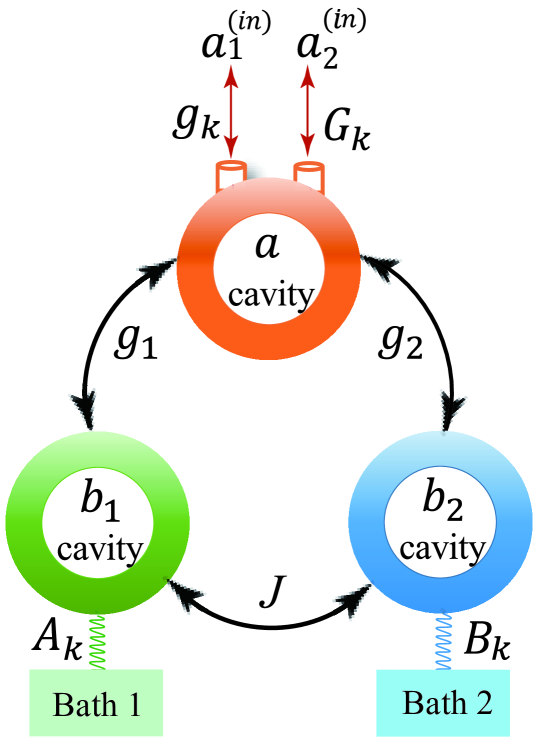
Figure 1: A schematic diagram of three coupled cavities is presented, which may be realized in superconducting circuits Zhong1539022019 ; Qin20005692021 ; Li0335052021 ; Carlo59542021 ; Carlo60212022 ; Jiang2011062023 ; Zhong0132202021 ; Zhong52422019 ; Soleymani5992022 ; Tang66602023 ; Jia2932023 ; Stalhammar2011042021 ; Chen0315012022 ; Zhong0140702020 . The cavities are characterized by the annihilation operators $\hat{a}$, $\hat{b}_{1}$, and $\hat{b}_{2}$. $g_{j}$ ($j=1,2$) and $J$ are the coupling strengths between the cavities $a$ and $b_{j}$ as well as cavities $b_{1}$ and $b_{2}$ respectively. The cavities ${b}_{1}$ and ${b}_{2}$ are coupled to their respective non-Markovian environments with strengths $A_{k}$ and $B_{k}$. Moreover, the input fields ${a}_{1}^{(in)}$ and ${a}_{2}^{(in)}$ enter the microwave cavity through ports 1 and 2 in a non-Markovian manner with coupling strengths $g_{k}$ and $G_{k}$.

Three connected cavities (marked as $a$, $b_{1}$, and $b_{2}$) together constitute the system presented in Fig. 1 with the Hamiltonian (setting $\hbar\equiv 1$)

$$\hat{H}= \ \omega_{c}\hat{a}^{\dagger}\hat{a}+\omega_{1}\hat{b}_{1}^{\dagger}\hat{b}_{1}+\omega_{2}\hat{b}_{2}^{\dagger}\hat{b}_{2}+g_{1}(\hat{a}^{\dagger}\hat{b}_{1}+\hat{a}\hat{b}_{1}^{\dagger})$$ (1)

$$+g_{2}(\hat{a}^{\dagger}\hat{b}_{2}+\hat{a}\hat{b}_{2}^{\dagger})+J(\hat{b}_{1}^{\dagger}\hat{b}_{2}+\hat{b}_{1}\hat{b}_{2}^{\dagger}),$$

where $\hat{a}$ and $\hat{a}^{\dagger}$ respectively denote the annihilation and creation operators for the cavity $a$ (with eigenfrequency $\omega_{c}$), while $\hat{b_{j}}$ and $\hat{b}_{j}^{\dagger}$ (for $j=1,2$) represent the corresponding annihilation and creation operators for the cavity $b_{j}$ (with eigenfrequency $\omega_{j}$). The coupling strength between the cavity $a$ and the cavity $b_{j}$ is given by $g_{j}$, while $J$ represents the coupling strength between the cavities $b_{1}$ and $b_{2}$. The first three terms in Eq. (1) describe the free Hamiltonian, while the last three terms constitute the interaction parts. Moreover, two input fields ${a}_{1}^{(in)}$ and ${a}_{2}^{(in)}$ are fed into the cavity $a$ through ports 1 and 2 in two non-Markovian environments with coupling strengths $g_{k}$ and $G_{k}$. The cavities $b_{1}$ and $b_{2}$ are coupled to their respective non-Markovian environments with strengths $A_{k}$ and $B_{k}$. In Sec. II- Sec. III, we focus on the Markovian case with EP3, while the remaining part of the paper explores the influences of non-Markovian effects on higher-order exceptional points changing from EP4 to EP7.

Under the Markovian approximation, the Heisenberg-Langevin equations with Eq. (1) are given by GardinerBerlin2000

$$\frac{d}{dt}\hat{a}= -i[\omega_{c}-i(\kappa_{1}+\kappa_{2})]\hat{a}-ig_{1}\hat{b}_{1}-ig_{2}\hat{b}_{2}$$

$$+\sqrt{2\kappa_{1}}\hat{a}_{1}^{(in)}+\sqrt{2\kappa_{2}}\hat{a}_{2}^{(in)},$$

$$\frac{d}{dt}\hat{b}_{1}= -i(\omega_{1}-i\gamma_{1})\hat{b}_{1}-ig_{1}\hat{a}-iJ\hat{b}_{2},$$ (2)

$$\frac{d}{dt}\hat{b}_{2}= -i(\omega_{2}-i\gamma_{2})\hat{b}_{2}-ig_{2}\hat{a}-iJ\hat{b}_{1},$$

where $\kappa_{\nu}$ represents the decay rate of the cavity $a$ attributed to the $\nu$th port ($\nu=1,2$) and is dynamically tuned Zhang3682017 . The combined decay rate for the cavity $a$ is given by $\kappa_{1}+\kappa_{2}$. If the cavity $b_{j}$ is passive (active), the loss rate (gain rate) is positive (negative), i.e., $\gamma_{j}>0$ $(\gamma_{j}<0)$, while no external input field is applied to the cavity $b_{j}$. Here, $\gamma_{j}$ represents the dissipation, which is introduced phenomenologically. We assume that the coupling strength $g_{j}$ and $J$ are non-negative, while the cavity $b_{1}$ and $b_{2}$ are lossy.

Based on the Markovian input-output theory, a relationship can be established by linking the intracavity field $a$ with both the input field $\hat{a}_{\nu}^{(in)}$ and output field $\hat{a}_{\nu}^{(out)}$ though

$$\hat{a}_{\nu}^{(in)}+\hat{a}_{\nu}^{(out)}=\sqrt{2\kappa_{\nu}}\hat{a}$$ (3)

at the respective ports shown in Fig. 1.

II.1 Effective Hamiltonian under the Markovian approximation

Under suitable parameter settings, the system may exhibit CPA (as detailed in Sec. II.2) and reach zero output fields from ports 1 and 2, specifically $\hat{a}_{\nu}^{(out)}=0$. In this case, Eq. (3) is transformed into ${\hat{a}_{\nu}}^{(in)}=\sqrt{2\kappa_{\nu}}\hat{a}$, which causes Eq. (2) to become

$$\frac{d}{dt}\hat{a}= -i[\omega_{c}+i(\kappa_{1}+\kappa_{2})]\hat{a}-ig_{1}\hat{b}_{1}-ig_{2}\hat{b}_{2},$$ (4)

$$\frac{d}{dt}\hat{b}_{1}= -i(\omega_{1}-i\gamma_{1})\hat{b}_{1}-ig_{1}\hat{a}-iJ\hat{b}_{2},$$

$$\frac{d}{dt}\hat{b}_{2}= -i(\omega_{2}-i\gamma_{2})\hat{b}_{2}-ig_{2}\hat{a}-iJ\hat{b}_{1}.$$

The matrix form of the Heisenberg-Langevin equations in Eq. (4) is given by $\dot{\mathbf{V}}=-i\hat{H}_{\rm{Meff}}\mathbf{V}$, where $\mathbf{V}=(\hat{a},\hat{b}_{1},\hat{b}_{2})^{T}$ stands for a column vector, while $\hat{H}_{\rm{Meff}}$ denotes the effective non-Hermitian Hamiltonian of the system

$$\hat{H}_{\rm{Meff}}=\begin{pmatrix}\omega_{c}+i\kappa_{g}&g_{1}&g_{2}\\ g_{1}&\omega_{1}-i\gamma_{1}&J\\ g_{2}&J&\omega_{2}-i\gamma_{2}\end{pmatrix}.$$ (5)

The sum of $\kappa_{1}$ and $\kappa_{2}$ (denoted as $\kappa_{g}$ and satisfying $\kappa_{g}>0$) indicates the effective gain of the cavity achieved through CPA Zhang3682017 ; Sun9032014 .

II.2 CPA conditions under the Markovian approximation

Using the modified Laplace transformation Shen0121562017 ; Uchiyama1282009 ; Saeki1312010 ; Shen1222015

$$\eta(\omega)=\int_{0}^{\infty}e^{i\omega t}\eta(t)dt,$$ (6)

where $e^{i\omega t}\rightarrow e^{i\omega t-\epsilon t}$ with $\epsilon\rightarrow 0^{+}$ makes $\eta(\omega)$ to converge to a finite value, then $\hat{a}\left(t\right)=\frac{1}{\sqrt{2\pi}}\int_{0}^{+\infty}a\left(\omega\right)e^{-i\omega t}d\omega$ and $\hat{b}_{j}\left(t\right)=\frac{1}{\sqrt{2\pi}}\int_{0}^{+\infty}b_{j}\left(\omega\right)e^{-i\omega t}d\omega$, the Heisenberg-Langevin equations from Eq. (2) can be changed to

$$-i[(\omega_{c}-\omega)-i\kappa_{g}]{a}(\omega)-ig_{1}{b}_{1}(\omega)-ig_{2}{b}_{2}(\omega)$$ (7)

$$+\sqrt{2\kappa_{1}}{a}_{1}^{(in)}(\omega)+\sqrt{2\kappa_{1}}{a}_{2}^{(in)}(\omega)=0,$$

$$-i[(\omega_{1}-\omega)-i\gamma_{1}]{b}_{1}(\omega)-ig_{1}{a}(\omega)-iJ{b}_{2}(\omega)=0,$$

$$-i[(\omega_{2}-\omega)-i\gamma_{2}]{b}_{2}(\omega)-ig_{2}{a}(\omega)-iJ{b}_{1}(\omega)=0.$$

The intracavity field can be derived from Eq. (48) as

$${a}{(\omega)}=\frac{\sqrt{2\kappa_{1}}{a}_{1}^{(in)}(\omega)+\sqrt{2\kappa_{2}}{a}_{2}^{(in)}(\omega)}{\kappa_{g}+i(\omega_{c}-\omega)+\sigma(\omega)},$$ (8)

where

$$\sigma(\omega)= \ \frac{i{g_{1}}^{2}[(\omega_{2}-\omega)-i\gamma_{2}]+i{g_{2}}^{2}[(\omega_{1}-\omega)-i\gamma_{1}]}{J^{2}-[(\omega_{1}-\omega)-i\gamma_{1}][(\omega_{2}-\omega)-i\gamma_{2}]}$$ (9)

$$-\frac{-2ig_{1}g_{2}J}{J^{2}-[(\omega_{1}-\omega)-i\gamma_{1}][(\omega_{2}-\omega)-i\gamma_{2}]}$$

denotes the self-energy generated by two cavities $b_{1}$ and $b_{2}$.

With Eqs. (8) and (3), the output fields ${a}_{1}^{(out)}(\omega)$ and ${a}_{2}^{(out)}(\omega)$ at ports 1 and 2 can be determined

$${a}_{1}^{(out)}(\omega) =\frac{2\kappa_{1}{a}_{1}^{(in)}(\omega)+2\sqrt{\kappa_{1}\kappa_{2}}{a}_{2}^{(in)}(\omega)}{\kappa_{g}+i(\omega_{c}-\omega)+\sigma(\omega)}-{{a}_{1}}^{(in)}(\omega),$$ (10)

$${a}_{2}^{(out)}(\omega) =\frac{2\sqrt{\kappa_{1}\kappa_{2}}{a}_{1}^{(in)}(\omega)+2\kappa_{2}{a}_{2}^{(in)}(\omega)}{\kappa_{g}+i(\omega_{c}-\omega)+\sigma(\omega)}-{a}_{2}^{(in)}(\omega).$$

During CPA, both input fields are completely coupled into the cavity, resulting in ${a}_{1}^{(out)}(\omega)$ and ${a}_{2}^{(out)}(\omega)$ is equal to zero in Eq. (10). Substituting ${a}_{i}^{(out)}(\omega)=0$ into Eq. (10), we derive three conditions.

The first requirement for the input fields ${a}_{1}^{(in)}(\omega)$ and ${a}_{2}^{(in)}(\omega)$ is denoted as

$${a}_{2}^{(in)}(\omega)=\sqrt{\kappa_{2}/\kappa_{1}}{a}_{1}^{(in)}(\omega).$$ (11)

The second and third conditions relate to the system parameters and the frequency of the input fields labeled as

$$\kappa_{g}= \ \frac{g_{2}^{2}[J^{2}\gamma_{1}+\gamma_{1}^{2}\gamma_{2}+\gamma_{2}(\omega_{\mathrm{CPA}}-\omega_{1})^{2}]+g_{1}^{2}[J^{2}\gamma_{2}+\gamma_{2}^{2}\gamma_{1}+\gamma_{1}(\omega_{\mathrm{CPA}}-\omega_{2})^{2}]}{2J^{2}\gamma_{1}\gamma_{2}+\gamma_{1}^{2}\gamma_{2}+\gamma_{2}^{2}(\omega_{\mathrm{CPA}}-\omega_{1})^{2}+\gamma_{1}^{2}(\omega_{\mathrm{CPA}}-\omega_{2})^{2}+[J^{2}-\omega_{\mathrm{CPA}}^{2}+\omega_{\mathrm{CPA}}\omega_{1}+\omega_{2}(\omega_{\mathrm{CPA}}-\omega_{2})]^{2}}$$ (12)

$$+\frac{2Jg_{1}g_{2}[\gamma_{2}(\omega_{\mathrm{CPA}}-\omega_{1})+\gamma_{1}(\omega_{\mathrm{CPA}}-\omega_{2})]}{2J^{2}\gamma_{1}\gamma_{2}+\gamma_{1}^{2}\gamma_{2}^{2}+\gamma_{2}^{2}(\omega_{\mathrm{CPA}}-\omega_{1})^{2}+\gamma_{1}^{2}(\omega_{\mathrm{CPA}}-\omega_{2})^{2}+\left[J^{2}-\omega_{\mathrm{CPA}}^{2}+\omega_{\mathrm{CPA}}\omega_{1}+\omega_{2}(\omega_{\mathrm{CPA}}-\omega_{1})\right]^{2}},$$

$$\omega_{c}-\omega_{\mathrm{CPA}}= \ \frac{2Jg_{1}g_{2}[J^{2}-\omega_{\mathrm{CPA}}^{2}+\gamma_{1}\gamma_{2}+\omega_{\mathrm{CPA}}\omega_{1}+\omega_{2}(\omega_{\mathrm{CPA}}-\omega_{1})]}{2J^{2}\gamma_{1}\gamma_{2}+\gamma_{1}^{2}\gamma_{2}^{2}+\gamma_{2}^{2}(\omega_{\mathrm{CPA}}-\omega_{1})^{2}+\gamma_{1}^{2}(\omega_{\mathrm{CPA}}-\omega_{2})^{2}+[J^{2}-\omega_{\mathrm{CPA}}^{2}+\omega_{\mathrm{CPA}}\omega_{1}+\omega_{2}(\omega_{\mathrm{CPA}}-\omega_{1})]^{2}}$$

$$+\frac{{g_{2}}^{2}\left\{{\gamma_{1}}^{2}\left(\omega_{2}-\omega_{\mathrm{CPA}}\right)+\left(\omega_{\mathrm{CPA}}-\omega_{1}\right)\left[J^{2}-\omega_{\mathrm{CPA}}^{2}+\omega_{\mathrm{CPA}}\omega_{1}+\omega_{2}\left(\omega_{\mathrm{CPA}}-\omega_{1}\right)\right]\right\}}{2J^{2}\gamma_{1}\gamma_{2}+{\gamma_{1}}^{2}\gamma_{2}^{2}+{\gamma_{2}}^{2}\left(\omega_{\mathrm{CPA}}-\omega_{1}\right)^{2}+{\gamma_{1}}^{2}\left(\omega_{\mathrm{CPA}}-\omega_{2}\right)^{2}+\left[J^{2}-\omega_{\mathrm{CPA}}^{2}+\omega_{\mathrm{CPA}}\omega_{1}+\omega_{2}\left(\omega_{\mathrm{CPA}}-\omega_{1}\right)\right]^{2}}$$

$$+\frac{g_{1}^{2}\left\{\gamma_{2}^{2}\left(\omega_{1}-\omega_{\mathrm{CPA}}\right)+\left(\omega_{\mathrm{CPA}}-\omega_{2}\right)\left[J^{2}-\omega_{\mathrm{CPA}}^{2}+\omega_{\mathrm{CPA}}\omega_{1}+\omega_{2}\left(\omega_{\mathrm{CPA}}-\omega_{1}\right)\right]\right\}}{2J^{2}\gamma_{1}\gamma_{2}+\gamma_{1}^{2}\gamma_{2}^{2}+\gamma_{2}^{2}\left(\omega_{\mathrm{CPA}}-\omega_{1}\right)^{2}+\gamma_{1}^{2}\left(\omega_{\mathrm{CPA}}-\omega_{2}\right)^{2}+\left[J^{2}-\omega_{\mathrm{CPA}}^{2}+\omega_{\mathrm{CPA}}\omega_{1}+\omega_{2}\left(\omega_{\mathrm{CPA}}-\omega_{1}\right)\right]^{2}},$$

respectively, where $\omega_{\mathrm{CPA}}$ represents the frequency of the input fields when CPA occurs. Equation (11) indicates that the two input fields must possess the same phase and maintain a particular amplitude ratio $\sqrt{\kappa_{2}/\kappa_{1}}$, which can be obtained by manipulating a tunable phase shifter and a variable attenuator during the experiment Zhang3682017 .

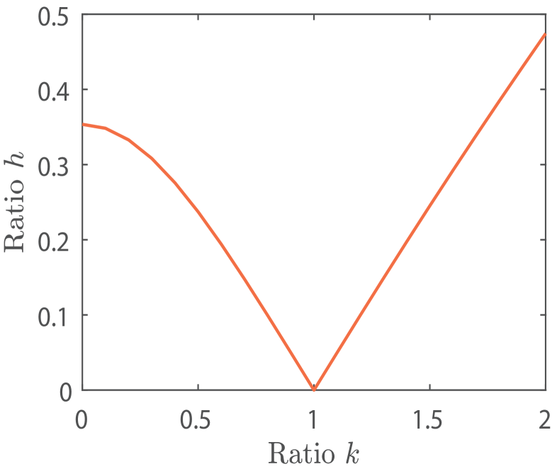
Figure 2: The ratio $h$ between the coupling strengths $J$ and $g_{1}$ varies with the ratio $k$ of the coupling strengths $g_{2}$ and $g_{1}$ under the symmetric case ($\eta=1$), which is given by Eq. (27).

II.3 Pseudo-Hermitian Hamiltonian under the Markovian approximation

In Eq. (5), we derive the necessary parameter conditions for the effective Hamiltonian $\hat{H}_{\rm{Meff}}$ to exhibit pseudo-Hermiticity, which possesses three eigenvalues. $\hat{H}_{\rm{Meff}}$ qualifies as pseudo-Hermitian only under two cases Mostafazadeh2052002 : (i) all three eigenvalues are real, or (ii) one eigenvalue is real with the remaining two forming a complex-conjugate pair. Solving the equation $\mathrm{Det}(\hat{H}_{\rm{Meff}}-\Omega I)=0$, we have

$$\begin{vmatrix}(\omega_{c}+i\kappa_{g})-\Omega&g_{1}&g_{2}\\ g_{1}&(\omega_{1}-i\gamma_{1})-\Omega&J\\ g_{2}&J&(\omega_{2}-i\gamma_{2})-\Omega\end{vmatrix}=0,$$ (13)

where $I$ denotes the identity matrix. In accordance with the energy-spectrum characteristics in Ref. Mostafazadeh2052002 for pseudo-Hermitian Hamiltonians, the complex conjugate of Eq. (13), $\mathrm{Det}(\hat{H}_{\rm{Meff}}^{*}-\Omega I)=0$, i.e.,

$$\begin{vmatrix}(\omega_{c}-i\kappa_{g})-\Omega&g_{1}&g_{2}\\ g_{1}&(\omega_{1}+i\gamma_{1})-\Omega&J\\ g_{2}&J&(\omega_{2}+i\gamma_{2})-\Omega\end{vmatrix}=0$$ (14)

should produce identical solutions.

By unfolding the factors in Eqs. (13)-(14) and matching their respective coefficients for comparison, the system’s parameters satisfy the constraints

$$\kappa_{g}-\gamma_{1}-\gamma_{2}= \ 0,$$ (15)

$$\delta_{1}\gamma_{1}+\delta_{2}\gamma_{2}= \ 0,$$

$$(\delta_{1}\delta_{2}-\gamma_{1}\gamma_{2}-J^{2})\kappa_{g}+{g_{1}}^{2}\gamma_{2}+{g_{2}}^{2}\gamma_{1}= \ 0,$$

and then the characteristic polynomial in Eq. (13) is simplifies to

$$(\Omega-\omega_{c})^{3}+c_{2}(\Omega-\omega_{c})^{2}+c_{1}(\Omega-\omega_{c})+c_{0}=0.$$ (16)

The detuning between the cavities $a$ and $b_{j}$ is expressed as $\delta_{j}=\omega_{j}-\omega_{c}$ with coefficients

$$c_{0}=g_{1}^{2}\delta_{2}+g_{2}^{2}\delta_{1}-2Jg_{1}g_{2}-\kappa_{g}\left(\gamma_{1}\delta_{2}+\gamma_{2}\delta_{1}\right),$$ (17)

$$c_{1}=\kappa_{g}^{2}+\delta_{1}\delta_{2}-\gamma_{1}\gamma_{2}-J^{2}-g_{1}^{2}-g_{2}^{2},$$

$$c_{2}=-\left(\delta_{1}+\delta_{2}\right).$$

The overall balance between loss and gain in the system is ensured by pseudo-Hermiticity, which requires $\kappa_{g}-\gamma_{1}-\gamma_{2}=0$. To simplify matters, we define three other parameters, $\eta$, $k$ and $h$, then we have

$$\gamma_{1}=\eta\gamma_{2},\>g_{2}=kg_{1},\>J=hg_{1},$$ (18)

assuming $\gamma_{2}\leqslant\gamma_{1}$ and then $\eta\geqslant 1$. Applying Eq. (18), the pseudo-Hermitian conditions in Eq. (15) become

$$\kappa_{g}= \ (1+\eta)\gamma_{2},$$ (19)

$$\delta_{2}= \ -\eta\delta_{1},$$

$$\delta_{1}^{2}= \ \frac{1+\eta k^{2}-(1+\eta)h^{2}}{(1+\eta)\eta}g_{1}^{2}-\gamma_{2}^{2},$$

while the coefficients of the characteristic polynomial in Eq. (17) result in

$$c_{0}=\left(k^{2}-\eta\right)g_{1}^{2}\delta_{1}+\left(\eta^{2}-1\right)\left(1+\eta\right)\gamma_{2}^{2}\delta_{1}-2khg_{1}^{3},$$

$$c_{1}=(1+\eta)^{2}\gamma_{2}^{2}\eta(\delta_{1}^{2}+\gamma_{2}^{2})-(1+k^{2}+h^{2})g_{1}^{2},$$

$$c_{2}=(\eta-1)\delta_{1}.$$ (20)

Drawing conclusions from the final equation in Eq. (19), we show that the coupling strength $g_{1}$ must lie within a specific range to maintain $\delta_{1}^{2}\geqslant 0$. By equating $\delta_{1}^{2}=0$, we obtain the minimal permissible value of the coupling strength $g_{1}$ (denoted as ${g}_{\mathrm{min}}$) determined by

$${g}_{\mathrm{min}}=\biggl{[}\frac{(1+\eta)\eta}{1+\eta k^{2}-(1+\eta)h^{2}}\biggr{]}^{\frac{1}{2}}\gamma_{2},$$ (21)

which is certainly feasible within the context of the system we are examining.

III Third-order exceptional points under the Markovian approximation

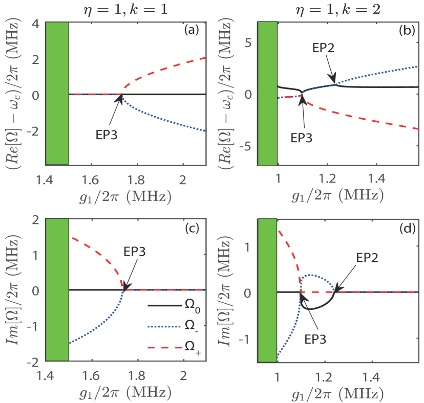
Figure 3: Under the symmetric case ($\gamma_{1}=\gamma_{2}$), the eigenvalues (both real and imaginary parts) of the effective Hamiltonian in Eq. (5) vary with the coupling strength $g_{1}$ between the cavity $a$ and the cavity $b_{1}$. The system exhibits no pseudo-Hermiticity for $g_{1}<{g}_{\text{min}}$ (represented by green regimes). In each panel, the eigenvalues $\Omega_{\pm}$ are plotted by red dashed and blue dotted lines, while the black solid line corresponds to the eigenvalue $\Omega_{0}$. (a) and (c) respectively display the real and imaginary parts of the eigenvalues $\Omega_{\pm}$ and $\Omega_{0}$ corresponding to $g_{1}$ under the symmetric condition of $\eta=k=1$. (b) and (d) denote the real and imaginary parts of the eigenvalues $\Omega_{\pm}$ and $\Omega_{0}$, corresponding to $g_{1}$ for the case with $\eta=1$ and $k=2$. The remaining parameters are set to $\kappa_{1}/2\pi=\kappa_{2}/2\pi=3$ MHz, and $\gamma_{2}/2\pi=1.5$ MHz.

In the present section, we focus on examining the EP3 in cases involving both symmetry and asymmetry by resolving the characteristic polynomial in Eq. (16) by considering the pseudo-Hermitian parameters of the system. We further demonstrate that observing this EP3 is possible by measuring the output spectrum of the cavity. Provided that the pseudo-Hermitian system has an EP3 at $\Omega\equiv\Omega_{\mathrm{EP3}}$ with the crucial parameters labeled as $g_{1}\equiv{g}_{\mathrm{EP3}}$ and $\delta_{1}\equiv\delta_{\mathrm{EP3}}$, we can reformulate Eq. (16) as

$$(\Omega-\Omega_{\mathrm{EP3}})^{3}=0,$$ (22)

at the EP3. By examining the coefficients in Eqs. (16) and (22), a connection can be established by the coalescence of eigenvalues denoted by $\Omega_{\mathrm{EP3}}$ with the system’s parameters satisfying

$$-3(\Omega_{\mathrm{EP3}}-\omega_{c})= \ (\eta-1)\delta_{\mathrm{EP3}},$$ (23)

$$3(\Omega_{\mathrm{EP3}}-\omega_{c})^{2}= \ (1+\eta)^{2}\gamma_{2}^{2}-\eta(\delta_{\mathrm{EP3}}^{2}+\gamma_{2}^{2})$$

$$-(1+k^{2}+h^{2}){g}_{EP3}^{2},$$

$$-(\Omega_{\mathrm{EP3}}-\omega_{c})^{3}= \ (k^{2}-\eta){g}_{\mathrm{EP3}}^{2}\delta_{\mathrm{EP3}}-2kh{g}_{\mathrm{EP3}}^{3}$$

$$+(\eta^{2}-1)(1+\eta)\gamma_{2}^{2}\delta_{\mathrm{EP3}},$$

which leads to

$$\Omega_{\mathrm{EP3}}=\omega_{c}+\frac{1}{3}\left(1-\eta\right)\delta_{\mathrm{EP3}}.$$ (24)

III.1 The symmetric case of $\eta=1$

When the damping rates of the two cavities $b_{1}$ and $b_{2}$ are equal, $\eta=1$ (meaning $\gamma_{1}=\gamma_{2}$), the eigenvalue for coalescence in Eq. (24) transforms into $\Omega_{\mathrm{EP3}}=\omega_{c}$, causing the final two equations in Eq. (23) to become

$$\delta_{\mathrm{EP3}}^{2}+(1+k^{2}+h^{2}){g}_{\mathrm{EP3}}^{2}-3\gamma_{2}^{2}= 0,$$ (25)

$$(k^{2}-1){g}_{\mathrm{EP3}}^{2}\delta_{\mathrm{EP3}}-2kh{g}_{\mathrm{EP3}}^{3}= 0.$$

Under the imposition of pseudo-Hermitian conditions in Eq. (19) and ignorance of the trivial solution, we derive an analytical expression for the critical parameters denoted as

$${g}_{\mathrm{EP3}}=2\sqrt{\frac{2}{3(k^{2}+1)}}\gamma_{2},\delta_{\mathrm{EP3}}=\frac{2k}{\sqrt{3}\left(k^{2}+1\right)}\gamma_{2}$$ (26)

by solving Eq. (25).

In our analysis, we observe that the constraint imposed on the ratios $h\equiv J/g_{1}$ and $k\equiv{g}_{2}/g_{1}$ in Eq. (18) can be expressed as

$$h^{2}=\frac{(k^{2}-1)^{2}}{8(k^{2}+1)}.$$ (27)

III.2 The asymmetric case of $\eta\neq 1$

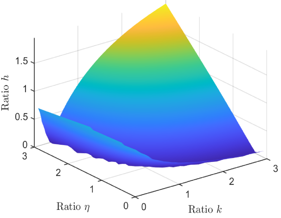
Figure 4: The relationship among three parameters $\eta$, $k$, and $h$ under the asymmetric condition determined in Eq. (28).

Due to the demanding requirements in practical experiments to prepare two cavities with identical dissipation rates, they are difficult to get. Considering the asymmetric case ($\gamma_{1}\neq\gamma_{2}$ i.e., $\eta\neq 1$) is meaningful for the study of EP3. By combining the pseudo-Hermitian condition in Eq. (19) with the EP3 condition in Eq. (23), we derive the following relationship among the three parameters $\eta$, $k$, and $h$, then we have

$$\frac{18}{\sqrt{3}}hk=\sqrt{\frac{\left[1+k^{2}\eta^{3}-h^{2}\left(1+\eta\right)^{3}\right]\left\{1+6\eta\left(1+2\eta\right)+h^{2}\left(\eta^{2}-1\right)^{3}-\eta^{3}\left[k^{2}\left(\eta+2\right)^{3}-8\right]\right\}^{2}}{\eta^{3}\left(1+\eta\right)^{3}\left(1+\eta+\eta^{2}\right)^{3}}}.$$ (28)

In Fig. 2, we show the variation of the ratio $h$ defined as $J/g_{1}$ with respect to the coupling strengths ratio $k$, which is ${g}_{2}/g_{1}$ under symmetrical conditions by using Eq. (27). It can be observed for $k<1$ and $J<g_{1}$. When $k=1$, we have $h=0$, indicating no coupling between the cavities $b_{1}$ and $b_{2}$. For $k>1$, $h$ increases with the enhancement of $k$. With Eq. (28), we plot a three-dimensional figure that describes the analytical expression of the relationship among parameters under asymmetric conditions ($\gamma_{1}\neq\gamma_{2}$) in Fig. 4. As $\eta$ and $k$ grow, $h$ decreases from $1$ to $0$ and then increases.

In Fig. 3, we provide a representation of the spectrum distributions corresponding to the effective Hamiltonian $\hat{H}_{\rm{Meff}}$ from Eq. (5) plotted as a function of the coupling strength $g_{1}$ under symmetric conditions with $\eta=1$. In particular, this analysis focuses on two different cases: $k=1$ (corresponding to the condition $g_{1}=g_{2}$) and $k=2$ ($g_{2}=2g_{1}$). If $g_{1}$ falls below $g_{\mathrm{min}}$ (as plotted by the green areas), no eigenvalues are present in the system due to the absence of pseudo-hermiticity.

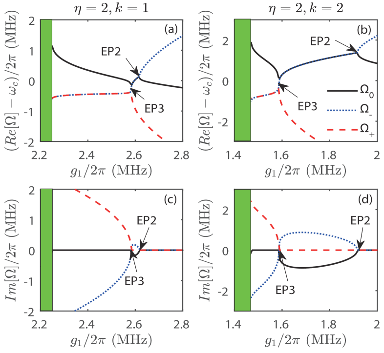
Figure 5: Under the asymmetric case $\gamma_{1}\neq\gamma_{2}$ ($\eta\neq 1$, where we choose $\eta=2$), the eigenvalues (both real and imaginary parts) of the effective Hamiltonian in Eq. (5) are plotted as a function of the coupling strength $g_{1}$ between the cavity $a$ and the cavity $b_{1}$. (a) and (c) respectively display the real and imaginary parts of the eigenvalues $\Omega_{\pm}$ and $\Omega_{0}$ corresponding to $g_{1}$ under the condition of $k=1$. (b) and (d) correspond to $g_{1}$ for the case with $k=2$. The remaining parameters are set to $\kappa_{1}/2\pi=\kappa_{2}/2\pi=4.5$ MHz and $\gamma_{2}/2\pi=1.5$ MHz. In contrast to Fig. 3 under symmetric conditions, EP2 and EP3 are distinguished in both cases plotted in Fig. 5

Figure 3(a) and (c) respectively display the real and imaginary parts of the eigenvalues $\Omega_{\pm}$ and $\Omega_{0}$ as they vary with $g_{1}$ for $k=1$. The critical coupling strength of $g_{\mathrm{EP3}}/2\pi=1.732$ MHz marks a different division in these figures. The eigenvalues exhibit different behaviors in two different ranges: $g_{\mathrm{min}}\leqslant g_{1}<g_{\mathrm{EP3}}$ and $g_{1}>g_{\mathrm{EP3}}$. For the first range ($g_{\mathrm{min}}\leqslant g_{1}<g_{\mathrm{EP3}}$), the eigenvalues $\Omega_{\pm}$ form a complex-conjugate pair (plotted by red dashed and blue dotted lines), while $\Omega_{0}$ remains real (black solid lines). At $g_{1}=g_{\mathrm{EP3}}$ (i.e., the EP3), the three eigenvalues $\Omega_{\pm}$ and $\Omega_{0}$ converge to $\Omega_{\mathrm{EP3}}=\omega_{c}$. For the second range ($g_{1}>g_{\mathrm{EP3}}$), all three eigenvalues are real.

Figure 3(b) and (d) respectively correspond to the variations of the real and imaginary parts of the eigenvalues with $g_{1}$ for $k=2$. Unlike the case with $k=1$, we observe the presence of two critical coupling strengths $g_{\mathrm{EP3}}/2\pi=1.095$ MHz and $g_{\mathrm{EP2}}/2\pi=1.245$ MHz. The eigenvalues possess a real eigenvalue and a pair of complex-conjugate pair within the ranges of $g_{\mathrm{min}}\leqslant g_{1}<g_{\mathrm{EP3}}$ and $g_{\mathrm{EP3}}<g_{1}<g_{\mathrm{EP2}}$, while they are all real eigenvalues at $g_{1}\geqslant g_{\mathrm{EP3}}$. In this situation, besides the occurrence of the EP3 at $g_{1}=g_{\mathrm{EP3}}$ where three eigenvalues coalesce, similar to the case of $k=1$, there is another EP2 at $g_{1}=g_{\mathrm{EP2}}$ where two eigenvalues merge, which is different from the previous case.

Figure 5 presents the variation of the real and imaginary parts of the eigenvalues $\Omega_{\pm}$ and $\Omega_{0}$ as a function of the coupling strength $g_{1}$ in an asymmetric case with $\eta=2$. Figure 5(a) and (c) show the situation of $k=1$, while Figs. 5(b) and (d) correspond to $k=2$. The remaining parameters are set as $\kappa_{1}=\kappa_{2}=3$ MHz and $\gamma_{1}=3$ MHz. In contrast to Fig. 3 with the symmetric case, both EP2 and EP3 can be observed in each panel of Fig. 5 at the same time. The detailed analysis of these figures is similar to Fig. 3(b) and (d) from the previous section, which will not be repeated here.

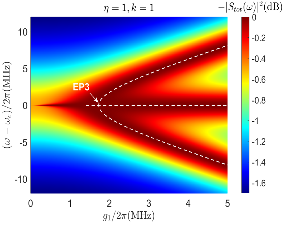
Figure 6: The output spectrum $|S_{tot}(\omega)|^{2}$ in Eq. (31) varies with the coupling strength $g_{1}$ and the frequency detuning $\omega-\omega_{c}$ between the input field and the cavity $a$ in the symmetric case of $\eta=1$. The minimum value of the output spectrum (the third-dimensional coordinate in the figure corresponds to the maximum value, i.e., the dark red contour) represents the CPA denoted as ${a}_{1}^{(out)}(\omega)={a}_{2}^{(out)}(\omega)=0$. The corresponding CPA frequency coincides with the real eigenvalue of the effective Hamiltonian in Eq. (5) in Fig. 3(a). The white dashed lines indicate the eigenvalues, where EP3 is marked in the figure. Other parameters are the same as Fig. 3.

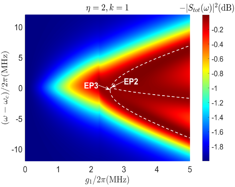
Figure 7: The output spectrum $|S_{tot}(\omega)|^{2}$ in the asymmetric case of $\gamma_{1}\neq\gamma_{2}$ ($\eta=2$) based on Eq. (31). Other parameters are the same as Fig. 5.

III.3 The output spectrum

In this section, we derive the total output spectrum of the cavity associated with the system and demonstrate that pseudo-hermiticity can be identified through analysis of this spectrum. In Sec. II.2, we discuss that the key requirement for CPA to occur is related to the two input fields ${a}_{1}^{(in)}(\omega)$ and ${a}_{2}^{(in)}(\omega)$ in Eq. (11). Using this equation, we can rewrite the expressions for the two outgoing fields, which are given by Eq. (10)

$${a}_{1}^{(out)}(\omega)=S_{1}(\omega){a}_{1}^{(in)}(\omega),$$ (29)

$${a}_{2}^{(out)}(\omega)=S_{2}(\omega){a}_{2}^{(in)}(\omega),$$

where $S_{1}(\omega)$ and $S_{2}(\omega)$ respectively representing the output coefficients at ports 1 and 2 corresponding to the frequency of the input fields:

$$S_{1}(\omega)=\frac{2\kappa_{1}+2\kappa_{2}}{(\kappa_{1}+\kappa_{2})+i(\omega_{c}-\omega)+\sigma(\omega)}-1,$$

$$S_{2}(\omega)=S_{1}(\omega).$$ (30)

In this case, we introduce a total output spectrum denoted as $|S_{tot}(\omega)|^{2}$, which serves to describe the input-output characteristics of the system

$$|S_{tot}(\omega)|^{2}=|S_{1}(\omega)|^{2}+|S_{2}(\omega)|^{2}.$$ (31)

The magnitude squared of the total output spectrum $|S_{tot}(\omega)|^{2}=0$ vanishes when the conditions specified in the second and third terms of Eq. (12) are met at $\omega=\omega_{\mathrm{CPA}}$.

The total output spectrum magnitude squared denoted as $|S_{tot}(\omega)|^{2}$ is plotted against the coupling strength $g_{1}$ and the frequency detuning $\omega-\omega_{c}$ of the two input fields relative to the cavity in Figs. 6 and 7 for $\eta=1$ and $\eta=2$, respectively. The minima observed in the total output spectrum (highlighted by the dark red contour) correspond to the condition of CPA, where both output fields ${a}_{1}^{(out)}$ and ${a}_{2}^{(out)}$ vanish. As expected, the frequencies at which CPA occurs coincide with the real eigenfrequencies of the effective pseudo-Hermitian Hamiltonian $\hat{H}_{\rm{Meff}}$ in Eq. (5). Here, the real eigenvalues are marked by white dashed lines. By measuring the total output spectrum of the microwave cavity, one can demonstrate the energy spectra and identify EP2 and EP3.

IV Non-Markovian model and effective Hamiltonian

Many physical phenomena particularly within the field of quantum optics are accurately captured by Markovian processes. However, these processes break down when the memory time of the environment is not negligible compared to the characteristic time of the system, where non-Markovian effects become predominant. Given that all practical quantum systems are inherently open due to inevitable strong environmental couplings GardinerBerlin2000 ; Li0621242010 ; Franco13450532013 ; Caruso12032014 , the significance of non-Markovian dynamics in such open systems should be taken into account. In this section, we assume that the environments of the two ports with the cavity $a$ are non-Markovian, where the environments are composed of a series of bosonic modes, while the other two environments coupling with cavities $b_{1}$ and $b_{2}$ are Markovian via dissipations $\gamma_{1}$ and $\gamma_{2}$, which is introduced phenomenologically (complete derivations with non-Markovian effects will be considered in Sec. VIII). The cavity is coupled to the $k$th mode (eigenfrequency $\omega_{k}$ and $\Omega_{k}$) of the non-Markovian environment via the annihilation (creation) operators $\hat{c}_{k}(\hat{c}^{{\dagger}}_{k})$ and $\hat{d}_{k}(\hat{d}^{{\dagger}}_{k})$.

Defining a rotating frame at the same frequency $\omega_{p}$ of the two input fields ($\hat{a}_{1}^{(in)}$ and $\hat{a}_{2}^{(in)}$) with $\hat{U}=\exp[-i\omega_{p}(\hat{a}^{\dagger}\hat{a}+\hat{b}_{1}^{\dagger}\hat{b}_{1}+\hat{b}_{2}^{\dagger}\hat{b}_{2}+\sum_{k}\hat{c}_{k}^{\dagger}\hat{c}_{k}+\sum_{k}\hat{d}_{k}^{\dagger}\hat{d}_{k})t]$, the total Hamiltonian can be written as

$$\hat{H}_{\rm{NM}} =\Delta_{c}\hat{a}^{\dagger}\hat{a}+\sum_{j=1,2}\left[\Delta_{j}\hat{b}_{j}^{\dagger}\hat{b}_{j}+g_{j}(\hat{a}^{\dagger}b_{j}+\hat{a}\hat{b}_{j}^{\dagger})\right]$$

$$+J(\hat{b}_{1}^{\dagger}\hat{b}_{2}+\hat{b}_{1}\hat{b}_{2}^{\dagger})+\sum_{k}\delta_{k}\hat{c}_{k}^{\dagger}\hat{c}_{k}+\sum_{k}\Delta_{k}\hat{d}_{k}^{\dagger}\hat{d}_{k}$$ (32)

$$+i\sum_{k}(g_{k}\hat{a}\hat{c}_{k}^{\dagger}-g_{k}^{*}\hat{a}^{\dagger}\hat{c}_{k})+i\sum_{k}(G_{k}\hat{a}\hat{d}_{k}^{\dagger}-G_{k}^{*}\hat{a}^{\dagger}\hat{d}_{k}),$$

where $g_{k}$ and $G_{k}$ denote the coupling strengths between the two ports of the cavity $a$ and the environments with frequency detunings $\delta_{k}=\omega_{k}-\omega_{p}$ and $\Delta_{k}=\Omega_{k}-\omega_{p}$. The Heisenberg equation with Eq. (32) can be given by

$$\frac{d}{dt}\hat{a}(t)= -i\Delta_{c}\hat{a}(t)-ig_{1}\hat{b_{1}}(t)-ig_{2}\hat{b}_{2}(t)$$

$$-\sum_{k}g_{k}^{*}\hat{c}_{k}(t)-\sum_{k}G_{k}^{*}\hat{d}_{k}(t),$$

$$\frac{d}{dt}\hat{b}_{1}(t)= -i(\Delta_{1}-i\gamma_{1})\hat{b}_{1}(t)-ig_{1}\hat{a}(t)-iJ\hat{b_{2}}(t),$$

$$\frac{d}{dt}\hat{b}_{2}(t)= -i(\Delta_{2}-i\gamma_{2})\hat{b}_{2}(t)-ig_{2}\hat{a}(t)-iJ\hat{b_{1}}(t),$$

$$\frac{d}{dt}\hat{c}_{k}(t)= -i\omega_{k}\hat{c}_{k}(t)+g_{k}\hat{a}(t),$$

$$\frac{d}{dt}\hat{d}_{k}(t)= -i\Omega_{k}\hat{d}_{k}(t)+G_{k}\hat{a}(t).$$ (33)

Solving Eq. (33) obtains the environmental operators for $t\geqslant 0$

$$\hat{c}_{k}(t) =\hat{c}_{k}(0)e^{-i\delta_{k}t}+g_{k}\int_{0}^{t}\hat{a}(\tau)e^{-i\omega_{k}(t-\tau)}d\tau,$$ (34)

$$\hat{d}_{k}(t) =\hat{d}_{k}(0)e^{-i\Delta_{k}t}+G_{k}\int_{0}^{t}\hat{a}(\tau)e^{-i\Omega_{k}(t-\tau)}d\tau,$$

which are divided into two components: the initial term represents the evolution of the non-Markovian environmental field, while the subsequent term reflects the feedback of non-Markovian effects from the environment to the cavity. Substituting Eq. (34) into Eq. (33), the integro-differential equation for the cavity operator yields

$$\frac{d}{dt}\hat{a}(t)= -i\Delta_{c}\hat{a}(t)-i\sum_{j=2}g_{j}\hat{b}_{j}(t)+\hat{K}_{1}(t)$$ (35)

$$+\hat{K}_{2}(t)-\int_{0}^{t}\hat{a}(\tau)[f_{1}(t-\tau)+f_{2}(t-\tau)]d\tau,$$

where

$$\hat{K}_{1}(t)= -\sum_{k}g_{k}^{*}\hat{c}_{k}(0)e^{-i\omega_{k}t}=\int_{-\infty}^{\infty}\kappa^{*}_{1}(t-\tau)\hat{a}^{(in)}_{1}(\tau)d\tau,$$

$$\hat{K}_{2}(t)= -\sum_{k}G_{k}^{*}\hat{d}_{k}(0)e^{-i\Omega_{k}t}=\int_{-\infty}^{\infty}\kappa^{*}_{2}(t-\tau)\hat{a}^{(in)}_{2}(\tau)d\tau$$

denote the couplings between the cavity and the input field of the non-Markovian environment with the defined input field operators $\hat{a}^{(in)}_{1}(t)=-\frac{1}{\sqrt{2\pi}}\sum_{k}\hat{c}_{k}(0)e^{-i\omega_{k}t}$ and $\hat{a}^{(in)}_{2}(t)=-\frac{1}{\sqrt{2\pi}}\sum_{k}\hat{d}_{k}(0)e^{-i\Omega_{k}t}$. In the continuum limit, the impulse response functions are transformed into

$${\kappa_{1}}(t-\tau)= \frac{1}{{\sqrt{2\pi}}}\int_{-\infty}^{+\infty}{{e^{i\omega(t-\tau)}}}g(\omega)d\omega,$$ (36)

$${\kappa_{2}}(t-\tau)= \frac{1}{{\sqrt{2\pi}}}\int_{-\infty}^{+\infty}{{e^{i\omega(t-\tau)}}}G(\omega)d\omega,$$

by the replacements with $g_{k}\to g(\omega)$ and $G_{k}\to G(\omega)$. The correlation function occupies a significant role and serves as a memory function in the interactions between the cavity and their environments

$${f_{1}}(t)=\int_{-\infty}^{+\infty}{{J_{1}}(\omega){e^{-i\omega t}}d\omega=\int_{-\infty}^{+\infty}{{\kappa_{1}}}(-\xi)\kappa_{1}^{*}(t-\xi)d\xi,}$$ (37)

$${f_{2}}(t)=\int_{-\infty}^{+\infty}{{J_{2}}(\omega){e^{-i\omega t}}d\omega=\int_{-\infty}^{+\infty}{{\kappa_{2}}}(-\xi)\kappa_{2}^{*}(t-\xi)d\xi,}$$

where $J_{1}(\omega)=|g{(\omega)}|^{2}$ and $J_{2}(\omega)=|G{(\omega)}|^{2}$ are the spectral density of the environments. Similarly, the solutions for the environmental operators can be obtained by

$$\hat{c}_{k}(t) =\hat{c}_{k}(t_{1})e^{-i\omega_{k}(t-t_{1})}-g_{k}\int_{t}^{t_{1}}\hat{a}(\tau)e^{-i\omega_{k}(t-\tau)}d\tau,$$ (38)

$$\hat{d}_{k}(t) =\hat{d}_{k}(t_{1})e^{-i\Omega_{k}(t-t_{1})}-G_{k}\int_{t}^{t_{1}}\hat{a}(\tau)e^{-i\Omega_{k}(t-\tau)}d\tau,$$

with $t\leqslant t_{1}$, which leads to another integro-differential equation

$$\frac{d}{dt}\hat{a}(t)= -i\Delta_{c}\hat{a}(t)-i\sum_{j=2}g_{j}\hat{b}_{j}(t)-\hat{K}_{1}^{{}^{\prime}}(t)-\hat{K}_{2}^{{}^{\prime}}(t)$$ (39)

$$+\int_{t}^{t_{1}}\hat{a}(\tau)[f_{1}(t-\tau)+f_{2}(t-\tau)]d\tau,$$

where we respectively have defined the externally driven environments and the output-field operators as

$$\hat{K}^{{}^{\prime}}_{1}(t)= \sum_{k}g_{k}^{*}\hat{c}_{k}(t_{1})e^{-i\omega_{k}(t-t_{1})}$$

$$= \int_{-\infty}^{\infty}\kappa^{*}_{1}(t-\tau)\hat{a}^{(out)}_{1}(\tau)d\tau,$$

$$\hat{K}^{{}^{\prime}}_{2}(t)= \sum_{k}G_{k}^{*}\hat{d}_{k}(t_{1})e^{-i\Omega_{k}(t-t_{1})}$$

$$= \int_{-\infty}^{\infty}\kappa^{*}_{2}(t-\tau)\hat{a}^{(out)}_{2}(\tau)d\tau.$$ (40)

where

$$\hat{a}^{(out)}_{1}(t) =\frac{1}{\sqrt{2\pi}}\sum_{k}\hat{c}_{k}(t_{1})e^{-i\omega_{k}(t-t_{1})}$$

$$\hat{a}^{(out)}_{2}(t) =\frac{1}{\sqrt{2\pi}}\sum_{k}\hat{d}_{k}(t_{1})e^{-i\Omega_{k}(t-t_{1})}.$$ (41)

By setting Eq. (35) being equal to Eq. (39) with the substitution $t_{1}\rightarrow t$ Diosi0341012012 , we derive the non-Markovian input-output relation for the $\nu$th port of the cavity $a$

$$\hat{a}_{\nu}^{(out)}(t)+\hat{a}_{\nu}^{(in)}(t)=\int_{0}^{t}\kappa_{\nu}(\tau-t)\hat{a}(\tau)d\tau,$$ (42)

where $\kappa_{\nu}(t-\tau)$ is given by Eq. (36). Taking the impulse response functions $\kappa_{\nu}(t)=\lambda_{\nu}\sqrt{\Gamma_{\nu}}e^{\lambda_{\nu}t}\theta(-t)$, we can obtain the correlation functions $f_{\nu}(t)=\frac{1}{2}\lambda_{\nu}\Gamma_{\nu}e^{-\lambda_{\nu}|t|}$ by Eq. (37), which leads to the spectral response functions $g(\omega)=\frac{1}{\sqrt{2\pi}}\int_{-\infty}^{+\infty}e^{-i\omega t}\kappa_{1}(t)dt$ and $G(\omega)=\frac{1}{\sqrt{2\pi}}\int_{-\infty}^{+\infty}e^{-i\omega t}\kappa_{2}(t)dt$ with the Fourier transform to Eq. (36) as Jack0438032001 ; Groblacher76062015

$$g(\omega)=\sqrt{\frac{\Gamma_{1}}{2\pi}}\frac{\lambda_{1}}{\lambda_{1}-i\omega},\ G(\omega)=\sqrt{\frac{\Gamma_{2}}{2\pi}}\frac{\lambda_{2}}{\lambda_{2}-i\omega},$$ (43)

where $\lambda_{\nu}$ represents the non-Markovian environmental spectral width, while $\Gamma_{\nu}$ denotes the cavity dissipation at the input and output ports. Consequently, the Lorentzian spectral densities Xiong0321072012 ; Shen0121562017 ; Jing2404032010 are

$$J_{\nu}(\omega)=\frac{\Gamma_{\nu}}{2\pi}\frac{\lambda_{\nu}^{2}}{\lambda_{\nu}^{2}+\omega^{2}},$$ (44)

which represent a Gaussian Ornstein-Uhlenbeck process Jing2404032010 ; Uhlenbeck8231930 ; Gillespie20841996 . The impulse response functions $\kappa_{\nu}(t)$ and correlation function $f_{\nu}(t)$ can also be realized through the pseudomode theory (see Appendix A). $\theta(t-\tau)$ denotes the unit step function defined as $\theta(t-\tau)=1$ for $t-\tau\geqslant 0$ and $\theta(t-\tau)=0$ otherwise. In particular, the memory effect inherent to the non-Markovian environment disappears as the spectral width $\lambda_{\nu}$ tends to infinity. In this case, the environmental spectral density $J_{\nu}(\omega)$ approximates to ${\Gamma_{\nu}}/{2\pi}$, which corresponds to $g(\omega)=\sqrt{{\Gamma_{1}}/{2\pi}}$ and $G(\omega)=\sqrt{\Gamma_{2}}/{2\pi}$ characterizing the case under the Markovian approximation. Based on Eqs. (36) and (37), we derive $\kappa_{\nu}(t)\to\sqrt{\Gamma_{\nu}}\delta(t)$ and $f_{\nu}(t)\to\Gamma_{\nu}\delta(t)$. Substituting these results into Eq. (42) yields the input-output relation under the Markovian approximation

$$\hat{a}_{\nu}^{(out)}(t)+\hat{a}_{\nu}^{(in)}(t)=\sqrt{\Gamma_{\nu}}\hat{a}(t),$$ (45)

which is equivalent to that defined in Refs. GardinerBerlin2000 ; Walls1994 ; Scully1997 .

IV.1 Effective Hamiltonian in non-Markovian regimes with $\lambda_{1}=\lambda_{2}$ and $\Gamma_{1}=\Gamma_{2}$

For the first case, we consider the spectral widths $\lambda_{1}=\lambda_{2}$ and dissipations $\Gamma_{1}=\Gamma_{2}$, which leads to $\hat{K}_{1}(t)=\hat{K}_{2}(t)\equiv\hat{K}(t)$. Combined with Eq. (39), the Heisenberg equation in Eq. (33) becomes

$$\frac{d}{dt}\hat{a}(t)= -i\Delta_{c}\hat{a}(t)-ig_{1}\hat{b_{1}}(t)-ig_{2}\hat{b}_{2}(t)$$ (46)

$$+2\hat{K}(t)-2\int_{0}^{t}\hat{a}(\tau)f(t-\tau)d\tau,$$

$$\frac{d}{dt}\hat{b}_{1}(t)= -i(\Delta_{1}-i\gamma_{1})\hat{b}_{1}(t)-ig_{1}\hat{a}(t)-iJ\hat{b_{2}}(t),$$

$$\frac{d}{dt}\hat{b}_{2}(t)= -i(\Delta_{2}-i\gamma_{2})\hat{b}_{2}(t)-ig_{2}\hat{a}(t)-iJ\hat{b_{1}}(t).$$

With CPA, the effective non-Markovian Hamiltonian $\hat{H}_{\rm{NMeff}}$ of the system can be expressed as (see Appendix B for more details)

$$\hat{H}_{\rm{NMeff}}=\begin{pmatrix}\Delta_{c}&g_{1}&g_{2}&-2ig\\ g_{1}&\Delta_{1}-i\gamma_{1}&J&0\\ g_{2}&J&\Delta_{2}-i\gamma_{2}&0\\ ig&0&0&i\lambda\end{pmatrix},$$ (47)

where we have defined $g=\sqrt{{\lambda\Gamma}/{2}}$.

IV.2 CPA conditions in non-Markovian regimes

Making the modified Laplace transformation to Eq. (46), we find the cavity equations

$$-i\omega a(\omega)= -i\Delta_{c}a(\omega)-ig_{1}b_{1}(\omega)-ig_{2}b_{2}(\omega)$$ (48)

$$+\tilde{\kappa}_{1}(\omega)[a_{in}^{(1)}(\omega)-a_{in}^{(1)}(i\lambda_{1})]-a(\omega)f_{1}(\omega)$$

$$+\tilde{\kappa}_{2}(\omega)[a_{in}^{(2)}(\omega)-a_{in}^{(2)}(i\lambda_{2})]-a(\omega)f_{2}(\omega),$$

$$-i\omega b_{1}(\omega)= -i(\Delta_{1}-i\gamma_{1})b_{1}(\omega)-ig_{1}a(\omega)-iJb_{2}(\omega),$$

$$-i\omega b_{2}(\omega)= -i(\Delta_{2}-i\gamma_{2})b_{2}(\omega)-ig_{2}a(\omega)-iJb_{1}(\omega),$$

where

$$\tilde{\kappa}_{\nu}(\omega)= \int_{-\infty}^{0}\kappa_{\nu}^{*}(t^{\prime})e^{i\omega t^{\prime}}dt^{\prime},$$

$$a_{in}^{(\nu)}(\omega)= \int_{0}^{\infty}a_{in}^{(\nu)}(t^{\prime})e^{i\omega t^{\prime}}dt^{\prime},$$ (49)

$$f_{\nu}(\omega)= \int_{0}^{\infty}f_{\nu}^{*}(t^{\prime})e^{i\omega t^{\prime}}dt^{\prime}.$$

Eq. (48) can be rewritten as (more details can be found in Appendix C)

$$-i\omega a(\omega)= -i\Delta_{c}a(\omega)-ig_{1}b_{1}(\omega)-ig_{2}b_{2}(\omega)-a(\omega)f_{1}(\omega)$$ (50)

$$-a(\omega)f_{2}(\omega)+\tilde{\kappa}_{1}(\omega)a_{in}^{(1)}(\omega)+\tilde{\kappa}_{2}(\omega)a_{in}^{(2)}(\omega),$$

$$-i\omega b_{1}(\omega)= -i(\Delta_{1}-i\gamma_{1})b_{1}(\omega)-ig_{1}a(\omega)-iJb_{2}(\omega),$$

$$-i\omega b_{2}(\omega)= -i(\Delta_{2}-i\gamma_{2})b_{2}(\omega)-ig_{2}a(\omega)-iJb_{1}(\omega),$$

which gives

$$a{(\omega)}=\frac{\tilde{\kappa}_{1}(\omega)a_{in}^{(1)}(\omega)+\tilde{\kappa}_{2}(\omega)a_{in}^{(2)}(\omega)}{f_{1}(\omega)+f_{2}(\omega)+i(\Delta_{c}-\omega)+\sigma(\omega)},$$ (51)

where $\sigma(\omega)$ is given by Eq. (9). By incorporating Eq. (42), the input-output relationship of non-Markovian systems in the frequency domain reads

$$\begin{gathered}a_{i}^{(in)}(\omega)+a_{i}^{(out)}(\omega)=a(\omega)\kappa_{i}(-\omega).\end{gathered}$$ (52)

When coherent perfect absorption occurs $a_{i}^{(out)}(\omega)=0$, we have $a_{1}^{(in)}(\omega)/a_{2}^{(in)}(\omega)=\kappa_{1}(-\omega)/\kappa_{2}(-\omega).$ With Eq. (51), we obtain

$$a_{i}^{(out)}(\omega)= \frac{\kappa_{i}(-\omega)(\tilde{\kappa}_{1}(\omega)a_{in}^{(1)}(\omega)+\tilde{\kappa}_{2}(\omega)a_{in}^{(2)}(\omega))}{f_{1}(\omega)+f_{2}(\omega)+i(\Delta_{c}-\omega)+\sum(\omega)}$$ (53)

$$-a_{i}^{(in)}(\omega),$$

where the self-energy between the two cavities under the frequency domain is

$$\sigma(\omega)= \kappa_{1}(-\omega)\tilde{\kappa}_{1}(\omega)+\kappa_{2}(-\omega)\tilde{\kappa}_{2}(\omega)$$ (54)

$$-f_{1}(\omega)-f_{2}(\omega)-i(\Delta_{c}-\omega).$$

IV.3 Pseduo-Hermitian Hamiltonian in non-Markovian regimes

In the subsequent section, we study the parametric requisites that ensure the pseudo-Hermiticity of the effective Hamiltonian $\hat{H}_{\rm{NMeff}}$ in Eq. (47). This particular Hamiltonian under consideration possesses a quartet of eigenvalues. According to the method in Ref. Mostafazadeh2052002 , $\hat{H}_{\rm{NMeff}}$ acquires pseudo-Hermitian properties if all four of its eigenvalues are real. To satisfy this condition, we solve the equation $\mathrm{Det}(\hat{H}_{\rm{NMeff}}-\Omega I)=0$ as

$$\begin{vmatrix}\Delta_{c}-\Omega&g_{1}&g_{2}&-2ig\\ g_{1}&(\Delta_{1}-i\gamma_{1})-\Omega&J&0\\ g_{2}&J&(\Delta_{2}-i\gamma_{2})-\Omega&0\\ ig&0&0&i\lambda-\Omega\end{vmatrix}=0.$$ (55)

Based on the energy-spectrum characteristics described in the pseudo-Hermitian Hamiltonian framework Mostafazadeh2052002 , we have $\mathrm{Det}(\hat{H}_{\rm{NMeff}}^{*}-\Omega I)=0$ and

$$\begin{vmatrix}\Delta_{c}-\Omega&g_{1}&g_{2}&2ig\\ g_{1}&(\Delta_{1}+i\gamma_{1})-\Omega&J&0\\ g_{2}&J&(\Delta_{2}+i\gamma_{2})-\Omega&0\\ -ig&0&0&-i\lambda\end{vmatrix}=0,$$ (56)

serve as valid expressions. With Eqs. (55) and (56), the system’s parameters follow a set of constraints

$$\lambda-\gamma_{1}-\gamma_{2}=0,$$

$$\gamma_{1}\Delta_{1}+\gamma_{2}\Delta_{2}=0,$$ (57)

$${g_{1}}^{2}\gamma_{2}+{g_{2}}^{2}\gamma_{1}-\lambda(\Delta_{1}\Delta_{2}+\lambda\Gamma-\gamma_{1}\gamma_{2}-J^{2})=0,$$

$$g_{2}^{2}\Delta_{1}+g_{1}^{2}\Delta_{2}+\xi\Delta_{c}-2Jg_{1}g_{2}-\Gamma(\gamma_{2}\Delta_{1}+\gamma_{1}\Delta_{2})=0,$$

where the coefficient $\xi=J^{2}+\gamma_{1}\gamma_{2}-\Delta_{1}\Delta_{2}$.

V Fourth-order exceptional points in Non-Markovian regimes with same spectral widths

In this section, we investigate the EP4 under both symmetric and asymmetric conditions by solving the characteristic equation when the system parameters satisfy the pseudo-Hermitian condition with the same spectral width ($\lambda_{1}=\lambda_{2}$) of the non-Markovian environments and demonstrate that this EP4 can be observed through the measurement of the total output spectrum of the cavity. In this case, Eq. (55) becomes

$$a(\Omega-\Delta_{c})^{4}+b(\Omega-\Delta_{c})^{3}+$$ (58)

$$c(\Omega-\Delta_{c})^{2}+d(\Omega-\Delta_{c})+e=0,$$

where the parameters $a=1$, $b=-\Delta_{1}-\Delta_{2}+3\Delta_{c}$, $c=-g_{1}^{2}-g_{2}^{2}-J^{2}-\Gamma\lambda+\lambda^{2}-\gamma_{1}\gamma_{2}+\Delta_{1}\Delta_{2}+3\Delta_{c}^{2}-2(\Delta_{1}+\Delta_{2})\Delta_{c}$, $d=2g_{2}^{2}(\Delta_{1}-\Delta_{c})+2g_{1}^{2}(\Delta_{2}-\Delta_{c})-4Jg_{1}g_{2}-\lambda(\gamma_{2}\Delta_{1}+\gamma_{1}\Delta_{2})+\lambda(-2\Gamma+\lambda)\Delta_{c}-(\Delta_{1}+\Delta_{2})\Delta_{c}^{2}+\Delta_{c}^{3}$, and $e=2\Gamma(\gamma_{2}\Delta_{1}+\gamma_{1}\Delta_{2})\Delta_{c}-(J^{2}+\Gamma\lambda+\gamma_{1}\gamma_{2}-\Delta_{1}\Delta_{2})\Delta_{c}^{2}-g_{2}^{2}(\lambda\gamma_{1}+\Gamma\lambda_{2}+\Delta_{c}^{2})-g_{1}^{2}(\lambda\gamma_{2}+\Gamma\lambda_{1}+\Delta_{c}^{2})+\Gamma^{2}\lambda^{2}$.

According to the discriminant of the roots of a quartic equation, when the parameters satisfy $\Delta\equiv B^{2}-4AC=0$, there exist four equal real roots, where $A=D^{2}-3F$, $B=DF-9E^{2}$, and $C=F^{2}-3DE^{2}$ with

$$D=3b^{2}-8ac,$$ (59)

$$E=-b^{3}+4abc-8a^{2}d,$$

$$F=3b^{4}+16a^{2}c^{2}-16ab^{2}c+16a^{2}bd-64a^{3}e.$$

When $D=E=F=0$, Eq. (58) has a quadruple real root where $\Omega_{1}=\Omega_{2}=\Omega_{3}=\Omega_{4}=-\frac{b}{4a}=-\frac{2c}{3b}=-\frac{3d}{2c}=-\frac{4c}{d}$.

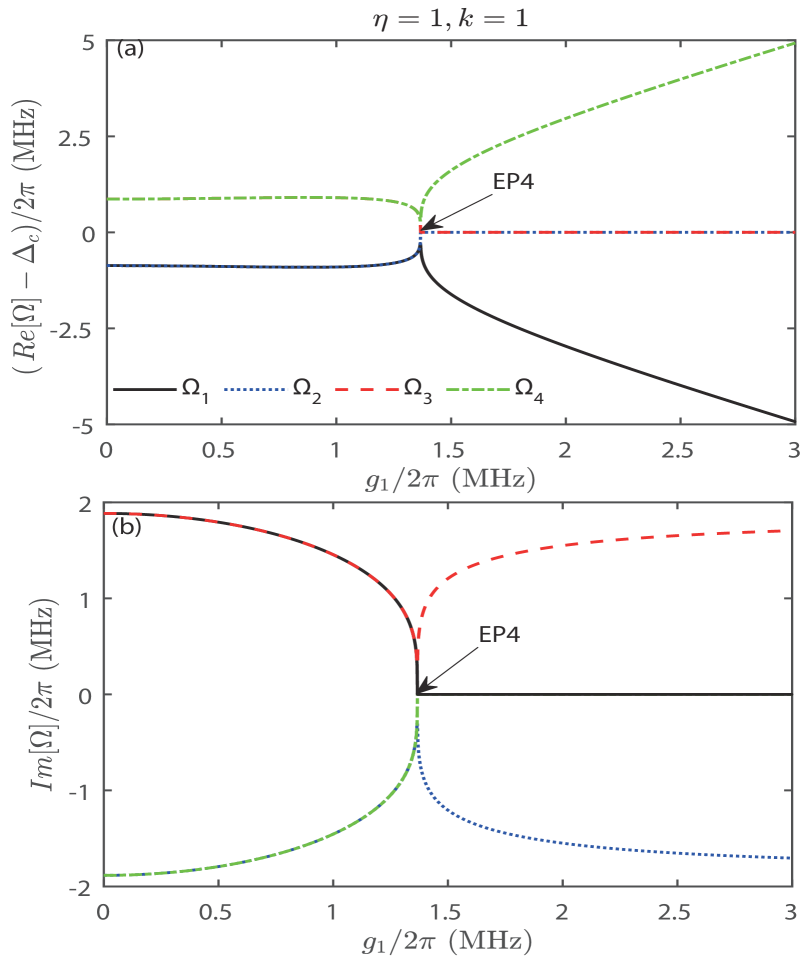
Figure 8: The dependence of the eigenvalues for the effective Hamiltonian $\hat{H}_{\rm{NMeff}}$ in Eq. (32) under pseudo-Hermitian conditions with non-Markovian effects (characterized by a small environmental spectral width $\lambda_{1}/2\pi=\lambda_{2}/2\pi=3.77$ MHz) versus the coupling strength $g_{1}$ in the symmetric case of $\eta=1$. Other parameters are set to $k=1$, $\gamma_{2}/2\pi=1.885$ MHz, and $g_{1}/2\pi=1.367$ MHz.

V.1 The symmetric case of $\gamma_{1}=\gamma_{2}$ and $\lambda_{1}=\lambda_{2}$

When the two cavities ($b_{1}$ and $b_{2}$) possess the same dissipation rates $\gamma_{1}=\gamma_{2}$ (i.e., $\eta=1$), combining with Eq. (18), the pseudo-Hermitian condition in Eq. (57) of the system then becomes

$$\lambda= 2\gamma_{2},$$ (60)

$$\Delta_{2}= -\Delta_{1},$$

$$\Gamma= \frac{(2h^{2}+k^{2}+1)g_{1}^{2}+2\gamma_{2}^{2}+2\Delta_{1}^{2}}{4\gamma_{2}},$$

$$\Delta_{c}= \frac{2hkg_{1}^{3}+(1-k^{2})g_{1}^{2}\Delta_{1}}{h^{2}g_{1}^{2}+\gamma_{2}^{2}+\Delta_{1}^{2}}.$$

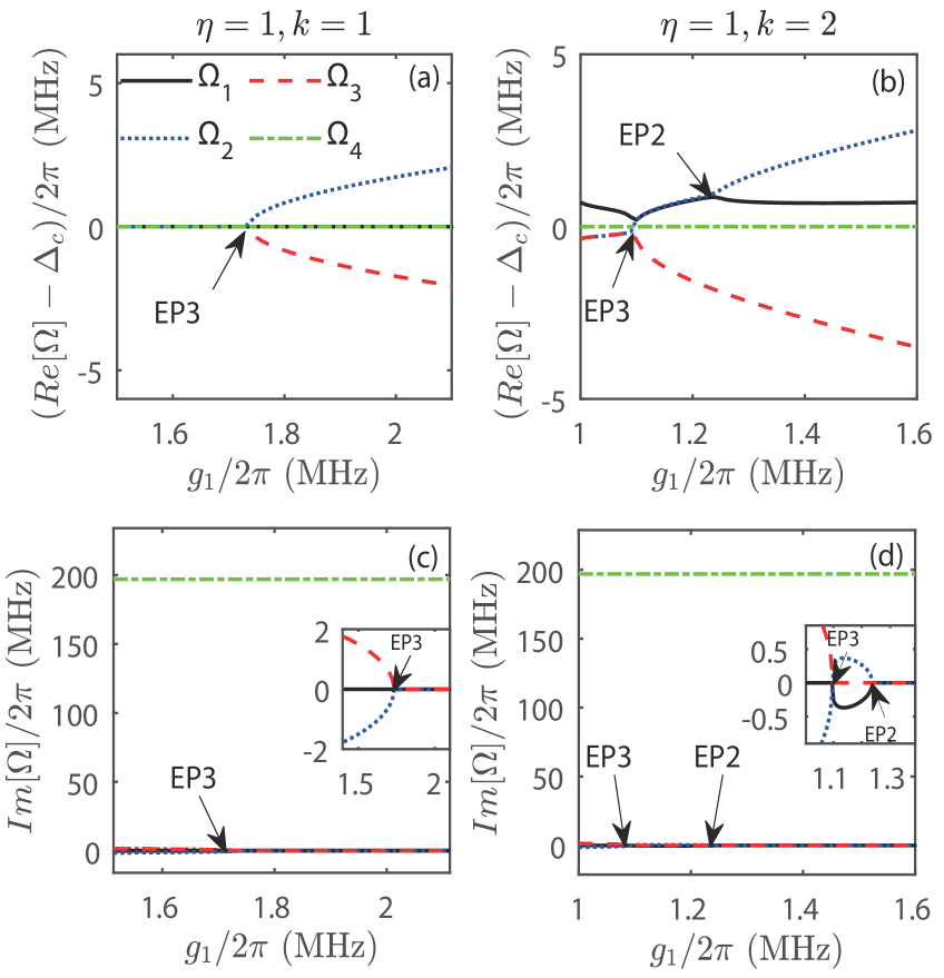
Figure 9: The variation of eigenvalues for the effective non-Markovian Hamiltonian $\hat{H}_{\rm{NMeff}}$ in Eq. (32) with coupling strength $g_{1}$ in the conversion to the Markovian case (with a larger environmental spectral width $\lambda$, specifically $\lambda_{1}/2\pi=\lambda_{2}/2\pi=200$ MHz) is investigated in the symmetric case of $\eta=1$. (a) and (c) respectively plot the real and imaginary parts for the case of $k=1$. (b) and (d) correspond to the real and imaginary parts for the case of $k=2$. Under the same parametric conditions, the results returning to Fig. 3 can be obtained.

Figure 8(a) and (b) respectively show the variations of the real and imaginary parts of the eigenvalues with respect to $g_{1}$ in the non-Markovian symmetric case (when dissipations are equal, i.e., $\gamma_{1}=\gamma_{2}$), where the critical coupling strength at EP4 is $g_{\mathrm{EP4}}=1.367$ MHz. For $g_{1}<g_{\mathrm{EP4}}$, the four eigenvalues form two pairs of complex conjugates. At EP4 and $g_{1}=g_{\mathrm{EP4}}$, all four eigenvalues coalesce and become real. As $g_{1}>g_{\mathrm{EP4}}$, the eigenvalues demonstrate two reals and a pair of complex conjugates. The remaining parameters are set as $g_{2}=g_{1}$ (i.e., $k=1$) and $\Gamma_{1}=\Gamma_{2}=1.637$ MHz.

In Fig. 9(a) and (c), we observe the evolution versus the coupling strength $g_{1}$ of the real and imaginary parts of the eigenvalues during the non-Markovian to Markovian conversion under symmetric conditions with $k=1$. Compared to the corresponding Fig. 3(a) and (c), the real parts in Fig. 9(a) and (b) show a remarkable characteristic: a high degree of consistency. However, the imaginary parts in Fig. 9(c) and (d) display an extra green dashed-dotted line, which indicates the different spectral width of the non-Markovian environments.

Moreover, Fig. 9(b) and (d) reveal novel characteristics in the variation of the real and imaginary parts of the eigenvalues during the non-Markovian to Markovian regimes under the same symmetric conditions but with an increased $k$ value of 2. In contrast to Fig. 3(b) and (d), an additional green dashed-dotted line appears in both the real and imaginary parts. In the real part, this line represents the zero eigenvalue, while in the imaginary part, it represents the spectral width of the non-Markovian environments.

With other parameters fixed (e.g., $\Gamma_{1}=\Gamma_{2}=2\gamma_{2}$), the above analysis not only deepens our understanding of the dynamical behavior of non-Markovian pseudo-Hermitian systems but also explicitly demonstrates how such systems can convert to Markovian regimes under specific symmetric conditions.

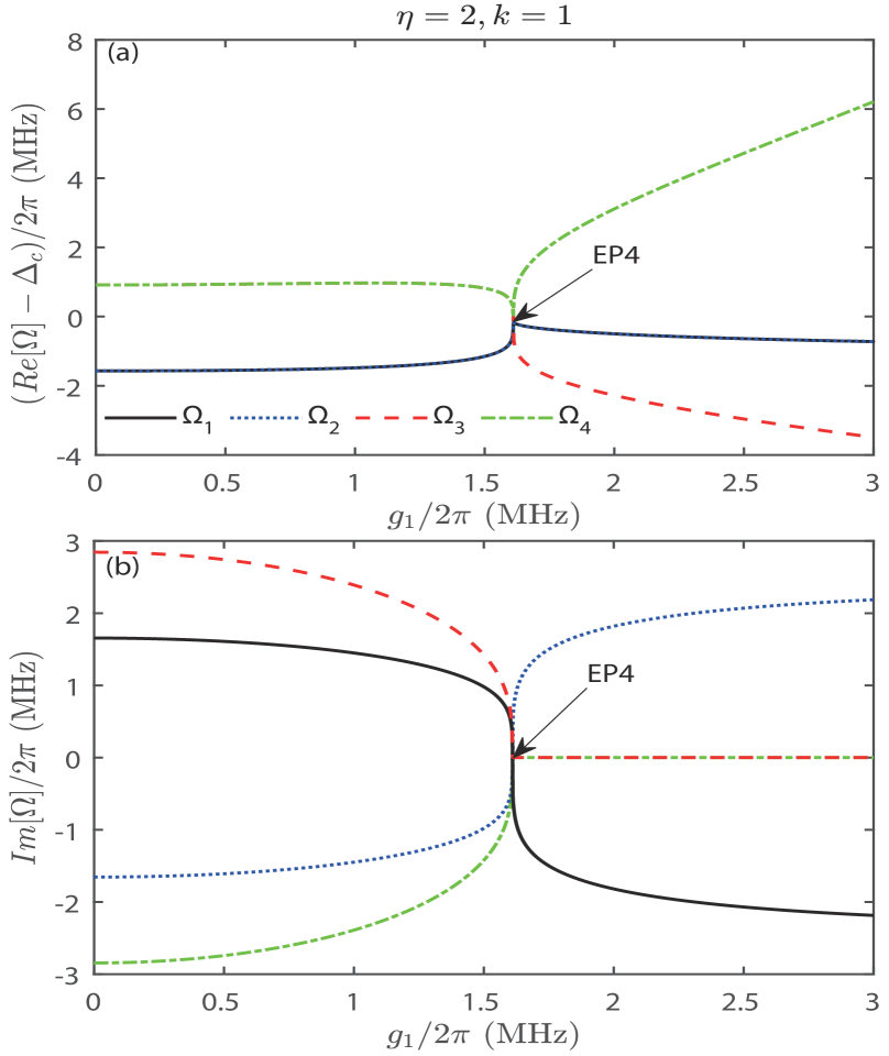
Figure 10: In the asymmetric case of $\gamma_{1}\neq\gamma_{2}$ ($\eta\neq 1$, taking $\eta=2$), the real and imaginary parts of eigenvalues for the effective Hamiltonian $\hat{H}_{\rm{NMeff}}$ in Eq. (32) vary with the coupling strength $g_{1}$ under pseudo-Hermitian conditions. Other parameters are set to $k=1$, $\lambda_{1}/2\pi=\lambda_{2}/2\pi=4.5$ MHz, $\gamma_{2}/2\pi=1.5$ MHz, and $g_{1}/2\pi=1.610$ MHz.

V.2 The asymmetric case of $\gamma_{1}\neq\gamma_{2}$ and $\lambda_{1}=\lambda_{2}$

When the dissipation rates of the two cavities ($b_{1}$ and $b_{2}$) are different ($\gamma_{1}\neq\gamma_{2}$), it is considered as an example with $\eta=2$ ($\gamma_{1}=2\gamma_{2}$). In this case, the pseudo-Hermitian condition in Eq. (57) of the system is given by

$$\lambda= \ 3\gamma_{2},\ \Delta_{2}=-2\Delta_{1},$$

$$\Gamma= \ \frac{3J^{2}+g_{1}^{2}+g_{2}^{2}+6\gamma_{2}^{2}+6\Delta_{1}^{2}}{9\gamma_{2}},$$ (61)

$$\Delta_{c}= \ \frac{6Jg_{1}g_{2}-3J^{2}\Delta_{1}+4g_{1}^{2}\Delta_{1}-4g_{2}^{2}\Delta_{1}-6\gamma_{2}^{2}\Delta_{1}-6\Delta_{1}^{3}}{3(J^{2}+2\gamma_{2}^{2}+2\Delta_{1}^{2})}.$$

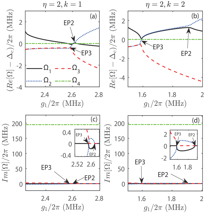
Figure 11: The evolution of the eigenvalues for the effective non-Markovian Hamiltonian $\hat{H}_{\rm{NMeff}}$ in Eq. (32) with varying coupling strength $g_{1}$ during the conversion towards the Markovian regime characterized by an increased environmental spectral width ($\lambda_{1}/2\pi=\lambda_{2}/2\pi=200$ MHz), is studied under asymmetric conditions, where $\gamma_{1}$ differs from $\gamma_{2}$ (i.e., $\eta=2$). For the case with $k=1$, (a) and (c) present the real and imaginary parts of these eigenvalues. Similarly, (b) and (d) respectively show the real and imaginary parts with $k=2$. Under identical parameter settings, the results in Fig. 5 are observed.

Figure 10(a) and (b) respectively display the variations of the real and imaginary parts of the eigenvalues with respect to $g_{1}$ in the non-Markovian asymmetric case (when dissipations are not equal, i.e., $\gamma_{1}=2\gamma_{2}$), where the critical coupling strength at the EP4 is $g_{\mathrm{EP4}}/2\pi=1.610$ MHz. The analysis is consistent with Fig. 8(a) and (b). Other parameters are set as $g_{2}=g_{1}$ (i.e., $k=1$) and $\Gamma_{1}/2\pi=\Gamma_{2}/2\pi=1.942$ MHz.

Figure 11(a) and (c) focus on the asymmetric condition with $k=1$, describing how the real and imaginary parts of the eigenvalues evolve with $g_{1}$ during the conversion from non-Markovian to Markovian regimes. In comparison to the corresponding sections in Fig. 5, a green dashed-dotted line in the real part plot marks the special state where the eigenvalue is zero, while a similar green dashed-dotted line appears in the imaginary part, representing the spectral width characteristics of the non-Markovian environment.

Figure 11(b) and (d) show the changes in the real and imaginary parts of the eigenvalues during the non-Markovian to Markovian regimes under the asymmetric case with $k=2$. The comparison with Fig. 5 once again highlights the addition of green dashed-dotted lines in both the real and imaginary parts, serving to identify the zero eigenvalue and the spectral width feature of the non-Markovian environments, respectively. We have also obtained the conversion from a non-Markovian pseudo-Hermitian system to a Markovian one under asymmetric conditions. Other parameters in this analysis are set to $\Gamma_{1}/2\pi=\Gamma_{2}/2\pi=4.5$ MHz.

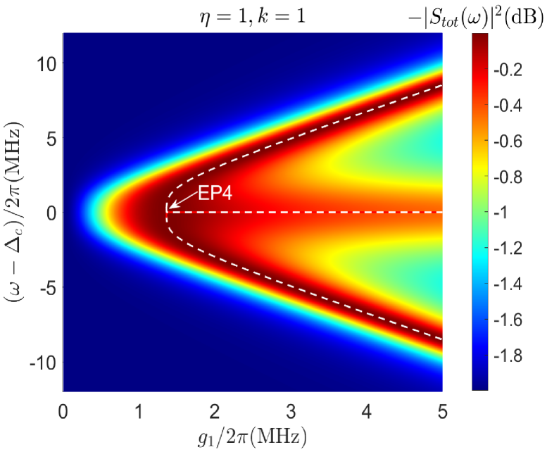
Figure 12: The output spectrum $|S_{\rm{NMtot}}(\omega)|^{2}$ in Eq. (63) varies with the coupling strength $g_{1}$ and the frequency detuning $\omega-\Delta_{c}$ between the input field and the cavity $a$ in the symmetric case of $\eta=1$ in non-Markovian regimes. Other parameters are the same as in Fig. 8.

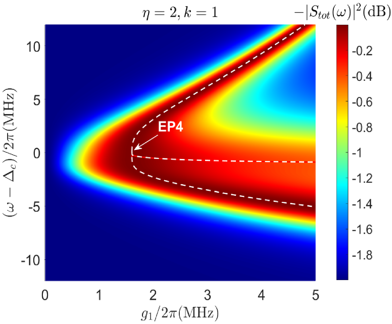
Figure 13: The output spectrum $|S_{\rm{NMtot}}(\omega)|^{2}$ in Eq. (63) varies with the coupling strength $g_{1}$ and the frequency detuning $\omega-\Delta_{c}$ between the input field and the cavity $a$ in the asymmetric case of $\eta=2$ in non-Markovian regimes. Other parameters are the same as in Fig. 10.

V.3 The output spectrum

In this section, we derive the total output spectrum of the cavity for the non-Markovian system and show that the pseudo-Hermiticity can be observed through the output spectrum

$$S(\omega)=\frac{\kappa_{1}(-\omega)\tilde{\kappa}_{1}(\omega)+\kappa_{2}(-\omega)\tilde{\kappa}_{2}(\omega)}{f_{1}(\omega)+f_{2}(\omega)+i(\Delta_{c}-\omega)+\sigma(\omega)}-1,$$ (62)

where we have defined a total output spectrum $|S_{\rm{NMtot}}(\omega)|^{2}$ to characterize the input-output property of the non-Markovian system

$$|S_{\rm{NMtot}}(\omega)|^{2}=2|S(\omega)|^{2}.$$ (63)

In Fig. 12, we choose the case with parameters $\eta=1$ and $k=1$ (this setting is also referenced in Fig. 8) to demonstrate how the output spectrum $S_{\rm{NMtot}}(\omega)$ dynamically varies with the coupling strength $g_{1}$ and the frequency detuning $\omega-\Delta_{c}$ between the input field and the cavity $a$. The case corresponding to Fig. 13 is that with $\eta=2$ and $k=1$ (which is also referenced in Fig. 10). By adopting the negative magnitude of $|S_{\rm{NMtot}}(\omega)|^{2}$ as the third dimension coordinate. With the peaks highlighted in dark red corresponding to the minima in $|S_{\rm{NMtot}}(\omega)|^{2}$, we reveal the occurrence conditions of the CPA phenomenon, which is got when $a_{1}^{(out)}=a_{2}^{(out)}=0$.

It reveals that the CPA-corresponding frequency $\omega=\omega_{\rm{CPA}}$ matches with the real part of the eigenvalues computed based on the effective Hamiltonian $\hat{H}_{\rm{NMeff}}$ in Eq. (47), a finding clearly validate in Figs. 8(a) and 10(a). In Fig. 12, these eigenvalues are elegantly marked by white dashed lines, while EP4 is also explicitly identified. The same principle is applied to Fig. 13. Under the Markovian approximation, Figs. 12 and 13 can return to the cases plotted in Figs. 6 and 7.

Figures 12 and 13 not only show the experimental potential to observe the actual energy spectrum structure by monitoring the total output spectrum of the system but also uncover the theoretical feasibility by using this approach to track and identify critical singular points such as EP4 in the non-Markovian system.

VI Fifth-order exceptional points in non-Markovian regimes with different spectral widths

VI.1 Effective Hamiltonian with $\lambda_{1}\neq\lambda_{2}$ and $\Gamma_{1}\neq\Gamma_{2}$

For the second case, we consider $\lambda_{1}\neq\lambda_{2}$ and $\Gamma_{1}\neq\Gamma_{2}$, which leads to $\hat{K}_{1}(t)\neq\hat{K}_{2}(t)$, where the integral equation of operator $\hat{a}$ is shown in Eq. (35). In this case where the spectral widths of the non-Markovian environments at the two ports are unequal, the effective non-Hermitian Hamiltonian can be formulated as a fifth-order matrix (see Appendix D)

$$\hat{H}_{N5}=\begin{pmatrix}\Delta_{c}&g_{1}&g_{2}&-ih_{1}&-ih_{2}\\ g_{1}&\Delta_{1}-i\gamma_{1}&J&0&0\\ g_{2}&J&\Delta_{2}-i\gamma_{2}&0&0\\ ih_{1}&0&0&i\lambda_{1}&0\\ ih_{2}&0&0&0&i\lambda_{2}\end{pmatrix},$$ (64)

where $h_{1}=\sqrt{{\lambda_{1}\Gamma_{1}}/{2}}$ and $h_{2}=\sqrt{{\lambda_{2}\Gamma_{2}}/{2}}$. The characteristic equation for the eigenvalue $x$ can be written as

$$a^{\prime}x^{5}+b^{\prime}x^{4}+c^{\prime}x^{3}+d^{\prime}x^{2}+e^{\prime}x+f^{\prime}=0.$$ (65)

With the discriminant of the roots of the quintic equation $\Delta_{1}\equiv B_{1}^{2}-4A_{1}C_{1}$ and $\Delta_{2}\equiv P^{2}-4L^{5}$, Eq. (65) has a quintuple real root if and only if both conditions are satisfied simultaneously, where $A_{1}$, $B_{1}$, and $C_{1}$ can be found in Appendix E and are all related to $L$, $M$, $N$, and $P$ with

$$L=2b^{\prime 2}-5a^{\prime}c^{\prime},$$

$$M=4b^{\prime 3}-15a^{\prime}b^{\prime}c^{\prime}+25a^{\prime 2}d^{\prime},$$ (66)

$$N=7b^{\prime 4}+25a^{\prime 2}c^{\prime 2}-35a^{\prime}b^{\prime 2}c^{\prime}+50a^{\prime 2}b^{\prime}d^{\prime}-125a^{\prime 3}e^{\prime},$$

$$P=4b^{\prime 5}-25a^{\prime}b^{\prime 3}c^{\prime}+125a^{\prime 2}b^{\prime 2}d^{\prime}-625a^{\prime 3}b^{\prime}e^{\prime}+3125a^{\prime 4}f^{\prime}.$$

When $L=M=N=P=0$, Eq. (65) has a quintuple real root, where $x_{1}=x_{2}=x_{3}=x_{4}=x_{5}$, and

$$x_{5}=-\frac{b^{\prime}}{5a^{\prime}}=-\frac{c^{\prime}}{2b^{\prime}}=-\frac{d^{\prime}}{c^{\prime}}=-\frac{2e^{\prime}}{d^{\prime}}=-\frac{5f^{\prime}}{e^{\prime}}.$$ (67)

VI.2 Pseduo-Hermitian Conditions

In the following section, we will explore the determination of the parametric conditions necessary to guarantee the pseudo-Hermiticity of the effective Hamiltonian $\hat{H}_{N5}$ in Eq. (64). By following the procedure described in Ref. Mostafazadeh2052002 , $\hat{H}_{N5}$ acquires pseudo-Hermitian properties provided that its eigenvalues satisfy a requirement: all five eigenvalues must be real. To verify this condition, we solve the equation $\mathrm{Det}(\hat{H}_{\rm{NMeff}}-\Omega I)=0$

$$\begin{vmatrix}\Delta_{c}-\Omega&g_{1}&g_{2}&-ih_{1}&-ih_{2}\\ g_{1}&M_{1}&J&0&0\\ g_{2}&J&M_{2}&0&0\\ ih_{1}&0&0&i\lambda_{1}-\Omega&0\\ ih_{2}&0&0&0&i\lambda_{2}-\Omega\end{vmatrix}=0,$$ (68)

where $M_{1}=(\Delta_{1}-i\gamma_{1})-\Omega$ and $M_{2}=(\Delta_{2}-i\gamma_{2})-\Omega$.

We can derive the five eigenvalues in accordance with the energy-spectrum properties described within the pseudo-Hermitian Hamiltonian formalism Mostafazadeh2052002 via conjugate counterpart of Eq. (68) as $\mathrm{Det}(\hat{H}_{{\rm{NMeff}}}^{*}-\Omega I)=0$ and have

$$\begin{vmatrix}\Delta_{c}-\Omega&g_{1}&g_{2}&ih_{1}&ih_{2}\\ g_{1}&M_{1}^{*}&J&0&0\\ g_{2}&J&M_{2}^{*}&0&0\\ -ih_{1}&0&0&-i\lambda_{1}-\Omega&0\\ -ih_{2}&0&0&0&-i\lambda_{2}-\Omega\end{vmatrix}=0,$$ (69)

where $M_{1}^{*}=(\Delta_{1}+i\gamma_{1})-\Omega$ and $M_{2}^{*}=(\Delta_{2}+i\gamma_{2})-\Omega$. Comparing Eqs. (68) and (69) gives the constraint

$$\lambda_{1}=\gamma_{1}+\gamma_{2}-\lambda_{2},\Delta_{1}=\frac{-\Delta_{2}\gamma_{2}}{\gamma_{1}},\zeta=-\gamma_{2}+\frac{\gamma_{1}^{2}(\gamma_{1}+\gamma_{2}-\lambda_{2})^{2}}{J^{2}\gamma_{1}+(\Delta_{2}^{2}+\gamma_{1}^{2})\gamma_{2}},$$ (70)

$$\Delta_{c}=\frac{-2g_{1}^{2}\Delta_{2}\gamma_{1}^{2}\gamma_{2}+2g_{1}g_{2}J\gamma_{1}^{2}(\gamma_{1}+\gamma_{2})+\Delta_{2}(2g_{2}^{2}\gamma_{1}^{2}\gamma_{2}+J^{2}\gamma_{1}(\gamma_{1}-\gamma_{2})(\gamma_{1}+\gamma_{2})+(\omega_{2}^{2}+\gamma_{1}^{2})(\gamma_{1}-\gamma_{2})\gamma_{2}(\gamma_{1}+\gamma_{2}))}{\gamma_{1}(\gamma_{1}+\gamma_{2})(J^{2}\gamma_{1}+\Delta_{2}^{2}\gamma_{2}+\gamma_{1}(\gamma_{1}-\lambda_{2})(\gamma_{2}-\lambda_{2}))},$$

$$\Gamma_{1}=\frac{2(g_{1}^{2}\gamma_{1}^{2}+g_{2}^{2}\gamma_{1}\gamma_{2}+J^{2}\gamma_{1}(\gamma_{1}+\gamma_{2})+(\Delta_{2}^{2}+\gamma_{1}^{2})\gamma_{2}(\gamma_{1}+\gamma_{2}))-2\gamma_{1}(\gamma_{1}+\gamma_{2})^{2}\lambda_{2}+\gamma_{1}(2(\gamma_{1}+\gamma_{2})-\Gamma_{2})\lambda_{2}^{2}}{\gamma_{1}(\gamma_{1}+\gamma_{2}-\lambda_{2})^{2}},$$

$$\Gamma_{2}=\frac{2}{\gamma_{1}+\gamma_{2}-2\lambda_{2}}(-J^{2}-\frac{\Delta_{2}^{2}\gamma_{2}}{\gamma_{1}}-\gamma_{1}\gamma_{2}-\frac{g_{1}^{2}\gamma_{1}(J^{2}\gamma_{1}+\gamma_{2}(\Delta_{2}^{2}-(\gamma_{2}-\lambda_{2})(2\gamma_{1}+\gamma_{2}-\lambda_{2})))}{(\gamma_{1}+\gamma_{2})(J^{2}\gamma_{1}+(\Delta_{2}^{2}+\gamma_{1}^{2})\gamma_{2})}+\frac{g_{2}^{2}\zeta}{\gamma_{1}+\gamma_{2}}-\epsilon+\lambda_{1}\lambda_{2}),$$

$$\epsilon=\frac{\Delta_{2}(\gamma_{1}-\gamma_{2})(-2g_{1}^{2}\Delta_{2}\gamma_{1}^{2}\gamma_{2}+2g_{1}g_{2}J\gamma_{1}^{2}(\gamma_{1}+\gamma_{2})+\Delta_{2}(2g_{2}^{2}\gamma_{1}^{2}\gamma_{2}+(\gamma_{1}-\gamma_{2})(\gamma_{1}+\gamma_{2})(J^{2}\gamma_{1}+(\Delta_{2}^{2}+\gamma_{1}^{2})\gamma_{2})))(\gamma_{1}+\gamma_{2}-\lambda_{2})^{2}}{\gamma_{1}(\gamma_{1}+\gamma_{2})(J^{2}\gamma_{1}+(\Delta_{2}^{2}+\gamma_{1}^{2})\gamma_{2})(J^{2}\gamma_{1}+\Delta_{2}^{2}\gamma_{2}+\gamma_{1}(\gamma_{1}-\lambda_{2})(\gamma_{2}-\lambda_{2}))}.$$

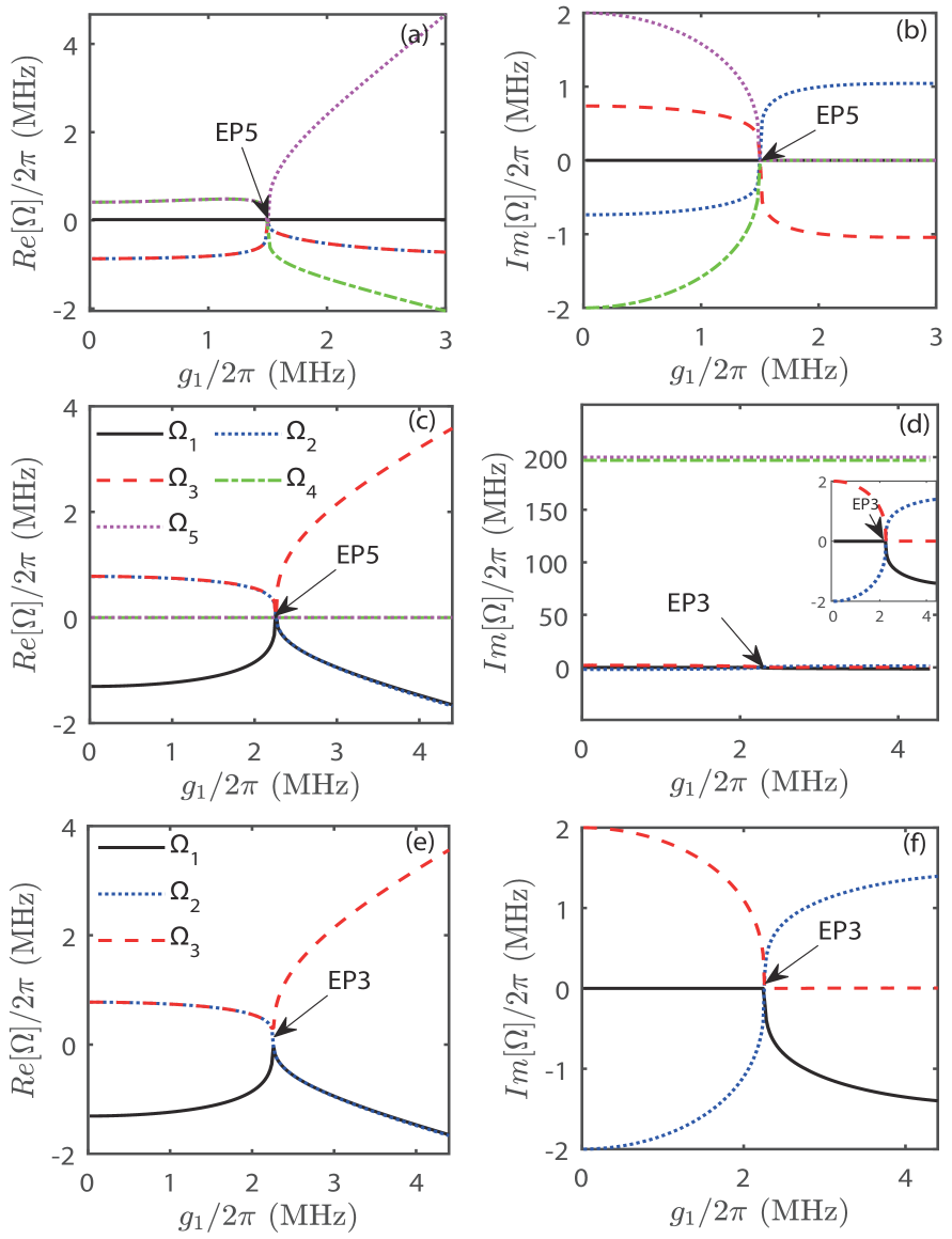
Figure 14: Comparison of the eigenvalue conversions from non-Markovian to Markovian regimes for EPs as a function of the coupling strength $g_{1}$ based on Eq. (64). (a) and (b) respectively plot the real and imaginary parts of the eigenvalues of the effective Hamiltonian $\hat{H}_{N5}$ in the non-Markovian case with $\lambda_{1}/2\pi=0.079$ MHz and $\lambda_{2}/2\pi=2.921$ MHz. (c) and (d) display the real and imaginary parts during the conversion to the Markovian regime, corresponding to $\lambda_{1}/2\pi=200$ MHz and $\lambda_{2}/2\pi=220$ MHz. (e) and (f) present the real and imaginary parts under the Markovian approximation. With other parameters fixed at $\gamma_{1}/2\pi=2$ MHz and $\gamma_{2}/2\pi=1$ MHz, the comparison demonstrates a change from a fifth-order exceptional point under pseudo-Hermitian conditions in different non-Markovian environments to a third-order exceptional point under the Markovian approximation.

In Fig. 14, we consider only the most general case where the dissipations of the cavity $b_{1}$ and cavity $b_{2}$ are different, which are denoted as $\gamma_{1}\neq\gamma_{2}$ (with $\gamma_{1}=2\gamma_{2}=2$ MHz as an example). Figure 14(a) and (b) respectively plot the real and imaginary parts of the eigenvalues as functions of $g_{1}$ in the non-Markovian case with the critical coupling strength ${g}_{\text{EP5}}=1.5$ MHz at EP. When $g_{1}<{g}_{\text{EP5}}$, the five eigenvalues manifest as one real and two pairs of complex conjugates. At $g_{1}={g}_{\text{EP5}}$ (i.e., at EP5), the five eigenvalues coalesce into a real number. When $g_{1}>{g}_{\text{EP5}}$, the eigenvalues appear as three reals and one pair of complex conjugates with the parameter $g_{2}=0.589$ MHz. Figure 14(c) and (d) show the real and imaginary parts of the eigenvalues as functions of $g_{1}$ during the conversion from non-Markovian to Markovian regimes. Comparing them with Fig. 14(e) and (f), the difference lies in the presence of two lines with real parts equalling to zero and imaginary parts representing the spectral widths of the non-Markovian environments ($\Omega_{4}$ and $\Omega_{5}$). In this case, the critical coupling strength is ${g}_{\text{EP3}}(g_{\text{EP5}})/2\pi=2.258$ MHz. When $g_{1}<{g}_{\text{EP3}}$, three eigenvalues are observed as one real and one pair of complex conjugates. At $g_{1}={g}_{\text{EP3}}$, i.e., at EP3, the three eigenvalues coalesce into a real number. When $g_{1}>{g}_{\text{EP3}}$, the eigenvalues appear as another real and one pair of complex conjugates. The remaining parameters are set to $g_{2}/2\pi=1.125$ MHz, $\Gamma_{1}/2\pi=4$ MHz, and $\Gamma_{2}/2\pi=2$ MHz. We can observe the conversion from a fifth-order exceptional point in a non-Markovian pseudo-Hermitian system to a third-order exceptional point in a Markovian system.

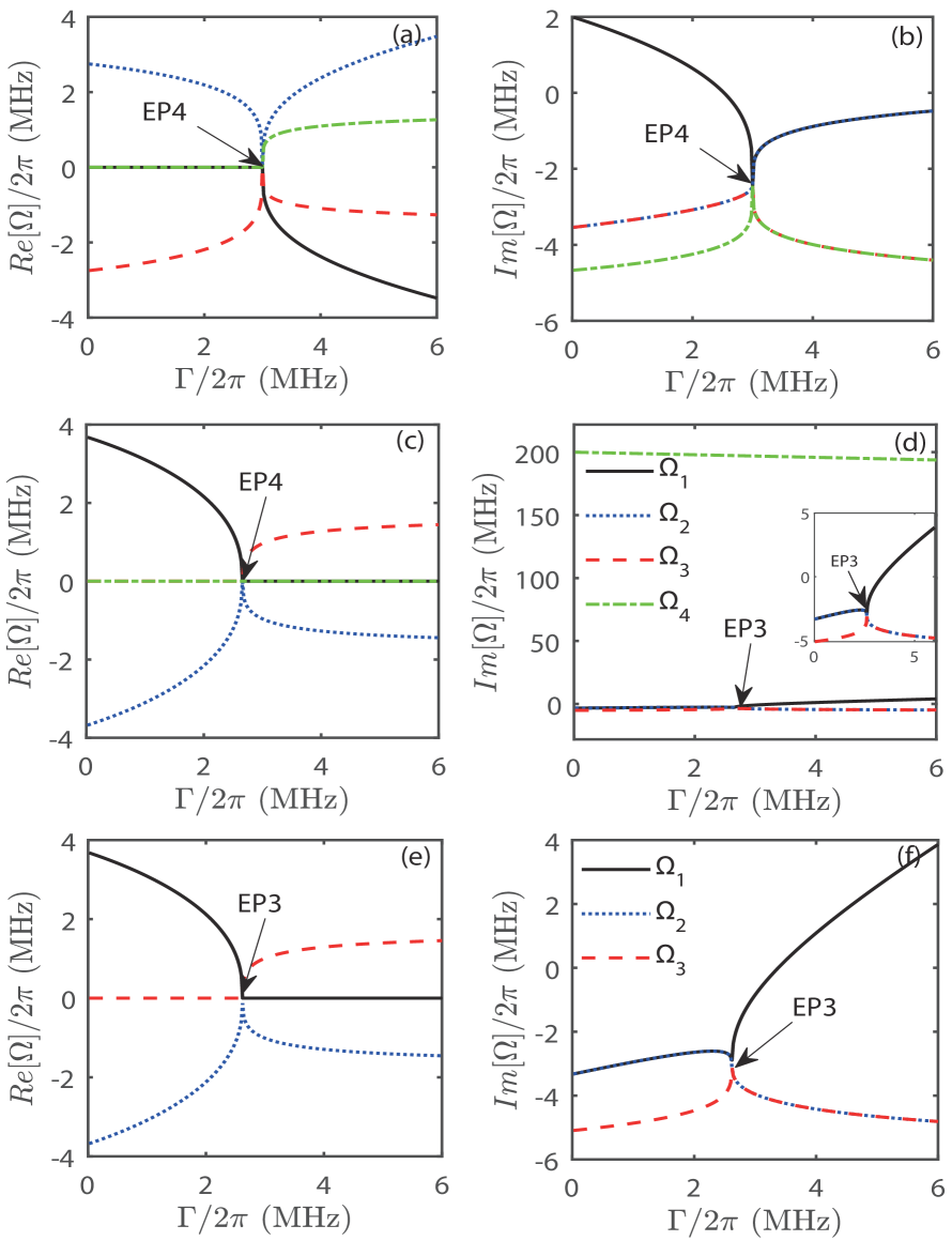
Figure 15: Under the symmetric case without considering the pseudo-Hermitian condition ($\gamma_{1}=\gamma_{2}$), a comparative analysis performs the eigenvalue evolution with respect to the dissipation $\Gamma$ between the non-Markovian and Markovian regimes based on Eq. (32). (a) and (b) show the real and imaginary parts of the eigenvalues of the effective Hamiltonian $\hat{H}_{\rm{NMeff}}$ in the non-Markovian case with $\lambda_{1}/2\pi=\lambda_{2}/2\pi=2$ MHz and $\Gamma/2\pi=3$ MHz. (c) and (d) plot the real and imaginary parts as it changes to the Markovian regime, where $\lambda_{1}/2\pi=\lambda_{2}/2\pi=200$ MHz and $\Gamma/2\pi=2.620$ MHz. (e) and (f) show the real and imaginary parts under the Markovian approximation. For all cases, the other parameters are set as $J/2\pi=1$ MHz and $\gamma_{1}/2\pi=\gamma_{2}/2\pi=5.880$ MHz.

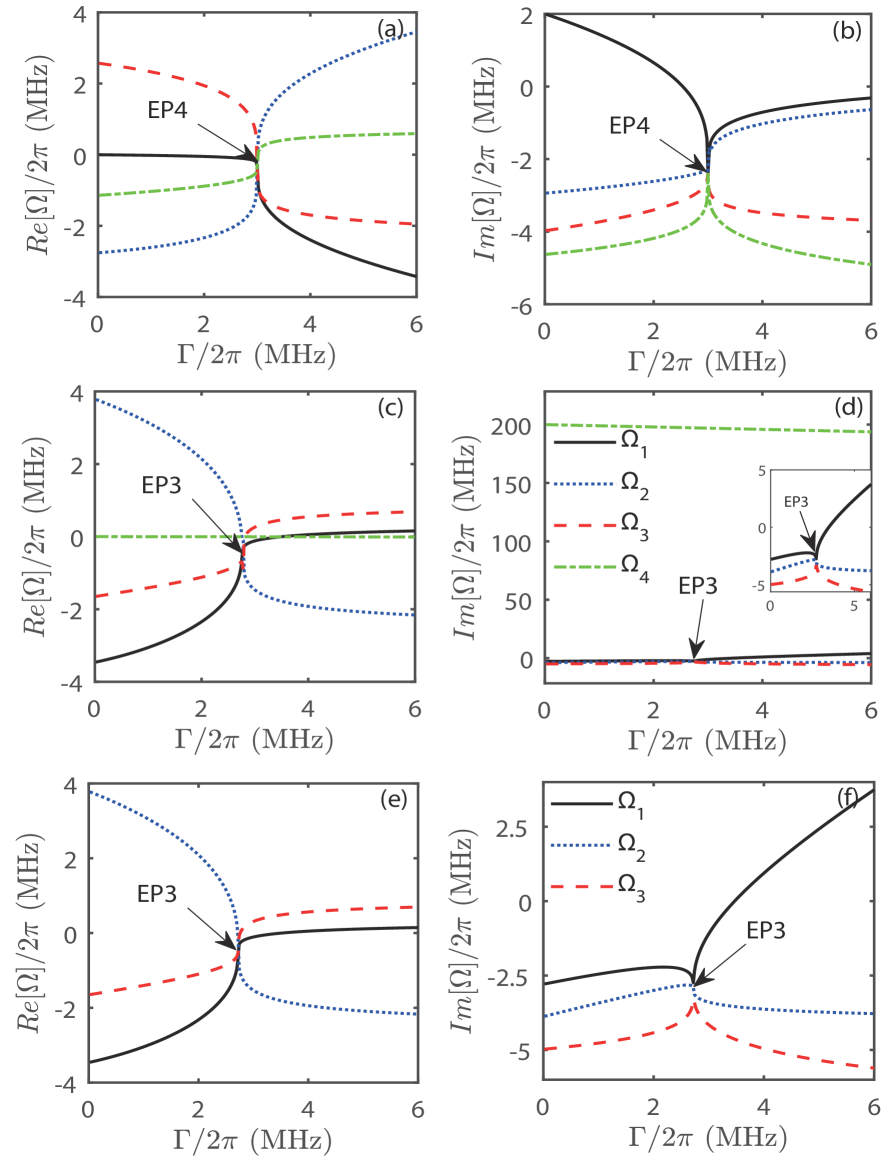
Figure 16: In the asymmetric case without considering the pseudo-Hermiticity condition (i.e., $\gamma_{1}\neq\gamma_{2}$, exemplified by $\gamma_{1}=2\gamma_{2}$), we discuss the eigenvalue variations with respect to the dissipation $\Gamma$ between the non-Markovian and Markovian regimes based on Eq. (32). (a) and (b) describe the real and imaginary parts of the eigenvalues of the effective Hamiltonian $\hat{H}_{\rm{NMeff}}$ in the non-Markovian case with $\lambda_{1}/2\pi=\lambda_{2}/2\pi=2$ MHz and $\Gamma/2\pi=3$ MHz. (c) and (d) show the real and imaginary parts as it changes to the Markovian regime, where $\lambda_{1}/2\pi=\lambda_{2}/2\pi=200$ MHz and $\Gamma/2\pi=2.723$ MHz. (e) and (f) represent the real and imaginary parts under the Markovian approximation. The remaining parameter is set as $J/2\pi=1$ MHz.

VII Expand to more general Non-Hermitian Situations in non-Markovian environments

Next, we will explore the extension of non-Hermitian exceptional points with pseudo-Hermiticity to the general non-Markovian non-Hermitian case, where the system does not need to consider the pseudo-Hermitian condition. The following discussions will be carried out in several cases:

VII.1 The fourth-order exceptional points

When the spectral widths of the non-Markovian environments at the two ports are equal, the effective non-Hermitian Hamiltonian can be expressed in the form of a fourth-order matrix in Eq. (47). Based on the discriminant of the roots for the quartic equation in Eq. (59), the following analysis can be performed.

$a$. When the dissipations of the two cavities are equal ($\gamma_{1}=\gamma_{2}$), the fourth-order non-Hermitian non-Markovian exceptional point can return to the third-order non-Hermitian Markovian exceptional point as the spectral width of the environment $\lambda$ tends to infinity.

$b$. When the dissipations of the two cavities are unequal $\gamma_{1}\neq\gamma_{2}$ (specifically, $\gamma_{1}=2\gamma_{2}$) and the spectral widths of the environments tend to infinity, the fourth-order non-Hermitian non-Markovian exceptional point similarly undergoes a conversion to the third-order non-Hermitian Markovian exceptional point. Now we have a detailed discussion.

Figure 15 presents higher-order EPs in the system where the dissipation rates of the two cavities $b_{1}$ and $b_{2}$ are equal ($\gamma_{1}=\gamma_{2}$). The four lines in Fig. 15(a) and (c) represent the variations of the real parts of four eigenvalues with respect to the coupling strength $g_{1}$, while Fig. 15(b) and (d) show the corresponding variations of their imaginary parts. Specifically, Fig. 15(a) and (b) describe a non-Hermitian fourth-order EP in the non-Markovian regime. Figure 15(c) and (d) present the conversion from the non-Markovian to Markovian regimes for an EP4. Figure 15(e) and (f) correspond to the real and imaginary parts of EP3 under the Markovian approximation. A conversion from the non-Markovian to Markovian regime is achievable. Different from the EPs presented earlier in the paper (e.g., Sec. II- Sec. VI), the parameters here do not need to satisfy pseudo-Hermitian conditions.

Figure 16 shows a case with significant dissipation differences, while the remaining detailed descriptions follow the same situation as Fig. 15. In contrast to Fig. 15, the real parts of the eigenvalues exhibit asymmetric features. By contrasting these three cases in Figs. 15 and 16, extending into the non-Hermitian regime enables a conversion from a fourth-order exceptional point in a non-Markovian environment to a third-order exceptional point under the Markovian approximation.

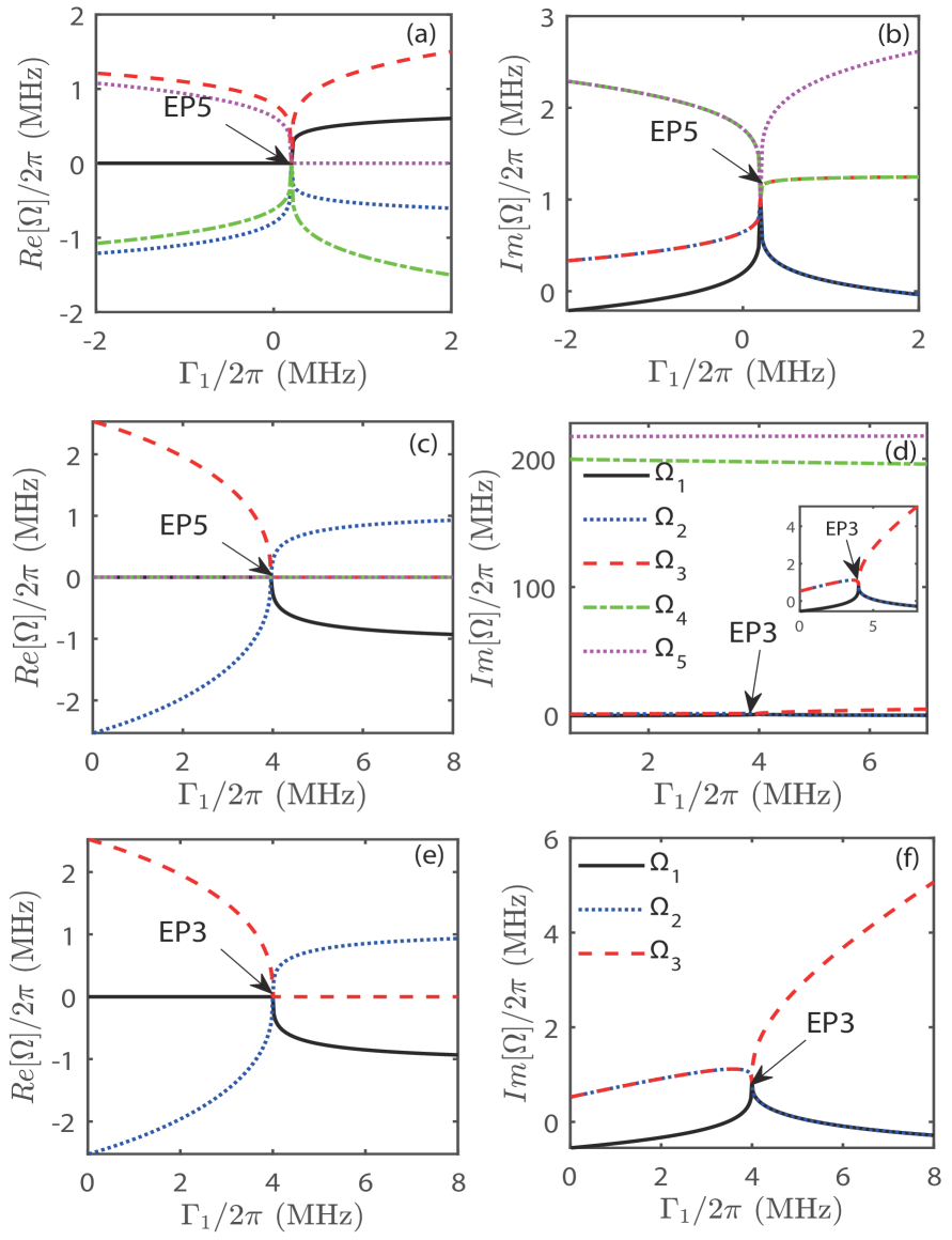
Figure 17: Under the symmetric condition ($\gamma_{1}=\gamma_{2}$) in non-Hermitian systems within different non-Markovian environments, the eigenvalues in the conversion from non-Markovian to Markovian regimes evolve with the dissipation $\Gamma_{1}$ based on Eq. (64). (a) and (b) respectively exhibit the real and imaginary parts of the eigenvalues of the effective Hamiltonian $\hat{H}_{N5}$ in the non-Markovian case with $\lambda_{1}/2\pi=0.2$ MHz, $\lambda_{2}/2\pi=6.828$ MHz, $\Gamma_{1}/2\pi=0.2$ MHz, and $\Gamma_{2}/2\pi=4.739$ MHz. (c) and (d) respectively correspond to the real and imaginary parts during the conversion to the Markovian regime with $\lambda_{1}/2\pi=200$ MHz, $\lambda_{2}/2\pi=220$ MHz, $\Gamma_{1}/2\pi=4$ MHz, and $\Gamma_{2}/2\pi=5$ MHz. (e) and (f) describe the real and imaginary parts under the same parameters. The remaining parameters are set as $J/2\pi=1$ MHz and $\gamma_{2}/2\pi=1$ MHz.

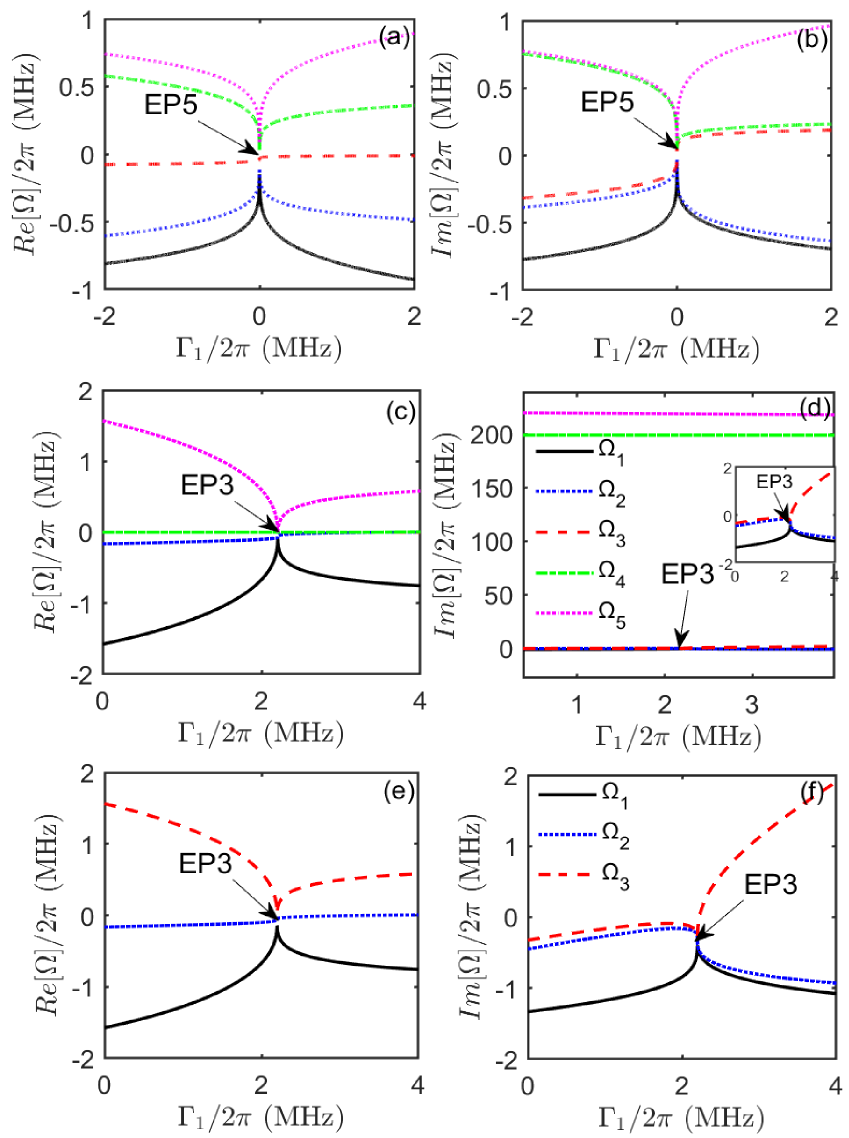
Figure 18: In the asymmetric case ($\gamma_{1}\neq\gamma_{2}$) within non-Hermitian systems with non-Markovian environments, the conversion to the Markovian regime and the variation of eigenvalues with the dissipation $\Gamma_{1}$ are plotted based on Eq. (64). (a) and (b) respectively exhibit the real and imaginary parts of these eigenvalues with $\lambda_{1}/2\pi=3$ MHz, $\lambda_{2}/2\pi=0.056$ MHz, $\Gamma_{1}/2\pi=2.558$ MHz, and $\Gamma_{2}/2\pi=2.158\times 10^{-6}$ MHz. (c) and (d) respectively present the real and imaginary parts during the conversion to Markovian regime with $\lambda_{1}/2\pi=200$ MHz, $\lambda_{2}/2\pi=220$ MHz, $\Gamma_{1}/2\pi=1.8$ MHz, and $\Gamma_{2}/2\pi=2.2$ MHz. (e) and (f) respectively describe the real and imaginary parts under the same set of parameters. For all cases, the other parameters are set as $J/2\pi=1$ MHz, $\gamma_{1}/2\pi=1$ MHz, and $\gamma_{2}/2\pi=2$ MHz.

VII.2 The fifth-order exceptional points

For the different spectral widths of the non-Markovian environments at the two different ports, the effective non-Hermitian Hamiltonian can be denoted as a fifth-order matrix in Eq. (64). With the discriminant of the roots of the quintic equation in Eq. (66), the detail analysis can be carried out.

$a$. As $\lambda_{1}=\lambda_{2}\to\infty$ with $\gamma_{1}=\gamma_{2}$, the fifth-order exceptional point in Fig. 17 emerges and experiences a conversion to a third-order exceptional point.

$b$. For the case with $\gamma_{1}\neq\gamma_{2}$ in Fig. 18, there are similar phenomena compared to the previous discussions.

Figure 17 explores a conversion process within a system where the two non-Markovian environmental spectral widths of the cavity $a$ are different ($\lambda_{1}\neq\lambda_{2}$), specifically the conversion from a fifth-order non-Markovian exceptional point to a third-order Markovian exceptional point occurs when the dissipations of the two cavities ($b_{1}$ and $b_{2}$) are the same (i.e., $\gamma_{1}=\gamma_{2}$). The analysis of this process follows the same method previously described with the aim of uncovering profound insights into the dynamics of the system.

Figure 18 presents the conversion from a fifth-order non-Markovian exceptional point to a third-order Markovian exceptional point in the system with unequal dissipation rates ($\gamma_{1}=2\gamma_{2}$) between the two cavities ($b_{1}$ and $b_{2}$) under different environmental spectral widths ($\lambda_{1}$ and $\lambda_{2}$). Due to the non-Markovian effect, the memory effects of environments to the system cause the dynamical behavior no longer dependent on the current state but also influenced by past states. As a result, phenomena such as branching, merging, or crossing may emerge in the real part Tschernig2022 , which are manifestations of the unique non-Markovian regimes in non-Hermitian systems. The variation in the imaginary part reflects the characteristics of system dissipation and oscillation behavior. In the non-Markovian environments owing to the memory effect, the imaginary part may no longer maintain a simple linear or constant value but fluctuate with changes in $g_{1}$, indicating complex variations in the system’s dissipative properties. As the system converts from non-Markovian to Markovian regimes, the real part’s variation may gradually smoothen with less branching or crossing phenomena, ultimately tending towards the behavioral patterns observed under the Markovian approximation, where the absence of memory effects simplifies the dynamical behavior.

VIII Sixth-order and Seventh-order Exceptional Points

In this section, we consider that the environments of the two ports of the cavity $a$ are in non-Markovian regimes, and so are the environments of the cavities $b_{1}$ and $b_{2}$, where the environments are composed of a series of bosonic modes. The cavity is coupled to the $k$th mode (eigenfrequency $\alpha_{k}$ and $\beta_{k}$) of the non-Markovian environments via the annihilation (creation) operators $\hat{e}_{k}(\hat{e}^{{\dagger}}_{k})$ and $\hat{f}_{k}(\hat{f}^{{\dagger}}_{k})$. The total non-Markovian Hamiltonian with Eq. (32) is changed to

$$\hat{H}_{NM}^{\prime} =\ \omega_{c}\hat{a}^{\dagger}\hat{a}+\sum_{j=1,2}\left[\omega_{j}\hat{b}_{j}^{\dagger}\hat{b}_{j}+g_{j}(\hat{a}^{\dagger}b_{j}+\hat{a}\hat{b}_{j}^{\dagger})\right]$$

$$+J(\hat{b}_{1}^{\dagger}\hat{b}_{2}+\hat{b}_{1}\hat{b}_{2}^{\dagger})+\sum_{k}\omega_{k}\hat{c}_{k}^{\dagger}\hat{c}_{k}+\sum_{k}\Omega_{k}\hat{d}_{k}^{\dagger}\hat{d}_{k}$$

$$+\sum_{k}\alpha_{k}\hat{e}_{k}^{\dagger}\hat{e}_{k}+\sum_{k}\beta_{k}\hat{f}_{k}^{\dagger}\hat{f}_{k}+i\sum_{k}(g_{k}\hat{a}\hat{c}_{k}^{\dagger}-g_{k}^{*}\hat{a}^{\dagger}\hat{c}_{k})$$

$$+i\sum_{k}(G_{k}\hat{a}\hat{d}_{k}^{\dagger}-G_{k}^{*}\hat{a}^{\dagger}\hat{d}_{k})+i\sum_{k}(A_{k}\hat{b}_{1}\hat{e}_{k}^{\dagger}-A_{k}^{*}\hat{b}_{1}^{\dagger}\hat{e}_{k})$$

$$+i\sum_{k}(B_{k}\hat{b}_{2}\hat{f}_{k}^{\dagger}-B_{k}^{*}\hat{b}_{2}^{\dagger}\hat{f}_{k}),$$ (71)

where $g_{k}$, $G_{k}$, $A_{k}$, and $B_{k}$ respectively denote the interaction strengths between the two ports 1, 2 of the cavity $a$, the cavity $b_{1}$, the cavity $b_{2}$ and the surrounding non-Markovian environments with intrinsic frequencies $\omega_{k}$, $\Omega_{k}$, $\alpha_{k}$, $\beta_{k}$. With Eq. (71), the Heisenberg equation reads

$$\frac{d}{dt}\hat{a}(t)= -i\omega_{c}\hat{a}(t)-ig_{1}\hat{b_{1}}(t)-ig_{2}\hat{b}_{2}(t)-\sum_{k}g_{k}^{*}\hat{c}_{k}(t)$$

$$-\sum_{k}G_{k}^{*}\hat{d}_{k}(t),$$

$$\frac{d}{dt}\hat{b}_{1}(t)= -i\omega_{1}\hat{b}_{1}(t)-ig_{1}\hat{a}(t)-iJ\hat{b_{2}}(t)-\sum_{k}A_{k}^{*}\hat{e}_{k}(t),$$

$$\frac{d}{dt}\hat{b}_{2}(t)= -i\omega_{2}\hat{b}_{2}(t)-ig_{2}\hat{a}(t)-iJ\hat{b_{1}}(t)-\sum_{k}B_{k}^{*}\hat{f}_{k}(t),$$

$$\frac{d}{dt}\hat{c}_{k}(t)= -i\omega_{k}\hat{c}_{k}(t)+g_{k}\hat{a}(t),$$

$$\frac{d}{dt}\hat{d}_{k}(t)= -i\Omega_{k}\hat{d}_{k}(t)+G_{k}\hat{a}(t),$$

$$\frac{d}{dt}\hat{e}_{k}(t)= -i\alpha_{k}\hat{e}_{k}(t)+A_{k}\hat{b}_{1}(t),$$

$$\frac{d}{dt}\hat{f}_{k}(t)= -i\beta_{k}\hat{f}_{k}(t)+B_{k}\hat{b}_{2}(t).$$ (72)

The environmental operators are derived by solving Eq. (72)

$$\hat{c}_{k}(t) =\hat{c}_{k}(0)e^{-i\omega_{k}t}+g_{k}\int_{0}^{t}\hat{a}(\tau)e^{-i\omega_{k}(t-\tau)}d\tau,$$ (73)

$$\hat{d}_{k}(t) =\hat{d}_{k}(0)e^{-i\Omega_{k}t}+G_{k}\int_{0}^{t}\hat{a}(\tau)e^{-i\Omega_{k}(t-\tau)}d\tau,$$

$$\hat{e}_{k}(t) =\hat{e}_{k}(0)e^{-i\alpha_{k}t}+A_{k}\int_{0}^{t}\hat{b}_{1}(\tau)e^{-i\alpha_{k}(t-\tau)}d\tau,$$

$$\hat{f}_{k}(t) =\hat{f}_{k}(0)e^{-i\beta_{k}t}+B_{k}\int_{0}^{t}\hat{b}_{2}(\tau)e^{-i\beta_{k}(t-\tau)}d\tau,$$

where the first term reflects the free evolution of the non-Markovian environmental fields, while the second term captures the non-Markovian feedback effects from the environments onto the cavities. By substituting Eq. (73) into Eq. (72), we derive the non-Markovian Heisenberg-Langevin equation for the cavity operators

$$\frac{d}{dt}\hat{a}(t)= -i\omega_{c}\hat{a}(t)-ig_{1}\hat{b}_{1}(t)-ig_{2}\hat{b}_{2}(t)+\hat{K}_{1}(t)+\hat{K}_{2}(t)$$

$$-\int_{0}^{t}\hat{a}(\tau)f_{1}(t-\tau)d\tau-\int_{0}^{t}\hat{a}(\tau)f_{2}(t-\tau)d\tau,$$

$$\frac{d}{dt}\hat{b}_{1}(t)= -i\omega_{1}\hat{b}_{1}(t)-ig_{1}\hat{a}(t)-iJ\hat{b_{2}}(t)+\hat{K}_{3}(t)$$

$$-\int_{0}^{t}\hat{b}_{1}(\tau)f_{3}(t-\tau)d\tau,$$

$$\frac{d}{dt}\hat{b}_{2}(t)= -i\omega_{2}\hat{b}_{2}(t)-ig_{2}\hat{a}(t)-iJ\hat{b_{1}}(t)+\hat{K}_{4}(t)$$

$$-\int_{0}^{t}\hat{b}_{2}(\tau)f_{4}(t-\tau)d\tau,$$ (74)

where

$$\hat{K}_{3}(t)=-\sum_{k}A_{k}^{*}\hat{e}_{k}(0)e^{-i\alpha_{k}t}=\int_{-\infty}^{\infty}\kappa^{*}_{3}(t-\tau)\hat{b}^{(in)}_{1}(\tau)d\tau,$$

$$\hat{K}_{4}(t)=-\sum_{k}B_{k}^{*}\hat{f}_{k}(0)e^{-i\beta_{k}t}=\int_{-\infty}^{\infty}\kappa^{*}_{4}(t-\tau)\hat{b}^{(in)}_{2}(\tau)d\tau,$$

$$\hat{b}^{(in)}_{1}(t)=-\frac{1}{\sqrt{2\pi}}\sum_{k}\hat{e}_{k}(0)e^{-i\alpha_{k}t},$$

$$\hat{b}^{(in)}_{2}(t)=-\frac{1}{\sqrt{2\pi}}\sum_{k}\hat{f}_{k}(0)e^{-i\beta_{k}t},$$

$$\kappa_{3}(t-\tau)=\frac{1}{\sqrt{2\pi}}\int e^{i\omega(t-\tau)}A(\omega)d\omega,$$

$$\kappa_{4}(t-\tau)=\frac{1}{\sqrt{2\pi}}\int e^{i\omega(t-\tau)}B(\omega)d\omega,$$

$$f_{3}(t)=\int J_{3}(\omega)e^{-i\omega t}d\omega,\ f_{4}(t)=\int J_{4}(\omega)e^{-i\omega t}d\omega,$$

$$J_{3}(\omega)=\sum_{k}|A_{k}|^{2}\delta(\omega-\alpha_{k}),$$ (75)

and $J_{4}(\omega)=\sum_{k}|B_{k}|^{2}\delta(\omega-\beta_{k})$. Eq. (74) can be written as a matrix form with $\mathbf{N}=(\hat{a},\hat{b}_{1},\hat{b}_{2},\hat{Z}_{1},\hat{Z}_{2},\hat{Z}_{3},\hat{Z}_{4})^{T}$

$$\dot{\mathbf{N}}=-i\hat{H}_{N7}\mathbf{N},$$ (76)

where we have used the non-Markovian input-output relations in Eq. (42) and defined $\hat{b}_{1}^{(out)}(t)+\hat{b}_{1}^{(in)}(t)=\int_{0}^{t}\kappa_{3}(\tau-t)\hat{b}_{1}(\tau)d\tau$, $\hat{b}_{2}^{(out)}(t)+\hat{b}_{2}^{(in)}(t)=\int_{0}^{t}\kappa_{4}(\tau-t)\hat{b}_{2}(\tau)d\tau$ as well as imposing CPA. $\hat{H}_{N7}$ in Eq. (76) denotes the non-Markovian system’s effective non-Hermitian Hamiltonian

$$\hat{H}_{N7}=\begin{pmatrix}\omega_{c}&g_{1}&g_{2}&-i\mu_{1}&-i\mu_{2}&0&0\\ g_{1}&\omega_{1}-i\gamma_{1}&J&0&0&i\mu_{3}&0\\ g_{2}&J&\omega_{2}-i\gamma_{2}&0&0&0&i\mu_{4}\\ i\mu_{1}&0&0&i\lambda_{1}&0&0&0\\ i\mu_{2}&0&0&0&i\lambda_{2}&0&0\\ 0&i\mu_{3}&0&0&0&i\lambda_{3}&0\\ 0&0&i\mu_{4}&0&0&0&i\lambda_{4}\end{pmatrix},$$ (77)

where $\mu_{n}\equiv\sqrt{{\lambda_{n}\Gamma_{n}}/{2}}$ ($n=1,2,3,4$).

When the two non-Markovian environments coupling with the cavity $a$ are identical (i.e., $\mu_{2}=\mu_{1}$), the non-Markovian effective Hamiltonian in Eq. (77) can be reduced to

$$\hat{H}_{N6}=\begin{pmatrix}\omega_{c}&g_{1}&g_{2}&-2i\mu_{1}&0&0\\ g_{1}&\omega_{1}-i\gamma_{1}&J&0&i\mu_{3}&0\\ g_{2}&J&\omega_{2}-i\gamma_{2}&0&0&i\mu_{4}\\ i\mu_{1}&0&0&i\lambda_{1}&0&0\\ 0&i\mu_{3}&0&0&i\lambda_{3}&0\\ 0&0&i\mu_{4}&0&0&i\lambda_{4}\end{pmatrix}.$$ (78)

Based on the Hamiltonians provided by Eqs. (77) and (78), we can investigate the properties of higher-order exceptional points (EP6 for $\hat{H}_{N6}$ and EP7 for $\hat{H}_{N7}$) within non-Markovian environments. The method employed can be similar to the previous sections, which holds significant values for advancing the understanding of higher-order exceptional points in non-Markovian systems. Here, we will not go into detailed discussions.

IX conclusion

Before drawing our conclusions, let us evaluate the practical feasibility of implementing our proposal within SC circuit systems. Specifically, the SC cavity can obtain a characteristic frequency range of 1 GHz to 10 GHz in experimental settings, accompanied by a loss rate in the vicinity of 0.1 MHz to 1 MHz Gu12017 . The integration of a superconducting quantum interference device (SQUID) within the SC cavity allows for easier adjustment of its frequency, achieved through controlling the bias agnetic flux threading the SQUID loop Partanen5052019 . For the case of an active SC cavity, the capability to fine-tune its gain rate, spanning from 0 MHz to 6 MHz, is achievable by regulating the driving fields applied to an auxiliary SC qubit that transversely interacts with the cavity Zhang2022020 . Moreover, experimental demonstrations have verified the tunable coupling strength between SC cavities, varying from 0.62 MHz to 16 MHz, Baust5152015 . Given these viable technological advancements, the experimental realization of our proposal stands as a feasible endeavor.

To summarize, we have studied higher-order EPs within the system composed of three coupled cavities with balanced gain and loss. Under specific parameters conditions, the system’s effective Hamiltonian exhibits pseudo-Hermiticity, manifesting in its eigenvalue structure as either three real eigenvalues or a single real eigenvalue accompanied by a pair of complex-conjugate eigenvalues. Through precise modulation of the coupling strength $g_{1}$ between cavities, particularly between the cavities $a$ and $b_{1}$, we observe the coalescence of three eigenvalues into an EP3 within the system’s parameter space. Moreover, our theory suggests that the pseudo-Hermiticity and EP3 of the proposed system can be probed through the total output spectrum characterizing the system’s input-output properties.

Moreover, we broaden our research range by examining the effects of introducing identical and different non-Markovian environments to the cavity $a$. Within the parameter space that preserves the system’s pseudo-Hermiticity, by tuning the coupling strength $g_{1}$ between the cavities $a$ and $b_{1}$, we observe even more complex phenomena, including the emergence of EP4 with four eigenvalues coalescing and EP5 with five eigenvalues merging. We expand our perspective from pseudo-Hermiticity to more general non-Hermitian systems, showing how EPs change through a conversion from non-Markovian to Markovian regimes as system parameters vary.

Finally, we discuss the higher-order exceptional points (i.e., EP6 and EP7) when all three cavities are immersed in different non-Markovian environments. This implies that the study of higher-order EPs in non-Hermitian systems with non-Markovian conditions will open up new theoretical and application areas. The results not only deepens our understanding of the dynamical behaviors in non-Hermitian systems but also offers fresh insights into the application in non-Markovian open quantum systems.

As a future perspective, it is of significant interest to conduct an indepth investigation into the total excitation number being non-conservative systems without the rotating-wave approximation. For example, one can explore the non-rotating-wave interaction between a cavity and the environment mathematically formulated as $\sum_{m}I_{m}(\hat{b}+\hat{b}^{\dagger})(\hat{d}_{m}+\hat{d}_{m}^{\dagger})$ Shen7072022 ; Shen042121 ; Shen0338052017 ; Shen0238562018 ; Shen013826 . In fact, the Hamiltonian with all couplings between different subsystems may have the anisotropic non-rotating wave form $\sum_{p,m}(F_{p,m}\hat{U}_{p}\hat{V}_{m}^{\dagger}+F_{p,m}^{*}\hat{U}_{p}^{\dagger}\hat{V}_{m}+K_{p,m}\hat{U}_{p}\hat{V}_{m}+K_{p,m}^{*}\hat{U}_{p}^{\dagger}\hat{V}_{m}^{\dagger})$ Xie0210462014 ; Chen0437082021 ; Rodriguez0466082008 ; Nakajima3631955 ; Ai042116 ; Zheng559 ; Frohlich8451950 ; Frohlich2911952 ; Lu0543022007 ; Fischer1604012016 ; Overbeck0121062016 ; Medvedyeva0942052016 ; Metcalf0232142020 ; Xu0121062019 ; Lebreuilly0338282017 , where $\hat{U}_{p}^{\dagger}$ ($\hat{U}_{p}$) and $\hat{V}_{m}^{\dagger}$ ($\hat{V}_{m}$) are the creation (annihilation) operators for the whole system, while $F_{p,m}$ and $K_{p,m}$ respectively denote the coupling strengths of the rotating-wave and non-rotating-wave interactions.

Appendix A The impulse response functions $\kappa_{\nu}(t)$ and correlation function $f_{\nu}(t)$ can be realized through the pseudomode theory

Taking a cavity mode as an example exhibits the controllability of Lorentzian spectrum density in non-Markovian environments by applying Markovian pseudomodes method Jack0438032001 ; Barnett1997 ; Garraway5522901997 ; Garraway5546361997 ; Man900621042014 ; Man2357632015 ; Mazzola800121042009 ; Pleasance960621052017 . We introduce a system consisting of a cavity mode (eigenfrequency ${\omega_{n}}$) interacting with a pseudomode (eigenfrequency $\omega_{x}$), whose Hamiltonian is

$${{\hat{H}}_{S}}={\omega_{n}}{{\hat{n}}^{\dagger}}\hat{n}+{\omega_{x}}{{\hat{x}}^{\dagger}}\hat{x}+{g_{nx}}(\hat{n}{{\hat{x}}^{\dagger}}+{{\hat{n}}^{\dagger}}\hat{x}),$$ (79)

where the first and second terms on the right-hand side describe the free Hamiltonian with the cavity annihilation operator $\hat{n}$ and pseudomode annihilation operator $\hat{x}$, which satisfy the bosonic commutation relations $[\hat{n},{\hat{n}}^{\dagger}]=1$ and $[\hat{x},{\hat{x}}^{\dagger}]=1$. The last term in Eq. (79) corresponds to the tunneling coupling between cavity mode and pseudomode with the coupling strength ${g_{nx}}$. The corresponding total Hamiltonian including the Markovian environment reads

$${{\hat{H}_{T}}}={{\hat{H}}_{S}}+{{\hat{H}}_{R}}+{{\hat{H}}_{I}},$$ (80)

where ${{\hat{H}}_{I}}=i\sum\nolimits_{k}{{V_{k}}}(\hat{q}_{k}^{\dagger}\hat{x}-{{\hat{x}}^{\dagger}}{{\hat{q}}_{k}})$ (interaction Hamiltonian between pseudomode and Markovian environment with coupling strength ${V_{k}}=\sqrt{\gamma/2\pi}$ and decay rate $\gamma$), ${\hat{H}_{R}}=\sum\nolimits_{k}{{\omega_{k}}\hat{q}_{k}^{\dagger}{\hat{q}_{k}}}$ (free Hamiltonian of Markovian environment) with $[{\hat{q}_{k}},\hat{q}_{k^{\prime}}^{\dagger}]={\delta_{kk^{\prime}}}$. With Eq. (80), the Heisenberg-Langevin equations under the Markovian approximation are GardinerBerlin2000 ; Walls1994

$$\frac{d}{{dt}}\hat{n} = -i{\omega_{n}}\hat{n}-i{g_{nz}}\hat{x},$$ (81)

$$\frac{d}{{dt}}\hat{x} = -i{g_{nx}}\hat{n}-\frac{\gamma}{2}\hat{x}-\sqrt{\gamma}{{\hat{q}}_{in}}(t).$$ (82)

Solving Eq. (82) for $\hat{x}\left(t\right)$ gets $\hat{x}(t)=\hat{x}(0){e^{-\frac{\gamma}{2}t}}-i{g_{nx}}\int_{0}^{t}{\hat{n}(\tau){e^{-\frac{\gamma}{2}(t-\tau)}}d\tau}-\sqrt{\gamma}\int_{0}^{t}{{{\hat{q}}_{in}}(\tau){e^{-\frac{\gamma}{2}(t-\tau)}}d\tau}$ with ${\hat{q}_{{\rm{in}}}}(t){\rm{=}}\sum\nolimits_{k}{{e^{-i{\omega_{k}}t}}}{\hat{q}_{k}}/\sqrt{2\pi}$. Substituting $\hat{x}(t)$ into Eq. (81), we obtain

$$\frac{d}{{dt}}\hat{n}=-i{\omega_{n}}\hat{n}-\int_{0}^{t}{\beta(t-\tau)\hat{n}(\tau)d\tau}-\hat{R}(t),$$ (83)

where the operator for the non-Markovian composite environment (including pseudomode plus its Markovian environment) $\hat{R}(t)=i{g_{nx}}\hat{x}(0){e^{-\frac{\gamma}{2}t}}-i{g_{nx}}\sqrt{\gamma}\int_{0}^{t}{{{\hat{q}}_{in}}(\tau){e^{-\frac{\gamma}{2}(t-\tau)}}d\tau}$ and correlation function $\beta(t)=g_{nx}^{2}{e^{-\frac{\gamma}{2}t}}$. The Lorentzian spectrum density $J(\omega)$ corresponding to the correlation function $\beta(t)=g_{nx}^{2}{e^{-\frac{\gamma}{2}t}}\equiv\int{J(\omega)}{e^{-i\omega t}}d\omega$ in Eq. (83) is equal to Eq. (44), where

$$\lambda_{\nu}=\gamma/2,\Gamma_{\nu}=4g_{nx}^{2}/\gamma,$$ (84)

which leads to

$$\beta(t-\tau)=\frac{1}{2}\Gamma_{\nu}\lambda_{\nu}e^{-\lambda_{\nu}(t-\tau)},$$ (85)

which is consistent with $f_{\nu}(t)$ below Eq. (44). With the operators expectation values defined by $n\equiv\left\langle\hat{n}\right\rangle$, $x\equiv\langle\hat{x}\rangle$, $q_{k}\equiv\langle\hat{q}_{k}\rangle$, $q_{in}\equiv\langle\hat{q}_{in}\rangle$, $R(t)\equiv\langle\hat{R}(t)\rangle$, $a_{in}\equiv\langle\hat{a}_{in}\rangle$, $K(t)\equiv\langle\hat{K}(t)\rangle$, $c\equiv\left\langle\hat{c}\right\rangle$ and considering the equality

$$K(t)\equiv-R(t),$$ (86)

we can obtain

$$q_{in}(t) =\frac{\gamma}{2}c(t)+c^{\prime}(t),$$ (87)

$$x=\frac{i}{g_{nx}}\int_{-\infty}^{+\infty}h^{*}(-\tau)a_{in}(\tau)d\tau,$$ (88)

with

$$c(t)=\frac{{{g_{nx}}x{e^{-\frac{\gamma}{2}t}}-iK(t)}}{{{g_{nx}}\sqrt{\gamma}}},$$ (89)

$$K(t)=\int_{-\infty}^{+\infty}h^{*}(t-\tau)a_{in}(\tau)d\tau.$$ (90)

The value of $x=\mathrm{Tr}[\hat{x}(0)\rho_{x}(0)]$ is determined by the initial state $\rho_{x}(0)$ of the pseudomode. If $x$ takes

$$x=i\frac{\sqrt{\Gamma}\lambda}{g_{nx}}\int_{0}^{+\infty}e^{-\lambda\tau}a_{in}(\tau)d\tau,$$ (91)

then comparing Eq. (88) and Eq. (91), we can get

$$h(t)=\sqrt{\Gamma}\lambda e^{\lambda t}\theta(-t),$$ (92)

which corresponds to $\kappa_{\nu}(t)$ above Eq. (43). $\hat{n}$ can represents $\hat{a}$, $\hat{b_{1}}$, and $\hat{b_{2}}$ in Eq. (35), which hold true according to Eq. (92). Therefore, when Eqs. (85), (87), (88), and (91) are satisfied simultaneously, we can verify that equations obtained by applying the Markovian pseudomode method are completely consistent with Eq. (35) in the non-Markovian regime.

Appendix B DERIVATION OF EQ. (47)

When CPA occurs $\hat{a}_{\nu}^{(out)}(t)=0$, using the non-Markovian input-output relationship derived from Eq. (42), we can obtain

$$\hat{a}_{\nu}^{(in)}(t)=\int_{0}^{t}\kappa_{\nu}(\tau-t)\hat{a}(\tau)d\tau.$$ (93)

To ensure the equations being closed, we define $2g\hat{X}(t)\equiv 2\hat{K}^{\dagger}(t)-2\int_{0}^{t}\hat{a}(\tau)f(t-\tau)d\tau$ in Eq. (46) with $g\equiv\sqrt{{\lambda\Gamma}/{2}}$, which leads to

$$\frac{d}{dt}\hat{X}(t)=\lambda\hat{X}(t)-g\hat{a}(t).$$ (94)

In this case, Eq. (46) becomes

$$\frac{d}{dt}\hat{a}(t)= -i\Delta_{c}\hat{a}(t)-ig_{1}\hat{b_{1}}(t)-ig_{2}\hat{b}_{2}(t)+2g\hat{X}(t),$$ (95)

$$\frac{d}{dt}\hat{b}_{1}(t)= -i(\Delta_{1}-i\gamma_{1})\hat{b}_{1}(t)-ig_{1}\hat{a}(t)-iJ\hat{b_{2}}(t),$$

$$\frac{d}{dt}\hat{b}_{2}(t)= -i(\Delta_{2}-i\gamma_{2})\hat{b}_{2}(t)-ig_{2}\hat{a}(t)-iJ\hat{b_{1}}(t),$$

$$\frac{d}{dt}\hat{X}(t)= \ \lambda\hat{X}(t)-g\hat{a}(t).$$

With $\mathbf{V_{1}}=(\hat{a},\hat{b}_{1},\hat{b}_{2},\hat{X})^{T}$, Eq. (95) is written as

$$\dot{\mathbf{V_{1}}}=-i\hat{H}_{NMeff}\mathbf{V_{1}},$$ (96)

where $\hat{H}_{\rm{NMeff}}$ is given by Eq. (47).

Appendix C Discussions on the inhomogeneous term in EQ. (48)

Our goal is to evaluate the impacts of the non-homogeneous terms ${a}_{in}^{(1)}(i{\lambda_{1}})$ and ${a}_{in}^{(2)}(i{\lambda_{2}})$ in Eq. (48). Taking $\hat{a}_{in}^{(1)}(t)$ as an illustrative example, we set $\phi({\lambda_{1}},\omega)={a}_{in}^{(1)}(i{\lambda_{1}})/{a}_{in}^{(1)}(\omega)$. The input field can take two different forms: a damped-oscillation form expressed as $\hat{a}_{in}^{(1)}(t)={x}{{\rm e}^{-zt}}\sin({y}{t^{2}})$ with $z>0$ and ${y}>0$, and a Gaussian-profile form given by $\hat{a}_{in}^{(1)}(t)={x}{{\rm e}^{-zt^{2}}}\cos({y}{t})$. These two forms respectively can give concrete expressions for $\phi({\lambda_{1}},\omega)$. For the damped-oscillation form, $\phi({\lambda_{1}},\omega)=\{\cos[\frac{{{{\left({\lambda+z}\right)}^{2}}}}{{4y}}][1-2fc(\frac{{\lambda+z}}{{\sqrt{2\pi y}}})]+[1-2fs(\frac{{\lambda+z}}{{\sqrt{2\pi y}}})]\sin[\frac{{{{\left({\lambda+z}\right)}^{2}}}}{{4y}}]\}/\{\cos[\frac{{{{\left({z-{\rm{i}}\omega}\right)}^{2}}}}{{4y}}][1-2fc(\frac{{z-{\rm{i}}\omega}}{{\sqrt{2\pi y}}})]+[1-2fs(\frac{{z-{\rm{i}}\omega}}{{\sqrt{2\pi y}}})]\sin[\frac{{{{\left({z-{\rm{i}}\omega}\right)}^{2}}}}{{4y}}]\}$. For the Gaussian - profile form, $\phi({\lambda_{1}},\omega)={e^{\frac{{{\lambda^{2}}+{\omega^{2}}+2y(\omega-i\lambda)}}{{4z}}}}\{i+{e^{\frac{{{\rm{i}}y\lambda}}{z}}}[i+erfi(\frac{{y-{\rm{i}}\lambda}}{{2\sqrt{z}}})]-erfi(\frac{{y+{\rm{i}}\lambda}}{{2\sqrt{z}}})\}/\{i+{e^{\frac{{y\omega}}{z}}}[i+erfi(\frac{{y-\omega}}{{2\sqrt{z}}})]-erfi(\frac{{y+\omega}}{{2\sqrt{z}}})\}$, where $fc(\psi)=\int_{0}^{\psi}{\cos(\pi{t^{2}}/2)}dt$, $fs(\psi)=\int_{0}^{\psi}{\sin(\pi{t^{2}}/2)}dt$, $erfi(\psi)=erf(i\psi)/i$, and $erf(\psi)=\frac{2}{{\sqrt{\pi}}}\int_{0}^{\psi}{{e^{-{t^{2}}}}}dt$. We show that $\phi({\lambda_{1}},\omega)$ is a result of non-Markovian effects and has no equivalent under the Markovian environment. These non-homogeneous terms are determined by the forms of the input field $\hat{a}_{in}^{(1)}(t)$. In the Markovian approximation, as ${\lambda_{1}}\to\infty$, $\phi({\lambda_{1}},\omega)$ approaches zero.

We find that the non-homogeneous terms are incapable of uncovering the characteristics of the systems being probed. For the damped-oscillation form, when $\lambda={\omega_{\nu}}$ (falling in the non-Markovian regimes), we can estimate $\left|{\phi({\lambda_{1}},\omega)}\right|\approx{6\times 10^{-6}}$, and when $\lambda=9{\omega_{\nu}}$ (where there are weak non-Markovian effects), $\left|{\phi({\lambda_{1}},\omega)}\right|\approx{8\times 10^{-9}}$, where $z=0.0001{\omega_{\nu}}$, ${y}=0.00015{\omega_{\nu}}$, and $\omega={\omega_{\nu}}$. For the Gaussian-profile form, by choosing the same parameters as in the damped-oscillation case, we find that $\left|{\phi({\lambda_{1}},\omega)}\right|\approx 0$ when $\lambda={\omega_{\nu}}$ and $\lambda=9{\omega_{\nu}}$. The non-homogeneous term ${a}_{in}^{(1)}(i{\lambda_{1}})$ is significantly smaller than ${a}_{in}^{(1)}(\omega)$ and can be neglected for these parameter values. Similar discussions and conclusions can be drawn for the term ${a}_{in}^{(2)}(i{\lambda_{2}})$. Consequently, in plotting, we will not take into account the influences of the non-homogeneous terms on the dynamics of the systems.

Appendix D DERIVATION OF EQ. (64)

When the non-Markovian environments are different, Eq. (33) is changed to

$$\frac{d}{dt}\hat{a}(t)= -i\Delta_{c}\hat{a}(t)-i\sum_{j=2}g_{j}\hat{b}_{j}(t)+\hat{K}_{1}(t)+\hat{K}_{2}(t)$$ (97)

$$-\int_{0}^{t}\hat{a}(\tau)[f_{1}(t-\tau)+f_{2}(t-\tau)]d\tau,$$

$$\frac{d}{dt}\hat{b}_{1}(t)= -i(\Delta_{1}-i\gamma_{1})\hat{b}_{1}(t)-ig_{1}\hat{a}(t)-iJ\hat{b_{2}}(t),$$

$$\frac{d}{dt}\hat{b}_{2}(t)= -i(\Delta_{2}-i\gamma_{2})\hat{b}_{2}(t)-ig_{2}\hat{a}(t)-iJ\hat{b_{1}}(t).$$

Defining

$$h_{1}\hat{Y}_{1}(t) =\hat{K}_{1}(t)-\int_{0}^{t}\hat{a}(\tau)f_{1}(t-\tau)d\tau,$$

$$h_{2}\hat{Y}_{2}(t) =\hat{K}_{2}(t)-\int_{0}^{t}\hat{a}(\tau)f_{2}(t-\tau)d\tau$$ (98)

with $h_{1(2)}\equiv\sqrt{{\lambda_{1(2)}\Gamma_{1(2)}}/{2}}$, and considering Eq. (93) in CPA occurring, Eq. (97) becomes

$$\frac{d}{dt}\hat{a}(t)=-i\Delta_{c}\hat{a}(t)-ig_{1}\hat{b_{1}}(t)-ig_{2}\hat{b}_{2}(t)+h_{1}\hat{Y}_{1}(t)+h_{2}\hat{Y}_{2}(t),$$

$$\frac{d}{dt}\hat{b}_{1}(t)=-i(\Delta_{1}-i\gamma_{1})\hat{b}_{1}(t)-ig_{1}\hat{a}(t)-iJ\hat{b_{2}}(t),$$

$$\frac{d}{dt}\hat{b}_{2}(t)=-i(\Delta_{2}-i\gamma_{2})\hat{b}_{2}(t)-ig_{2}\hat{a}(t)-iJ\hat{b_{1}}(t),$$

$$\frac{d}{dt}\hat{Y}_{1}(t)=\lambda_{1}\hat{Y}_{1}(t)-h_{1}\hat{a}(t),$$ (99)

$$\frac{d}{dt}\hat{Y}_{2}(t)=\lambda_{2}\hat{Y}_{2}(t)-h_{2}\hat{a}(t),$$

or in the matrix form

$$\dot{\mathbf{V_{2}}}=-i\hat{H}_{N5}\mathbf{V_{2}},$$ (100)

where $\mathbf{V_{2}}=(\hat{a},\hat{b}_{1},\hat{b}_{2},\hat{Y_{1}},\hat{Y_{2}})^{T}$ and $\hat{H}_{N5}$ given by Eq. (64).

Appendix E THE EXPRESSIONS OF $A_{1}$, $B_{1}$, AND $C_{1}$ IN SEC. VI.1

The expressions of $A_{1}$, $B_{1}$, and $C_{1}$ below Eq. (65) read

$$A_{1}=F^{2}-12E^{2}L,$$ (101)

$$B_{1}=6F^{3}-64E^{2}FL-72E^{3}M,$$

$$C_{1}=3F^{4}-24E^{2}F^{2}L-48E^{3}FM-80E^{4}L^{2},$$

where $E=2G^{2}L^{2}-2G^{2}N+3GHM-4H^{2}L-GJL$, $F=G^{2}P+3GJM-4HJL$, $G=4L^{3}-9M^{2}+8LN$, $H=10L^{2}M-6MN+LP$, and $J=4L^{4}-4L^{2}N+3MP$ with $L$, $M$, $N$, and $P$ shown in Eq. (66).

References

- (1) Z. L. Xiang, S. Ashhab, J. Q. You, and F. Nori, Hybrid quantum circuits: Superconducting circuits interacting with other quantum systems, Rev. Mod. Phys. 85, 623 (2013).
- (2) R. J. Schoelkopf and S. M. Girvin, Wiring up quantum systems, Nature 451, 664 (2008).
- (3) G. Kurizki, P. Bertet, Y. Kubo, K. Mølmer, D. Petrosyan, P. Rabl, and J. Schmiedmayer, Quantum technologies with hybrid systems, Proc. Natl. Acad. Sci. USA 112, 3866 (2015).
- (4) F. Quijandría, U. Naether, Ş. K. Özdemir, F. Nori, and D. Zueco, -symmetric circuit QED, Phys. Rev. A 97, 053846 (2018).
- (5) S. Dogra, A. A. Melnikov, and G. S. Paraoanu, Quantum simulation of parity-time symmetry breaking with a superconducting quantum processor, Commun. Phys. 4, 26 (2021).
- (6) M. Naghiloo, M. Abbasi, Y. N. Joglekar, and K. W. Murch, Quantum state tomography across the exceptional point in a single dissipative qubit, Nat. Phys. 15, 1232 (2019).
- (7) W. Chen, M. Abbasi, Y. N. Joglekar, and K. W. Murch, Quantum Jumps in the Non-Hermitian Dynamics of a Superconducting Qubit, Phys. Rev. Lett. 127, 140504 (2021).
- (8) W. Chen, M. Abbasi, B. Ha, S. Erdamar, Y. N. Joglekar, and K. W. Murch, Decoherence-Induced Exceptional Points in a Dissipative Superconducting Qubit, Phys. Rev. Lett. 128, 110402 (2022).
- (9) Z. Wang, Z. Xiang, T. Liu, X. Song, P. Song, X. Guo, L. Su, H. Zhang, Y. Du, and D. Zheng, Observation of the exceptional point in superconducting qubit with dissipation controlled by parametric modulation, Chin. Phys. B 30, 100309 (2021).
- (10) M. Partanen, J. Goetz, K. Y. Tan, K. Kohvakka, V. Sevriuk, R. E. Lake, R. Kokkoniemi, J. Ikonen, D. Hazra, A. Mäkinen, E. Hyyppä, L. Grönberg, V. Vesterinen, M. Silveri, and M. Möttönen, Exceptional points in tunable superconducting res onators, Phys. Rev. B 100, 134505 (2019).
- (11) P. R. Han, F. Wu, X. J. Huang, H. Z. Wu, C. L. Zou, W. Yi, M. Zhang, H. Li, K. Xu, D. Zheng, H. Fan, J. Wen, Z. B. Yang, and S. B. Zheng, Exceptional Entanglement Phenomena: Non-Hermiticity Meeting Nonclassicality, Phys. Rev. Lett. 131, 260201 (2023).
- (12) P. R. Han, W. Ning, X. J. Huang, R. H. Zheng, S. B. Yang, F. Wu, Z. B. Yang, Q. P. Su, C. P. Yang, and S. B. Zheng, Measuring topological invariants for higher-order exceptional points in quantum three-mode systems, arXiv:2402.02839.
- (13) G. Q. Zhang, W. Feng, Y. Wang, and C. P. Yang, Higher-order exceptional surface in a pseudo-Hermitian superconducting circuit, arXiv:2403.06062.
- (14) L. Feng, R. El-Ganainy, and L. Ge, Non-Hermitian photonics based on parity-time symmetry, Nat. Photonics 11, 752 (2017).
- (15) R. El-Ganainy, K. G. Makris, M. Khajavikhan, Z. H. Musslimani, S. Rotter, and D. N. Christodoulides, Non-Hermitian physics and symmetry, Nat. Phys. 14, 11 (2018).
- (16) Ş. K. Özdemir, S. Rotter, F. Nori, and L. Yang, Parity-time symmetry and exceptional points in photonics, Nat. Mater. 18, 783 (2019).
- (17) J. Wiersig, Review of exceptional point-based sensors, Photon. Res. 8, 1457 (2020).
- (18) E. J. Bergholtz, J. C. Budich, and F. K. Kunst, Exceptional topology of non-Hermitian systems, Rev. Mod. Phys. 93, 015005 (2021).
- (19) W. D. Heiss, The physics of exceptional points, J. Phys. A: Math. Theor. 45, 444016 (2012).
- (20) J. Schnabel, H. Cartarius, J. Main, G. Wunner, and W. D. Heiss, -symmetric waveguide system with evidence of a third-order exceptional point, Phys. Rev. A 95, 053868 (2017).
- (21) L. Pan, S. Chen, and X. L. Cui, High-order exceptional points in ultracold Bose gases, Phys. Rev. A 99, 011601(R) (2019).
- (22) S. Chakraborty, and A. K. Sarma, Delayed sudden death of entanglement at exceptional points, Phys. Rev. A 100, 063846 (2019).
- (23) A. Laha, D. Beniwal, S. Dey, A. Biswas, and S. Ghosh, Third-order exceptional point and successive switching among three states in an optical microcavity, Phys. Rev. A 101, 063829 (2020).
- (24) S. Ramezanpour, and A. Bogdanov, Tuning exceptional points with Kerr nonlinearity, Phys. Rev. A 103, 043510 (2021).
- (25) F. Yazdi, T. Mealy, A. Nikzamir, R. Marosi, and F. Capolino, Third order modal exceptional degeneracy in waveguides with glide-time symmetry, Phys. Rev. A 105, 052230 (2022).
- (26) T. Yu, H. H. Yang, L. L. Song, P. Yan, and Y. S. Cao, Higher-order exceptional points in ferromagnetic trilayers, Phys. Rev. B 101, 144414 (2020).
- (27) I. Mandal, and E. J. Bergholtz, Symmetry and Higher-Order Exceptional Points, Phys. Rev. Letters 127, 186601 (2021).
- (28) Z. Lin, H. Ramezani, T. Eichelkraut, T. Kottos, H. Cao, and D. N. Christodoulides, Unidirectional Invisibility Induced by -Symmetric Periodic Structures, Phys. Rev. Lett. 106, 213901 (2011).
- (29) H. Yi, T. Z. Luan, W. Y. Hu, Cheng Shang, Yan-Hui Zhou, Zhi-Cheng Shi, and H. Z. Shen, Nonreciprocity and unidirectional invisibility in three optical modes with non-Markovian effects, arXiv: 2503.23169 (2025).
- (30) B. Peng, Ş. K. Özdemir, F. Lei, F. Monifi, M. Gianfreda, G. L. Long, S. Fan, F. Nori, C. M. Bender, and L. Yang, Parity-time-symmetric whispering-gallery microcavities, Nat. Phys. 10, 394 (2014).
- (31) S. Assawaworrarit, X. Yu, and S. Fan, Robust wireless power transfer using a nonlinear parity-time-symmetric circuit, Nature 546, 387 (2017).
- (32) X. Hao, K. Yin, J. Zou, R. Wang, Y. Huang, X. Ma, and T. Dong, Frequency-Stable Robust Wireless Power Transfer Based on High-Order Pseudo-Hermitian Physics, Phys. Rev. Lett. 130, 077202 (2023).
- (33) J. Doppler, A. A. Mailybaev, J. BÖhm, U. Kuhl, A. Girschik, F. Libisch, T. J. Milburn, P. Rabl, N. Moiseyev, and S. Rotter, Dynamically encircling an exceptional point for asymmetric mode switching, Nature 537, 76 (2016).
- (34) H. Xu, D. Mason, L. Jiang, and J. G. E. Harris, Topological energy transfer in an optomechanical system with exceptional points, Nature 537, 80 (2016).
- (35) Z. Lin, A. Pick, M. Lončar, and A. W. Rodriguez, Enhanced Spontaneous Emission at Third-Order Dirac Exceptional Points in Inverse-Designed Photonic Crystals, Phys. Rev. Lett. 117, 107402 (2016).
- (36) S. Longhi and L. Feng, Unidirectional lasing in semiconductor microring lasers at an exceptional point, Photonics Res. 5, B1 (2017).
- (37) H. Zhou, C. Peng, Y. Yoon, C. W. Hsu, K. A. Nelson, L. Fu, J. D. Joannopoulos, M. Soljačić, and B. Zhen, Observation of bulk Fermi arc and polarization half charge from paired exceptional points, Science 359, 1009 (2018).
- (38) B. Yang, Q. Guo, B. Tremain, R. Liu, L. E. Barr, Q. Yan, W. Gao, H. Liu, Y. Xiang, J. Chen, C. Fang, A. Hibbins, L. Lu, and S. Zhang, Ideal Weyl points and helicoid surface states in artificial photonic crystal structures, Science 359, 1013 (2018).
- (39) C. Zheng, Y. Sun, G. Li, Y. H. Li, H. T. Jiang, Y. P. Yang, and H. Chen, Enhanced sensitivity at high-order exceptional points in a passive wireless sensing system, Opt. Express 27, 562 (2019).
- (40) Z. H. Xie, Y. M. Wang, Z. H. Li, and T. Li, Enhanced rotation sensing with high-order exceptional points in a multi-mode coupled-ring gyroscope, Opt. Lett. 49(13), 3810 (2024).
- (41) Bo-Wang Zhang, Cheng Shang, J. Y. Sun, Zhuo-Cheng Gu, and X. X. Yi, Manipulating spectral transitions and photonic transmission in a non-Hermitian optical system through nanoparticle perturbations, arXiv: 2411.14862 (2025).
- (42) Z. H. Guo, Z. H. Xie, Z. H. Li, and T. Li, Reconfigurable high-order exceptional points in coupled optical parametric oscillators for enhanced sensing, J. Phys. D: Appl. Phys. 57, 255103 (2024).
- (43) J. Wiersig, Enhancing the Sensitivity of Frequency and Energy Splitting Detection by Using Exceptional Points: Application to Microcavity Sensors for Single-Particle Detection, Phys. Rev. Lett. 112, 203901 (2014).
- (44) W. Chen, Ş. K. Özdemir, G. Zhao, J. Wiersig, and L. Yang, Exceptional points enhance sensing in an optical microcavity, Nature 548, 192 (2017).
- (45) G. Q. Zhang, Z. Chen, D. Xu, N. Shammah, M. Liao, T. F. Li, L. Tong, S. Y. Zhu, F. Nori, and J. Q. You, Exceptional point and cross-relaxation effect in a hybrid quantum system, PRX Quantum 2, 020307 (2021).
- (46) Z. P. Liu, J. Zhang, Ş. K. Özdemir, B. Peng, H. Jing, X. Y. Lü, C. W. Li, L. Yang, F. Nori, and Y. X. Liu, Metrology with -Symmetric Cavities: Enhanced Sensitivity near the -Phase Transition, Phys. Rev. Lett. 117, 110802 (2016).
- (47) H. Hodaei, A. U. Hassan, S. Wittek, H. Garcia-Gracia, R. El-Ganainy, D. N. Christodoulides, and M. Khajavikhan, Enhanced sensitivity at higher-order exceptional points, Nature 548, 187 (2017).
- (48) L. Feng, Z. J. Wong, R. M. Ma, Y. Wang, and X. Zhang, Single-mode laser by parity-time symmetry breaking, Science 346, 972 (2014).
- (49) H. Hodaei, M. A. Miri, M. Heinrich, D. N. Christodoulides, and M. Khajavikhan, Parity-time-symmetric microring lasers, Science 346, 975 (2014).
- (50) Y. Sun, W. Tan, H. Li, J. Li, and H. Chen, Experimental Demonstration of a Coherent Perfect Absorber with Phase Transition, Phys. Rev. Lett. 112, 143903 (2014).
- (51) D. Zhang, X. Q. Luo, Y. P. Wang, T. F. Li, and J. Q. You, Observation of the exceptional point in cavity magnon-polaritons, Nat. Commun. 8, 1368 (2017).
- (52) C. Wang, W. R. Sweeney, A. D. Stone, and L. Yang, Coherent perfect absorption at an exceptional point, Science 373, 1261 (2021).
- (53) C. Wang, X. Jiang, G. Zhao, M. Zhang, C. W. Hsu, B. Peng, A. D. Stone, L. Jiang, and L. Yang, Electromagnetically induced transparency at a chiral exceptional point, Nat. Phys. 16, 334 (2020).
- (54) B. Wang, Z. X. Liu, C. Kong, H. Xiong, and Y. Wu, Mechanical exceptional-point-induced transparency and slow light, Opt. Express 27, 8069 (2019).
- (55) Z. Z. Li, W. Chen, M. Abbasi, K. W Murch, and K. B. Whaley, Speeding up entanglement generation by proximity to highe-rorder exceptional points, Phys. Rev. Lett. 131, 100202 (2023).
- (56) K. Ding, G. Ma, M. Xiao, Z. Q. Zhang, and C. T. Chan, Emergence, Coalescence, and Topological Properties of Multiple Exceptional Points and Their Experimental Realization, Phys. Rev. X 6, 021007 (2016).
- (57) A. Mostafazadeh, Pseudo-Hermiticity versus symmetry: The necessary condition for the reality of the spectrum of a non-Hermitian Hamiltonian, J. Math. Phys. 43, 205 (2002).
- (58) A. Mostafazadeh, Pseudo-Hermiticity versus symmetry II: A complete characterization of non-Hermitian Hamiltonians with a real spectrum, J. Math. Phys. 43, 2814 (2002).
- (59) A. Mostafazadeh, Pseudo-Hermiticity versus symmetry III: Equivalence of pseudo-Hermiticity and the presence of antilinear symmetries, J. Math. Phys. 43, 3944 (2002).
- (60) T. Deguchi and P. K. Ghosh, Quantum phase transition in a pseudo-Hermitian Dicke model, Phys. Rev. E 80, 021107 (2009).
- (61) T. Deguchi, P. K. Ghosh, and K. Kudo, Level statistics of a pseudo-Hermitian Dicke model, Phys. Rev. E 80, 026213 (2009).
- (62) H. Z. Shen, X. Q. Shao, G. C. Wang, X. L. Zhao, and X. X. Yi, Quantum phase transition in a coupled two-level system embedded in anisotropic three-dimensional photonic crystals, Phys. Rev. E 93, 012107 (2016).
- (63) M. V. Gorbatenko and V. P. Neznamov, Solution of the problem of uniqueness and Hermiticity of Hamiltonians for Dirac particles in gravitational fields, Phys. Rev. D 82, 104056 (2010).
- (64) G. Zhu, Pseudo-Hermitian Hamiltonian formalism of electromagnetic wave propagation in a dielectric medium application to the nonorthogonal coupled-mode theory, J. Lightwave Technol. 29, 905 (2011).
- (65) X. Z. Zhang and Z. Song, Non-Hermitian anisotropic XY model with intrinsic rotation-time-reversal symmetry, Phys. Rev. A 87, 012114 (2013).
- (66) L. S. Simeonov and N. V. Vitanov, Dynamical invariants for pseudo-Hermitian Hamiltonians, Phys. Rev. A 93, 012123 (2016).
- (67) V. V. Konotop, J. Yang, and D. A. Zezyulin, Nonlinear waves in -symmetric systems, Rev. Mod. Phys. 88, 035002 (2016).
- (68) X. Y. L, H. Jing, J. Y. Ma, and Y. Wu, -Symmetry Breaking Chaos in Optomechanics, Phys. Rev. Lett. 114, 253601 (2015).
- (69) A. Paul, A. Laha, S. Dey, and S. Ghosh, Asymmetric guidance of multiple hybrid modes through a gain-loss-assisted planar coupled-waveguide system hosting higher-order exceptional points, Phys. Rev. A 104, 063503 (2021).
- (70) S. Dey, A. Laha, and S. Ghosh, Nonadiabatic modal dynamics around a third-order Exceptional Point in a planar waveguide, Opt. Commun. 483, 126644 (2021).
- (71) Z. Y. Li and H. Z. Shen, Non-Markovian dynamics with a giant atom coupled to a semi-infinite photonic waveguide, Phys. Rev. A 109, 023712 (2024).
- (72) L. Chang, X. Jiang, S. Hua, C. Yang, J. Wen, L. Jiang, G. Li, G. Wang, and M. Xiao, Parity-time symmetry and variable optical isolation in active-passive-coupled microresonators, Nat. Photonics 8, 524 (2014).
- (73) M. Harder, L. Bai, P. Hyde, and C. M. Hu, Topological properties of a coupled spin-photon system induced by damping, Phys. Rev. B 95, 214411 (2017).
- (74) Y. P. Gao, C. Cao, T. J. Wang, Y. Zhang, and C. Wang, Cavity-mediated coupling of phonons and magnons, Phys. Rev. A 96, 023826 (2017).
- (75) B. Wang, Z. X. Liu, C. Kong, H. Xiong, and Y. Wu, Magnon-induced transparency and amplification in -symmetric cavity-magnon system, Opt. Express 26, 20248 (2018).
- (76) G. Q. Zhang and J. Q. You, Higher-order exceptional point in a cavity magnonics system, Phys. Rev. B 99, 054404 (2019).
- (77) G. Q. Zhang, Y. Wang, and W. Xiong, Detection sensitivity enhancement of magnon Kerr nonlinearity in cavity magnonics induced by coherent perfect absorption, Phys. Rev. B 107, 064417 (2023).
- (78) Y. D. Hu, Y. P. Wang, R. C. Shen, Z. Q. Wang, W. J. Wu, and J. Q. You, Synthetically enhanced sensitivity using higher-order exceptional point and coherent perfect absorption, arXiv:2401.01613.
- (79) W. Xiong, Z. Li, Y. Song, J. Chen, G. Q. Zhang, and M. Wang, Higher-order exceptional point in a pseudo-Hermitian cavity optomechanical system, Phys. Rev. A 104, 063508 (2021).
- (80) W. Xiong, Z. Li, G. Q. Zhang, M. Wang, H. C. Li, X. Q. Luo, and J. Chen, Higher-order exceptional point in a blue-detuned non-Hermitian cavity optomechanical system, Phys. Rev. A 106, 033518 (2022).
- (81) W. D. He, X. H. Fan, M. Y. Liu, G. Q. Zhang, H. C. Li and W. Xiong, Mechanical Dynamics Around Higher-Order Exceptional Point in Magno-Optomechanics, Adv. Quantum Technol. 2024, 2400275 (2024).
- (82) K. Yin, X. Hao, Y. Huang, J. Zou, X. Ma, and T. Dong, High-Order Exceptional Points in Pseudo-Hermitian Radio-Frequency Circuits, Phys. Rev. Applied 20, L021003 (2023).
- (83) Z. Li, X. Li, G. Zhang and X. Zhong, Realizing strong photon blockade at exceptional points in the weak coupling regime, Front. Phys. 11, 1168372 (2023).
- (84) M. A. Nielsen and I. L. Chuang, Quantum Computation and Quantum Information (Cambridge University Press, Cambridge, 2000).
- (85) T. D. Ladd, F. Jelezko, R. Laflamme, Y. Nakamura, C. Monroe, and J. L. O’Brien, Quantum computers, Nature (London) 464, 45 (2010).
- (86) H. P. Breuer and F. Petruccione, The Theory of Open Quantum Systems (Oxford University Press, Oxford, UK, 2002).
- (87) U. Weiss, Quantum Dissipative Systems, 3rd ed. (World Scientific Press, Singapore, 2008).
- (88) Zhi-Guang Lu, Cheng Shang, Ying Wu, and Xin-You Lü, Analytical approach to higher-order correlation functions in U(1) symmetric systems, Phys. Rev. A 108, 053703 (2023).
- (89) F. Caruso, V. Giovannetti, C. Lupo, and S. Mancini, Quantum channels and memory effects, Rev. Mod. Phys. 86, 1203 (2014).
- (90) Cheng Shang, H. Z. Shen, and X. X. Yi, Nonreciprocity in a strongly coupled three-mode optomechanical circulatory system, Optics Express 27, 25882 (2019).
- (91) C. W. Gardiner and P. Zoller, Quantum Noise (Springer-Verlag, Berlin, 2000).
- (92) Cheng Shang and Hongchao Li, Resonance-dominant optomechanical entanglement in open quantum systems, Phys. Rev. Applied 21, 044048 (2024).
- (93) J. G. Li, J. Zou, and B. Shao, Non-Markovianity of the damped Jaynes-Cummings model with detuning, Phys. Rev. A 81, 062124 (2010).
- (94) Cheng Shang, Coupling enhancement and symmetrization of single-photon optomechanics in open quantum systems, arXiv: 2302.04897 (2023).
- (95) R. Lo Franco, B. Bellomo, S. Maniscalco, and G. Compagno, Dynamics of quantum correlations in two-qubit systems within non-Markovian environments, Int. J. Mod. Phys. B 27, 1345053 (2013).
- (96) Hongchao Li, Cheng Shang, Tomotaka Kuwahara, and Tan Van Vu, Macroscopic Particle Transport in Dissipative Long-Range Bosonic Systems, arXiv: 2503.13731 (2025).
- (97) H. Z. Shen, Cheng Shang, Yan-Hui Zhou, and X. X. Yi, Emergent Non-Markovian Gain in Open Quantum Systems, arXiv: 2503.21739 (2025).
- (98) H. Z. Shen, Cheng Shang, Y. H. Zhou, and X. X. Yi, Unconventional single-photon blockade in non-Markovian systems, Phys. Rev. A 98, 023856 (2018).
- (99) G. M. Reuther, P. Hänggi, and S. Kohler, Non-Markovian qubit decoherence during dispersive readout, Phys. Rev. A 85, 062123 (2012).
- (100) T. Z. Luan, Cheng Shang, H. Yi, J. L. Li, Yan-Hui Zhou, Shuang Xu, and H. Z. Shen, Nonreciprocal quantum router with non-Markovian environments, arXiv: 2503.18647 (2025).
- (101) V. Link, K. Müller, R. G. Lena, K. Luoma, F. Damanet, W. T. Strunz, and A. J. Daley, Non-Markovian quantum dynamics in strongly coupled multimode cavities conditioned on continuous measurement, PRX Quantum 3, 020348 (2022).
- (102) A. Burgess and M. Florescu, Non-Markovian dynamics of a single excitation within many-body dissipative systems, Phys. Rev. A 105, 062207 (2022).
- (103) U. Hoeppe, C. Wolff, J. Küchenmeister, J. Niegemann, M. Drescher, H. Benner, and K. Busch, Direct Observation of Non-Markovian Radiation Dynamics in 3D Bulk Photonic Crystals, Phys. Rev. Lett. 108, 043603 (2012).
- (104) J. I. Costa-Filho, R. B. B. Lima, R. R. Paiva, P. M. Soares, W. A. M. Morgado, R. Lo Franco, and D. O. Soares-Pinto, Enabling quantum non-Markovian dynamics by injection of classical colored noise, Phys. Rev. A 95, 052126 (2017).
- (105) K. W. Chang and C. K. Law, Non-Markovian master equation for a damped oscillator with time-varying parameters, Phys. Rev. A 81, 052105 (2010).
- (106) S. Longhi, Non-Markovian decay and lasing condition in an optical microcavity coupled to a structured reservoir, Phys. Rev. A 74, 063826 (2006).
- (107) H. T. Tan and W. M. Zhang, Non-Markovian dynamics of an open quantum system with initial system-reservoir correlations: A nanocavity coupled to a coupled-resonator optical waveguide, Phys. Rev. A 83, 032102 (2011).
- (108) I. de Vega and D. Alonso, Dynamics of non-Markovian open quantum systems, Rev. Mod. Phys. 89, 015001 (2017).
- (109) Zhi-Guang Lu, Guoqing Tian, Xin-You Lü, and Cheng Shang, Topological Quantum Batteries, arXiv: 2405.03675 (2025)
- (110) H. Z. Shen, J. F. Yang, and X. X. Yi, Unconventional photon blockade with non-Markovian effects in driven dissipative coupled cavities, Phys. Rev. A 109, 043714 (2024).
- (111) W. Zhang and H. Z. Shen, Optomechanical second-order sidebands and group delays in a spinning resonator with a parametric amplifier and non-Markovian effects, Phys. Rev. A 109, 033701 (2024).
- (112) J. D. Lin, P. C. Kuo, N. Lambert, A. Miranowicz, F. Nori, and Y. N. Chen, Non-Markovian Quantum Exceptional Points, Nat. Commun. 16, 1289 (2025).
- (113) H. L. Zhang, P. R. Han, F. Wu, W. Ning, Z. B. Yang, and S. B. Zheng, Experimental observation of non-Markovian quantum exceptional points, arXiv:2503.06977v1.
- (114) A. Wilkey, Y. N. Joglekar, and G. Vemuri, Exceptional Points in a Non-Markovian Anti-Parity-Time Symmetric System, Photonics 10, 1299 (2023).
- (115) G. Mouloudakis and P. Lambropoulos, Coalescence of non-Markovian dissipation, quantum Zeno effect, and non-Hermitian physics in a simple realistic quantum system, Phys. Rev. A 106, 053709 (2022).
- (116) S. Garmon, G. Ordonez, and N. Hatano, Anomalous-order exceptional point and non-Markovian Purcell effect at threshold in one-dimensional continuum systems, Phys. Rev. Research 3, 033029 (2021).
- (117) J. F. Yang and H. Z. Shen, Exceptional-point-engineered dispersive readout of a driven three-level atom weakly interacting with coupled cavities in non-Markovian environments, Phys. Rev. A 109, 053712 (2024).
- (118) B. H. Liu, L. Li, Y. F. Huang, C. F. Li, G. C. Guo, E. M. Laine, H. P. Breuer, and J. Piilo, Experimental control of the transition from Markovian to non-Markovian dynamics of open quantum systems, Nat. Phys. 7, 931 (2011).
- (119) S. J. Xiong, Q. W. Hu, Z. Sun, L. Yu, Q. P. Su, J. M. Liu, and C. P. Yang, Non-Markovianity in experimentally simulated quantum channels: Role of counterrotating-wave terms, Phys. Rev. A 100, 032101 (2019).
- (120) S. Cialdi, C. Benedetti, D. Tamascelli, S. Olivares, M. G. A. Paris, and B. Vacchini, Experimental investigation of the effect of classical noise on quantum non-Markovian dynamics, Phys. Rev. A 100, 052104 (2019).
- (121) D. Khurana, B. K. Agarwalla, and T. S. Mahesh, Experimental emulation of quantum non-Markovian dynamics and coherence protection in the presence of information backflow, Phys. Rev. A 99, 022107 (2019).
- (122) K. H. Madsen, S. Ates, T. Lund-Hansen, A. Löffler, S. Reitzenstein, A. Forchel, and P. Lodahl, Observation of Non-Markovian Dynamics of a Single Quantum Dot in a Micropillar Cavity, Phys. Rev. Lett. 106, 233601 (2011).
- (123) Y. Guo, P. Taranto, B. H. Liu, X. M. Hu, Y. F. Huang, C. F. Li, and G. C. Guo, Experimental Demonstration of Instrument-Specific Quantum Memory Effects and Non-Markovian Process Recovery for Common-Cause Processes, Phys. Rev. Lett. 126, 230401 (2021).
- (124) B. W. Li, Q. X. Mei, Y. K. Wu, M. L. Cai, Y. Wang, L. Yao, Z. C. Zhou, and L. M. Duan, Observation of Non-Markovian Spin Dynamics in a Jaynes-Cummings-Hubbard Model Using a Trapped-Ion Quantum Simulator, Phys. Rev. Lett. 129, 140501 (2022).
- (125) J. S. Xu, C. F. Li, C. J. Zhang, X. Y. Xu, Y. S. Zhang, and G. C. Guo, Experimental investigation of the non-Markovian dynamics of classical and quantum correlations, Phys. Rev. A 82, 042328 (2010).
- (126) J. S. Tang, C. F. Li, Y. L. Li, X. B. Zou, G. C. Guo, H. P. Breuer, E. M. Laine, and J. Piilo, Measuring non-Markovianity of processes with controllable system-environment interaction, Europhys. Lett. 97, 10002 (2012).
- (127) S. A. Uriri, F. Wudarski, I. Sinayskiy, F. Petruccione, and M. S. Tame, Experimental investigation of Markovian and non-Markovian channel addition, Phys. Rev. A 101, 052107 (2020).
- (128) M. H. Anderson, G. Vemuri, J. Cooper, P. Zoller, and S. J. Smith, Experimental study of absorption and gain by two-level atoms in a time-delayed non-Markovian optical field, Phys. Rev. A 47, 3202 (1993).
- (129) Z. D. Liu, Y. N. Sun, B. H. Liu, C. F. Li, G. C. Guo, S. Hamedani Raja, H. Lyyra, and J. Piilo, Experimental realization of high-fidelity teleportation via a non-Markovian open quantum system, Phys. Rev. A 102, 062208 (2020).
- (130) S. Gröblacher, A. Trubarov, N. Prigge, G. D. Cole, M. Aspelmeyer, and J. Eisert, Observation of non-Markovian micromechanical Brownian motion, Nat. Commun. 6, 7606 (2015).
- (131) B. Bylicka, D. Chruściński, and S. Maniscalco, Non-Markovianity and reservoir memory of quantum channels: a quantum information theory perspective, Sci. Rep. 4, 5720 (2014).
- (132) H. Z. Shen, S. Xu, H. T. Cui, and X. X. Yi, Non-Markovian dynamics of a system of two-level atoms coupled to a structured environment, Phys. Rev. A 99, 032101 (2019).
- (133) L. Xin, S. Xu, X. X. Yi, and H. Z. Shen, Tunable non-Markovian dynamics with a three-level atom mediated by the classical laser in a semi-infinite photonic waveguide, Phys. Rev. A 105, 053706 (2022).
- (134) S. B. Xue, R. B. Wu, W. M. Zhang, J. Zhang, C. W. Li, and T. J. Tarn, Decoherence suppression via non-Markovian coherent feedback control, Phys. Rev. A 86, 052304 (2012).
- (135) H. P. Breuer, E. M. Laine, J. Piilo, and B. Vacchini, Colloquium: Non-Markovian dynamics in open quantum systems, Rev. Mod. Phys. 88, 021002 (2016).
- (136) H. P. Breuer, E. M. Laine, and J. Piilo, Measure for the degree of non-Markovian behavior of quantum processes in open systems, Phys. Rev. Lett. 103, 210401 (2009).
- (137) E. M. Laine, J. Piilo, and H. P. Breuer, Measure for the non-Markovianity of quantum processes, Phys. Rev. A 81, 062115 (2010).
- (138) C. Addis, B. Bylicka, D. Chruściński, and S. Maniscalco, Comparative study of non-Markovianity measures in exactly solvable one- and two-qubit models, Phys. Rev. A 90, 052103 (2014).
- (139) S. Wißmann, A. Karlsson, E. M. Laine, J. Piilo, and H. P. Breuer, Optimal state pairs for non-Markovian quantum dynamics, Phys. Rev. A 86, 062108 (2012).
- (140) S. Wißmann, H. P. Breuer, and B. Vacchini, Generalized trace-distance measure connecting quantum and classical non-Markovianity, Phys. Rev. A 92, 042108 (2015).
- (141) H. Z. Shen, Q. Wang, and X. X. Yi, Dispersive readout with non-Markovian environments, Phys. Rev. A 105, 023707 (2022).
- (142) S. Lorenzo, F. Plastina, and M. Paternostro, Geometrical characterization of non-Markovianity, Phys. Rev. A 88, 020102(R) (2013).
- (143) A. Rivas, S. F. Huelga, and M. B. Plenio, Entanglement and non-Markovianity of quantum evolutions, Phys. Rev. Lett. 105, 050403 (2010).
- (144) S. Luo, S. Fu, and H. Song, Quantifying non-Markovianity via correlations, Phys. Rev. A 86, 044101 (2012).
- (145) M. M. Wolf, J. Eisert, T. S. Cubitt, and J. I. Cirac, Assessing non-Markovian quantum dynamics, Phys. Rev. Lett. 101, 150402 (2008).
- (146) X. M. Lu, X. G. Wang, and C. P. Sun, Quantum Fisher information flow and non-Markovian processes of open systems, Phys. Rev. A 82, 042103 (2010).
- (147) D. Chruściński and S. Maniscalco, Degree of non-Markovianity of quantum evolution, Phys. Rev. Lett. 112, 120404 (2014).
- (148) Z. Li, X. Li, and X. Zhong, High-order exceptional point in a nanofiber cavity quantum electrodynamics system, arXiv:2201.03768.
- (149) J. Kim, T. Ha, D. Kim, D. Lee, K.-S. Lee, J. Won, Y. Moon, and M. Lee, Third-order exceptional point in an ion-cavity system, Appl. Phys. Lett. 123, 161104 (2023).
- (150) S. Bhattacherjee, A. Laha, and S. Ghosh, Topological dynamics of an adiabatically varying Hamiltonian around third order exceptional points, Phys. Scr. 94, 105509 (2019).
- (151) J. Kullig, C. H. Yi, M. Hentschel, and J. Wiersig, Exceptional points of third-order in a layered optical microdisk cavity, New J. Phys. 20, 083016 (2018).
- (152) J. Yan, L. F. Chen, Z. Zheng, J. J. Wei, Y. M. Jiang, W. J. Zhao, F. Li, Y. P. Zhang, and Y. Cai, Multipartite entanglement generation with high-order non-Hermitian exceptional points from dressing-controlled atomic nonlinearity, Opt. Express 31, 41160 (2023).
- (153) H. Jing, Ş. K. zdemir, H. L, and F. Nori, High-order exceptional points in optomechanics, Sci. Rep. 7, 3386 (2017).
- (154) N. Habler and J. Scheuer, Higher-order exceptional points: A route for flat-top optical filters, Phys. Rev. A 101, 043828 (2020).
- (155) A. Sahoo and A. K. Sarma, Two-way enhancement of sensitivity by tailoring higher-order exceptional points, Phys. Rev. A 106, 023508 (2022).
- (156) A. Novitsky, F. Morozko, D. Gao, L. Gao, A. Karabchevsky, and D. V. Novitsky, Resonance energy transfer near higher-order exceptional points of non-hermitian hamiltonians, Phys. Rev. B 106, 195410 (2022).
- (157) A. Montag and F. K. Kunst, Symmetry-induced higher-order exceptional points in two dimensions, Physical Review Research 6, 023205 (2024).
- (158) Y. Zhang, S. Xia, X. Zhao, L. Qin, X. Feng, W. Qi, Y. Jiang, H. Lu, D. Song, L. Tang, Z. Zhu, W. Liu, and Y. Liu, Symmetry-protected third-order exceptional points in staggered flatband rhombic lattices, Photonics Res. 11, 225 (2023).
- (159) L. Crippa, J. C. Budich, and G. Sangiovanni, Fourth-order exceptional points in correlated quantum many-body systems, Phys. Rev. B 104, L121109 (2021).
- (160) S. Bhattacherjee, H. K. Gandhi, A. Laha, and S. Ghosh, Higher-order topological degeneracies and progress towards unique successive state switching in a four-level open system, Phys. Rev. A 100, 062124 (2019).
- (161) L. Jin, Parity-time-symmetric coupled asymmetric dimers, Phys. Rev. A 97, 012121 (2018).
- (162) M. A. K. Othman, V. Galdi, and F. Capolino, Exceptional points of degeneracy and symmetry in photonic coupled chains of scatterers, Phys. Rev. B 95, 104305 (2017).
- (163) S. Dey, A. Laha, and S. Ghosh, Exotic light dynamics around a fourth order exceptional point, arXiv:2008.07903v1.
- (164) H. Qin, Y. Yin, and M. Ding, Fourth-order exceptional points with spinning resonators, Europhysics Letters 137, 10001 (2022).
- (165) I. I. Arkhipov, F. Minganti, A. Miranowicz, and F. Nori, Generating high-order quantum exceptional points in synthetic dimensions, Phys. Rev. A 104, 012205 (2021).
- (166) Y. L. Wu, P. J. Zhou, T. L, W. S. Wan, and Y. Zou, High-order exceptional point based optical sensor, Optics Express 29, 6080 (2021).
- (167) X. P. Zhou, S. K. Gupta, Z. Huang, Z. D. Yan, P. Zhan, Z. Chen, M. H. Lu, and Z. L. Wang, Optical lattices with higher-order exceptional points by non-Hermitian coupling, Appl. Phys. Lett. 113, 101108 (2018).
- (168) X. Z. Shen, K. Y. Pan, X. M. Wang, F. X. Jiang, and X. P. Zhou, Gain and loss induced higher-order exceptional points in a non-Hermitian electrical circuit, J. Phys. D: Appl. Phys. 57, 065102 (2024).
- (169) D. Kaltsas, I. Komis, and K. G. Makris, Higher order exceptional points in infinite lattices, Opt. Letters 47, 4447 (2022).
- (170) Q. Zhong, J. Kou, Ş. K. Özdemir, and R. El-Ganainy, Hierarchical Construction of Higher-Order Exceptional Points, Phys. Rev. Letters 125, 203602 (2020).
- (171) K. Bai, J. Z. Li, T. R. Liu, L. Fang, D. Wan, and M. Xiao, Nonlinear Exceptional Points with a Complete Basis in Dynamics, Phys. Rev. Letters 130, 266901 (2023).
- (172) L. Pan, S. Chen, and X. L. Cui, Interacting non-Hermitian ultracold atoms in a harmonic trap: Two-body exact solution and a high-order exceptional point, Phys. Rev. A 99, 063616 (2019).
- (173) S. M. Zhang, X. Z. Zhang, L. Jin, and Z. Song, High-order exceptional points in supersymmetric arrays, Phys. Rev. A 101, 033820 (2020).
- (174) Z. C. Xiao, H. A. Li, T. Kottos, and A. Al, Enhanced Sensing and Nondegraded Thermal Noise Performance Based on -Symmetric Electronic Circuits with a Sixth-Order Exceptional Point, Phys. Rev. Letters 123, 213901 (2019).
- (175) M. Y. Nada and F. Capolino, Exceptional point of sixth-order degeneracy in a modified coupled-resonator optical waveguide, J. Opt. Soc. Am. B 37, 2319 (2020).
- (176) J. Kullig, D. Grom, S. Klembt, and J. Wiersig, Higher-order exceptional points in waveguide-coupled microcavities: perturbation induced frequency splitting and mode patterns, Photonics Res. 11, A54 (2023).
- (177) Q. Zhong, J. Ren, M. Khajavikhan, D. N. Christodoulides, Ş. K. Ozdemir, and R. El-Ganainy, Sensing with Exceptional Surfaces in Order to Combine Sensitivity with Robustness, Phys. Rev. Lett. 122, 153902 (2019).
- (178) G. Q. Qin, R. R. Xie, H. Zhang, Y. Q. Hu, M.Wang, G. Q. Li, H. Xu, F. Lei, D. Ruan, and G. L. Long, Experimental Realization of Sensitivity Enhancement and Suppression with Exceptional Surfaces, Laser Photonics Rev. 15, 2000569 (2021).
- (179) W. Li, Y. Zhou, P. Han, X. Chang, S. Jiang, A. Huang, H. Zhang, and Z. Xiao, Exceptional-surface-enhanced rotation sensing with robustness in a whispering-gallery-mode microresonator, Phys. Rev. A 104, 033505 (2021).
- (180) M. D. Carlo, F. D. Leonardis, R. A. Soref, and V. M. N. Passaro, Design of an exceptional-surface-enhanced silicon-on-insulator optical accelerometer, J. Lightwave Technol. 39, 5954 (2021).
- (181) M. D. Carlo, F. D. Leonardis, R. A. Soref, and V. M. N. Passaro, Design of a trap-assisted exceptional-surface-enhanced silicon-on-insulator particle sensor, J. Lightwave Technol. 40, 6021 (2022).
- (182) S. Jiang, J. C. Li, Z. L. Li, Z. G. Li, W. X. Li, X. Y. Huang, H. Zhang, G. F. Zhang, A. P. Huang, and Z. S. Xiao, Experimental realization of exceptional surfaces enhanced displacement sensing with robustness, Appl. Phys. Lett. 123, 201106 (2023).
- (183) Q. Zhong, A. Hashemi, Ş. K. Özdemir, and R. El-Ganainy, Control of spontaneous emission dynamics in microcavities with chiral exceptional surfaces, Phys. Rev. Research 3, 013220 (2021).
- (184) Q. Zhong, S. Nelson, Ş. K. Özdemir, and R. El-Ganainy, Controlling directional absorption with chiral exceptional surfaces, Opt. Lett. 44, 5242 (2019).
- (185) S. Soleymani, Q. Zhong, M. Mokim, S. Rotter, R. El-Ganainy, and Ş. K. Özdemir, Chiral and degenerate perfect absorption on exceptional surfaces, Nat. Commun. 13, 599 (2022).
- (186) W. Tang, K. Ding, and G. Ma, Realization and topological properties of third-order exceptional lines embedded in exceptional surfaces, Nat. Commun. 14, 6660 (2023).
- (187) H. Jia, R. Y. Zhang, J. Hu, Y. Xiao, S. Zhang, Y. Zhu, and C. T. Chan, Topological classification for intersection singularities of exceptional surfaces in pseudo-Hermitian systems, Commun. Phys. 6, 293 (2023).
- (188) M. Stålhammar and E. J. Bergholtz, Classification of exceptional nodal topologies protected by symmetry, Phys. Rev. B 104, L201104 (2021).
- (189) L. Chen, W. Wu, F. Huang, Y. Chen, G. S. Liu, Y. Luo, and Z. Chen, Chaotic dynamics on exceptional surfaces, Phys. Rev. A 105, L031501 (2022).
- (190) Q. Zhong, Ş. K. Özdemir, A. Eisfeld, A. Metelmann, and R. El-Ganainy, Exceptional Point-Based Optical Amplifiers, Phys. Rev. Appl. 13, 014070 (2020).
- (191) H. Z. Shen, D. X. Li, and X. X. Yi, Non-Markovian linear response theory for quantum open systems and its applications, Phys. Rev. E 95, 012156 (2017).
- (192) C. Uchiyama, M. Aihara, M. Saeki, and S. Miyashita, Master equation approach to line shape in dissipative systems, Phys. Rev. E 80, 021128 (2009).
- (193) M. Saeki, C. Uchiyama, T. Mori, and S. Miyashita, Comparison among various expressions of complex admittance for quantum systems in contact with a heat reservoir, Phys. Rev. E 81, 031131 (2010).
- (194) H. Z. Shen, M. Qin, X. Q. Shao, and X. X. Yi, General response formula and application to topological insulator in quantum open system, Phys. Rev. E 92, 052122 (2015).
- (195) L. Diósi, Non-Markovian open quantum systems: Input-output fields, memory, and monitoring, Phys. Rev. A 85, 034101 (2012).
- (196) M. W. Jack and J. J. Hope, Resonance fluorescence in a band-gap material: Direct numerical simulation of non-Markovian evolution, Phys. Rev. A 63, 043803 (2001).
- (197) H. N. Xiong, W. M. Zhang, M. W. Y. Tu, and D. Braun, Dynamically stabilized decoherence-free states in non-Markovian open fermionic systems, Phys. Rev. A 86, 032107 (2012).
- (198) J. Jing and T. Yu, Non-Markovian relaxation of a three-level system: Quantum trajectory approach, Phys. Rev. Lett. 105, 240403 (2010)
- (199) G. E. Uhlenbeck and L. S. Ornstein, On the theory of the Brownian motion, Phys. Rev. 36, 823 (1930).
- (200) D. T. Gillespie, Exact numerical simulation of the Ornstein-Uhlenbeck process and its integral, Phys. Rev. E 54, 2084 (1996).
- (201) D. F. Walls and G. J. Milburn, Quantum Optics (Springer, Berlin, 2nd Edition, 2008).
- (202) M. O. Scully and M. S. Zubairy, Quantum Optics (Cambridge University Press, Cambridge, 1997).
- (203) K. Tschernig, K. Busch, D. N. Christodoulides, and A. Perez-Leija, Branching high-order exceptional points in non-Hermitian optical systems, Laser Photon. Rev. 16, 2100707 (2022).
- (204) X. Gu, A. F. Kockum, A. Miranowicz, Y. X. Liu, and F. Nori, Microwave photonics with superconducting quantum circuits, Phys. Rep. 718-719, 1 (2017).
- (205) G. Q. Zhang, Z. Chen, and J. Q. You, Experimentally accessible quantum phase transition in a non-Hermitian Tavis-Cummings model engineered with two drive fields, Phys. Rev. A 102, 032202 (2020).
- (206) A. Baust, E. Hoffmann, M. Haeberlein, M. J. Schwarz, P. Eder, J. Goetz, F. Wulschner, E. Xie, L. Zhong, F. Quijandría, B. Peropadre, D. Zueco, J. J. G. Ripoll, E. Solano, K. Fedorov, E. P. Menzel, F. Deppe, A. Marx, and R. Gross, Tunable and switchable coupling between two superconducting resonators, Phys. Rev. B 91, 014515 (2015).
- (207) H. Z. Shen, D. X. Li, S. L. Su, Y. H. Zhou, and X. X. Yi, Exact non-Markovian dynamics of qubits coupled to two interacting environments, Phys. Rev. A 96, 033805 (2017).
- (208) H. Z. Shen, S. L. Su, Y. H. Zhou, and X. X. Yi, Non-Markovian quantum Brownian motion in one dimension in electric fields, Phys. Rev. A 97, 042121 (2018).
- (209) H. Z. Shen, C. Shang, Y. H. Zhou, and X. X. Yi, Unconventional single-photon blockade in non-Markovian systems, Phys. Rev. A 98, 023856 (2018).
- (210) H. Z. Shen, Q. Wang, J. Wang, and X. X. Yi, Nonreciprocal unconventional photon blockade in a driven dissipative cavity with parametric amplification, Phys. Rev. A 101, 013826 (2020).
- (211) Q. T. Xie, S. Cui, J. P. Cao, L. Amico, and H. Fan, Anisotropic Rabi model, Phys. Rev. X 4, 021046 (2014).
- (212) X. Y. Chen, L. W. Duan, D. Braak, and Q. H. Chen, Multiple ground-state instabilities in the anisotropic quantum Rabi model, Phys. Rev. A 103, 043708 (2021).
- (213) M. A. Rodríguez, P. Tempesta, and P. Winternitz, Reduction of superintegrable systems: The anisotropic harmonic oscillator, Phys. Rev. E 78, 046608 (2008).
- (214) S. Nakajima, Perturbation theory in statistical mechanics, Adv. Phys. 4, 363 (1955)
- (215) H. Fröhlich, Theory of the superconducting state. I. The ground state at the absolute zero of temperature, Phys. Rev. 79, 845 (1950).
- (216) H. Fröhlich, Interaction of electrons with lattice vibrations, Proc. R. Soc. London A 215, 291 (1952).
- (217) Q. Ai, Y. Li, H. Zheng, and C. P. Sun, Quantum anti-Zeno effect without rotating wave approximation, Phys. Rev. A 81, 042116 (2010).
- (218) H. Zheng, Dynamics of a two-level system coupled to Ohmic bath: A perturbation approach, Eur. Phys. J. B 38, 559 (2004).
- (219) Z. Lü and H. Zheng, Quantum dynamics of the dissipative two-state system coupled with a sub-Ohmic bath, Phys. Rev. B 75, 054302 (2007).
- (220) M. H. Fischer, M. Maksymenko, and E. Altman, Dynamics of a many-body-localized system coupled to a bath, Phys. Rev. Lett. 116, 160401 (2016).
- (221) V. R. Overbeck and H. Weimer, Time evolution of open quantum many-body systems, Phys. Rev. A 93, 012106 (2016).
- (222) M. V. Medvedyeva, T. Prosen, and M. Žnidarič, Influence of dephasing on many-body localization, Phys. Rev. B 93, 094205 (2016).
- (223) M. Metcalf, J. E. Moussa, W. A. de Jong, and M. Sarovar, Engineered thermalization and cooling of quantum many-body systems, Phys. Rev. Research 2, 023214 (2020).
- (224) X. S. Xu, J. Thingna, C. Guo, and D. Poletti, Many-body open quantum systems beyond Lindblad master equations, Phys. Rev. A 99, 012106 (2019).
- (225) J. Lebreuilly, A. Biella, F. Storme, D. Rossini, R. Fazio, C. Ciuti, and I. Carusotto, Stabilizing strongly correlated photon fluids with non-Markovian reservoirs, Phys. Rev. A 96, 033828 (2017).
- (226) S. M. Barnett and P. M. Radmore, Methods in Theoretical Quantum Optics (Oxford University Press, Oxford, 1997).
- (227) B. M. Garraway, Nonperturbative decay of an atomic system in a cavity, Phys. Rev. A 55, 2290 (1997).
- (228) B. M. Garraway, Decay of an atom coupled strongly to a reservoir, Phys. Rev. A 55, 4636 (1997).
- (229) Z. X. Man, N. B. An, and Y. J. Xia, Non-Markovianity of a two-level system transversally coupled to multiple bosonic reservoirs, Phys. Rev. A 90, 062104 (2014).
- (230) Z. X. Man, N. B. An, and Y. J. Xia, Non-Markovian dynamics of a two-level system in the presence of hierarchical environments, Opt. Express 23, 5763 (2015).
- (231) L. Mazzola, S. Maniscalco, J. Piilo, K. A. Suominen, and B. M. Garraway, Pseudomodes as an effective description of memory: Non-Markovian dynamics of two-state systems in structured reservoirs, Phys. Rev. A 80, 012104 (2009).
- (232) G. Pleasance and B. M. Garraway, Application of quantum Darwinism to a structured environment, Phys. Rev. A 96, 062105 (2017).