Chapter 0 Stellar Magnetism

Véronique Petit    Mary Elizabeth Oksala University of Delaware, Dept. of Physics & Astronomy, Bartol Research Institute, Newark, DE, USA 19716 California Lutheran University, Physics Department, Thousand Oaks, CA, USA 91360 Paris Observatory, LESIA, Meudon, France 92195

Chapter Article tagline: update of previous edition,, reprint..

Abstract

[Abstract] Stellar Magnetism affects all spectral types and exists and varies throughout the evolution of stars. Magnetic fields can affect not only the interior of stars, but also their circumstellar environments. In this chapter, we concentrate on the magnetic fields that can be measured at the surface of stars through the influence of the Zeeman effect on their spectra. We provide a brief introduction to the Zeeman effect and its associated light polarization. We discuss the state-of-the-art spectropolarimetric techniques that are used to detect, measure, and characterize surface stellar magnetic fields. We then present one of the most outstanding problem in stellar physics, mainly the origins of magnetic fields in massive OBA stars. We describe our current knowledge of the properties of known magnetic massive stars, such as their incidence, field distribution, topology, etc., and offer an outlook on the impact of stellar evolution on stellar magnetism.

Keywords: Stellar magnetic fields; Massive Stars; Spectropolarimetry; Stellar Evolution; Stellar Atmospheres

Glossary] Fossil magnetic field a stellar magnetic field that is not generated in a contemporaneous dynamo process, but formed in some event, e.g. in stellar birth with the ISM or in a merger scenario
Rotational Broadening a Doppler shift between the local spectrum from the advancing side and the receding side
Spectropolarimetry observational tool to understand how polarization varies with wavelength, combining spectroscopy and polarimetry
Stokes parameters mathematical description of the polarization state of light
Zeeman pattern resulting spectral line shape due to splitting of lines in the presence of a magnetic field
Zero(Terminal)-age main sequence Position of the main sequence on the HRD at the start(end) of hydrogen core-burning

Nomenclature] BinaMIcS Binarity and Magnetic Interactions in various classes of Stars BOB B-fields in OB Stars $B_{\ell}$ surface-averaged longitudinal (line-of-sight) magnetic field; sometimes denoted $B_{z}$ FAP False alarm probability ISM Interstellar medium LIFE Large Impact of magnetic Fields on the Evolution LSD Least-Square Deconvolution MHD Magnetohydrodynamics MiMeS Magnetism in Massive Stars SNR Signal-to-noise ratio ZDI Zeeman Doppler Imaging HRD Hertzsprung–Russell diagram MS Main Sequence ZAMS Zero-age Main Sequence TAMS Terminal-age Main Sequence

[chap1:box1]Learning objectives

• The basic principles and application of the Zeeman effect and polarization in the magnetic fields of stars.

• The process of using spectropolarimetry to detect magnetic fields in stars and determine field properties.

• The general characteristics and channels of formation of the magnetic fields found in OBA main sequence stars.

• The statistical properties of OBA stars that are on the main sequence or prior to the main sequence.

• The current understanding of changes that occur for evolved magnetic massive stars.

1 Introduction

Magnetic fields are a ubiquitous characteristic of space plasmas, and stars are no exception. Electric charges can interact with already-present magnetic fields, and generate magnetic fields of their own through their movements. The strength of magnetic fields in astrophysical environments range from a few micro-Gauss in the Interstellar Medium (ISM) to $10^{15}$ Gauss in extreme neutron stars. As a point of comparison, the magnetic field of the Earth is about 0.5 G, and that of an MRI machine is about 30 kG.

Magnetic fields can be found in various stellar environments. Our own sun generates its own magnetic field by a dynamo effect in its outer layers. The overall surface magnetic field is not that large, only a few G. However magnetic spots have localized and tangled magnetic fields that can reach a few kG. These magnetic fields are very dynamic, as solar flares and the solar cycle nicely demonstrate. Most stars that are similar to our sun or lower mass also have magnetic fields that are generated by dynamos. For more massive stars, like the OBA-type stars, dynamo magnetic fields are expected to be produced deep in their cores, but not at the surface. Therefore, we should not be able to measure such core-produced magnetic fields at their surface.

Because the main method to measure magnetic fields in stars relies on the light that comes from their surface, it is very difficult to probe the interior of stars unless they pulsate, which enables seismic studies of their interior properties. Therefore the large majority of stellar measurements of stellar magnetic fields are for surface magnetic fields, as will be detailed in Sect. 2.

It was rather a surprise then when magnetic fields were discovered at the surface of a subset of OBA-type stars. These magnetic fields were also very different from that of solar-type stars. The origin of these magnetic fields is still an important unresolved question in stellar physics. Some hypotheses exist (described in Sect. 2), however, they each have a hard time explaining all of the intriguing observed characteristics of magnetic massive stars (presented in Sect. 3 through 7).

The presence of magnetic fields will have an important impact on the stellar structure and the star’s subsequent evolution. This said, they will not act alone, as other ingredients such as stellar winds, pulsations, binarity, etc. also play an important role. The interplay between all of these effects might seem daunting, but they also offer some unprecedented opportunities, as they often provide important complementary information.

2 Detection of magnetic fields in stellar atmospheres

1 Zeeman effect on atoms

In 1896, Pieter Zeeman observed that in the presence of a magnet, sodium lines appeared to broaden. This broadening is now called the Zeeman effect and with quantum mechanics, we can better understand why this broadening occurs. In the presence of an external static magnetic ($B$) field, the potential energy levels available to an electron are modified according to $U=m\mu_{b}B$, where $m$ is the magnetic orbital quantum number and $\mu_{b}$ is the Bohr Magneton. This modification of energy levels creates a splitting, and an electron then has multiple options to change energy levels, according to the rules that dictate allowed and forbidden transitions. Therefore, this splitting creates multiple spectral lines, instead of a single one (see Fig. 1). The measurement of the line splitting can give an estimate of the magnetic field strength, $B$.

2 Polarization due to the Zeeman effect

Polarization is a property of any transverse wave that describes the direction of the wave oscillations. In electromagnetic waves, the direction is dictated by the electric field component. Electromagnetic waves from stars are generally unpolarized, meaning that the light is emitted with a variety of polarizations. Circularly polarized light is typically produced when light from a star interacts with a magnetic field. Linear polarization can occur when stellar light scatters from a disk, as well as light interacts with a magnetic field.

Polarized light can be characterized by four values called the Stokes parameters that describe the state of polarization of the light. Stokes I corresponds to the total intensity of the radiation from the star or the typical intensity recorded in spectroscopy. Stokes Q gives the percentage of light that is either horizontal- or vertical-linearly polarized light. Stokes U gives the percentage of light that is linearly polarized at 45 degrees. Finally, Stokes V gives the percentage of light that is either left- or right-handed circularly polarized light. For stellar magnetism, we are looking to find a non-zero value for the Stokes V signal.

In addition to the line splitting in the Zeeman effect, the multiple components of the transition will have different polarization states. This magnetic field effect can be broken down into two components. The part of the field that is along the line-of-sight, often called the longitudinal field, will polarize the transitions with $\delta m=\pm 1$ (the sigma components) with orthogonal circular polarization states. The Stokes V parameter is the subtraction of these two states, and if there is a magnetic field present, we will observe a net change in Stokes V across a spectral line profile, even if the Zeeman splitting is not visible (as illustrated in Fig. 1). However, the circular polarization produced is not only dependent on the field strength, but also its orientation with respect to the observer. The part of the field that is perpendicular to the line-of-sight, or the transverse field component, will produce linear polarization along and perpendicular to the field axis. There will therefore be a net change in the Stokes parameter Q and U across the line of sight. The amount of polarization in each parameter depends on the orientation of the transverse field on the plane of the sky. It is important to note though that for the same field strength in the longitudinal and transverse directions, the linear polarization produced will always be an order of magnitude lower than the circular polarization.

Circular polarization observations are therefore a really good choice in order to detect magnetic fields. However, it is important to remember that the light coming from a spatially unresolved star is in fact the combination of the light produced at each point on the visible stellar surface, which can possess different local field strengths and orientations. Because polarization produced by a certain point is sensitive to the orientation of the local field vector, some profile cancellation can occur, making the polarization more difficult to detect, and more difficult to interpret. The rotation of the star is also important to consider, as it introduces a Doppler shift between the local spectrum from the advancing side and the receding side. Because of this rotational broadening in the Stokes V profile, the contribution to the polarization coming from two points of the star might not cancel out perfectly, and polarization can be seen even if the net field component in the longitudinal direction is zero. An example of this can be seen in the middle plot in Fig. 2. Landstreet (2015) is a good reference for a more detailed, but accessible description of the method of spectropolarimetry.

3 Spectropolarimeters

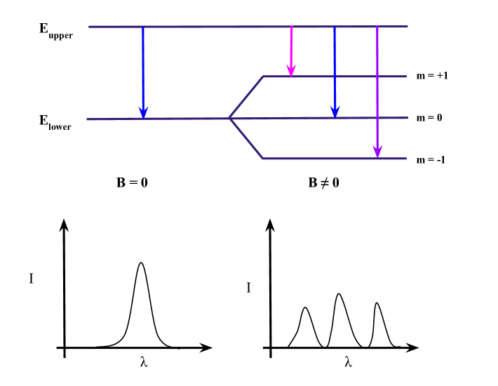
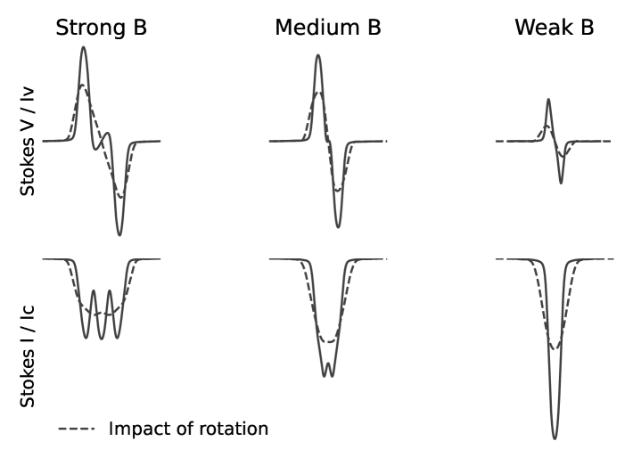
Figure 1: Left: Zeeman splitting of energy levels due to the presence of a magnetic field and the resulting intensity line profiles. On the left side is the case where $B=0$. The right side shows the case where $B\neq 0$. Here, we illustrate a so-called triplet (where only one of the level splits into 3 sub-levels), but the numbers of sub-levels depends on the specific quantum numbers associated with the energy levels. The resulting set of transitions is called a Zeeman pattern, and they can be quite varied (see e.g. del Toro Iniesta, 2003). Adapted from Figure 2 in Landstreet (2015). Right: Illustration of the impact of the dipolar field strength and stellar rotation on the Stokes I and V line profiles. Calculations made with the Unno-Rachkovsky solution (see del Toro Iniesta, 2003, for an overview) for a triplet with $\beta=i=45^{\circ}$ and $\phi=0$.

To measure the polarization from a star requires a spectropolarimeter, which is an instrument that can record both the intensity or Stokes I and one or more of the Stokes QUV parameters as a function of wavelength or spectrum. For stellar magnetism, the Stokes V spectrum is used to diagnose the presence of a field and multiple measurements throughout a star’s rotation can be used to study the magnetometry (the structure and geometry of the magnetic field).

A typical spectropolarimeter is placed into the incoming light beam of the telescope before the light is able to enter the spectrograph. The instrument contains a series of optical components, including a prism to split the beam into its two orthogonal polarization states so that the Stokes I spectrum and another Stokes parameter spectrum can be recorded simultaneously. The instrument also includes both half and quarter wave plates that are able to rotate, so that all three Stokes polarization parameters can be recorded without having to replace any optical components. In order to obtain a circular polarization or Stokes V spectrum, 4 individual observations must be made with the quarter and half wave plates at different angles that when combined they correspond to the mathematical representation for Stokes V. Data from four exposures are also combined in two other ways to obtain what are referred to as the Null spectra, as they do not combine to show any polarization, but instead allow the user to see if there are any optical residual signatures from the telescope or optical components within the instrument masking itself as real polarization signatures.

[]Examples of instruments used to study stellar magnetism

• FORS2 (R $\sim$ 2000) spectropolarimeter: optical low-resolution instrument installed on one of the 8-m Unit Telescopes (UT1) of the European Southern Observatory (ESO)’s Very Large Telescope (VLT) at the Paranal Observatory in Chile.

• ESPaDOnS (R = 65,000) spectropolarimeter: optical high-resolution instrument used on the 3-m Canada-France-Hawaii Telescope at the Mauna Kea Observatory in the USA. This is a twin of the Narval instrument at the 2.2-m Bernard Lyot Telescope at the Pic du Midi Observatory in France.

• HARPSpol (R = 105,000) spectropolarimeter: optical high-resolution instrument used on the 3.6-m ESO telescope at the La Silla Observatory in Chile.

• SPIRou (R = 75,000) spectropolarimeter: near-infrared high-resolution instrument used on the 3-m Canada-France-Hawaii Telescope at the Mauna Kea Observatory in the USA.

4 Measuring magnetic fields from spectropolarimetric data

To study magnetism in stars, we employ two types of techniques. High-resolution spectra provide detailed information of the stellar photospheric structure, revealing any small-scale variability. If a star is slowly rotating and has a strong magnetic field, the Zeeman splitting may be measured in individual lines, giving an estimation of the surface-averaged magnetic field strength. However, the typical spectral separation will only be about 1-2 km s${}^{-1}$ per kilogauss in the optical. So, unless the field is quite strong, the splitting will be less than the typical Doppler broadening of $\sim$ 5-10 km s${}^{-1}$. We may also use another additional type of observation called spectropolarimetry, which records spectroscopy and polarimetry simultaneously. Polarimetry provides a characterization of the magnetic structure of the star, including field strength, configuration, and geometry. Together, these two observed techniques produce a comprehensive data set to analyze and model the physical parameters of the star. Historically spectropolarimetry has been conducted using optical light, but infrared detectors are being used to study new types of objects, such as with SPIRou.

Spectropolarimetry can be used in two different methods, depending on the resolution of the instrument. For low-resolution optical spectropolarimeters, such as the FORS2 instrument on the VLT (and its predecessor FORS1), surface-averaged longitudinal magnetic field measurements, $B_{z}$, are obtained using the relationship

$$\frac{V}{I}=-g_{\mathrm{eff}}C_{Z}\lambda^{2}\frac{1}{I}\frac{dI}{d\lambda}\langle B_{z}\rangle,$$

where $B_{z}$ is the surface-averaged longitudinal magnetic field, $g_{\mathrm{eff}}$ is the effective Landé factor, $\lambda$ is the average wavelength, and $C_{Z}=\frac{e}{4\pi m_{e}c^{2}}$, where $m_{e}$ is the mass of an electron, and $e$ is the charge of an electron (for a basic review of this technique see, e.g., Bagnulo et al., 2015).

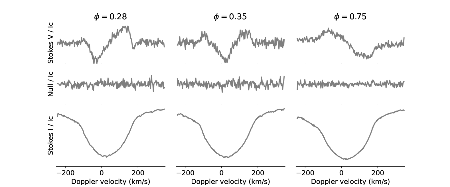
Figure 2: LSD Stokes I (bottom), null N (middle), and Stokes V (top) profiles for three different rotational phases of the proto-typical, He-strong Bp star $\sigma$ Ori E. For visualization purposes, the null and Stokes V have been shifted upwards from 0.0. The profile at rotational phase 0.35 shows an example of a case where the longitudinal field is close to zero, but the Stokes V signature is sill visible because of rotational broadening. The change or flip in polarity is viewed by comparing the Stokes V profile shapes at phase 0.28 to phase 0.75. The LSD profiles used in this figure are from Oksala et al. (2012).

For higher resolution optical or infrared spectropolarimeters, such as ESPaDOnS or SPIRou on CFHT, we can use the Stokes V data in individual lines to directly measure the surface-averaged longitudinal magnetic field strength ($B_{\ell}$, equivalent to $B_{z}$), if the field strength is large enough. However, a multi-line technique is often used to identify smaller field strengths and increase the signal-to-noise ratio (SNR), called Least Squares Deconvolution (LSD, Donati et al., 1997), which uses a list of spectral lines to make an effective average of the information contained in all of the lines simultaneously to produce an average Stokes I, null and Stokes V profile (see Fig. 2). This method assumes that the included lines have relatively similar shapes with amplitudes dictated by the characteristics of the individual lines (depth, magnetic sensitivity, etc) – therefore hydrogen lines are typically avoided.

Either using the individual signatures in lines or the LSD average profiles, $B_{\ell}$ can be derived from the Stokes V profile by computing the first moment of the Stokes V

$$B_{\ell}=-2.14\times 10^{11}\frac{\int vV(v)dv}{\lambda gc\int[I_{c}-I(v)]dv}~[\mathrm{G}],$$

where $g$ is the Landé factor (magnetic sensitivity) of the line or the average Landé factor if using the LSD line profile, $\lambda$ is the central wavelength (in nanometers) or the LSD average wavelength, and $c$, the speed of light, should have units of km s${}^{-1}$ (Donati et al., 1997; 2000MNRAS.313..851W). The integral is over velocity space, where the center of the line profile corresponds to $v=0$. The range of integration should typically be set so that it covers the entire spectral line. The value obtained for the longitudinal magnetic field often shows a variability related to rotation modulation of our view of the magnetic field geometry. To use this variability to estimate the dipolar field strength and the overall geometry of the system, i.e. the incidence angle, $i$, and the obliquity angle, $\beta$, we can employ the Preston Method, which is described in the boxed section below.

A statistical test called the False Alarm Probability (FAP) provides an objective test as to whether a magnetic field is detected for a star. The FAP is computed using the $\chi^{2}$ probability function associated with how much the Stokes V (and N) signal deviated from zero (see Donati et al., 1992, for more specific details). A signal is definitely detected (DD) in either V or N when the associated probability is larger than 99.999% or when the FAP is smaller than $10^{-5}$. A marginal detection (MD) corresponds to a FAP that is between $10^{-5}$ and $10^{-3}$. A FAP below $10^{-3}$ is considered a non-detection (ND; Donati et al., 1997).

[Bfield:Preston]The Preston method (1950MNRAS.110..395S; Preston, 1967)

The change in $B_{\ell}$ as the star rotates can be predicted under some simplifying assumptions:

1. The magnetic field is a dipole centered with the center of the star.

   • The magnetic field can be tilted by an angle $\beta$ with respect to the axis of rotation (the obliquity angle).

   • The axis of rotation can be tilted by an angle $i$ with respect to our line-of-sight to the star (the inclination angle)

2. The temperature structure in the photosphere of the star is such that we can assume that the source function of the radiation is linear with optical depth, which results in a so-called linear Limb-Darkening.

In this case, the relation between $B_{\ell}$ and the strength of the dipolar field $B_{p}$ is:

$$B_{\ell}=\frac{B_{p}}{20}\frac{15+u}{3-u}(\cos\beta\cos i+\sin\beta\sin i\cos\phi),$$

where $\phi$ is the rotational phase with $\phi=0$ corresponding to when a magnetic pole is the closest to our line-of-sight, and $u$ is the limb-darkening coefficient defined as $u=1-I_{\mathrm{limb}}/I_{\mathrm{center}}$ when $I$ is the intensity of the light at the center and limb of the stellar disk.

If we define a quantity $r$ as being the ratio of the minimum value to the maximum value of $B_{\ell}$ ($r=B_{\ell,\mathrm{min}}/B_{\ell,\mathrm{max}})$ and noting that these values of $B_{\ell}$ will occur when $\phi$ is $0$ and $\pi$, respectively, we can obtain a constraint between $i$ and $\beta$ that is independent of the polar strength or the limb-darkening coefficient:

$$\tan\beta=\left(\frac{1-r}{1+r}\right)\frac{1}{\tan i}$$

From a measured variation of $B_{\ell}$ (datapoints in figure below), we can employ e.g. sinusoidal fits (curves in left panel) to determine $B_{\ell,\mathrm{max}}$ and $B_{\ell,\mathrm{min}}$ (dashed lines), compute $r$, and obtained the constraints showed by the curves in the right panel. If one has a separate measurement of the inclination angle (for example from the combination of the rotation period, the rotational line broadening, and the star’s radius), the obliquity angle can then be constrained.

While there are many computational programs and tools to analyze spectropolarimetric observations of stars using various versions of Fortran, IDL, IRAF, etc., there has been a recent effort to create a centralized suite for analysis entirely in python. SpecpolFlow (Folsom et al., in prep) is a pythonic workflow that is a single pipeline for the analysis of spectropolarimetric observations of astronomical sources. The SpecpolFlow package is available at github.com/folsomcp/specpolFlow. In addition to building all of the tools necessary to take data directly from the telescope through to a full analysis with LSD, the team has also built a number of tutorials to ensure the tools are accessible to even novice users of spectropolarimetry.

If the Stokes V profile is rotationally modulated and one is able to obtain a time-series of spectropolarimetry sufficiently covering the rotation of a magnetic star, the technique of Zeeman Doppler imaging (ZDI) can be used to recover information about the magnetic topology and more accurately determine the geometry of the system (inclination, obliquity). ZDI combines the Stokes QUV lines from spectropolarimetry and a technique that uses Doppler broadening to map inhomogeneous structures on stellar surfaces called Doppler imaging. It was first proposed to be applied for magnetic fields by Semel (1989) and first implemented by e.g., Brown et al. (1991), inverting the Zeeman signatures onto a vector magnetic field surface distribution. Since then many implementations of this basic premise have led to mapping of magnetic structures. Current methods break down the magnetic structure of the poloidal or toroidal components of the field using spherical harmonic expansion (e.g., Donati et al., 2006; 2015MNRAS.453.2163S). This method of ZDI works for all types of magnetic stars, and can even use the LSD Stokes V profiles as input.

3 The intriguing origin of magnetic fields in hot stars

1 The definition of fossil fields

The magnetic fields of solar-type and low-mass stars are generated contemporaneously by a dynamo mechanism. This dynamo operates in the large convection zones present in these stars’ outer envelopes. The structure of a star is set by the temperature structure that determines where convection or radiation is more efficient to move energy from the core to the surface. For stars on the main sequence with masses larger than a few times the mass of our sun, the transport of energy in their outer layers can be done through radiation and no significant convection is expected in their outer-layers (see Kippenhahn et al., 2012, for details).

It was therefore surprising that surface magnetic fields on a star other than our own Sun were first detected in an intermediate-mass star (78 Vir, Babcock, 1947). Now, it has been established that about 10% of stars with radiative envelopes (intermediate stars and massive stars on the main sequence) have surface magnetic fields. Given that these fields are not from a solar-type dynamo, they have been dubbed fossil fields. The term originated from initial ideas that these fields might be caused by the concentration of ISM field lines during star formation (e.g. Mestel, 1965). Nowadays, the term fossil refers to any magnetic field that is not contemporaneously generated by a dynamo — they are a leftover from a “thing” that occurred in the star’s past, may it be an evolution phase, an event like a binary merger, or a mechanism during star formation. This said, it is important to note that some publications use “fossil origin scenario” to only mean the scenarios in which the fields originate from star formation, and do not refer to a magnetic origin from e.g. a binary interaction (that occurred in the past but after the star was born) as “fossil” – therefore some caution is needed.

2 Possible channels of formation

ISM

Magnetism is quite ubiquitous in all stages of star formation, from molecular filament to protostars (see Pattle et al., 2023). It would therefore not be surprising to find fossil stellar magnetic fields at the surface of main sequence stars. If anything, it could be viewed as rather strange that only 10% of main sequence massive stars end out being magnetic. The basic idea of the ISM fossil field hypothesis is that the ISM magnetic field can be pulled in and enhanced during the gravitational collapse. Some of the magnetic flux will inevitably be lost during this process due to various dissipation mechanisms, and only stars formed in areas of large enough initial fields would end up being magnetic (e.g., Mestel 1999). Some studies have shown that a magnetic field might inhibit the fragmentation of star-forming clouds (e.g. Price and Bate, 2008). There might therefore be a link between magnetism and mass, and/or between magnetism and binarity.

Mergers

Another interesting proposed channel for magnetism could be through binary interaction, where the magnetic fields are a by-product of a mass transfer or a merger event. About 30% of massive stars are expected to interact in their lifetime, and about 10% of them are even expected to merge into a single object (de Mink et al., 2014). During such an event, shear should give rise to magnetic fields according to MHD simulations (Schneider et al., 2019). It is the general consensus that merger products should appear “rejuvenated” (that is, appear younger than they really are) and fast rotating. However, recent theoretical studies of mergers incorporating magnetic fields (Schneider et al., 2020) have shown that fast rotation might not always be the typical outcome.

Subsurface convection

Main sequence massive O and B stars do have convection zones in their cores. There is both theoretical and observational (through asteroseismology) evidence that magnetic fields are generated in these convection zones (Augustson et al., 2016; Featherstone et al., 2009; Lecoanet et al., 2022). It is however understood that i) these dynamo-generated, core magnetic fields cannot reach the surface (MacDonald and Mullan, 2004) and ii) even if they could, we would then expect all stars with convection cores to have some degree of surface magnetic fields that correlate with the core properties — core dynamos therefore cannot readily explain the fossil field phenomenon.

Although we usually say that massive stars on the main sequence lack convection zones in their envelopes, we actually mean substantial convection zones. Massive stars with radiative envelopes still host thin, inefficient convection zones that are caused by opacity peaks from the ionization of hydrogen, helium, or iron-peak elements. These convection zones might be able to operate a dynamo, however, the magnetic fields emerging from these studies are usually expected to be weak and small-scaled (see Jermyn et al., 2022, for more details).

3 Incidence of magnetism in un-evolved OBA stars

Magnetic A and late-B (from spectral class B5 and cooler) stars on the main sequence have been better studied than their more massive counterparts, for a few reasons.

1. They have more spectral lines from metals in their optical spectra, which means that the multi-line techniques (REF to earlier section) are more effective.

2. Their spectral lines are narrower than those of hotter stars (less thermal, Stark, and rotational broadening), which means that the Stokes V signal has a higher amplitude for the same magnetic field value and therefore requires a smaller signal-to-noise ratio to detect.

3. They are more numerous in our local environment because the Initial Mass Function (see the Chapter on the IMF in this Encyclopedia) favors less massive stars. This helps with building enough statistics to enable general conclusions about their properties.

All of these properties make up for the fact that A and late-B stars are intrinsically less luminous than O and early-B stars.

Another important aspect that has enabled better studies of magnetic A and late-B stars is that they are easier to find by indirect methods. The atmospheres of these stars are very stable, which means that the chemical settling of various elements can take place without being disturbed by turbulence, outflows, or convection (see the chapter on chemically peculiar stars in this Encyclopedia). Magnetic A and late-B stars develop a specific abundance peculiarity pattern that is designated ApBp. There is a two-way relationship between magnetism and the ApBp classification: all strongly magnetic A and late-B stars have ApBp chemical peculiarity, and all stars with the ApBp chemical peculiarity have been found to be magnetic (e.g. Aurière et al., 2007). This means that magnetic A and late-B stars can be identified through spectroscopy only.

Furthermore, the distribution of elements is often not uniform at the surface of ApBp stars. There are patches of high or low abundances of various elements that often correlate with the structure of the magnetic field. Different abundances change the local flux emerging from various parts of the visible stellar disk. If there is an asymmetry in these patches with respect to the rotation axis of the star, the combined flux coming from the visible stellar disk will change as the star rotates. This means that photometric variations can also be used to identify ApBp stars (see e.g. Labadie-Bartz et al., 2023).

For hotter O and early-B stars, there are no direct two-way relationships between magnetism and chemical peculiarly. Some stars do display:

• the Of?p star classification (1972AJ.....77..312W), which relates to the relative strength of Ciii $\lambda\lambda$4647–4652Å and the Niii $\lambda\lambda$4634–4642Å lines (all Of?p stars have been found to be magnetic, but not all magnetic O-type stars have this spectral peculiarity).

• helium abundance peculiarities and He-line variations (e.g. Bohlender et al., 1987),

• variable and peculiar emission from their circumstellar magnetospheres (see review by 2022hxga.book...46U, for details).

Periodicity is therefore a good way to identify O and early-B magnetic candidates, and some surveys have successfully exploited this to pre-select stars with good likelihood of being magnetic (e.g. Buysschaert et al., 2018b). However, to compute the incidence of magnetic fields without selection-biases, it is necessary to confirm the presence of a magnetic field with spectropolarimetry for O and early-B stars.

[Bfield:rotation]Interesting fact

The rotation period of sun-like stars is easily determined by photometric variations due to magnetic spots. For magnetic massive stars, the photometric and spectral variations similarly can provide a rotational period as well. This period can sometimes be ambiguous, because the spectral and photometric diagnostics are not sensitive to the polarity of the magnetic field, which can sometime result in ambiguities between different period aliases. However, the magnetic fields of massive stars usually have a simple topology, and the variation of the longitudinal magnetic field measurements, which is sensitive to the field polarity, can typically lift these ambiguities.

For the 90% of massive stars that do not have a magnetic field, however, there are no good methods to identify rotation periods with good certainty. The line broadening gives us the equatorial velocity $v_{\mathrm{eq}}$ multiplied by the sin of the inclination of the rotational axis with respect to our line of sight $i$ ($v_{\mathrm{eq}}\sin i$). Fast rotating stars can be readily identified by their large $v_{\mathrm{eq}}\sin i$, but slow rotators are more difficult to identify as a fast rotating star could masquerade as a slowly rotating star if it has a small inclination angle $i$. Magnetic massive stars with long rotational period are therefore the perfect laboratory to e.g. study various types of non-rotational broadening such as macro-turbulence (2013MNRAS.433.2497S).

Incidence of main sequence magnetic ApBp and pre-main sequence Herbig AeBe stars

The general incidence of magnetism in main sequence A and late-B stars is around 10%. Fig. 17 of 2019MNRAS.483.2300S shows the distribution of incidence as a function of mass that was obtained from a 100-pc volume limited survey of ApBp stars. In their lower mass bin (1.4 - 1.6 $M_{\odot}$), the incidence is basically zero and rises to 10% by $\sim 3M_{\odot}$. This means that the transition from ubiquitous solar-type dynamo magnetism to a 10% of fossil field is not direct – there is a gap in magnetism around spectral type early-F star (see also Fig. 1 of Seach et al., 2020).

The presence of magnetic fields in A and late-B stars does not seem to correlate with stellar characteristics other than the ApBp phenomenon, which is a surface effect. ApBp stars occupy the same regions of the HRD as normal A and late-B stars (see Fig. 14 in 2019MNRAS.483.2300S). However, the bulk of the ApBp star population seems to rotate slower than their non-magnetic counterparts (Abt and Morrell, 1995), which is usually understood to be a consequence of magnetic braking.

Interestingly, fossil magnetic fields with similar characteristics to that of ApBp stars are already present during the pre-main sequence phase for these intermediate-mass stars. In a spectropolarimetric survey of about 70 Herbig AeBe stars, Alecian et al. (2013b, a) found that  7% of them host magnetic fields, all stronger than 300G.

Incidence of main sequence magnetic O and early-B stars

Similarly, for main sequence O and early-B stars, all large-scale surveys agree that the general incidence is a bit lower than 10%. Unlike for ApBp stars, massive OB stars are not as numerous in our local space, therefore volume-limited surveys are impractical. Therefore, most large-scale surveys are instead magnitude-limited, and prone to numerous selection biases. To give a sense of numbers, the Magnetism in Massive Stars (MiMeS) survey (2016MNRAS.456....2W) has found 6 new magnetic stars in a sample of 97 O-type stars (Grunhut et al., 2017), and the B Field in OB Stars (BOB) survey (Morel et al., 2014) has found 4 new magnetic stars in their sample of 69 OB-type stars (Schöller et al., 2017).

Again, there is no evidence of correlation of the incidence of magnetic field with stellar parameters, other than a loose correspondence with surface effects such as helium abundance peculiarities, magnetospheric emission, and the Of?p phenomenon. Magnetic O and early-B stars seem to roughly occupy the same region of the HRD as their non-magnetic counterparts (e.g. see Fig 10 from Grunhut et al., 2017). The rotation rates of magnetic massive OB stars are quite diverse. On one hand, most of the dozen or so known magnetic O-type stars have been found to be slow rotators (see the list of periods in Table 1 of Petit et al., 2013). Some periods are extremely long (for example the O8f?p star HD 108 with a 55-yr rotational period, Shultz and Wade, 2017). On the other hand, for magnetic early-B stars, some periods are measured in years (e.g. the B0.5 star $\xi^{1}$ CMa with $P\sim 30$ yr, Erba et al., 2021), whereas some are less than a day and nearly at critical velocity (e.g. the B2 star HR 7355 with $P\simeq 0.5$ d, Oksala et al., 2010).

4 Distribution of magnetic field strengths and the magnetic desert on the main sequence

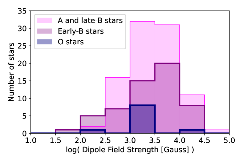
Figure 3: Distribution of magnetic dipolar strengths for A and late-B stars, early-B stars, and O stars. Note that the x-axis is in $\log_{10}$.
Adapted from Fig. 6 of 2019MNRAS.490..274S – small differences might be due to the specific columns used in the data sources, and the way the multi-pole results were tabulated (here we use the dipolar components only for simplicity): Aurière et al. (2007) Table 2 column $B_{d}$, 2019MNRAS.483.3127S Table 4 column $B_{d}$, Landstreet and Mathys (2000) Table 1 column $B_{d}$ (absolute value), 2019MNRAS.490..274S Table C2 column $B_{p}$, Petit et al. (2013) Table 1 column $B_{p}$ with the same modifications and additions as listed in 2019MNRAS.490..274S: 1000G for HD 108 from Shultz and Wade (2017), 140G for $\zeta$ Ori A from Blazère et al. (2015), and the addition of HD 54879 with the 1920G measurement from Järvinen et al. (2022).

Fig. 3 shows the distributions of magnetic field strengths (in kG) for a set of known O stars, early-B stars and late-B/A stars, from the sources listed in the caption. The distributions are very similar. 2019MNRAS.490..274S found that these distributions agree with a log-normal distribution with a mean of $10^{3.5}$ G and a standard deviation of $10^{0.6}$ G. Some of the stars with the largest magnetic fields known are in the range of tens of kG. Interestingly, if one was to shrink the most magnetic OB stars known to the size of a neutron star while conserving the magnetic flux (see Sect. 7), the surface field would be in the same order of magnitude as those of magnetars with $\sim 10^{15}$ G (Ferrario and Wickramasinghe, 2008).

On the lower end of the distribution, there are very few known magnetic stars with magnetic fields less than a few hundred Gauss. This could have been due to a magnetic detection threshold that prevents us from finding stars with small fields. However, Aurière et al. (2007) performed a survey of the Ap stars with the weakest polarization signals and found that they still have dipolar magnetic fields $>$300 G. Furthermore, surveys of non-Ap, A-type stars have not yielded any magnetic field detection with a precision below 300 G in most cases (e.g. Bagnulo et al., 2006). This lack of ApBp stars with $\sim 10$–100 G is called the Magnetic Desert.

This magnetic desert in ApBp stars was highlighted even more with the recent detection of so-called ultra-weak magnetic fields at the surface of the bright A-type stars Vega, Sirius A, $\beta$ UMa, $\theta$ Leo, and Alhena (Lignières et al., 2009; Petit et al., 2011; Blazère et al., 2016b, a). The shape of the circular polarization signal does not match what would be expected from the standard Zeeman effect theory for fossil fields. This said, if this signal is interpreted as a magnetic signal it would correspond to magnetic fields at the $\sim 1$ G level. These ultra-weak magnetic stars are still rare, because these observations are at the limit of the current technological capabilities of spectropolarimetry. This means that perhaps weak magnetism may be more ubiquitous than previously thought. On the other-hand, these Stokes V detections also underscore the presence of the magnetic desert – if $\sim$1 G level magnetic fields are detectable in A stars, magnetic fields of $\sim 10$–100 would have been detected by now, if they existed in main-sequence A-type stars.

For more massive O and early B-type stars, the detection capabilities are, in general, not as good as for A and late-B stars and highly depend on the characteristics and distance of the stars. For example, Petit et al. (2019) analyzed the dipolar field detection threshold for the O-type stars in the MiMeS Survey, and found that they ranged from 10 G to 1000 G, with a median of 85 G. From a Monte-Carlo analysis, if dipolar fields with strength of about 100G were ubiquitous in the MiMeS survey, they would have been found, which strengthens the idea that a magnetic desert might also exist for O-type stars.

As can be seen in Fig. 3, the distribution of magnetic B-type stars extend to slightly lower field strengths. Two B-type stars that are in the last third of the main sequence have been found with magnetic field dipolar strengths that could be lower than the strength threshold for ApBp stars ($\beta$ CMa $B_{d}>60$ and $\epsilon$ CMa $B_{d}>13$G Fossati et al., 2015). This could be indicative of a mass or age dependence on the Magnetic Desert’s threshold.

5 Topology of magnetic fields on the main sequence

Large surveys of the $B_{\ell}$ variation of the magnetic field of OBA stars have shown that they mainly have geometries that are close to dipolar (e.g. Bychkov et al., 2005). This said, when either precise $B_{\ell}$ curves are obtained or direct modeling of the Stokes V profiles is performed (e.g. ZDI), some additional medium-scale structures are nearly always found. The complexity of the magnetic field is often parametrized by either a multipole expansion (dipole$+$quadrupole$+$octople$+...$) or with spherical harmonics ($Y_{\ell}^{m}(\theta,\varphi)$). For example, Table 1 of Landstreet and Mathys (2000) shows that many Ap stars require significant quadrupolar and octopolar components to reproduce their $B_{\ell}$ variations with rotation. ZDI modeling of ApBp stars and O/early-B stars have also shown that some higher harmonics are often necessary. At the extreme, HD 37776 (B2IV) and $\tau$ Sco (B0.2V) are quite famous for their field structure for which the $\ell=3-4$ modes dominate (Kochukhov et al., 2011; Donati et al., 2006).

The tilt of the main dipolar component (the obliquity angle $\beta$ defined in Sect. 4) has been best studied for ApBp stars. Landstreet (1970) found that the magnetic axes are randomly distributed on the star, which means that larger $\beta$ will be favored with respect to the rotational axis. This is because the only one way to get $\beta=0$ is for the magnetic axis to be aligned with the rotational axis, but there are many more directions around a star that correspond to $\beta=90$.

Surprisingly, however, Landstreet and Mathys (2000) found that for Ap stars with long rotational periods ($>25$d) the magnetic axes tend to align more closely with the rotational axis (small values of $\beta$). For magnetic early-B stars, 2019MNRAS.490..274S found a distribution of $\beta$ angles compatible with a random orientation of the magnetic axis.

[Bfield:interesting]Did you know?

• HD 215441 (Babcock’s star) is the ApBp star with the strongest magnetic field (34 kG, Babcock, 1960).

• NGC 1624-2 is the O-type star with the largest magnetic field (20 kG, 2012MNRAS.425.1278W).

• HR 5907 is the magnetic early-B star with the fastest rotation period (0.5 d, Grunhut et al., 2012).

• HD 60431 is the ApBp star with the fastest rotation period (0.4 d, Mikulášek et al., 2022).

• HD 965 is the ApBp star with the longest period for which the magnetic field has been followed through a whole rotation (16 yr, Mathys et al., 2019).

• $\tau$ Sco and HD 37776 are two magnetic B-type stars with un-usually complex magnetic fields.

6 Magnetic Stars in binaries on the main sequence

Magnetic Ap stars are in wide binary systems as often as non-magnetic stars (Abt and Snowden, 1973). However, there is a complete lack of Ap in binaries with orbital periods shorter than 3 days (Carrier et al., 2002). There are also plenty of magnetic O and early-B stars in wide binary systems. However, the Binarity and Magnetic Interactions in various classes of Stars (BinaMIcS) Survey has only found a magnetic incidence of less than 2% in close binary systems with periods less than 20 days (Alecian et al., 2015). Overall, there are only about a dozen of known magnetic massive stars binaries with $P_{\mathrm{orb}}<20$ d (see Table 5 of Landstreet et al., 2017). There is only one known close binary system with two magnetic OBA stars: the B+B system $\epsilon$ Lup with an orbital period of 4 days (2015MNRAS.454L...1S).

Although rare, these binary systems are very interesting. For example, such binary stars are expected to be co-evolved. It is therefore a challenge for the ISM formation scenario to explain why one star is magnetic, and the other not. The lack of close binaries is certainly a point in favor of the merger field generation scenario. It is not clear, however, if this scenario can explain a system like $\epsilon$ Lup.

[Bfield:binary]Some noteworthy magnetic binary systems

• Plaskett’s star (HD 47129) is the only close massive binary that contains a magnetic O-type star (Grunhut et al., 2013, 2022). It is also the only fast-rotating magnetic O-type star.

• HD 45166 is a binary system containing a low-mass (2$M_{\odot}$) Wolf-Rayet (WR) star with a magnetic field of 43 kG in a wide orbit around a non-magnetic late-B star. There is good evidence that the WR star might be a merger product (Shenar et al., 2023). HD 148937 is another potential merger product (Frost et al., 2024).

• HD 66051 is the first eclipsing binary that contains an early-type star (Kochukhov et al., 2018).

7 Evolution of magnetic fields in massive stars

The magnetic field strength of a fossil field may change for a few reasons. If there are no other mechanisms to increase or decrease the strength of a fossil magnetic field, it will experience a slow decline called Ohmic decay. This decay has a characteristic time-scale that is given by

$$t_{Ohmic}=\frac{4\pi L^{2}\sigma}{c^{2}},$$

where $L$ is the scale size of the system, $\sigma$ is the electrical conductivity, and $c$ is the speed of light. If the magnetic field strength declines faster or slower than this time-scale, there may be other effects or stellar changes driving increases or decreases in the field strength. As an important example for evolving stars, if a star experiences an increase in radius, that change in radius should affect the surface magnetic field because of the concept of flux conservation. Because most massive stars are mainly ionized, plasma flows cannot cross magnetic field lines due to the Lorentz forces. Therefore, either the plasma has to flow along field lines, or the field lines have to get dragged by the flow, depending on the relative strength of the field and the flow. In the case of the interior of a star, the latter generally applies. As a star expends in radius, the field lines will find themselves further apart, and the density of field lines (which is the definition of magnetic field strength) will be lowered.

The magnetic flux over the surface of the star is generally approximated by $\phi\approx 4\pi R^{2}B_{surf}$ (and often, the factor of $4\pi$ is even ignored). Assuming an initial radius and surface magnetic field, for example the radius at the zero-age main sequence, the effect of a radius change on the surface magnetic field strength under flux conservation can be computed from

$$B_{surf}(t)=B_{surf}(t_{ZAMS})\left(\frac{R(t_{ZAMS})}{R(t)}\right)^{2}.$$

This relationship implies that as the star increases in radius, its surface magnetic field would be expected to decrease as the square of the radius. Additionally, the development of convective outer layers that may develop during post-main sequence evolution (e.g., Featherstone et al., 2009) could complicate the large-scale magnetic fields of OBA stars, creating the possibility of dynamo fields developing in those layers, either enhancing or diminishing any surface fields.

Magnetic evolution on the Main Sequence

Observationally, we find a change in field strength of OBA stars as a function of stellar age – this is expected, as the radius is expected to change by a factor of a few over the MS (Landstreet et al., 2008; 2019MNRAS.490..274S). An interesting question is whether the magnetic flux is observationally conserved on the MS. To answer this, we need to determine the expected change in radius from evolution models. Typically, the associated additional systematic uncertainties are such that the age determination needs to be rather precise to evaluate the evolution of the magnetic flux. The best age estimates come from stars that are members of clusters. This is especially true for ApBp stars, because the uncertain bolometric correction calibration for ApBp stars (due to their abundance peculiarities impacting their color, as discussed in detail in Landstreet et al., 2007) makes their position on the HRD more uncertain.

Landstreet et al. (2008) found that for ApBp cluster members with masses between 2$M_{\odot}$ and 5$M_{\odot}$, the observations are constant with a small decrease in magnetic flux over the MS lifetime. 2019MNRAS.490..274S found that the magnetic flux of field and cluster magnetic OB-type stars also seem to decrease on the main sequence by a factor of a few. Although they note that for the most massive stars, the evolution tracks used to determine stellar ages and main sequence lifetimes do not include the impact of magnetism on stellar structure and evolution, which might be significant for the most massive O-stars.

Another approach is to study the incidence of magnetic stars as a function of time. For example, Fossati et al. (2016) constructed a probability density distribution of fractional main-sequence age for all of the magnetic OB stars known at the time. They compared this distribution to that of a representative magnitude-limited survey of normal OB stars and the expected sensitivity from modern spectropolarimetric instruments. They found that the age distribution of the comparison sample was dominated by stars in the last quarter of their MS lifetime, whereas the distribution of magnetic stars peaked in the middle of the main sequence lifetime. This would indicate a lack of old magnetic MS stars. Unfortunately, the detection limits actually achieved by the MiMeS Survey — at least for O-type stars, while compatible with magnetic flux conservation, were not low enough to convincingly establish constraints on flux decay on the MS (Petit et al., 2019).

Magnetic evolution after the Main Sequence

As stars leave the main sequence, ceasing hydrogen fusion reactions in their core, they will typically experience physical changes to surface temperature, physical radius, and some may experience a change in structure, i.e., the development of a convective layer. In these more evolved stars, the large-scale stable magnetic fields seen in main sequence OBA stars will inevitably be affected by such changes. New modeling and theoretical studies have aimed to build in the possible effects that these fields may have on the interior structure and evolutionary path of OBA stars (see e.g., Maeder and Meynet, 2003; 2016A&A...585A.120S). Many studies and more recent work, for example the work of Keszthelyi et al. (2019) (and other papers in that series), have tried to build in the effects of the magnetic field in a physically realistic manner. For more information on this, we recommend the recent review article by Keszthelyi (2023). Understanding how the magnetic field affects the star as it evolves and vice versa remains a challenging area of research.

Efforts to understand the problem from the observational side have faced different challenges. One of the first confirmed magnetic fields in a star evolved from an OBA star was EK Eridani and the study of Aurière et al. (2008). The first O supergiant with a weak detected magnetic field was $\zeta$ Ori Aa, which was determined to be magnetic by Bouret et al. (2008), and confirmed by Blazère et al. (2015). Several surveys have investigated red giant and supergiants that have evolved from main sequence OBA stars (see e.g., Grunhut et al., 2010; Aurière et al., 2015), and found for these stars that dynamo fields did develop in convective zones, affecting the observation of any previous main sequence magnetism due to a fossil field on the stellar surface.

The discovery of two significantly evolved A supergiants, $\iota$ Car and HR 3890, with longitudinal magnetic field strengths of just a few G (Neiner et al., 2017), confirmed that study of evolved OBA stars would require significantly lower uncertainties due to small field strengths that were consistent with flux conservation. From this the Large Impact of magnetic Fields on the Evolution of hot stars (LIFE) project was started to systematically use high-precision spectropolarimetric observations to investigate the magnetism of OBA supergiants. The goal was to understand how stellar magnetism works in their transitional evolutionary phases. Martin et al. (2018) reported early results, which appear to be consistent with magnetic flux conservation, but the overall survey results are still in progress. This type of study faces challenges: (1) high-precision observations of many supergiants require significant observational time, and (2) the number of such realistically observable targets is smaller, making significant statistical conclusions, such as those done for main sequence populations, more difficult.

4 Conclusions

Stellar magnetism affects all types of stars throughout their lifetimes. It can greatly modify their internal and external properties and how their evolutionary path proceeds. For OBA type stars, we find a fossil magnetic field different from that found for the Sun, and only a $\sim$10% incidence rate. We have discussed some of the known properties of these types of stars and some of the ways we observe and study them.

But, stellar magnetism is just one aspect of the physical processes involved in stars, therefore we cannot always consider it as acting on its own. We have mentioned throughout this chapter some cases of this as magnetic fields affect the atmospheres of stars, creating chemically peculiar stars with inhomogenous surface abundances, and the interaction of the magnetic field with stellar winds to create magnetospheric structures. Another intersection that stars with magnetic fields may have is with stellar pulsation (see the Chapter on Asteroseismology in this Encyclopedia).

Several categories of OBA pulsating stars are also known to possess a fossil magnetic field. roAp stars have been long known to have strong dipolar magnetic fields and stellar pulsations (Kurtz, 1990). Both slowly pulsating B (SPB) stars (e.g., Neiner et al., 2003) and $\beta$ Cep (see e..g., Henrichs et al., 2013; Briquet et al., 2012) stars have measured magnetic fields that have been well studied also in pulsation observations (see e.g., Briquet et al., 2016). Most recently, the pulsating $\delta$ Scuti stars have been discovered to have magnetic fields (see e.g, Neiner and Lampens, 2015).

Studying the interiors of stars using asteroseismology is already a challenging task, but the presence of a strong fossil magnetic field can affect various aspects of the pulsational observations. For example, pulsational frequencies are split by the presence of the magnetic field. The properties of the resulting frequencies depends on both the strength of the magnetic field and the magnetic geometry (see e.g., Shibahashi and Aerts, 2000). The magnetic field can also affect the period spacing for gravity-mode pulsations, which can then be used to estimate the strength of the internal magnetic field (see e.g., Prat et al., 2020). Recent work by Li et al. (2022) has used this effect to infer the strength of the internal magnetic fields in the cores of a sample of red giants.

To properly study the dual effects of pulsation and magnetic fields in a star requires a new type of technique. Magneto-asteroseismology evaluates the magnetic effects and the pulsational effects simultaneously to accurately determine both properties. This technique is crucial to understand the impact of magnetism on the internal dynamics and evolution of these stars. Thus far, only one star, the SPB HD 43317 has been analyzed combining both magnetic and pulsational effects (Buysschaert et al., 2018a), and by adding in MHD simulations, Lecoanet et al. (2022) were able to make the first estimate of the magnetic field strength inside a star on the main sequence. Stellar asteroseismology and magneto-asteroseismology are a relatively new field and technique that will grow as high-precision, long-term photometry continues to become available.

Magneto-Asteroseisomology is just one example of studying two effects together to gain a more complete picture of the effects of physical processes. We can imagine that the future of studying magnetic fields in stars will continue to connect with other physical mechanisms as we learn more about how they are intertwined.

[Acknowledgments]

VP is supported by the National Science Foundation (NSF) under Grant AST-2108455. MEO is supported by the National Science Foundation (NSF) under Grant AST-2107871. We thank the editor Fabian Schneider for expert feedback and insightful suggestions.

see also Donati and Landstreet (2009), Linsky and Schöller (2015) 102

Abt HA and Morrell NI (1995), Jul. The Relation between Rotational Velocities and Spectral Peculiarities among A-Type Stars. ApJS 99: 135. 10.1086/192182.

Abt HA and Snowden MS (1973), Feb. The Binary Frequency for AP Stars. ApJS 25: 137. 10.1086/190265.

Alecian E, Wade GA, Catala C, Grunhut JH, Landstreet JD, Bagnulo S, Böhm T, Folsom CP, Marsden S and Waite I (2013a), Feb. A high-resolution spectropolarimetric survey of Herbig Ae/Be stars - I. Observations and measurements. MNRAS 429: 1001–1026.

Alecian E, Wade GA, Catala C, Grunhut JH, Landstreet JD, Böhm T, Folsom CP and Marsden S (2013b), Feb. A high-resolution spectropolarimetric survey of Herbig Ae/Be stars - II. Rotation. MNRAS 429: 1027–1038.

Alecian E, Neiner C, Wade GA, Mathis S, Bohlender D, Cébron D, Folsom C, Grunhut J, Le Bouquin JB, Petit V, Sana H, Tkachenko A and ud-Doula A (2015), Jan., The BinaMIcS project: understanding the origin of magnetic fields in massive stars through close binary systems, Meynet G, Georgy C, Groh J and Stee P, (Eds.), New Windows on Massive Stars, IAU Symposium, 307, 330–335, 1409.1094.

Augustson KC, Brun AS and Toomre J (2016), Mar. The Magnetic Furnace: Intense Core Dynamos in B-stars. ArXiv e-prints 1603.03659.

Aurière M, Wade GA, Silvester J, Lignières F, Bagnulo S, Bale K, Dintrans B, Donati JF, Folsom CP, Gruberbauer M, Bon Hoa AH, Jeffers S, Johnson N, Landstreet JD, Lèbre A, Lueftinger T, Marsden S, Mouillet D, Naseri S, Paletou F, Petit P, Power J, Rincon F, Strasser S and Toqué N (2007), Dec. Weak magnetic fields in Ap/Bp stars. Evidence for a dipole field lower limit and a tentative interpretation of the magnetic dichotomy. A&A 475: 1053–1065.

Aurière M, Konstantinova-Antova R, Petit P, Charbonnel C, Dintrans B, Lignières F, Roudier T, Alecian E, Donati JF, Landstreet JD and Wade GA (2008), Nov. EK Eridani: the tip of the iceberg of giants which have evolved from magnetic Ap stars. A&A 491 (2): 499–505. 10.1051/0004-6361:200810502. 0810.2228.

Aurière M, Konstantinova-Antova R, Charbonnel C, Wade GA, Tsvetkova S, Petit P, Dintrans B, Drake NA, Decressin T, Lagarde N, Donati JF, Roudier T, Lignières F, Schröder KP, Landstreet JD, Lèbre A, Weiss WW and Zahn JP (2015), Feb. The magnetic fields at the surface of active single G-K giants. A&A 574, A90. 10.1051/0004-6361/201424579. 1411.6230.

Babcock HW (1947), Jan. Zeeman Effect in Stellar Spectra. ApJ 105: 105.

Babcock HW (1960), Nov. The 34-KILOGAUSS Magnetic Field of HD 215441. ApJ 132: 521.

Bagnulo S, Landstreet JD, Mason E, Andretta V, Silaj J and Wade GA (2006), May. Searching for links between magnetic fields and stellar evolution. I. A survey of magnetic fields in open cluster A- and B-type stars with FORS1. A&A 450: 777–791.

Bagnulo S, Fossati L, Landstreet JD and Izzo C (2015), Nov. The FORS1 catalogue of stellar magnetic field measurements. A&A 583, A115. 10.1051/0004-6361/201526497. 1508.03839.

Blazère A, Neiner C, Tkachenko A, Bouret JC and Rivinius T (2015), Oct. The magnetic field of $\zeta$ Orionis A. A&A 582, A110. 10.1051/0004-6361/201526855. %****␣MagneticStars.bbl␣Line␣175␣****1509.02773.

Blazère A, Neiner C and Petit P (2016a), Jun. Discovery of a very weak magnetic field on the Am star Alhena. MNRAS 459 (1): L81–L84. 10.1093/mnrasl/slw050. 1603.06486.

Blazère A, Petit P, Lignières F, Aurière M, Ballot J, Böhm T, Folsom CP, Gaurat M, Jouve L, Lopez Ariste A, Neiner C and Wade GA (2016b), Feb. Detection of ultra-weak magnetic fields in Am stars: $\beta$ Ursae Majoris and $\theta$ Leonis. A&A 586: A97.

Bohlender DA, Landstreet JD, Brown DN and Thompson IB (1987), Dec. Magnetic field measurements of helium-strong stars. ApJ 323: 325–337.

Bouret JC, Donati JF, Martins F, Escolano C, Marcolino W, Lanz T and Howarth ID (2008), Sep. The weak magnetic field of the O9.7 supergiant $\zeta$OrionisA. MNRAS 389 (1): 75–85. 10.1111/j.1365-2966.2008.13575.x. 0806.2162.

Briquet M, Neiner C, Aerts C, Morel T, Mathis S, Reese DR, Lehmann H, Costero R, Echevarria J, Handler G, Kambe E, Hirata R, Masuda S, Wright D, Yang S, Pintado O, Mkrtichian D, Lee BC, Han I, Bruch A, De Cat P, Uytterhoeven K, Lefever K, Vanautgaerden J, de Batz B, Frémat Y, Henrichs H, Geers VC, Martayan C, Hubert AM, Thizy O and Tijani A (2012), Nov. Multisite spectroscopic seismic study of the $\beta$ Cep star V2052 Ophiuchi: inhibition of mixing by its magnetic field. MNRAS 427 (1): 483–493. 10.1111/j.1365-2966.2012.21933.x. 1208.4250.

Briquet M, Neiner C, Petit P, Leroy B and de Batz B (2016), Mar. Weak magnetic field, solid-envelope rotation, and wave-induced N-enrichment in the SPB star $\zeta$ Cassiopeiae. A&A 587, A126. 10.1051/0004-6361/201527751. 1601.04517.

Brown SF, Donati JF, Rees DE and Semel M (1991), Oct. Zeeman-Doppler imaging of solar-type and AP stars. IV. Maximum entropy reconstruction of 2D magnetic topologies. A&A 250: 463.

Buysschaert B, Aerts C, Bowman DM, Johnston C, Van Reeth T, Pedersen MG, Mathis S and Neiner C (2018a), Aug. Forward seismic modeling of the pulsating magnetic B-type star HD 43317. A&A 616, A148. 10.1051/0004-6361/201832642. 1805.00802.

Buysschaert B, Neiner C, Martin AJ, Aerts C, Bowman DM, Oksala ME and Van Reeth T (2018b), Aug. Detection of magnetic fields in chemically peculiar stars observed with the K2 space mission. MNRAS 478 (2): 2777–2793. 10.1093/mnras/sty1190. 1805.00781.

Bychkov VD, Bychkova LV and Madej J (2005), Feb. A catalog of stellar magnetic rotational phase curves. A&A 430: 1143–1154.

Carrier F, North P, Udry S and Babel J (2002), Oct. Multiplicity among chemically peculiar stars. II. Cool magnetic Ap stars. A&A 394: 151–169. 10.1051/0004-6361:20021122. astro-ph/0208082.

de Mink SE, Sana H, Langer N, Izzard RG and Schneider FRN (2014), Feb. The Incidence of Stellar Mergers and Mass Gainers among Massive Stars. ApJ 782 (1), 7. 10.1088/0004-637X/782/1/7. 1312.3650.

del Toro Iniesta JC (2003), Apr. Introduction to Spectropolarimetry, Cambridge University Press, Cambridge, UK.

Donati JF and Landstreet JD (2009), Sep. Magnetic Fields of Nondegenerate Stars. ARA&A 47 (1): 333–370. 10.1146/annurev-astro-082708-101833. 0904.1938.

Donati JF, Semel M and Rees DE (1992), Nov. Circularly polarized spectroscopic observations of RS CVn systems. A&A 265: 669–681.

Donati JF, Semel M, Carter BD, Rees DE and Collier Cameron A (1997), Nov. Spectropolarimetric observations of active stars. MNRAS 291 (4): 658–682. 10.1093/mnras/291.4.658.

Donati JF, Howarth ID, Jardine MM, Petit P, Catala C, Landstreet JD, Bouret JC, Alecian E, Barnes JR, Forveille T, Paletou F and Manset N (2006), Aug. The surprising magnetic topology of $\tau$ Sco: fossil remnant or dynamo output? MNRAS 370 (2): 629–644. 10.1111/j.1365-2966.2006.10558.x. astro-ph/0606156.

Erba C, Shultz ME, Petit V, Fullerton AW, Henrichs HF, Kochukhov O, Rivinius T and Wade GA (2021), Sep. Confirmation of $\xi$${}^{1}$ CMa’s ultra-slow rotation: magnetic polarity reversal and a dramatic change in magnetospheric UV emission lines. MNRAS 506 (2): 2296–2308. 10.1093/mnras/stab1454. 2105.08192.

Featherstone NA, Browning MK, Brun AS and Toomre J (2009), Nov. Effects of Fossil Magnetic Fields on Convective Core Dynamos in A-type Stars. ApJ 705: 1000–1018.

Ferrario L and Wickramasinghe D (2008), Sep. Origin and evolution of magnetars. MNRAS 389: L66–L70.

Fossati L, Castro N, Morel T, Langer N, Briquet M, Carroll TA, Hubrig S, Nieva MF, Oskinova LM, Przybilla N, Schneider FRN, Schöller M, Simón-Díaz S, Ilyin I, de Koter A, Reisenegger A and Sana H (2015), Feb. B fields in OB stars (BOB): on the detection of weak magnetic fields in the two early B-type stars $\beta$ CMa and $\epsilon$ CMa. Possible lack of a magnetic desert in massive stars. A&A 574, A20. 10.1051/0004-6361/201424986. %****␣MagneticStars.bbl␣Line␣425␣****1411.6490.

Fossati L, Schneider FRN, Castro N, Langer N, Simón-Díaz S, Müller A, de Koter A, Morel T, Petit V, Sana H and Wade GA (2016), Aug. Evidence of magnetic field decay in massive main-sequence stars. A&A 592, A84. 10.1051/0004-6361/201628259. 1606.07599.

Frost AJ, Sana H, Mahy L, Wade G, Barron J, Le Bouquin JB, Mérand A, Schneider FRN, Shenar T, Barbá RH, Bowman DM, Fabry M, Farhang A, Marchant P, Morrell NI and Smoker JV (2024), Apr. A magnetic massive star has experienced a stellar merger. Science 384 (6692): 214–217. 10.1126/science.adg7700. 2404.10167.

Grunhut JH, Wade GA, Hanes DA and Alecian E (2010), Nov. Systematic detection of magnetic fields in massive, late-type supergiants. MNRAS 408 (4): 2290–2297. 10.1111/j.1365-2966.2010.17275.x. 1006.5891.

Grunhut JH, Rivinius T, Wade GA, Townsend RHD, Marcolino WLF, Bohlender DA, Szeifert T, Petit V, Matthews JM, Rowe JF, Moffat AFJ, Kallinger T, Kuschnig R, Guenther DB, Rucinski SM, Sasselov D and Weiss WW (2012), Jan. HR 5907: Discovery of the most rapidly rotating magnetic early B-type star by the MiMeS Collaboration. MNRAS 419: 1610–1627.

Grunhut JH, Wade GA, Leutenegger M, Petit V, Rauw G, Neiner C, Martins F, Cohen DH, Gagné M, Ignace R, Mathis S, de Mink SE, Moffat AFJ, Owocki S, Shultz M, Sundqvist J and MiMeS Collaboration (2013), Jan. Discovery of a magnetic field in the rapidly rotating O-type secondary of the colliding-wind binary HD 47129 (Plaskett’s star). MNRAS 428: 1686–1695.

Grunhut JH, Wade GA, Neiner C, Oksala ME, Petit V, Alecian E, Bohlender DA, Bouret JC, Henrichs HF, Hussain GAJ, Kochukhov O and MiMeS Collaboration (2017), Feb. The MiMeS survey of Magnetism in Massive Stars: magnetic analysis of the O-type stars. MNRAS 465: 2432–2470. 10.1093/mnras/stw2743. 1610.07895.

Grunhut JH, Wade GA, Folsom CP, Neiner C, Kochukhov O, Alecian E, Shultz M, Petit V, MiMeS Collaboration and BinaMIcS Collaboration (2022), May. The magnetic field and magnetosphere of Plaskett’s star: a fundamental shift in our understanding of the system. MNRAS 512 (2): 1944–1966. 10.1093/mnras/stab3320. 2111.06251.

Henrichs HF, de Jong JA, Verdugo E, Schnerr RS, Neiner C, Donati JF, Catala C, Shorlin SLS, Wade GA, Veen PM, Nichols JS, Damen EMF, Talavera A, Hill GM, Kaper L, Tijani AM, Geers VC, Wiersema K, Plaggenborg B and Rygl KLJ (2013), Jul. Discovery of the magnetic field in the pulsating B star $\beta$ Cephei. A&A 555, A46. 10.1051/0004-6361/201321584. 1305.2601.

Järvinen SP, Hubrig S, Schöller M, Cikota A, Ilyin I, Hummel CA and Küker M (2022), Mar. Detection of anomalous element distribution in the extremely slowly rotating magnetic O9.7 V star HD 54879. MNRAS 510 (3): 4405–4419. 10.1093/mnras/stab3720. 2112.14362.

Jermyn AS, Anders EH, Lecoanet D and Cantiello M (2022), Sep. An Atlas of Convection in Main-sequence Stars. ApJS 262 (1), 19. 10.3847/1538-4365/ac7cee. 2206.00011.

Keszthelyi Z (2023), Mar. Magnetism in High-Mass Stars. Galaxies 11 (2): 40. 10.3390/galaxies11020040. 2303.02878.

Keszthelyi Z, Meynet G, Georgy C, Wade GA, Petit V and David-Uraz A (2019), Jun. The effects of surface fossil magnetic fields on massive star evolution: I. Magnetic field evolution, mass-loss quenching, and magnetic braking. MNRAS 485 (4): 5843–5860. 10.1093/mnras/stz772. 1902.09333.

Kippenhahn R, Weigert A and Weiss A (2012). Stellar Structure and Evolution. 10.1007/978-3-642-30304-3.

Kochukhov O, Lundin A, Romanyuk I and Kudryavtsev D (2011), Jan. The Extraordinary Complex Magnetic Field of the Helium-strong Star HD 37776. ApJ 726: 24.

Kochukhov O, Johnston C, Alecian E, Wade GA and BinaMIcS Collaboration (2018), Aug. HD 66051: the first eclipsing binary hosting an early-type magnetic star. MNRAS 478 (2): 1749–1762. 10.1093/mnras/sty1118. 1804.10537.

Kurtz DW (1990), Jan. Rapidly oscillating AP stars. ARA&A 28: 607–655. 10.1146/annurev.aa.28.090190.003135.

Labadie-Bartz J, Hümmerich S, Bernhard K, Paunzen E and Shultz ME (2023), Aug. Photometric variability of the LAMOST sample of magnetic chemically peculiar stars as seen by TESS. A&A 676, A55. 10.1051/0004-6361/202346657. 2306.12861.

Landstreet JD (1970), Mar. The Orientation of Magnetic Axes in the Magnetic Variables. ApJ 159: 1001. 10.1086/150377.

Landstreet JD (2015), Jan., Basics of spectropolarimetry, Meynet G, Georgy C, Groh J and Stee P, (Eds.), New Windows on Massive Stars, IAU Symposium, 307, 311–320.

Landstreet JD and Mathys G (2000), Jul. Magnetic models of slowly rotating magnetic Ap stars: aligned magnetic and rotation axes. A&A 359: 213–226.

Landstreet JD, Bagnulo S, Andretta V, Fossati L, Mason E, Silaj J and Wade GA (2007), Aug. Searching for links between magnetic fields and stellar evolution: II. The evolution of magnetic fields as revealed by observations of Ap stars in open clusters and associations. A&A 470: 685–698.

Landstreet JD, Silaj J, Andretta V, Bagnulo S, Berdyugina SV, Donati J, Fossati L, Petit P, Silvester J and Wade GA (2008), Apr. Searching for links between magnetic fields and stellar evolution. III. Measurement of magnetic fields in open cluster Ap stars with ESPaDOnS. A&A 481: 465–480.

Landstreet JD, Kochukhov O, Alecian E, Bailey JD, Mathis S, Neiner C, Wade GA and BINaMIcS Collaboration (2017), May. BD-19 5044L: discovery of a short-period SB2 system with a magnetic Bp primary in the open cluster IC 4725. A&A 601, A129. 10.1051/0004-6361/201630233. 1701.06945.

Lecoanet D, Bowman DM and Van Reeth T (2022), May. Asteroseismic inference of the near-core magnetic field strength in the main-sequence B star HD 43317. MNRAS 512 (1): L16–L20. 10.1093/mnrasl/slac013. 2202.03440.

Li G, Deheuvels S, Ballot J and Lignières F (2022), Oct. Magnetic fields of 30 to 100 kG in the cores of red giant stars. Nature 610 (7930): 43–46. 10.1038/s41586-022-05176-0. 2208.09487.

Lignières F, Petit P, Böhm T and Aurière M (2009), Jun. First evidence of a magnetic field on ¡ASTROBJ¿Vega¡/ASTROBJ¿. Towards a new class of magnetic A-type stars. A&A 500 (3): L41–L44.

Linsky JL and Schöller M (2015), Oct. Observations of Strong Magnetic Fields in Nondegenerate Stars. Space Sci. Rev. 191 (1-4): 27–76. 10.1007/s11214-015-0143-1.

MacDonald J and Mullan DJ (2004), Feb. Magnetic fields in massive stars: dynamics and origin. MNRAS 348 (2): 702–716. 10.1111/j.1365-2966.2004.07394.x.

Maeder A and Meynet G (2003), Dec. Stellar evolution with rotation and magnetic fields. I. The relative importance of rotational and magnetic effects. A&A 411: 543–552. 10.1051/0004-6361:20031491. astro-ph/0309672.

Martin AJ, Neiner C, Oksala ME, Wade GA, Keszthelyi Z, Fossati L, Marcolino W, Mathis S and Georgy C (2018), Apr. First results from the LIFE project: discovery of two magnetic hot evolved stars. MNRAS 475 (2): 1521–1536. 10.1093/mnras/stx3264. 1712.07403.

Mathys G, Romanyuk II, Hubrig S, Kudryavtsev DO, Schöller M, Semenko EA and Yakunin IA (2019), Sep. HD 965: An extremely peculiar A star with an extremely long rotation period. A&A 629, A39. 10.1051/0004-6361/201936092. 1907.10675.

Mestel L (1965), ”Fossil” magnetic fields, T. Gold, (Ed.), Stellar and Solar Magnetic Fields, IAU Symposium, 22, pp. 420.

Mikulášek Z, Semenko E, Paunzen E, Hümmerich S, North PL, Bernhard K, Krtička J and Janík J (2022), Dec. HD 60431, the CP2 star with the shortest rotational period. Physical parameters and period analysis. A&A 668, A159. 10.1051/0004-6361/202243622. 2209.12207.

Morel T, Castro N, Fossati L, Hubrig S, Langer N, Przybilla N, Schöller M, Carroll T, Ilyin I, Irrgang A, Oskinova L, Schneider FRN, Díaz SS, Briquet M, González JF, Kharchenko N, Nieva MF, Scholz RD, de Koter A, Hamann WR, Herrero A, Maíz Apellániz J, Sana H, Arlt R, Barbá R, Dufton P, Kholtygin A, Mathys G, Piskunov A, Reisenegger A, Spruit H and Yoon SC (2014), Sep. The B Fields in OB Stars (BOB) Survey. The Messenger 157: 27–31.

Neiner C and Lampens P (2015), Nov. First discovery of a magnetic field in a main-sequence $\delta$ Scuti star: the Kepler star HD 188774. MNRAS 454 (1): L86–L90. 10.1093/mnrasl/slv130. 1508.07273.

Neiner C, Geers VC, Henrichs HF, Floquet M, Frémat Y, Hubert AM, Preuss O and Wiersema K (2003), Aug. Discovery of a magnetic field in the Slowly Pulsating B star ¡ASTROBJ¿zeta Cassiopeiae¡/ASTROBJ¿. A&A 406: 1019–1031. 10.1051/0004-6361:20030742.

Neiner C, Oksala ME, Georgy C, Przybilla N, Mathis S, Wade G, Kondrak M, Fossati L, Blazère A, Buysschaert B and Grunhut J (2017), Oct. Discovery of magnetic A supergiants: the descendants of magnetic main-sequence B stars. MNRAS 471 (2): 1926–1935. 10.1093/mnras/stx1549. 1707.00560.

Oksala ME, Wade GA, Marcolino WLF, Grunhut J, Bohlender D, Manset N and Townsend RHD (2010), Jun. Discovery of a strong magnetic field in the rapidly rotating B2Vn star HR 7355. MNRAS 405: L51–L55.

Oksala ME, Wade GA, Townsend RHD, Owocki SP, Kochukhov O, Neiner C, Alecian E and Grunhut J (2012), Jan. Revisiting the Rigidly Rotating Magnetosphere model for $\sigma$ Ori E - I. Observations and data analysis. MNRAS 419: 959–970.

Pattle K, Fissel L, Tahani M, Liu T and Ntormousi E (2023), Jul., Magnetic Fields in Star Formation: from Clouds to Cores, Inutsuka S, Aikawa Y, Muto T, Tomida K and Tamura M, (Eds.), Protostars and Planets VII, Astronomical Society of the Pacific Conference Series, 534, pp. 193, 2203.11179.

Petit P, Lignières F, Aurière M, Wade GA, Alina D, Ballot J, Böhm T, Jouve L, Oza A, Paletou F and Théado S (2011), Aug. Detection of a weak surface magnetic field on Sirius A: are all tepid stars magnetic? A&A 532: L13.

Petit V, Owocki SP, Wade GA, Cohen DH, Sundqvist JO, Gagné M, Maíz Apellániz J, Oksala ME, Bohlender DA, Rivinius T, Henrichs HF, Alecian E, Townsend RHD, ud-Doula A and MiMeS Collaboration (2013), Feb. A magnetic confinement versus rotation classification of massive-star magnetospheres. MNRAS 429: 398–422.

Petit V, Wade GA, Schneider FRN, Fossati L, Kamp K, Neiner C, David-Uraz A, Alecian E and MiMeS Collaboration (2019), Nov. The MiMeS survey of magnetism in massive stars: magnetic properties of the O-type star population. MNRAS 489 (4): 5669–5687.

Prat V, Mathis S, Neiner C, Van Beeck J, Bowman DM and Aerts C (2020), Apr. Period spacings of gravity modes in rapidly rotating magnetic stars. II. The case of an oblique dipolar fossil magnetic field. A&A 636, A100. 10.1051/0004-6361/201937398. 2003.08218.

Preston GW (1967), Nov. A Statistical Investigation of the Orientation of Magnetic Axes in the Periodic Magnetic Variables. ApJ 150: 547. 10.1086/149358.

Price DJ and Bate MR (2008), Apr. The effect of magnetic fields on star cluster formation. MNRAS 385 (4): 1820–1834.

Schneider FRN, Ohlmann ST, Podsiadlowski P, Röpke FK, Balbus SA, Pakmor R and Springel V (2019), Oct. Stellar mergers as the origin of magnetic massive stars. Nature 574 (7777): 211–214.

Schneider FRN, Ohlmann ST, Podsiadlowski P, Röpke FK, Balbus SA and Pakmor R (2020), Jul. Long-term evolution of a magnetic massive merger product. MNRAS 495 (3): 2796–2812.

Schöller M, Hubrig S, Fossati L, Carroll TA, Briquet M, Oskinova LM, Järvinen S, Ilyin I, Castro N, Morel T, Langer N, Przybilla N, Nieva MF, Kholtygin AF, Sana H, Herrero A, Barbá RH, de Koter A and BOB Collaboration (2017), Mar. B fields in OB stars (BOB): Concluding the FORS 2 observing campaign. A&A 599, A66. 10.1051/0004-6361/201628905. 1611.04502.

Seach JM, Marsden SC, Carter BD, Neiner C, Folsom CP, Mengel MW, Oksala ME and Buysschaert B (2020), Jun. A magnetic snapshot survey of F-type stars. MNRAS 494 (4): 5682–5703. 10.1093/mnras/staa1107.

Semel M (1989), Nov. Zeeman-Doppler imaging of active stars. I - Basic principles. A&A 225: 456–466.

Shenar T, Wade GA, Marchant P, Bagnulo S, Bodensteiner J, Bowman DM, Gilkis A, Langer N, Nicolas-Chené A, Oskinova L, Van Reeth T, Sana H, St-Louis N, de Oliveira AS, Todt H and Toonen S (2023), Aug. A massive helium star with a sufficiently strong magnetic field to form a magnetar. Science 381 (6659): 761–765. 10.1126/science.ade3293. 2308.08591.

Shibahashi H and Aerts C (2000), Mar. Asteroseismology and Oblique Pulsator Model of $\beta$ Cephei. ApJ 531 (2): L143–L146. 10.1086/312533. astro-ph/0001372.

Shultz M and Wade GA (2017), Jul. Confirming the oblique rotator model for the extremely slowly rotating O8f?p star HD 108. MNRAS 468 (4): 3985–3992. 10.1093/mnras/stx759. 1703.08996.