Decoupled Distillation to Erase: A General Unlearning Method for Any Class-centric Tasks

Abstract

In this work, we present DEcoupLEd Distillation To Erase (DELETE), a general and strong unlearning method for any class-centric tasks. To derive this, we first propose a theoretical framework to analyze the general form of unlearning loss and decompose it into forgetting and retention terms. Through the theoretical framework, we point out that a class of previous methods could be mainly formulated as a loss that implicitly optimizes the forgetting term while lacking supervision for the retention term, disturbing the distribution of pre-trained model and struggling to adequately preserve knowledge of the remaining classes. To address it, we refine the retention term using “dark knowledge” and propose a mask distillation unlearning method. By applying a mask to separate forgetting logits from retention logits, our approach optimizes both the forgetting and refined retention components simultaneously, retaining knowledge of the remaining classes while ensuring thorough forgetting of the target class. Without access to the remaining data or intervention (i.e., used in some works), we achieve state-of-the-art performance across various benchmarks. What’s more, DELETE is a general solution that can be applied to various downstream tasks, including face recognition, backdoor defense, and semantic segmentation with great performance.

1 Introduction

The growing importance of “the right to be forgotten”  [60] highlights concerns around pretrained deep models, which heavily rely on user data and large-scale, unfiltered web-crawled datasets [13, 48, 47]. Such reliance may compromise both user privacy and model reliability [47, 18, 50]. How to erase the influence exerted by specific subsets of training data, known as “machine unlearning” [3], has become a pressing issue. To circumvent the high computational expense of retraining [23], there is a need for more efficient unlearning methods. In this work, we focus on class-centric unlearning, which is important for applications like facial recognition, backdoor defense, and semantic segmentation, where forgetting specific classes is needed [10, 35].

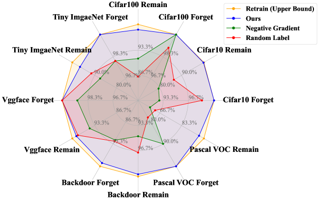
Figure 1: Performance comparison of our method with previous works and retraining (i.e., the upper bound set to 100%) across image classification, data poisoning, face recognition and semantic segmentation, evaluated on forgetting and remaining performance.

In this work, we aim to explore a general unlearning solution for any class-centric tasks, which could not be implemented by existing works as shown in Fig 1. To achieve it, we first propose a theoretical framework to derive the general form of unlearning loss and decouple the unlearning loss into two components: forgetting loss and retention loss, which serve as optimization objectives for forgetting and knowledge retention, respectively. Based on our theoretical framework, we reformulate previous re-label based methods [21, 10, 8] (i.e., a prominent category of unlearning techniques that achieve unlearning by assigning incorrect labels to forget samples.) and observe that they implicitly optimize the forgetting term but lack explicit supervision over the retention term. This limitation hinders the ability to effectively retain knowledge of remaining classes and therefore disturbs the distribution of pre-trained model [16, 10]. To address this, we further refine the retention loss by leveraging “dark knowledge” [68], i.e., the relative magnitudes of the probabilities for the remaining classes. By applying a masking strategy that separates forgetting logits from retention logits, we develop a post-hoc decoupled distillation unlearning method. This approach simultaneously optimizes both the forgetting and refined retention loss components, enabling effective unlearning while retaining essential knowledge. Combining the theoretical framework with our novel unlearning loss, we propose the Decoupled Distillation to Erase method, termed DELETE.

By only modifying the unlearning loss, without bells and whistles we outperform existing unlearning methods by a large margin across different benchmarks, model architectures, and forgetting settings. Additionally, we apply our unlearning loss to downstream tasks such as face recognition, data poisoning and semantic segmentation, and achieve great performance success both in forgetting the target class and remaining others as shown in Fig 1, highlighting its strong generalization capabilities and promising applications in real-world scenarios. To the best of our knowledge, this work presents the first comprehensive and fair comparison of all existing class-centric unlearning methods that do not rely on remaining data or intervention, evaluated under thorough settings across a wide range of benchmarks.

In summary, our main contributions are as follows:

• We adopt a novel theoretical analysis that decomposes the unlearning loss into a forgetting term and a retention term. This inspires a new perspective on leveraging and preserving knowledge within the model based on logits. Under the analysis framework, we also point out that some previous methods implicitly adapt the forgetting term but lack supervision for the retention loss.

• Motivated by the analysis, we further refine the retention loss using “dark knowledge” and introduce the post-hoc decoupled distillation unlearning method, termed DELETE. By masking to decouple the logits of forgotten and non-forgotten classes, we optimize both the decoupled objectives simultaneously, which leads to both effective unlearning and excellent knowledge preservation.

• Through extensive experiments across a wide range of benchmarks, we demonstrate our method’s SOTA performance. Additionally, we apply it to multiple real-world downstream tasks, such as face recognition, backdoor defense, and semantic segmentation, highlighting its strong generalization capabilities.

2 Related Work

Machine Unlearning. Machine Unlearning is the task of removing the influence of specific data from a pretrained model [3, 20, 7]. This task addresses the “right to be forgotten” [60], which is crucial for privacy protection [3] and enhancing AI safety [35, 42, 19]. Retraining from scratch is a common yet naive approach, as it incurs substantial computational overhead [23, 65]. Some methods explore machine unlearning for traditional machine learning tasks, such as linear regression [2, 39], k-means [20], random forests [4], and SVM [11]. However, these methods typically leverage the convex nature of the problem or other theoretical constraints, so that can’t be adopted on DNN [7, 2, 72, 70, 38, 37, 66, 64, 63, 6, 71].

Unlearning in DNN. The urgent need for fast unlearning methods in DNNs leads to various approaches. Some methods require intervention during the pre-training process. SISA [3] splits the model into multiple sub-models trained independently, and selectively removes these sub-models to unlearn. Unrolling SGD [57] adds extra loss terms during training, while other methods [23, 65] rely on stored gradient information to facilitate and speed up unlearning. However, these designs increase computational overhead, reduce efficiency, and may degrade model performance [67, 41], making them impractical for machine-as-a-service (MaaS) and complex real-world applications [25, 62].

To achieve effective forgetting while preserving unrelated knowledge, other methods attempt to use the remaining data. Fisher Forgetting [21] calculates the Fisher Information Matrix based on remaining data, adding noise to scrub parameters associated with forgetting data. SSD [17] calculates parameter importance for both forgotten and remaining data, then applies weight perturbations to unlearn. Additionally, some methods introduce regularization terms or an extra repair stage to reduce interference with unrelated knowledge [56, 30]. However, in real-world applications, factors such as restricted data access, data expiration policies, storage costs, or privacy concerns may prevent providers from storing remaining data [32, 8, 1]. In order to address these challenges, unlearning should ideally be performed without relying on such data. In these cases, the above methods become unusable or suffer from observable performance degradation [17, 56, 51].

Therefore, a stricter and more practical machine unlearning scenario needs to be explored. Our method does not interfere with the pre-training process, or rely on remaining data, making it readily applicable in real-world scenarios.

Knowledge Distillation. Knowledge distillation [27], initially proposed by Hinton et al., is a technique that transfers knowledge from a teacher model to a student model. FitNets [44] further advances this approach by incorporating intermediate features to better align teacher and student models. Decoupled knowledge distillation [68] separate the logits into TCKD and NCKD components, enhancing model capability and generalization.

In recent years, knowledge distillation has been applied across various vision tasks, including machine unlearning [55, 61, 40, 46, 45, 22]. Bad Teacher [12] initializes a pair of competent and incompetent teacher models, using knowledge distillation to selectively unlearn while retaining unrelated knowledge. SCRUB [30] leverages the teacher model’s outputs on remaining data to preserve knowledge. Our approach decouples the unlearning loss into two distinct components and incorporates mask to guide the distillation process. Unlike previous methods, we achieve selective forgetting without access to remaining data.

3 Problem Definition for Machine Unlearning

We now define the notion of class-centric machine unlearning. Let the dataset be denoted as $\mathcal{D}=\{\mathbf{x}_{i},y_{i}\}_{i=1}^{N}\subseteq\mathcal{X}\times\mathcal{Y}$, consisting of $N$ data points. $\mathbf{x}\in\mathcal{X}\subset\mathbb{R}^{d}$ represents the input image, and $y\in\mathcal{Y}=\{1,\cdots,K\}$ is the ground truth label of the image. Let the original classification model trained on the dataset $\mathcal{D}$ be denoted as $f_{\theta_{\mathrm{o}}}:\mathcal{X}\rightarrow\mathcal{Y}$, where $\theta_{\mathrm{o}}$ represents the model parameters.

In machine unlearning, the original dataset is divided into two non-overlapping subsets, $\mathcal{D}_{\mathrm{f}}$ and $\mathcal{D}_{\mathrm{r}}$. The goal of machine unlearning is to erase the knowledge related to $\mathcal{D}_{\mathrm{f}}$ from the model while preserving knowledge related to $\mathcal{D}_{\mathrm{r}}$ remains unaffected. Some existing methods use all or part of $\mathcal{D}_{\mathrm{r}}$ during unlearning to preserve the model’s related knowledge. However, due to privacy concerns and restricted data access in real-world applications [32, 8, 1], we adopt a stricter machine unlearning setting: during unlearning, only the data from $\mathcal{D}_{\mathrm{f}}$ can be used.

As a consequence, the unlearning algorithm trains the model parameters $\theta_{\mathrm{o}}$ on $\mathcal{D}_{\mathrm{f}}$ to obtain new parameters $\theta$. The unlearned model $f_{\theta}$ is required to exhibit incorrect classification on $\mathcal{D}_{\mathrm{f}}$, while maintaining high classification accuracy on $\mathcal{D}_{\mathrm{r}}$. The model $f_{\theta^{\star}}$, retrained on $\mathcal{D}_{\mathrm{r}}$, is typically regarded as the upper bound for machine unlearning [10, 58]. The output of the unlearned model $f_{\theta}$ should be as close as possible to this target model $f_{\theta^{\star}}$.

4 Theoretical Analysis and Method

In this section, we first present a theoretical analysis framework to explore the general form of unlearning loss and decompose it into forgetting and retention losses. Based on the theoretical analysis, we show that re-label unlearning methods are a special case of unlearning loss. Then we suggest a forgetting condition  on the forgetting loss derived from experimental observations; while re-label methods also implicitly satisfy this, they lack supervision on the remaining classes. Therefore, we introduce a retention condition for the retention loss. By combining both conditions, we finally propose a mask distillation unlearning method.

4.1 Theoretical Analysis

1) Decoupling Unlearning Loss. In this section, inspired by DKD [68], we propose the unlearning loss and decompose it into two parts: the forgetting loss and the retention loss. For a classification sample $\mathbf{x}\in\mathcal{D}_{\mathrm{f}}$ from class $u$ to be unlearned, let the target probability distribution output be $\mathbf{p}\in\mathbb{R}^{K}$, and the output of the actual unlearning model $f_{\theta}$ be $\mathbf{q}\in\mathbb{R}^{K}$. Typically, the unlearning loss should reduce KL divergence, given by $\mathcal{L}=\mathrm{KL}(\mathbf{p}\|\mathbf{q})$.

Let $p_{i}$ denote the $i$-th component of the probability distribution for the target $\mathbf{p}$. Specifically, $p_{u}$ and $p_{\backslash u}=\sum_{i\neq u}p_{i}$ denote the probabilities corresponding to the forgetting class and the sum for all other classes, respectively. We denote the binary-class probabilities as $\mathbf{p}^{(b)}=[p_{u},p_{\backslash u}]$. Similarly, the predicted probabilities $q_{u}$, $q_{\backslash u}$ and the binary-class distribution $\mathbf{q}^{(b)}=[q_{u},q_{\backslash u}]$ are defined. For all classes $i\neq u$, we define $\hat{\mathbf{p}}$ and $\hat{\mathbf{q}}$ as the re-normalized probability distributions over these $K-1$ classes, i.e., each element satisfies $\hat{p}_{i}=\frac{p_{i}}{\sum_{i\neq u}p_{i}}$ and $\hat{q}_{i}=\frac{q_{i}}{\sum_{i\neq u}q_{i}}$ .

The unlearning loss function, which reduces the gap between the model’s predicted distribution and the target distribution, can be decomposed into two parts:

$$\mathcal{L}=p_{u}\log\left(\frac{p_{u}}{q_{u}}\right)+\sum_{i\neq u}p_{i}\log\left(\frac{p_{i}}{q_{i}}\right).$$ (1)

For the second term, leveraging the identities $p_{i}=\hat{p}_{i}\cdot p_{\backslash u}$ and $q_{i}=\hat{q}_{i}\cdot q_{\backslash u}$ for $i\neq u$, we have:

$$\sum_{i\neq u}p_{i}\log\left(\frac{p_{i}}{q_{i}}\right) =p_{\backslash u}\sum_{i\neq u}\hat{p}_{i}\log\left(\frac{\hat{p}_{i}\cdot p_{\backslash u}}{\hat{q}_{i}\cdot q_{\backslash u}}\right)$$

$$=p_{\backslash u}\sum_{i\neq u}\hat{p}_{i}\left(\log\left(\frac{\hat{p}_{i}}{\hat{q}_{i}}\right)+\log\left(\frac{p_{\backslash u}}{q_{\backslash u}}\right)\right)$$

$$=p_{\backslash u}\log\left(\frac{p_{\backslash u}}{q_{\backslash u}}\right)+p_{\backslash u}\sum_{i\neq u}\hat{p}_{i}\log\left(\frac{\hat{p}_{i}}{\hat{q}_{i}}\right).$$

Substituting this result into the equation Eq. 1, the loss function becomes:

$$\mathcal{L} =p_{u}\log\left(\frac{p_{u}}{q_{u}}\right)+p_{\backslash u}\log\left(\frac{p_{\backslash u}}{q_{\backslash u}}\right)+p_{\backslash u}\sum_{i\neq u}\hat{p}_{i}\log\left(\frac{\hat{p}_{i}}{\hat{q}_{i}}\right)$$ (2)

$$=\mathrm{KL}(\mathbf{p}^{(b)}\|\mathbf{q}^{(b)})+p_{\backslash u}\mathrm{KL}(\hat{\mathbf{p}}\|\hat{\mathbf{q}}).$$

Thus, we decouple the original loss function into two components: one focused on enforcing forgetting of the target class, and the other supervising the remaining classes. The former arises from the fact that $\mathbf{p}^{(b)}=[p_{u},p_{\backslash u}]=[p_{u},1-p_{u}]$ depends only on the probability of the forgotten class, $p_{u}$, and similarly, $\mathbf{q}^{(b)}$ depends on $q_{u}$. We refer to these components as the forgetting loss and retention loss.

2) Rethinking Re-label Unlearning Method. In this part, we demonstrate that re-label unlearning methods, a common approach within unlearning tasks, represent a special case of the previously established theoretical framework. This allows us to leverage the conclusions drawn in Eq. 2.

Re-label methods assign a fixed incorrect label $r\neq u$ to sample $\mathbf{x}$ , as a form of supervised unlearning. For example, random label assigns a randomly selected label to $\mathbf{x}$ [21]. Some methods use adversarial attacks to derive replacement labels, by attacking $\mathbf{x}$ against the frozen model $f_{\theta_{\mathrm{o}}}$ [10, 8]. The unlearning loss $\mathcal{L}_{\mathrm{re-label}}$ is defined as the cross-entropy loss between $\mathbf{x}$ and the incorrect label $r$, formulated as:

$$\mathop{\arg\min}\limits_{\theta}\mathcal{L}_{\mathrm{re-label}} =\mathop{\arg\min}\limits_{\theta}-\log(q_{r}).$$ (3)

We then demonstrate that this is equivalent to the KL-divergence between the one-hot vector of class $r$ and the model’s output. Let the one-hot vector for class $r$ be denoted as $\mathbf{e}^{r}$. When the target output distribution $\mathbf{p}:=\mathbf{e}^{r}$, note the fact that target $\mathbf{p}$ is independent of the optimization parameter $\theta$ and the properties of one-hot vectors. In this case, we have:

$$\mathop{\arg\min}\limits_{\theta}\mathcal{L}_{\mathrm{re-label}} =\mathop{\arg\min}\limits_{\theta}-\log(q_{r})+\log(p_{r})$$

$$=\mathop{\arg\min}\limits_{\theta}\log\left(\frac{p_{r}}{q_{r}}\right)$$

$$=\mathop{\arg\min}\limits_{\theta}\sum_{i=1}^{K}p_{i}\log\left(\frac{p_{i}}{q_{i}}\right).$$

By transforming the re-label unlearning loss Eq. 3 into a KL-divergence form as in Eq. 1, we enable further discussion within the decomposition framework introduced earlier. In other words, re-label methods represent a special case of Eq. 2, where the target distribution is set as a one-hot vector.

3) Implicit Forgetting Condition in Re-labeling.While the target distribution is not accessible during unlearning, we can approximate $\mathbf{p}$ by observing the probability distributions generated by the retrain model, which is typically considered the gold standard for machine unlearning [10, 58]. As shown in the Tab. 1 in the subsequent experiments, after unlearning, the probability of the forgotten class $p_{u}$ approaches 0. Previous re-label methods implicitly apply this approximation by using a one-hot target, where $p_{u}$ is set as $p_{u}:=e_{u}=0$.

Based on these observations, we formally adopt the forgetting condition $p_{u}=0$ in forgetting loss from Eq. 2, as an approximation of target distribution. Consequently, we obtain $p_{\backslash u}=1-p_{u}=1$, leading to $\mathbf{p}^{(b)}=[p_{u},p_{\backslash u}]=[0,1]$, which we denote as $\mathbf{e}^{(b)}=[0,1]$. The loss function in Eq. 2 can be further expressed as:

It suggests that the loss function should not only enforce forgetting the target class via the first term, but also supervise predictions for remaining classes via the second and third terms. This structure helps maintain the model’s predictions for other classes before and after unlearning, preventing excessive forgetting.

However, re-label unlearning methods lack this supervision for unrelated classes $i\neq u,r$. Recall re-label methods are equivalent to using a one-hot vector for supervision. The corresponding element in the target distribution is assigned $p_{i}:=0$, (i.e., $\hat{p}_{i}:=0$), transforming Eq. 4 into:

$$\mathcal{L}_{\textrm{re-label}}=\mathrm{KL}(\mathbf{e}^{(b)}\|\mathbf{q}^{(b)})+p_{\backslash u}\hat{p}_{r}\log\left(\frac{\hat{p}_{r}}{\hat{q}_{r}}\right).$$

As a result, the model’s prediction for other classes is left unsupervised, which would otherwise serve as the third term in Eq. 4. This indicates a lack of supervision for the predictions of non-forgetting classes in the retention loss. Thus, some methods leverage remaining data to preserve performance on retained classes [16].

4.2 Mask Distillation Method

Previous work neglected the supervision of remaining classes, hindering the preservation of predictions for other classes. However, when forgetting specified classes, it is important to keep the predictions for other classes unchanged [10]. Additionally, preserving the relative magnitudes of the model’s outputs for other classes, which reflect its “dark knowledge”, also plays a crucial role [68]. Thus, we aim to further retain the relative magnitudes of the non-forgotten outputs on retention loss, under the forgetting condition. This motivates the use of distillation based on the original model’s logits, rather than one-hot supervision, which tends to be overly rigid.

To summarize, our goal is to approximate the target distribution using three key observations and conditions, building further on the Sec. 4.1:

• forgetting condition: The probability output for the unlearning class, $p_{u}$, approaches zero , i.e., $p_{u}=0$, as discussed in Sec. 4.1.

• retaining condition: The relative magnitude for the remaining classes remain unchanged, i.e., for $i\neq u$, $p_{i}\propto\mathrm{Softmax}(f_{\theta_{\mathrm{o}}}(\mathbf{x}))_{i}$.

• probability property: The target probability distribution must satisfy the basic property of a probability distribution, i.e., $\sum_{i=1}^{k}p_{i}=1$.

This inspires us to supervise the current unlearn model $f_{\theta}$ leveraging the variant of distribution predicted by the frozen original model $f_{\theta_{\mathrm{o}}}$. By applying a mask and vector normalization to the model output, we obtain an approximate target distribution that satisfies the above conditions.

Let $\mathbf{z}(\mathbf{x};\theta_{\mathrm{o}})=f_{\theta_{\mathrm{o}}}(\mathbf{x})$ (simplified as $\mathbf{z}$ hereafter) represent the logits of the frozen original model for $\mathbf{x}$, where $\mathrm{Softmax}(\mathbf{z})$ represents the corresponding probability distribution. We introduce $\mathrm{Mask}_{u}(\cdot)$ as a masking function applied to $\mathbf{v}\in\mathbb{R}^{K}$, which sets the probability of class $u$ to zero while leaving the other dimensions unchanged. Recalling that $\mathbf{e}^{u}$ is the $u$-th column of the identity matrix $I$, this masking function is defined as the Hadamard product:

$$\mathrm{Mask}_{u}(\mathbf{v})=(\mathbf{1}-\mathbf{e}^{u})\odot\mathbf{v}.$$

The $\mathrm{Normalize}(\cdot)$ function normalizes the vector to ensure that the sum of its elements equals 1, which is achieved by dividing each element by the total sum of all.

By applying the masking and normalization function to process the frozen model’s output as the target, we have:

$$\mathcal{L}=\mathrm{KL}\left(\mathrm{Normalize}(\mathrm{Mask}_{u}(\mathrm{Softmax}(\mathbf{z})))\,\middle\|\,\mathbf{q}\right).$$ (5)

The target in Eq. 5 satisfies all these conditions. By masking out the probability for the target class, we satisfy forgetting condition. The probabilities for the other classes remain after the masking process, and after normalization, they are proportional to the original model’s output probabilities, satisfying retaining condition. Clearly, the normalize function ensures the probability property.

Compared to explicitly specifying a one-hot target vector, the masking design allows for a more fine-grained utilization of the logits for the decoupled forgetting and non-forgetting components. This approach not only enables effective unlearning but also preserves knowledge of the non-forgotten classes, as shown later in Sec. 5.3.

Moreover, we demonstrate that, with a carefully designed mask function $\mathrm{Mask}_{u}^{\prime}(\cdot)$, the masking and softmax steps can be interchanged. This reordering allows the softmax vector to naturally sum to 1, reducing the need for normalization while achieving equivalent results. Further details are provided in the Appendix. The resulting loss function, derived from Eq. 5, is as follows:

$$\mathcal{L} =\mathrm{KL}\left(\mathrm{Softmax}(\mathrm{Mask}_{u}^{\prime}(\mathbf{z}))\,\middle\|\,\mathbf{q}\right).$$

For clarity, the Algorithm 1 provides the final method.

Algorithm 1 Pseudocode of DELETE in a PyTorch-like style.

⬇

# unlearn_model: the classification model to unlearn

# images: the input images to forget (N, 3, H, W)

# labels: the corresponding labels (N, K)

# Initialize the frozen model with unlearn model

frozen_model = copy(unlearn_model)

# Disable gradient computation for the frozen model

frozen_model.params.require_grad_(False)

for images, labels in loader:

# Create a decoupled distillation mask

mask = zeros((N, K))

mask[arange(N), labels] = -float("inf")

# Compute soft targets using the frozen model

frozen_outputs = frozen_model.forward(images)

masked_outputs = mask + frozen_outputs

soft_targets = softmax(masked_outputs, dim=1)

# Forward pass through the unlearn model

logits = unlearn_model.forward(images)

loss = KLDivLoss(softmax(logits, dim=1), soft_targets)

# Update the unlearn model

loss.backward()

update(unlearn_model.params)

5 Experiments

5.1 Experimental Setup

Considering privacy requirements, restricted access, computational constraints, and other real-world limitations as mentioned before, we impose two strict constraints in our experiments: (i) No access to the remaining data; (ii) No intervention during the pre-training phase. Additional implementation details are provided in the appendix.

Datasets. To evaluate the performance on class-centric unlearning task, we use CIFAR-10, CIFAR-100 [29], and Tiny ImageNet [31] datasets. For both single-class and multi-class forgetting tasks, we randomly select a set of classes, then unlearn the same selected classes across methods.

Models. We adopt ResNet-18 [26] as the primary architecture for forgetting experiments. Additionally, we evaluate methods on ViT-s [14], Swin-T [36], and VGGNet-16 [53] to assess effectiveness across different model structures.

Baselines. In our experiments, we compare the following baselines : Random Label, Negative Gradient, Finetune, Fisher Forgetting [21], Boundary Shrink [10], Boundary Expand [10], Learn to Unlearn [8], Bad Teacher [12], Saliency Unlearn [16], SCRUB [30] and Influence Unlearn [28].

Additionally, we include the performance of the original model and the retrained model, with the latter often considered the gold standard in machine unlearning [10, 58].

Metrics. We employ the following accuracy to evaluate effectiveness:$\textbf{Acc}_{\textbf{f}}$ on the forget training data $\mathcal{D}_{\mathrm{f}}$, $\textbf{Acc}_{\textbf{r}}$ on the remain training data $\mathcal{D}_{\mathrm{r}}$, $\textbf{Acc}_{\textbf{ft}}$ on the forget test data $\mathcal{D}_{\mathrm{ft}}$, and $\textbf{Acc}_{\textbf{rt}}$ on the remain test data $\mathcal{D}_{\mathrm{rt}}$.

We further use H-Mean as an overall performance measure of model forgetting and retention. Similar to gs-lora [69], $\mathrm{H}$-$\mathrm{Mean}$ is computed as the harmonic mean of $\mathrm{Acc}_{\mathrm{rt}}$ and $\mathrm{Drop}_{\mathrm{ft}}$, where $\mathrm{Drop}_{\mathrm{ft}}$ represents the performance drop on the forget test data after unlearning.

What’s more, we employ MIA, the membership inference attack [52] success rate, as another indicator of forgetting effectiveness. MIA measures the proportion of samples in $\mathcal{D}_{\mathrm{f}}$ that the unlearn model may still “memorize”, revealing potential remnants of the forget data [16].

Metrics associated with $\mathrm{Acc}_{\mathrm{f}}$, $\mathrm{Acc}_{\mathrm{ft}}$, and MIA should approach zero to indicate effective forgetting, while metrics such as $\mathrm{Acc}_{\mathrm{r}}$, $\mathrm{Acc}_{\mathrm{rt}}$, and H-Mean are expected to align with original model’s, demonstrating retention of knowledge in the remaining classes [10, 16, 69].

5.2 Results and Comparisons

Performance on Different Datasets.

Table 1: Performance comparison of single-class forgetting across different unlearning methods on CIFAR-10 and CIFAR-100 datasets. Gray indicates methods with remain data or intervention, and bold indicates the single best result among methods w/o remain data or intervention (if multiple, results are not in bold). The same notation applies hereafter.

Method		CIFAR-10						CIFAR-100
		$\mathrm{Acc}_{\mathrm{f}}\downarrow$	$\mathrm{Acc}_{\mathrm{r}}\uparrow$	$\mathrm{Acc}_{\mathrm{ft}}\downarrow$	$\mathrm{Acc}_{\mathrm{rt}}\uparrow$	$\mathrm{H\text{-}Mean}\uparrow$	$\mathrm{MIA}\downarrow$	$\mathrm{Acc}_{\mathrm{f}}\downarrow$	$\mathrm{Acc}_{\mathrm{r}}\uparrow$	$\mathrm{Acc}_{\mathrm{ft}}\downarrow$	$\mathrm{Acc}_{\mathrm{rt}}\uparrow$	$\mathrm{H\text{-}Mean}\uparrow$	$\mathrm{MIA}\downarrow$
Original Model		100	100	97.00	95.31	-	99.08	100	99.98	67.00	77.79	-	98.00
Retrain Model		0	100	0	95.20	96.09	0	0	99.97	0	77.64	71.93	0
Random Label		00.10	90.66	01.60	82.18	88.30	0	01.20	96.60	01.00	66.99	66.49	0
Negative Gradient		11.12	83.94	07.20	75.52	82.04	07.44	02.20	97.80	0	70.66	68.78	01.20
Boundary Shrink		00.28	90.34	04.50	84.56	88.35	00.22	01.40	96.48	0	68.46	67.72	0
Boundary Expand		11.32	90.74	15.00	79.37	80.66	00.86	02.40	98.59	01.00	71.69	68.73	0
Influence Unlearn		01.04	99.58	00.60	93.21	94.78	0	0	97.83	0	71.03	68.96	0
Learn to Unlearn		12.36	96.49	08.60	90.02	89.20	07.56	01.60	97.70	0	70.29	68.61	00.40
Bad Teacher		01.98	92.23	18.80	87.13	82.42	00.52	01.60	98.46	03.00	71.38	67.49	00.20
Bad Teacher		00.34	99.99	00.30	94.98	95.83	0	00.40	99.98	0	77.63	71.92	0
Saliency Unlearn		09.98	79.19	10.50	70.18	80.53	11.70	01.20	88.07	03.00	59.73	61.79	01.00
Saliency Unlearn		00.84	99.73	00.10	93.91	95.38	00.02	00.80	99.21	0	74.27	70.45	0
Fisher Forget		68.94	57.33	68.30	59.73	38.77	59.50	66.00	74.52	37.00	54.68	38.74	68.60
SCRUB		0	99.92	0	94.94	95.96	0	0	99.95	0	77.41	71.83	0
Finetune		00.12	99.53	0	93.83	95.39	0	0	99.30	0	74.15	70.39	0
Ours		0	100	0	95.03	96.00	0	0	99.97	0	76.57	71.47	0

In this part, we discuss the single-class forgetting performance across various datasets. Although our experimental setup does not allow access to remaining data or intervention, we still compare several methods that have these, marking them with gray.

Using CIFAR-10 as an example in Tab. 1, although all methods achieve varying degrees of forgetting in $\mathrm{Acc}_{\mathrm{ft}}$, some methods like Negative Gradient maintain $\mathrm{Acc}_{\mathrm{f}}$ and $\mathrm{Acc}_{\mathrm{ft}}$ around 10%, indicating incomplete forgetting. In contrast, our method achieves complete forgetting in $\mathrm{Acc}_{\mathrm{ft}}$ while maintaining an excellent $\mathrm{Acc}_{\mathrm{rt}}$, with a minimal gap of only 0.17% compared to the retrain model. When experiments are extended to larger datasets such as CIFAR-100 and Tiny ImageNet (Tab. 1 and Appendix), the performance of some methods fluctuates significantly. Notably, our method consistently outperforms all other methods across all datasets and metrics.

Performance on Different Models.

Table 2: Performance comparison across different models.

	$\mathrm{Acc}_{\mathrm{f}}\downarrow$	$\mathrm{Acc}_{\mathrm{r}}\uparrow$	$\mathrm{Acc}_{\mathrm{ft}}\downarrow$	$\mathrm{Acc}_{\mathrm{rt}}\uparrow$	$\mathrm{H\text{-}Mean}\uparrow$	$\mathrm{MIA}\downarrow$
VGGNet-16
00Original Model	99.94	99.94	91.20	92.02	-	99.88
00Retrain Model	0	99.71	0	92.49	91.84	0
00Boundary Shrink	06.68	91.15	06.80	82.79	83.59	02.84
00Ours	0	99.66	0	92.08	91.64	0
Swin-T
00Original Model	85.00	86.58	82.70	82.68	-	82.94
00Retrain Model	0	86.41	0	82.77	82.73	0
00Boundary Shrink	05.54	62.94	02.50	58.18	67.44	11.36
00Ours	0	85.37	0	83.09	82.89	0
ViT-S
00Original Model	90.50	90.57	72.70	75.73	-	84.60
00Retrain Model	0	92.42	0	76.44	74.52	0
00Boundary Shrink	01.84	73.16	01.70	65.59	68.19	01.66
00Ours	0	90.74	0	77.21	74.89	0

To evaluate effectiveness across various models, we further conduct single-class unlearning experiments with VGGNet-16, Swin-T, and Vit-S, as shown in Tab. 2. A full comparison of methods is provided in the Appendix. At the same performance of $\mathrm{Acc}_{\mathrm{ft}}$, our method shows a maximum performance gap of only 0.77% in $\mathrm{Acc}_{\mathrm{rt}}$ compared to the retrain model, demonstrating consistently excellent results across different architectures while Boundary Shrink shows limited performance, validating the robustness of DELETE.

Performance with Frozen Linear Classifier.

Table 3: Performance comparison with frozen linear classifier.

Method	$\mathrm{Acc}_{\mathrm{f}}\downarrow$	$\mathrm{Acc}_{\mathrm{r}}\uparrow$	$\mathrm{Acc}_{\mathrm{ft}}\downarrow$	$\mathrm{Acc}_{\mathrm{rt}}\uparrow$	$\mathrm{H\text{-}Mean}\uparrow$	$\mathrm{MIA}\downarrow$
Original Model	100	100	97.00	95.31	-	99.08
Retrain Model	0	100	0	95.12	96.05	0
Random Label	00.82	93.60	06.90	85.51	87.75	0
Negative Gradient	19.20	87.83	15.00	79.37	80.66	13.88
Boundary Shrink	01.12	87.97	09.30	82.43	84.98	01.36
Boundary Expand	58.44	32.02	69.60	39.13	32.23	66.62
Bad Teacher	04.14	86.26	24.80	81.51	76.57	02.14
Saliency Unlearn	10.58	85.95	11.20	76.14	80.68	03.78
Influence Unlearn	00.40	99.61	00.20	93.59	95.17	00.20
Learn to Unlearn	21.00	97.86	17.60	91.09	84.84	15.54
Ours	0	100	0	95.44	96.21	0

A key concern in machine unlearning is whether knowledge of the target class is truly forgotten. Studies suggest that forgetting often occurs in the model’s linear classifier [8]. However, merely modifying classifier to misclassify without erasing knowledge at the feature level doesn’t fulfill the goal of machine unlearning [21]. Incomplete forgetting within the feature extractor could also introduce risks of privacy leakage.

To address this, we freeze the model’s linear classifier and train only the feature extractor to forget. Results, shown in Tab. 3, demonstrate that our method consistently outperforms existing approaches across all metrics. Boundary Expand shows a significant drop in overall performance, suggesting such methods achieve unlearning primarily at the classifier level rather than at the feature level.

Performance on Multi-Class Forgetting.

Table 4: Comparison of the classification accuracy of multi-class forgetting across methods on CIFAR-100 dataset.

Method		1 Class			2 Classes			5 Classes			10 Classes			20 Classes
		$\mathrm{Acc}_{\mathrm{ft}}\downarrow$	$\mathrm{Acc}_{\mathrm{rt}}\uparrow$	$\mathrm{H\text{-}Mean}\uparrow$	$\mathrm{Acc}_{\mathrm{ft}}\downarrow$	$\mathrm{Acc}_{\mathrm{rt}}\uparrow$	$\mathrm{H\text{-}Mean}\uparrow$	$\mathrm{Acc}_{\mathrm{ft}}\downarrow$	$\mathrm{Acc}_{\mathrm{rt}}\uparrow$	$\mathrm{H\text{-}Mean}\uparrow$	$\mathrm{Acc}_{\mathrm{ft}}\downarrow$	$\mathrm{Acc}_{\mathrm{rt}}\uparrow$	$\mathrm{H\text{-}Mean}\uparrow$	$\mathrm{Acc}_{\mathrm{ft}}\downarrow$	$\mathrm{Acc}_{\mathrm{rt}}\uparrow$	$\mathrm{H\text{-}Mean}\uparrow$
Original Model		67.00	77.79	-	78.00	77.66	-	76.80	77.72	-	78.80	77.54	-	77.40	77.74	-
Retrain Model		0	77.64	71.93	0	78.09	78.04	0	78.63	77.70	0	79.08	78.94	0	80.35	78.85
Random Label		1.00	66.99	66.49	4.00	65.97	69.75	2.80	63.51	68.35	3.10	59.97	66.92	4.45	59.35	65.45
Negative Gradient		0	70.66	68.78	1.50	69.96	73.08	0.20	68.97	72.59	2.10	67.11	71.59	3.10	40.60	52.51
Boundary Shrink		0	68.46	67.72	1.00	60.10	67.51	0.40	63.68	69.46	0.50	59.19	67.42	3.90	61.90	67.20
Boundary Expand		1.00	71.69	68.73	0.50	69.00	73.00	2.80	69.03	71.43	2.70	64.79	69.99	5.80	62.59	66.79
Influence Unlearn		0	71.03	68.96	0	67.84	72.57	2.20	62.33	67.92	0	37.56	50.87	20.20	43.77	49.59
Learn to Unlearn		0	70.29	68.61	0.50	69.35	73.20	0	58.80	66.61	1.80	66.56	71.40	20.65	64.90	60.55
Bad Teacher		3.00	71.38	67.49	0	59.48	67.49	0.80	62.61	68.66	0.50	58.17	66.75	3.10	55.07	63.26
Saliency Unlearn		3.00	59.73	61.79	2.50	56.60	64.70	3.00	64.64	68.92	3.20	53.84	62.89	6.05	62.31	66.52
Ours		0	76.57	71.47	0	76.78	77.39	0	77.76	77.28	0.50	77.61	77.95	1.20	79.30	77.72

Building on single-class forgetting in CIFAR-100, we further experiment with forgetting multiple classes. As shown in Tab. 4, the results indicate that some methods suffer significant performance drops as forgetting class number increases. When forgetting 20 classes, none of the other methods achieve both an $\mathrm{Acc}_{\mathrm{ft}}$ of 0% and an $\mathrm{Acc}_{\mathrm{rt}}$ above 65%, as they do in single-class forgetting. In contrast, our method demonstrates exceptional multi-class forgetting capability, showing the power of our novel loss function.

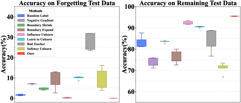
Figure 2: Boxplot comparison of accuracy on $\mathcal{D}_{\textrm{ft}}$ (left) and $\mathcal{D}_{\textrm{rt}}$ (right) across 5 runs, illustrating accuracy distributions and stability. Ours consistently achieves the lowest $\textrm{Acc}_{\textrm{ft}}$ and the highest $\textrm{Acc}_{\textrm{rt}}$, demonstrating stable performance across executions.

Performance Comparison of Stability and Insensitivity. In this part, we discuss the stability and learning rate insensitivity of different methods. To evaluate the stability of each method, we conduct five repeated single-class forgetting runs. As shown in Fig. 2, some methods exhibit considerable performance variance, indicated by the width of the boxplots. Meanwhile, ours demonstrate excellent stability.

Moreover, an promising method is expected to demonstrate insensitivity to the learning rate across varying numbers of forgetting classes, i.e., achieving strong performance with a fixed learning rate. Otherwise, a different number of unlearning classes would require frequent adjustments, resulting in additional computational overhead and unstable performance. As shown in Fig. 3, our method achieves effective forgetting while preserving high accuracy on the remaining data. In contrast, all other methods exhibit varying degrees of performance degradation in $\textrm{Acc}_{\textrm{rt}}$ or $\textrm{Acc}_{\textrm{ft}}$, resulting in a noticeable performance gap compared to ours.

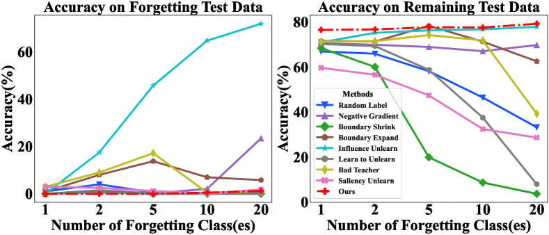
Figure 3: Accuracy comparison on $\mathcal{D}_{\textrm{ft}}$ (left) and $\mathcal{D}_{\textrm{rt}}$ (right) across multiple forgetting classes with a fixed learning rate. Ours achieves superior $\textrm{Acc}_{\textrm{ft}}$ and $\textrm{Acc}_{\textrm{rt}}$, whereas all other methods exhibit varying degrees of performance degradation.

5.3 Ablation Study

In this part, we conduct ablation studies to validate the effectiveness of the forgetting and retention conditions.

For the forgetting condition, the output on forget class is required to approach 0, enforcing the erasure of target class. To validate this, we define $p_{u}=\alpha\cdot\mathrm{Softmax}(f_{\theta_{\mathrm{o}}}(\mathbf{x}))_{u}$, where setting $\alpha=0$ represents our default setting. Increasing $\alpha$ deviates from this, and is expected to gradually weaken the forgetting effect.

Similarly, the retention condition is designed to preserve non-target classes knowledge. It’s implemented with $p_{i}\propto\mathrm{Softmax}(f_{\theta_{\mathrm{o}}}(\mathbf{x})/T)_{i}$, where $T=1$ is our default setting. Increasing $T$ deviates from the retention condition and is anticipated to reduce the retention effect.

Table 5: Ablation study on forgetting and retention conditions, with varying values of $\alpha$ and $T$ respectively.

	$\mathrm{Acc}_{\mathrm{f}}\downarrow$	$\mathrm{Acc}_{\mathrm{r}}\uparrow$	$\mathrm{Acc}_{\mathrm{ft}}\downarrow$	$\mathrm{Acc}_{\mathrm{rt}}\uparrow$	$\mathrm{H\text{-}Mean}\uparrow$
Retrain Model	0	100	0	95.20	96.09
Our Method	0	100	0	95.03	96.00
Effect of varying $\alpha$
00$\alpha=0.25$	41.00	100	37.30	95.49	73.47
00$\alpha=0.50$	91.84	99.99	76.80	95.31	33.33
00$\alpha=0.75$	99.88	99.97	95.00	94.36	03.92
Effect of varying $T$
00$T=5$	0	78.60	0	76.92	85.80
00$T=10$	0	30.13	0	30.38	46.27
00$T=15$	0	17.51	0	18.81	31.51

The experimental results, as shown in Tab. 5, align well with our expectations. When progressively increasing $\alpha$ to violate the forgetting condition, the model’s accuracy on $\mathcal{D}_{\mathrm{ft}}$ steadily rises from 0% to 95.00%. Likewise, increasing $T$ to deviate from the retention condition reduces the model’s accuracy on $\mathcal{D}_{\mathrm{rt}}$, from 95.03% to 18.81%. It is noteworthy that when varying $\alpha$ to validate the forgetting condition, $\text{Acc}_{\text{rt}}$ remains stable, while varying $T$ results in the same stability in $\text{Acc}_{\text{ft}}$. This confirms the validity of our conditions in effectively controlling forgetting without compromising retention, and vice versa.

5.4 Feature Representation Visualization

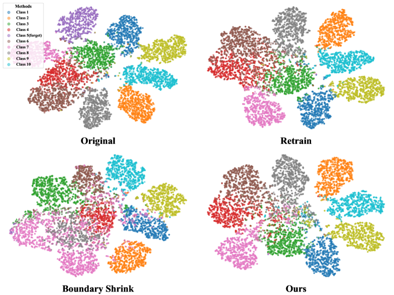
Figure 4: T-SNE visualization of feature representations space.

To investigate the impact of forgetting on model’s feature space, we use t-SNE [59] to visualize the feature distributions. Different colors indicate distinct predicted classes, and triangles are used to mark samples belonging to the forgetting class. As illustrated in Fig. 4, the original model exhibits clear class boundaries. Both ours and retrain model successfully unlearn the forget class samples, marked in purple, while preserving the boundaries of the remaining classes. In contrast, Boundary Shrink causes noticeable boundary degradation in certain classes; for example, the pink dots are dispersed across various regions of the space.

6 Application to Downstream Tasks

6.1 Face Recognition with Unlearning

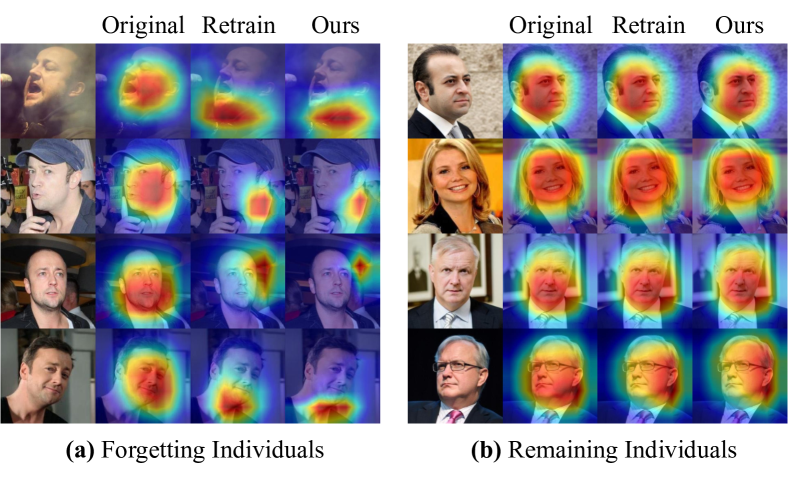
Figure 5: Grad-CAM visualization of face recognition models on forgetting and remaining individuals.

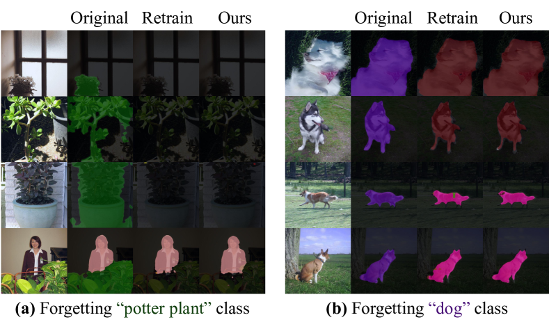
Figure 6: Visualization of unlearning in semantic segmentation.

In this part, we apply machine unlearning to face recognition to achieve the objective of safeguarding individual privacy [5, 10]. As shown in the Appendix, our method outperforms all other methods across all metrics and achieves results closest to the retrain model in quantitative comparisons. To further investigate the forgetting effects, we employ Grad-CAM [49] to visualize model attention areas. The heatmaps highlight areas important to each model’s predictions. In Fig. 5a, which relates to individuals designated for forgetting, the original model focuses on facial regions, while both the retrain model and our model effectively suppress recognition signals associated with these faces. In Fig. 5b, depicting remaining individuals, all three models maintain strong attention on relevant features, indicating robust knowledge retention for non-forgotten classes.

6.2 Backdoor Defense with Unlearning

Data poisoning is a common backdoor attack method. Employing unlearning methods allows us to eliminate the influence of poisoned data and achieve effective defense. We adopt the recovery algorithm [35] and utilize DELETE to unlearn. The quantitative results in the Appendix show that DELETE achieves improved performance. Notably, for 3×3 size, we observe improvements of 6.96% and 4.19% compared to others. Meanwhile, other methods face challenges of insufficient defense and reduced model performance.

6.3 Semantic Segmentation with Unlearning

We compare the segmented output images of the original model, the retrain model, and ours, as illustrated in Fig. 6. Our model achieves segmentation results similar to those of the retrain model, effectively avoiding the segmentation of the target class. Notably, forgetting a class is not the same as merely mis-segmenting it as background. For example, due to the absence of dog training samples, the retrained model may classify dog as other visually similar categories, such as cat or cow in Fig. 6b. Our approach effectively reproduces this behavior. The quantitative comparison results are provided in the Appendix.

7 Conclusion

In this paper, we introduce a novel machine unlearning method DELETE that requires neither access to remaining data nor intervention during training, aligning closely with real-world application constraints. Leveraging a theoretical framework that decomposes unlearning loss into forgetting and retention terms, our method effectively separates the influence of forgotten and retained classes through a masking distillation approach. Extensive experiments demonstrate its state-of-the-art performance across setups. We also apply our method to downstream tasks, including face recognition, backdoor unlearning, and semantic segmentation, demonstrating its real-world potential.

Supplementary Material

This appendix provides supplementary materials that could not be included in the main paper due to space limitations. In Sec. H, we present the reformulation of the loss function Eq. (5). Sec. I provides details on the implementation, baselines, and evaluation metrics. Sec. J provides additional performance comparisons of various methods across different datasets and models. Finally, Sec. K demonstrates the implementation details, quantitative results, and qualitative results of applying our method to downstream tasks, including face recognition, backdoor defense, and semantic segmentation.

H Reformulation

In this section, we reformulate the loss function Eq. (5) in the main paper. We prove that, with an appropriately designed mask $\mathrm{Mask}_{u}^{\prime}(\cdot)$, the masking and softmax steps can be interchanged. After reordering, the resulting softmax vector satisfies the condition that the sum of its elements equals 1, thereby obviating the need for additional normalization.

We define the mask function as $\mathrm{Mask}_{u}^{\prime}(\mathbf{v})=\mathbf{v}+\mathbf{m}^{u}$, where the vector $\mathbf{m}^{u}\in\mathbb{R}^{K}$ is defined as:

$$\mathbf{m}_{i}^{u}=\begin{cases}0&\text{if }i\neq u,\\ -\infty&\text{if }i=u.\end{cases}$$

Next, we prove that interchanging the mask and softmax steps with an appropriately designed mask function results in proportional outcomes, i.e.,

$$\mathrm{Mask}_{u}(\mathrm{Softmax}(\mathbf{z}))\propto\mathrm{Softmax}(\mathrm{Mask}_{u}^{\prime}(\mathbf{z}))$$

This is beacuse, for $i\neq u$, we have:

$$\mathrm{Mask}_{u}(\mathrm{Softmax}(\mathbf{z}))_{i} =\frac{e^{z_{i}}}{\sum_{i}e^{z_{i}}}$$

$$=\frac{e^{z_{i}}}{\sum_{i\neq u}e^{z_{i}}}\times\frac{\sum_{i\neq u}e^{z_{i}}}{\sum_{i}e^{z_{i}}}.$$

Meanwhile,

$$\mathrm{Softmax}(\mathrm{Mask}_{u}^{\prime}(\mathbf{z}))_{i} =\frac{e^{z_{i}}}{e^{-\infty}+\sum_{i\neq u}e^{z_{i}}}$$

$$=\frac{e^{z_{i}}}{\sum_{i\neq u}e^{z_{i}}}.$$

For $i=u$, both element yield 0:

$$\mathrm{Mask}_{u}(\mathrm{Softmax}(\mathbf{z}))_{i}=\mathrm{Softmax}(\mathrm{Mask}_{u}^{\prime}(\mathbf{z}))_{i}=0$$

Thus, for any $i$, combining the two cases above, we obtain the following relationship:

$$\mathrm{Mask}_{u}(\mathrm{Softmax}(\mathbf{z}))_{i}=\mathrm{Softmax}(\mathrm{Mask}_{u}^{\prime}(\mathbf{z}))_{i}\times\frac{\sum_{i\neq u}e^{z_{i}}}{\sum_{i}e^{z_{i}}}.$$

Since the elements of both vectors are proportional by a factor, normalizing these vectors results in identical outputs. Given that the softmax operation ensures the output vector is already normalized (i.e., its elements sum is 1), we conclude:

$$\mathrm{Normalize}(\mathrm{Mask}_{u}(\mathrm{Softmax}(\mathbf{z})))=\mathrm{Softmax}(\mathrm{Mask}_{u}^{\prime}(\mathbf{z})).$$ (S6)

Thus, we can interchange the mask and softmax steps via Eq. S6, thereby simplifying Eq. (5) in the main paper by removing the need for normalization. The final loss function is expressed as:

$$\mathcal{L} =\mathrm{KL}\left(\mathrm{Normalize}(\mathrm{Mask}_{u}(\mathrm{Softmax}(\mathbf{z})))\,\middle\|\,\mathbf{q}\right)$$

$$=\mathrm{KL}\left(\mathrm{Softmax}(\mathrm{Mask}_{u}^{\prime}(\mathbf{z}))\,\middle\|\,\mathbf{q}\right).$$

I Experimental Details

I.1 Implementation Details

Our implementation is based on Python 3.8 and PyTorch 1.13. All experiments are conducted on a system equipped with NVIDIA RTX 4090 GPU and Intel Xeon Gold 6226R CPU. For the image classification unlearning task, we first train the original model from scratch. The optimizer settings are detailed in Tab. S6. The training configurations for different models and datasets during pretraining are provided in Tab. S7. The retrain model follows the same training configurations but is trained exclusively on $\mathcal{D}_{\textrm{r}}$, without access to $\mathcal{D}_{\textrm{f}}$.

Table S6: Optimization settings for image classification.

Config	Value
Optimizer	SGD
Weight Decay	5e-4
Momentum	0.9
Learning Rate Scheduler	Step LR Scheduler
Learning Rate Step	40
Learning Rate Gamma	0.1

Table S7: Pre-training setups for different datasets and models.

Different Datasets	CIFAR-10	CIFAR-100	Tiny ImageNet
	ResNet-18	ResNet-18	ResNet-18
Pretrain Epochs	150	150	150
Pretrain LR	0.1	0.1	0.1
Batch Size	128	128	64
Different Models	VGG-16	Swin-T	ViT-S
	CIFAR-10	CIFAR-10	CIFAR-10
Pretrain Epochs	80	100	150
Pretrain LR	0.01	0.01	0.1
Batch Size	128	64	128

I.2 Baseline Details

Recalling that we compare the unlearning performance of different methods, under the two imposed constraints: (i) No access to the remaining data; (ii) No intervention during the pre-training phase. Under these constraints, certain methods become infeasible. Finetune, Fisher Forget [21], SSD [17], and SISA [3] fail to work due to their reliance on remaining data or intervention in their algorithms. Bad Teacher [12], Saliency Unlearn[16], SCRUB [30], and UNSIR[56] are unable to compute regularization loss or perform additional repair phases.

Nevertheless, to better compare the performance of different methods, we select several well-known approaches and evaluate them under scenarios without the aforementioned constraints. The selected methods include Finetune, Fisher Forget, Bad Teacher, and Saliency Unlearn, with their results marked in gray in the main paper. Specifically, for Bad Teacher and Saliency Unlearn, we also remove the regularization loss that depend on remaining data and test their performance under the imposed constraints. These results are marked in black.

For training-based unlearning methods, we perform unlearning for 20 epochs and search for the optimal learning rate within the range of $[10^{-7},10^{-2}]$. For parameter-scrubbing unlearning methods, we search for the hyperparameter $\alpha$ in the range of $[10^{-8},10^{-5}]$ for Fisher Forget, and in the range of $[10^{-2},10^{2}]$ for Influential Unlearn. All other hyperparameter settings follow the configurations in the responding original papers.

I.3 Mertic Details

Following prior work, we use membership inference attacks (MIA) success rate as a metric to evaluate the forgetting performance of the unlearn model [16]. The MIA implementation is based on a prediction confidence-based attack method [54]. To construct the dataset for training the MIA predictor, we sample a balanced binary classification dataset from $\mathcal{D}_{\textrm{r}}$ and $\mathcal{D}_{\textrm{rt}}$. The input consists of the confidence scores predicted by the model for the images, while the corresponding labels indicate whether each image originates from $\mathcal{D}_{\textrm{r}}$ or $\mathcal{D}_{\textrm{rt}}$.

During the evaluation phase, the confidence scores predicted by $f_{\theta}$ on $\mathcal{D}_{\textrm{f}}$ are used as input to the MIA predictor. The classification results of the MIA predictor are then used to assess how many samples in the forgetting dataset are still memorized by the model after unlearning. The MIA metric is defined as:

$$\textrm{MIA}=\frac{\textrm{TP}}{|\mathcal{D}_{\textrm{f}}|}$$

where it measures the proportion of samples in $\mathcal{D}_{\textrm{f}}$ that the MIA predictor classifies as still being memorized by the model. In other words, it represents the proportion of samples in $\mathcal{D}_{\textrm{f}}$ that were not successfully forgotten.

Note that our MIA evaluation is slightly different from Saliency Unlearn’s [16]. We measure the proportion of samples in $\mathcal{D}_{\textrm{f}}$ that have not been successfully forgotten, whereas Saliency Unlearn measures the proportion of successfully forgotten samples. We adopt this approach to maintain consistency with metrics such as $\textrm{Acc}_{\textrm{f}}$ and $\textrm{Acc}_{\textrm{ft}}$, where lower values indicate better forgetting performance.

J Experimental Results

J.1 Performance on Different Datasets

Table S8: Performance comparison of single-class forgetting across different unlearning methods on Tiny ImageNet dataset. bold indicates the single best result among methods. The same notation applies hereafter.

Method	$\mathrm{Acc}_{\mathrm{f}}\downarrow$	$\mathrm{Acc}_{\mathrm{r}}\uparrow$	$\mathrm{Acc}_{\mathrm{ft}}\downarrow$	$\mathrm{Acc}_{\mathrm{rt}}\uparrow$	$\mathrm{H\text{-}Mean}\uparrow$	$\mathrm{MIA}\downarrow$
Original Model	100	99.98	66.0	64.15	-	99.4
Retrain Model	0	99.98	0	64.42	65.20	0
Random Label	3.2	97.58	2.0	58.84	61.31	0.2
Negative Gradient	7.8	95.36	2.0	56.24	59.87	3.0
Boundary Shrink	5.2	97.49	2.0	57.85	60.77	0.6
Boundary Expand	8.6	98.89	2.0	58.88	61.33	0
Influence Unlearn	12.2	99.36	2	60.30	62.09	1.6
Learn to Unlearn	1.0	85.57	0	50.73	57.37	0.2
Bad Teacher	5.8	98.32	2.0	59.02	61.41	0.2
Saliency Unlearn	6.6	98.80	2.0	59.67	61.76	0.6
Ours	0.4	99.94	0	62.15	64.02	0

In the main paper, we present the results of single-class forgetting on CIFAR-10 and CIFAR-100. Tab. S8 further presents the performance on Tiny ImageNet across various methods for the single-class forgetting task. While most methods achieve some degree of forgetting, several exhibit poor retention of knowledge for the remaining classes. For example, Negative Gradient, Boundary Shrink, Boundary Expand, and Learn to Unlearn show a decline of around 5% in $\mathrm{Acc}_{\mathrm{rt}}$ compared to the original model.

Notably, despite Learn to Unlearn performing well on CIFAR-10 and CIFAR-100, its performance drops significantly on Tiny ImageNet, falling from third place on CIFAR-10 to the lowest rank on Tiny ImageNet. This highlights its fragility and inconsistency across datasets.

In contrast, our method consistently demonstrates strong performance, achieving complete forgetting in $\mathrm{Acc}_{\mathrm{ft}}$ while maintaining excellent $\mathrm{Acc}_{\mathrm{rt}}$. Among all methods, ours is one of only two to surpass 60% in $\mathrm{Acc}_{\mathrm{rt}}$, outperforming the second-best method by nearly 2%. Our method outperforms all other approaches across all performance metrics on Tiny ImageNet. This demonstrates the superior balance of our approach between effective forgetting and retention of unrelated knowledge across various datasets.

J.2 Performance on Different Models

Table S9: Performance comparison of single-class forgetting on VGG-16, across different unlearning methods on CIFAR-10.

Method	$\mathrm{Acc}_{\mathrm{f}}\downarrow$	$\mathrm{Acc}_{\mathrm{r}}\uparrow$	$\mathrm{Acc}_{\mathrm{ft}}\downarrow$	$\mathrm{Acc}_{\mathrm{rt}}\uparrow$	$\mathrm{H\text{-}Mean}\uparrow$	$\mathrm{MIA}\downarrow$
Original Model	99.94	99.94	91.20	92.02	-	99.88
Retrain Model	0	99.71	0	92.49	91.84	0
Random Label	0	96.35	0	88.16	89.65	0
Negative Gradient	00.36	92.11	00.20	83.77	87.24	00.20
Boundary Shrink	06.68	91.15	06.80	82.79	83.59	02.84
Boundary Expand	02.82	84.95	02.10	77.27	82.76	01.38
Influence Unlearn	01.86	93.17	01.60	84.74	87.10	01.30
Learn to Unlearn	03.28	94.10	03.00	85.56	86.86	01.96
Bad Teacher	07.14	90.95	07.20	82.90	83.45	0
Saliency Unlearn	11.24	73.37	10.90	69.09	74.27	0
Ours	0	99.66	0	92.08	91.64	0

Table S10: Performance comparison of single-class forgetting on Swin-T, across different unlearning methods on CIFAR-10.

Method	$\mathrm{Acc}_{\mathrm{f}}\downarrow$	$\mathrm{Acc}_{\mathrm{r}}\uparrow$	$\mathrm{Acc}_{\mathrm{ft}}\downarrow$	$\mathrm{Acc}_{\mathrm{rt}}\uparrow$	$\mathrm{H\text{-}Mean}\uparrow$	$\mathrm{MIA}\downarrow$
Original Model	85.00	86.58	82.70	82.68	-	82.94
Retrain Model	0	86.41	0	82.77	82.73	0
Random Label	03.68	74.86	00.90	70.42	75.68	04.68
Negative Gradient	00.46	74.60	00.10	71.98	76.93	00.22
Boundary Shrink	05.54	62.94	02.50	58.18	67.44	11.36
Boundary Expand	02.58	70.36	01.00	65.67	72.81	03.26
Influence Unlearn	00.04	76.02	0	72.99	77.54	0
Learn to Unlearn	00.52	79.55	00.40	76.50	79.29	00.14
Bad Teacher	08.96	74.77	06.30	68.86	72.43	07.24
Saliency Unlearn	11.16	76.88	08.00	72.40	73.53	12.40
Ours	0	86.68	0	83.61	83.15	0

Table S11: Performance comparison of single-class forgetting on ViT-S, across different unlearning methods on CIFAR-10.

Method	$\mathrm{Acc}_{\mathrm{f}}\downarrow$	$\mathrm{Acc}_{\mathrm{r}}\uparrow$	$\mathrm{Acc}_{\mathrm{ft}}\downarrow$	$\mathrm{Acc}_{\mathrm{rt}}\uparrow$	$\mathrm{H\text{-}Mean}\uparrow$	$\mathrm{MIA}\downarrow$
Original Model	90.50	90.57	72.70	75.73	-	84.60
Retrain Model	0	92.42	0	76.44	74.52	0
Random Label	01.32	77.38	01.80	68.51	69.68	02.24
Negative Gradient	00.38	85.25	00.50	73.34	72.77	00.34
Boundary Shrink	01.84	73.16	01.70	65.59	68.19	01.66
Boundary Expand	08.02	75.86	07.80	67.42	66.14	09.24
Influence Unlearn	00.98	87.09	00.90	75.20	73.46	00.78
Learn to Unlearn	00.46	85.11	00.30	73.20	72.80	00.36
Bad Teacher	06.02	74.66	05.40	67.27	67.28	07.32
Saliency Unlearn	06.22	77.54	05.90	68.46	67.62	07.14
Ours	0	90.74	0	77.21	74.89	0

This part compares the performance of various methods across different models. In Tabs. S9, S10 and S11, we present the forgetting performance of different methods on three distinct models, apart from ResNet-18 discussed in the main paper: VGG-16, Swin-T, and ViT-S.

Remarkably, our method achieves the best results across all 18 metrics on all three models. Among these, it achieves the sole best performance on 14 metrics. For the overall performance metric H-Mean, our method outperforms the second-best by margins of 1.99%, 3.86%, and 1.43% on VGG-16, Swin-T, and ViT-S, respectively. Additionally, on $\textrm{Acc}_{\textrm{rt}}$, which measures the preservation of knowledge for unrelated classes, our method leads by 3.92%, 7.11%, and 1.99% over the second-best on the respective models. These results highlight the strong generalization and consistent performance of our method across different architectures.

In contrast, some other methods exhibit significant performance fluctuations, reflecting their fragility when applied to different models. For example, Boundary Shrink shows a gap of 7.74% in H-Mean compared to the retrain model on ResNet-18, which expands to 15.29% on Swin-T, nearly doubling the performance gap. On the other hand, Influence Unlearn demonstrates relatively stable performance, achieving three second-place and one third-place rankings. However, its H-Mean scores are 1.22% to 5.61% lower than those of our method across all models, further emphasizing our superior performance.

K Application to Downstream Tasks

K.1 Face Recognition with Unlearning

Implementation Details. Face recognition experiments are conducted using the VGGFace2 [5] dataset and the ResNet18 model. To prepare the dataset, we first filter individuals with more than 500 images, and randomly select 110 of them. For each individual, we allocate 400 images for the training set and 100 images for the test set.

The model is pretrained using 100 randomly selected individuals from the training set for 80 epochs to obtain a pretrained model. Subsequently, we fine-tune the model for 40 epochs using 10 other individuals. During the unlearning phase, one of these 10 individuals is randomly chosen, and the unlearning process is performed for 20 epochs. To ensure fairness, all methods are evaluated using the same individuals for the pretraining, fine-tuning, and unlearning stages. The batch size is set to 64 for all training stages, and the learning rate is fixed at 0.01 during both the pretraining and fine-tuning phases.

Qualitative Results.

Table S12: Performance comparison of face recognition task on VGG-Face dataset.

Method	$\mathrm{Acc}_{\mathrm{f}}\downarrow$	$\mathrm{Acc}_{\mathrm{r}}\uparrow$	$\mathrm{Acc}_{\mathrm{ft}}\downarrow$	$\mathrm{Acc}_{\mathrm{rt}}\uparrow$	$\mathrm{H\text{-}Mean}\uparrow$	$\mathrm{MIA}\downarrow$
Original Model	100	100	97.00	99.22	-	100
Retrain Model	0	100	0	98.89	97.94	0
Random Label	0	99.97	0	97.22	97.11	0
Negative Gradient	01.15	98.25	01.00	93.67	94.82	01.00
Boundary Shrink	0	100	0	97.33	97.16	0
Boundary Expand	04.25	99.94	03.00	97.33	95.64	0
Influence Unlearn	0	99.97	0	96.11	96.55	0
Learn to Unlearn	02.25	96.94	01.00	92.33	94.13	01.25
Bad Teacher	02.75	98.50	03.00	95.56	94.77	0
Saliency Unlearn	18.50	100	11.00	97.67	91.46	03.50
Ours	0	100	0	97.67	97.33	0

Tab. S12 presents the performance of various methods on the face recognition task. Our method achieves the best results across all metrics. In terms of overall performance, measured by H-Mean, our method demonstrates a minimal gap of just 0.61% compared to the retrain model, which is considered as the upper bound.

K.2 Backdoor Defense with Unlearning

Implementation Details. Data poisoning is a common backdoor attack method, where a small fraction of the training data is maliciously altered with triggers and incorrect labels. Once trained on such poisoned data, the backdoored model behaves normally on clean inputs but misclassifies those containing the embedded trigger.

To defend against such attacks, unlearning methods aim to effectively remove the influence of poisoned data from the model. Following the setup [35], we adopt BadNets [24] as the backdoor attack scenario in our experiments. Specifically, we conduct experiments on the CIFAR-10 dataset using a ResNet18 model. In this setup, 5% of the training data is poisoned by embedding triggers of specified sizes at random locations within the images. This experiment allows us to evaluate the ability of unlearning methods to eliminate the backdoor effect while preserving the model’s performance on clean data.

In data poisoning scenarios, the trigger is often inaccessible. Consequently, our backdoor defense approach is divided into two phases: recovering the trigger and unlearning it. We adopt the recovery algorithm from the BAERASER [35] and replace the negative gradient method with our approach in the unlearning phase.

To evaluate the effectiveness of backdoor defense methods, we utilize two metrics: ASR and Acc. Here, ASR (Attack Success Rate) measures the success rate on the poisoned data, while Acc indicates the classification accuracy on clean samples. An effective defense algorithm should minimize ASR while maintaining a high Acc.

Qualitative and Quantitative Results. As shown in Tab. S13, our method achieves improved Quantitative results. Across various trigger sizes, our method shows performance gains ranging from 3.00% to 6.96% on all metrics. Notably, for small 3×3 trigger sizes, we observe improvements of 6.96% and 4.19% compared to the recovery+NG method. Meanwhile, some other methods face challenges of insufficient defense and reduced model performance. For example, NAD causes Acc to drop significantly to 69% with a 3×3 trigger, while fine pruning yields unsatisfactory defense effectiveness, with an ASR of 32.07%.

We further present the attention visualizations of the backdoored model and the model repaired using our method. As shown in the Fig. S7, our method effectively erases the influence of poisoned data, enabling the repaired model to shift its focus away from the trigger and towards classification-relevant regions.

Table S13: Attack success rate and accuracy across different trigger sizes and defense methods on CIFAR-10.

Method	3$\times$3		5$\times$5		7$\times$7
	ASR $\downarrow$	Acc $\uparrow$	ASR $\downarrow$	Acc $\uparrow$	ASR $\downarrow$	Acc $\uparrow$
Original Model	98.80	83.81	97.99	83.64	98.01	82.89
Fine Pruning [34]	32.07	77.96	37.41	78.34	35.24	76.29
NAD [33]	04.24	69.00	07.68	69.25	08.95	70.49
Finetune [43]	09.52	78.95	09.32	78.51	10.77	78.32
Recovery + NG	07.96	79.31	05.64	79.59	04.66	79.19
Recovery + Ours	01.00	83.50	01.24	83.07	01.66	82.23

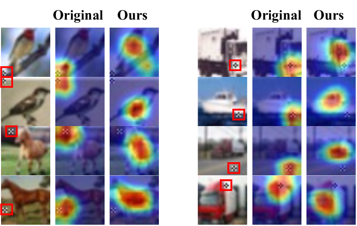
Figure S7: Visualization of attention heatmaps generated by the original backdoored model (Original) and the model repaired using our method (Ours). The red boxes highlight the backdoor triggers in the original images. The original backdoored model focuses primarily on the trigger regions, while our method successfully shifts attention to classification-relevant areas, demonstrating effective backdoor defense.

K.3 Semantic Segmentation with Unlearning

Implementation Details. In this part, we explore the application of machine unlearning in the downstream task of semantic segmentation. Semantic segmentation aims to classify every pixel in an image, thereby generating a segmentation map. We use the DeepLab v3+ model [9] and the PASCAL VOC dataset [15] to conduct segmentation experiments.

Similar to unlearning in classification, we first train a segmentation model from scratch, and then unlearn an entire class from it. During the pretraining phase, we employ SGD optimization with a learning rate of 0.007, weight decay of 5e-4, and train for 50 epochs. Then we perform unlearning over 10 epochs.

To evaluate the methods’ unlearning and remaining performance, we measure the Intersection over Union (IoU) on the test set. The IoU quantifies the overlap between the model’s predicted segmentation map and the ground truth; a higher IoU indicates better segmentation performance. We compute the IoU for the forgotten class, denoted as $\textbf{IoU}_{\textbf{ft}}$, and the average IoU for the remaining classes, denoted as $\textbf{IoU}_{\textbf{rt}}$. In machine unlearning, a lower $\textrm{IoU}_{\textrm{ft}}$ indicates more effective unlearning, while a higher $\textrm{IoU}_{\textrm{rt}}$ suggests that the knowledge on remaining classes is less affected.

Qualitative and Quantitative Results. In terms of quantitative results, as shown in Tab. S14, our method achieves 0% IoU for the forgotten class and 68.93% IoU for the remaining classes, delivering performance closest to that of the retrain model. Other methods, while failing to effectively unlearn, exhibit a significant performance drop of over 25% in $\textrm{IoU}_{\textrm{rt}}$, indicating their inability to achieve effective unlearning or sufficient preservation of the remaining knowledge.

We further present the visualization of segmented results before and after unlearning in Fig. S8. The left three columns show segmentation results for images containing only the car class. While the original model correctly identifies and outlines the car, the unlearned model has “forgotten” and no longer detects it. The right three columns depict images with car and other objects, demonstrating that the target class is successfully forgotten, and the segmentation of people remains preserved.

Table S14: Performance comparison of different unlearning methods on the semantic segmentation task.

Metric	Retrain Model	Negative Gradient	Random Label	Ours
$\textrm{IoU}_{\textrm{ft}}$ $\downarrow$	0	10.26	22.26	0
$\textrm{IoU}_{\textrm{rt}}$ $\uparrow$	71.55	42.26	45.06	68.93

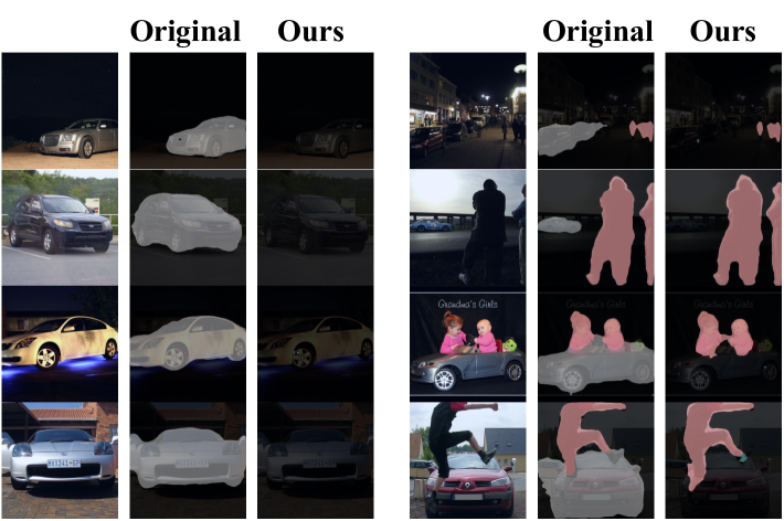
Figure S8: Visualization of machine unlearning in the semantic segmentation task, including segmentation results generated by the original model (Original) and the unlearned model with our method (Ours).

References

- Acquisti [2010] Alessandro Acquisti. The economics of personal data and the economics of privacy. Economics, 2010.
- Baumhauer et al. [2022] Thomas Baumhauer, Pascal Schöttle, and Matthias Zeppelzauer. Machine unlearning: Linear filtration for logit-based classifiers. Machine Learning, 2022.
- Bourtoule et al. [2021] Lucas Bourtoule, Varun Chandrasekaran, Christopher A Choquette-Choo, Hengrui Jia, Adelin Travers, Baiwu Zhang, David Lie, and Nicolas Papernot. Machine unlearning. In S&P, 2021.
- Brophy and Lowd [2021] Jonathan Brophy and Daniel Lowd. Machine unlearning for random forests. In ICML, 2021.
- Cao et al. [2018] Qiong Cao, Li Shen, Weidi Xie, Omkar M Parkhi, and Andrew Zisserman. Vggface2: A dataset for recognising faces across pose and age. In FG, 2018.
- Cao et al. [2024] Shuo Cao, Yihao Liu, Wenlong Zhang, Yu Qiao, and Chao Dong. Grids: Grouped multiple-degradation restoration with image degradation similarity. In ECCV, 2024.
- Cao and Yang [2015] Yinzhi Cao and Junfeng Yang. Towards making systems forget with machine unlearning. In S&P, 2015.
- Cha et al. [2024] Sungmin Cha, Sungjun Cho, Dasol Hwang, Honglak Lee, Taesup Moon, and Moontae Lee. Learning to unlearn: Instance-wise unlearning for pre-trained classifiers. In AAAI, 2024.
- Chen et al. [2018] Liang-Chieh Chen, Yukun Zhu, George Papandreou, Florian Schroff, and Hartwig Adam. Encoder-decoder with atrous separable convolution for semantic image segmentation. In ECCV, 2018.
- Chen et al. [2023] Min Chen, Weizhuo Gao, Gaoyang Liu, Kai Peng, and Chen Wang. Boundary unlearning: Rapid forgetting of deep networks via shifting the decision boundary. In CVPR, 2023.
- Chen et al. [2019] Yuantao Chen, Jie Xiong, Weihong Xu, and Jingwen Zuo. A novel online incremental and decremental learning algorithm based on variable support vector machine. Cluster Computing, 2019.
- Chundawat et al. [2023] Vikram S Chundawat, Ayush K Tarun, Murari Mandal, and Mohan Kankanhalli. Can bad teaching induce forgetting? unlearning in deep networks using an incompetent teacher. In AAAI, 2023.
- Crawford and Paglen [2021] Kate Crawford and Trevor Paglen. Excavating AI: the politics of images in machine learning training sets. AI Soc., 2021.
- Dosovitskiy [2020] Alexey Dosovitskiy. An image is worth 16x16 words: Transformers for image recognition at scale. arXiv preprint arXiv:2010.11929, 2020.
- Everingham et al. [2010] Mark Everingham, Luc Van Gool, Christopher K. I. Williams, John M. Winn, and Andrew Zisserman. The pascal visual object classes (VOC) challenge. IJCV, 2010.
- Fan et al. [2023] Chongyu Fan, Jiancheng Liu, Yihua Zhang, Eric Wong, Dennis Wei, and Sijia Liu. Salun: Empowering machine unlearning via gradient-based weight saliency in both image classification and generation. arXiv preprint arXiv:2310.12508, 2023.
- Foster et al. [2024] Jack Foster, Stefan Schoepf, and Alexandra Brintrup. Fast machine unlearning without retraining through selective synaptic dampening. In AAAI, 2024.
- Gandikota et al. [2023a] Rohit Gandikota, Joanna Materzynska, Jaden Fiotto-Kaufman, and David Bau. Erasing concepts from diffusion models. In ICCV, 2023a.
- Gandikota et al. [2023b] Rohit Gandikota, Joanna Materzynska, Jaden Fiotto-Kaufman, and David Bau. Erasing concepts from diffusion models. In CVPR, 2023b.
- Ginart et al. [2019] Antonio Ginart, Melody Guan, Gregory Valiant, and James Y Zou. Making ai forget you: Data deletion in machine learning. In NeurIPS, 2019.
- Golatkar et al. [2020] Aditya Golatkar, Alessandro Achille, and Stefano Soatto. Eternal sunshine of the spotless net: Selective forgetting in deep networks. In CVPR, 2020.
- Gou et al. [2021] Jianping Gou, Baosheng Yu, Stephen J Maybank, and Dacheng Tao. Knowledge distillation: A survey. IJCV, 2021.
- Graves et al. [2021] Laura Graves, Vineel Nagisetty, and Vijay Ganesh. Amnesiac machine learning. In AAAI, 2021.
- Gu et al. [2017] Tianyu Gu, Brendan Dolan-Gavitt, and Siddharth Garg. Badnets: Identifying vulnerabilities in the machine learning model supply chain. CoRR, 2017.
- Hanzlik et al. [2021] Lucjan Hanzlik, Yang Zhang, Kathrin Grosse, Ahmed Salem, Maximilian Augustin, Michael Backes, and Mario Fritz. Mlcapsule: Guarded offline deployment of machine learning as a service. In CVPR, 2021.
- He et al. [2016] Kaiming He, Xiangyu Zhang, Shaoqing Ren, and Jian Sun. Deep residual learning for image recognition. In CVPR, 2016.
- Hinton [2015] Geoffrey Hinton. Distilling the knowledge in a neural network. arXiv preprint arXiv:1503.02531, 2015.
- Izzo et al. [2021] Zachary Izzo, Mary Anne Smart, Kamalika Chaudhuri, and James Zou. Approximate data deletion from machine learning models. In AISTATS, 2021.
- Krizhevsky et al. [2009] Alex Krizhevsky, Geoffrey Hinton, et al. Learning multiple layers of features from tiny images. Technical report, 2009.
- Kurmanji et al. [2024] Meghdad Kurmanji, Peter Triantafillou, Jamie Hayes, and Eleni Triantafillou. Towards unbounded machine unlearning. In NeurIPS, 2024.
- Le and Yang [2015] Ya Le and Xuan Yang. Tiny imagenet visual recognition challenge. CS 231N, 2015.
- Li et al. [2024] Na Li, Chunyi Zhou, Yansong Gao, Hui Chen, Anmin Fu, Zhi Zhang, and Yu Shui. Machine unlearning: Taxonomy, metrics, applications, challenges, and prospects. arXiv preprint arXiv:2403.08254, 2024.
- Li et al. [2021] Yige Li, Xixiang Lyu, Nodens Koren, Lingjuan Lyu, Bo Li, and Xingjun Ma. Neural attention distillation: Erasing backdoor triggers from deep neural networks. In ICLR, 2021.
- Liu et al. [2018] Kang Liu, Brendan Dolan-Gavitt, and Siddharth Garg. Fine-pruning: Defending against backdooring attacks on deep neural networks. In RAID, 2018.
- Liu et al. [2022] Yang Liu, Mingyuan Fan, Cen Chen, Ximeng Liu, Zhuo Ma, Li Wang, and Jianfeng Ma. Backdoor defense with machine unlearning. In INFOCOM, 2022.
- Liu et al. [2021] Ze Liu, Yutong Lin, Yue Cao, Han Hu, Yixuan Wei, Zheng Zhang, Stephen Lin, and Baining Guo. Swin transformer: Hierarchical vision transformer using shifted windows. In ICCV, 2021.
- Liu et al. [2023] Zuhao Liu, Xiao-Ming Wu, Dian Zheng, Kun-Yu Lin, and Wei-Shi Zheng. Generating anomalies for video anomaly detection with prompt-based feature mapping. In CVPR, 2023.
- Lv et al. [2024] Zhen Lv, Yangqi Long, Congzhentao Huang, Cao Li, Chengfei Lv, Hao Ren, and Dian Zheng. Spatialdreamer: Self-supervised stereo video synthesis from monocular input. arXiv preprint arXiv:2411.11934, 2024.
- Mahadevan and Mathioudakis [2021] Ananth Mahadevan and Michael Mathioudakis. Certifiable machine unlearning for linear models. arXiv preprint arXiv:2106.15093, 2021.
- Mo et al. [2024] Qijie Mo, Yipeng Gao, Shenghao Fu, Junkai Yan, Ancong Wu, and Wei-Shi Zheng. Bridge past and future: Overcoming information asymmetry in incremental object detection. In ECCV, 2024.
- Nguyen et al. [2022] Thanh Tam Nguyen, Thanh Trung Huynh, Phi Le Nguyen, Alan Wee-Chung Liew, Hongzhi Yin, and Quoc Viet Hung Nguyen. A survey of machine unlearning. arXiv preprint arXiv:2209.02299, 2022.
- Oesterling et al. [2024] Alex Oesterling, Jiaqi Ma, Flavio Calmon, and Himabindu Lakkaraju. Fair machine unlearning: Data removal while mitigating disparities. In AISTATS, 2024.
- Qiao et al. [2019] Ximing Qiao, Yukun Yang, and Hai Li. Defending neural backdoors via generative distribution modeling. In NeurIPS, 2019.
- Romero et al. [2014] Adriana Romero, Nicolas Ballas, Samira Ebrahimi Kahou, Antoine Chassang, Carlo Gatta, and Yoshua Bengio. Fitnets: Hints for thin deep nets. arXiv preprint arXiv:1412.6550, 2014.
- Salimans and Ho [2022] Tim Salimans and Jonathan Ho. Progressive distillation for fast sampling of diffusion models. arXiv preprint arXiv:2202.00512, 2022.
- Sanh [2019] V Sanh. Distilbert, a distilled version of bert: smaller, faster, cheaper and lighter. arXiv preprint arXiv:1910.01108, 2019.
- Schramowski et al. [2023] Patrick Schramowski, Manuel Brack, Björn Deiseroth, and Kristian Kersting. Safe latent diffusion: Mitigating inappropriate degeneration in diffusion models. In CVPR, 2023.
- Schuhmann et al. [2022] Christoph Schuhmann, Romain Beaumont, Richard Vencu, Cade Gordon, Ross Wightman, Mehdi Cherti, Theo Coombes, Aarush Katta, Clayton Mullis, Mitchell Wortsman, et al. Laion-5b: An open large-scale dataset for training next generation image-text models. In NeurIPS, 2022.
- Selvaraju et al. [2017] Ramprasaath R Selvaraju, Michael Cogswell, Abhishek Das, Ramakrishna Vedantam, Devi Parikh, and Dhruv Batra. Grad-cam: Visual explanations from deep networks via gradient-based localization. In ICCV, 2017.
- Shan et al. [2023] Shawn Shan, Jenna Cryan, Emily Wenger, Haitao Zheng, Rana Hanocka, and Ben Y Zhao. Glaze: Protecting artists from style mimicry by text-to-image models. arXiv preprint arXiv:2302.04222, 2023.
- Shen et al. [2024] Shaofei Shen, Chenhao Zhang, Yawen Zhao, Alina Bialkowski, Weitong Tony Chen, and Miao Xu. Label-agnostic forgetting: A supervision-free unlearning in deep models. arXiv preprint arXiv:2404.00506, 2024.
- Shokri et al. [2017] Reza Shokri, Marco Stronati, Congzheng Song, and Vitaly Shmatikov. Membership inference attacks against machine learning models. In S&P, 2017.
- Simonyan and Zisserman [2014] Karen Simonyan and Andrew Zisserman. Very deep convolutional networks for large-scale image recognition. arXiv preprint arXiv:1409.1556, 2014.
- Song and Mittal [2021] Liwei Song and Prateek Mittal. Systematic evaluation of privacy risks of machine learning models. In USENIX, 2021.
- Tang et al. [2024] Yu-Ming Tang, Yi-Xing Peng, Jingke Meng, and Wei-Shi Zheng. Rethinking few-shot class-incremental learning: Learning from yourself. In ECCV, 2024.
- Tarun et al. [2023] Ayush K Tarun, Vikram S Chundawat, Murari Mandal, and Mohan Kankanhalli. Fast yet effective machine unlearning. TNNLS, 2023.
- Thudi et al. [2022a] Anvith Thudi, Gabriel Deza, Varun Chandrasekaran, and Nicolas Papernot. Unrolling sgd: Understanding factors influencing machine unlearning. In EuroS&P, 2022a.
- Thudi et al. [2022b] Anvith Thudi, Hengrui Jia, Ilia Shumailov, and Nicolas Papernot. On the necessity of auditable algorithmic definitions for machine unlearning. In USENIX Security, 2022b.
- Van der Maaten and Hinton [2008] Laurens Van der Maaten and Geoffrey Hinton. Visualizing data using t-sne. JMLR, 2008.
- Voigt and Von dem Bussche [2017] Paul Voigt and Axel Von dem Bussche. The eu general data protection regulation (gdpr). A Practical Guide, 1st Ed., Cham: Springer International Publishing, 2017.
- Wang et al. [2019] Tao Wang, Li Yuan, Xiaopeng Zhang, and Jiashi Feng. Distilling object detectors with fine-grained feature imitation. In CVPR, 2019.
- Weng et al. [2022] Qizhen Weng, Wencong Xiao, Yinghao Yu, Wei Wang, Cheng Wang, Jian He, Yong Li, Liping Zhang, Wei Lin, and Yu Ding. Mlaas in the wild: Workload analysis and scheduling in large-scale heterogeneous gpu clusters. In NSDI, 2022.
- Wu et al. [2023] Xiao-Ming Wu, Dian Zheng, Zuhao Liu, and Wei-Shi Zheng. Estimator meets equilibrium perspective: A rectified straight through estimator for binary neural networks training. In ICCV, 2023.
- Wu et al. [2024] Xiao-Ming Wu, Jia-Feng Cai, Jian-Jian Jiang, Dian Zheng, Yi-Lin Wei, and Wei-Shi Zheng. An economic framework for 6-dof grasp detection. In ECCV, 2024.
- Wu et al. [2020] Yinjun Wu, Edgar Dobriban, and Susan Davidson. Deltagrad: Rapid retraining of machine learning models. In ICML, 2020.
- Xu et al. [2024] Guo-Hao Xu, Yi-Lin Wei, Dian Zheng, Xiao-Ming Wu, and Wei-Shi Zheng. Dexterous grasp transformer. In CVPR, 2024.
- Xu et al. [2023] Heng Xu, Tianqing Zhu, Lefeng Zhang, Wanlei Zhou, and Philip S. Yu. Machine unlearning: A survey. ACM Comput. Surv., 2023.
- Zhao et al. [2022] Borui Zhao, Quan Cui, Renjie Song, Yiyu Qiu, and Jiajun Liang. Decoupled knowledge distillation. In CVPR, 2022.
- Zhao et al. [2024] Hongbo Zhao, Bolin Ni, Junsong Fan, Yuxi Wang, Yuntao Chen, Gaofeng Meng, and Zhaoxiang Zhang. Continual forgetting for pre-trained vision models. In CVPR, 2024.
- Zheng et al. [2024] Dian Zheng, Xiao-Ming Wu, Shuzhou Yang, Jian Zhang, Jian-Fang Hu, and Wei-Shi Zheng. Selective hourglass mapping for universal image restoration based on diffusion model. In CVPR, 2024.
- Zheng et al. [2025a] Dian Zheng, Ziqi Huang, Hongbo Liu, Kai Zou, Yinan He, Fan Zhang, Yuanhan Zhang, Jingwen He, Wei-Shi Zheng, Yu Qiao, et al. Vbench-2.0: Advancing video generation benchmark suite for intrinsic faithfulness. arXiv preprint arXiv:2503.21755, 2025a.
- Zheng et al. [2025b] Dian Zheng, Xiao-Ming Wu, Zuhao Liu, Jingke Meng, and Wei-shi Zheng. Diffuvolume: Diffusion model for volume based stereo matching. IJCV, 2025b.