On an approach to canonicalizing elliptic Feynman integrals

Abstract

We present a systematic method for the construction of canonical bases for univariate elliptic Feynman integrals with multiple kinematic scales, which frequently arise in phenomenologically relevant scattering processes. The construction is performed in the Legendre normal form of elliptic curves, where the geometric propoerties of the curves are simple and explicit and further kinemtic singularities are present as marked points. The canonical bases are constructed using Abelian differentials of three kinds with a universal linear transformation. The bases constructed in the normal form can be mapped to generic integral families via an appropriate Möbius transformation. As a demonstration, we discuss the application of our method to several concrete examples, where we show that the $\varepsilon$-factorization of sub-sector dependence can also be simply done. Our method can be readily applied to more complicated integral families straightforwardly.

1 Introduction

With the construction of the High Luminosity-Large Hadron Collider (HL-LHC) Cepeda:2019klc and prospective high-energy colliders such as the Circular Electron Positron Collider (CEPC) CEPCStudyGroup:2018ghi and the Future Circular Collider (FCC) FCC:2018byv ; FCC:2018evy ; FCC:2018vvp , which promise greater luminosity and energy, we are on the verge of exploring fundamental natural phenomena with unprecedented precision. These experimental advancements provide a robust testing ground for the Standard Model (SM), allowing physicists to rigorously validate its predictions, identify potential limitations, and perhaps even discover signs of new physics.

To fully exploit the anticipated wealth of experimental data, highly accurate theoretical predictions are essential. Such predictions are grounded in quantum field theory (QFT) and are typically obtained through perturbative expansion, which necessitates calculating a variety of Feynman integrals. Understanding the mathematical structure of these integrals is crucial to their computation (see Weinzierl:2022eaz ; Abreu:2022mfk ; Badger:2023eqz for recent reviews). Each integral family spans a finite-dimensional linear space, with its basis integrals known as master integrals (MIs). Any integral within the family can be expressed as a linear combination of MIs, often through integration-by-parts (IBP) identities Tkachov:1981wb ; Chetyrkin:1981qh , which are systematically solved using the Laporta algorithm Laporta:2000dsw . Several public software packages, such as Reduze Studerus:2009ye ; vonManteuffel:2012np , LiteRed Lee:2012cn ; Lee:2013mka , FIRE Smirnov:2019qkx ; Smirnov:2023yhb , and Kira Maierhofer:2017gsa ; Klappert:2020nbg , implement this algorithm. There are also efforts to work in a smaller linear equations system, such as NeatIBP Wu:2023upw ; Wu:2025aeg based on syzygy method and Blade Guan:2024byi based on the method of block-triangular form. Recently, Feynman integrals have been reinterpreted within twisted (co-)homology as twisted periods Aomoto:2011ggg , enabling reduction via intersection numbers Mastrolia:2018uzb ; Frellesvig:2019uqt rather than traditional IBP equations.

The differential equations method Kotikov:1990kg ; Kotikov:1991pm ; Remiddi:1997ny ; Gehrmann:1999as , and specifically the canonical differential equations approach Henn:2013pwa , represents the state-of-the-art method for calculating MIs analytically. This approach leverages an $\varepsilon$-factorized form, allowing MIs to be expressed as Laurent expansions in the dimensional regulator $\varepsilon$, with Chen’s iterated integrals Chen:1977oja as coefficients. The simplest iterated integrals found in Feynman integrals are multiple polylogarithms (MPLs) Goncharov:1998kja ; Goncharov:2001iea ; Vollinga:2004sn , which are iterated integrals over the genus-$0$ Riemann sphere with marked points, or say over moduli space ${\cal M}_{0,n}$ Bogner:2014mha . For MPL integral families, canonical differential equations can be achieved through rational and algebraic transformations alone, and several tools are available to assist in identifying such transformations Gituliar:2017vzm ; Prausa:2017ltv ; Meyer:2017joq ; Lee:2020zfb ; Dlapa:2020cwj . An alternative approach constructs canonical bases through ${\rm d}\log$-forms Henn:2020lye ; Chen:2020uyk ; Chen:2022lzr . MPLs exhibit properties that facilitate algorithmic extraction of critical information, aiding in the construction of canonical bases and enriching our understanding of their mathematical structure.

However, as the complexity of the problem increases with additional loops and mass scales, the MPL functions space becomes insufficient to accommodate all integrals within an integral family (see, e.g., Bourjaily:2022bwx for a recent review). In these cases, elliptic integrals—the next class of iterated integrals—emerge, first noted in the context of the two-loop electron self-energy in QED Sabry:1962rge . Fully analytic results for this case were obtained only half a century later Honemann:2018mrb , and additional significant calculations involving more scales or higher loops are found in works such as Bogner:2019lfa ; Giroux:2024yxu ; Pogel:2022yat ; Pogel:2022ken ; Pogel:2022vat . Three-loop corrections have also been computed in recent studies Duhr:2024bzt . Elliptic Feynman integrals are iterated integrals over a genus-$1$ Riemann surface, or say torus, with marked points, equivalently, over moduli space ${\cal M}_{1,n}$ Weinzierl:2020kyq . Unlike MPLs, which are defined on the Riemann sphere with a unique shape, the genus-$1$ Riemann surface underlying elliptic Feynman integrals varies and can be parameterized by a modular variable, $\tau$. To express the $\varepsilon$-expansion of elliptic Feynman integrals, we need both the elliptic multiple polylogarithms (eMPLs) Levin:2007tto ; Brown:2011wfj ; Broedel:2017kkb and iterated integrals of modular forms or Eisenstein series Adams:2017ejb ; Broedel:2018iwv ; Duhr:2019rrs ; Weinzierl:2020kyq . It’s well-known that the underlying geometry for an integral can be made explicit with the analysis of leading singularities Cachazo:2008vp ; Arkani-Hamed:2010pyv . Specially, the underlying elliptic curve of an elliptic sector can be identified in (loop-by-loop) Baikov representations Baikov:1996rk ; Baikov:1996iu ; Frellesvig:2017aai ; Harley:2017qut through the maximal cut Frellesvig:2017aai ; Harley:2017qut ; Primo:2016ebd ; Bosma:2017ens ; Primo:2017ipr . Implementations for (loop-by-loop) Baikov representations are offered by Frellesvig:2017aai ; Jiang:2023qnl ; Jiang:2024eaj ; Frellesvig:2024ymq ; Correia:2025yao . Alternatively, we can study the elliptic curve by analyzing the periods of the elliptic curve through solutions to a second-order irreducible Picard-Fuchs operator Adams:2017tga ; Adams:2018bsn ; Adams:2018kez .

Due to the success of the method of canonical differential equations in solving the MPL integral families, there have been substantial efforts to extend the method to the elliptic cases appearing in various scattering processes Muller:2022gec ; Jiang:2023jmk ; Gorges:2023zgv ; Delto:2023kqv ; Wang:2024ilc ; Forner:2024ojj ; Schwanemann:2024kbg ; Marzucca:2025eak ; Becchetti:2025rrz ; Becchetti:2025oyb . In such cases, there are subtleties in the precise definition of “canonical” Broedel:2018iwv ; Broedel:2018qkq ; Broedel:2019hyg ; Dlapa:2022wdu ; Frellesvig:2023iwr ; Duhr:2024uid ; Duhr:2025lbz , but one may at least attempt to obtain an $\varepsilon$-factorized system of differential equations which still offers simplification in the calculations. There are now several methods for deriving $\varepsilon$-factorized bases for elliptic cases vonManteuffel:2017hms ; Adams:2018bsn ; Frellesvig:2021hkr ; Pogel:2022vat ; Giroux:2022wav ; Dlapa:2022wdu ; Gorges:2023zgv , and some of them can even be extended to more complex geometries, such as Calabi-Yau varieties. At the moment, finding $\varepsilon$-factorized bases still requires non-trivial case-by-case analyses, especially when there are multiple kinematic marked points Bogner:2019lfa ; Gorges:2023zgv ; Delto:2023kqv ; Schwanemann:2024kbg ; Becchetti:2025rrz . This raises the natural question of whether it is possible to directly construct the $\varepsilon$-factorized basis for an elliptic Feynman integral family analogous to the approach for MPLs in Chen:2020uyk ; Chen:2022lzr .

In this paper, we introduce a novel method to systematize the construction of canonical bases for univariate elliptic Feynman integrals under the maximal cut. We use the term “canonical” here since it meets most of the important properties advocated by the literature Dlapa:2022wdu ; Frellesvig:2023iwr ; Duhr:2024uid . Our method utilizes Legendre normal form of elliptic curves, where the geometric properties of the curves are simple and explicit. We then construct the pre-canonical basis using Abelian differentials of three kinds, accounting for an arbitrary number of kinematic marked points. The differential equations of the pre-canonical basis can be straightforwardly converted to the $\varepsilon$-factorized form with a universal transformation. Such a construction can be applied to arbitrary elliptic curves with appropriate Möbius transformations which transform the curves to the Legendre normal form.

To demonstrate our construction, we apply the method to several concrete examples: fully massive sunrise and non-planar double box diagrams, each with two kinds of mass configurations. We show that it is rather straightforward to derive an $\varepsilon$-factorized system of differential equations within the top sectors. To obtain a canonical basis for the entire integral family, we still need to address the non-$\varepsilon$-factorized dependence on the sub-sectors. Ideally speaking, one would imagine that it is possible to construct the full integrand without any cut, combining the top-sector construction in this work and the ${\rm d}\log$-form construction in Chen:2020uyk ; Chen:2022lzr . In this work, we simply convert the differential equations to the $\varepsilon$-factorized form through linear transformation. We show in the examples that the nice properties of our basis helps a lot in this process.

This paper is organized as follows. In Sec. 2, We present the construction of the canonical basis under maximal cut, which involves the construction in the Legendre normal form and the transformation to an elliptic curve defined by an arbitrary degree-4 polynomial. We demonstrate the procedure with several examples in Sec. 3, where the transformation to a canonical basis for the full family without cut is discussed. The summary and outlook are provided in Sec. 4. There are a few appendices at the end of the paper. A different strategy vonManteuffel:2017hms ; Frellesvig:2021hkr for deriving an $\varepsilon$-factorized basis is presented in App. A. The construction using the Jacobi normal form of elliptic curves is discussed in App. B. Some lengthy expressions relevant for the examples in Sec. 3 are collected in App. C. Special relations between elliptic integrals are compiled in App. D.

2 Canonical basis under the maximal cut

In this section, we first briefly review some basics for elliptic Feynman integrals. Then, we present a general approach to construct a pre-canonical basis in elliptic sectors, which can be easily converted to a canonical basis under the maximal cut. We will first perform the construction in terms of the Legendre form $P_{L}(x)$ of the elliptic curve and then transform to the quartic family $P_{4}(z)$, which is commonly used in the Baikov representation with a suitable Möbius transformation. Finally, we construct the transformation to the canonical basis, which can be used directly in both the Legendre family and the quartic family.

2.1 Basics for elliptic Feynman integrals

Integral family

An $L$-loop Feynman integral family with $E+1$ external legs is defined as

$$I_{\nu_{1}\cdots\nu_{N}}=e^{L\varepsilon\gamma_{E}}\left(\mu^{2}\right)^{\nu-Ld/2}\int\,\bigg{[}\,\prod_{j=1}^{L}\frac{{\rm d}^{d}k_{j}}{i\pi^{d/2}}\,\bigg{]}\frac{1}{D_{1}^{\nu_{1}}\cdots D_{N}^{\nu_{N}}}\,,$$ (1)

with $N=L(L+1)/2+LE$, $d=d_{0}-2\varepsilon$ ($d_{0}\in 2\mathbb{Z}^{+}$) and $\nu=\sum_{i=1}^{N}\nu_{i}$. A topology in the family is specified by the set of $D_{i}$ with the corresponding $\nu_{i}$ positive, and the rest of the propagators are irreducible scalar products (ISPs). Unless otherwise stated, we will consider integral families in $d=4-2\varepsilon$.

Elliptic curve

To identify the elliptic curve involved in an integral family, we resort to the maximal cut of the elliptic sector integrals in the (loop-by-loop) Baikov representation. Then the integral family under the cut can be expressed as

$$I=\int_{\cal C}u\,\varphi\,,$$ (2)

where the multi-valued function $u$ (the twist in the language of twisted cohomology) is

$$u=u(z)=\big{(}P_{4}\left(z\right)\big{)}^{-1/2}\prod_{i=1}^{n}\left(z-c_{i}\right)^{-\beta_{i}\varepsilon}\,,$$ (3)

where the branch points $c_{i}$’s are distinct and the corresponding $\beta_{i}$’s are integers. The single-valued differential $1$-form $\varphi=\varphi(z)$ may have poles at some of the branch points $c_{i}$’s. Note that there is an implicit branch point at infinity, which will be denoted as $c_{n+1}\equiv c_{\infty}\equiv\infty$. The elliptic curve is specified by the polynomial equation

$$w^{2}=P_{4}(z)\equiv(z-c_{1})(z-c_{2})(z-c_{3})(z-c_{4})\,,$$ (4)

which is only related to the four branch points $c_{1},c_{2},c_{3}$ and $c_{4}$.

The elliptic curve (4) can be represented in different ways, related by Möbius transformations $(z,w)\mapsto(x,y)$. The shape of the elliptic curve is characterized by the modular lambda $\lambda$,

$$\lambda=\frac{c_{14}c_{23}}{c_{13}c_{24}}\,,\quad(c_{ij}\equiv c_{i}-c_{j})\,.$$ (5)

The Legendre normal form of the elliptic curve is given by

$$y^{2}=P_{L}(x)\equiv x(x-\lambda)(x-1)\,,$$ (6)

with four branch points $0,\lambda,1$ and $\infty$. These four points are related to the previous four branch points, $c_{1}-c_{4}$, of the multi-valued function $w=\sqrt{P_{4}(z)}$ by a Möbius transformation. We will mainly use this form in the construction of the pre-canonical master integrals. In App. B, we will discuss the usage of a different form.

Elliptic integrals

We consider elliptic integrals of the form

$$\int\frac{R(x)\,{\rm d}x}{\sqrt{P_{L}(x)}}\,,$$ (7)

where $R(x)$ is a rational function. They can be converted to combinations of (3 kinds of) standard elliptic integrals by the variable change $x=\lambda t^{2}$:

$$\frac{{\rm d}x}{\sqrt{P_{L}(x)}}=\frac{2\,{\rm d}t}{\sqrt{(1-t^{2})(1-\lambda t^{2})}}\,.$$ (8)

The incomplete elliptic integral of the first kind is defined as

$$F(\theta,\lambda)=\int\limits_{0}^{\sin\theta}\frac{{\rm d}t}{\sqrt{(1-t^{2})(1-\lambda t^{2})}}=\frac{1}{2}\int\limits_{0}^{\lambda\sin^{2}\theta}\frac{{\rm d}x}{\sqrt{P_{L}(x)}}\,,$$ (9)

where the differential is holomorphic. The second kind is defined as

$$E(\theta,\lambda)=\int\limits_{0}^{\sin\theta}\frac{(1-\lambda t^{2}){\rm d}t}{\sqrt{(1-t^{2})(1-\lambda t^{2})}}=\frac{1}{2}\int\limits_{0}^{\lambda\sin^{2}\theta}\frac{(1-x){\rm d}x}{\sqrt{P_{L}(x)}}\,,$$ (10)

where the differential has a double pole at infinity with a vanishing residue. The third kind is defined as

$$\Pi(n,\theta,\lambda)=\int\limits_{0}^{\sin\theta}\frac{1}{1-n\,t^{2}}\,\frac{{\rm d}t}{\sqrt{(1-t^{2})(1-\lambda t^{2})}}=\frac{1}{2}\int\limits_{0}^{\lambda\sin^{2}\theta}\frac{1}{1-n\,x/\lambda}\,\frac{{\rm d}x}{\sqrt{P_{L}(x)}}\,,$$ (11)

with the parameter $n$ characterizing the simple poles of the differential at $t=\pm 1/{\sqrt{n}}$ or $x=\lambda/n$. The three kinds of complete elliptic integrals are given by the incomplete ones with $\theta=\pi/2$. They’re

$$K(\lambda)=F\left(\frac{\pi}{2},\lambda\right),\quad E(\lambda)=E\left(\frac{\pi}{2},\lambda\right),\quad\Pi(n,\lambda)=\Pi\left(n,\frac{\pi}{2},\lambda\right)\,,$$ (12)

respectively.

2.2 The construction of the pre-canonical basis

We can perform a variable change to transform the polynomial $P_{4}(z)$, which originates from the Baikov representation, to $P_{L}(x)$ as mentioned previously. The details of this transformation will be given later. After the transformation, the four branch points $\{c_{1},c_{2},c_{3},c_{4}\}$ defining the elliptic curve are transformed to $e_{1}=\infty$, $e_{2}=0$, $e_{3}=\lambda$ and $e_{4}=1$. We assume that the branch point $c_{i}$ for $4<i\leq n$ gets transformed to $e_{i}$, and $c_{n+1}=c_{\infty}$ is transformed to $e_{n+1}\equiv e_{\infty}$. We also want to stress that in $P_{L}(x)$, the point at the infinity or, say, $e_{1}$ is a branch point of the curve. However, $e_{\infty}$, which corresponds to the point of infinity in the original $P_{4}(z)$, is different from $e_{1}$ and no longer the point at infinity in the Legendre family. The transformed $u$ function is then given by

$$u_{L}(x)=P_{L}(x)^{-1/2}\prod_{i=2}^{n+1}(x-e_{i})^{-\beta_{i}\varepsilon}\,,$$ (13)

where

$$\beta_{n+1}=-\sum_{i=1}^{n}\beta_{i}\,.$$ (14)

We can then consider integrals of the form

$$I=\int_{\cal C}u_{L}(x)\,\varphi=\int_{\cal C}\widebar{u}_{L}(x)\,\phi=\int_{\cal C}\phi\prod_{i=2}^{n+1}(x-e_{i})^{-\beta_{i}\varepsilon}\,,$$ (15)

where for later convenience we have defined

$$\phi=\frac{\varphi}{\sqrt{P_{L}(x)}}\,,\quad\widebar{u}_{L}(x)=\prod_{i=2}^{n+1}(x-e_{i})^{-\beta_{i}\varepsilon}.$$ (16)

Here $\phi=\phi(x)=\phi\left(z(x)\right)$ for brevity, and we have introduced the reduced twist $\widebar{u}_{L}$. Likewise, we define the reduced twist

$$\widebar{u}(z)=\prod_{i=1}^{n}(z-c_{i})^{-\beta_{i}\varepsilon},$$ (17)

and absorb $P^{-1/2}_{4}(z)$ into the differential 1-form as the above.

We now propose a set of candidates for the pre-canonical basis, motivated by the three kinds of standard elliptic integrals:

$$\phi_{1} =\frac{{\rm d}x}{\sqrt{P_{L}(x)}}=2\,{\rm d}F\left(\sin^{-1}\sqrt{\frac{x}{\lambda}},\lambda\right)\,,$$ (18a)

$$\phi_{i-3} =\frac{1}{x-e_{i}}\frac{\sqrt{P_{L}(e_{i})}}{\sqrt{P_{L}(x)}}{\rm d}x=-\frac{2\sqrt{P_{L}(e_{i})}}{e_{i}}\,{\rm d}\Pi\left(\frac{\lambda}{e_{i}},\sin^{-1}\sqrt{\frac{x}{\lambda}},\lambda\right)\,,$$ (18b)

$$\phi_{n-1} =\frac{x{\rm d}x}{\sqrt{P_{L}(x)}}=2\,{\rm d}F\left(\sin^{-1}\sqrt{\frac{x}{\lambda}},\lambda\right)-2\,{\rm d}E\left(\sin^{-1}\sqrt{\frac{x}{\lambda}},\lambda\right)\,,$$ (18c)

where $i=5,\cdots,n+1$. Note that the number of master integrals is $n-1$. The first and the last candidates involve differentials of the first and second kinds of standard elliptic integrals, while the rest involve the third kind. Plugging these $\phi_{j}$’s into Eq. (15), we get the corresponding master integrals $I_{j}$’s.

We can now derive the differential equations of the master integrals with respect to $\lambda$ and $e_{i}$ for $i=5,\cdots,n+1$. We find that they are in a special linear form:

$${\rm d}\vec{I}=\bm{A}\,\vec{I}=\left({\bm{A}^{(0)}}+\varepsilon{\bm{A}^{(1)}}\right)\vec{I}\,,$$ (19)

where the matrices $\bm{A}^{(0)}$ and ${\bm{A}^{(1)}}$ are independent of $\varepsilon$. To convert the above differential equations to the $\varepsilon$-factorized form, we only need to rotate $\bm{A}^{(0)}$ away by a linear transformation of the master integrals $\vec{I}$. Therefore, the explicit form of $\bm{A}^{(0)}$ is particularly important in this context. The coefficient matrix of $\mathrm{d}\lambda$ in $\bm{A}^{(0)}$ has the form

$$\begin{pmatrix}\frac{1}{2(1-\lambda)}&0&\cdots&0&-\frac{1}{2\lambda(1-\lambda)}\\ -\frac{e_{5}(e_{5}-1)}{2(1-\lambda)\sqrt{P_{L}(e_{5})}}&0&\cdots&0&\frac{e_{5}(e_{5}-1)}{2\lambda\left(1-\lambda\right)\sqrt{P_{L}(e_{5})}}\\ \vdots&\vdots&\ddots&\vdots&\vdots\\ -\frac{e_{n+1}(e_{n+1}-1)}{2(1-\lambda)\sqrt{P_{L}(e_{n+1})}}&0&\cdots&0&\frac{e_{n+1}(e_{n+1}-1)}{2\lambda(1-\lambda)\sqrt{P_{L}(e_{n+1})}}\\ \frac{1}{2(1-\lambda)}&0&\cdots&0&-\frac{1}{2(1-\lambda)}\end{pmatrix},$$ (20)

while the coefficient matrix of $\mathrm{d}e_{i}$ ($i=5,\cdots,n+1$) is

$$\begin{pmatrix}0&0&\cdots&0&0\\ \vdots&\vdots&\ddots&\vdots&\vdots\\ -\frac{e_{i}}{2\sqrt{P_{L}(e_{i})}}&0&\cdots&0&\frac{1}{2\sqrt{P_{L}(e_{i})}}\\ \vdots&\vdots&\ddots&\vdots&\vdots\\ 0&0&\cdots&0&0\end{pmatrix}.$$ (21)

The special linear form as Eq. (19) is an essential step towards deriving the $\varepsilon$-factorized form of the integral family, which will be elaborated in detail in Sec. 2.3 and App. A. In particular, $\bm{A}^{(0)}$ is closely related to the geometry behind the integral family and plays an important role in the later derivation. It is a good place here to put some remarks about it. For this purpose, we take $\varepsilon=0$ in this discussion. With a bit of abuse of notation, we are interested in the following equation:

$${\rm d}\vec{I}^{(0)}={\bm{A}^{(0)}}\vec{I}^{(0)}\,.$$ (22)

Then based on the general structure given by Eq. (20) and (21), we observe that

$$\begin{aligned} {\rm d}\begin{pmatrix}I_{1}^{(0)}\\ I_{n-1}^{(0)}\end{pmatrix}=\begin{pmatrix}\frac{{\rm d}\lambda}{2(1-\lambda)}&-\frac{{\rm d}\lambda}{2\lambda(1-\lambda)}\\ \frac{{\rm d}\lambda}{2(1-\lambda)}&-\frac{{\rm d}\lambda}{2(1-\lambda)}\end{pmatrix}\begin{pmatrix}I_{1}^{(0)}\\ I_{n-1}^{(0)}\end{pmatrix}\end{aligned},$$ (23)

which equivalently defines the elliptic curve while

$${\rm d}I_{i-3}^{(0)}=-\left[\frac{e_{i}(e_{i}-1)}{(1-\lambda)}\frac{{\rm d}\lambda}{2\sqrt{P_{L}(e_{i})}}+\frac{e_{i}{\rm d}e_{i}}{2\sqrt{P_{L}(e_{i})}}\right]I_{1}^{(0)}+\left[\frac{e_{i}(e_{i}-1)}{\lambda(1-\lambda)}\frac{{\rm d}\lambda}{2\sqrt{P_{L}(e_{i})}}+\frac{{\rm d}e_{i}}{2\sqrt{P_{L}(e_{i})}}\right]I_{n-1}^{(0)},$$ (24)

with $5\leq i\leq n+1$, which is related to the marked points information in that curve. Denoting

$$E=E\left(\sin^{-1}\sqrt{\frac{e_{i}}{\lambda}},\lambda\right),\quad F=F\left(\sin^{-1}\sqrt{\frac{e_{i}}{\lambda}},\lambda\right)$$ (25)

for brevity, then the right-hand side of the above can be written as a closed form:

$${\rm d}I_{i-3}^{(0)} =-\left[{\rm d}(F-E)-E\frac{{\rm d}\lambda}{2(1-\lambda)}\right]I_{1}^{(0)}+\left[{\rm d}F+\left(\frac{F}{2\lambda}-\frac{E}{2\lambda(1-\lambda)}\right){\rm d}\lambda\right]I_{n-1}^{(0)}$$ (26)

$$=-{\rm d}\left[(F-E)I_{1}^{(0)}-FI_{n-1}^{(0)}\right],$$

where the second equality in the above follows with the help of the elliptic information (23). This property motivates us to refine the master integrals $I_{i-3}$ for $5\leq i\leq n+1$, which are directly related to the marked points as

$$I_{i-3}\to I_{i-3}+(F-E)I_{1}-FI_{n-1}.$$ (27)

Then, their differential equations will be automatically $\varepsilon$-factorized.

2.3 The transformation to canonical form

Before we move to the explicit construction of a canonical basis, we would like to give short comments on the relationships between canonical bases and $\varepsilon$-factorized bases. $\varepsilon$-factorization is only one property for a canonical basis, and it cannot uniquely fix the basis, even up to a constant transformation. Such phenomena can stem in polylogarithmic cases as well, if we only ask for $\varepsilon$-factorization. To be more precise, the transformation to an $\varepsilon$-factorized basis can involve transcendental functions like logarithmic functions, while no such functions and only rational or algebraic functions are needed for the transformation to a canonical basis. This fact indicates that there should be some bases more “canonical” than others and it is natural to expect they would degenerate to canonical bases where the elliptic curves degenerate to Riemann spheres Frellesvig:2023iwr .

Our strategy to transform the pre-canonical basis to a canonical one is similar to that of Pogel:2022vat . We note that the method in Gorges:2023zgv leads to equivalent results. The essence of the strategy is to construct the canonical basis with ansatz inspired by the Picard-Fuchs operator for the integral of the first kind, $I_{1}$. In order to apply the method, we first introduce the periods of $\phi_{1}$, which serve as the solutions to the corresponding Picard-Fuchs equations. The periods are the pairings between the differential forms and the integration contours, i.e.,

$$\varpi_{0}(\lambda)\equiv\frac{2}{\pi}\int_{0}^{\lambda}\frac{{\rm d}x}{\sqrt{P_{L}(x)}}=\frac{4}{\pi}K(\lambda)\,,\quad\varpi_{1}(\lambda)\equiv\frac{2i}{\pi}\int_{\lambda}^{1}\frac{{\rm d}x}{\sqrt{P_{L}(x)}}=\frac{4}{\pi}K(1-\lambda)\,,$$ (28)

where $\varpi_{0}(\lambda)$ and $\varpi_{1}(\lambda)$ are holomorphic around degenerate points $\lambda=0$ and $\lambda=1$, respectively. The $1/\pi$ factors are introduced to make the periods of uniform transcendental weight-$0$ around degenerate points, while the $i$ factor in the second period is to make the periods real. The modular $\tau$ is defined as

$$\tau\equiv\frac{i\varpi_{1}(\lambda)}{\varpi_{0}(\lambda)}=\frac{iK(1-\lambda)}{K(\lambda)}\in{\mathbb{H}}\,,$$ (29)

where $\mathbb{H}$ is the upper-half complex plane.

The main idea of the ansatz is to normalize $I_{1}$ with its period, and then construct the integral of the second kind $\tilde{I}_{n-1}$ with the derivative basis of the normalized $\tilde{I}_{1}$ with respect to the modular variable $\tau$:

$$\tilde{I}_{1}=\frac{1}{\varpi_{0}(\lambda)}I_{1}\,,\quad\tilde{I}_{n-1}=\frac{1}{\varepsilon}\frac{\varpi_{0}(\lambda)^{2}}{\pi W_{\lambda}}\partial_{\lambda}\tilde{I}_{1}\,,$$ (30)

where $W_{\lambda}$ is the Wronskian of $\varpi_{0}$ and $\varpi_{1}$ with respect to $\lambda$

$$W_{\lambda}=\varpi_{0}\partial_{\lambda}\varpi_{1}-\varpi_{1}\partial_{\lambda}\varpi_{0}=-\frac{4}{\pi\lambda(1-\lambda)}\,.$$ (31)

With basis integrals in Eqs. (30) of the first and the second kind, we keep the rest of basis integrals (of the third kind) as pre-canonical basis integrals $I_{j}$ for $2\leq j\leq n-2$. We denote the transformation from pre-canonical basis $\vec{I}$ to $\tilde{\vec{I}}$ as ${\cal T_{\rm der}}$

$$\tilde{\vec{I}}={\cal T}_{\rm der}\cdot\vec{I}\,,$$ (32)

where the non-trivial elements are

$$({\cal T}_{\rm der})_{1,1} =\frac{1}{\varpi_{0}(\lambda)}\,,$$ (33a)

$$({\cal T}_{\rm der})_{n-1,n-1} =\frac{1+2\beta_{1}\varepsilon}{8\varepsilon}\varpi_{0}(\lambda)\,,$$ (33b)

$$({\cal T}_{\rm der})_{n-1,j} =-\frac{1}{4}\beta_{j+3}\frac{\sqrt{P_{L}(e_{j+3})}}{e_{i}-\lambda}\varpi_{0}(\lambda)\,,$$ (33c)

$$({\cal T}_{\rm der})_{n-1,1} =-\frac{1}{8\varepsilon}\left[\lambda\varpi_{0}(\lambda)-2\lambda(1-\lambda)\varpi_{0}^{\prime}(\lambda)+2\varepsilon\sum_{i=2}^{n+1}\beta_{i}(e_{i}-1)\varpi_{0}(\lambda)\right]\,,$$ (33d)

where $2\leq j\leq n-2$ and other diagonal elements are equal to $1$. The corresponding connection matrix $\tilde{\bm{A}}$ is in a special linear form as Eq. (19), where the $\varepsilon^{0}$-part $\tilde{\bm{A}}^{(0)}$ is strictly lower triangular. The non-zero elements in the coefficient matrix of ${\rm d}e_{i}$ in $\tilde{\bm{A}}^{(0)}$ are given by

$$(\tilde{\bm{A}}^{(0)}_{e_{i}})_{i-3,1} =-\frac{(e_{i}-\lambda)\varpi_{0}(\lambda)+2\lambda(1-\lambda)\varpi_{0}^{\prime}(\lambda)}{2\sqrt{P_{L}(e_{i})}}\,,$$ (34a)

$$(\tilde{\bm{A}}^{(0)}_{e_{i}})_{n-1,1} =\frac{\beta_{i}\lambda(1-\lambda)\varpi_{0}(\lambda)\varpi^{\prime}_{0}(\lambda)}{4(e_{i}-\lambda)}\,,$$ (34b)

$$(\tilde{\bm{A}}^{(0)}_{e_{i}})_{n-1,i-3} =-\frac{\beta_{i}\lambda(1-\lambda)[\varpi_{0}(\lambda)-2(e_{i}-\lambda)\varpi^{\prime}_{0}(\lambda)]}{8(e_{i}-\lambda)\sqrt{P_{L}(e_{i})}}\,.$$ (34c)

We first remove the $(\tilde{\bm{A}}^{(0)}_{e_{i}})_{i-3,1}$, which can be achieved by integrating it with respect to $e_{i}$. It turns out that the resulting function can be expressed with complete elliptic integral of the third kind. Although we construct it from the connection matrix with respect to ${\rm d}e_{i}$, it also removes the $\varepsilon^{0}$-part with respect to $\lambda$. For simplicity, we will denote the resulting function as $\vartheta_{0}(e_{i},\lambda)$ hereafter, and it reads

$$\vartheta_{0}(e_{i},\lambda)\equiv-\frac{4\sqrt{P_{L}(e_{i})}\Pi(\frac{\lambda}{e_{i}},\lambda)}{\pi e_{i}}\,,$$ (35)

which satisfies

$$\frac{\partial\vartheta_{0}(e_{i},\lambda)}{\partial e_{i}}=-\frac{(e_{i}-\lambda)\varpi_{0}(\lambda)+2\lambda(1-\lambda)\varpi_{0}^{\prime}(\lambda)}{2\sqrt{P_{L}(e_{i})}}=(\tilde{\bm{A}}^{(0)}_{e_{i}})_{i-3,1}\,.$$ (36)

We add a subscript “$0$” for it because it is holomorphic around $\lambda=0$ while logarithmic around $\lambda=1$, similar to $\varpi_{0}(\lambda)$. We can also define its counterpart $\vartheta_{1}(e_{i},\lambda)$ which shares similar asymptotic behaviors with $\varpi_{1}(\lambda)$

$$\vartheta_{1}(e_{i},\lambda)\equiv-\frac{4\sqrt{P_{L}(e_{i})}}{\pi e_{i}}\left[K(1-\lambda)+\frac{\lambda}{e_{i}-\lambda}\Pi\left(\frac{e_{i}(1-\lambda)}{e_{i}-\lambda},1-\lambda\right)\right]\,,$$ (37)

and it satisfies the same differential equation Eq. (36) as $\vartheta_{0}(e_{i},\lambda)$, with the subscript “$0$” substituted by “$1$”. This function is useful if one considers the region around $\lambda=1$.

We also need to remove $\varepsilon^{0}$-part for the last integral $\tilde{I}_{n-1}$, which is the most complicated one. Thanks to the method from Duhr:2024uid , we can make an ansatz that the final canonical basis has a constant intersection matrix, and then the ansatz transformation can be found directly. We can then give the transformation ${\cal T}$ from the pre-canonical basis $\tilde{\vec{I}}$, where the non-trivial elements are

$${\cal T}_{j,1} =-\vartheta_{0}(e_{j+3},\lambda)\,,$$ (38a)

$${\cal T}_{n-1,j} =\frac{1}{4}\beta_{j+3}\left[\vartheta_{0}(e_{j+3},\lambda)+\frac{e_{j+3}(e_{j+3}-1)\varpi_{0}(\lambda)}{\sqrt{P_{L}(e_{j+3})}}\right]\,,$$ (38b)

$${\cal T}_{n-1,1} =-\frac{1}{8}\left[\sum_{i=5}^{n+1}\beta_{i}\vartheta_{0}(e_{i},\lambda)^{2}-\sum_{i=2}^{n+1}\beta_{i}(e_{i}+\lambda-1)\varpi_{0}(\lambda)^{2}\right]\,,$$ (38c)

where diagonal elements are equal to $1$ and $2\leq j\leq n-2$. With ${\cal T}_{\rm der}$ from (33) and ${\cal T}$ from (38), the transformation from pre-canonical basis $\vec{I}$ to canonical basis ${\cal T}_{\rm can}$ can be obtained directly

$${\cal T}_{\rm can}={\cal T}\cdot{\cal T}_{\rm der}\,.$$ (39)

Now we take a look at the canonical connection matrix with respect to ${\rm d}\lambda$ near the degenerate point $\lambda=0$:

$$\lim_{\lambda\to 0}{\bm{A}}_{\lambda}^{\rm can}=-\varepsilon\begin{pmatrix}\frac{\beta_{23}}{2\lambda}&0&\cdots&0&\frac{1}{\lambda}\\ 0&0&\cdots&0&0\\ \vdots&\vdots&\ddots&\vdots&\vdots\\ 0&0&\cdots&0&0\\ \frac{\beta_{23}^{2}}{4\lambda}&0&\cdots&0&\frac{\beta_{23}}{2\lambda}\end{pmatrix}\,,$$ (40)

which is of UT and has only a simple pole. While the transformation above is only holomorphic around $\lambda=0$ but behaves logarithmically around $\lambda=1$, which is undesirable. This problem can be solved by simply changing $\varpi_{0}$ and $\vartheta_{0}$ into $\varpi_{1}$ and $\vartheta_{1}$ like Duhr:2024bzt thanks to the simple structure of the transformation ${\cal T}_{\rm can}$. Since the canonical basis here has a constant intersection matrix and thus is self-dual Pogel:2024sdi ; Duhr:2024xsy (up to a constant rotation) by construction, it seems close to the definition of the canonical basis advocated in Duhr:2024uid . Moreover, if one considers the restrictions in Dlapa:2022wdu , we should check the elements of connection matrices. Although we suppress explicit expressions for simplicity, we claim only $\varpi_{0/1}(\lambda)$ and no $\varpi^{\prime}_{0/1}(\lambda)$ appear (but we still have $\vartheta_{0/1}(e_{i},\lambda)$’s), with minimum degree of $\varpi_{0/1}(\lambda)$ equal to $-2$, satisfying the conditions in Dlapa:2022wdu .

It is worth discussing more about the $\varepsilon$-dependence in ${\cal T}_{\rm can}$. It is sometimes more favorable to work with a basis whose transformation to canonical basis (under the maximal cut) is independent of $\varepsilon$ and contains transcendental functions as less as possible, since it can help simplify the mixing with sub-sectors. Although ${\cal T}$ is independent of $\varepsilon$, it seems to contain more parts with transcendental functions than necessary, so we want to find a simpler basis. However, the $\varepsilon$-dependence cannot factorize out with elliptic integrals entirely, and they “entangle”. Fortunately, the entanglement only exists in the last row. More precisely, it only appears in the first and the last element in the last row of ${\cal T}_{\rm can}$. This implies that $\varepsilon$ only relates to $I_{n-1}$, which corresponds to the elliptic integrals of the second kind. Due to the simplicity, one could try disentangling the $\varepsilon$-dependent and the $\varepsilon$-independent parts in ${\cal T}_{\rm can}$. A possible decomposition is as follows:

$${\cal T}_{\rm can}={\cal T}_{\rm can}^{(0)}\cdot{\cal T}_{\rm can}^{(\varepsilon)}\,,$$ (41)

where

$${\cal T}_{\rm can}^{(\varepsilon)}=\begin{pmatrix}\frac{1}{\varpi_{0}(\lambda)}&0&\cdots&0&0\\ 0&1&\cdots&0&0\\ \vdots&\vdots&\ddots&\vdots&\vdots\\ 0&0&\cdots&1&0\\ -\frac{\lambda[\varpi_{0}(\lambda)-2(1-\lambda)\varpi_{0}^{\prime}(\lambda)]}{8\varepsilon}&0&\cdots&0&\frac{(1+2\beta_{1}\varepsilon)\varpi_{0}(\lambda)}{8\varepsilon}\end{pmatrix}\,,$$ (42)

and then the form of ${\cal T}_{\rm can}^{(0)}$ is straightforward, which we suppress here. We see the elliptic integrals in ${\cal T}_{\rm can}^{(\varepsilon)}$ are elliptic integrals of the first and second kind, which are relatively simple to handle. Moreover, with ${\cal T}_{\rm can}^{(\varepsilon)}$, the $\varepsilon^{0}$-part of the connection matrices are strictly lower triangular. We also want to stress here though the transformation ${\cal T_{\rm can}}$ from pre-canonical basis $\vec{I}$ to canonical one depends on $\varepsilon$, the dependence is relatively simple and it is sometimes easier to simplify the mixing with sub-sectors in $\vec{I}$ because of the absence of elliptic integrals.

The above setup uses the Legendre form of the elliptic curve. We demonstrate how to transform the above pre-canonical basis back in terms of the general $u$ function in Eq. (3) in the following.

2.4 Transformation of the elliptic curve

For a general elliptic Feynman integral depending on multiple scales, its Baikov representation under the maximal cut is usually a one-fold integral, whose integrand is defined by the square root of a degree-$4$ polynomial $P_{4}(z)$, characterizing the elliptic curve. Here we suppress the twist part proportional to $\varepsilon$. We must stress that it is not always the case, there can be families defined with multivariate Baikov representations, even with the maximal cut, e.g. Delto:2023kqv . A possible solution is to construct the integrals in the form ${\rm d}\log\wedge{\rm d}\phi^{\rm E}$, where $\phi^{\rm E}$ denotes the elliptic part. However, it is beyond the scope of the paper and we will mainly focus on the univariate case.

It is well-known that Möbius transformations are automorphisms of the Riemann sphere, or equivalently, $\mathbb{CP}^{1}$. Two elliptic curves are isomorphic if they are related by a Möbius transformation. Leverage with Möbius transformation, one can always fix three out of the four branch points in $P_{4}(z)$ to $\{0,1,\infty\}$ and the other one to the modulus $\lambda$. In other words, one transforms the original form into the Legendre form of the elliptic curve. The modulus $\lambda$ is a function of kinematical variables, and thus it can be a function of several variables in general. Since a Möbius transformation is an automorphism of the Riemann sphere, the structure of the integral family remains and the complexity of kinematical dependence therein will not increase drastically. In the following, we demonstrate the general procedure for this transformation and then present the form of the pre-canonical basis written in terms of $P_{4}(z)$.

A Möbius transformation can be expressed as follows:

$$z\mapsto x=T(z)=\frac{a\,z+b}{c\,z+d}\,,\quad(a,b,c,d\in\mathbb{C},\,ad-bc\neq 0)\,.$$ (43)

The inverse transformation up to a rescaling is given by

$$z=T^{-1}(x)=\frac{d\,x-b}{a-c\,x}\,.$$ (44)

Under a Möbius transformation $T$, the difference between two points transforms as

$$z_{1}-z_{2}\mapsto x_{1}-x_{2}=T(z_{1})-T(z_{2})=\frac{(ad-bc)(z_{1}-z_{2})}{(cz_{1}+d)(cz_{2}+d)}\,,$$ (45)

while the differential transforms as

$${\rm d}z\mapsto{\rm d}x={\rm d}T(z)=\frac{(ad-bc){\rm d}z}{(cz+d)^{2}}\,.$$ (46)

We now show how to transform an elliptic curve in a generic quartic form to the Legendre normal form. As mentioned above, Eq. (13), we require the transformation to map the branch points according to

$$z\mapsto x=T(z)\,,\quad c_{1}\mapsto e_{1}=\infty\,,\quad c_{2}\mapsto e_{2}=0\,,\quad c_{3}\mapsto e_{3}=\lambda\,,\quad c_{4}\mapsto e_{4}=1\,.$$ (47)

The form of transformation can then be easily deduced as

$$x=T(z)=\frac{(z-c_{2})c_{14}}{(z-c_{1})c_{24}}\,.$$ (48)

Under the transformation, $c_{\infty}$ is mapped to

$$c_{\infty}=\infty\mapsto e_{\infty}=\frac{c_{14}}{c_{24}}\,.$$ (49)

We then have the relations

$${\rm d}x=\frac{c_{21}c_{41}}{c_{42}}\frac{{\rm d}z}{(z-c_{1})^{2}}\,,\quad x-e_{\infty}=\frac{c_{21}c_{14}}{c_{42}}\frac{1}{z-c_{1}}\,,\quad x-e_{i}=\frac{c_{21}c_{14}}{c_{42}c_{1i}}\frac{z-c_{i}}{z-c_{1}}\,,$$ (50)

with $2\leq i\leq n$. Plugging the above relations into $u_{L}(x)$, we find

$$u_{L}(x)\,\mathrm{d}x\propto u(z)\,\mathrm{d}z\,,$$ (51)

where we have again suppressed factors that only depend on kinematic variables.

With the relations above, we can now rewrite the pre-canonical basis in Eq. (18) in terms of the variable $z$. They are given by

$$\phi_{1} =\sqrt{c_{13}c_{24}}\frac{{\rm d}z}{\sqrt{P_{4}(z)}}\,,$$ (52a)

$$\phi_{i-3} =\sqrt{P_{4}(c_{i})}\left(\frac{1}{z-c_{i}}-\frac{1}{c_{1i}}\right)\frac{{\rm d}z}{\sqrt{P_{4}(z)}}\,,\quad(i=5,\cdots,n)\,,$$ (52b)

$$\phi_{n-2} =-(z-c_{1})\frac{{\rm d}z}{\sqrt{P_{4}(z)}}\,,$$ (52c)

$$\phi_{n-1} =\frac{c_{41}}{c_{42}}\sqrt{c_{13}c_{24}}\frac{z-c_{2}}{z-c_{1}}\frac{{\rm d}z}{\sqrt{P_{4}(z)}}\,,$$ (52d)

where we’ve assumed $c_{1}<c_{2}<c_{3}<c_{4}$.

It is interesting to study the asymptotic behaviors of the basis integrals in certain degenerate limits. Here we assume $c_{1}<c_{2}<z<c_{3}<c_{4}<c_{i}$ for concreteness where $i=5,\cdots,n$, and then $e_{i},e_{\infty}>1$. We consider the degenerate limit $c_{1}\to c_{2}$, where the genus of the curve drops. In this limit, the first two basis integrals asymptotically approach the same ${\rm d}\log$-form

$$\lim_{c_{1}\to c_{2}}\phi_{1}=\lim_{c_{1}\to c_{2}}\phi_{n-1}=\frac{\sqrt{c_{13}c_{14}}}{(z-c_{1})\sqrt{(z-c_{3})(z-c_{4})}}{\rm d}z=-{\rm d}\log\left(\frac{1+\sqrt{\frac{c_{41}(z-c_{3})}{c_{31}(z-c_{4})}}}{1-\sqrt{\frac{c_{41}(z-c_{3})}{c_{31}(z-c_{4})}}}\right)\,.$$ (53)

Similarly, $\phi_{i-3}$’s and $\phi_{n-1}$ approach two ${\rm d}\log$-forms as well:

$$\lim_{c_{1}\to c_{2}}\phi_{i-3} =\frac{\sqrt{c_{i3}c_{i4}}}{(z-c_{i})\sqrt{(z-c_{3})(z-c_{4})}}{\rm d}z={\rm d}\log\left(\frac{1+\sqrt{\frac{c_{i4}(z-c_{3})}{c_{i3}(z-c_{4})}}}{1-\sqrt{\frac{c_{i4}(z-c_{3})}{c_{i3}(z-c_{4})}}}\right)\,,$$ (54)

$$\lim_{c_{1}\to c_{2}}\phi_{n-2} =-\frac{{\rm d}z}{\sqrt{(z-c_{3})(z-c_{4})}}={\rm d}\log\left(\frac{1+\sqrt{\frac{z-c_{3}}{z-c_{4}}}}{1-\sqrt{\frac{z-c_{3}}{z-c_{4}}}}\right)\,.$$ (55)

Such properties are helpful if one wants to find “uniform-weight” master integrals in the elliptic sectors.

In order to obtain the canonical basis, one only needs to apply ${\cal T}_{\rm can}$ in Sec. 2.3, which is valid both for the Legendre family and the original family. The explicit expression for it can be obtained by plugging in

$$\lambda=\frac{c_{14}c_{23}}{c_{13}c_{24}}\,,\quad e_{\infty}=\frac{c_{14}}{c_{24}}\,,\quad e_{i}=\frac{c_{14}c_{2i}}{c_{1i}c_{24}}\,,\;(i=5,\cdots,n)\,.$$ (56)

It is straightforward to check the canonical basis integrals are also ${\rm d}\log$-forms asymptotically in limit $c_{1}\to c_{2}$, where the transformation only involves periods with subscripts “$1$” since $\lambda\to 1$ in this limit. We would like to mention that different choices of the transformation from the original family to the Legendre family as Eqs. (47) can result in a different pre-canonical basis with a different $\lambda$, and they are asymptotically ${\rm d}\log$-forms around different degenerate points, up to a constant transformation. This implies we can use different pre-canonical basis and their corresponding canonical basis in the neighborhood of different degenerate points to write the solutions of the integrals in the family, and finally cover the whole kinematic space, similar to Duhr:2024bzt . Although the pre-canonical basis in Eqs. (52) may not own the simplest asymptotic behaviors around the specific degenerate limit under consideration, for simplicity and concreteness, we will always use it for demonstration in the following.

3 Examples

In this section, we apply our results to examples to illustrate the above general approach. We consider the fully massive sunrise family and the non-planar double box family with an internal massive loop, and we include two different mass configurations for each family. For the non-planar double box family, the first configuration appears in di-jet and di-photon production Becchetti:2023wev , as well as Higgs boson pair production in small-mass limit Xu:2018eos ; Wang:2020nnr . It has also been discussed in earlier work Ahmed:2024tsg ; Becchetti:2025rrz . The other configuration we consider contributes to NNLO electroweak Møller scattering, and it is reported in another recent work Schwanemann:2024kbg .

3.1 Sunrise

3.1.1 Definition

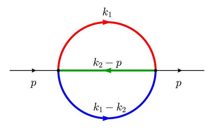
Figure 1: The unequal-mass sunrise diagram is shown above, where different colors represent different masses for the propagators. The only elliptic sector in the family is the top sector. The sub-sectors are obtained by pinching the propagators, which are double tadpoles. We will first consider the two unequal masses case and then move to the case with three unequal masses. These cases are well-studied in the literature Bogner:2019lfa ; Gorges:2023zgv .

The unequal masses sunrise diagram is shown in Fig. 1. The external legs are massive, and $D_{1}$, $D_{2}$ and $D_{3}$ are three massive propagators with distinctive masses shown in Fig. 1, while $D_{4}$ and $D_{5}$ are two ISPs, i.e., $v_{4}\leq 0,v_{5}\leq 0$. They are defined as

$$D_{1} =k_{1}^{2}-m_{1}^{2}\,,\quad D_{2} =(k_{2}-p)^{2}-m_{2}^{2}\,,\quad D_{3} =(k_{1}-k_{2})^{2}-m_{3}^{2}\,,$$ (57)

$$D_{4} =k_{2}^{2}\,,\quad D_{5} =(k_{1}-p)^{2}\,.$$

The integral family depends on masses $m_{i}$’s and the only Mandelstam variable associated with the incoming momentum $p$:

$$s\equiv p^{2}\,.$$ (58)

We have defined the integrals as dimensionless by introducing the scale $\mu^{2}$. We will choose $\mu^{2}=m_{1}^{2}$, such that the integrals are functions of the dimensionless variables

$$(x+y)^{2}\equiv\frac{4s}{m_{1}^{2}}\,,\quad(x-y)^{2}\equiv\frac{4m_{2}^{2}}{m_{1}^{2}}\,,\quad z^{2}\equiv\frac{m_{3}^{2}}{m_{1}^{2}}\,.$$ (59)

The definitions for dimensionless variables are chosen to make the branch points of the corresponding elliptic curves free of square roots, which we will see explicitly soon.

We use Kira Klappert:2020nbg to reduce the integrals in this family to a set of master integrals, chosen as

$$\big{\{}I_{11200}\,,I_{12100}\,,I_{21100}\,,I_{11100}\,,I_{01100}\,,I_{10100}\,,I_{11000}\big{\}}\,.$$ (60)

The first $4$ integrals are in the top sector, and we have $7$ master integrals in total. However, if we consider the case with two unequal masses, say, $m_{3}=m_{1}\neq m_{2}$. Then, $I_{11200}=I_{21100}$ and $I_{01100}=I_{11000}$ according to symmetric relations. Thus, we only have $3$ integrals in the top sector and $5$ master integrals in total. We will study the family in $d=2-2\varepsilon$, and only focus on the top sector since the non-elliptic sectors are trivial.

The maximal cut of the master integral $I_{11100}$ is given by

$${\rm MaxCut}[I_{11100}]=\int_{\cal C}\,u(z_{4}){\rm d}z_{4}\,,$$ (61)

where

$$u(z_{4})=P_{4}(z_{4})^{-1/2}\prod_{i=1}^{5}(z_{4}-c_{i})^{-\beta_{i}\varepsilon}\,.$$ (62)

The branch points can be expressed with the dimensionless variables as

$$c_{1}=(z-1)^{2}\,,\quad c_{2}=x^{2}\,,\quad c_{3}=y^{2}\,,\quad c_{4}=(z+1)^{2}\,,\quad c_{5}=0\,.$$ (63)

We first convert to the Legendre norm form and end up with the following variables by a Möbius transformation:

$$\lambda=\frac{4z(x^{2}-y^{2})}{[x^{2}-(z+1)^{2}][y^{2}-(z-1)^{2}]}\,,\quad e_{5}=\frac{4x^{2}z}{(z-1)^{2}[(z+1)^{2}-x^{2}]}\,,\quad e_{6}=\frac{4z}{(z+1)^{2}-x^{2}}\,.$$ (64)

For the two unequal masses case, $z$ degenerates to $1$ and the branch points become

$$c_{1}=0\,,\quad c_{2}=x^{2}\,,\quad c_{3}=y^{2}\,,\quad c_{4}=4\,.$$ (65)

The variables for the corresponding Legendre family are

$$\lambda=\frac{4(x^{2}-y^{2})}{(x^{2}-4)y^{2}}\,,\quad e=-\frac{4}{x^{2}-4}\,.$$ (66)

We consider the region $0<x<y<2$, $1<z<1+x$, and thus we have the order $c_{5}<c_{1}<c_{2}<c_{3}<c_{4}$. For concreteness, we consider the limit $x\to y^{-}$ where $\lambda\to 0$, and we only need the periods with subscript “$0$” in this limit.

3.1.2 Two unequal masses

We first consider the simpler case with two unequal masses. Following the construction in Sec. 2.2, the pre-canonical basis integrals are given by

$$\phi_{1}^{\rm sr2} =y\sqrt{4-x^{2}}\frac{{\rm d}z_{4}}{\sqrt{z_{4}(z_{4}-4)(z_{4}-x^{2})(z_{4}-y^{2})}}\,,$$ (67)

$$\phi_{2}^{\rm sr2} =-z\frac{{\rm d}z_{4}}{\sqrt{z_{4}(z_{4}-4)(z_{4}-x^{2})(z_{4}-y^{2})}}\,,$$ (68)

$$\phi_{3}^{\rm sr2} =\frac{4y(z-x^{2})}{z\sqrt{4-x^{2}}}\frac{{\rm d}z_{4}}{\sqrt{z_{4}(z_{4}-4)(z_{4}-x^{2})(z_{4}-y^{2})}}\,.$$ (69)

Next, we need to transform the pre-canonical basis to the canonical basis. The transformation ${\cal T}_{\rm can}$ is given in Sec. 2.3. The explicit form of the transformation can be obtained by plugging in the variables in Eq. (64). Applying the transformation, we find the corresponding connection matrix is automatically canonical and no further transformation is needed.

3.1.3 Three unequal masses

Following our procedure, we claim the case with three unequal masses is not substantially different from the previous case. The pre-canonical basis integrals are given by

$$\phi_{1}^{\rm sr3} =\sqrt{[(z+1)^{2}-x^{2}][y^{2}-(z-1)^{2}]}\frac{{\rm d}z_{4}}{\sqrt{[z_{4}-(z-1)^{2}][z_{4}-(z+1)^{2}](z_{4}-x^{2})(z_{4}-y^{2})}}\,,$$ (70)

$$\phi_{2}^{\rm sr3} =\frac{xy(z+1)[(z-1)^{2}-z_{4}]}{z_{4}(z-1)}\frac{{\rm d}z_{4}}{\sqrt{[z_{4}-(z-1)^{2}][z_{4}-(z+1)^{2}](z_{4}-x^{2})(z_{4}-y^{2})}}\,,$$ (71)

$$\phi_{3}^{\rm sr3} =[(z-1)^{2}-z_{4}]\frac{{\rm d}z_{4}}{\sqrt{[z_{4}-(z-1)^{2}][z_{4}-(z+1)^{2}](z_{4}-x^{2})(z_{4}-y^{2})}}\,,$$ (72)

$$\phi_{4}^{\rm sr3} =\frac{4z(x^{2}-z_{4})}{(z-1)^{2}-z_{4}}\sqrt{\frac{(y-z+1)(y+z-1)}{(z+1)^{2}-x^{2}}}\frac{{\rm d}z_{4}}{\sqrt{[z_{4}-(z-1)^{2}][z_{4}-(z+1)^{2}](z_{4}-x^{2})(z_{4}-y^{2})}}\,.$$ (73)

Similarly, we only need to apply the transformation to the canonical basis, and the mixing is $\varepsilon$-factorized automatically.

3.2 Non-planar double box

3.2.1 Definition

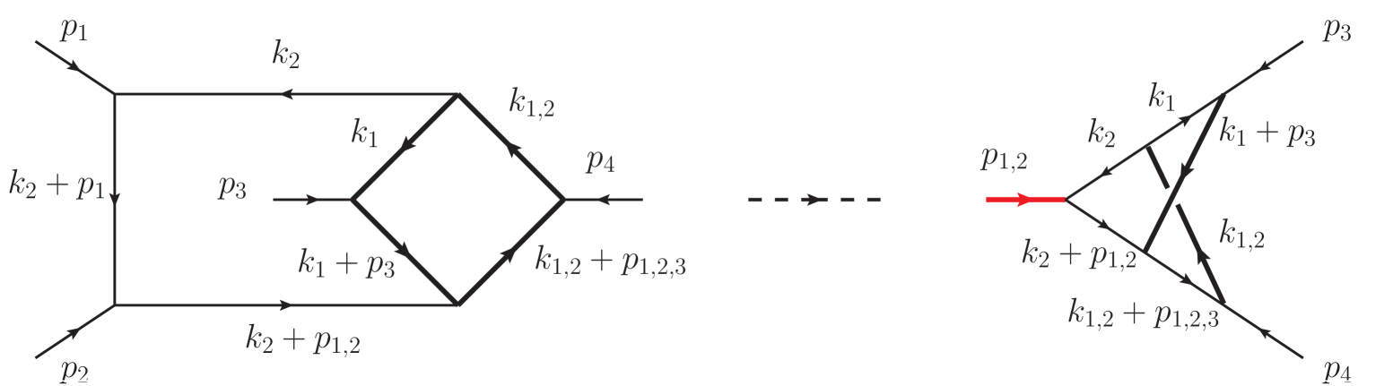
Figure 2: The non-planar double box diagram is shown in the left panel. The sub-sectors are obtained by pinching the propagators. A special case is the elliptic triangle sector, shown in the right panel. This sub-sector and the top sector are the only sectors that are elliptic, and they share the same elliptic curve. In the plot, thick lines are massive while all the others are massless, and we use the shorthand $p_{1,2,3}=p_{1}+p_{2}+p_{3}$ and $k_{1,2}=k_{1}+k_{2}$.

The non-planar double box diagram is shown in Fig. 2. All four external legs are massless and incoming, and it has a massive internal loop. $D_{1},\cdots,D_{7}$ are seven propagators, shown in Fig. 2, while $D_{8}$ and $D_{9}$ are two ISPs, i.e., $v_{8}\leq 0,v_{9}\leq 0$. They are defined as

$$D_{1} =k_{1}^{2}-m^{2}\,,\quad D_{2} =(k_{1}+p_{3})^{2}-m^{2}\,,$$ (74)

$$D_{3} =(k_{1}+k_{2}+p_{1}+p_{2}+p_{3})^{2}-m^{2}\,,\quad D_{4} =(k_{1}+k_{2})^{2}-m^{2}\,,$$

$$D_{5} =k_{2}^{2}\,,\quad D_{6} =(k_{2}+p_{1})^{2}\,,$$

$$D_{7} =(k_{2}+p_{1}+p_{2})^{2}\,,\quad D_{8} =(k_{1}-p_{1})^{2}-m^{2}\,,$$

$$D_{9} =(k_{2}+p_{1}+p_{3})^{2}\,.$$

We have the same propagators for the electroweak double box family, except $D_{1}$ and $D_{3}$ are massless. The integral family depends on the mass $m$ and two Mandelstam variables associated with the incoming momenta $p_{1}$, $p_{2}$ and $p_{3}$:

$$s\equiv\left(p_{1}+p_{2}\right)^{2},\quad t\equiv\left(p_{1}+p_{3}\right)^{2}.$$ (75)

We have defined the integrals as dimensionless by introducing the scale $\mu^{2}$. We will choose $\mu^{2}=s$, such that the integrals are functions of the dimensionless variables

$$y_{s}\equiv-\frac{m^{2}}{s},\quad y_{t}\equiv-\frac{t}{s}.$$ (76)

We use Kira Klappert:2020nbg to reduce the integrals in this family to a set of master integrals, chosen as

$$\big{\{} I_{111111100},I_{11111110(-1)},I_{21111110(-1)},I_{11121110(-1)},I_{111110100},I_{111210100},$$ (77)

$$I_{111101100},I_{111201100},I_{110111100},I_{111011100},I_{20101110(-1)},I_{201011100},$$

$$I_{010211100},I_{010111100},I_{110201100},I_{110101100},I_{111102000},I_{121101000},$$

$$I_{111101000},I_{201101100},I_{101101100},I_{111010100},I_{111100100},I_{102010200},$$

$$I_{102010100},I_{110200100},I_{110201000},I_{112001000},I_{002020100},I_{010202000},$$

$$I_{020201000},I_{200100200},I_{200200100},I_{201002000},I_{202001000},I_{022000000}\big{\}}\,.$$

The first 4 master integrals are in the top sector. They are chosen such that their differential equations have relatively simple dependencies on the (canonical) sub-sector integrals. This will be helpful in transforming these dependencies into the canonical form. The sub-sector integrals in the elliptic triangle family themselves are well-studied in the literature Jiang:2023jmk ; Gorges:2023zgv , where canonical bases have been constructed. For remaining sub-sector integrals, we construct the canonical basis integrals with ${\rm d}\log$-forms following Chen:2020uyk ; Chen:2022lzr , and the explicit expressions for them are in App. C. Alternative canonical bases for sub-sectors are also given in the literature, such as Ahmed:2024tsg ; Becchetti:2025rrz .

Here we have two sectors sharing the same elliptic curve in the family, and we find it enlightening to study the two elliptic sectors together by applying the elliptic (triangle) cut instead of the maximal cut of the top sector, under which only the two elliptic sectors survive. The elliptic cut of master integral $I_{111110100}$ is given by

$${\rm EllCut}[I_{111110100}]=\int_{\cal C}u(z_{6},z)\,{\rm d}z_{6}\wedge{\rm d}z\,,$$ (78)

where

$$u(z_{6},z)=P_{4}(z)^{-1/2}P_{2}(z_{6},z)^{-1/2}\prod_{i=1}^{4}(z-c_{i})^{-\beta_{i}\varepsilon}\prod_{j=6}^{7}(z_{6}-c_{j})^{-\beta_{j}\varepsilon}\,.$$ (79)

Branch points ${c_{1},c_{2},c_{3},c_{4}}$ can be expressed with kinematic variables $y_{s}$ and $y_{t}$ as

$$c_{1}=0\,,\quad c_{2}=\frac{1}{2}\left(1-\sqrt{1-16y_{s}}\right)\,,\quad c_{3}=\frac{1}{2}\left(1+\sqrt{1-16y_{s}}\right)\,,\quad c_{4}=1\,,$$ (80)

while branch points $c_{6}$ and $c_{7}$ also depend on variable $z$

$$c_{6,7}=2y_{t}z-y_{t}-z\pm 2\sqrt{y_{t}(y_{t}-1)z(z-1)}\,,$$ (81)

and $P_{2}(z_{6},z)$ is defined as

$$P_{2}(z_{6},z)=(z_{6}-c_{6})(z_{6}-c_{7})\,.$$ (82)

If we further apply the cut with respect to $z_{6}$, $c_{6}$ and $c_{7}$ degenerated to a single marked point $c_{5}$

$$\frac{1}{2i\pi}\oint_{z_{6}=0}\frac{1}{z_{6}\sqrt{P_{2}(z_{6},z)}}=-\frac{1}{z-c_{5}}\,,$$ (83)

where

$$c_{5}=y_{t}\,.$$ (84)

A Möbius transformation from the quartic form to the Legendre norm leads us to the following variables:

$$\lambda=\frac{4\sqrt{1-16y_{s}}}{\left(1+\sqrt{1-16y_{s}}\right)^{2}}\,,\quad e_{5}=\frac{\sqrt{1-16y_{s}}+2y_{t}-1}{\left(1+\sqrt{1-16y_{s}}\right)y_{t}}\,,\quad e_{6}=\frac{1-\sqrt{1-16y_{s}}}{8y_{s}}\,.$$ (85)

We need to introduce a complete elliptic integral of the third kind depending on $e_{6}$ for both sectors following Sec. 2.3. However, we have already known no such integral is needed in Jiang:2023jmk . We can find there are relations between complete elliptic integral of the first kind and the third kind

$$\vartheta_{0}(e_{6},\lambda)=-\frac{\varpi_{0}(\lambda)}{1+\sqrt{1-16y_{s}}}\,,\quad\vartheta_{1}(e_{6},\lambda)=-\frac{\varpi_{1}(\lambda)}{1+\sqrt{1-16y_{s}}}-1\,,$$ (86)

and their explicit forms can be simplified as

$$\Pi(k,k^{2})=\frac{1}{2}K(k^{2})+\frac{\pi}{4(1-k)}\,,\quad\Pi(1-k,1-k^{2})=\frac{(1+k)K(1-k^{2})}{2k}\,.$$ (87)

Similarly, branch points ${c_{1},c_{2},c_{3},c_{4}}$ for the electroweak double box family are given by

$$c_{1}=0\,,\quad c_{2}=\frac{(1-x)^{2}}{4}\,,\quad c_{3}=\frac{(1+x)^{2}}{4}\,,\quad c_{4}=1\,,$$ (88)

$c_{5}$, $c_{6}$ and $c_{7}$ are given by

$$c_{5}=y\,,\quad c_{6,7}=y(2z-1)-z\pm 2\sqrt{y(y-1)z(z-1)}\,,$$ (89)

where we define new variables $x$ and $y$ to simplify the expressions

$$x\equiv\sqrt{1-8y_{s}}\,,\quad y\equiv 1-y_{t}\,.$$ (90)

The variables relevant in the Legendre norm form are

$$\lambda=\frac{16x}{(3-x)(1+x)^{3}}\,,\quad e_{5}=\frac{4y-x^{2}+2x-1}{y(3-x)(1+x)}\,,\quad e_{6}=\frac{4}{(3-x)(1+x)}\,.$$ (91)

One can deduce there must exist special relations like Eqs. (86) and (87) for the same reason, which are

$$\vartheta_{0}(e_{6},\lambda)=-\frac{(x^{2}+3)\varpi_{0}(\lambda)}{3(1+x)\sqrt{(3-x)(1+x)}}\,,\quad\vartheta_{1}(e_{6},\lambda)=-\frac{(x^{2}+3)\varpi_{1}(\lambda)}{3(1+x)\sqrt{(3-x)(1+x)}}-\frac{4}{3}\,.$$ (92)

The explicit forms are

$$\Pi\left(\frac{4x}{(1+x)^{2}},\frac{16x}{(3-x)(1+x)^{3}}\right) =\frac{x^{2}+3}{3(1-x)^{2}}K\left(\frac{16x}{(3-x)(1+x)^{3}}\right)\,,$$ (93)

$$\Pi\left(\frac{(1-x)(3+x)}{(3-x)(1+x)},1-\frac{16x}{(3-x)(1+x)^{3}}\right) =\frac{3-x}{6}K\left(1-\frac{16x}{(3-x)(1+x)^{3}}\right)+\frac{\pi(3-x)(1+x)^{2}}{12x\sqrt{(3-x)(1+x)}}\,.$$ (94)

We will mainly study the behaviors of the integrals in the vicinity of the degenerate point $m^{2}\to 0^{-}$ (as in Jiang:2023jmk ), where the order of the branch points is $c_{1}<c_{2}<c_{3}<c_{4}$ and we have $y_{s}\to 0$, $\lambda\to 1$. The vicinity of the degenerate point $s\to-16m^{2}$ (corresponding to $y_{s}\to 1/16$ and $\lambda\to 0$) can be studied similarly. For the study of the point $s\to 0$, it is better to modify the normalization of the integrals in Eq. (1) by setting $\mu^{2}=m^{2}$.

Note that the shape of the elliptic curve and the integrals in the triangle sub-sector only depend on the kinematic variable $y_{s}$. This is why the maximal cut of the triangle integrals can be characterized by modular forms. The integrals in the top sector, on the other hand, depend on the variable $y_{t}$ as well. This leads to extra complications in the construction of canonical bases. In the next two subsubsections, we first consider the construction of a pre-canonical basis under the elliptic (triangle) cut with nice properties, then apply the transformation ${\cal T}_{\rm can}^{(\varepsilon)}$ to remove residual non-$\varepsilon$-factorized elements, and finally transform the differential equations to a canonical form with ${\cal T}_{\rm can}^{(0)}$.

3.2.2 Transformation for the elliptic sectors

We note that the elliptic cut of $I_{111110100}$ can be written as

$${\rm EllCut}[I_{111110100}]=\int_{\cal C}\,\bar{u}(z_{6},z)\frac{{\rm d}z_{6}}{\sqrt{P_{2}(z_{6},z)}}\wedge\frac{{\rm d}z}{\sqrt{P_{4}(z)}}=-\int_{\cal C}\,\bar{u}(z_{6},z){\rm d}\log\left(\frac{1+\sqrt{\frac{z_{6}-c_{6}}{z_{6}-c_{7}}}}{1-\sqrt{\frac{z_{6}-c_{6}}{z_{6}-c_{7}}}}\right)\wedge\frac{{\rm d}z}{\sqrt{P_{4}(z)}}\,,$$ (95)

where $\bar{u}(z_{6},z)$ is the reduced twist

$$\bar{u}(z_{6},z)=\prod_{i=1}^{4}(z-c_{i})^{-\beta_{i}\varepsilon}\prod_{j=6}^{7}(z_{6}-c_{j})^{-\beta_{j}\varepsilon}\,.$$ (96)

Similarly, we have

$${\rm EllCut}[I_{111111100}] =\int_{\cal C}\,\bar{u}(z_{6},z)\frac{{\rm d}z_{6}}{z_{6}\sqrt{P_{2}(z_{6},z)}}\wedge\frac{{\rm d}z}{\sqrt{P_{4}(z)}}$$ (97)

$$=\int_{\cal C}\,\bar{u}(z_{6},z){\rm d}\log\left(\frac{1+\sqrt{\frac{c_{7}(z_{6}-c_{6})}{c_{6}(z_{6}-c_{7})}}}{1-\sqrt{\frac{c_{7}(z_{6}-c_{6})}{c_{6}(z_{6}-c_{7})}}}\right)\wedge\frac{{\rm d}z}{(z-c_{5})\sqrt{P_{4}(z)}}\,.$$ (98)

From Eqs. (95) and (97), we can see explicitly that they share the same elliptic curve defined by $w^{2}=P_{4}(z)$, and a natural idea is to construct the pre-canonical basis integrals as ${\rm d}\log\wedge\phi$.

Following the construction in Sec. 2, the four pre-canonical basis integrals in the top sector can be defined with

$$\phi_{1}^{\rm npdb} =\frac{1}{2}\left(1+\sqrt{1-16y_{s}}\right)\frac{{\rm d}z}{\sqrt{z(z-1)[z(z-1)+4y_{s}]}}\,,$$ (99a)

$$\phi_{2}^{\rm npdb} =\frac{z\sqrt{(y_{t}-1)y_{t}[4y_{s}+(y_{t}-1)y_{t}]}}{y_{t}(z-y_{t})}\frac{{\rm d}z}{\sqrt{z(z-1)[z(z-1)+4y_{s}]}}\,,$$ (99b)

$$\phi_{3}^{\rm npdb} =-z\frac{{\rm d}z}{\sqrt{z(z-1)[z(z-1)+4y_{s}]}}\,,$$ (99c)

$$\phi_{4}^{\rm npdb} =\frac{z-\frac{1}{2}\left(1-\sqrt{1-16y_{s}}\right)}{z}\frac{{\rm d}z}{\sqrt{z(z-1)[z(z-1)+4y_{s}]}}\,,$$ (99d)

for electroweak double box

$$\phi_{1}^{\rm ewdb} =(1+x)\sqrt{(3-x)(1+x)}\frac{{\rm d}z}{\sqrt{z(z-1)[4z-(1-x)^{2}][4z-(1+x)^{2}]}}\,,$$ (100a)

$$\phi_{2}^{\rm ewdb} =\frac{z\sqrt{y(y-1)[x^{4}-2(1+4y)x^{2}+(1-4y)^{2}]}}{y(z-y)}\frac{{\rm d}z}{\sqrt{z(z-1)[4z-(1-x)^{2}][4z-(1+x)^{2}]}}\,,$$ (100b)

$$\phi_{3}^{\rm ewdb} =-4z\frac{{\rm d}z}{\sqrt{z(z-1)[4z-(1-x)^{2}][4z-(1+x)^{2}]}}\,,$$ (100c)

$$\phi_{4}^{\rm ewdb} =\frac{\sqrt{(3-x)(1+x)}}{3-x}\frac{4z-x^{2}+2x-1}{z}\frac{{\rm d}z}{\sqrt{z(z-1)[4z-(1-x)^{2}][4z-(1+x)^{2}]}}\,.$$ (100d)

For the triangle sector, we only need to pick the first and the last ones. Moreover, we find that if we further change the integral of the second kind, namely, $\phi^{\rm npdb}_{4}$, with the derivative of the first kind $\phi^{\rm npdb}_{1}$ with respect to $y_{s}$, and then apply the transformations to the canonical bases for top sector and triangle sector, the mixing is $\varepsilon$-factorized as well. We note that the derivative basis cannot promise the $\varepsilon$-factorization for the electroweak family, but it is very close to so that we can achieve it with a simple transformation.

We would like to give short comments on the procedure above. Here, we want to construct a canonical basis for the whole elliptic sectors instead of sector by sector or, say, block by block, respectively. Our strategy is to try constructing basis integrals in the form ${\rm d}\log\wedge\phi$. In this way, the corresponding projection transformation contains more information in the mixing between sectors, which cannot be seen from separate maximal cuts. Moreover, it turns out that no further transformation is necessary for integrals of the first kind and the third kind. Similar to the case under the maximal cut, the integral of the second kind is always the most complicated one and it seems that by assigning it with the derivative basis of the first kind integral, the mixing becomes simpler. Specially, for the first family, simply using the derivative with respect to $y_{s}$ is enough. A more natural choice is the derivative with respect to $\lambda$ (and the other variable is $e_{5}$), but it is not as simple as $y_{s}$ in this case. Further transformation is needed. The simplicity with respect to $y_{s}$ is, in fact, an accident since it is not enough for the electroweak cousin of this family. Another point is the additional transformation is only dependent on the first kind of the triangle family. However, the two cases are very similar, and thus, one needs to check further non-trivial examples for this observation.

3.2.3 Mixing with non-elliptic sectors

Here we go on to find the canonical basis for the first family without cuts. As mentioned before, it is sometimes simpler to work with a pre-canonical basis instead of the canonical basis since there are no elliptic integrals in a pre-canonical basis. If we manage to make the mixing with non-elliptic sub-sectors for integrals of the first and the third kind $\varepsilon$-factorized, the same structure will be preserved in canonical basis, with applying ${\cal T}_{\rm can}$ or ${\cal T}_{\rm can}^{(\varepsilon)}$. Thus, we only need to modify the integral of the second kind later. Usually, we need not introduce elliptic integrals to make a pre-canonical basis satisfy this property, which makes the work simpler. Here we would like to show an example.

Provided with the canonical basis integrals in the elliptic sectors, we restore top sector integrals back to pre-canonical ones and then the structure of the coefficient matrix $\bm{A}$ can be presented schematically as

$$\left(\begin{array}[]{cccc}\pagecolor{Purple}A_{11}&\pagecolor{cyan}A_{12}&\pagecolor{cyan}A_{13}&\pagecolor{red}A_{14}\\ \pagecolor{Purple}A_{21}&\pagecolor{cyan}A_{22}&\pagecolor{cyan}A_{23}&\pagecolor{red}A_{24}\\ \pagecolor{Purple}A_{31}&\pagecolor{cyan}A_{32}&\pagecolor{cyan}A_{33}&\pagecolor{red}A_{34}\\ \pagecolor{Purple}A_{41}&\pagecolor{cyan}A_{42}&\pagecolor{cyan}A_{43}&\pagecolor{Purple}A_{44}\end{array}\right)\,,$$ (101)

where the cyan cells are already $\varepsilon$-factorized, the purple cells are linear in $\varepsilon$, and the red cells contain only $\varepsilon^{0}$ terms.

There is only one element ${\bm{A}}_{4,8}$ containing $\varepsilon^{0}$-term in the mixing for $I_{4}$ with non-elliptic sub-sectors, and we apply an ansatz transformation to remove it

$$I_{1}\to I_{1}+f_{1,8}(y_{s},y_{t})M_{8}\,,\quad I_{4}\to I_{4}+f_{4,8}(y_{s},y_{t})M_{8}\,,$$ (102)

where the solutions are given by

$$f_{1,8}(y_{s},y_{t})=-\frac{4(1+\sqrt{1-16y_{s}})(2y_{t}-1)}{\sqrt{y_{s}(y_{t}-1)y_{t}}}\,,\quad f_{4,8}(y_{s},y_{t})=-\frac{8\sqrt{1-16y_{s}}(2y_{t}-1)}{(1+\sqrt{1-16y_{s}})\sqrt{y_{s}(y_{t}-1)y_{t}}}\,.$$ (103)

Now all the mixing elements ${\bm{A}}_{4,j}$’s for $(j=7,\cdots,36)$ are in the forms $a^{(1)}\varepsilon+a^{(2)}\varepsilon^{2}$, and ${\bm{A}}_{1,j}$’s are all $\varepsilon$-factorized while ${\bm{A}}_{2/3,j}$’s are in linear forms $a^{(0)}+a^{(1)}\varepsilon$. According to (101), all the $A_{m,2/3}$’s are $\varepsilon$-factorized, and thus we can apply ansatz transformations for $I_{2/3}$

$$I_{2/3}\to I_{2/3}+f_{2/3,j}(y_{s},y_{t})M_{j}\,,$$ (104)

with which we can remove ${\bm{A}}_{2/3,j}^{(0)}$, without altering the $\varepsilon$-factorized structures for $I_{1}$ and $I_{4}$.

Then, we only need to modify the integral of the second kind, namely, $I_{4}$. We apply transformation ${\cal T}_{\rm can}^{(\varepsilon)}$, where non-$\varepsilon$-factorized elements in the corresponding connection matrix for the top sector are strictly lower triangular. The mixing for the integral of the second kind are all in the linear forms $a^{(0)}+a^{(1)}\varepsilon$, and if we remove all the $\varepsilon^{0}$-terms, the connection matrix is promised to be canonical directly with a further ${\cal T}_{\rm can}^{(0)}$.

The $\varepsilon^{0}$-terms can be removed with regular “integrating out” strategy, and it turns out there are no new functions needed in the transformation beyond the periods $\varpi_{0}(\lambda)$ and $\vartheta_{0}(e_{5},\lambda)$ in ${\cal T}_{\rm can}$. For simplicity, we suppress the explicit expressions here and they can be found in ancillary files.

4 Conclusion and outlook

In this paper, we develop a systematic method to construct a canonical basis for elliptic Feynman integral families involving multiple kinematic scales, which exhibit a univariate integral in the Baikov representation under maximal cut. The core idea is to perform the construction using the Legendre normal form of elliptic curves, where the geometric information is explicit, and the apply a Möbius transformation to map it back to the original integral family. The pre-canonical basis integrals under maximal cut are expressed as linear combinations of Abelian differentials, without elliptic integrals in the combination coefficients. This feature provides simplification when performing the $\varepsilon$-factorization for the dependence on sub-sectors. Furthermore, the canonical bases exhibit favorable behaviors around chosen degenerate points, where they asymptotically take the ${\rm d}\log$-forms. This helps to obtain simple boundary conditions for the differential equations. Around the degenerate point, only the dependence of the basis integrals on the marked points becomes significant, allowing the integrals to be expressed in terms of MPLs in this context.

There can be different ways in the construction of the pre-canonical bases and the transformations bringing them to the canonical ones. Besides the method described in the main text, we have explored several other possibilities which are described in the appendices. In App. A, we show that our pre-canonical basis can be transformed to a canonical one by converting the period matrix into a constant matrix without $\varepsilon$-dependent transformation vonManteuffel:2017hms ; Frellesvig:2021hkr . Despite a simpler $\varepsilon$-dependence, this method introduces numerous elliptic integrals into the transformation, which, in turn, appear in the $\varepsilon$-factorized differential equations. In addition, this approach inherently leads to the transformation with logarithmic behaviors near degenerate points due to the complementary arguments $\lambda$ and $1-\lambda$ in elliptic integrals of the first and second kinds. Relevant discussions are included in Frellesvig:2023iwr . In contrast, the approach that we take avoids these issues, and the resulting canonical bases satisfy most of the nice properties advocated in Dlapa:2022wdu ; Frellesvig:2023iwr ; Duhr:2024uid .

To demonstrate our method, we use fully massive sunrise families and the non-planar double-box families with an internal mass as a proof of concept. Our method is similar to those in vonManteuffel:2017hms ; Adams:2018bsn ; Frellesvig:2021hkr ; Giroux:2022wav ; Dlapa:2022wdu ; Pogel:2022vat ; Gorges:2023zgv , but provides a more streamline framework for the construction. With the universal construction in the normal form, the results can be readily applied to generic elliptic integral families. Moreover, since the proposed approach is not inherently limited to elliptic cases, it is expected to extend to more complex geometries, e.g., hyperelliptic cases, as explored in the recent work Duhr:2024uid . For example, using the canonical basis integrals constructed for the four-parameter Lauricella functions, combined with an appropriate Möbius transformation, one may derive the canonical basis for the equal-mass non-planar double (crossed) box family, at least under the maximal cut. One can also try constructing a canonical basis in suitable (Rosenhain) normal form family with kinematic marked points, which can be potentially applied for generic hyperelliptic (of fixed genus) Feynman integrals, with suitable Möbius transformations.

Our method can be applied to integral families where multiple sectors involve the same elliptic curve. In such cases, the construction can be done sector-by sector. However, we have found that it is helpful to perform the construction for these sectors together by loosening the maximal cut. This has been demonstrated for the non-planar double box family in Sec. 3.2, where both the top-sector and one of the triangle sectors are elliptic. It remains possible that one may construct the full integrand without any cut, combining the elliptic-sector construction in this work and the ${\rm d}\log$-form construction in Chen:2020uyk ; Chen:2022lzr . It is also interesting to explore the application of our method to cases where multiple elliptic curves are involved. In this case, there can be non-trivial interplays among the Abelian differentials in different elliptic sectors, and it is interesting to see how these can be handled within our approach. Another complication arises in the boundary conditions, since the degenerate points of the different elliptic curves may not coincide. It remains to be seen whether one may utilize the degenerate information separately, and connect them via the differential equations. We leave these for future investigations.

Appendix A Construct $\varepsilon$-factorized basis with constant period matrix

In Sec. 2.3, we apply the derivative basis method Pogel:2022vat to construct the canonical basis. However, it is not the only method to find an $\varepsilon$-factorized basis. With a pre-canonical basis whose connection matrix in a special linear form, we can also try the strategy in vonManteuffel:2017hms ; Frellesvig:2021hkr .

As already pointed out in Sec. 2.2, the general structure of $\bm{A}^{(0)}$ motivates us to do the following linear transformation

$$\phi_{i-3}\to\big{(}\,\mathcal{T}_{1}.\vec{\phi}\,\big{)}_{i-3}=\phi_{i-3}+\left[F(\sin^{-1}a_{i},\lambda)-E(\sin^{-1}a_{i},\lambda)\right]\phi_{1}-F(\sin^{-1}a_{i},\lambda)\phi_{n-1}\,,$$ (105)

for $5\leq i\leq n+1$, with $a_{i}=\sqrt{e_{i}/\lambda}$, and we have implicitly introduced the rotation matrix $\mathcal{T}_{1}$ acting on the basis. The transformation carries over to the integral level, namely, $I_{i-3}\to\big{(}\,\mathcal{T}_{1}.\vec{I}\,\big{)}_{i-3}$, and we will suppress it for brevity. After such a transformation, it is straightforward to verify that the derivatives (with respect to $\lambda$ or $e_{i}$) of master integrals $I_{j}$’s with $3\leq j\leq n-2$, are $\varepsilon$-factorized under the maximal cut.

Now, the remaining task is to further transform $\phi_{1}$ and $\phi_{n-1}$, to rotate the corresponding $2\times 2$ block of $\bm{A}^{(0)}$ away, which is only $\lambda$ relevant. To do that, we only need to consider the corresponding $2\times 2$ block of the period matrix for $\phi_{1}$ and $\phi_{n-1}$, which is

$${\cal P} =\begin{pmatrix}2K(\lambda)&-2iK(1-\lambda)\\ 2K(\lambda)-2E(\lambda)&-2iE(1-\lambda)\end{pmatrix}\,.$$ (106)

We can see the matrix elements involve linear combinations of the complete elliptic integrals of the first and second kinds. They can be rotated to constants with the help of the well-known Legendre relation. A possible rotation matrix is given by

$${\cal T}_{2}=\begin{pmatrix}E(1-\lambda)&0&\cdots&0&-K(1-\lambda)\\ 0&1&\cdots&0&0\\ \vdots&\vdots&\ddots&\vdots&\vdots\\ 0&0&\cdots&1&0\\ E(\lambda)-K(\lambda)&0&\cdots&0&K(\lambda)\end{pmatrix}\,.$$ (107)

After the rotation, we can easily see that the period matrix becomes a constant matrix. It is easy to check that the differential equations within the top sector are now $\varepsilon$-factorized after the transformations. The full transformation matrix from the pre-canonical basis to the $\varepsilon$-factorized basis is given by

$${\cal T}={\cal T}_{2}\cdot{\cal T}_{1}=\begin{pmatrix}E(1-\lambda)&0&\cdots&0&-K(1-\lambda)\\ F(\sin^{-1}a_{5},\lambda)-E(\sin^{-1}a_{5},\lambda)&1&\cdots&0&-F(\sin^{-1}a_{5},\lambda)\\ \vdots&\vdots&\ddots&\vdots&\vdots\\ F(\sin^{-1}a_{\infty},\lambda)-E(\sin^{-1}a_{\infty},\lambda)&0&\cdots&1&-F(\sin^{-1}a_{\infty},\lambda)\\ E(\lambda)-K(\lambda)&0&\cdots&0&K(\lambda)\end{pmatrix}\,.$$ (108)

We’ve briefly discussed the asymptotic behaviors of the pre-canonical basis in the degenerate limit $c_{1}\to c_{2}$ or $\lambda\to 1$. It’s natural to consider the asymptotic behaviors of the $\varepsilon$-factorized basis as well. It suffices to study the asymptotic behaviors of the elliptic integrals appearing in the transformation matrices ${\cal T}_{1}$ and ${\cal T}_{2}$. We have the following:

$$\lim_{\lambda\to 1}K(1-\lambda)=\lim_{\lambda\to 1}E(1-\lambda)=\frac{\pi}{2}\,,$$ (109)

$$\lim_{\lambda\to 1}E(\lambda)=1\,,\qquad\lim_{\lambda\to 1}K(\lambda)=\infty\,,$$

$$\lim_{c_{1}\to c_{2}}E(\sin^{-1}a_{i},\lambda)=\lim_{\lambda\to 1}E(\lambda)=1\,,$$

$$\lim_{c_{1}\to c_{2}}F(\sin^{-1}a_{i},\lambda)=\lim_{\lambda\to 1}K(\lambda)=\infty\,.$$

Note that $K(\lambda)$ and $F(\sin^{-1}a_{i},\lambda)$ are singular as $c_{1}\to c_{2}$, and they are logarithmically singular in this limit. These singularities do not cause problems for the basis integrals, since they cancel due to the fact that $\phi_{1}=\phi_{2}$ when $c_{1}\to c_{2}$; see Eq. (53). This cancellation also implies that the first $\varepsilon$-factorized basis integral vanishes in this limit. Similar to the pre-canonical basis, other $\varepsilon$-factorized basis integrals are ${\rm d}\log$-forms asymptotically in the neighborhood of the degenerate points $c_{1}=c_{2}$, as desired. From the demonstration above, we can see the construction in Sec. 2.3 is essentially different from the procedure here from two related perspectives. On the one hand, we introduce $\varepsilon$-dependence in the fiber transformations in the former construction, while the construction here does not. On the other hand, there are only complete elliptic integrals with a unique modulus arguments in the former case, while here we introduce incomplete elliptic integrals and both of complementary moduli arguments are needed. As a consequence, the construction here will introduce more elliptic integrals and undesirable asymptotic properties for the transformation. More relevant discussions can also be found in Frellesvig:2023iwr .

Appendix B Canonical basis with Jacobi normal form

We construct the pre-canonical basis and the corresponding canonical basis with the elliptic curve in Legendre normal form in Sec. 2. From there, we know the explicit dependence on shape of the curve encoded in the parameter $\lambda$ makes our construction simple. There is another special normal form named Jacobi normal form shares similar feature with Legendre normal form. Thus, a natural question is why not try constructing the basis in Jacobi form. In this appendix, we will demonstrate the construction of pre-canonical basis and canonical basis in Jacobi normal form.

The elliptic curve in Jacobi normal form is given by

$$v^{2}\equiv P_{J}(t)\equiv k^{2}\,P_{4J}(t)=(1-t^{2})(1-k^{2}t^{2})\,.$$ (110)

The twist is

$$u_{J}(t)=P_{4J}(t)^{-1/2}\prod_{i=1}^{n}(t-a_{i})^{-\beta_{i}\varepsilon}\,,$$ (111)

with $a_{1}=-1/k$, $a_{2}=-1$, $a_{3}=1$ and $a_{4}=1/k$. We also denote

$$\beta_{n+1}\equiv\beta_{\infty}\equiv-\sum_{i=1}^{n}\beta_{i}\,,$$ (112)

and

$$\phi=\frac{\varphi}{\sqrt{P_{4J}(t)}}\,,$$ (113)

for convenience.

Since the idea is basically the same as the one in the main text, we will keep the contents concise.

B.1 The pre-canonical basis

B.1.1 The construction of pre-canonical basis in the Jacobi form

Similar to the strategy in Sec. 2.2, we consider pre-canonical basis integrals as the elliptic integrals of the three kinds in the Jacobi form

$$\phi_{1} =\frac{{\rm d}t}{\sqrt{P_{J}(t)}}={\rm d}K(\sin^{-1}t,k^{2})\,,$$ (114a)

$$\phi_{i-3} =\frac{1}{t-a_{i}}\frac{\sqrt{P_{J}(a_{i})}}{\sqrt{P_{J}(t)}}{\rm d}t=\frac{1}{2}{\rm d}\log\left(\frac{1+\sqrt{\frac{(1-t^{2})(1-k^{2}a_{i}^{2})}{(1-a_{i}^{2})(1-k^{2}t^{2})}}}{1-\sqrt{\frac{(1-t^{2})(1-k^{2}a_{i}^{2})}{(1-a_{i}^{2})(1-k^{2}t^{2})}}}\right)-\frac{\sqrt{P_{J}(a_{i})}}{a_{i}}{\rm d}\Pi(1/a_{i}^{2},\sin^{-1}t,k^{2})\,,$$ (114b)

$$\phi_{n-2} =\frac{t}{\sqrt{P_{4J}(t)}}{\rm d}t=\frac{1}{2}{\rm d}\log\left(\frac{1+k\sqrt{\frac{1-t^{2}}{1-k^{2}t^{2}}}}{1-k\sqrt{\frac{1-t^{2}}{1-k^{2}t^{2}}}}\right)\,,$$ (114c)

$$\phi_{n-1} =\frac{1-k^{2}t^{2}}{\sqrt{P_{J}(t)}}{\rm d}t={\rm d}E(\sin^{-1}t,k^{2})\,,$$ (114d)

where $i=5,\cdots,n$ and the next to last basis differential $\phi_{n-2}$ is a ${\rm d}\log$-form. Then we can find that the differential equation is in a special linear form. The $\varepsilon^{0}$-part of the connection matrix with respect to $k$ is

$$\begin{pmatrix}-\frac{1}{k}&0&\cdots&0&\frac{1}{k(1-k^{2})}\\ 0&0&\cdots&0&-\frac{a_{5}(a_{5}^{2}-1)k}{(1-k^{2})\sqrt{P_{J}(a_{5})}}\\ \vdots&\vdots&\ddots&\vdots&\vdots\\ 0&0&\cdots&0&-\frac{a_{n}(a_{n}^{2}-1)k}{(1-k^{2})\sqrt{P_{J}(a_{n})}}\\ 0&0&\cdots&0&0\\ -\frac{1}{k}&0&\cdots&0&\frac{1}{k}\end{pmatrix}\,,$$ (115)

while the one with respect to $a_{i}$ is

$$\begin{pmatrix}0&0&\cdots&0&0\\ \vdots&\vdots&\ddots&\vdots&\vdots\\ -\frac{a_{i}^{2}k^{2}-1}{\sqrt{P_{J}(a_{i})}}&0&\cdots&0&-\frac{1}{\sqrt{P_{J}(a_{i})}}\\ \vdots&\vdots&\ddots&\vdots&\vdots\\ 0&0&\cdots&0&0\end{pmatrix}\,,$$ (116)

for $i=5,\cdots,n$. We can see the non-zero elements only appear in the first and the last columns, similar to the ones in Sec. 2.2.

B.2 The canonical basis

In this subsection, we focus on constructing a canonical basis based on the pre-canonical basis in App. B.1 under the maximal cut then towards the fully $\varepsilon$-factorized basis of the family. Similar to the Legendre family, we consider both of the two methods, with derivative basis in App. B.2.1 and constant period matrix in App. B.2.2.

B.2.1 The construction with derivative basis

The periods are

$$\varpi_{0}(k)\equiv\frac{2}{\pi}\int_{-1}^{1}\frac{{\rm d}t}{\sqrt{P_{J}(t)}}=\frac{4}{\pi}K(k^{2})\,,\quad\varpi_{1}(k)\equiv\frac{2i}{\pi}\int_{1}^{\frac{1}{k}}\frac{{\rm d}t}{\sqrt{P_{J}(t)}}=\frac{2}{\pi}K(1-k^{2})\,,$$ (117)

where $\varpi_{0}(k)$ and $\varpi_{1}(k)$ are holomorphic around degenerate points $k=0$ and $k=1$, respectively. The modular $\tau$ is defined as

$$\tau\equiv\frac{i\varpi_{1}(k)}{\varpi_{0}(k)}=\frac{iK(1-k^{2})}{2K(k^{2})}\in{\mathbb{H}}\,.$$ (118)

The corresponding derivative basis integrals are

$$\tilde{I}_{1}=\frac{1}{\varpi_{0}(k)}I_{1}\,,\quad\tilde{I}_{n-1}=\frac{1}{\varepsilon}\frac{\varpi_{0}(k)^{2}}{\pi W_{k}}\partial_{k}\tilde{I}_{1}\,,$$ (119)

where $W_{k}$ is the Wronskian of $\varpi_{0}$ and $\varpi_{1}$ with respect to $k$

$$W_{k}=\varpi_{0}\partial_{k}\varpi_{1}-\varpi_{1}\partial_{k}\varpi_{0}=-\frac{4}{\pi k(1-k^{2})}\,.$$ (120)

The non-trivial elements in the transformation from pre-canonical basis $\vec{I}$ to $\tilde{\vec{I}}$ as ${\cal T_{\rm der}}$ are

$$({\cal T}_{\rm der})_{1,1} =\frac{1}{\varpi_{0}(k)}\,,$$ (121a)

$$({\cal T}_{\rm der})_{n-1,n-1} =-\frac{1+\beta_{n+1}\varepsilon}{4\varepsilon}\varpi_{0}(k)\,,$$ (121b)

$$({\cal T}_{\rm der})_{n-1,j} =-\frac{1}{4}\beta_{j+3}\frac{a_{j+3}(a_{j+3}^{2}-1)k^{2}}{\sqrt{P_{J}(a_{j+3})}}\varpi_{0}(k)\,,$$ (121c)

$$({\cal T}_{\rm der})_{n-1,n-2} =-\frac{1}{4}k\varpi_{0}(k)\sum_{i=1}^{n}\beta_{i}a_{i}\,,$$ (121d)

$$({\cal T}_{\rm der})_{n-1,1} =\frac{1}{4\varepsilon}\left\{(1-k^{2})\varpi_{0}(k)+k(1-k^{2})\varpi_{0}^{\prime}(k)-\varepsilon\sum_{i=1}^{n}\beta_{i}[1+k^{2}(a_{i}^{2}-1)]\varpi_{0}(k)\right\}\,,$$ (121e)

where $2\leq j\leq n-3$ and other diagonal elements are equal to $1$. The non-zero elements in the coefficient matrix of ${\rm d}a_{i}$ in $\tilde{\bm{A}}^{(0)}$ are given by

$$(\tilde{\bm{A}}^{(0)}_{a_{i}})_{i-3,1} =-\frac{k[k(a_{i}^{2}-1)\varpi_{0}(k)+(1-k^{2})\varpi_{0}^{\prime}(k)]}{\sqrt{P_{J}(a_{i})}}\,,$$ (122a)

$$(\tilde{\bm{A}}^{(0)}_{a_{i}})_{n-1,1} =\beta_{i}\frac{a_{i}k^{2}(1-k^{2})[\varpi_{0}(k)+k\varpi^{\prime}_{0}(k)]\varpi_{0}(k)}{4(a_{i}^{2}k^{2}-1)}\,,$$ (122b)

$$(\tilde{\bm{A}}^{(0)}_{a_{i}})_{n-1,i-3} =\beta_{i}\frac{k(1-k^{2})[a_{i}^{2}k\varpi_{0}(k)+(a_{i}^{2}k^{2}-1)\varpi^{\prime}_{0}(k)]}{4(a_{i}^{2}k^{2}-1)\sqrt{P_{J}(a_{i})}}\,.$$ (122c)

Elements $(\tilde{\bm{A}}^{(0)}_{a_{i}})_{i-3,1}$ can be removed with function $\vartheta_{0}(a_{i},k)$, and its explicit form is given by

$$\vartheta_{0}(a_{i},k)\equiv-\frac{4\sqrt{P_{J}(a_{i})}}{\pi a_{i}}\Pi(1/a_{i}^{2},k^{2})\,,$$ (123)

and its counterpart $\vartheta_{1}(a_{i},k)$ is

$$\vartheta_{1}(a_{i},k)\equiv-\frac{2\sqrt{P_{J}(a_{i})}}{\pi a_{i}}\left[K(1-k^{2})+\frac{1}{a_{i}^{2}-1}\Pi\left(\frac{a_{i}^{2}(1-k^{2})}{a_{i}^{2}-1},1-k^{2}\right)\right]\,.$$ (124)

The non-trivial elements in the transformation ${\cal T}$ from the pre-canonical basis $\tilde{\vec{I}}$ are

$${\cal T}_{j,1} =-\vartheta_{0}(a_{j+3},k)\,,$$ (125a)

$${\cal T}_{n-1,j} =\frac{1}{4}\beta_{j+3}\left[\vartheta_{0}(a_{j+3},k)+\frac{a_{j+3}(a_{j+3}^{2}-1)k^{2}\varpi_{0}(k)}{\sqrt{P_{J}(a_{j+3})}}\right]\,,$$ (125b)

$${\cal T}_{n-1,1} =-\frac{1}{8}\left\{\sum_{i=5}^{n}\beta_{i}\vartheta_{0}(a_{i},k)^{2}-\sum_{i=1}^{n}\beta_{i}[1+k^{2}(a_{i}^{2}-1)]\varpi_{0}(k)^{2}\right\}\,,$$ (125c)

where diagonal elements are equal to $1$. With ${\cal T}_{\rm der}$ from (33) and ${\cal T}$ from (38), the transformation from pre-canonical basis $\vec{I}$ to canonical basis ${\cal T}_{\rm can}$ can be obtained directly

$${\cal T}_{\rm can}={\cal T}\cdot{\cal T}_{\rm der}\,.$$ (126)

The canonical basis and the corresponding connection matrix here share similar properties as the ones in the main text in Legendre family.

We can decompose the total transformation ${\cal T}_{\rm can}$ into an $\varepsilon$-dependent part and an $\varepsilon$-independent part as

$${\cal T}_{\rm can}={\cal T}_{\rm can}^{(0)}\cdot{\cal T}_{\rm can}^{(\varepsilon)}\,,$$ (127)

where

$${\cal T}_{\rm can}^{(\varepsilon)}=\begin{pmatrix}\frac{1}{\varpi_{0}(k)}&0&\cdots&0&0\\ 0&1&\cdots&0&0\\ \vdots&\vdots&\ddots&\vdots&\vdots\\ 0&0&\cdots&1&0\\ \frac{(1-k^{2})[\varpi_{0}(k)+k\varpi_{0}^{\prime}(k)]}{4\varepsilon}&0&\cdots&0&-\frac{(1+\beta_{n+1}\varepsilon)\varpi_{0}(k)}{4\varepsilon}\end{pmatrix}\,.$$ (128)

B.2.2 The construction with constant period matrix

With the same methods in App. A, we first make the differential equations for the integrals of the third kind $\varepsilon$-factorized with transformation

$$\phi_{i-3}\to\big{(}\,\mathcal{T}_{1}.\vec{\phi}\,\big{)}_{i-3}=\phi_{i-3}-E(\sin^{-1}a_{i},k^{2})\phi_{1}+F(\sin^{-1}a_{i},k^{2})\phi_{n-1}\,,$$ (129)

with $i=5,\cdots,n$. The transformation is essentially the same as Eq. 105, and the only difference arises in different choice of pre-canonical basis integral for the second kind, which is immaterial. Next we only need to focus on the block for $\phi_{1}$ and $\phi_{n-1}$, whose period matrix is

$${\cal P}=\begin{pmatrix}4K(k^{2})&-2iK(1-k^{2})\\ 4E(k^{2})&-2i[K(1-k^{2})-E(1-k^{2})]\end{pmatrix}\,,$$ (130)

with which the transformation matrix ${\cal T}_{2}$ to fully $\varepsilon$-factorized basis is straightforward to construct.

The transformation from Eqs. (143) to the $\varepsilon$-factorized basis is

$${\cal T} ={\cal T}_{2}\cdot{\cal T}_{1}$$ (131)

$$=\begin{pmatrix}E(1-k^{2})-K(1-k^{2})&0&\cdots&0&0&K(1-k^{2})\\ -E(\sin^{-1}a_{5},k^{2})&1&\cdots&0&0&F(\sin^{-1}a_{5},k^{2})\\ \vdots&\vdots&\ddots&\vdots&\vdots&\vdots\\ -E(\sin^{-1}a_{n},k^{2})&0&\cdots&1&0&F(\sin^{-1}a_{n},k^{2})\\ 0&0&\cdots&0&1&0\\ E(k^{2})&0&\cdots&0&0&-K(k^{2})\end{pmatrix}\,.$$ (132)

Similarly, with the transformation, the period matrix is a constant matrix.

B.2.3 From Jacobi family back to the original family

We still need to find the transformation which transforms the original family to the Jacobi family. The transformation can be a Möbius transformation or a quadratic transformation. Now let’s come to the former first.

Möbius transformation

Basically, we can combine two Möbius transformations where one of them is exactly the same as the one in Sec. 2.4 and the other is its inverse and treat the Jacobi family as the original family. To be explicit, the Möbius transformation can be expressed as

$$z\mapsto x=T_{4L}(z)\mapsto t=T_{LJ}(x)=T_{LJ}\circ T_{4L}(z)=S(z)\,.$$ (133)

We’ve known the transformation from the original family to the Jacobi family is

$$x=T_{4L}(z)=\frac{(z-c_{2})c_{14}}{(z-c_{1})c_{24}}\,,$$ (134)

and specially, if we specify the original family as the Jacobi family, then it becomes

$$x=T_{JL}(t)=\frac{(t-a_{2})a_{14}}{(t-a_{1})a_{24}}=\frac{(t+1)\frac{2}{k}}{(t+\frac{1}{k})\frac{1+k}{k}}=\frac{2k(1+t)}{(1+k)(1+kt)}\,.$$ (135)

While $T_{LJ}$ is nothing but the inverse of $T_{JL}$, so we can find

$$t=T_{LJ}(x)=\frac{(1+k)x-2k}{k[2-(1+k)x]}\,,$$ (136)

and we combine it with $T_{4L}$ to get $S$. However, we can see we will obtain a complicated transformation even without expressing $k$ with $c_{i}$’s, which may make the expression worse. Thus, even we can construct the pre-canonical basis in the Jacobi family, the corresponding basis in the original family seems not to be easy to use, due to the complexity of the Möbius transformation $S(z)$.

We consider the Möbius transformation from a generic family to the Jacobi family above, which seems to be complicated in general. One may wonder although the transformation is cumbersome for generic cases, are there some special configurations of $c_{i}$’s such that the transformation is simple. Fortunately, the answer is positive. For example, suppose we have the four branch points (the ones related to the shape of the elliptic curve, instead of the ones corresponding to marked points) in a symmetric manner

$$c_{12}=c_{34}\,.$$ (137)

The Möbius transformation to its Jacobi family is easy to construct since it is just a combination of translation and dialation. To be more explicit, a possible Möbius transformation is

$$z\mapsto t=S(z)=\frac{2z-(c_{2}+c_{3})}{c_{32}}\,.$$ (138)

With transformation $S(z)$, and we apply the symmetric relations of the branch points, the branch points are mapped to

$$a_{1}=-\frac{c_{14}}{c_{23}}=-\frac{1}{k}\,,\quad a_{2}=-1\,,\quad a_{3}=+1\,,\quad a_{4}=+\frac{c_{14}}{c_{23}}=+\frac{1}{k}\,,\quad a_{i}=\frac{c_{2i}+c_{3i}}{c_{23}}\,,$$ (139)

where $i\geq 5$ and $c_{i}$’s correspond to the marked points, and a special case is $a_{\infty}=\infty$. This behavior is as expected since in the transformation $S(z)$ Eq. (138) there is no inversion which is the only transformation that alters the point at the infinity. We can easily read out from Eqs. (139) that the corresponding $k$ is

$$k=\frac{c_{23}}{c_{14}}\,.$$ (140)

Besides, we also have relations

$${\rm d}z=\frac{c_{32}}{2}{\rm d}t\,,\quad z-c_{i}=\frac{c_{32}}{2}(t-a_{i})\,,$$ (141)

where $i=1,\cdots\,,n$. Plugging the relations into $u(z)$, we find

$$u(z)\,{\rm d}z\propto u(t)\,{\rm d}t\,.$$ (142)

In order to express the pre-canonical basis in the original family, we also need the relations for the inverse transformation, which can be easily read out from Eqs. (141). The pre-canonical basis in the original family is then straightforward

$$\phi_{1} =\frac{c_{41}}{2}\frac{{\rm d}z}{\sqrt{P_{4}(z)}}\,,$$ (143a)

$$\phi_{i-3} =\frac{1}{z-c_{i}}\frac{\sqrt{P_{4}(c_{i})}}{\sqrt{P_{4}(z)}}{\rm d}z\,,$$ (143b)

$$\phi_{n-2} =\left(z-\frac{c_{2}+c_{3}}{2}\right)\frac{{\rm d}z}{\sqrt{P_{4}(z)}}\,,$$ (143c)

$$\phi_{n-1} =\frac{2}{c_{14}}(z-c_{1})(z-c_{4})\frac{{\rm d}z}{\sqrt{P_{4}(z)}}\,,$$ (143d)

where $i=5,\cdots,n$.

We want to emphasize that the example mentioned above represents a very special case, where the point at infinity in the Jacobi normal form corresponds directly to the point at infinity in the original form. However, in more general cases, the point at infinity in the normal form may differ from the point at infinity in the original form. This distinction complicates the transformation process, but it can be circumvented by employing an alternative representation for the elliptic integral of the second kind, e.g.

$$\phi_{n-1}=\frac{1-k^{2}}{k}\frac{1}{t+\frac{1}{k}}\frac{{\rm d}t}{\sqrt{P_{J}(t)}}\,,$$ (144)

and other differentials with a double pole at $t=-1,+1,+1/k$ are also possible. While for the ${\rm d}\log$-form, we replace it with the elliptic integral of the third kind

$$\phi_{n-2}=\frac{1}{t-a_{\infty}}\frac{\sqrt{P_{J}(a_{\infty})}}{\sqrt{P_{J}(t)}}{\rm d}t\,,$$ (145)

where $a_{\infty}$ is the point which corresponds to the point at infinity $c_{\infty}=\infty$ in the original family.

Quadratic transformation

An alternative transformation is to use a quadratic transformation instead of another Möbius transformation, from the Legendre form in Sec. 2. The quadratic transformation is simple to construct, the explicit form is $x\mapsto t=\sqrt{x/\lambda}$, $e_{i}\mapsto a_{i}=\sqrt{e_{i}/\lambda}$. Then the overall transformation from the original elliptic curve to the Jacobi form is

$$z\mapsto t=S(z)=\sqrt{\frac{(z-c_{2})c_{13}}{(z-c_{1})c_{23}}}\,.$$ (146)

With the quadratic transformation, the $\widetilde{u}(t)$ is

$$\widetilde{u}(t)\propto P_{4J}(t)^{-1/2}\prod_{i=2}^{n+1}(t^{2}-a_{i}^{2})^{-\beta_{i}\varepsilon}\,,$$ (147)

where the $k$ specifying the Jacobi curve here is the modulus $k^{2}=\lambda$. We can see the twist of the Jacobi family is in a more restricted form, where the marked points $\pm a_{i}$ appear in pairs. Moreover, the number of the basis integrals is twice as many as the original. However, we can always construct the additional pre-canonical basis integrals as ${\rm d}\log$-forms, which disentangles with other ones in the $\varepsilon^{0}$-part of the differential equations. However, the ${\rm d}\log$-forms cannot be transformed back to the original family, while the other ones belong to the original family so they can indeed serve as pre-canonical basis integrals in the original family.

We want to point out that the construction in Jacobi normal form is in fact equivalent to the one in Legendre normal form in Sec. 2, up to a constant rotation, which is as expected since the factor between ${\rm d}x/\sqrt{x(x-\lambda)(x-1)}$ and ${\rm d}t/\sqrt{(1-t^{2})(1-k^{2}t^{2})}$ is a trivial constant.

B.3 Application to the non-planar double box family

Although the simple pre-canonical basis integrals in Eqs. (143) ask a special original family, it turns out our first non-planar double box family in Sec. 3.2 satisfies the condition. It is important to note that the underlying elliptic curve possesses a unique property: the branch points exhibit an additional symmetry. We can refer back to the branch points Eqs. (80). We could apply the results above directly. In this case, the corresponding Möbius transformation is

$$z\mapsto t=S(z)=\frac{2z-1}{\sqrt{1-16y_{s}}}\,,$$ (148)

and its reverse is

$$z=S^{-1}(t)=\frac{1}{2}\left(\sqrt{1-16y_{s}}t+1\right)\,.$$ (149)

Under the transformation, the branch points $c_{i}$’s are mapped to $a_{i}$’s , and we can easily know the parameter $k$ for the elliptic curve in the Jacobi normal form with Eq. (150). It should be

$$k=\sqrt{1-16y_{s}}\,.$$ (150)

We follow the same steps in Sec. 3.2. The explicit form of the pre-canonical basis in the original integral family Eqs. (143) should be

$$\phi_{1}^{\rm npdb} =\frac{1}{2}\frac{{\rm d}z}{\sqrt{z(z-1)[z(z-1)+4y_{s}]}}\,,$$ (151a)

$$\phi_{2}^{\rm npdb} =\frac{1}{z-y_{t}}\frac{\sqrt{(y_{t}-1)y_{t}[4y_{s}+(y_{t}-1)y_{t}]}}{\sqrt{z(z-1)[z(z-1)+4y_{s}]}}{\rm d}z\,,$$ (151b)

$$\phi_{3}^{\rm npdb} =\frac{1}{2}(2z-1)\frac{{\rm d}z}{\sqrt{z(z-1)[z(z-1)+4y_{s}]}}\,,$$ (151c)

$$\phi_{4}^{\rm npdb} =-2z(z-1)\frac{{\rm d}z}{\sqrt{z(z-1)[z(z-1)+4y_{s}]}}\,.$$ (151d)

We could see this basis enjoys a simpler form than the one in Eqs. (99), and here algebraic factors only appear in $\phi_{2}$. We also note that the pre-canonical basis integrals in Becchetti:2025rrz are very similar to the ones above.

For the explicit form, $k$ is given by Eq. (150) and $a_{5}$ is given by

$$a_{5}=\frac{2y_{t}-1}{\sqrt{1-16y_{s}}}\,.$$ (152)

Since the explicit forms of $k$, $a_{5}$ are so simple that we can easily express them with kinematic variables $y_{s}$, $y_{t}$ and so is the inverse, we can apply a base transformation to take $k$ and $a_{5}$ as the variables of the integrals. With such base transformation, the geometric information is more explicit and we have more concise representations for the integrals and the differential equations.

In order to reach a canonical basis for the whole family, we only need to apply essentially the same strategy in Sec. 3.2. One can check the two constructions are equivalent. However, the involved elliptic integrals for Eqs. (151) and the corresponding transformation to the canonical basis have simpler arguments than the ones for the basis in Sec. 3.2. The elliptic integrals with distinct arguments can be related by nontrivial identities like the ones in App. D.

Appendix C The pre-canonical basis in the explicit form

In this appendix, we will provide the explicit form of the pre-canonical basis for which the differential equation is $\varepsilon$-factorized, except in the top-sector. To achieve a fully $\varepsilon$-factorized differential equation, one can apply the transformation from (39) within the top-sector.

However, the terms arising from the non-elliptic sub-sectors for $I_{2}$ and $I_{4}$ are too numerous to present in full. Therefore, we will limit the discussion to the contributions from the elliptic sectors for integrals in elliptic sectors.

$$I_{1} =-\frac{1}{2}\varepsilon^{4}\left(\sqrt{1-16y_{s}}+1\right)(I_{111110100}-I_{11111110(-1)})\,,$$ (153)

$$I_{2} =\frac{\varepsilon^{4}\sqrt{y_{t}\left(y_{t}-1\right)\left[4y_{s}+\left(y_{t}-1\right)y_{t}\right]}}{y_{t}}\left[y_{t}I_{111111100}-I_{111110100}+I_{11111110(-1)}\right]\,,$$ (154)

$$I_{3} =\frac{1}{4}\varepsilon^{3}\left[2y_{s}\left(I_{11121110(-1)}-I_{21111110(-1)}\right)-2\varepsilon\left(y_{t}-1\right)I_{111110100}\right.$$

$$\left.+2\varepsilon\left(y_{t}-1\right)y_{t}I_{111111100}+\varepsilon\left(2y_{t}-3\right)I_{11111110(-1)}\right]\,,$$ (155)

$$I_{4} =-\frac{1}{8y_{s}}\varepsilon^{4}\left[\left(\varepsilon\left(\sqrt{1-16y_{s}}-1\right)+8y_{s}\left(4\varepsilon\left(\sqrt{1-16y_{s}}-1\right)+\sqrt{1-16y_{s}}\right)\right)I_{111110100}\right.$$

$$\left.-4y_{s}\left(2\left(4\varepsilon\left(\sqrt{1-16y_{s}}-1\right)+\sqrt{1-16y_{s}}\right)I_{11111110(-1)}\right.\right.$$

$$\left.\left.+\left(\sqrt{1-16y_{s}}-1\right)\left((16y_{s}-1)I_{111210100}+(1-8y_{s})I_{11121110(-1)}-8y_{s}I_{21111110(-1)}\right.\right.\right.$$

$$\left.\left.\left.+4\varepsilon(y_{t}-1)I_{111111100}\right)\right)\right]\,,$$ (156)

$$M_{5} =\frac{\varepsilon^{4}\pi}{4K(16y_{s})}I_{111110100}\,,$$ (157)

$$M_{6} =\frac{\varepsilon^{3}}{8\pi}\left[\left(2\left(E(16y_{s})+\left(48y_{s}\varepsilon-2\varepsilon+16y_{s}-1\right)K(16y_{s})\right)-\pi^{2}\varepsilon\right)I_{111110100}\right.$$

$$\left.+16\left(1-16y_{s}\right)y_{s}K(16y_{s})I_{111210100}\right]\,,$$ (158)

$$M_{7} =\frac{1}{64}\varepsilon^{3}\left(4y_{s}y_{t}I_{111201100}-\left(y_{t}-1\right)I_{201101100}+y_{t}\left(y_{t}-1\right)I_{111102000}\right.$$

$$\left.-y_{t}I_{110201100}\right)\,,$$ (159)

$$M_{8} =-\frac{1}{8}\varepsilon^{4}\sqrt{y_{s}\left(y_{t}-1\right)y_{t}}I_{111101100}\,,$$ (160)

$$M_{9} =-\frac{1}{16}\varepsilon^{4}y_{t}I_{110111100}\,,$$ (161)

$$M_{10} =-\frac{1}{16}\varepsilon^{4}\left(y_{t}-1\right)I_{111011100}\,,$$ (162)

$$M_{11} =-\frac{1}{16}\varepsilon^{3}\sqrt{y_{t}(y_{t}-4y_{s})}I_{010211100}\,,$$ (163)

$$M_{12} =\frac{1}{4}\varepsilon^{2}\left[\varepsilon\left(2\varepsilon-1\right)I_{010111100}+\varepsilon\left(y_{t}-4y_{s}\right)I_{010211100}-I_{002020100}\right]\,,$$ (164)

$$M_{13} =\frac{1}{16}\varepsilon^{3}\sqrt{\left(y_{t}-1\right)(4y_{s}+y_{t}-1)}I_{201011100}\,,$$ (165)

$$M_{14} =\frac{1}{8}\varepsilon^{2}\left[I_{202001000}-2\varepsilon\left(I_{102010100}+I_{20101110(-1)}\right)\right]\,,$$ (166)

$$M_{15} =-\frac{1}{16}\varepsilon^{3}\sqrt{y_{t}[4y_{s}\left(y_{t}-1\right)+y_{t}]}I_{110201100}\,,$$ (167)

$$M_{16} =\frac{1}{4}\varepsilon^{4}\left(y_{t}-1\right)I_{110101100}\,,$$ (168)

$$M_{17} =-\frac{1}{16}\varepsilon^{3}\sqrt{\left(y_{t}-1\right)(4y_{s}y_{t}+y_{t}-1)}I_{201101100}\,,$$ (169)

$$M_{18} =\frac{1}{4}\varepsilon^{4}y_{t}I_{101101100}\,,$$ (170)

$$M_{19} =\frac{\varepsilon^{3}}{8(\varepsilon-1)\left(y_{t}-1\right)}\left[\left(2y_{s}+(3\varepsilon-1)y_{t}\right)I_{020201000}\right.$$

$$\left.-\left(2y_{s}-3\varepsilon\left(y_{t}-1\right)+y_{t}-1\right)I_{202001000}+\varepsilon\left(8y_{s}-2y_{t}\right)I_{010202000}\right.$$

$$\left.+2\left((1-\varepsilon)y_{s}I_{121101000}-\varepsilon\left(4y_{s}+y_{t}-1\right)I_{201002000}\right.\right.$$

$$\left.\left.+\varepsilon\left((2\varepsilon-1)y_{s}+(\varepsilon-1)y_{t}\right)I_{110201000}\right.\right.$$

$$\left.\left.+\varepsilon\left(y_{s}-y_{t}+\varepsilon\left(-2y_{s}+y_{t}-1\right)+1\right)I_{112001000}\right)\right]\,,$$ (171)

$$M_{20} =\frac{1}{16}\varepsilon^{3}\sqrt{\left(y_{t}-1\right)y_{t}[4y_{s}+\left(y_{t}-1\right)y_{t}]}I_{111102000}\,,$$ (172)

$$M_{21} =-\frac{1}{4}\varepsilon^{4}I_{111101000}\,,$$ (173)

$$M_{22} =-\frac{1}{4}\varepsilon^{4}I_{111010100}\,,$$ (174)

$$M_{23} =-\frac{1}{4}\varepsilon^{4}I_{111100100}\,,$$ (175)

$$M_{24} =\frac{1}{16}\varepsilon^{2}\sqrt{1-4y_{s}}\left[\frac{\varepsilon}{2y_{s}(1+2\varepsilon)}I_{022000000}+I_{102010200}\right]\,,$$ (176)

$$M_{25} =-\frac{1}{4}\varepsilon^{3}I_{102010100}\,,$$ (177)

$$M_{26} =\frac{1}{4}\varepsilon^{3}y_{t}I_{110201000}\,,$$ (178)

$$M_{27} =-\frac{1}{4}\varepsilon^{3}\left(y_{t}-1\right)I_{112001000}\,,$$ (179)

$$M_{28} =-\frac{1}{4}\varepsilon^{3}I_{110200100}\,,$$ (180)

$$M_{29} =\frac{1}{4}\varepsilon^{2}\sqrt{y_{t}(y_{t}-4y_{s})}\left(2I_{010202000}+I_{020201000}\right)\,,$$ (181)

$$M_{30} =\frac{1}{4}\varepsilon^{2}y_{t}I_{020201000}\,,$$ (182)

$$M_{31} =-\frac{1}{4}\varepsilon^{2}\sqrt{\left(y_{t}-1\right)(4y_{s}+y_{t}-1)}\left(2I_{201002000}+I_{202001000}\right)\,,$$ (183)

$$M_{32} =-\frac{1}{4}\varepsilon^{2}\left(y_{t}-1\right)I_{202001000}\,,$$ (184)

$$M_{33} =-\frac{1}{4}\varepsilon^{2}\sqrt{4y_{s}+1}\left(2I_{200100200}+I_{200200100}\right)\,,$$ (185)

$$M_{34} =-\frac{1}{4}\varepsilon^{2}I_{200200100}\,,$$ (186)

$$M_{35} =-\frac{1}{4}\varepsilon^{2}I_{002020100}\,,$$ (187)

$$M_{36} =\varepsilon^{2}I_{022000000}\,.$$ (188)

Appendix D Special relations of elliptic integrals

In this appendix, we will briefly introduce some special relations that changes the arguments of elliptic integrals. We have changed the arguments $\lambda=4k/(1+k)^{2}$ to $k^{2}$ from Eqs. (86) to Eqs. (87), and we know the two kinds of arguments are the ones for Legendre family in Sec. 2 and Jacobi family in App. B, respectively. A natural way to relate the elliptic integrals with these two kinds of arguments is to consider the Möbius transformation Eq. (136) which bridges them, combined with the quadratic transformation in Eq. (8).

With Eqs. (136) and (8), we obtain a quadratic transformation which transform a standard elliptic integral with parameter $k^{2}$ to the one with parameter $\lambda=4k/(1+k)^{2}$. The transformation is given by

$$\tilde{t}^{2}=\frac{x}{\lambda}=\frac{(1+k)(1+t)}{2(1+kt)}\,.$$ (189)

Under this transformation, we have relations

$$\frac{{\rm d}t}{\sqrt{(1-t^{2})(1-k^{2}t^{2})}}=\frac{2}{1+k}\frac{{\rm d}\tilde{t}}{\sqrt{(1-\tilde{t}^{2})(1-\lambda\tilde{t}^{2})}}\,,$$ (190)

and

$$\tilde{a}^{2}=\frac{e}{\lambda}=\frac{(1+k)(1+a)}{2(1+ka)}\,.$$ (191)

We will mainly focus on the region $0<k<1<1/k<a$ for simplicity, though the relations we obtain hold for a larger domain.

We can relate complete elliptic integrals of the first kind with arguments $k^{2}$ and $\lambda$

$$K(k^{2})=\frac{1}{1+k}K(\lambda)\,,\quad K(1-k^{2})=\frac{2}{1+k}K(1-\lambda)\,.$$ (192)

The inverse identities are

$$K(\lambda)=(1+k)K(k^{2})\,,\quad K(1-\lambda)=\frac{1+k}{2}K(1-k^{2})\,.$$ (193)

We can also use the periods defined in Eqs. (28) and Eqs. (117) to rewrite the relations above, which are

$$\varpi_{0}(\lambda)=(1+k)\varpi_{0}(k)\,,\quad\varpi_{1}(\lambda)=(1+k)\varpi_{1}(k)\,.$$ (194)

We can simply apply the derivation to the both sides of the identities above to obtain the relations for complete elliptic integrals of the second kind, which is rather straightforward, so we would not bother to write them down explicitly here.

Similarly, we can also derive the relations for complete elliptic integrals of the third kind, which are

$$\vartheta_{0}(e,\lambda)=\vartheta_{0}(a,k)+\frac{k\sqrt{P_{J}(a)}\varpi_{0}(k)}{1+ak}\,,\quad\vartheta_{1}(e,\lambda)=\vartheta_{1}(a,k)+\frac{k\sqrt{P_{J}(a)}\varpi_{1}(k)}{1+ak}-1\,.$$ (195)

For the relations expressed with complete elliptic integrals of the third kind explicitly, we just need to plug the definitions explicitly.

The identities above establish relationships between complete elliptic integrals with arguments $(k^{2},1-k^{2})$ and $(\lambda,1-\lambda)$. A natural question arises: can we find other similar relations that connect different sets of arguments? The answer is affirmative. Recall that the identities above were derived using the Möbius transformation in Eq. (135) and its inverse Eq. (136). However, these are not the only Möbius transformations that map the Jacobi curve to the Legendre curve. By reordering the $c_{i}$’s in Eqs. (135) and (136) , we can identify additional Möbius transformations, which in turn allow us to derive other similar relations. The resulting arguments on the RHS are

$$\left(\lambda,1-\lambda\right),\left(\frac{1}{\lambda},1-\frac{1}{\lambda}\right),\left(\frac{1}{1-\lambda},1-\frac{1}{1-\lambda}\right)\,.$$ (196)

These arguments correspond to the six cross ratios for a single elliptic curve. Moreover, since the LHS of the relations are fixed, such as $K(k^{2})$ and $K(1-k^{2})$, we can also derive relations for elliptic integrals whose arguments are among those in (196). These relations can be interpreted as reflecting different choices of the modulus $\lambda$ for a single elliptic curve. This interpretation can be verified by examining the Klein’s j-invariants.

In Eqs. (192), there are two more different arguments $k^{2}$ and $1-k^{2}$ on the LHS which do not belong to (196), implying that these relations connect two distinct elliptic curves. However, there exist specific relationships between these two elliptic curves. As shown in App. B.2.3, the two elliptic curves are connected via a quadratic transformation, up to a Möbius transformation, which does not alter the elliptic curve. Consequently, the two elliptic curves are isogenic, as evidenced by

$$\tau_{M}=\frac{iK(16y_{s})}{2K(1-16y_{s})}=2\frac{iK\left(1-\frac{4\sqrt{1-16y_{s}}}{\left(1+\sqrt{1-16y_{s}}\right)^{2}}\right)}{2K\left(\frac{4\sqrt{1-16y_{s}}}{\left(1+\sqrt{1-16y_{s}}\right)^{2}}\right)}=2\tau_{Q}\,,$$ (197)

where we’ve applied Eqs. (192) with arguments in Eqs. (150) and (85) for a concrete example.

References

- (1) M. Cepeda et al., Report from Working Group 2: Higgs Physics at the HL-LHC and HE-LHC, CERN Yellow Rep. Monogr. 7 (2019) 221 [1902.00134].
- (2) CEPC Study Group collaboration, CEPC Conceptual Design Report: Volume 2 - Physics & Detector, 1811.10545.
- (3) FCC collaboration, FCC Physics Opportunities: Future Circular Collider Conceptual Design Report Volume 1, Eur. Phys. J. C 79 (2019) 474.
- (4) FCC collaboration, FCC-ee: The Lepton Collider: Future Circular Collider Conceptual Design Report Volume 2, Eur. Phys. J. ST 228 (2019) 261.
- (5) FCC collaboration, FCC-hh: The Hadron Collider: Future Circular Collider Conceptual Design Report Volume 3, Eur. Phys. J. ST 228 (2019) 755.
- (6) S. Weinzierl, Feynman Integrals. A Comprehensive Treatment for Students and Researchers, UNITEXT for Physics, Springer (2022), 10.1007/978-3-030-99558-4, [2201.03593].
- (7) S. Abreu, R. Britto and C. Duhr, The SAGEX review on scattering amplitudes Chapter 3: Mathematical structures in Feynman integrals, J. Phys. A 55 (2022) 443004 [2203.13014].
- (8) S. Badger, J. Henn, J.C. Plefka and S. Zoia, Scattering Amplitudes in Quantum Field Theory, Lect. Notes Phys. 1021 (2024) pp. [2306.05976].
- (9) F.V. Tkachov, A theorem on analytical calculability of 4-loop renormalization group functions, Phys. Lett. B 100 (1981) 65.
- (10) K.G. Chetyrkin and F.V. Tkachov, Integration by parts: The algorithm to calculate -functions in 4 loops, Nucl. Phys. B 192 (1981) 159.
- (11) S. Laporta, High-precision calculation of multiloop Feynman integrals by difference equations, Int. J. Mod. Phys. A 15 (2000) 5087 [hep-ph/0102033].
- (12) C. Studerus, Reduze – Feynman integral reduction in C++, Comput. Phys. Commun. 181 (2010) 1293 [0912.2546].
- (13) A. von Manteuffel and C. Studerus, Reduze 2 - Distributed Feynman Integral Reduction, 1201.4330.
- (14) R.N. Lee, Presenting LiteRed: a tool for the Loop InTEgrals REDuction, 1212.2685.
- (15) R.N. Lee, LiteRed 1.4: a powerful tool for reduction of multiloop integrals, J. Phys. Conf. Ser. 523 (2014) 012059 [1310.1145].
- (16) A.V. Smirnov and F.S. Chukharev, FIRE6: Feynman Integral REduction with modular arithmetic, Comput. Phys. Commun. 247 (2020) 106877 [1901.07808].
- (17) A.V. Smirnov and M. Zeng, FIRE 6.5: Feynman integral reduction with new simplification library, Comput. Phys. Commun. 302 (2024) 109261 [2311.02370].
- (18) P. Maierhöfer, J. Usovitsch and P. Uwer, Kira—A Feynman integral reduction program, Comput. Phys. Commun. 230 (2018) 99 [1705.05610].
- (19) J. Klappert, F. Lange, P. Maierhöfer and J. Usovitsch, Integral reduction with Kira 2.0 and finite field methods, Comput. Phys. Commun. 266 (2021) 108024 [2008.06494].
- (20) Z. Wu, J. Boehm, R. Ma, H. Xu and Y. Zhang, NeatIBP 1.0, a package generating small-size integration-by-parts relations for Feynman integrals, Comput. Phys. Commun. 295 (2024) 108999 [2305.08783].
- (21) Z. Wu, J. Böhm, R. Ma, J. Usovitsch, Y. Xu and Y. Zhang, Performing integration-by-parts reductions using NeatIBP 1.1 + Kira, 2502.20778.
- (22) X. Guan, X. Liu, Y.-Q. Ma and W.-H. Wu, Blade: A package for block-triangular form improved Feynman integrals decomposition, Comput. Phys. Commun. 310 (2025) 109538 [2405.14621].
- (23) K. Aomoto and M. Kita, Theory of Hypergeometric Functions, Springer Monographs in Mathematics, Springer (2011), 10.1007/978-4-431-53938-4.
- (24) P. Mastrolia and S. Mizera, Feynman Integrals and Intersection Theory, JHEP 02 (2019) 139 [1810.03818].
- (25) H. Frellesvig, F. Gasparotto, M.K. Mandal, P. Mastrolia, L. Mattiazzi and S. Mizera, Vector Space of Feynman Integrals and Multivariate Intersection Numbers, Phys. Rev. Lett. 123 (2019) 201602 [1907.02000].
- (26) A.V. Kotikov, Differential equations method: New technique for massive Feynman diagrams calculation, Phys. Lett. B 254 (1991) 158.
- (27) A.V. Kotikov, Differential equation method: The Calculation of N point Feynman diagrams, Phys. Lett. B 267 (1991) 123.
- (28) E. Remiddi, Differential equations for Feynman graph amplitudes, Nuovo Cim. A 110 (1997) 1435 [hep-th/9711188].
- (29) T. Gehrmann and E. Remiddi, Differential equations for two-loop four-point functions, Nucl. Phys. B 580 (2000) 485 [hep-ph/9912329].
- (30) J.M. Henn, Multiloop integrals in dimensional regularization made simple, Phys. Rev. Lett. 110 (2013) 251601 [1304.1806].
- (31) K.-T. Chen, Iterated path integrals, Bull. Am. Math. Soc. 83 (1977) 831.
- (32) A.B. Goncharov, Multiple polylogarithms, cyclotomy and modular complexes, Math. Res. Lett. 5 (1998) 497 [1105.2076].
- (33) A.B. Goncharov, Multiple polylogarithms and mixed Tate motives, math/0103059.
- (34) J. Vollinga and S. Weinzierl, Numerical evaluation of multiple polylogarithms, Comput. Phys. Commun. 167 (2005) 177 [hep-ph/0410259].
- (35) C. Bogner and F. Brown, Feynman integrals and iterated integrals on moduli spaces of curves of genus zero, Commun. Num. Theor. Phys. 09 (2015) 189 [1408.1862].
- (36) O. Gituliar and V. Magerya, Fuchsia: a tool for reducing differential equations for Feynman master integrals to epsilon form, Comput. Phys. Commun. 219 (2017) 329 [1701.04269].
- (37) M. Prausa, epsilon: A tool to find a canonical basis of master integrals, Comput. Phys. Commun. 219 (2017) 361 [1701.00725].
- (38) C. Meyer, Algorithmic transformation of multi-loop master integrals to a canonical basis with CANONICA, Comput. Phys. Commun. 222 (2018) 295 [1705.06252].
- (39) R.N. Lee, Libra: A package for transformation of differential systems for multiloop integrals, Comput. Phys. Commun. 267 (2021) 108058 [2012.00279].
- (40) C. Dlapa, J. Henn and K. Yan, Deriving canonical differential equations for Feynman integrals from a single uniform weight integral, JHEP 05 (2020) 025 [2002.02340].
- (41) J. Henn, B. Mistlberger, V.A. Smirnov and P. Wasser, Constructing d-log integrands and computing master integrals for three-loop four-particle scattering, JHEP 04 (2020) 167 [2002.09492].
- (42) J. Chen, X. Jiang, X. Xu and L.L. Yang, Constructing canonical Feynman integrals with intersection theory, Phys. Lett. B 814 (2021) 136085 [2008.03045].
- (43) J. Chen, X. Jiang, C. Ma, X. Xu and L.L. Yang, Baikov representations, intersection theory, and canonical Feynman integrals, JHEP 07 (2022) 066 [2202.08127].
- (44) C. Duhr and F. Brown, A double integral of dlog forms which is not polylogarithmic, PoS MA2019 (2022) 005 [2006.09413].
- (45) J.L. Bourjaily et al., Functions Beyond Multiple Polylogarithms for Precision Collider Physics, in Snowmass 2021, 3, 2022 [2203.07088].
- (46) A. Sabry, Fourth order spectral functions for the electron propagator, Nucl. Phys. 33 (1962) 401.
- (47) I. Hönemann, K. Tempest and S. Weinzierl, Electron self-energy in QED at two loops revisited, Phys. Rev. D 98 (2018) 113008 [1811.09308].
- (48) C. Bogner, S. Müller-Stach and S. Weinzierl, The unequal mass sunrise integral expressed through iterated integrals on , Nucl. Phys. B 954 (2020) 114991 [1907.01251].
- (49) M. Giroux, A. Pokraka, F. Porkert and Y. Sohnle, The soaring kite: a tale of two punctured tori, JHEP 05 (2024) 239 [2401.14307].
- (50) S. Pögel, X. Wang and S. Weinzierl, The three-loop equal-mass banana integral in -factorised form with meromorphic modular forms, JHEP 09 (2022) 062 [2207.12893].
- (51) S. Pögel, X. Wang and S. Weinzierl, Taming Calabi-Yau Feynman Integrals: The Four-Loop Equal-Mass Banana Integral, Phys. Rev. Lett. 130 (2023) 101601 [2211.04292].
- (52) S. Pögel, X. Wang and S. Weinzierl, Bananas of equal mass: any loop, any order in the dimensional regularisation parameter, JHEP 04 (2023) 117 [2212.08908].
- (53) C. Duhr, F. Gasparotto, C. Nega, L. Tancredi and S. Weinzierl, On the electron self-energy to three loops in QED, 2408.05154.
- (54) S. Weinzierl, Iterated Integrals Related to Feynman Integrals Associated to Elliptic Curves, in Antidifferentiation and the Calculation of Feynman Amplitudes, 12, 2020, DOI [2012.08429].
- (55) A. Levin and G. Racinet, Towards multiple elliptic polylogarithms, math/0703237.
- (56) F.C.S. Brown and A. Levin, Multiple Elliptic Polylogarithms, 1110.6917.
- (57) J. Broedel, C. Duhr, F. Dulat and L. Tancredi, Elliptic polylogarithms and iterated integrals on elliptic curves. Part I: general formalism, JHEP 05 (2018) 093 [1712.07089].
- (58) L. Adams and S. Weinzierl, Feynman integrals and iterated integrals of modular forms, Commun. Num. Theor. Phys. 12 (2018) 193 [1704.08895].
- (59) J. Broedel, C. Duhr, F. Dulat, B. Penante and L. Tancredi, Elliptic symbol calculus: from elliptic polylogarithms to iterated integrals of Eisenstein series, JHEP 08 (2018) 014 [1803.10256].
- (60) C. Duhr and L. Tancredi, Algorithms and tools for iterated Eisenstein integrals, JHEP 02 (2020) 105 [1912.00077].
- (61) F. Cachazo, Sharpening The Leading Singularity, 0803.1988.
- (62) N. Arkani-Hamed, J.L. Bourjaily, F. Cachazo and J. Trnka, Local Integrals for Planar Scattering Amplitudes, JHEP 06 (2012) 125 [1012.6032].
- (63) P.A. Baikov, Explicit solutions of the three loop vacuum integral recurrence relations, Phys. Lett. B 385 (1996) 404 [hep-ph/9603267].
- (64) P.A. Baikov, Explicit solutions of the multiloop integral recurrence relations and its application, Nucl. Instrum. Meth. A 389 (1997) 347 [hep-ph/9611449].
- (65) H. Frellesvig and C.G. Papadopoulos, Cuts of Feynman Integrals in Baikov representation, JHEP 04 (2017) 083 [1701.07356].
- (66) M. Harley, F. Moriello and R.M. Schabinger, Baikov-Lee Representations Of Cut Feynman Integrals, JHEP 06 (2017) 049 [1705.03478].
- (67) A. Primo and L. Tancredi, On the maximal cut of Feynman integrals and the solution of their differential equations, Nucl. Phys. B 916 (2017) 94 [1610.08397].
- (68) J. Bosma, M. Sogaard and Y. Zhang, Maximal Cuts in Arbitrary Dimension, JHEP 08 (2017) 051 [1704.04255].
- (69) A. Primo and L. Tancredi, Maximal cuts and differential equations for Feynman integrals. An application to the three-loop massive banana graph, Nucl. Phys. B 921 (2017) 316 [1704.05465].
- (70) X. Jiang and L.L. Yang, Recursive structure of Baikov representations: Generics and application to symbology, Phys. Rev. D 108 (2023) 076004 [2303.11657].
- (71) X. Jiang, J. Liu, X. Xu and L.L. Yang, Symbol letters of Feynman integrals from Gram determinants, 2401.07632.
- (72) H. Frellesvig, The Loop-by-Loop Baikov Representation – Strategies and Implementation, 2412.01804.
- (73) M. Correia, M. Giroux and S. Mizera, SOFIA: Singularities of Feynman Integrals Automatized, 2503.16601.
- (74) L. Adams, E. Chaubey and S. Weinzierl, Simplifying Differential Equations for Multiscale Feynman Integrals beyond Multiple Polylogarithms, Phys. Rev. Lett. 118 (2017) 141602 [1702.04279].
- (75) L. Adams, E. Chaubey and S. Weinzierl, Planar Double Box Integral for Top Pair Production with a Closed Top Loop to all orders in the Dimensional Regularization Parameter, Phys. Rev. Lett. 121 (2018) 142001 [1804.11144].
- (76) L. Adams, E. Chaubey and S. Weinzierl, Analytic results for the planar double box integral relevant to top-pair production with a closed top loop, JHEP 10 (2018) 206 [1806.04981].
- (77) H. Müller and S. Weinzierl, A Feynman integral depending on two elliptic curves, JHEP 07 (2022) 101 [2205.04818].
- (78) X. Jiang, X. Wang, L.L. Yang and J. Zhao, -factorized differential equations for two-loop non-planar triangle Feynman integrals with elliptic curves, JHEP 09 (2023) 187 [2305.13951].
- (79) L. Görges, C. Nega, L. Tancredi and F.J. Wagner, On a procedure to derive -factorised differential equations beyond polylogarithms, JHEP 07 (2023) 206 [2305.14090].
- (80) M. Delto, C. Duhr, L. Tancredi and Y.J. Zhu, Two-Loop QED Corrections to the Scattering of Four Massive Leptons, Phys. Rev. Lett. 132 (2024) 231904 [2311.06385].
- (81) J. Wang, X. Wang and Y. Wang, Analytic decay width of the Higgs boson to massive bottom quarks at order , 2411.07493.
- (82) F. Forner, C. Nega and L. Tancredi, On the photon self-energy to three loops in QED, 2411.19042.
- (83) N. Schwanemann and S. Weinzierl, Electroweak double-box integrals for Moller scattering, 2412.07522.
- (84) R. Marzucca, A.J. McLeod and C. Nega, Two-Loop Master Integrals for Mixed QCD-EW Corrections to Through , 2501.14435.
- (85) M. Becchetti, F. Coro, C. Nega, L. Tancredi and F.J. Wagner, Analytic two-loop amplitudes for and mediated by a heavy-quark loop, 2502.00118.
- (86) M. Becchetti, C. Dlapa and S. Zoia, Canonical differential equations for the elliptic two-loop five-point integral family relevant to jet production at leading colour, 2503.03603.
- (87) J. Broedel, C. Duhr, F. Dulat, B. Penante and L. Tancredi, Elliptic Feynman integrals and pure functions, JHEP 01 (2019) 023 [1809.10698].
- (88) J. Broedel, C. Duhr, F. Dulat, B. Penante and L. Tancredi, Elliptic polylogarithms and Feynman parameter integrals, JHEP 05 (2019) 120 [1902.09971].
- (89) C. Dlapa, J.M. Henn and F.J. Wagner, An algorithmic approach to finding canonical differential equations for elliptic Feynman integrals, JHEP 08 (2023) 120 [2211.16357].
- (90) H. Frellesvig and S. Weinzierl, On -factorised bases and pure Feynman integrals, SciPost Phys. 16 (2024) 150 [2301.02264].
- (91) C. Duhr, F. Porkert and S.F. Stawinski, Canonical Differential Equations Beyond Genus One, 2412.02300.
- (92) C. Duhr, S. Maggio, C. Nega, B. Sauer, L. Tancredi and F.J. Wagner, Aspects of canonical differential equations for Calabi-Yau geometries and beyond, 2503.20655.
- (93) A. von Manteuffel and L. Tancredi, A non-planar two-loop three-point function beyond multiple polylogarithms, JHEP 06 (2017) 127 [1701.05905].
- (94) H. Frellesvig, On epsilon factorized differential equations for elliptic Feynman integrals, JHEP 03 (2022) 079 [2110.07968].
- (95) M. Giroux and A. Pokraka, Loop-by-loop differential equations for dual (elliptic) Feynman integrals, JHEP 03 (2023) 155 [2210.09898].
- (96) J. Broedel, C. Duhr, F. Dulat, B. Penante and L. Tancredi, From modular forms to differential equations for Feynman integrals, in KMPB Conference: Elliptic Integrals, Elliptic Functions and Modular Forms in Quantum Field Theory, pp. 107–131, 2019, DOI [1807.00842].
- (97) C. Duhr, F. Porkert, C. Semper and S.F. Stawinski, Twisted Riemann bilinear relations and Feynman integrals, 2407.17175.
- (98) S. Pögel, X. Wang, S. Weinzierl, K. Wu and X. Xu, Self-dualities and Galois symmetries in Feynman integrals, JHEP 09 (2024) 084 [2407.08799].
- (99) C. Duhr, F. Porkert, C. Semper and S.F. Stawinski, Self-duality from twisted cohomology, 2408.04904.
- (100) M. Becchetti, R. Bonciani, L. Cieri, F. Coro and F. Ripani, Two-loop form factors for diphoton production in quark annihilation channel with heavy quark mass dependence, JHEP 12 (2023) 105 [2308.11412].
- (101) X. Xu and L.L. Yang, Towards a new approximation for pair-production and associated-production of the Higgs boson, JHEP 01 (2019) 211 [1810.12002].
- (102) G. Wang, Y. Wang, X. Xu, Y. Xu and L.L. Yang, Efficient computation of two-loop amplitudes for Higgs boson pair production, Phys. Rev. D 104 (2021) L051901 [2010.15649].
- (103) T. Ahmed, E. Chaubey, M. Kaur and S. Maggio, Two-loop non-planar four-point topology with massive internal loop, JHEP 05 (2024) 064 [2402.07311].