Effective Cloud Removal for Remote Sensing Images by an Improved Mean-Reverting Denoising Model with Elucidated Design Space

Abstract

Cloud removal (CR) remains a challenging task in remote sensing image processing. Although diffusion models (DM) exhibit strong generative capabilities, their direct applications to CR are suboptimal, as they generate cloudless images from random noise, ignoring inherent information in cloudy inputs. To overcome this drawback, we develop a new CR model EMRDM based on mean-reverting diffusion models (MRDMs) to establish a direct diffusion process between cloudy and cloudless images. Compared to current MRDMs, EMRDM offers a modular framework with updatable modules and an elucidated design space, based on a reformulated forward process and a new ordinary differential equation (ODE)-based backward process. Leveraging our framework, we redesign key MRDM modules to boost CR performance, including restructuring the denoiser via a preconditioning technique, reorganizing the training process, and improving the sampling process by introducing deterministic and stochastic samplers. To achieve multi-temporal CR, we further develop a denoising network for simultaneously denoising sequential images. Experiments on mono-temporal and multi-temporal datasets demonstrate the superior performance of EMRDM. Our code is available at https://github.com/Ly403/EMRDM.

1 Introduction

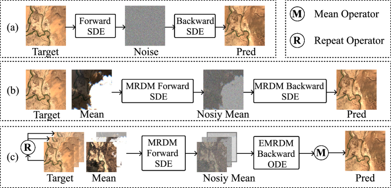
Figure 1: Comparison of EMRDM (c) with generative DMs (a) and MRDMs (b). Here, target is the cloudless image, pred is the CR prediction result, mean is the cloudy image, and noisy mean is the noisy cloudy image. The forward processes of (a), (b), and (c) generate diffused images approximated by noise (for DMs) and noisy mean (for EMRDM and MRDMs), respectively.

Satellite imagery, as a fundamental remote sensing product [yuan2020deep, zhu2017deep], enables diverse applications including environmental monitoring [vakalopoulou2015building], land cover classification [kussul2017deep], and agricultural monitoring [russwurm2017temporal]. However, cloud coverage severely affects the usability of satellite imagery. Data analysis for the Moderate Resolution Imaging Spectroradiometer (MODIS) on the Terra and Aqua satellites indicates that about 67% of the Earth’s surface experiences cloud coverage [king2013spatial]. Hence, cloud removal (CR) is a critical preliminary step in processing satellite imagery.

Recent advances in deep learning have driven the progress of CR [xiong2023sar-to-optical], with generative adversarial networks (GANs) [goodfellow2014generative] becoming a predominant approach. However, the effectiveness of GANs in CR is undermined by training instability [salimans2016improved] and mode collapse [bau2019seeing]. In comparison, diffusion models (DMs) [song2019generative, ho2020denoising, song2021scorebased] can overcome these limitations via enhanced training stability and output diversity, setting new benchmarks in image synthesis [dhariwal2021diffusion] and restoration [li2023diffusion]. Such advantages of DMs also extend to CR tasks [zou2024diffcr, zhao2023cloud, jing2023denoising, sui2024diffusion].

Existing diffusion-based CR methods typically employ vanilla DM frameworks that start the diffusion process from pure noise (Fig. 1 (a)). However, this is unnecessary as cloudy images contain substantial unexploited information. Even worse, noise-initiated generation lacks pixel-level consistency, inducing distortion [blau2018perception] in restored images due to poor fine-grained controllability. To resolve this, we propose the integration of mean-reverting diffusion models (MRDMs) [luo2023image] into CR. MRDMs start the diffusion process directly from noisy cloudy images (Fig. 1 (b)), intrinsically preserving structural fidelity through pixel-level consistency constraints. Specifically, the forward process progressively diffuses the target image by injecting noise while maintaining the cloudy image as the distribution mean, yielding a noisy cloudy image (noisy mean). Subsequent denoising in the backward process reconstructs the cloudless image (pred) while preserving structural consistency.

However, current MRDMs exhibit limitations due to their intricately coupled modules and opaque relationships among modules, impeding their application. Inspired by the successful designs of EDM [karras2022elucidating] in image generation, we conduct an in-depth analysis of the underlying mathematical principles of MRDMs to clarify the roles and interrelationships of modules within the MRDM framework. Based on these insights, we Elucidate the design space of MRDMs and propose a novel MRDM-based CR model, termed EMRDM. EMRDM offers a modular framework by reformulating the forward process through a stochastic differential equation (SDE) with simplified parameters and introducing an ordinary differential equation (ODE)-based backward process, as illustrated in Fig. 1 (c). The framework offers two critical advantages: (1) an elucidated and flexible design space enabling orthogonal module modifications, and (2) seamless compatibility with generative DMs. Leveraging the advantages of our framework, we further redesign key MRDM modules to boost CR performance, focusing on the following enhancements: (1) We restructure the denoiser via a preconditioning technique, inspired by image generation methods [karras2022elucidating, consistencymodel], to adaptively scale inputs and outputs of the denoising network according to noise levels. (2) We reorganize the training process and improve the sampling process. For practical sampling of CR results, we introduce novel deterministic and stochastic samplers based on the improved sampling process.

To achieve multi-temporal CR, we further develop a denoising network that processes arbitrary-length image sequences. Specifically, for $L$ sequential cloudy images, our architecture employs $L$ weight-sharing encoders and bottleneck modules, compresses temporal features through a novel attention block, and reconstructs outputs via a single decoder. The generated attention masks are preserved and upsampled to various resolutions, serving as adaptive weights to fuse temporal skip feature maps. The preconditioning and training methods are modified to accommodate multi-temporal scenarios through sequential input compatibility optimization. During sampling, to ensure temporal restoration consistency, we independently restore each temporal instance under mono-temporal conditions and aggregate results through a mean fusion operator (Fig. 1 (c)).

Our contributions are summarized as follows:

• We propose a novel CR model EMRDM that offers a modular framework with updatable modules and an elucidated design space.

• We develop a multi-temporal network with a temporal fusion method to denoise arbitrary-length image sequences.

• We restructure the denoiser via a preconditioning method, improve training and sampling processes, and propose novel stochastic and deterministic samplers.

• Experiments on mono-temporal and multi-temporal cases demonstrate the superior CR performance of EMRDM.

2 Related Work

Cloud Removal. CR methods are primarily divided into traditional methods [xu2019thin, xu2015thin, lin2012cloud] and deep learning-based methods, with the former offering better interpretability but generally inferior performance compared to data-driven methods. Deep learning-based methods are further categorized into mono-temporal [grohnfeldt2018conditional, enomoto2017filmy, bermudez2018sar, pan2020cloud, gao2020cloud, meraner2020cloud, xu2022glf, li2023transformer, ebel2023uncrtaints, zou2024diffcr] and multi-temporal [sarukkai2020cloud, huang2022ctgan, ebel2022sen12ms, ebel2023uncrtaints, zou2024diffcr, zhao2023cloud] paradigms based on single-image or sequential inputs. Mono-temporal methods commonly employ vanilla conditional GANs (cGANs) [goodfellow2014generative, mirza2014conditional] in early applications [enomoto2017filmy, bermudez2018sar, grohnfeldt2018conditional], with improvements including spatial attention [pan2020cloud] and transformer architectures [li2023transformer]. Alternative frameworks include DMs [zou2024diffcr] and non-generative models [meraner2020cloud, xu2022glf, ebel2023uncrtaints]. Multi-temporal strategies mainly use temporal cGAN [sarukkai2020cloud, huang2022ctgan], temporal fusion attention (e.g., L-TAE [garnot2020lightweight, garnot2021panoptic]) as in [ebel2023uncrtaints], and sequential DMs [zhao2023cloud]. CR methods are also classified as mono-modal [enomoto2017filmy, pan2020cloud, zou2024diffcr] or multi-modal, depending on the use of auxiliary modalities, including infrared (IR) and synthetic aperture radar (SAR) images. Multi-modal methods involve modality concatenation [bermudez2018sar, grohnfeldt2018conditional, meraner2020cloud, ebel2023uncrtaints, ebel2022sen12ms, sarukkai2020cloud, huang2022ctgan] and specialized fusion modules [gao2020cloud, xu2022glf, zhao2023cloud].

Diffusion Models. Recent advances in generative modeling have witnessed DMs [ho2020denoising, song2019generative, song2021scorebased] surpass GANs [dhariwal2021diffusion] in image synthesis. Notable improvements to DMs [rombach2022high, karras2022elucidating, peebles2023scalable, crowson2024scalable] have also been proposed, with EDM [karras2022elucidating] and HDiT [crowson2024scalable] most crucial to our work. EDM presents a framework that delineates the specific design decisions for DM components, while HDiT introduces an efficient hourglass diffusion transformer. Inspired by the success of DMs in image generation, extensive studies have investigated their applications in image restoration [li2023diffusion]. These methods can be categorized as supervised learning [saharia2022image, saharia2022palette, xia2023diffir, luo2023image, luo2023refusion, delbracio2023inversion, liu2024residual, liu2023I2SB, yue2024resshift, bansal2024cold] or zero-shot learning [Choi_2021_ICCV, lugmayr2022repaint, kawar2022denoising, wang2023zeroshot, song2023pseudoinverse]. In the first category, several methods focus on generating images directly from noiseless or noisy corrupted images, such as IR-SDE [luo2023image], InDI [delbracio2023inversion], ResShift [yue2024resshift], RDDM [liu2024residual], and I2SB [liu2023I2SB]. Considering that starting with pure noise is inefficient, IR-SDE, InDI, ResShift, and RDDM all integrate the corrupted image and noise within the diffusion process. We extend this paradigm and apply it to CR.

3 Methodology

As illustrated in Fig. 2, we introduce the EMRDM framework in Sec. 3.2, propose a novel multi-temporal denoising network in Sec. 3.3, restructure the denoiser by the preconditioning technique in Sec. 3.4, and present our redesigned training and sampling process in Sec. 3.5.

3.1 Preliminary

The forward process of DMs can be expressed as an SDE proposed by Song et al. (Eq. 5 in [song2021scorebased]), as follows:

$$\mathrm{d}\boldsymbol{x}=\boldsymbol{f}(\boldsymbol{x},t)\mathrm{d}t+g(t)\mathrm{d}\boldsymbol{\omega}_{t},$$ (1)

where $\boldsymbol{\omega}_{t}$ is a standard Brownian motion, $\boldsymbol{x}\in\mathbb{R}^{d}$ is an Itô process, $\boldsymbol{f}(\cdot,t):{\mathbb{R}}^{d}\rightarrow{\mathbb{R}}^{d}$ and $g(\cdot):{\mathbb{R}}\rightarrow{\mathbb{R}}$ are the drift and diffusion coefficients, respectively, and $d$ is the dimensionality of images. Song et al. further derive a reverse probability flow ODE (Eq. 13 in [song2021scorebased]) for sampling as

$$\mathrm{d}\boldsymbol{x}=\left[\boldsymbol{f}(\boldsymbol{x},t)-\frac{1}{2}{g(t)}^{2}\nabla_{\boldsymbol{x}}\log p_{t}(\boldsymbol{x})\right]\mathrm{d}t,$$ (2)

where $p_{t}(\boldsymbol{x})$ is the probability density function (pdf) of $\boldsymbol{x}$ at time $t$. The score function $\nabla_{\boldsymbol{x}}\log p_{t}(\boldsymbol{x})$ is predicted by a neural network. Therefore, the models proposed by [song2021scorebased], as well as our models, are score matching models.

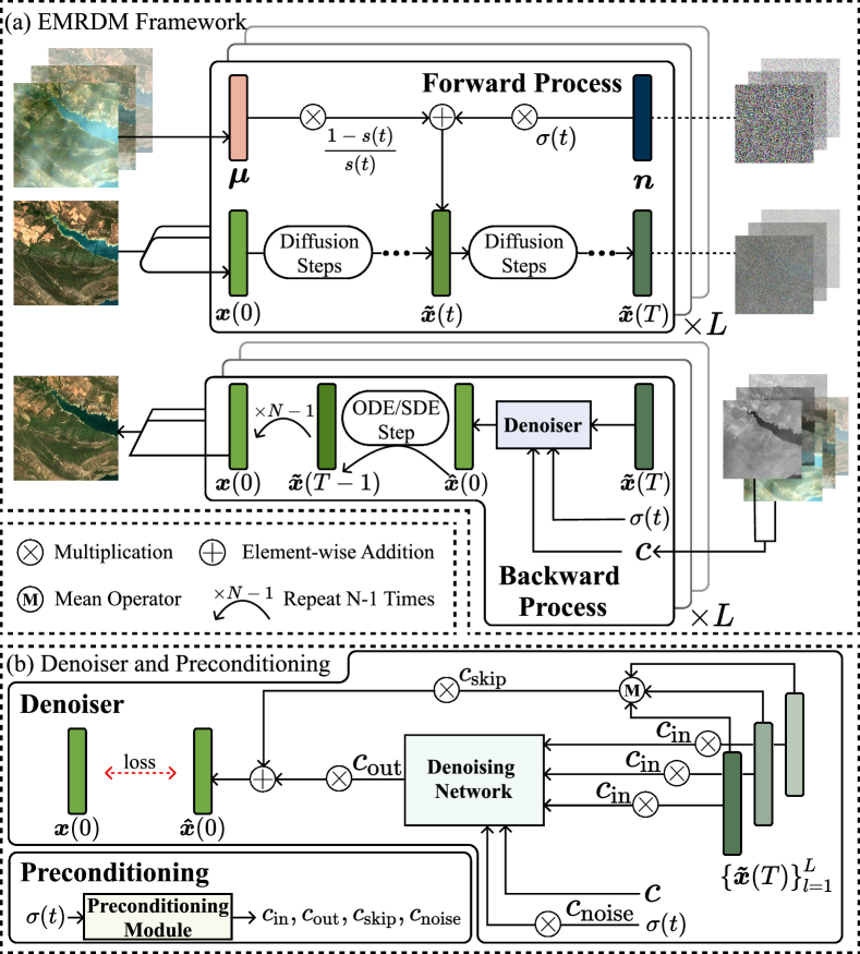
Figure 2: (a) The EMRDM framework comprises a forward process and a backward process that contains a denoiser. (b) The denoiser consists primarily of a denoising network, where the preconditioning module generates reparameterized factors $c_{\text{in}}\left(\sigma\right),c_{\text{out}}\left(\sigma\right),c_{\text{skip}}\left(\sigma\right),c_{\text{noise}}\left(\sigma\right)$ based on noise level $\sigma(t)$. We show the multi-temporal condition with the sequence length $L$.

3.2 The EMRDM Framework

We reformulate the forward process of MRDMs to construct a stochastic process $\{\boldsymbol{x}(t)\}_{t=0}^{T}$ that transforms a target image into its noisy cloudy counterpart. The new ODE-based backward process iteratively denoises the corrupted images.

Forward Process. We transform the SDE in Eq. 1 into

$$\mathrm{d}\boldsymbol{x}=f(t)(\boldsymbol{x}-\boldsymbol{\mu})\mathrm{d}t+g(t)\mathrm{d}\boldsymbol{\omega}_{t},$$ (3)

where $\boldsymbol{\mu}\in\mathbb{R}^{d}$ is the cloudy image, and the stochastic process $\boldsymbol{x}(t)$ is simplified to $\boldsymbol{x}$. According to [luo2023image], Eq. 3 can be viewed as a special case of Eq. 1 by defining $\boldsymbol{f}(\boldsymbol{x},t)=f(t)(\boldsymbol{x}-\boldsymbol{\mu})$. This setting yields a solution for the pdf of $\boldsymbol{x}(t)$ given $\boldsymbol{x}(0)$ and $\boldsymbol{\mu}$:

$$p_{0t}\big{(}\boldsymbol{x}(t)\mid\boldsymbol{x}(0),\boldsymbol{\mu}\big{)} ={s(t)}^{-d}\tilde{p}_{0t}\big{(}\boldsymbol{\tilde{x}}(t)\mid\boldsymbol{\tilde{x}}_{0}(t)\big{)},$$ (4)

$$\tilde{p}_{0t}\big{(}\boldsymbol{\tilde{x}}(t)\mid\boldsymbol{\tilde{x}}_{0}(t)\big{)} =\mathcal{N}\left(\cfrac{\boldsymbol{x}(t)}{s(t)};\boldsymbol{\tilde{x}}_{0}(t),{\sigma(t)}^{2}\boldsymbol{I}\right),$$ (5)

$$\boldsymbol{\tilde{x}}_{0}(t) =\boldsymbol{x}(0)+\frac{1-s(t)}{s(t)}\boldsymbol{\mu},$$ (6)

where $\mathcal{N}(\boldsymbol{x};\boldsymbol{m},\boldsymbol{\Sigma})$ denotes the Gaussian pdf evaluated at $\boldsymbol{x}$, with mean $\boldsymbol{m}$ and covariance $\boldsymbol{\Sigma}$. We define $\boldsymbol{\tilde{x}}(t)=\boldsymbol{x}(t)/s(t)$. The values of $s(t)$ and $\sigma(t)$ are as follows:

$$s(t)=\exp\left(\int_{0}^{t}{f(\xi)\mathrm{d}\xi}\right),\sigma(t)=\sqrt{\int_{0}^{t}{\frac{{g(\xi)}^{2}}{{s(\xi)}^{2}}}\mathrm{d}\xi}.$$ (7)

In our framework, $s(t)$ and $\sigma(t)$ are used instead of $f(t)$ and $g(t)$ for the design simplicity. By introducing the mean-adding term, i.e., $\frac{1-s(t)}{s(t)}\boldsymbol{\mu}$, in Eq. 6, the mean of $\boldsymbol{\tilde{x}}(t)$ approximately shifts to $\boldsymbol{\mu}$, unlike generative DMs with a final mean of zero. Hence, the SDE in Eq. 3 is named the mean-reverting SDE. Concretely:

• At $t=0$, it is obvious that $s(0)=1$ and $\sigma(0)=0$, ensuring $\boldsymbol{\tilde{x}}(0)=\boldsymbol{\tilde{x}}_{0}(0)=\boldsymbol{x}(0)$.

• At a large $t=T$, we require $\frac{1-s(T)}{s(T)}$ to be large enough to obscure $\boldsymbol{x}(0)$, ensuring that $\boldsymbol{\tilde{x}}(T)$ has a mean almost proportional to $\boldsymbol{\mu}$ and a standard variance equal to $\sigma(T)$.

With the techniques above, we establish a diffusion process that bridges the target image $\boldsymbol{x}(0)$ and the cloudy image $\boldsymbol{\mu}$ with noise $\boldsymbol{n}$, ensuring pixel-level fidelity in CR outputs. Notably, by omitting the mean-adding term (i.e., setting $s(t)=1$), the EMRDM framework reduces to the generative DM in [karras2022elucidating]. Hence, our framework expands the boundary of generative DMs.

See Sec. A.1 for derivations of the forward process.

Backward Process. We use $s(t)$ and $\sigma(t)$ to derive the backward ODE. Based on Eq. 2, we have

$$\mathrm{d}\boldsymbol{\tilde{x}}(t)=\left[-\cfrac{\dot{s}(t)}{{s(t)}^{2}}\boldsymbol{\mu}-\dot{\sigma}(t)\sigma(t)s_{\theta}\big{(}\boldsymbol{\tilde{x}}(t)\big{)}\right]\mathrm{d}t,$$ (8)

where $s_{\theta}\big{(}\boldsymbol{\tilde{x}}(t)\big{)}=\nabla_{\boldsymbol{\tilde{x}}(t)}\log p_{t}\big{(}\boldsymbol{\tilde{x}}(t)\big{)}$ is the score function [hyvarinen2005estimation], a vector field pointing to the higher density of data, with $\theta$ as its parameters. As $s_{\theta}\big{(}\boldsymbol{\tilde{x}}(t)\big{)}$ does not depend on the intractable form of $\log p_{t}\big{(}\boldsymbol{\tilde{x}}(t)\big{)}$ [hyvarinen2005estimation], it can be easily calculated. We use a denoiser function $D_{\theta}(\boldsymbol{x};\sigma;c)$ to predict it, with $\boldsymbol{x}$ as the image input, $\sigma$ as the noise level input, and $c$ as the conditioning input. By training $D_{\theta}$ as follows:

$$L\big{(}D_{\theta},\sigma(t)\big{)}= \mathbb{E}_{\boldsymbol{\tilde{x}}_{0}(t)\sim{p}_{\text{data}}}\mathbb{E}_{\boldsymbol{n}\sim\mathcal{N}\left(0,{\sigma(t)}^{2}\boldsymbol{I}\right)}$$ (9)

$${\|D_{\theta}\big{(}\boldsymbol{\tilde{x}}_{0}(t)+\boldsymbol{n};\sigma(t);c\big{)}-\boldsymbol{\tilde{x}}_{0}(0)\|}_{2}^{2},$$

with $p_{\text{data}}$ as the distribution of $\boldsymbol{\tilde{x}}_{0}(t)$, we can acquire

$$s_{\theta}\big{(}\boldsymbol{\tilde{x}}(t)\big{)}=\frac{D_{\theta}\big{(}\boldsymbol{\tilde{x}}(t);\sigma(t);c\big{)}+\frac{1-s(t)}{s(t)}\boldsymbol{\mu}-\boldsymbol{\tilde{x}}(t)}{{\sigma(t)}^{2}}.$$ (10)

Though it is common to directly use a neural network as the denoiser $D_{\theta}$, it is suboptimal for stable and effective training, as explained in Sec. 3.3. Hence, as shown in Fig. 2, we restructure $D_{\theta}$ by training a different network $F_{\theta}$ via the preconditioning technique. Sec. 3.3 provides details on $F_{\theta}$, while the relationship between $F_{\theta}$ and $D_{\theta}$ is discussed in Sec. 3.4. By substituting Eq. 10 into Eq. 8, we obtain

$$\mathrm{d}\boldsymbol{\tilde{x}}(t)={\Bigg{[}-\cfrac{\dot{s}(t)}{{s(t)}^{2}}\boldsymbol{\mu}-\cfrac{\dot{\sigma}(t)}{\sigma(t)}\times\Bigg{.}}$$ (11)

$${\Bigg{.}\left(D_{\theta}\big{(}\boldsymbol{\tilde{x}}(t);\sigma(t);c\big{)}+\cfrac{1-s(t)}{s(t)}\boldsymbol{\mu}-\boldsymbol{\tilde{x}}(t)\right)\Bigg{]}}\mathrm{d}t.$$

See Sec. A.2 for the proof of Eqs. 8, 9, 10 and 11. We redesign the samplers based on this ODE, detailed in Sec. 3.5. Generally, as depicted in Fig. 2 (a), at time $T$, the samplers iteratively use $D_{\theta}$ to estimate $\boldsymbol{x}(0)$. The output $\hat{\boldsymbol{x}}(0)$ is used in Eq. 11 to compute the next-step image $\boldsymbol{\tilde{x}}(T-1)$ for $N$ steps, ultimately restoring the image.

Choices of $s(t)$ and $\sigma(t)$. It is essential to ensure $\sigma(0)=0$ and $\lim_{t\rightarrow 0}\frac{1-s(t)}{s(t)}=0$. We adopt the linear choice $\sigma(t)=t$ according to [karras2022elucidating], and set $s(t)=\frac{1}{1+\alpha t}$, where $\alpha$ controls the mean reversion rate. Such settings yield a simpler SDE parameterization compared to prior MRDMs [luo2023image].

3.3 Multi-temporal Denoising Network

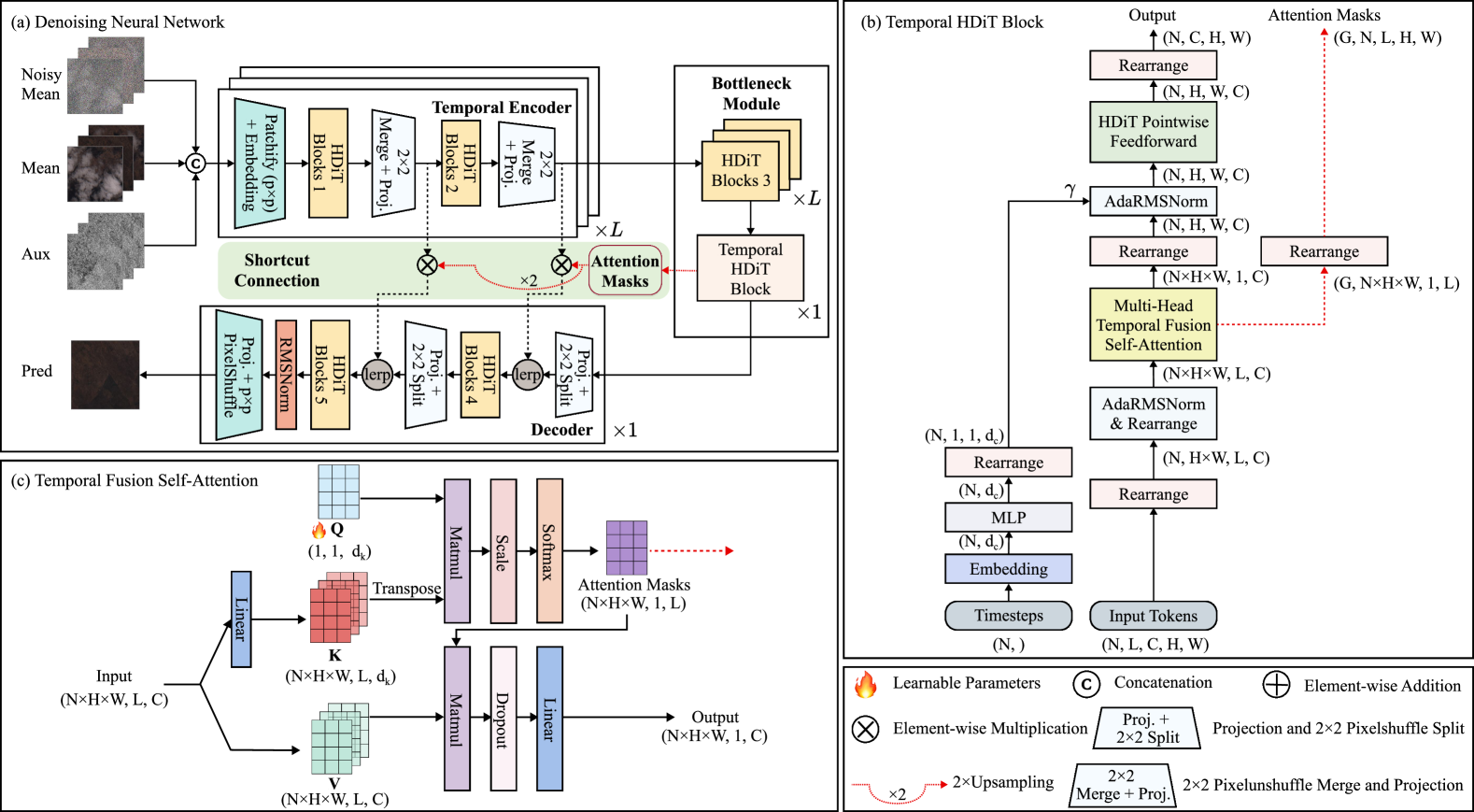
Figure 3: Illustration of the denoising network. (a) The network concurrently denoises sequences of noisy cloudy images (noisy mean), cloudy images (mean), and optional auxiliary modal images (aux) to generate results (pred). The notation $\times L$ indicates $L$ weight-sharing copies. (b) We extend the original HDiT Blocks to THDiT Blocks to integrate temporal information. (c) TFSA collapses the temporal dimension of inputs and generates the attention masks. For simplicity, we present a single-head scenario. Feature map dimensions are indicated below each block, where $N$ is the batch size, $H$ is the height, $W$ is the width, $L$ is the sequence length, $C$ is the channels of feature maps, $G$ is the number of heads, $d_{c}$ is the channels of condition vectors, and $d_{k}$ is the channels of query and key matrices.

Network Architecture. For mono-temporal CR, previous improvements to the denoising network [peebles2023scalable, crowson2024scalable, bao2023all] can be directly used, as it is orthogonal to other modules. We choose HDiT [crowson2024scalable] for effectiveness and efficiency. To adapt HDiT to CR tasks, we reset the input channels and remove the non-leaking augmentation [karras2020training] and classifier-free guidance [ho2021classifierfree], as they are unsuitable for restoration. Following [saharia2022palette], we concatenate the noisy cloudy image $\boldsymbol{\tilde{x}}_{0}(t)+n$ with the condition $c$. The condition includes cloudy images and optional auxiliary modal images (e.g., SAR or IR images).

To extend HDiT to multi-temporal CR tasks, we propose a new denoising network based on UTAE [garnot2021panoptic] to denoise sequential images. As shown in Fig. 3 (a), we retain the main architecture of HDiT and create $L$ weight-sharing copies of the encoder and middle HDiT blocks 3, while keeping the decoder unchanged. In the bottleneck module, we introduce a temporal HDiT block (THDiT), allowing sequential feature maps to be condensed into one map. Attention masks are generated from THDiT and used to collapse the temporal dimension of the skip feature maps per resolution:

$$o^{i}=\text{Concat}{\left[\sum_{l=1}^{L}{\text{bilinear}(a^{g}_{l},i)\odot e^{i,g}_{l}}\right]}_{g=1}^{G},$$ (12)

where $o^{i}$ is the output skipping feature map to the decoder at resolution level $i$, $a^{g}_{l}$ is the attention mask at head $g$ and time $l$, $e^{i,g}_{l}$ is the input feature map from the encoder at head $g$, time $l$ and resolution level $i$, $G$ is the number of heads, $\odot$ is the element-wise multiplication, and $\text{bilinear}(\cdot,i)$ indicates upsampling the map from the lowest resolution to level $i$.

Temporal HDiT Block. THDiT is modified from the original HDiT block. As shown in Fig. 3 (b), we replace spatial attention with our proposed temporal fusion self-attention (TFSA) to merge sequential feature maps and generate attention masks. We also introduce rearrangement layers to ensure that the feature maps have the correct shape before entering different blocks. As the temporal dimension collapses after TFSA, we remove the residual connection.

Temporal Fusion Self-Attention. As shown in Fig. 3 (c), TFSA adopts vanilla multi-head self-attention. Following L-TAE [garnot2020lightweight], we define query, key and value matrices as $\boldsymbol{Q}\in\mathbb{R}^{1\times d_{k}},\boldsymbol{K}=\boldsymbol{X}\boldsymbol{W}\in\mathbb{R}^{L\times d_{k}},\boldsymbol{V}=\boldsymbol{X}\in\mathbb{R}^{L\times C},$ respectively. Here, we consider a single-head scenario and omit the batch size dimension for simplicity. The feature map $\boldsymbol{X}$ has a sequence length of $L$ and $C$ channels. Both $\boldsymbol{Q}$ and $\boldsymbol{K}$ have $d_{k}$ channels. We use $\boldsymbol{X}$ as $\boldsymbol{V}$, and project it to $\boldsymbol{K}$ with weights $\boldsymbol{W}\in\mathbb{R}^{C\times d_{k}}$. $\boldsymbol{Q}$ is set as a learnable parameter and initialized from a normal distribution, with a sequence length of $1$ to condense the temporal information.

3.4 Preconditioning

In this section, we restructure the denoiser via the preconditioning technique to adaptively scale inputs and outputs according to noise variance $\sigma(t)$, focusing on multi-temporal CR, with the mono-temporal case covered by setting $L=1$. We use the superscript $l$ to represent the time point.

For training a network, it is advisable to maintain both inputs and outputs with unit variance [huang2023normalization, bishop1995neural], thus stabilizing and enhancing the training process. While directly training denoiser $D_{\theta}$ is not ideal for this purpose, we train a network $F_{\theta}$ instead via the preconditioning technique to scale inputs and outputs to unit variance, following EDM [karras2022elucidating]. As shown in Fig. 2 (b), the relation between $D_{\theta}$ and $F_{\theta}$ is:

$$D_{\theta}\left(\{\boldsymbol{\tilde{x}}^{l}\}_{l=1}^{L};\sigma;c\right)=\text{mean}\left(\{c_{\text{skip}}\left(\sigma\right)\boldsymbol{\tilde{x}}^{l}\}_{l=1}^{L}\right)$$ (13)

$$+c_{\text{out}}\left(\sigma\right)F_{\theta}\left(\{c_{\text{in}}\left(\sigma\right)\boldsymbol{\tilde{x}}^{l}\}_{l=1}^{L};c_{\text{noise}}\left(\sigma\right);c\right),$$

where $\sigma(t)$ is simplified to $\sigma$ and $\boldsymbol{\tilde{x}}(t)^{l}$ is simplified to $\boldsymbol{\tilde{x}}^{l}$. The output shape of $F_{\theta}$ differs from the input shape, which requires a mean operator to reduce the temporal dimension of $\{c_{\text{skip}}\left(\sigma\right)\boldsymbol{\tilde{x}}^{l}\}_{l=1}^{L}$. As our network can process sequential images, $\{c_{\text{in}}\left(\sigma\right)\boldsymbol{\tilde{x}}^{l}\}_{l=1}^{L}$ does not need the mean operator. To ensure that inputs and targets have unit variance, we introduce four factors $c_{\text{in}}\left(\sigma\right)$, $c_{\text{skip}}\left(\sigma\right)$, $c_{\text{out}}\left(\sigma\right)$ and $c_{\text{noise}}\left(\sigma\right)$ to scale the inputs and outputs governed by four hyperparameters: $\sigma_{\text{data}}$ (the variance of target images), $\sigma_{\text{mu}}$ (the variance of cloudy images), $\sigma_{\text{cov}}$ (the covariance between target and cloudy images), and $L$ (sequence length):

$$c_{\text{in}}(\sigma) =\frac{1}{\sqrt{\sigma_{\text{data}}^{2}+k^{2}\sigma_{\text{mu}}^{2}+\sigma^{2}+2k\sigma_{\text{cov}}}},$$ (14)

$$c_{\text{skip}}(\sigma) =\frac{\sigma_{\text{data}}^{2}+k\sigma_{\text{cov}}}{\sigma_{\text{data}}^{2}+k^{2}\sigma_{\text{mu}}^{2}+\frac{\sigma^{2}}{L}+2k\sigma_{\text{cov}}},$$ (15)

$$c_{\text{out}}(\sigma) =\sqrt{\frac{k^{2}\sigma_{\text{mu}}^{2}\sigma_{\text{data}}^{2}+\frac{\sigma^{2}}{L}\sigma_{\text{data}}^{2}-k^{2}\sigma_{\text{cov}}^{2}}{\sigma_{\text{data}}^{2}+k^{2}\sigma_{\text{mu}}^{2}+\frac{\sigma^{2}}{L}+2k\sigma_{\text{cov}}}},$$ (16)

$$c_{\text{noise}}(\sigma) =\frac{1}{4}\ln(\sigma),$$ (17)

where $k$ represents $k(t)$, and $k(t)=\frac{1-s(t)}{s(t)}$. Notably, setting $\sigma_{\text{mu}}=\sigma_{\text{cov}}=0$ reverts Eqs. 14, 16, 15 and 17 to their original form in EDM. See Sec. A.3 for derivations.

3.5 Training and Sampling

This section details the training and sampling processes under the multi-temporal scenario, with the mono-temporal case covered by setting $L=1$.

Training. The training process is detailed in Algorithm 1. We retain the training distribution of $\sigma$ in [karras2022elucidating] (line 2). Sequential images are then independently perturbed (lines 4 to 6) and denoised jointly (line 7). We further introduce a parameter $\lambda\left(\sigma\right)$ to adjust the loss function at different noise levels during training (line 9):

$$\mathbb{E}_{\sigma,\boldsymbol{x}(0),\boldsymbol{n}}\left[{\lambda\left\|D_{\theta}\left(\{\boldsymbol{\tilde{x}}_{0}^{l}+\boldsymbol{n}\}_{l=1}^{L};\sigma,c\right)-\boldsymbol{x}(0)\right\|}_{2}^{2}\right],$$ (18)

where $\lambda$ and $\boldsymbol{\tilde{x}}_{0}^{l}$ represent $\lambda\left(\sigma\right)$ and $\boldsymbol{\tilde{x}}_{0}^{l}(t)$, respectively. We set $\lambda(\sigma)=\frac{1}{{c_{\text{out}}(\sigma)}^{2}}$, in accordance with EDM [karras2022elucidating].

Sampling. As outlined in Algorithm 2, we design a stochastic sampler. It begins with the sequential sampling of noisy images (lines 2 to 3). Within the sampling loop, $\gamma_{i}$ is computed (line 5) to perturb the time $t_{i}$ to a higher noise level $\hat{t}_{i}$ (line 6). Updated samples $\hat{\boldsymbol{x}}_{i}^{l}$ at noise level $\hat{t}_{i}$ are obtained:

$$\hat{\boldsymbol{x}}_{i}^{l}=\boldsymbol{x}_{i}^{l}+\left(k(\hat{t}_{i})-k(t_{i})\right)\boldsymbol{\mu}^{l}+\sqrt{\sigma(\hat{t}_{i})^{2}-\sigma(t_{i})^{2}}\boldsymbol{\epsilon}_{i}^{l},$$ (19)

where $\boldsymbol{\epsilon}_{i}^{l}$ denotes Gaussian noise. The Euler step (lines 10 to 12) based on Eq. 11 computes the next sample $\boldsymbol{x}_{i+1}^{l}$ for each $l$. The loop ends with a mean operator to collapse the temporal dimension of $\{\boldsymbol{x}_{N}^{l}\}_{l=1}^{L}$. The method includes following hyperparameters: $N$, $S_{\text{churn}}$, $S_{\text{tmin}}$, $S_{\text{tmax}}$ and $S_{\text{noise}}$, as in EDM. $N$ is the number of sample steps. $S_{\text{churn}}$, $S_{\text{tmin}}$ and $S_{\text{tmax}}$ control $\gamma_{i}$, while $S_{\text{noise}}$ regulates the variance of $\boldsymbol{\epsilon}_{i}^{l}$. The stochastic sampler becomes deterministic when setting $S_{\text{churn}}=0$. In addition, we should set a range for $\sigma$ when sampling. In other words, $\sigma(t_{N-1})=\sigma_{\text{max}}$ and $\sigma(t_{0})=\sigma_{\text{min}}$. Both $\sigma_{\text{max}}$ and $\sigma_{\text{min}}$ are also hyperparameters. The intermediate $\sigma$ values are interpolated following EDM (Eq. 5 in [karras2022elucidating]). See Sec. A.4 for more details.

Algorithm 1 Our training step with $s(t)={1}/{\left(1+\alpha t\right)}$ and $\sigma(t)=t$.

1:procedure TrainStep($\boldsymbol{x}(0),{\{\boldsymbol{\mu}^{l}\}}_{l=1}^{L},c,D_{\theta}$)

2:  sample $\ln(\sigma)\sim\mathcal{N}(P_{\text{mean}},P_{\text{std}}^{2})$

3:  $\sigma\leftarrow\exp\big{(}\ln(\sigma)\big{)}$

4:  for $l\in\{1,2,\cdots,L\}$ do

5:   sample $\boldsymbol{n}^{l}\sim\mathcal{N}(0,\boldsymbol{I})$

6:   $\boldsymbol{\tilde{x}}_{0}^{l}(t)\leftarrow\boldsymbol{x}(0)+\alpha\sigma\boldsymbol{\mu}^{l},\boldsymbol{\tilde{x}}^{l}(t)\leftarrow\boldsymbol{\tilde{x}}_{0}^{l}(t)+\sigma\boldsymbol{n}^{l}$   

7:  $\hat{\boldsymbol{x}}(0)\leftarrow D_{\theta}\left(\{\boldsymbol{\tilde{x}}^{l}(t)\}_{l=1}^{L};\sigma;c\right)$ $\triangleright$ Eq. 13

8:  Take gradient descent step on

9:   $\nabla_{\boldsymbol{x}}\mathbb{E}_{\sigma,\boldsymbol{x}(0),\boldsymbol{n}}\left[{\lambda(\sigma)\|\hat{\boldsymbol{x}}(0)-\boldsymbol{x}(0)\|}_{2}^{2}\right]$ $\triangleright$ Eq. 18

Algorithm 2 Our stochastic sampler with $s(t)={1}/{\left(1+\alpha t\right)}$ and $\sigma(t)=t$.

1:procedure StochasticSampler(${\{\boldsymbol{\mu}^{l}\}}_{l=1}^{L},c,D_{\theta}$)

2:  for $l\in\{1,2,\cdots,L\}$ do

3:   sample $\boldsymbol{x}_{0}^{l}\sim\mathcal{N}(\alpha\sigma\boldsymbol{\mu}^{l},\sigma^{2}\boldsymbol{I})$   

4:  for $i\in\{0,1,\cdots,N-1\}$ do

5:   $\gamma_{i}\leftarrow S_{\text{churn}}/N$ if $t_{i}\in[S_{\text{tmin}},S_{\text{tmax}}]$ else 0

6:   $\hat{t}_{i}\leftarrow t_{i}+\gamma_{i}t_{i}$

7:   for $l\in\{1,2,\cdots,L\}$ do

8:     sample $\boldsymbol{\epsilon}_{i}^{l}\in\mathcal{N}\left(0,S^{2}_{\text{noise}}\boldsymbol{I}\right)$

9:     $\hat{\boldsymbol{x}}_{i}^{l}\leftarrow\boldsymbol{x}_{i}^{l}+\alpha(\hat{t}_{i}-t_{i})\boldsymbol{\mu}^{l}+\sqrt{\hat{t}_{i}^{2}-t_{i}^{2}}\boldsymbol{\epsilon}_{i}^{l}$ $\triangleright$ Eq. 19    

10:   for $l\in\{1,2,\cdots,L\}$ do

11:     $\boldsymbol{d}_{i}^{l}\leftarrow\left({\hat{\boldsymbol{x}}_{i}^{l}-D_{\theta}\big{(}\{\hat{\boldsymbol{x}}_{i}^{l}\}_{l=1}^{L};\sigma;c\big{)}}\right)/{\hat{t}_{i}}$ $\triangleright$ Eq. 11

12:     $\boldsymbol{x}_{i+1}^{l}\leftarrow\hat{\boldsymbol{x}}_{i}^{l}+(t_{i+1}-\hat{t}_{i})\boldsymbol{d}_{i}^{l}$      

13:  $\boldsymbol{x}_{N}\leftarrow\text{mean}\left(\{\boldsymbol{x}_{N}^{l}\}_{l=1}^{L}\right)$

14:  return $\boldsymbol{x}_{N}$

4 Performance Evaluation

Table 1: Quantitative results on (a) CUHK-CR1, (b) CUHK-CR2, (c) SEN12MS-CR, and (d) Sen2_MTC_New datasets. The metrics align with those used in prior studies on these datasets. The symbols $\uparrow$/$\downarrow$ indicate that higher/lower values correspond to better performance. The best results are highlighted in red bold underline, while the second-best results are marked in blue bold. Dashed lines separate diffusion-based approaches from others.

Method	(a) CUHK-CR1			(b) CUHK-CR2
	PSNR$\uparrow$	SSIM$\uparrow$	LPIPS$\downarrow$	PSNR$\uparrow$	SSIM$\uparrow$	LPIPS$\downarrow$
SpA-GAN [pan2020cloud]	20.999	0.5162	0.0830	19.680	0.3952	0.1201
AMGAN-CR [xu2022attention]	20.867	0.4986	0.1075	20.172	0.4900	0.093
CVAE [ding2022uncertainty]	24.252	0.7252	0.1075	22.631	0.6302	0.0489
MemoryNet [zhang2023memory]	26.073	0.7741	0.0315	24.224	0.6838	0.0403
MSDA-CR [yu2022cloud]	25.435	0.7483	0.0374	23.755	0.6661	0.0433
DE-MemoryNet [sui2024diffusion]	26.183	0.7746	0.0290	24.348	0.6843	0.0369
DE-MSDA [sui2024diffusion]	25.739	0.7592	0.0321	23.968	0.6737	0.0372
Ours (EMRDM)	27.281	0.8007	0.0218	24.594	0.6951	0.0301

(c) SEN12MS-CR	PSNR$\uparrow$	SSIM$\uparrow$	MAE$\downarrow$	SAM$\downarrow$
McGAN [enomoto2017filmy]	25.14	0.744	0.048	15.676
SAR-Opt-cGAN [grohnfeldt2018conditional]	25.59	0.764	0.043	15.494
SAR2OPT [bermudez2018sar]	25.87	0.793	0.042	14.788
SpA GAN [pan2020cloud]	24.78	0.754	0.045	18.085
Simulation-Fusion GAN [gao2020cloud]	24.73	0.701	0.045	16.633
DSen2-CR [meraner2020cloud]	27.76	0.874	0.031	09.472
GLF-CR [xu2022glf]	28.64	0.885	0.028	08.981
UnCRtainTS L2 [ebel2023uncrtaints]	28.90	0.880	0.027	08.320
ACA-Net [huang2024attentive]	29.78	0.896	0.025	07.770
DiffCR [zou2024diffcr]	31.77	0.902	0.019	05.821
Ours (EMRDM)	32.14	0.924	0.018	05.267

(d) Sen2_MTC_New	PSNR$\uparrow$	SSIM$\uparrow$	LPIPS$\downarrow$
McGAN [enomoto2017filmy]	17.448	0.513	0.447
Pix2Pix [isola2017image-to-image]	16.985	0.455	0.535
AE [sintarasirikulchai2018a]	15.100	0.441	0.602
STNet [chen2020thick]	16.206	0.427	0.503
DSen2-CR [meraner2020cloud]	16.827	0.534	0.446
STGAN [sarukkai2020cloud]	18.152	0.587	0.513
CTGAN [huang2022ctgan]	18.308	0.609	0.384
SEN12MS-CR-TS Net  [ebel2022sen12ms]	18.585	0.615	0.342
PMAA [zou2023pmaa]	18.369	0.614	0.392
UnCRtainTS [ebel2023uncrtaints]	18.770	0.631	0.333
DDPM-CR [jing2023denoising]	18.742	0.614	0.329
DiffCR [zou2024diffcr]	19.150	0.671	0.291
Ours (EMRDM)	20.067	0.709	0.255

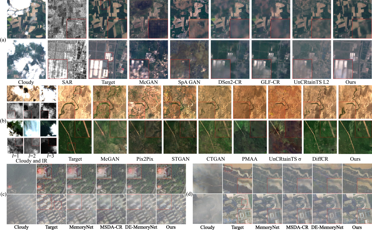
Figure 4: (a) SEN12MS-CR dataset results: RGB channels for optical imagery (linearly enhanced for visualization) and VV channel for SAR imagery. GLF-CR results are obtained by combining four separately processed subimages as it processes $128\times 128$ images ($256\times 256$ for others). (b) Sen2_MTC_New dataset results. (c,d) RGB channel results on CUHK-CR1 and CUHK-CR2 datasets, respectively.

4.1 Implementation Details

We conduct experiments on four datasets: CUHK-CR1 [sui2024diffusion], CUHK-CR2 [sui2024diffusion] and SEN12MS-CR [ebel2020multisensor] for mono-temporal CR tasks; and Sen2_MTC_New [huang2022ctgan] for multi-temporal CR tasks with $L=3$. MAE, PSNR, SSIM, SAM, and LPIPS are used as evaluation metrics. We move more implementation details to Sec. C.1.

4.2 Performance Comparison

All quantitative results are illustrated in Tab. 1 using the optimal configuration for each model for a fair comparison. EMRDM surpasses all previous methods across all datasets and metrics, demonstrating its superiority. On the SEN12MS-CR dataset containing multi-spectral optical and auxiliary SAR images, EMRDM achieves significant improvements over existing methods. This validates its capability to exploit SAR’s all-weather imaging characteristics and effectively process multi-spectral inputs. On the CUHK-CR1, CUHK-CR2, and Sen2_MTC_New datasets that mainly consist of RGB channels, EMRDM attains remarkable results across perceptual quality (LPIPS) and structural consistency metrics (SSIM, PSNR). Notably, it maintains performance superiority on the CUHK-CR1/CR2 datasets without auxiliary modalities, demonstrating robust CR capabilities with limited information. EMRDM further exhibits strong multi-temporal processing capability, as evidenced by leading metrics on the Sen2_MTC_New dataset. The visual results in Fig. 4 further prove the superior CR quality of EMRDM. In particular, when the input images are heavily cloud-covered, our model restores better textures, crucial for subsequent tasks after CR.

4.3 Ablation Study& Parameter Effect

Table 2: We conducted an ablation study on the Sen2_MTC_New dataset to evaluate our method by incrementally adding modules.

Training configuration	PSNR$\uparrow$	SSIM$\uparrow$	MAE$\downarrow$	SAM$\downarrow$	LPIPS$\downarrow$
a Baseline ($s(t)=1$)	12.81	0.342	0.204	13.005	0.718
b + Corrupted images	18.26	0.649	0.109	06.526	0.311
c + IR images	19.31	0.677	0.095	06.547	0.279
d + Our MRDM framework	19.52	0.679	0.092	06.551	0.278
e + Our preconditioning	19.47	0.693	0.093	06.390	0.267

Effects of Modules. We conduct ablation studies on key modules, as outlined in Tab. 2, using models trained for 500 epochs with a deterministic sampler, setting $N=5$, $\sigma_{\text{data}}=1.0$, $\sigma_{\text{min}}=0.001$ and $\sigma_{\text{max}}=100$ for a fair comparison. The baseline (config A) sets $s(t)=1$, reducing our method to generative DMs, with only noise images as inputs. Config B and C incorporate cloudy and IR images, respectively. The results demonstrate their essential roles as conditioning inputs. Config D verifies the effectiveness of the EMRDM framework in Sec. 3.2 with $s(t)=\frac{1}{1+t}$ and $\sigma_{\text{mu}}=\sigma_{\text{cov}}=0$. Incorporating preconditioning techniques proposed in Sec. 3.4 in config E, with $\sigma_{\text{mu}}=1.0$, $\sigma_{\text{cov}}=0.9$, results in improved performance.

Table 3: Hyperparameter analysis on the Sen2_MTC_New dataset.

Configurations				Metrics
$\alpha$	$\sigma_{\text{max}}$	$N$	PSNR$\uparrow$	SSIM$\uparrow$	MAE$\downarrow$	SAM$\downarrow$	LPIPS$\downarrow$
0.2	100.0	5	19.34	0.692	0.095	6.306	0.269
0.5			19.14	0.675	0.097	6.580	0.283
0.8			19.90	0.689	0.088	6.249	0.260
1.0			19.44	0.688	0.091	6.367	0.273
2.0			19.77	0.704	0.087	5.922	0.262
3.0			20.00	0.708	0.084	5.710	0.255
4.0			19.76	0.695	0.087	5.821	0.263
3.0	40	5	19.58	0.701	0.087	5.764	0.260
	60		19.88	0.706	0.085	5.733	0.257
	80		19.96	0.707	0.084	5.726	0.256
	100		20.00	0.708	0.084	5.710	0.255
	150		20.03	0.707	0.085	5.730	0.256
	200		20.03	0.707	0.085	5.723	0.256
	300		20.02	0.705	0.086	5.728	0.257
3.0	100	4	19.98	0.702	0.085	5.744	0.259
		5	20.00	0.708	0.084	5.710	0.255
		6	19.97	0.705	0.084	5.710	0.257
		8	19.89	0.700	0.085	5.695	0.257
		10	19.89	0.700	0.085	5.695	0.257
		15	19.55	0.672	0.088	5.715	0.261
		50	19.19	0.641	0.091	5.857	0.270

Effects of $\alpha$, $\sigma_{\text{max}}$ and $N$. Tab. 3 presents the results while varying key parameters. Each model is trained for 500 epochs, with $\sigma_{\text{data}}=\sigma_{\text{mu}}=1.0$ and $\sigma_{\text{cov}}=0.9$. We use a deterministic sampler with $\sigma_{\text{min}}=0.001$. For $\alpha$, which controls the ratio of $\boldsymbol{\mu}$ and $\boldsymbol{n}$ in the forward process, it yields the optimal results across all metrics when set to $3$. For $\sigma_{\text{max}}$, the results show that a moderate value (e.g., 100) produces almost all the best metrics. For $N$, surprisingly, contrary to the expectations in generative DMs, a large $N$ yields poor results, while using only five steps delivers superior results across most metrics. This finding aligns with [yue2024resshift].

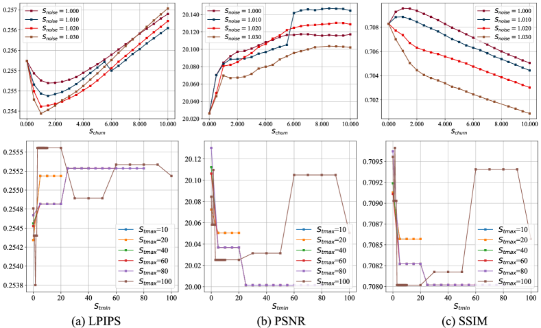
Figure 5: Analysis of our samplers on the Sen2_MTC_New dataset. When $S_{\text{churn}}=0$, the sampler reduces to be deterministic. The upper row shows the effects of $S_{\text{churn}}$ and $S_{\text{noise}}$ by fixing $S_{\text{tmin}}=0$ and $S_{\text{tmax}}\geq 100$. The lower row examines the effects of $S_{\text{tmin}}$ and $S_{\text{tmax}}$ with fixed $S_{\text{churn}}=1$ and $S_{\text{noise}}=1$. Note that $S_{\text{tmin}}>=S_{\text{tmax}}$ is excluded as this leads to a deterministic sampler.

Effect of Samplers. We examine our samplers in Fig. 5 using the $\alpha=3.0$ configuration in Tab. 3, and setting $\sigma_{\text{min}}=0.001$, $\sigma_{\text{max}}=100$, and $N=5$. According to the upper row of Fig. 5, the stochastic sampler consistently outperforms the deterministic one in PSNR, with $S_{\text{noise}}\in[1.000,1.020]$ and $S_{\text{churn}}\geq 6.0$ achieving superior scores. However, high $S_{\text{churn}}$ can negatively affect LPIPS and SSIM. While LPIPS is relatively insensitive to $S_{\text{noise}}$, SSIM declines at higher $S_{\text{noise}}$. We suggest using $S_{\text{noise}}\approx 1.000$ and $S_{\text{churn}}\approx 1.0$ for balanced metric performance. According to the lower row of Fig. 5, the optimal results are achieved across all metrics when $S_{\text{tmin}}\approx 0$. Generally, $S_{\text{tmax}}$ should be relatively large, such as 80 and 100.

Table 4: Analysis of $L$ on the Sen2_MTC_New dataset.

Sequence Length	PSNR$\uparrow$	SSIM$\uparrow$	MAE$\downarrow$	SAM$\downarrow$	LPIPS$\downarrow$
$L=1$	16.09	0.493	0.146	7.773	0.440
$L=2$	18.10	0.623	0.106	7.313	0.344
$L=3$	20.07	0.709	0.084	5.670	0.255

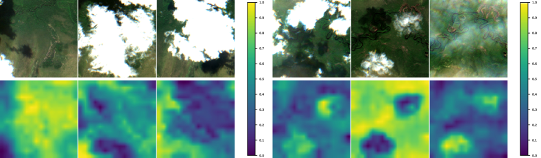
Figure 6: Visualizations of attention masks and their corresponding cloudy images from two cases on the Sen2_MTC_New dataset. Each mask at different time points is normalized to the range $[0,1]$ and upsampled using bilinear interpolation to match the size of the cloudy images for clarity. The left panel shows a case from head $0$, while the right panel displays a case from head $15$.

Effect of the Network. We analyze the impact of $L$ on our network (see Tab. 4), with models trained using the $\alpha=3.0$ configuration in Tab. 3 and evaluated via a deterministic sampler ($\sigma_{\text{min}}=0.001$, $\sigma_{\text{max}}=100$, and $N=5$). Increasing $L$ consistently boosts performance across all metrics, highlighting the benefits of multi-temporal inputs and our network’s ability to process them. Fig. 6 visualizes TFSA attention masks, with high attention scores for cloudless regions and low scores for cloudy ones. Regions occluded by clouds, characterized by low attention scores, correspondingly exhibit elevated scores in cloudless temporal counterparts. This validates TFSA’s capacity to compensate for corrupted information by integrating information from spatially equivalent regions across the temporal dimension.

5 Conclusion

We propose a novel MRDM-based CR model named EMRDM. It offers a modular framework with updatable modules and an elucidated design space. With this advantage, we redesign core MRDM modules to boost CR performance, including restructuring the denoiser via a preconditioning technique and improving training and sampling processes. To achieve multi-temporal CR, a new network is devised to process sequential images in parallel. These improvements enable EMRDM to achieve superior results on mono-temporal and multi-temporal CR benchmarks.

6 Acknowledgments

This work was supported in part by National Natural Science Foundation of China (No. 62202336, No. 62172300, No. 62372326), and the Fundamental Research Funds for the Central Universities (No. 2024-4-YB-03).

Supplementary Material

Appendix A Derivation of formulas

A.1 Forward Process

The forward process (i.e., diffusion process) is defined as the SDE in Eq. 3. The goal of this section is to derive the form of $p_{0t}\big{(}\boldsymbol{x}(t)\mid\boldsymbol{x}(0),\boldsymbol{\mu}\big{)}$, which is also called the perturbation kernel. We can rewrite the form of Eq. 3 into:

$$\mathrm{d}\boldsymbol{x}=-f(t)(\boldsymbol{\mu}-\boldsymbol{x})\mathrm{d}t+g(t)\mathrm{d}\boldsymbol{\omega}_{t},$$ (20)

whose solution has already been solved in IR-SDE (Eq. (6) in [luo2023image]), as

$$p_{0t}\big{(}\boldsymbol{x}(t)\mid\boldsymbol{x}(0),\boldsymbol{\mu}\big{)} =\mathcal{N}\big{(}\boldsymbol{x}(t);\boldsymbol{m}_{t},v_{t}\boldsymbol{I}\big{)},$$ (21)

$$\boldsymbol{m}_{t}=\boldsymbol{\mu}+\big{(}\boldsymbol{x}(0)-\boldsymbol{\mu}\big{)}e^{-\bar{\theta}_{0:t}} ,v_{t}=\int_{0}^{t}{{g(\xi)}^{2}e^{-2\bar{\theta}_{\xi:t}}}{\mathrm{d}\xi},$$ (22)

where $\bar{\theta}_{s:t}=\int_{s}^{t}{-f(\xi)}{\mathrm{d}\xi}$. Thus,

$$\boldsymbol{m}_{t} =\boldsymbol{\mu}+\big{(}\boldsymbol{x}(0)-\boldsymbol{\mu}\big{)}\exp\left(-\int_{0}^{t}{-f(\xi)}{\mathrm{d}\xi}\right)=\boldsymbol{\mu}+\big{(}\boldsymbol{x}(0)-\boldsymbol{\mu}\big{)}s(t),$$ (23)

$$v(t) =\int_{0}^{t}{{g(\xi)}^{2}\exp\left(-2\int_{\xi}^{t}-f(z)\mathrm{d}z\right)}{\mathrm{d}\xi}=\int_{0}^{t}{\left[g(\xi)\exp\left(\int_{\xi}^{t}{f(z)\mathrm{d}z}\right)\right]}^{2}{\mathrm{d}\xi}$$ (24)

$$=\int_{0}^{t}{\left[g(\xi)\exp\left(\int_{0}^{t}{f(z)\mathrm{d}z}-\int_{0}^{\xi}{f(z)\mathrm{d}z}\right)\right]}^{2}{\mathrm{d}\xi}=\int_{0}^{t}{\left[{\left(\cfrac{g(\xi)}{\exp\left(\int_{0}^{\xi}{f(z)\mathrm{d}z}\right)}\right)}^{2}\exp\left(2\int_{0}^{t}f(z)\mathrm{d}z\right)\right]}{\mathrm{d}\xi}$$ (25)

$$=\exp\left(2\int_{0}^{t}f(z)\mathrm{d}z\right)\int_{0}^{t}{{\left(\cfrac{g(\xi)}{s(\xi)}\right)}^{2}}{\mathrm{d}\xi}={s(t)}^{2}\sigma(t)^{2},$$ (26)

where $s(t)$ and $\sigma(t)$ is detailed in Eq. 7. Hence, the perturbation kernel can be rewritten as:

$$p_{0t}\big{(}\boldsymbol{x}(t)\mid\boldsymbol{x}(0),\boldsymbol{\mu}\big{)} =\mathcal{N}\left(\boldsymbol{x}(t);\boldsymbol{\mu}+s(t)\left(\boldsymbol{x}\left(0\right)-\boldsymbol{\mu}\right),s(t)^{2}\sigma(t)^{2}\boldsymbol{I}\right)$$ (27)

$$=s(t)^{-d}\mathcal{N}\left(\cfrac{\boldsymbol{x}(t)}{s(t)};\boldsymbol{x}(0)+\cfrac{1-s(t)}{s(t)}\boldsymbol{\mu},\sigma(t)^{2}\boldsymbol{I}\right)$$ (28)

$$=s(t)^{-d}\tilde{p}_{0t}\left(\boldsymbol{\tilde{x}}(t)\mid\boldsymbol{\tilde{x}}_{0}(t)\right),$$ (29)

where $d$ is the dimension of $\boldsymbol{x}$, $\boldsymbol{\tilde{x}}(t)$ is equal to $\cfrac{\boldsymbol{x}(t)}{s(t)}$, and $\boldsymbol{\tilde{x}}_{0}(t)$ along with $\tilde{p}_{0t}$ is defined in Eqs. 5 and 6. Eq. 29 is the same as Eq. 4.

A.2 Backward Process

As we have mentioned in Sec. 3.1, our forward SDE in Eq. 3 can be viewed as a special case of Eq. 1 proposed by [song2021scorebased], by defining $\boldsymbol{f}(x,t)=f(t)(\boldsymbol{x}-\boldsymbol{\mu})$. Thus, the backward ODE can also be seen as a special case of Eq. 2. By substituting the relationship between $\boldsymbol{f}(x,t)$ and $f(t)$ into Eq. 2, we can acquire:

$$\mathrm{d}\boldsymbol{x}=\left[f(t)(\boldsymbol{x}-\boldsymbol{\mu})-\frac{1}{2}{g(t)}^{2}\nabla_{\boldsymbol{x}}\log p_{t}(\boldsymbol{x})\right]\mathrm{d}t,$$ (30)

where we simplify $\boldsymbol{x}(t)$ to $\boldsymbol{x}$. According to Eq. 7, we can derive the relationship between $s(t)$, $\sigma(t)$ and $f(t)$,$g(t)$. This has already been demonstrated in the Eqs. (28) and (34) in [karras2022elucidating], which is

$$f(t)=\cfrac{\dot{s}(t)}{s(t)},g(t)=s(t)\sqrt{2\dot{\sigma}(t)\sigma(t)},$$ (31)

where $\dot{s}(t)$ and $\dot{\sigma}(t)$ are the derivatives of $s(t)$ and $\sigma(t)$, respectively. We can rewrite the form of Eq. 30 by substituting Eq. 31 into it:

$$\mathrm{d}\boldsymbol{x}=\left[\cfrac{\dot{s}(t)}{s(t)}(\boldsymbol{x}-\boldsymbol{\mu})-s(t)^{2}\dot{\sigma}(t)\sigma(t)\nabla_{\boldsymbol{x}}\log p_{t}(\boldsymbol{x})\right]\mathrm{d}t.$$ (32)

Since we define $\boldsymbol{\tilde{x}}(t)=\cfrac{\boldsymbol{x}(t)}{s(t)}$. We can obtain

$$\boldsymbol{x}(t)=s(t)\boldsymbol{\tilde{x}}(t).$$ (33)

We can differentiate both sides of Eq. 33:

$$\cfrac{\mathrm{d}s(t)}{\mathrm{d}t}\boldsymbol{\tilde{x}}(t)+s(t)\cfrac{\mathrm{d}\boldsymbol{\tilde{x}}(t)}{\mathrm{d}t} =\cfrac{\mathrm{d}\boldsymbol{x}(t)}{\mathrm{d}t},$$ (34)

$$\dot{s}(t)\boldsymbol{\tilde{x}}(t)\mathrm{d}t+s(t)\mathrm{d}\boldsymbol{\tilde{x}}(t) =\mathrm{d}\boldsymbol{x}(t).$$ (35)

Substitute Eq. 35 and Eq. 33 into Eq. 32:

$$\dot{s}(t)\boldsymbol{\tilde{x}}(t)\mathrm{d}t+s(t)\mathrm{d}\boldsymbol{\tilde{x}}(t) =\left[\cfrac{\dot{s}(t)}{s(t)}(s(t)\boldsymbol{\tilde{x}}(t)-\boldsymbol{\mu})-s(t)^{2}\dot{\sigma}(t)\sigma(t)\nabla_{\boldsymbol{x}}\log p_{t}(\boldsymbol{x})\right]\mathrm{d}t,$$ (36)

$$s(t)\mathrm{d}\boldsymbol{\tilde{x}}(t) =\left[-\cfrac{\dot{s}(t)}{s(t)}\boldsymbol{\mu}-s(t)^{2}\dot{\sigma}(t)\sigma(t)\nabla_{\boldsymbol{x}}\log p_{t}(\boldsymbol{x})\right]\mathrm{d}t,$$ (37)

$$\mathrm{d}\boldsymbol{\tilde{x}}(t) =\left[-\cfrac{\dot{s}(t)}{s(t)^{2}}\boldsymbol{\mu}-s(t)\dot{\sigma}(t)\sigma(t)\nabla_{\boldsymbol{x}}\log p_{t}(\boldsymbol{x})\right]\mathrm{d}t,$$ (38)

The term $\nabla_{\boldsymbol{x}}\log p_{t}(\boldsymbol{x})$ is the score function, which is predicted by the denoiser $D_{\theta}$ mentioned in Sec. 3.2. However, we aim to use $\boldsymbol{\tilde{x}}(t)$ rather than $\boldsymbol{x}(t)$ as the input of $D_{\theta}$. Hence, the relationship between $\nabla_{\boldsymbol{\tilde{x}}(t)}\log p_{t}\big{(}\boldsymbol{\tilde{x}}(t)\big{)}$ and $\nabla_{\boldsymbol{x}}\log p_{t}(\boldsymbol{x})$ should be clarified. This is demonstrated as follows:

$$\nabla_{\boldsymbol{\tilde{x}}(t)}\log p_{t}\big{(}\boldsymbol{\tilde{x}}(t)\big{)} =\nabla_{{\boldsymbol{x}(t)}/{s(t)}}\log\left[s(t)^{-d}p_{t}\left(\cfrac{\boldsymbol{x}(t)}{s(t)}\right)\right]$$ (39)

$$=s(t)\nabla_{\boldsymbol{x}(t)}\log\left[p_{t}\big{(}\boldsymbol{x}(t)\big{)}\right].$$ (40)

Eq. 40 is based on $p_{t}\big{(}\boldsymbol{x}(t)\big{)}=s(t)^{-d}p_{t}\left(\cfrac{\boldsymbol{x}(t)}{s(t)}\right)$, which can be derived the same as Eq. 29. Eq. 40 can be substituted into Eq. 38:

$$\mathrm{d}\boldsymbol{\tilde{x}}(t) =\left[-\cfrac{\dot{s}(t)}{s(t)^{2}}\boldsymbol{\mu}-\dot{\sigma}(t)\sigma(t)\nabla_{\boldsymbol{\tilde{x}}(t)}\log p_{t}\big{(}\boldsymbol{\tilde{x}}(t)\big{)}\right]\mathrm{d}t,$$ (41)

which aligns with Eq. 8, with $\nabla_{\boldsymbol{\tilde{x}}(t)}\log p_{t}\big{(}\boldsymbol{\tilde{x}}(t)\big{)}=s_{\theta}\big{(}\boldsymbol{\tilde{x}}(t)\big{)}$.

Next, we illuminate the relationship between $\nabla_{\boldsymbol{\tilde{x}}(t)}\log p_{t}\big{(}\boldsymbol{\tilde{x}}(t)\big{)}$ and the output of $D_{\theta}$. Therefore, we can directly use the output of $D_{\theta}$ within the sampling process. Generally, we hope that when $D_{\theta}$ is trained to be ideal, the discrepancy between the predicted distribution and the target distribution of $\boldsymbol{\tilde{x}}(t)$ is minimized. This can be achieved using the score matching method [song2021scorebased, hyvarinen2005estimation]. Specifically, we regulate the score function calculated from the output of $D_{\theta}$ to match the theoretical target score function. In other words, the training goal is to let $\nabla_{\boldsymbol{\tilde{x}}(t)}\log q_{t}\big{(}\boldsymbol{\tilde{x}}(t)\big{)}=\nabla_{\boldsymbol{\tilde{x}}(t)}\log p_{t}\big{(}\boldsymbol{\tilde{x}}(t)\big{)}$, where we denote the target score function as $\nabla_{\boldsymbol{\tilde{x}}(t)}\log q_{t}\big{(}\boldsymbol{\tilde{x}}(t)\big{)}$ and the target distribution of $\boldsymbol{\tilde{x}}(t)$ in the sampling process as $q_{t}\big{(}\boldsymbol{\tilde{x}}(t)\big{)}$. Since the integrals of $q_{t}\big{(}\boldsymbol{\tilde{x}}(t)\big{)}$ and $p_{t}\big{(}\boldsymbol{\tilde{x}}(t)\big{)}$ over the domain of $\boldsymbol{\tilde{x}}(t)$ are both equal to one, $q_{t}\big{(}\boldsymbol{\tilde{x}}(t)\big{)}=p_{t}\big{(}\boldsymbol{\tilde{x}}(t)\big{)}$ can be derived from $\nabla_{\boldsymbol{\tilde{x}}(t)}\log q_{t}\big{(}\boldsymbol{\tilde{x}}(t)\big{)}=\nabla_{\boldsymbol{\tilde{x}}(t)}\log p_{t}\big{(}\boldsymbol{\tilde{x}}(t)\big{)}$. The training goal can be achieved by optimizing the Fisher divergence [hyvarinen2009estimation, murphy2023probabilistic], which is indicated by $D_{F}$. Assuming we are at diffusion step $t$, $D_{F}$ is given by:

$$D_{F}\left(q_{t}\big{(}\boldsymbol{\tilde{x}}(t)\big{)}\parallel p_{t}\big{(}\boldsymbol{\tilde{x}}(t)\big{)}\right)=\mathbb{E}_{q_{t}\left(\boldsymbol{\tilde{x}}(t)\right)}\left[\frac{1}{2}{\left\|\nabla_{\boldsymbol{\tilde{x}}(t)}\log p_{t}\big{(}\boldsymbol{\tilde{x}}(t)\big{)}-\nabla_{\boldsymbol{\tilde{x}}(t)}\log q_{t}\big{(}\boldsymbol{\tilde{x}}(t)\big{)}\right\|}^{2}\right].$$ (42)

Thereby, we aim to demonstrate that optimizing Eq. 42 is theoretically equivalent to optimizing our practical loss function $L\big{(}D_{\theta},\sigma(t)\big{)}$ in Eq. 9. Therefore, we can use Eq. 9 instead of Fisher divergence. We select the training objective in Eq. 9 to align with current generative DMs [ho2020denoising, ramesh2022hierarchical, karras2022elucidating], given that this objective has been proven effective [karras2022elucidating]. [vincent2011connection] proposes another elegant and scalable form of Eq. 42:

$$D_{F}\left(q_{t}\big{(}\boldsymbol{\tilde{x}}(t)\big{)}\parallel p_{t}\big{(}\boldsymbol{\tilde{x}}(t)\big{)}\right)=\mathbb{E}_{q_{t}\left(\boldsymbol{\tilde{x}}(t),\boldsymbol{\tilde{x}}_{0}(t)\right)}\left[\frac{1}{2}{\left\|\nabla_{\boldsymbol{\tilde{x}}(t)}\log p_{t}\big{(}\boldsymbol{\tilde{x}}(t)\big{)}-\nabla_{\boldsymbol{\tilde{x}}(t)}\log q_{t}\big{(}\boldsymbol{\tilde{x}}(t)\mid\boldsymbol{\tilde{x}}_{0}(t)\big{)}\right\|}^{2}\right]+\text{const},$$ (43)

where const is a constant, and $\mathbb{E}_{q_{t}\left(\boldsymbol{\tilde{x}}(t),\boldsymbol{\tilde{x}}_{0}(t)\right)}$ is the expectation of the joint distribution of $\boldsymbol{\tilde{x}}(t)$ and $\boldsymbol{\tilde{x}}_{0}(t)$. Here, $q_{t}\big{(}\boldsymbol{\tilde{x}}(t)\mid\boldsymbol{\tilde{x}}_{0}(t)\big{)}$ represents the conditional pdf of $\boldsymbol{\tilde{x}}(t)$ given $\boldsymbol{\tilde{x}}_{0}(t)$. As we have the relationship between $\boldsymbol{\tilde{x}}(t)$ and $\boldsymbol{\tilde{x}}_{0}(t)$, the concrete form of $\nabla_{\boldsymbol{\tilde{x}}(t)}\log q_{t}\big{(}\boldsymbol{\tilde{x}}(t)\mid\boldsymbol{\tilde{x}}_{0}(t)\big{)}$ can derived as:

$$\nabla_{\boldsymbol{\tilde{x}}(t)}\log q_{t}\big{(}\boldsymbol{\tilde{x}}(t)\mid\boldsymbol{\tilde{x}}_{0}(t)\big{)}$$ (44)

$$=\nabla_{\boldsymbol{\tilde{x}}(t)}\log\mathcal{N}\left(\boldsymbol{\tilde{x}}(t);\boldsymbol{\tilde{x}}_{0}(t),\sigma(t)^{2}\boldsymbol{I}\right)$$ (45)

$$=\nabla_{\boldsymbol{\tilde{x}}(t)}\log\left[{\left(2\pi\right)}^{-\frac{d}{2}}{\big{(}\det\left(\sigma(t)^{2}\boldsymbol{I}\right)\big{)}}^{-\frac{1}{2}}\exp\left(-\frac{1}{2}{\big{(}\boldsymbol{\tilde{x}}(t)-\boldsymbol{\tilde{x}}_{0}(t)\big{)}}^{T}{\big{(}\sigma(t)^{2}\boldsymbol{I}\big{)}}^{-1}{\big{(}\boldsymbol{\tilde{x}}(t)-\boldsymbol{\tilde{x}}_{0}(t)\big{)}}\right)\right]$$ (46)

$$=\nabla_{\boldsymbol{\tilde{x}}(t)}\left(-\frac{1}{2}{\big{(}\boldsymbol{\tilde{x}}(t)-\boldsymbol{\tilde{x}}_{0}(t)\big{)}}^{T}{\big{(}\sigma(t)^{2}\boldsymbol{I}\big{)}}^{-1}{\big{(}\boldsymbol{\tilde{x}}(t)-\boldsymbol{\tilde{x}}_{0}(t)\big{)}}\right)$$ (47)

$$=-\cfrac{\boldsymbol{\tilde{x}}(t)-\boldsymbol{\tilde{x}}_{0}(t)}{\sigma(t)^{2}},$$ (48)

which, along with $\nabla_{\boldsymbol{\tilde{x}}(t)}\log p_{t}\big{(}\boldsymbol{\tilde{x}}(t)\big{)}=s_{\theta}\big{(}\boldsymbol{\tilde{x}}(t)\big{)}$ and Eq. 6, can be substituted into Eq. 43:

$$D_{F}\left(q_{t}\big{(}\boldsymbol{\tilde{x}}(t)\big{)}\parallel p_{t}\big{(}\boldsymbol{\tilde{x}}(t)\big{)}\right) =\mathbb{E}_{q_{t}\left(\boldsymbol{\tilde{x}}(t),\boldsymbol{\tilde{x}}_{0}(t)\right)}\left[\frac{1}{2}{\left\|s_{\theta}\big{(}\boldsymbol{\tilde{x}}(t)\big{)}+\cfrac{\boldsymbol{\tilde{x}}(t)-\boldsymbol{\tilde{x}}_{0}(t)}{\sigma(t)^{2}}\right\|}^{2}\right]+\text{const}$$ (49)

$$=\mathbb{E}_{q_{t}\left(\boldsymbol{\tilde{x}}(t),\boldsymbol{\tilde{x}}_{0}(t)\right)}\left[\frac{1}{2}{\left\|s_{\theta}\big{(}\boldsymbol{\tilde{x}}(t)\big{)}+\cfrac{\boldsymbol{\tilde{x}}(t)-\boldsymbol{x}(0)-\cfrac{1-s(t)}{s(t)}\boldsymbol{\mu}}{\sigma(t)^{2}}\right\|}^{2}\right]+\text{const}$$ (50)

$$=\frac{1}{2}\mathbb{E}_{q_{t}\left(\boldsymbol{\tilde{x}}(t),\boldsymbol{\tilde{x}}_{0}(t)\right)}\left[\frac{1}{\sigma(t)^{4}}{\left\|\sigma(t)^{2}s_{\theta}\big{(}\boldsymbol{\tilde{x}}(t)\big{)}+\boldsymbol{\tilde{x}}(t)-\cfrac{1-s(t)}{s(t)}\boldsymbol{\mu}-\boldsymbol{x}(0)\right\|}^{2}\right]+\text{const}.$$ (51)

To achieve the alignment between the optimization results of Eq. 51 and the training objective in Eq. 9, we can unify the forms of the two objectives. Concretely, if we let

$$\sigma(t)^{2}s_{\theta}\big{(}\boldsymbol{\tilde{x}}(t)\big{)}+\boldsymbol{\tilde{x}}(t)-\cfrac{1-s(t)}{s(t)}\boldsymbol{\mu}=D_{\theta}\big{(}\boldsymbol{\tilde{x}}(t);\sigma(t);c\big{)},$$ (52)

then we obtain:

$$s_{\theta}\big{(}\boldsymbol{\tilde{x}}(t)\big{)}=\frac{1}{\sigma(t)^{2}}\left(D_{\theta}\big{(}\boldsymbol{\tilde{x}}(t);\sigma(t);c\big{)}+\cfrac{1-s(t)}{s(t)}\boldsymbol{\mu}-\boldsymbol{\tilde{x}}(t)\right),$$ (53)

which formally establishes the relationship between the score function $s_{\theta}\big{(}\boldsymbol{\tilde{x}}(t)\big{)}$ and the denoiser output $D_{\theta}\big{(}\boldsymbol{\tilde{x}}(t);\sigma(t);c\big{)}$, the same as Eq. 10. We can substitute Eq. 52 into Eq. 51:

$$D_{F}\left(q_{t}\big{(}\boldsymbol{\tilde{x}}(t)\big{)}\parallel p_{t}\big{(}\boldsymbol{\tilde{x}}(t)\big{)}\right)=\frac{1}{2}\mathbb{E}_{q_{t}\left(\boldsymbol{\tilde{x}}(t),\boldsymbol{\tilde{x}}_{0}(t)\right)}\left[\frac{1}{\sigma(t)^{4}}{\left\|D_{\theta}\big{(}\boldsymbol{\tilde{x}}(t);\sigma(t);c\big{)}-\boldsymbol{x}(0)\right\|}^{2}\right]+\text{const}.$$ (54)

Given that $q_{t}\left(\boldsymbol{\tilde{x}}(t),\boldsymbol{\tilde{x}}_{0}(t)\right)=q_{t}\big{(}\boldsymbol{\tilde{x}}(t)\mid\boldsymbol{\tilde{x}}_{0}(t)\big{)}q_{t}\big{(}\boldsymbol{\tilde{x}}_{0}(t)\big{)}$, we can acquire $\mathbb{E}_{q_{t}\left(\boldsymbol{\tilde{x}}(t),\boldsymbol{\tilde{x}}_{0}(t)\right)}\left[\cdot\right]=\mathbb{E}_{q_{t}\left(\boldsymbol{\tilde{x}}_{0}(t)\right)}\mathbb{E}_{q_{t}\left(\boldsymbol{\tilde{x}}(t)\mid\boldsymbol{\tilde{x}}_{0}(t)\right)}\left[\cdot\right]$. According to Eq. 6, $\boldsymbol{\tilde{x}}_{0}(t)$ depends entirely on $\boldsymbol{x}(0)$, $\boldsymbol{\mu}$ and $s(t)$. At any fixed diffusion step $t$, $s(t)$ is a specific determined value. Furthermore, $\boldsymbol{x}(0)$ and $\boldsymbol{\mu}$ are drawn from the data distribution. Thus, we can denote the distribution of $\boldsymbol{\tilde{x}}_{0}(t)$ as $p_{\text{data}}$, as indicated in Eq. 9. As for $q_{t}\big{(}\boldsymbol{\tilde{x}}(t)\mid\boldsymbol{\tilde{x}}_{0}(t)\big{)}$, according to Eq. 5, $\boldsymbol{\tilde{x}}(t)$ equals $\boldsymbol{\tilde{x}}_{0}(t)+\boldsymbol{n}$, where $\boldsymbol{n}\sim\mathcal{N}\left(0,\sigma(t)^{2}\boldsymbol{I}\right)$. Hence, given $\boldsymbol{\tilde{x}}_{0}(t)$, $\boldsymbol{\tilde{x}}(t)\sim\mathcal{N}\left(\boldsymbol{\tilde{x}}_{0}(t),\sigma(t)^{2}\boldsymbol{I}\right)$. Based on the aforementioned analysis, we can rewrite Eq. 54 as:

$$D_{F}\left(q_{t}\big{(}\boldsymbol{\tilde{x}}(t)\big{)}\parallel p_{t}\big{(}\boldsymbol{\tilde{x}}(t)\big{)}\right) =\frac{1}{2}\mathbb{E}_{\boldsymbol{\tilde{x}}_{0}(t)\sim p_{\text{data}}}\mathbb{E}_{\boldsymbol{\tilde{x}}(t)\sim\mathcal{N}\left(\boldsymbol{\tilde{x}}_{0}(t),\sigma(t)^{2}\boldsymbol{I}\right)}\left[\cfrac{1}{\sigma(t)^{4}}{\left\|D_{\theta}\big{(}\boldsymbol{\tilde{x}}(t);\sigma(t);c\big{)}-\boldsymbol{x}(0)\right\|}^{2}\right]+\text{const}$$ (55)

$$=\frac{1}{2}\mathbb{E}_{\boldsymbol{\tilde{x}}_{0}(t)\sim p_{\text{data}}}\mathbb{E}_{\boldsymbol{n}\sim\mathcal{N}\left(0,\sigma(t)^{2}\boldsymbol{I}\right)}\left[\cfrac{1}{\sigma(t)^{4}}{\left\|D_{\theta}\big{(}\boldsymbol{\tilde{x}}_{0}(t)+\boldsymbol{n};\sigma(t);c\big{)}-\boldsymbol{x}(0)\right\|}^{2}\right]+\text{const},$$ (56)

which aligns with the practical training objective in Eq. 9, as $\boldsymbol{x}(0)=\boldsymbol{\tilde{x}}_{0}(0)$, differing only by the coefficients $\cfrac{1}{2}$ and $\cfrac{1}{\sigma(t)^{2}}$. Note that the coefficients $\cfrac{1}{2}$ and $\cfrac{1}{\sigma(t)^{2}}$ both remain fixed at any given $t$. Consequently, at diffusion step $t$, optimizing $D_{F}\left(q_{t}\big{(}\boldsymbol{\tilde{x}}(t)\big{)}\parallel p_{t}\big{(}\boldsymbol{\tilde{x}}(t)\big{)}\right)$ is theoretically equivalent to optimizing $L\big{(}D_{\theta},\sigma(t)\big{)}$ in Eq. 9, enabling us to directly use $L\big{(}D_{\theta},\sigma(t)\big{)}$ rather than $D_{F}\left(q_{t}\big{(}\boldsymbol{\tilde{x}}(t)\big{)}\parallel p_{t}\big{(}\boldsymbol{\tilde{x}}(t)\big{)}\right)$ as the training objective.

By substituting Eq. 53 into Eq. 41, we obtain the ODE in Eq. 11, which is practically used in our sampling process.

A.3 Preconditioning

In this proof, we use $t$ to represent the diffusion step and $l$ to denote the time or the time point, in order to distinguish between these two key concepts. Note that $l$ is an integer, while $t$ is continuous. Substituting Eq. 13 into Eq. 18 yields:

$$\mathcal{L} =\mathbb{E}_{\sigma,\boldsymbol{\tilde{x}}_{0}(t),\boldsymbol{n}}\left[{\lambda\left(\sigma\right)\left\|\text{mean}\left(\left\{c_{\text{skip}}\left(\sigma\right)\boldsymbol{\tilde{x}}^{l}(t)\right\}_{l=1}^{L}\right)+c_{\text{out}}\left(\sigma\right)F_{\theta}-\boldsymbol{x}(0)\right\|}_{2}^{2}\right],$$ (57)

$$=\mathbb{E}_{\sigma,\boldsymbol{\tilde{x}}_{0}(t),\boldsymbol{n}}\left[{\lambda(\sigma)\left\|\text{mean}\left(\left\{c_{\text{skip}}(\sigma)\left(\boldsymbol{x}(0)+\cfrac{1-s}{s}\boldsymbol{\mu}^{l}+\boldsymbol{n}^{l}\right)\right\}_{l=1}^{L}\right)+c_{\text{out}}(\sigma)F_{\theta}-\boldsymbol{x}(0)\right\|}_{2}^{2}\right],$$ (58)

$$=\mathbb{E}\left[\underbrace{\lambda\left(\sigma\right)c_{\text{out}}\left(\sigma\right)^{2}}_{\text{effective weight}}\left\|\underbrace{F_{\theta}}_{\text{network output}}-\underbrace{\cfrac{1}{c_{\text{out}}\left(\sigma\right)}\left(\boldsymbol{x}(0)-\text{mean}\left(\left\{c_{\text{skip}}\left(\sigma\right)\left(\boldsymbol{x}(0)+\cfrac{1-s}{s}\boldsymbol{\mu}^{l}+\boldsymbol{n}^{l}\right)\right\}_{l=1}^{L}\right)\right)}_{\text{effective training target}}\right\|_{2}^{2}\right],$$ (59)

where we omit the bracketed arguments in the functional notations $s(t)$, $\sigma(t)$ and $F_{\theta}\left(\left\{c_{\text{in}}\left(\sigma\right)\boldsymbol{\tilde{x}}^{l}(t)\right\}_{l=1}^{L};c_{\text{noise}}\left(\sigma\right);c\right)$ for notational simplicity. The $\mathbb{E}_{\sigma,\boldsymbol{\tilde{x}}_{0}(t),\boldsymbol{n}}$ is simplified to $\mathbb{E}$ in Eq. 59. Note that while we have different corrupted images $\boldsymbol{\mu}^{l}$ across various time points, there is only a single target $\boldsymbol{x}(0)$.

Adhering to the EDM framework [karras2022elucidating], we impose a variance normalization constraint on the training inputs of $F_{\theta}(\cdot)$, enforcing unit variance preservation at each temporal point $l$:

$$\text{Var}_{\boldsymbol{x}(0),\boldsymbol{\mu}^{l},\boldsymbol{n}^{l}}\left[c_{\text{in}}\left(\sigma\right)\left(\boldsymbol{x}(0)+\cfrac{1-s}{s}\boldsymbol{\mu}^{l}+\boldsymbol{n}^{l}\right)\right] =1,$$ (60)

$$c_{\text{in}}\left(\sigma\right)^{2}\text{Var}_{\boldsymbol{x}(0),\boldsymbol{\mu}^{l},\boldsymbol{n}^{l}}\left(\boldsymbol{x}(0)+\cfrac{1-s}{s}\boldsymbol{\mu}^{l}+\boldsymbol{n}^{l}\right) =1,$$ (61)

Thus,

$$c_{\text{in}}\left(\sigma\right)=\sqrt{\cfrac{1}{\text{Var}_{\boldsymbol{x}(0),\boldsymbol{\mu}^{l},\boldsymbol{n}^{l}}\left(\boldsymbol{x}(0)+\cfrac{1-s}{s}\boldsymbol{\mu}^{l}+\boldsymbol{n}^{l}\right)}},$$ (62)

where $\boldsymbol{n}^{l}$ is independent of $\boldsymbol{x}(0)$ and $\boldsymbol{x}(0)+\cfrac{1-s}{s}\boldsymbol{\mu}^{l}$. However, $\boldsymbol{x}(0)$ and $\boldsymbol{x}(0)+\cfrac{1-s}{s}\boldsymbol{\mu}^{l}$ are obviously not independent. Hence, we can calculate the variance of $\boldsymbol{x}(0)+\cfrac{1-s}{s}\boldsymbol{\mu}^{l}+\boldsymbol{n}^{l}$:

$$\text{Var}_{\boldsymbol{x}(0),\boldsymbol{\mu}^{l},\boldsymbol{n}^{l}}\left(\boldsymbol{x}(0)+\cfrac{1-s}{s}\boldsymbol{\mu}^{l}+\boldsymbol{n}^{l}\right)$$ (63)

$$=\text{Var}_{\boldsymbol{x}(0),\boldsymbol{\mu}^{l},\boldsymbol{n}^{l}}\left(\boldsymbol{x}(0)+\cfrac{1-s}{s}\boldsymbol{\mu}^{l}\right)+\text{Var}_{\boldsymbol{n}^{l}}(\boldsymbol{n}^{l})$$ (64)

$$=\text{Var}_{\boldsymbol{x}(0)}\left(\boldsymbol{x}\left(0\right)\right)+\text{Var}_{\boldsymbol{\mu}^{l}}\left(\cfrac{1-s}{s}\boldsymbol{\mu}^{l}\right)+2\text{Cov}\left(\boldsymbol{x}\left(0\right),\cfrac{1-s}{s}\boldsymbol{\mu}^{l}\right)+\text{Var}_{\boldsymbol{n}^{l}}(\boldsymbol{n}^{l})$$ (65)

$$=\text{Var}_{\boldsymbol{x}(0)}\left(\boldsymbol{x}\left(0\right)\right)+{\left(\cfrac{1-s}{s}\right)}^{2}\text{Var}_{\boldsymbol{\mu}^{l}}\left(\boldsymbol{\mu}^{l}\right)+2\cfrac{1-s}{s}\text{Cov}\left(\boldsymbol{x}\left(0\right),\boldsymbol{\mu}^{l}\right)+\text{Var}_{\boldsymbol{n}^{l}}(\boldsymbol{n}^{l}),$$ (66)

where $\text{Cov}\left(\boldsymbol{x}\left(0\right),\cfrac{1-s}{s}\boldsymbol{\mu}^{l}\right)$ is the covariance of $\boldsymbol{x}\left(0\right)$ and $\cfrac{1-s}{s}\boldsymbol{\mu}^{l}$. Since $\boldsymbol{n}^{l}$ is drawn from $\mathcal{N}(0,\sigma^{2}\boldsymbol{I})$, its variance $\text{Var}_{\boldsymbol{n}^{l}}(\boldsymbol{n}^{l})$ is equal to $\sigma^{2}$. We denote $\text{Var}_{\boldsymbol{x}(0)}\left(\boldsymbol{x}\left(0\right)\right)$ as $\sigma_{\text{data}}^{2}$. For simplicity in derivation, we assume:

Assumption A.1.

The variance of corrupted images at different time points remains constant, i.e. $\forall l\in[1,L],\text{Var}_{\boldsymbol{\mu}^{l}}\left(\boldsymbol{\mu}^{l}\right)=\sigma_{\text{mu}}^{2}$.

Assumption A.2.

The covariance between corrupted images at different time points and the target image $\boldsymbol{x}(0)$ remains constant, i.e. $\forall l\in[1,L],\text{Cov}\left(\boldsymbol{x}\left(0\right),\boldsymbol{\mu}^{l}\right)=\sigma_{\text{cov}}$.

Under the two assumptions, we can simplify Eq. 66 into

$$\text{Var}_{\boldsymbol{x}(0),\boldsymbol{\mu}^{l},\boldsymbol{n}^{l}}\left(\boldsymbol{x}(0)+\cfrac{1-s}{s}\boldsymbol{\mu}^{l}+\boldsymbol{n}^{l}\right)=\sigma_{\text{data}}^{2}+\left(\cfrac{1-s}{s}\right)^{2}\sigma_{\text{mu}}^{2}+2\left(\cfrac{1-s}{s}\right)\sigma_{\text{cov}}+\sigma^{2}.$$ (67)

According to Eq. 62 and Eq. 67, we can get the value of $c_{\text{in}}\left(\sigma\right)$ as

$$c_{\text{in}}\left(\sigma\right)=\cfrac{1}{\sqrt{\sigma_{\text{data}}^{2}+\left(\cfrac{1-s}{s}\right)^{2}\sigma_{\text{mu}}^{2}+2\left(\cfrac{1-s}{s}\right)\sigma_{\text{cov}}+\sigma^{2}}.}$$ (68)

Eq. 68 is the same as Eq. 14, if denoting $k=\cfrac{1-s}{s}$.

Following EDM [karras2022elucidating], we rigorously enforce unit variance normalization on the effective training target in Eq. 59:

$$\text{Var}_{\boldsymbol{x}(0),\boldsymbol{\mu}^{l},\boldsymbol{n}^{l}}\left[\cfrac{1}{c_{\text{out}}\left(\sigma\right)}\left(\boldsymbol{x}(0)-\text{mean}\left(\left\{c_{\text{skip}}\left(\sigma\right)\left(\boldsymbol{x}(0)+\cfrac{1-s}{s}\boldsymbol{\mu}^{l}+\boldsymbol{n}^{l}\right)\right\}_{l=1}^{L}\right)\right)\right] =1,$$ (69)

which leads to

$$c_{\text{out}}\left(\sigma\right)^{2} =\text{Var}_{\boldsymbol{x}(0),\boldsymbol{\mu}^{l},\boldsymbol{n}^{l}}\left[\boldsymbol{x}(0)-\cfrac{c_{\text{skip}}\left(\sigma\right)}{L}\sum_{l=1}^{L}{\left(\boldsymbol{x}(0)+\cfrac{1-s}{s}\boldsymbol{\mu}^{l}+\boldsymbol{n}^{l}\right)}\right],$$ (70)

$$c_{\text{out}}\left(\sigma\right)^{2} =\text{Var}_{\boldsymbol{x}(0),\boldsymbol{\mu}^{l},\boldsymbol{n}^{l}}\left[\big{(}1-c_{\text{skip}}\left(\sigma\right)\big{)}\boldsymbol{x}(0)-\left(\cfrac{1-s}{s}\right)\cfrac{c_{\text{skip}}\left(\sigma\right)}{L}\sum_{l=1}^{L}{\boldsymbol{\mu}^{l}}-\cfrac{c_{\text{skip}}\left(\sigma\right)}{L}\sum_{l=1}^{L}{\boldsymbol{n}^{l}}\right],$$ (71)

where $\boldsymbol{n}^{l}$ is independent of both $\boldsymbol{x}(0)$ and $\boldsymbol{\mu}^{l}$, and it is also independent across different time points. Therefore,

$$c_{\text{out}}\left(\sigma\right)^{2} =\text{Var}_{\boldsymbol{x}(0),\boldsymbol{\mu}^{l}}\left[\big{(}1-c_{\text{skip}}\left(\sigma\right)\big{)}\boldsymbol{x}(0)-\left(\cfrac{1-s}{s}\right)\cfrac{c_{\text{skip}}\left(\sigma\right)}{L}\sum_{l=1}^{L}{\boldsymbol{\mu}^{l}}\right]+{\left(\cfrac{c_{\text{skip}}\left(\sigma\right)}{L}\right)}^{2}\text{Var}_{\boldsymbol{n}^{l}}\left(\sum_{l=1}^{L}{\boldsymbol{n}^{l}}\right),$$ (72)

$$c_{\text{out}}\left(\sigma\right)^{2} =\text{Var}_{\boldsymbol{x}(0),\boldsymbol{\mu}^{l}}\left[\big{(}1-c_{\text{skip}}\left(\sigma\right)\big{)}\boldsymbol{x}(0)-\left(\cfrac{1-s}{s}\right)\cfrac{c_{\text{skip}}\left(\sigma\right)}{L}\sum_{l=1}^{L}{\boldsymbol{\mu}^{l}}\right]+{\left(\cfrac{c_{\text{skip}}\left(\sigma\right)}{L}\right)}^{2}\sum_{l=1}^{L}{\left(\text{Var}_{\boldsymbol{n}^{l}}\boldsymbol{n}^{l}\right)},$$ (73)

$$c_{\text{out}}\left(\sigma\right)^{2} =\text{Var}_{\boldsymbol{x}(0),\boldsymbol{\mu}^{l}}\left[\big{(}1-c_{\text{skip}}\left(\sigma\right)\big{)}\boldsymbol{x}(0)-\left(\cfrac{1-s}{s}\right)\cfrac{c_{\text{skip}}\left(\sigma\right)}{L}\sum_{l=1}^{L}{\boldsymbol{\mu}^{l}}\right]+\cfrac{c_{\text{skip}}\left(\sigma\right)^{2}}{L}\sigma^{2}.$$ (74)

Note that

$$\text{Var}_{\boldsymbol{x}(0),\boldsymbol{\mu}^{l}}\left[{\big{(}1-c_{\text{skip}}\left(\sigma\right)\big{)}}\boldsymbol{x}(0)-\left(\cfrac{1-s}{s}\right)\cfrac{c_{\text{skip}}\left(\sigma\right)}{L}\sum_{l=1}^{L}{\boldsymbol{\mu}^{l}}\right]$$ (75)

$$={\big{(}1-c_{\text{skip}}\left(\sigma\right)\big{)}}^{2}\sigma_{\text{data}}^{2}+\left(\cfrac{1-s}{s}\right)^{2}{\left(\cfrac{c_{\text{skip}}\left(\sigma\right)}{L}\right)}^{2}\text{Var}_{\boldsymbol{\mu}^{l}}\left(\sum_{l=1}^{L}{\boldsymbol{\mu}^{l}}\right)$$ (76)

$$-2{\big{(}1-c_{\text{skip}}\left(\sigma\right)\big{)}}\cfrac{1-s}{s}\cfrac{c_{\text{skip}}\left(\sigma\right)}{L}\text{Cov}\left(\left(\boldsymbol{x}(0)\right),\sum_{l=1}^{L}{\boldsymbol{\mu}^{l}}\right).$$ (77)

We make another assumption for further derivations, as follows:

Assumption A.3.

The corrupted images exhibit complete mutual dependence across all time points, i.e. $\text{Var}_{\boldsymbol{\mu}^{l}}\left(\sum_{l=1}^{L}{\boldsymbol{\mu}^{l}}\right)=\text{Var}_{\boldsymbol{\mu}^{l}}\left(L\mu^{l}\right)=L^{2}\sigma_{\text{mu}}^{2}$.

While this assumption is simplistic, as corrupted images at different times are not identical, it remains a valuable approximation for our derivation. This is because images corrupted at different time points can still exhibit significant similarity. The ablation experiments in Sec. 4.3 further demonstrate the effectiveness of the preconditioning method based on this assumption. Using our three assumptions and Eq. 77, we can derive:

$$\text{Var}_{\boldsymbol{x}(0),\boldsymbol{\mu}^{l}}\left[{\big{(}1-c_{\text{skip}}\left(\sigma\right)\big{)}}\boldsymbol{x}(0)-\left(\cfrac{1-s}{s}\right)\cfrac{c_{\text{skip}}\left(\sigma\right)}{L}\sum_{l=1}^{L}{\boldsymbol{\mu}^{l}}\right]$$ (78)

$$={\big{(}1-c_{\text{skip}}\left(\sigma\right)\big{)}}^{2}\sigma_{\text{data}}^{2}+\left(\cfrac{1-s}{s}\right)^{2}{\left(\cfrac{c_{\text{skip}}\left(\sigma\right)}{L}\right)}^{2}L^{2}\sigma_{\text{mu}}^{2}-2{\big{(}1-c_{\text{skip}}\left(\sigma\right)\big{)}}\cfrac{1-s}{s}\cfrac{c_{\text{skip}}\left(\sigma\right)}{L}L\sigma_{\text{cov}}$$ (79)

$$={\big{(}1-c_{\text{skip}}\left(\sigma\right)\big{)}}^{2}\sigma_{\text{data}}^{2}+\left(\cfrac{1-s}{s}\right)^{2}c_{\text{skip}}\left(\sigma\right)^{2}\sigma_{\text{mu}}^{2}-2{\big{(}1-c_{\text{skip}}\left(\sigma\right)\big{)}}c_{\text{skip}}\left(\sigma\right)\cfrac{1-s}{s}\sigma_{\text{cov}}.$$ (80)

Substitute Eq. 80 into Eq. 74, as follows:

$$c_{\text{out}}\left(\sigma\right)^{2}={\big{(}1-c_{\text{skip}}\left(\sigma\right)\big{)}}^{2}\sigma_{\text{data}}^{2}+\left(\cfrac{1-s}{s}\right)^{2}c_{\text{skip}}\left(\sigma\right)^{2}\sigma_{\text{mu}}^{2}-2{\big{(}1-c_{\text{skip}}\left(\sigma\right)\big{)}}c_{\text{skip}}\left(\sigma\right)\cfrac{1-s}{s}\sigma_{\text{cov}}+\cfrac{c_{\text{skip}}\left(\sigma\right)^{2}}{L}\sigma^{2}.$$ (81)

Following EDM [karras2022elucidating], we then obtain the optimal $c_{\text{skip}}\left(\sigma\right)$ by minimizing $c_{\text{out}}\left(\sigma\right)$, so that the errors of $F_{\theta}$ can be amplified as little as possible. This is expressed as:

$$c_{\text{skip}}\left(\sigma\right)={\arg\min}_{c_{\text{skip}}\left(\sigma\right)}c_{\text{out}}\left(\sigma\right)={\arg\min}_{c_{\text{skip}}\left(\sigma\right)}c_{\text{out}}\left(\sigma\right)^{2},$$ (82)

which is obtained by selecting $c_{\text{out}}\left(\sigma\right)\geq 0$, without loss of generality. To solve the optimal problem in Eq. 82, we set the derivative w.r.t. $c_{\text{skip}}\left(\sigma\right)$ to zero:

$$0 =\cfrac{\mathrm{d}c_{\text{out}}\left(\sigma\right)^{2}}{\mathrm{d}c_{\text{skip}}\left(\sigma\right)},$$ (83)

$$0 =\cfrac{\mathrm{d}\left[{\big{(}1-c_{\text{skip}}\left(\sigma\right)\big{)}}^{2}\sigma_{\text{data}}^{2}+\left(\cfrac{1-s}{s}\right)^{2}c_{\text{skip}}\left(\sigma\right)^{2}\sigma_{\text{mu}}^{2}-2{\big{(}1-c_{\text{skip}}\left(\sigma\right)\big{)}}c_{\text{skip}}\left(\sigma\right)\cfrac{1-s}{s}\sigma_{\text{cov}}+\cfrac{c_{\text{skip}}\left(\sigma\right)^{2}}{L}\sigma^{2}\right]}{\mathrm{d}c_{\text{skip}}\left(\sigma\right)},$$ (84)

$$0 =\left[\sigma_{\text{data}}^{2}+\left(\cfrac{1-s}{s}\right)^{2}\sigma_{\text{mu}}^{2}+\cfrac{\sigma^{2}}{L}+2\cfrac{1-s}{s}\sigma_{\text{cov}}\right]c_{\text{skip}}\left(\sigma\right)-\left(\sigma_{\text{data}}^{2}+\cfrac{1-s}{s}\sigma_{\text{cov}}\right).$$ (85)

Thus, we can acquire the value of $c_{\text{skip}}\left(\sigma\right)$:

$$c_{\text{skip}}\left(\sigma\right)=\cfrac{\sigma_{\text{data}}^{2}+\cfrac{1-s}{s}\sigma_{\text{cov}}}{\sigma_{\text{data}}^{2}+\left(\cfrac{1-s}{s}\right)^{2}\sigma_{\text{mu}}^{2}+\cfrac{\sigma^{2}}{L}+2\cfrac{1-s}{s}\sigma_{\text{cov}}},$$ (86)

which aligns with Eq. 15 with $k=\cfrac{1-s}{s}$.

By substituting Eq. 86 into Eq. 81, we can attain the value of $c_{\text{out}}\left(\sigma\right)$:

$$c_{\text{out}}\left(\sigma\right)=\sqrt{\cfrac{\left(\cfrac{1-s}{s}\right)^{2}\sigma_{\text{mu}}^{2}\sigma_{\text{data}}^{2}+\cfrac{\sigma^{2}}{L}\sigma_{\text{data}}^{2}-\left(\cfrac{1-s}{s}\right)^{2}\sigma_{\text{cov}}^{2}}{\sigma_{\text{data}}^{2}+\left(\cfrac{1-s}{s}\right)^{2}\sigma_{\text{mu}}^{2}+\cfrac{\sigma^{2}}{L}+2\cfrac{1-s}{s}\sigma_{\text{cov}}}},$$ (87)

which is the same as Eq. 16 since $k=\cfrac{1-s}{s}$.

The value of $c_{\text{noise}}\left(\sigma\right)$ is the same as that in EDM [karras2022elucidating], which is obtained based on experiments:

$$c_{\text{noise}}\left(\sigma\right)=\cfrac{1}{4}\ln\left(\sigma\right).$$ (88)

A.4 Sampling

Algorithm 3 Our stochastic sampler with arbitrary $s(t)$ and $\sigma(t)$.

1:procedure StochasticSampler($D_{\theta},\{\boldsymbol{\mu}^{l}\}_{l=1}^{L},c$)

2:  for $l\in\{1,2,\cdots,L\}$ do $\triangleright$ Individually sample the initial state for $L$ time points

3:   sample $\boldsymbol{x}_{0}^{l}\sim\mathcal{N}(\cfrac{1-s(t_{0})}{s(t_{0})}\boldsymbol{\mu}^{l},\sigma(t_{0})^{2}\boldsymbol{I})$ $\triangleright$ $\boldsymbol{x}_{0}^{l}$ is a noisy corrupted image   

4:  for $i\in\{0,1,\cdots,N-1\}$ do $\triangleright$ Repeat the sampling step $N$ times

5:   if $t_{i}\in[S_{\text{tmin}},S_{\text{tmax}}]$ then $\triangleright$ $[S_{\text{tmin}},S_{\text{tmax}}]$ define the stochastic sampling range

6:     $\gamma_{i}\leftarrow\cfrac{S_{\text{churn}}}{N}$ $\triangleright$ $S_{\text{churn}}$ and $N$ determine $\gamma_{i}$

7:   else$\triangleright$ For $t_{i}$ outside the range $[S_{\text{tmin}},S_{\text{tmax}}]$, use deterministic sampling

8:     $\gamma_{i}\leftarrow 0$ $\triangleright$ Setting $\gamma_{i}=0$ leads to deterministic sampling    

9:   $\hat{t}_{i}\leftarrow t_{i}+\gamma_{i}t_{i}$ $\triangleright$ $\gamma_{i}$ regulates the extent of stochastic perturbation

10:   for $l\in\{1,2,\cdots,L\}$ do $\triangleright$ Individually perform denoising for $L$ time points

11:     sample $\boldsymbol{\epsilon}_{i}\in\mathcal{N}\left(0,S_{\text{noise}}^{2}\boldsymbol{I}\right)$ $\triangleright$ Sample the noise for stochastic perturbation

12:     $\hat{\boldsymbol{x}}_{i}^{l}\leftarrow\boldsymbol{x}_{i}^{l}+\left(\cfrac{1-s(\hat{t})}{s(\hat{t}_{i})}-\cfrac{1-s(t_{i})}{s(t_{i})}\right)\boldsymbol{\mu}^{l}+\sqrt{{\sigma(\hat{t}_{i})}^{2}-{\sigma(t_{i})}^{2}}\boldsymbol{\epsilon}_{i}$ $\triangleright$ Use Eq. 19 for stochastic perturbation    

13:   for $l\in\{1,2,\cdots,L\}$ do $\triangleright$ Individually take Euler step for $L$ time points

14:     $\boldsymbol{d}_{i}^{l}\leftarrow-\cfrac{\dot{s}(\hat{t}_{i})}{{s(\hat{t}_{i})}^{2}}\boldsymbol{\mu}-\cfrac{\dot{\sigma}(\hat{t}_{i})}{\sigma(\hat{t}_{i})}\left[D_{\theta}\left({\left\{\hat{\boldsymbol{x}}_{i}^{l}\right\}}_{l=1}^{L};\sigma(\hat{t}_{i});c\right)+\cfrac{1-s(\hat{t}_{i})}{s(\hat{t}_{i})}\boldsymbol{\mu}-\hat{\boldsymbol{x}}_{i}^{l}\right]$ $\triangleright$ Use Eq. 11

15:     $\boldsymbol{x}_{i+1}^{l}\leftarrow\hat{\boldsymbol{x}}_{i}^{l}+(t_{i+1}-\hat{t}_{i})\boldsymbol{d}_{i}^{l}$ $\triangleright$ Take an Euler step from $\hat{t}_{i}$ to $t_{i+1}$      

16:  $\boldsymbol{x}_{N}=\text{mean}\left(\{\boldsymbol{x}_{N}^{l}\}_{l=1}^{L}\right)$ $\triangleright$ Use the mean operator to collapse the temporal dimension and calculate the final result

17:  return $\boldsymbol{x}_{N}$ $\triangleright$ The result is a single restored image

We present a detailed pseudocode for our stochastic sampler with arbitrary $s(t)$ and $\sigma(t)$ in Algorithm 3, which can be regarded as an extension of Algorithm 2. In Algorithm 3, we individually sample the initial states, i.e. $\boldsymbol{x}_{0}^{l}$, at each time point, from line 2 to line 3. Notably, The corrupted images $\boldsymbol{\mu}^{l}$ differ across different time points. In other words, $\boldsymbol{\mu}^{l_{1}}\neq\boldsymbol{\mu}^{l_{2}}$ if $l_{1}\neq l_{2}$ and $l_{1},l_{2}\in[1,L]$. From line 4 to line 15, we loop $N$ times to denoise ${\left\{\boldsymbol{x}_{0}^{l}\right\}}_{l=1}^{L}$. Specifically, from line 5 to line 8, we compute the value of $\gamma_{i}$, and $\gamma_{i}$ is used in line 9 to increase the noise level by adjusting $t_{i}$ to $\hat{t}_{i}$. Lines 11 to 12 involve performing stochastic perturbation on $\boldsymbol{x}_{0}^{l}$ at each time point $l$, using Eq. 19. In line 14, we use Eq. 11 to evaluate $\cfrac{\mathrm{d}\boldsymbol{\tilde{x}}(t)}{\mathrm{d}t}$ at diffusion step $\hat{t}_{i}$ and time point $l$. The denoiser $D_{\theta}$ takes images from all time points, i.e. ${\left\{\hat{\boldsymbol{x}}_{i}^{l}\right\}}_{l=1}^{L}$, as its input, since it can denoise sequential images in parallel as discussed in Sec. 3.3. By integrating information across time points, $D_{\theta}$ achieves improved results, aided by the TFSA module discussed in Sec. 3.3. We then apply an Euler step in line 15 to calculate the next-step image $\boldsymbol{x}_{i+1}^{l}$. Finally, we use a mean operator to reduce the temporal dimension of ${\left\{\hat{\boldsymbol{x}}_{N}^{l}\right\}}_{l=1}^{L}$, where ${\left\{\hat{\boldsymbol{x}}_{N}^{l}\right\}}_{l=1}^{L}\in\mathbb{R}^{L\times C\times H\times W}$ and $\boldsymbol{x}_{N}\in\mathbb{R}^{C\times H\times W}$, omitting batch size for clarity.

In Algorithm 3, there are seven key hyperparameters: $N$, $S_{\text{tmin}}$, $S_{\text{tmax}}$, $S_{\text{noise}}$, $S_{\text{churn}}$, $\sigma_{\text{min}}$, and $\sigma_{\text{max}}$, as mentioned in Sec. 3.5. Here we add some details. The $S_{\text{tmin}}$ and $S_{\text{tmax}}$ define the range for the stochastic sampling steps. Concretely, as shown from line 5 to line 8, if $t_{i}$ falls outside $[S_{\text{tmin}},S_{\text{tmax}}]$, $\gamma_{i}$ is set to $0$. As a result, $\hat{t}_{i}$ is set to $t_{i}$ (line 9), leading to $\hat{\boldsymbol{x}}_{i}^{l}=\boldsymbol{x}_{i}^{l}$, thus reducing the stochastic sampler to its deterministic counterpart. If $t_{i}$ is within $[S_{\text{tmin}},S_{\text{tmax}}]$, regular stochastic sampling occurs. $S_{\text{churn}}$, along with $N$, controls the value of $\gamma_{i}$ in line 6, influencing the extent of stochastic perturbation in line 12. This approach is improved from the stochastic sampler in EDM [karras2022elucidating] by removing the $\gamma_{i}$ upper limit ($\sqrt{2}-1$ in EDM). Since our method yields larger $\gamma_{i}$ due to small $N$, removing this limit can prevent restricting randomness. The effectiveness of this modification is demonstrated in Sec. 4.3.

Table 5: Details of our best training and testing configurations.

CUHK-CR1 CUHK-CR2 SEN12MS-CR Sen2_MTC_New Parameters 39.13M 39.13M 39.13M 148.88M Training Steps 22,500 26,300 446,700 64,141 Training Epochs 500 470 46 500 Batch Size 4 2 2 8 Precision tf32 tf32 tf32 tf32 Training Hardware 3 RTX 3090 4 RTX 4090 4 RTX 4090 4 RTX 4090 In Channels 8 (= 4 + 0 + 4) 8 (= 4 + 0 + 4) 28 (= 13 + 2 + 13) 7 (= 3 + 1 + 3) Out Channels 4 4 13 3 Patch Size 1 1 1 4 Levels (Local + Global Attention) 2 + 2 2 + 2 2 + 2 2 + 1 Depth [2, 2, 2, 2] [2, 2, 2, 2] [2, 2, 2, 2] [2, 2, 16] Widths [128, 256, 384, 768] [128, 256, 384, 768] [128, 256, 384, 768] [256, 512, 768] FFN Intermediate Widths [256, 512, 768, 1536] [256, 512, 768, 1536] [256, 512, 768, 1536] [512, 1024, 1536] Attention Heads (Width / Head Dim) [2, 4, 6, 12] [2, 4, 6, 12] [2, 4, 6, 12] [4, 8, 12] Attention Head Dim 64 64 64 64 Neighborhood Kernel Size 7 7 7 7 Dropout Rate [0.0, 0.0, 0.0, 0.1] [0.0, 0.0, 0.0, 0.1] [0.0, 0.0, 0.0, 0.1] [0.0, 0.0, 0.0, 0.0] Mapping Depth 2 2 2 2 Mapping Width 768 768 768 768 Mapping FFN Intermediate Width 1536 1536 1536 1536 Mapping Dropout Rate 0.1 0.1 0.1 0.1 $\alpha$ 3.0 3.0 3.0 3.0 $\sigma_{\text{data}}$ 1.0 1.0 1.0 1.0 $\sigma_{\text{mu}}$ 1.0 1.0 1.0 1.0 $\sigma_{\text{cov}}$ 0.9 0.9 0.9 0.9 $P_{\text{mean}}$ in Algorithm 1 -1.4 -1.2 -1.2 -1.4 $P_{\text{std}}$ in Algorithm 1 1.4 1.2 1.2 1.4 Optimizer AdamW AdamW AdamW AdamW Learning Rate 1e-4 1e-4 1e-4 1e-4 Betas [0.9, 0.999] [0.9, 0.999] [0.9, 0.999] [0.9, 0.999] Eps 1e-8 1e-8 1e-8 1e-8 Weight Decay 1e-2 1e-2 1e-2 1e-2 EMA Decay 0.9999 0.9999 0.9999 0.9999 Sampling Steps $N$ 4 4 5 5 $\sigma_{\text{min}}$ 0.001 0.001 0.001 0.001 $\sigma_{\text{max}}$ 100 100 100 100 $S_{\text{churn}}$ 0.1 2.5 5.0 1.0 $S_{\text{noise}}$ 0.995 1.0 1.023 1.0 $S_{\text{tmin}}$ 0.0 0.0 0.0 0.0 $S_{\text{tmax}}$ 100000000 100000000 100000000 100.0

Appendix B Detailed Related Work

In Sec. 2, we provided a brief overview of related work. Here, we offer a more comprehensive introduction.

B.1 Cloud Removal

Traditional Methods. Traditional CR methods, with the use of mathematical transform [hu2015thin, xu2019thin], physical principles [xu2015thin, wang2019detection], information cloning [ramoino2017ten, lin2012cloud], offer great interpretability. However, they tend to underperform in comparison to deep learning techniques, which limits their practical applications.

GAN-based Methods. Current deep learning-based CR methods primarily use GANs, with cGANs [mirza2014conditional] and Pix2Pix [isola2017image-to-image] as the vanilla paradigm. In CR tasks [enomoto2017filmy, grohnfeldt2018conditional, bermudez2018sar], both cloudy images and noise are fed into the generator to produce a cloudless image. The ground truth or predicted cloudless images, along with the cloudy image, are fed into the discriminator, which determines whether the input includes the ground truth image. Through adversarial training, the generator learns to produce nearly real cloudless images. To improve cGANs for CR tasks, SpA GAN [pan2020cloud] introduces a Spatial Attentive Network (SPANet) that incorporates a spatial attention mechanism in its generator to improve CR performance. The Simulation-Fusion GAN [gao2020cloud] further improves CR performance by integrating SAR images. It operates in two stages: first, it employs a specific convolutional neural network (CNN) to convert SAR images into optical images; then, it fuses the simulated optical images, SAR images, and original cloudy optical images using a GAN-based framework to reconstruct the corrupted regions. TransGAN-CFR [li2023transformer] proposes an innovative transformer-based generator with a hierarchical encoder-decoder network. This design includes transformer blocks [vaswani2017attention] using a non-overlapping window multi-head self-attention (WMSA) mechanism and a modified feed-forward network (FFN). SAR images are also integrated with cloudy images in this network, and a new triplet loss is introduced to improve CR capabilities.

DM-based Methods. Diffusion Models (DMs), a new type of generative model, have outperformed GANs in image generation tasks [dhariwal2021diffusion] and shown potential in image restoration tasks [li2023diffusion], including CR. Current diffusion-based CR methods mostly adhere to the basic DM framework. Concretely, DDPM-CR [jing2023denoising] leverages the DDPM [ho2020denoising] architecture to integrate both cloudy optical images and SAR images to extract DDPM features. The features are then used for cloud removal in the cloud removal head. DiffCR [zou2024diffcr] introduces an efficient time and condition fusion block (TCFBlock) for building the denoising network and a decoupled encoder for extracting features from conditional images (e.g. SAR images) to guide the DM generation process. SeqDM [zhao2023cloud] is designed for multi-temporal CR tasks. It comprises a new sequential-based training and inference strategy (SeqTIS) that processes sequential images in parallel. It also extends vanilla DMs to multi-modal diffusion models (MmDMs) for incorporating the additional information from auxiliary modalities (e.g. SAR images).

Non-Generative Methods. Some non-generative methods have also been proposed for CR, serving as alternatives to GAN-based and DM-based methods. DSen2-CR [meraner2020cloud] employs a super-resolution ResNet [lim2017enhanced, lanaras2018super] and can function as a multi-modal model as it can process optical images and SAR images together by concatenating them as inputs. GLF-CR [xu2022glf], another multi-modal model, introduces a global-local fusion network to use the additional SAR information. Specifically, it is a dual-stream network where SAR image information is hierarchically integrated into feature maps to address cloud-corrupted areas, using global fusion for relationships among local windows and local fusion to transfer SAR features. UnCRtainTS [ebel2023uncrtaints] is designed for both multi-temporal and mono-temporal CR tasks. It includes an encoder for all time points, an attention-based temporal aggregator for fusing sequential observations, and a mono-temporal decoder. The model incorporates multivariate uncertainty quantification to enhance CR capabilities. The version with uncertainty quantification is called UnCRtainTS $\sigma$, as shown in Tab. 1, while the one with simple L2 loss is named UnCRtainTS L2, as shown in Fig. 4.

B.2 Diffusion Models

Generative DMs DMs are initially applied to image generation. The vanilla DM, known as DDPM, is proposed by [ho2020denoising]. Concurrently, Song et al. propose NCSN [song2019generative], a generative model similar to DDPM, by estimating gradients of the data distribution. Song et al. further clarify the underlying principles of DMs using score matching methods [song2021scorebased], unifying DDPM as the VP condition and NCSN as the VE condition. EDM [karras2022elucidating] criticizes that the theory and practice of conventional generative DMs [song2021scorebased] are unnecessarily complex and simplify DMs by presenting a clear design space to separate the design choices of various modules, integrating both VP and VE DMs. They also redesign most key modules within their EDM to further enhance the generation abilities. Additional improvements include faster sampling [lu2022dpm, lu2022dpmpp], new denoising networks [peebles2023scalable, crowson2024scalable], and adjusted training loss weights [hang2023efficient]. Our denoising network is based on HDiT [crowson2024scalable], which employs a scalable hourglass transformer as the denoising network, effectively generating high-quality images in the pixel space.

Restoration DMs Building on the success of DMs in image generation, researchers have investigated their application in image restoration [li2023diffusion]. The restoration DM can be categorized into supervised and zero-shot learning methods, as discussed in Sec. 2. The first type is more relevant to our work, as our method adopts the supervised learning paradigm. Early supervised methods condition DMs on low-quality reference images by simply concatenating them with noise as the input to the denoising network, as demonstrated in SR3 [saharia2022image] and Palette [saharia2022palette]. Later improvements focus on conditioning the models on pre-processed reference images and features, as seen in CDPMSR [niu2023cdpmsr] and IDM [gao2023implicit]. A significant advancement comes from methods that modify the diffusion process itself to incorporate conditions. Specifically, IR-SDE [luo2023image] introduces a mean-reverting SDE to define the forward process and derives the corresponding backward SDE, enabling generation from noisy corrupted images rather than pure noise and leading to improved restoration results. Refusion [luo2023refusion] enhances this approach by optimizing network architecture, incorporating VAE [kingma2013auto] for image compression, etc. ResShift [yue2024resshift] and RDDM [liu2024residual] both adopt the DDPM framework (i.e. the VP condition). Similar to IR-SDE, they modify the forward process to incorporate both noise and residuals, facilitating diffusion from target images to noisy corrupted images. Notably, within the backward process, ResShift uses a single denoising network, while RDDM employs separate networks to predict noise and residuals. Similar strategies have also been employed by InDI [delbracio2023inversion], I2SB [liu2023I2SB], etc.

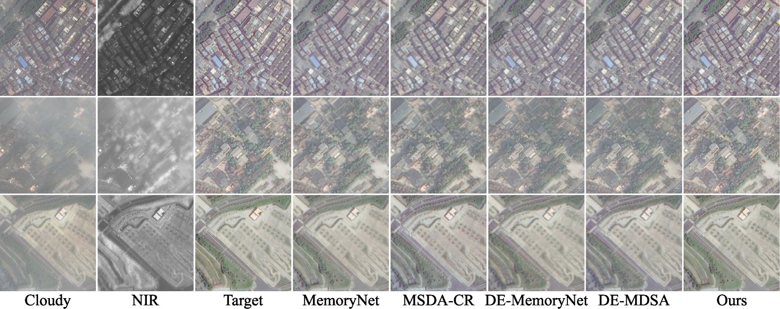
Figure 7: Additional visual results on the CUHK-CR1 dataset.

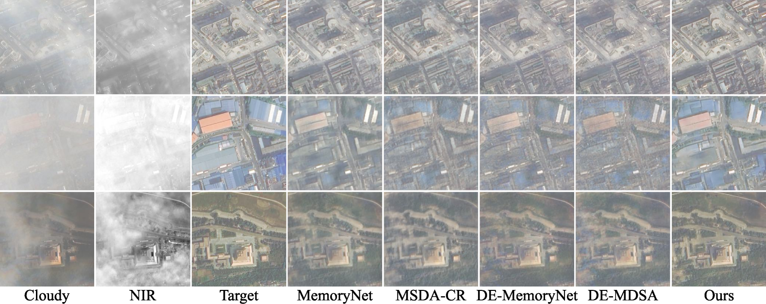
Figure 8: Additional visual results on the CUHK-CR2 dataset.

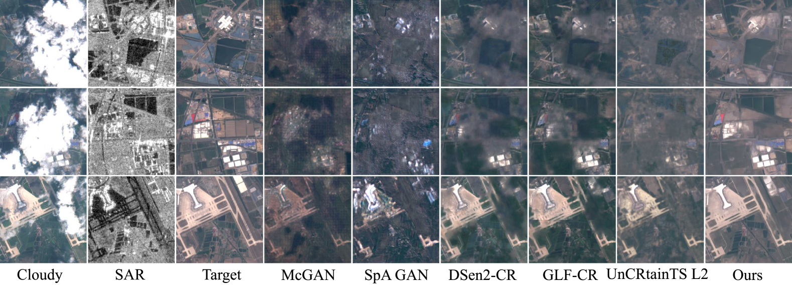
Figure 9: Additional visual results on the SEN12MS-CR dataset. As GLF-CR [xu2022glf] can only process $128\times 128$ images, unlike others ($256\times 256$), we divide each image into four parts, process them individually, and merge the results. Optical image brightness is linearly enhanced for visualization.

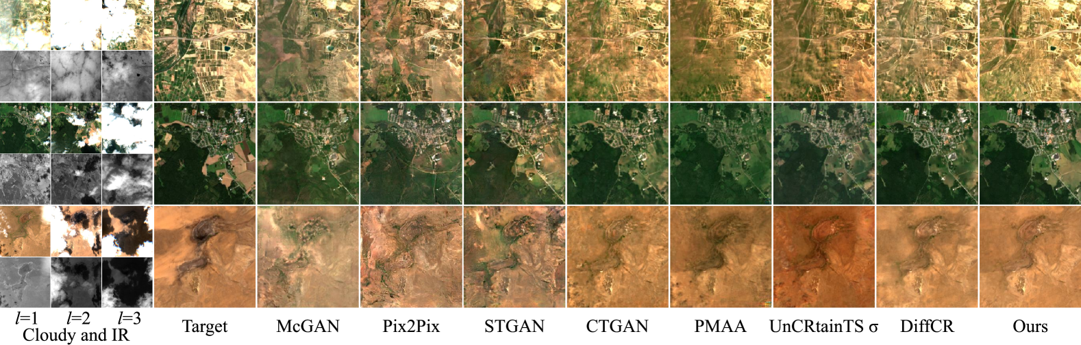
Figure 10: Additional visual results on the Sen2_MTC_New dataset.

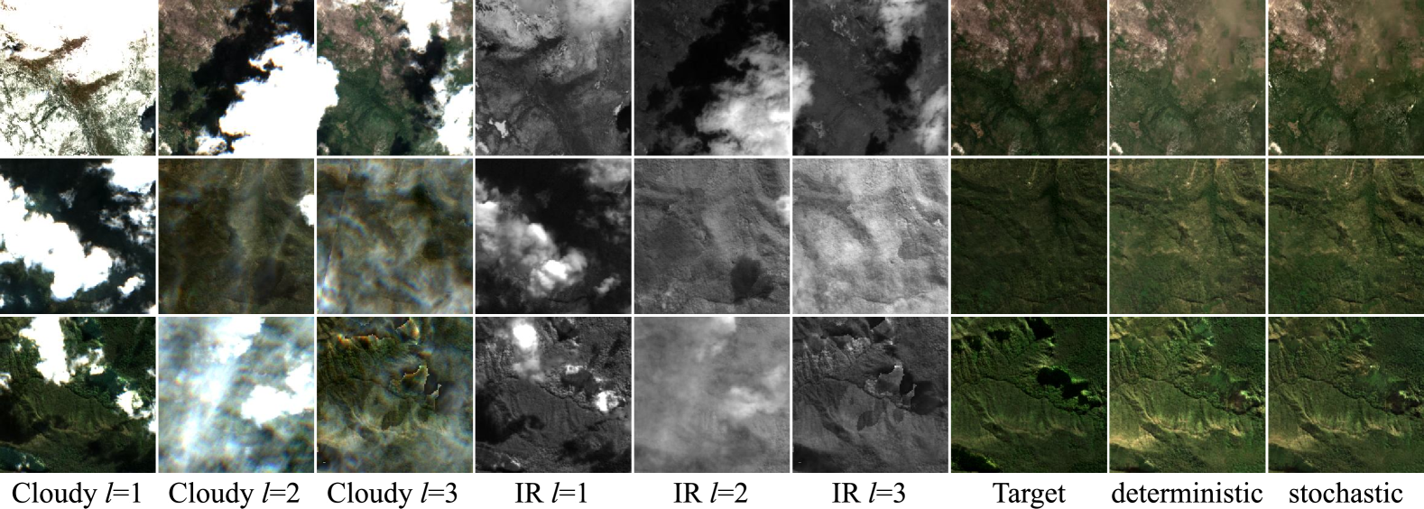
Figure 11: Visual results generated by the stochastic sampler and the deterministic sampler. For the deterministic sampler, we set $N=5$, $\sigma_{\text{min}}=0.001$ and $\sigma_{\text{max}}=100$. For the stochastic sampler, we set $N=5$, $\sigma_{\text{min}}=0.001$, $\sigma_{\text{max}}=100$, $S_{\text{churn}}=1.0$, $S_{\text{noise}}=1.0$, $S_{\text{tmin}}=0$ and $S_{\text{tmax}}=100$.

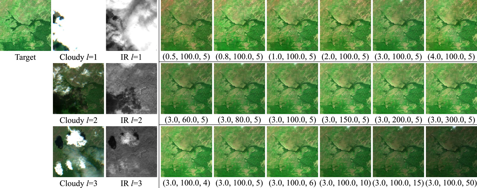
Figure 12: Visual results under different configurations of ($\alpha$, $\sigma_{\text{max}}$, $N$). For example, $(3.0,100.0,5)$ represents the restored results with $\alpha=3.0$, $\sigma_{\text{max}}=100.0$ and $N=5$.

Appendix C Experiments

C.1 Implementation Details

C.1.1 Datasets

The CUHK-CR1 and CUHK-CR2 datasets, introduced by [sui2024diffusion], consist of images captured by the Jilin-1 satellite with a size of $512\times 512$. CUHK-CR1 contains $668$ images of thin clouds, while CUHK-CR2 includes $559$ images of thick clouds. These two datasets collectively form the CUHK-CR dataset. With an ultra-high spatial resolution of $0.5$ m, the images encompass four bands: RGB and near-infrared (NIR). Following [sui2024diffusion], the CUHK-CR1 dataset is split into $534$ training and $134$ testing images, while CUHK-CR2 is divided into $448$ training and $111$ testing images. The images are in PNG format, with integer values in the range $[0,255]$.

The SEN12MS-CR dataset, introduced by [ebel2020multisensor], contains coregistered multi-spectral optical images with $13$ bands from Sentinel-2 satellite and SAR images with $2$ bands from Sentinel-1 satellite. Collected from 169 non-overlapping regions of interest (ROIs) across continents, each averaging approximately $52\times 40$ $\text{km}^{2}$ in size, the scenes of ROIs are divided into $256\times 256$ pixel patches, with $50\%$ spatial overlap. We use 114,050 images for training, 7,176 images for validation, and 7,899 images for testing. The dataset split follows previous works [ebel2020multisensor, ebel2023uncrtaints].

The Sen2_MTC_New dataset, introduced by [huang2022ctgan], consists of coregistered RGB and IR images across approximately 50 non-overlapping tiles. Each tile includes around 70 pairs of cropped $256\times 256$ pixel patches with pixel values ranging from 0 to $10,000$. Following [huang2022ctgan], the dataset is divided into $2,380$ images for training, $350$ for validation, and $687$ for testing.

C.1.2 Pre-Processing

As with common deep learning methods, images must be pre-processed before being input into our neural network. Given that datasets vary in their characteristics, we apply distinct pre-processing techniques to each one, following established practices. Below, we provide a detailed explanation.

The CUHK-CR1 and CUHK-CR2 datasets. Following [sui2024diffusion], we resize images from $512\times 512$ pixels to $256\times 256$ pixels. Subsequently, the pixel values are rescaled to a range of $[-1,1]$.

The Sen2_MTC_New dataset. Following [huang2022ctgan], the pixel values of images are initially scaled to the $[0,1]$ range by dividing by $10,000$, then normalized using a mean of $0.5$ and a standard deviation of $0.5$. For the training split, data augmentation includes random flips and a 90-degree rotation every four images.

The SEN12MS-CR dataset. Following [ebel2022sen12ms], the pixel values of SAR and optical images are clipped to the ranges of $[-25,0]$ and $[0,10000]$, respectively. However, we rescale the pixel values of all images to the range of $[-1,1]$ to achieve centrosymmetric pixel values, which is different from [ebel2022sen12ms].

C.1.3 Configuration

The optimal configuration is detailed in Tab. 5. The number of input channels is the sum of channels from noisy corrupted images, auxiliary modal images, and original corrupted images, as shown in Fig. 3. The table lists these channels as (input noisy corrupted image channels + input auxiliary modal image channels + input original corrupted image channels). For example, in the Input Channels row in Tab. 5, $28(=13+2+13)$ means that the noisy corrupted image has 13 channels, the auxiliary modal image has 2 channels and the original corrupted image has 13 channels. Notably, in CUHK-CR1 and CUHK-CR2 datasets, we reconstruct RGB and NIR channels following established methods, incorporating the NIR channel into the noisy corrupted image input rather than treated as auxiliary data. Consequently, the auxiliary modal image channel count for these datasets is zero.

C.1.4 Evaluation Metrics in Theory

To comprehensively evaluate the performance, we employ multiple metrics including peak signal-to-noise ratio (PSNR), structural similarity index measure (SSIM) [wang2004image], mean absolute error (MAE), spectral angle mapper (SAM) [kruse1993spectral], and learned perceptual image patch similarity (LPIPS) [zhang2018unreasonable]. The precise computational formulations of these metrics are as follows:

$$\text{PSNR}(\boldsymbol{y},\hat{\boldsymbol{y}}) =20\log_{10}\left(\cfrac{1}{\text{RMSE}(\boldsymbol{y},\hat{\boldsymbol{y}})}\right),$$ (89)

$$\text{SSIM}(\boldsymbol{y},\hat{\boldsymbol{y}}) =\cfrac{\left(2\mu_{\boldsymbol{y}}\mu_{\hat{\boldsymbol{y}}}+c_{1}\right)\left(2\sigma_{\boldsymbol{y}\hat{\boldsymbol{y}}}+c_{2}\right)}{\left(\mu_{\boldsymbol{y}}^{2}+\mu_{\hat{\boldsymbol{y}}}^{2}+c_{1}\right)\left(\sigma_{\boldsymbol{y}}^{2}+\sigma_{\hat{\boldsymbol{y}}}^{2}+c_{2}\right)},$$ (90)

$$\text{MAE}(\boldsymbol{y},\hat{\boldsymbol{y}}) ={\cfrac{1}{C\cdot H\cdot W}\sum_{c=1}^{C}{\sum_{h=1}^{H}{\sum_{w=1}^{W}{\lvert{\boldsymbol{y}_{c,h,w}-\hat{\boldsymbol{y}}_{c,h,w}}\rvert}}}},$$ (91)

$$\text{SAM}(\boldsymbol{y},\hat{\boldsymbol{y}}) =\cos^{-1}\left(\cfrac{\sum_{c=1}^{C}{\sum_{h=1}^{H}{\sum_{w=1}^{W}{{\boldsymbol{y}_{c,h,w}\cdot\hat{\boldsymbol{y}}_{c,h,w}}}}}}{\sqrt{\sum_{c=1}^{C}{\sum_{h=1}^{H}{\sum_{w=1}^{W}{\boldsymbol{y}_{c,h,w}^{2}}}}\cdot\sum_{c=1}^{C}{\sum_{h=1}^{H}{\sum_{w=1}^{W}{\hat{\boldsymbol{y}}_{c,h,w}^{2}}}}}}\right),$$ (92)

$$\text{LPIPS}(\boldsymbol{y},\hat{\boldsymbol{y}}) =\sum_{i}\cfrac{1}{H_{i}\cdot W_{i}}\sum_{h=1}^{H}{\sum_{w=1}^{W}{\left\|w_{i}\odot\left(\hat{\boldsymbol{y}}_{h,w}^{i}-\boldsymbol{y}_{h,w}^{i}\right)\right\|}_{2}^{2}}$$ (93)

where

$$\text{RMSE}(\boldsymbol{y},\hat{\boldsymbol{y}})=\sqrt{\cfrac{1}{C\cdot H\cdot W}\sum_{c=1}^{C}{\sum_{h=1}^{H}{\sum_{w=1}^{W}{{\left(\boldsymbol{y}_{c,h,w}-\hat{\boldsymbol{y}}_{c,h,w}\right)}^{2}}}}}.$$ (94)

Here, we denote the predicted image as $\hat{\boldsymbol{y}}$ and the ground truth image as $\boldsymbol{y}$. with channel number $C$, height $H$ and width $W$. The notation $\boldsymbol{y}_{c,h,w}$ and $\hat{\boldsymbol{y}}_{c,h,w}$ refers to a specific pixel in $\boldsymbol{y}$ and $\hat{\boldsymbol{y}}$, indicated by subscript $c$, $h$, $w$. In Eq. 90, $\mu_{\boldsymbol{y}}$ and $\mu_{\hat{\boldsymbol{y}}}$ represent the means, and $\sigma_{\boldsymbol{y}}$ and $\sigma_{\hat{\boldsymbol{y}}}$ are the standard deviations of $\boldsymbol{y}$ and $\hat{\boldsymbol{y}}$, respectively. The covariance is symbolized by $\sigma_{\boldsymbol{y}\hat{\boldsymbol{y}}}$. The constants $c_{1}$ and $c_{2}$ stabilize the calculations. To compute LPIPS [zhang2018unreasonable], a pre-trained network $\mathcal{F}$ processes $\boldsymbol{y}$ and $\hat{\boldsymbol{y}}$ to derive intermediate embeddings across multiple layers. The activations are normalized, scaled by a vector $w$, and the L2 distance between embeddings of $\boldsymbol{y}$ and $\hat{\boldsymbol{y}}$ is calculated and averaged over spatial dimensions and layers as the final LPIPS value, as shown in Eq. 93. In Eq. 93, $i$ indicates the layer of $\mathcal{F}$, with $H_{i}$, $W_{i}$, and $w_{i}$ being the height, width, and scaling factor at the layer $i$. The embeddings at the position $(h,w)$ and the layer $i$ are denoted as $\hat{\boldsymbol{y}}_{h,w}^{i}$ and $\boldsymbol{y}_{h,w}^{i}$. We use the official implementations of [zhang2018unreasonable] to calculate the value of LPIPS.

C.1.5 Evaluation Metrics in Practice

Although the theoretical methods for these evaluation metrics are consistent across datasets, practical calculations may vary due to pre-processing, post-processing, etc. To ensure a fair comparison, we apply different computing methods for each dataset, in line with prior research. Detailed explanations for each dataset are provided here.

The CUHK-CR1 and CUHK-CR2 datasets. Following [sui2024diffusion], we scale the pixel values of the restored and ground truth images, i.e. $\hat{\boldsymbol{y}}$ and $\boldsymbol{y}$, to the range $[0,255]$, and clamp any out-of-range values. These pixel values are then converted to unsigned integers. PSNR is calculated using all channels, while SSIM and LPIPS are first calculated for each channel and then averaged. To calculate LPIPS, we employ a pre-trained AlexNet [krizhevsky2012imagenet] as $\mathcal{F}$.

The Sen2_MTC_New dataset. We adopt the DiffCR [zou2024diffcr] approach by rescaling the pixel values of the restored and ground truth images to the range $[0,1000]$, clipping values outside $[0,2000]$, and then rescaling back to $[0,1]$. These processed images are used to compute PSNR and SSIM across all channels. For LPIPS, the input images are further rescaled to $[-1,1]$ and processed using a pre-trained AlexNet [krizhevsky2012imagenet] as $\mathcal{F}$.

The SEN12MS-CR dataset. All the images are rescaled to $[0,1]$. Then, the rescaled images are used to compute PSNR, SSIM, MAE, and SAM, with all channels used.

C.1.6 Reproducing Details

For closed-source methods, we use the metric values they report. In contrast, for certain open-source methods, we implement the algorithms ourselves and present visual results in Fig. 4. When implementing previous methods, if pre-trained weights are available, we directly use them; otherwise, we retrain the models from scratch. Below, we briefly outline the implementation details of the reproduced methods.

The CUHK-CR1 and CUHK-CR2 datasets. The CUHK-CR1 and CUHK-CR2 datasets are relatively new, with limited prior research [sui2024diffusion]. The authors evaluate five existing methods: SpA-GAN [pan2020cloud], AMGAN-CR [xu2022attention], CVAE [ding2022uncertainty], MemoryNet [zhang2023memory], and MSDA-CR [yu2022cloud], alongside their proposed methods, DE-MemoryNet and DE-MSDA [sui2024diffusion], on these two dataset. In [sui2024diffusion], metrics for all methods are reported, with pre-trained weights provided only for MemoryNet and MSDA-CR. Consequently, we use these weights and retrain DE-MemoryNet and DE-MSDA to present visual results in Fig. 4. DE-MSDA is excluded from Fig. 4 as it performs worse than DE-MemoryNet, despite being introduced in the same study.

The SEN12MS-CR dataset. As McGAN [enomoto2017filmy] and SpA GAN [pan2020cloud] do not have pre-trained weights for this dataset, we retrain them and present the visual results in Fig. 4. In contrast, pre-trained weights for DSen2-CR [meraner2020cloud], GLF-CR [xu2022glf], and UnCRtainTS [ebel2023uncrtaints] are available and have also been used for visualization in Fig. 4. Notably, GLF-CR [xu2022glf] operates on $128\times 128$ images, while other methods use $256\times 256$ images. To ensure consistency, we divide each image into four segments, process them independently, and subsequently merge them for visualization, as shown in Fig. 4. The performance metrics for all previous methods on this dataset are cited from [ebel2023uncrtaints] and [zou2024diffcr].

The Sen2_MTC_New dataset. Metrics values are cited from [huang2022ctgan], [zou2023pmaa], and [zou2024diffcr]. We retrain McGAN [enomoto2017filmy], Pix2Pix [isola2017image-to-image], STGAN [sarukkai2020cloud] and UnCRtainTS [ebel2023uncrtaints], while using pre-trained weights of CTGAN [huang2022ctgan], PMAA [zou2023pmaa], and DiffCR [zou2024diffcr] for visualization in Fig. 4.

C.2 Efficiency Analysis

Table 6: The Comparison of Params (the number of parameters) and MACs (multiply-accumulate operations).

(a) SEN12MS-CR	GLF-CR	UnCRtainTS L2	DiffCR	EMRDM
Params (M)	14.827	0.519	22.96	39.13
MACs (G)	245.28	28.02	29.37	83.57

(b) CUHK-CR	MemoryNet	MSDA-CR	DE	EMRDM
Params (M)	3.64	3.91	36.80	39.13
MACs (G)	548.65	53.45	199.15	83.33

(c) Sen2_MTC_New	STGAN	CTGAN	CR-TS Net	PMAA	UnCRtainTS	DDPM-CR	DiffCR	EMRDM
Params (M)	231.93	642.92	38.68	3.45	0.56	445.44	22.91	148.88
MACs (G)	1094.94	632.05	7602.97	92.35	37.16	852.37	45.86	74.39

We first present a comparative analysis of parameter counts (Params) and multiply-accumulate operations (MACs) of our proposed method against recent state-of-the-art approaches. in Tab. 6 across the four datasets. Our analysis excludes early methods due to their significantly inferior performance compared to EMRDM and the unavailability or irreproducibility of their detailed implementations. All MACs are computed with a batch size of 1 and an input image resolution of $256\times 256$ to ensure fair comparisons. It should be noted that although GLF-CR [xu2022glf] typically operates on $128\times 128$ resolution images, we evaluated it at $256\times 256$ resolution for efficiency analysis to maintain consistency across comparisons. Moreover, for DiffCR, which lacks official implementation details for the SEN12MS-CR dataset, we reproduce it on this dataset based on the description outlined in [zou2024diffcr] and report the corresponding Params and MACs in Tab. 6. The entries labeled ”DE” in Tab. 6 denote DE-MemoryNet and DE-MSDA [sui2024diffusion], which share identical Params and MACs. The results of efficiency analysis demonstrate that EMRDM achieves performance gains with reasonable increments in Params and MACs, particularly for mono-temporal tasks. While multi-temporal tasks necessitate additional parameters of EMRDM to effectively model complex temporal dependencies in image sequences, the corresponding MACs remain within reasonable bounds for real-world applications.

We further analyzed the training and sampling time of EMRDM across the four datasets. For standardization, we use the configurations in Tab. 5 and measured training time per batch with batch size unchanged and sampling time per image with batch size changed to 1. All experiments are conducted on a single NVIDIA RTX 4090 GPU to ensure fair comparisons. Per-batch training times measure 1,410.5 ms (CUHK-CR1), 1,237.7 ms (CUHK-CR2), 1,230.5 ms (SEN12MS-CR), and 204.7 ms (Sen2_MTC_New), with per-image sampling times of 131.2 ms (CUHK-CR1), 128.0 ms (CUHK-CR2), 136.4 ms (SEN12MS-CR), and 173.1 ms (Sen2_MTC_New). These timing measurements are hardware-dependent and may fluctuate. Hence, we report only mean values. Notable, sampling time is particularly significant since training occurs only once, while sampling is performed repeatedly in practical CR applications. The measured sampling times demonstrate that EMRDM meets real-time requirements for CR applications, a critical factor for remote sensing, while delivering significant performance advantages.

C.3 Additional Results

This section presents additional results, including visual examples from the CUHK-CR1, CUHK-CR2, SEN12MS-CR, and Sen2_MTC_New datasets in Fig. 7, Fig. 8, Fig. 9, and Fig. 10, respectively. Visual comparisons using our stochastic and deterministic samplers are shown in Fig. 11. Additionally, results under varying settings of $(\alpha,\sigma_{\text{max}},N)$ are provided in Fig. 12.

References

- Bansal et al. [2024] Arpit Bansal, Eitan Borgnia, Hong-Min Chu, Jie Li, Hamid Kazemi, Furong Huang, Micah Goldblum, Jonas Geiping, and Tom Goldstein. Cold diffusion: Inverting arbitrary image transforms without noise. Advances in Neural Information Processing Systems, 36, 2024.
- Bao et al. [2023] Fan Bao, Shen Nie, Kaiwen Xue, Yue Cao, Chongxuan Li, Hang Su, and Jun Zhu. All are worth words: A vit backbone for diffusion models. In Proceedings of the IEEE/CVF conference on computer vision and pattern recognition, pages 22669–22679, 2023.
- Bau et al. [2019] David Bau, Jun-Yan Zhu, Jonas Wulff, William Peebles, Hendrik Strobelt, Bolei Zhou, and Antonio Torralba. Seeing what a gan cannot generate. In Proceedings of the IEEE/CVF International Conference on Computer Vision (ICCV), 2019.
- Bermudez et al. [2018] Jose D Bermudez, Patrick Nigri Happ, Dario Augusto Borges Oliveira, and Raul Queiroz Feitosa. Sar to optical image synthesis for cloud removal with generative adversarial networks. ISPRS Annals of the Photogrammetry, Remote Sensing and Spatial Information Sciences, 4:5–11, 2018.
- Bishop [1995] Christopher M Bishop. Neural networks for pattern recognition. Oxford university press, 1995.
- Blau and Michaeli [2018] Yochai Blau and Tomer Michaeli. The perception-distortion tradeoff. In Proceedings of the IEEE conference on computer vision and pattern recognition, pages 6228–6237, 2018.
- Chen et al. [2020] Yang Chen, Qihao Weng, Luliang Tang, Xia Zhang, Muhammad Bilal, and Qingquan Li. Thick clouds removing from multitemporal landsat images using spatiotemporal neural networks. IEEE Transactions on Geoscience and Remote Sensing, 60:1–14, 2020.
- Choi et al. [2021] Jooyoung Choi, Sungwon Kim, Yonghyun Jeong, Youngjune Gwon, and Sungroh Yoon. Ilvr: Conditioning method for denoising diffusion probabilistic models. In Proceedings of the IEEE/CVF International Conference on Computer Vision, pages 14367–14376, 2021.
- Crowson et al. [2024] Katherine Crowson, Stefan Andreas Baumann, Alex Birch, Tanishq Mathew Abraham, Daniel Z Kaplan, and Enrico Shippole. Scalable high-resolution pixel-space image synthesis with hourglass diffusion transformers. In Forty-first International Conference on Machine Learning, 2024.
- Delbracio and Milanfar [2023] Mauricio Delbracio and Peyman Milanfar. Inversion by direct iteration: An alternative to denoising diffusion for image restoration. Transactions on Machine Learning Research, 2023. Featured Certification.
- Dhariwal and Nichol [2021] Prafulla Dhariwal and Alexander Nichol. Diffusion models beat gans on image synthesis. Advances in neural information processing systems, 34:8780–8794, 2021.
- Ding et al. [2022] Haidong Ding, Yue Zi, and Fengying Xie. Uncertainty-based thin cloud removal network via conditional variational autoencoders. In Proceedings of the Asian Conference on Computer Vision, pages 469–485, 2022.
- Ebel et al. [2020] Patrick Ebel, Andrea Meraner, Michael Schmitt, and Xiao Xiang Zhu. Multisensor data fusion for cloud removal in global and all-season sentinel-2 imagery. IEEE Transactions on Geoscience and Remote Sensing, 59(7):5866–5878, 2020.
- Ebel et al. [2022] Patrick Ebel, Yajin Xu, Michael Schmitt, and Xiao Xiang Zhu. Sen12ms-cr-ts: A remote-sensing data set for multimodal multitemporal cloud removal. IEEE Transactions on Geoscience and Remote Sensing, 60:1–14, 2022.
- Ebel et al. [2023] Patrick Ebel, Vivien Sainte Fare Garnot, Michael Schmitt, Jan Dirk Wegner, and Xiao Xiang Zhu. Uncrtaints: Uncertainty quantification for cloud removal in optical satellite time series. In Proceedings of the IEEE/CVF Conference on Computer Vision and Pattern Recognition, pages 2086–2096, 2023.
- Enomoto et al. [2017] Kenji Enomoto, Ken Sakurada, Weimin Wang, Hiroshi Fukui, Masashi Matsuoka, Ryosuke Nakamura, and Nobuo Kawaguchi. Filmy cloud removal on satellite imagery with multispectral conditional generative adversarial nets. In Proceedings of the IEEE conference on computer vision and pattern recognition workshops, pages 48–56, 2017.
- Gao et al. [2020] Jianhao Gao, Qiangqiang Yuan, Jie Li, Hai Zhang, and Xin Su. Cloud removal with fusion of high resolution optical and sar images using generative adversarial networks. Remote Sensing, 12(1):191, 2020.
- Garnot and Landrieu [2020] Vivien Sainte Fare Garnot and Loic Landrieu. Lightweight temporal self-attention for classifying satellite images time series. In Advanced Analytics and Learning on Temporal Data: 5th ECML PKDD Workshop, AALTD 2020, Ghent, Belgium, September 18, 2020, Revised Selected Papers 6, pages 171–181. Springer, 2020.
- Garnot and Landrieu [2021] Vivien Sainte Fare Garnot and Loic Landrieu. Panoptic segmentation of satellite image time series with convolutional temporal attention networks. In Proceedings of the IEEE/CVF International Conference on Computer Vision, pages 4872–4881, 2021.
- Goodfellow et al. [2014] Ian Goodfellow, Jean Pouget-Abadie, Mehdi Mirza, Bing Xu, David Warde-Farley, Sherjil Ozair, Aaron Courville, and Yoshua Bengio. Generative adversarial nets. Advances in neural information processing systems, 27, 2014.
- Grohnfeldt et al. [2018] Claas Grohnfeldt, Michael Schmitt, and Xiaoxiang Zhu. A conditional generative adversarial network to fuse sar and multispectral optical data for cloud removal from sentinel-2 images. In IGARSS 2018-2018 IEEE International Geoscience and Remote Sensing Symposium, pages 1726–1729. IEEE, 2018.
- Ho and Salimans [2021] Jonathan Ho and Tim Salimans. Classifier-free diffusion guidance. In NeurIPS 2021 Workshop on Deep Generative Models and Downstream Applications, 2021.
- Ho et al. [2020] Jonathan Ho, Ajay Jain, and Pieter Abbeel. Denoising diffusion probabilistic models. Advances in neural information processing systems, 33:6840–6851, 2020.
- Huang and Wu [2022] Gi-Luen Huang and Pei-Yuan Wu. Ctgan: Cloud transformer generative adversarial network. In 2022 IEEE International Conference on Image Processing (ICIP), pages 511–515. IEEE, 2022.
- Huang et al. [2023] Lei Huang, Jie Qin, Yi Zhou, Fan Zhu, Li Liu, and Ling Shao. Normalization techniques in training dnns: Methodology, analysis and application. IEEE transactions on pattern analysis and machine intelligence, 45(8):10173–10196, 2023.
- Huang et al. [2024] Wenli Huang, Ye Deng, Yang Wu, and Jinjun Wang. Attentive contextual attention for cloud removal. IEEE Transactions on Geoscience and Remote Sensing, 2024.
- Hyvärinen and Dayan [2005] Aapo Hyvärinen and Peter Dayan. Estimation of non-normalized statistical models by score matching. Journal of Machine Learning Research, 6(4), 2005.
- Isola et al. [2017] Phillip Isola, Jun-Yan Zhu, Tinghui Zhou, and Alexei A. Efros. Image-to-image translation with conditional adversarial networks. In Proceedings of the IEEE Conference on Computer Vision and Pattern Recognition (CVPR), 2017.
- Jing et al. [2023] Ran Jing, Fuzhou Duan, Fengxian Lu, Miao Zhang, and Wenji Zhao. Denoising diffusion probabilistic feature-based network for cloud removal in sentinel-2 imagery. Remote Sensing, 15(9):2217, 2023.
- Karras et al. [2020] Tero Karras, Miika Aittala, Janne Hellsten, Samuli Laine, Jaakko Lehtinen, and Timo Aila. Training generative adversarial networks with limited data. Advances in Neural Information Processing Systems, 33:12104–12114, 2020.
- Karras et al. [2022] Tero Karras, Miika Aittala, Timo Aila, and Samuli Laine. Elucidating the design space of diffusion-based generative models. Advances in neural information processing systems, 35:26565–26577, 2022.
- Kawar et al. [2022] Bahjat Kawar, Michael Elad, Stefano Ermon, and Jiaming Song. Denoising diffusion restoration models. Advances in Neural Information Processing Systems, 35:23593–23606, 2022.
- King et al. [2013] Michael D King, Steven Platnick, W Paul Menzel, Steven A Ackerman, and Paul A Hubanks. Spatial and temporal distribution of clouds observed by modis onboard the terra and aqua satellites. IEEE transactions on geoscience and remote sensing, 51(7):3826–3852, 2013.
- Kussul et al. [2017] Nataliia Kussul, Mykola Lavreniuk, Sergii Skakun, and Andrii Shelestov. Deep learning classification of land cover and crop types using remote sensing data. IEEE Geoscience and Remote Sensing Letters, 14(5):778–782, 2017.
- Li et al. [2023a] Congyu Li, Xinxin Liu, and Shutao Li. Transformer meets gan: Cloud-free multispectral image reconstruction via multi-sensor data fusion in satellite images. IEEE Transactions on Geoscience and Remote Sensing, 2023a.
- Li et al. [2023b] Xin Li, Yulin Ren, Xin Jin, Cuiling Lan, Xingrui Wang, Wenjun Zeng, Xinchao Wang, and Zhibo Chen. Diffusion models for image restoration and enhancement–a comprehensive survey. arXiv preprint arXiv:2308.09388, 2023b.
- Lin et al. [2012] Chao-Hung Lin, Po-Hung Tsai, Kang-Hua Lai, and Jyun-Yuan Chen. Cloud removal from multitemporal satellite images using information cloning. IEEE transactions on geoscience and remote sensing, 51(1):232–241, 2012.
- Liu et al. [2023] Guan-Horng Liu, Arash Vahdat, De-An Huang, Evangelos A Theodorou, Weili Nie, and Anima Anandkumar. I2sb: image-to-image schrödinger bridge. In Proceedings of the 40th International Conference on Machine Learning, pages 22042–22062, 2023.
- Liu et al. [2024] Jiawei Liu, Qiang Wang, Huijie Fan, Yinong Wang, Yandong Tang, and Liangqiong Qu. Residual denoising diffusion models. In Proceedings of the IEEE/CVF Conference on Computer Vision and Pattern Recognition, pages 2773–2783, 2024.
- Lugmayr et al. [2022] Andreas Lugmayr, Martin Danelljan, Andres Romero, Fisher Yu, Radu Timofte, and Luc Van Gool. Repaint: Inpainting using denoising diffusion probabilistic models. In Proceedings of the IEEE/CVF conference on computer vision and pattern recognition, pages 11461–11471, 2022.
- Luo et al. [2023a] Ziwei Luo, Fredrik K. Gustafsson, Zheng Zhao, Jens Sjölund, and Thomas B. Schön. Image restoration with mean-reverting stochastic differential equations. In Proceedings of the 40th International Conference on Machine Learning, pages 23045–23066. PMLR, 2023a.
- Luo et al. [2023b] Ziwei Luo, Fredrik K Gustafsson, Zheng Zhao, Jens Sjölund, and Thomas B Schön. Refusion: Enabling large-size realistic image restoration with latent-space diffusion models. In Proceedings of the IEEE/CVF conference on computer vision and pattern recognition, pages 1680–1691, 2023b.
- Meraner et al. [2020] Andrea Meraner, Patrick Ebel, Xiao Xiang Zhu, and Michael Schmitt. Cloud removal in sentinel-2 imagery using a deep residual neural network and sar-optical data fusion. ISPRS Journal of Photogrammetry and Remote Sensing, 166:333–346, 2020.
- Mirza [2014] Mehdi Mirza. Conditional generative adversarial nets. arXiv preprint arXiv:1411.1784, 2014.
- Pan [2020] Heng Pan. Cloud removal for remote sensing imagery via spatial attention generative adversarial network. arXiv preprint arXiv:2009.13015, 2020.
- Peebles and Xie [2023] William Peebles and Saining Xie. Scalable diffusion models with transformers. In Proceedings of the IEEE/CVF International Conference on Computer Vision, pages 4195–4205, 2023.
- Rombach et al. [2022] Robin Rombach, Andreas Blattmann, Dominik Lorenz, Patrick Esser, and Björn Ommer. High-resolution image synthesis with latent diffusion models. In Proceedings of the IEEE/CVF conference on computer vision and pattern recognition, pages 10684–10695, 2022.
- Rußwurm and Korner [2017] Marc Rußwurm and Marco Korner. Temporal vegetation modelling using long short-term memory networks for crop identification from medium-resolution multi-spectral satellite images. In Proceedings of the IEEE conference on computer vision and pattern recognition workshops, pages 11–19, 2017.
- Saharia et al. [2022a] Chitwan Saharia, William Chan, Huiwen Chang, Chris Lee, Jonathan Ho, Tim Salimans, David Fleet, and Mohammad Norouzi. Palette: Image-to-image diffusion models. In ACM SIGGRAPH 2022 conference proceedings, pages 1–10, 2022a.
- Saharia et al. [2022b] Chitwan Saharia, Jonathan Ho, William Chan, Tim Salimans, David J Fleet, and Mohammad Norouzi. Image super-resolution via iterative refinement. IEEE transactions on pattern analysis and machine intelligence, 45(4):4713–4726, 2022b.
- Salimans et al. [2016] Tim Salimans, Ian Goodfellow, Wojciech Zaremba, Vicki Cheung, Alec Radford, and Xi Chen. Improved techniques for training gans. Advances in neural information processing systems, 29, 2016.
- Sarukkai et al. [2020] Vishnu Sarukkai, Anirudh Jain, Burak Uzkent, and Stefano Ermon. Cloud removal from satellite images using spatiotemporal generator networks. In Proceedings of the IEEE/CVF Winter Conference on Applications of Computer Vision, pages 1796–1805, 2020.
- Sintarasirikulchai et al. [2018] Wassana Sintarasirikulchai, Teerasit Kasetkasem, Tsuyoshi Isshiki, Thitiporn Chanwimaluang, and Preesan Rakwatin. A multi-temporal convolutional autoencoder neural network for cloud removal in remote sensing images. In 2018 15th International Conference on Electrical Engineering/Electronics, Computer, Telecommunications and Information Technology (ECTI-CON), pages 360–363. IEEE, 2018.
- Song et al. [2023a] Jiaming Song, Arash Vahdat, Morteza Mardani, and Jan Kautz. Pseudoinverse-guided diffusion models for inverse problems. In International Conference on Learning Representations, 2023a.
- Song and Ermon [2019] Yang Song and Stefano Ermon. Generative modeling by estimating gradients of the data distribution. Advances in neural information processing systems, 32, 2019.
- Song et al. [2021] Yang Song, Jascha Sohl-Dickstein, Diederik P Kingma, Abhishek Kumar, Stefano Ermon, and Ben Poole. Score-based generative modeling through stochastic differential equations. In International Conference on Learning Representations, 2021.
- Song et al. [2023b] Yang Song, Prafulla Dhariwal, Mark Chen, and Ilya Sutskever. Consistency models. In International Conference on Machine Learning, pages 32211–32252. PMLR, 2023b.
- Sui et al. [2024] Jialu Sui, Yiyang Ma, Wenhan Yang, Xiaokang Zhang, Man-On Pun, and Jiaying Liu. Diffusion enhancement for cloud removal in ultra-resolution remote sensing imagery. IEEE Transactions on Geoscience and Remote Sensing, 2024.
- Vakalopoulou et al. [2015] Maria Vakalopoulou, Konstantinos Karantzalos, Nikos Komodakis, and Nikos Paragios. Building detection in very high resolution multispectral data with deep learning features. In 2015 IEEE international geoscience and remote sensing symposium (IGARSS), pages 1873–1876. IEEE, 2015.
- Wang et al. [2023] Yinhuai Wang, Jiwen Yu, and Jian Zhang. Zero-shot image restoration using denoising diffusion null-space model. In The Eleventh International Conference on Learning Representations, 2023.
- Xia et al. [2023] Bin Xia, Yulun Zhang, Shiyin Wang, Yitong Wang, Xinglong Wu, Yapeng Tian, Wenming Yang, and Luc Van Gool. Diffir: Efficient diffusion model for image restoration. In Proceedings of the IEEE/CVF International Conference on Computer Vision, pages 13095–13105, 2023.
- Xiong et al. [2023] Quan Xiong, Guoqing Li, Xiaochuang Yao, and Xiaodong Zhang. Sar-to-optical image translation and cloud removal based on conditional generative adversarial networks: Literature survey, taxonomy, evaluation indicators, limits and future directions. Remote Sensing, 15(4):1137, 2023.
- Xu et al. [2022a] Fang Xu, Yilei Shi, Patrick Ebel, Lei Yu, Gui-Song Xia, Wen Yang, and Xiao Xiang Zhu. Glf-cr: Sar-enhanced cloud removal with global–local fusion. ISPRS Journal of Photogrammetry and Remote Sensing, 192:268–278, 2022a.
- Xu et al. [2015] Meng Xu, Mark Pickering, Antonio J Plaza, and Xiuping Jia. Thin cloud removal based on signal transmission principles and spectral mixture analysis. IEEE Transactions on Geoscience and Remote Sensing, 54(3):1659–1669, 2015.
- Xu et al. [2019] Meng Xu, Xiuping Jia, Mark Pickering, and Sen Jia. Thin cloud removal from optical remote sensing images using the noise-adjusted principal components transform. ISPRS Journal of Photogrammetry and Remote Sensing, 149:215–225, 2019.
- Xu et al. [2022b] Meng Xu, Furong Deng, Sen Jia, Xiuping Jia, and Antonio J Plaza. Attention mechanism-based generative adversarial networks for cloud removal in landsat images. Remote sensing of environment, 271:112902, 2022b.
- Yu et al. [2022] Weikang Yu, Xiaokang Zhang, and Man-On Pun. Cloud removal in optical remote sensing imagery using multiscale distortion-aware networks. IEEE Geoscience and Remote Sensing Letters, 19:1–5, 2022.
- Yuan et al. [2020] Qiangqiang Yuan, Huanfeng Shen, Tongwen Li, Zhiwei Li, Shuwen Li, Yun Jiang, Hongzhang Xu, Weiwei Tan, Qianqian Yang, Jiwen Wang, et al. Deep learning in environmental remote sensing: Achievements and challenges. Remote sensing of Environment, 241:111716, 2020.
- Yue et al. [2023] Zongsheng Yue, Jianyi Wang, and Chen Change Loy. Resshift: Efficient diffusion model for image super-resolution by residual shifting. Advances in Neural Information Processing Systems, 36:13294–13307, 2023.
- Zhang et al. [2023] Xiao Feng Zhang, Chao Chen Gu, and Shan Ying Zhu. Memory augment is all you need for image restoration. arXiv preprint arXiv:2309.01377, 2023.
- Zhao and Jia [2023] Xiaohu Zhao and Kebin Jia. Cloud removal in remote sensing using sequential-based diffusion models. Remote Sensing, 15(11):2861, 2023.
- Zhu et al. [2017] Xiao Xiang Zhu, Devis Tuia, Lichao Mou, Gui-Song Xia, Liangpei Zhang, Feng Xu, and Friedrich Fraundorfer. Deep learning in remote sensing: A comprehensive review and list of resources. IEEE Geoscience and Remote Sensing Magazine, 5(4):8–36, 2017.
- Zou et al. [2023] Xuechao Zou, Kai Li, Junliang Xing, Pin Tao, and Yachao Cui. Pmaa: A progressive multi-scale attention autoencoder model for high-performance cloud removal from multi-temporal satellite imagery. In ECAI, pages 3165–3172, 2023.
- Zou et al. [2024] Xuechao Zou, Kai Li, Junliang Xing, Yu Zhang, Shiying Wang, Lei Jin, and Pin Tao. Diffcr: A fast conditional diffusion framework for cloud removal from optical satellite images. IEEE Transactions on Geoscience and Remote Sensing, 62:1–14, 2024.

References

- Bermudez et al. [2018] Jose D Bermudez, Patrick Nigri Happ, Dario Augusto Borges Oliveira, and Raul Queiroz Feitosa. Sar to optical image synthesis for cloud removal with generative adversarial networks. ISPRS Annals of the Photogrammetry, Remote Sensing and Spatial Information Sciences, 4:5–11, 2018.
- Crowson et al. [2024] Katherine Crowson, Stefan Andreas Baumann, Alex Birch, Tanishq Mathew Abraham, Daniel Z Kaplan, and Enrico Shippole. Scalable high-resolution pixel-space image synthesis with hourglass diffusion transformers. In Forty-first International Conference on Machine Learning, 2024.
- Delbracio and Milanfar [2023] Mauricio Delbracio and Peyman Milanfar. Inversion by direct iteration: An alternative to denoising diffusion for image restoration. Transactions on Machine Learning Research, 2023. Featured Certification.
- Dhariwal and Nichol [2021] Prafulla Dhariwal and Alexander Nichol. Diffusion models beat gans on image synthesis. Advances in neural information processing systems, 34:8780–8794, 2021.
- Ding et al. [2022] Haidong Ding, Yue Zi, and Fengying Xie. Uncertainty-based thin cloud removal network via conditional variational autoencoders. In Proceedings of the Asian Conference on Computer Vision, pages 469–485, 2022.
- Ebel et al. [2020] Patrick Ebel, Andrea Meraner, Michael Schmitt, and Xiao Xiang Zhu. Multisensor data fusion for cloud removal in global and all-season sentinel-2 imagery. IEEE Transactions on Geoscience and Remote Sensing, 59(7):5866–5878, 2020.
- Ebel et al. [2022] Patrick Ebel, Yajin Xu, Michael Schmitt, and Xiao Xiang Zhu. Sen12ms-cr-ts: A remote-sensing data set for multimodal multitemporal cloud removal. IEEE Transactions on Geoscience and Remote Sensing, 60:1–14, 2022.
- Ebel et al. [2023] Patrick Ebel, Vivien Sainte Fare Garnot, Michael Schmitt, Jan Dirk Wegner, and Xiao Xiang Zhu. Uncrtaints: Uncertainty quantification for cloud removal in optical satellite time series. In Proceedings of the IEEE/CVF Conference on Computer Vision and Pattern Recognition, pages 2086–2096, 2023.
- Enomoto et al. [2017] Kenji Enomoto, Ken Sakurada, Weimin Wang, Hiroshi Fukui, Masashi Matsuoka, Ryosuke Nakamura, and Nobuo Kawaguchi. Filmy cloud removal on satellite imagery with multispectral conditional generative adversarial nets. In Proceedings of the IEEE conference on computer vision and pattern recognition workshops, pages 48–56, 2017.
- Gao et al. [2020] Jianhao Gao, Qiangqiang Yuan, Jie Li, Hai Zhang, and Xin Su. Cloud removal with fusion of high resolution optical and sar images using generative adversarial networks. Remote Sensing, 12(1):191, 2020.
- Gao et al. [2023] Sicheng Gao, Xuhui Liu, Bohan Zeng, Sheng Xu, Yanjing Li, Xiaoyan Luo, Jianzhuang Liu, Xiantong Zhen, and Baochang Zhang. Implicit diffusion models for continuous super-resolution. In Proceedings of the IEEE/CVF conference on computer vision and pattern recognition, pages 10021–10030, 2023.
- Grohnfeldt et al. [2018] Claas Grohnfeldt, Michael Schmitt, and Xiaoxiang Zhu. A conditional generative adversarial network to fuse sar and multispectral optical data for cloud removal from sentinel-2 images. In IGARSS 2018-2018 IEEE International Geoscience and Remote Sensing Symposium, pages 1726–1729. IEEE, 2018.
- Hang et al. [2023] Tiankai Hang, Shuyang Gu, Chen Li, Jianmin Bao, Dong Chen, Han Hu, Xin Geng, and Baining Guo. Efficient diffusion training via min-snr weighting strategy. In Proceedings of the IEEE/CVF International Conference on Computer Vision, pages 7441–7451, 2023.
- Ho et al. [2020] Jonathan Ho, Ajay Jain, and Pieter Abbeel. Denoising diffusion probabilistic models. Advances in neural information processing systems, 33:6840–6851, 2020.
- Hu et al. [2015] Gensheng Hu, Xiaoyi Li, and Dong Liang. Thin cloud removal from remote sensing images using multidirectional dual tree complex wavelet transform and transfer least square support vector regression. Journal of Applied Remote Sensing, 9(1):095053–095053, 2015.
- Huang and Wu [2022] Gi-Luen Huang and Pei-Yuan Wu. Ctgan: Cloud transformer generative adversarial network. In 2022 IEEE International Conference on Image Processing (ICIP), pages 511–515. IEEE, 2022.
- Hyvärinen and Dayan [2005] Aapo Hyvärinen and Peter Dayan. Estimation of non-normalized statistical models by score matching. Journal of Machine Learning Research, 6(4), 2005.
- Hyvärinen et al. [2009] Aapo Hyvärinen, Jarmo Hurri, Patrik O Hoyer, Aapo Hyvärinen, Jarmo Hurri, and Patrik O Hoyer. Estimation of non-normalized statistical models. Natural Image Statistics: A Probabilistic Approach to Early Computational Vision, pages 419–426, 2009.
- Isola et al. [2017] Phillip Isola, Jun-Yan Zhu, Tinghui Zhou, and Alexei A. Efros. Image-to-image translation with conditional adversarial networks. In Proceedings of the IEEE Conference on Computer Vision and Pattern Recognition (CVPR), 2017.
- Jing et al. [2023] Ran Jing, Fuzhou Duan, Fengxian Lu, Miao Zhang, and Wenji Zhao. Denoising diffusion probabilistic feature-based network for cloud removal in sentinel-2 imagery. Remote Sensing, 15(9):2217, 2023.
- Karras et al. [2022] Tero Karras, Miika Aittala, Timo Aila, and Samuli Laine. Elucidating the design space of diffusion-based generative models. Advances in neural information processing systems, 35:26565–26577, 2022.
- Kingma and Welling [2014] Diederik P. Kingma and Max Welling. Auto-encoding variational bayes. In 2nd International Conference on Learning Representations, ICLR 2014, Banff, AB, Canada, April 14-16, 2014, Conference Track Proceedings, 2014.
- Krizhevsky et al. [2012] Alex Krizhevsky, Ilya Sutskever, and Geoffrey E Hinton. Imagenet classification with deep convolutional neural networks. Advances in neural information processing systems, 25, 2012.
- Kruse et al. [1993] Fred A Kruse, AB Lefkoff, y JW Boardman, KB Heidebrecht, AT Shapiro, PJ Barloon, and AFH Goetz. The spectral image processing system (sips)—interactive visualization and analysis of imaging spectrometer data. Remote sensing of environment, 44(2-3):145–163, 1993.
- Lanaras et al. [2018] Charis Lanaras, José Bioucas-Dias, Silvano Galliani, Emmanuel Baltsavias, and Konrad Schindler. Super-resolution of sentinel-2 images: Learning a globally applicable deep neural network. ISPRS Journal of Photogrammetry and Remote Sensing, 146:305–319, 2018.
- Li et al. [2023a] Congyu Li, Xinxin Liu, and Shutao Li. Transformer meets gan: Cloud-free multispectral image reconstruction via multi-sensor data fusion in satellite images. IEEE Transactions on Geoscience and Remote Sensing, 2023a.
- Li et al. [2023b] Xin Li, Yulin Ren, Xin Jin, Cuiling Lan, Xingrui Wang, Wenjun Zeng, Xinchao Wang, and Zhibo Chen. Diffusion models for image restoration and enhancement–a comprehensive survey. arXiv preprint arXiv:2308.09388, 2023b.
- Lim et al. [2017] Bee Lim, Sanghyun Son, Heewon Kim, Seungjun Nah, and Kyoung Mu Lee. Enhanced deep residual networks for single image super-resolution. In Proceedings of the IEEE conference on computer vision and pattern recognition workshops, pages 136–144, 2017.
- Lin et al. [2012] Chao-Hung Lin, Po-Hung Tsai, Kang-Hua Lai, and Jyun-Yuan Chen. Cloud removal from multitemporal satellite images using information cloning. IEEE transactions on geoscience and remote sensing, 51(1):232–241, 2012.
- Liu et al. [2023] Guan-Horng Liu, Arash Vahdat, De-An Huang, Evangelos A. Theodorou, Weili Nie, and Anima Anandkumar. I2sb: image-to-image schrödinger bridge. In Proceedings of the 40th International Conference on Machine Learning. JMLR.org, 2023.
- Liu et al. [2024] Jiawei Liu, Qiang Wang, Huijie Fan, Yinong Wang, Yandong Tang, and Liangqiong Qu. Residual denoising diffusion models. In Proceedings of the IEEE/CVF Conference on Computer Vision and Pattern Recognition, pages 2773–2783, 2024.
- Lu et al. [2022a] Cheng Lu, Yuhao Zhou, Fan Bao, Jianfei Chen, Chongxuan Li, and Jun Zhu. Dpm-solver: A fast ode solver for diffusion probabilistic model sampling in around 10 steps. Advances in Neural Information Processing Systems, 35:5775–5787, 2022a.
- Lu et al. [2022b] Cheng Lu, Yuhao Zhou, Fan Bao, Jianfei Chen, Chongxuan Li, and Jun Zhu. Dpm-solver++: Fast solver for guided sampling of diffusion probabilistic models. arXiv preprint arXiv:2211.01095, 2022b.
- Luo et al. [2023a] Ziwei Luo, Fredrik K. Gustafsson, Zheng Zhao, Jens Sjölund, and Thomas B. Schön. Image restoration with mean-reverting stochastic differential equations. In Proceedings of the 40th International Conference on Machine Learning, pages 23045–23066. PMLR, 2023a.
- Luo et al. [2023b] Ziwei Luo, Fredrik K Gustafsson, Zheng Zhao, Jens Sjölund, and Thomas B Schön. Refusion: Enabling large-size realistic image restoration with latent-space diffusion models. In Proceedings of the IEEE/CVF conference on computer vision and pattern recognition, pages 1680–1691, 2023b.
- Meraner et al. [2020] Andrea Meraner, Patrick Ebel, Xiao Xiang Zhu, and Michael Schmitt. Cloud removal in sentinel-2 imagery using a deep residual neural network and sar-optical data fusion. ISPRS Journal of Photogrammetry and Remote Sensing, 166:333–346, 2020.
- Mirza [2014] Mehdi Mirza. Conditional generative adversarial nets. arXiv preprint arXiv:1411.1784, 2014.
- Murphy [2023] Kevin P Murphy. Probabilistic machine learning: Advanced topics. MIT press, 2023.
- Niu et al. [2023] Axi Niu, Kang Zhang, Trung X Pham, Jinqiu Sun, Yu Zhu, In So Kweon, and Yanning Zhang. Cdpmsr: Conditional diffusion probabilistic models for single image super-resolution. In 2023 IEEE International Conference on Image Processing (ICIP), pages 615–619. IEEE, 2023.
- Pan [2020] Heng Pan. Cloud removal for remote sensing imagery via spatial attention generative adversarial network. arXiv preprint arXiv:2009.13015, 2020.
- Peebles and Xie [2023] William Peebles and Saining Xie. Scalable diffusion models with transformers. In Proceedings of the IEEE/CVF International Conference on Computer Vision, pages 4195–4205, 2023.
- Ramesh et al. [2022] Aditya Ramesh, Prafulla Dhariwal, Alex Nichol, Casey Chu, and Mark Chen. Hierarchical text-conditional image generation with clip latents. arXiv preprint arXiv:2204.06125, 1(2):3, 2022.
- Ramoino et al. [2017] Fabrizio Ramoino, Florin Tutunaru, Fabrizio Pera, and Olivier Arino. Ten-meter sentinel-2a cloud-free composite—southern africa 2016. Remote Sensing, 9(7):652, 2017.
- Saharia et al. [2022a] Chitwan Saharia, William Chan, Huiwen Chang, Chris Lee, Jonathan Ho, Tim Salimans, David Fleet, and Mohammad Norouzi. Palette: Image-to-image diffusion models. In ACM SIGGRAPH 2022 conference proceedings, pages 1–10, 2022a.
- Saharia et al. [2022b] Chitwan Saharia, Jonathan Ho, William Chan, Tim Salimans, David J Fleet, and Mohammad Norouzi. Image super-resolution via iterative refinement. IEEE transactions on pattern analysis and machine intelligence, 45(4):4713–4726, 2022b.
- Sarukkai et al. [2020] Vishnu Sarukkai, Anirudh Jain, Burak Uzkent, and Stefano Ermon. Cloud removal from satellite images using spatiotemporal generator networks. In Proceedings of the IEEE/CVF Winter Conference on Applications of Computer Vision, pages 1796–1805, 2020.
- Song and Ermon [2019] Yang Song and Stefano Ermon. Generative modeling by estimating gradients of the data distribution. Advances in neural information processing systems, 32, 2019.
- Song et al. [2021] Yang Song, Jascha Sohl-Dickstein, Diederik P Kingma, Abhishek Kumar, Stefano Ermon, and Ben Poole. Score-based generative modeling through stochastic differential equations. In International Conference on Learning Representations, 2021.
- Sui et al. [2024] Jialu Sui, Yiyang Ma, Wenhan Yang, Xiaokang Zhang, Man-On Pun, and Jiaying Liu. Diffusion enhancement for cloud removal in ultra-resolution remote sensing imagery. IEEE Transactions on Geoscience and Remote Sensing, 2024.
- Vaswani [2017] A Vaswani. Attention is all you need. Advances in Neural Information Processing Systems, 2017.
- Vincent [2011] Pascal Vincent. A connection between score matching and denoising autoencoders. Neural computation, 23(7):1661–1674, 2011.
- Wang et al. [2019] Tianxing Wang, Jiancheng Shi, Husi Letu, Ya Ma, Xingcai Li, and Yaomin Zheng. Detection and removal of clouds and associated shadows in satellite imagery based on simulated radiance fields. Journal of Geophysical Research: Atmospheres, 124(13):7207–7225, 2019.
- Wang et al. [2004] Zhou Wang, Alan C Bovik, Hamid R Sheikh, and Eero P Simoncelli. Image quality assessment: from error visibility to structural similarity. IEEE transactions on image processing, 13(4):600–612, 2004.
- Xu et al. [2022a] Fang Xu, Yilei Shi, Patrick Ebel, Lei Yu, Gui-Song Xia, Wen Yang, and Xiao Xiang Zhu. Glf-cr: Sar-enhanced cloud removal with global–local fusion. ISPRS Journal of Photogrammetry and Remote Sensing, 192:268–278, 2022a.
- Xu et al. [2015] Meng Xu, Mark Pickering, Antonio J Plaza, and Xiuping Jia. Thin cloud removal based on signal transmission principles and spectral mixture analysis. IEEE Transactions on Geoscience and Remote Sensing, 54(3):1659–1669, 2015.
- Xu et al. [2019] Meng Xu, Xiuping Jia, Mark Pickering, and Sen Jia. Thin cloud removal from optical remote sensing images using the noise-adjusted principal components transform. ISPRS Journal of Photogrammetry and Remote Sensing, 149:215–225, 2019.
- Xu et al. [2022b] Meng Xu, Furong Deng, Sen Jia, Xiuping Jia, and Antonio J Plaza. Attention mechanism-based generative adversarial networks for cloud removal in landsat images. Remote sensing of environment, 271:112902, 2022b.
- Yu et al. [2022] Weikang Yu, Xiaokang Zhang, and Man-On Pun. Cloud removal in optical remote sensing imagery using multiscale distortion-aware networks. IEEE Geoscience and Remote Sensing Letters, 19:1–5, 2022.
- Yue et al. [2024] Zongsheng Yue, Jianyi Wang, and Chen Change Loy. Resshift: efficient diffusion model for image super-resolution by residual shifting. In Proceedings of the 37th International Conference on Neural Information Processing Systems, Red Hook, NY, USA, 2024. Curran Associates Inc.
- Zhang et al. [2018] Richard Zhang, Phillip Isola, Alexei A Efros, Eli Shechtman, and Oliver Wang. The unreasonable effectiveness of deep features as a perceptual metric. In Proceedings of the IEEE conference on computer vision and pattern recognition, pages 586–595, 2018.
- Zhang et al. [2023] Xiao Feng Zhang, Chao Chen Gu, and Shan Ying Zhu. Memory augment is all you need for image restoration. arXiv preprint arXiv:2309.01377, 2023.
- Zhao and Jia [2023] Xiaohu Zhao and Kebin Jia. Cloud removal in remote sensing using sequential-based diffusion models. Remote Sensing, 15(11):2861, 2023.
- Zou et al. [2023] Xuechao Zou, Kai Li, Junliang Xing, Pin Tao, and Yachao Cui. Pmaa: A progressive multi-scale attention autoencoder model for high-performance cloud removal from multi-temporal satellite imagery. arXiv preprint arXiv:2303.16565, 2023.
- Zou et al. [2024] Xuechao Zou, Kai Li, Junliang Xing, Yu Zhang, Shiying Wang, Lei Jin, and Pin Tao. Diffcr: A fast conditional diffusion framework for cloud removal from optical satellite images. IEEE Transactions on Geoscience and Remote Sensing, 62:1–14, 2024.