Finite sample valid confidence sets of mode

Abstract

Estimating the mode of a unimodal distribution is a classical problem in statistics. Although there are several approaches for point-estimation of mode in the literature, very little has been explored about the interval-estimation of mode. Our work proposes a collection of novel methods of obtaining finite sample valid confidence set of the mode of a unimodal distribution. We analyze the behaviour of the width of the proposed confidence sets under some regularity assumptions of the density about the mode and show that the width of these confidence sets shrink to zero near optimally. Simply put, we show that it is possible to build finite sample valid confidence sets for the mode that shrink to a singleton as sample size increases. We support the theoretical results by showing the performance of the proposed methods on some synthetic data-sets. We believe that our confidence sets can be improved both in construction and in terms of rate.

1 Introduction and Motivation

Mode estimation is a very well-studied problem in Statistics. Particularly for unimodal distributions, mode is a fundamental functional. A unimodal univariate distribution function $F$ is said to have a mode at $\theta_{0}$ if $F(\cdot)$ is a convex function in the interval $\left(-\infty,\theta_{0}\right]$ and a concave function in the interval $\left[\theta_{0},\infty\right)$. This definition automatically implies that $F$ is absolutely continuous everywhere, except possibly a mass at $\theta_{0}$. In many results of this work we shall make the slightly stronger assumption that $F$ is an absolutely continuous distribution function. Unimodality of $F$ then implies the existence of a density $f$ which is non-decreasing on $(-\infty,\theta_{0}]$ and non-increasing on $(\theta_{0},\infty]$. In other words,

$$\theta_{0}\in\mbox{arg max}_{x}f(x).$$ (1)

One of the earliest works of mode estimation is due to Parzen (1962). This paper adopted a two-stage process for estimating mode: obtain a kernel density estimate of the underlying density function and then obtain the plug-in estimate by finding the maximiser of the density estimate. This approach of estimating the mode using a non-parametric density estimate was studied in several subsequent works, the most prominent being Chernoff (1964), Romano (1988). In the multivariate setting, prominent works that employ the kernel density approach are Konakov (1973), Samanta (1973), Mokkadem and Pelletier (2003), Dasgupta and Kpotufe (2014). Along the similar lines, Venter (1967) use the spacings to get a consistent estimate of mode: given data $X_{1},\cdots X_{n}\stackrel{{\scriptstyle iid}}{{\sim}}F$ where $F$ is a unimodal univariate distribution, the mode $\theta_{0}$ is estimated by the order statistic $\widehat{\theta}_{(K_{n})}$ where $K_{n}=\mbox{arg min}_{j}\{X_{(j+r_{n})}-X_{(j-r_{n})}:r_{n}+1\leq j\leq n-r_{n}\}$. There is a large class of papers which use such spacings-based density estimate for obtaining an estimate of the mode, see Dalenius (1965), Grenander (1965), Sager (1975), Hall (1982).

A separate direction of work estimates the mode by using the fact that the mode of a unimodal distribution always lies in a high probability region (i.e. the smallest set $\mathcal{S}$ such that $\mathbb{P}(X\in\mathcal{S})\geq\tau$ for some $0<\tau<1$). Wegman (1971), a notable work in this domain, estimates the mode by identifying a high probability region, which is found by determining the interval of length $a_{n}$ (some sequence) containing the highest number of observations. A modified version of this method is considered in Robertson and Cryer (1974), where for a given function $k(n)$, the smallest interval contaning $k(n)$ many observations is selected. Thereafter the smallest sub-interval of the selected interval is chosen containing $k(k(n))$ many observations and this process is iterated multiple times. A generalization of this process for the multivariate setting is discussed in Sager (1979). A similar idea is used to construct an estimator of mode by Bickel (2002), Bickel and Frühwirth (2006) in the univariate case, and by Arias-Castro et al. (2022) in the multivariate case. For the interested readers, we refer to Chacón (2020) for a brief review of the methods of mode-estimation, and to Dharmadhikari and Joag-Dev (1988) for a treatise on unimodality.

Despite extensive research on point estimation of the mode, interval estimation of mode has received much less attention. Some of the papers cited above derive the asymptotic distribution of the estimator of mode under some regularity assumptions on the behavior of the density about the mode, which can be used to obtain asymptotically valid confidence interval of the mode. However these asymptotically valid confidence intervals often have miserable performance for moderate sample sizes because of the slow rate of convergence of the estimator of mode. Thus developing finite sample valid confidence sets of the mode is of utmost importance. One of the most remarkable works on the interval estimation of mode is by Edelman (1990). If $X\sim F$, a unimodal univariate absolutely continuous distribution function with mode $\theta_{0}$, then for $0<\alpha<1$ and any $a\in\mathbb{R}$, Edelman (1990) states that,

$$\mathbb{P}\left(X-\left(\frac{2}{\alpha}-1\right)|X-a|\leq\theta_{0}\leq X+\left(\frac{2}{\alpha}+1\right)|X-a|\right)\geq 1-\alpha.$$ (2)

This means than unlike other well known functionals like median, it is possible to obtain a valid confidence interval of the mode of a unimodal distribution using just a single observation. Under the same setting, Anděl (1991) discusses an analogous method of constructing confidence interval of mode based on a single observation. Construction of confidence interval based on a single observation has also been studied in Krauth (1992) for the case of discrete distributions. Apart from these works, Lanke (1974) has proposed the following valid confidence interval of mode based on $n$ iid observations $X_{1},\cdots,X_{n}$ from a unimodal univariate distribution with mode $\theta_{0}$,

$$\mathbb{P}\left(X_{(1)}-\lambda_{n,\alpha}(X_{(n)}-X_{(1)})\leq\theta_{0}\leq X_{(n)}+\lambda_{n,\alpha}(X_{(n)}-X_{(1)})\right)\geq 1-\alpha,$$ (3)

for $\lambda_{n,\alpha}=\alpha^{-1/(n-1)}-1$. This implies that if the underlying distribution has unbounded support then the width of the confidence interval proposed in Lanke (1974) diverges to infinite as the sample size increases. To our knowledge, there are no prior works that have proposed finite sample valid confidence intervals of the mode, with width shrinking to zero with increasing sample size. Our work advances this field by introducing methods for obtaining finite sample valid confidence sets of the mode of a unimodal distribution and proving that their widths diminish to zero at a “near-optimal” rate.

1.1 Contributions and Organization

Given that finite-sample valid confidence intervals for the mode of a unimodal distribution can be constructed (Lanke (1974), Edelman (1990)), we do not explore asymptotically valid confidence interval methods like bootstrap or subsampling in this paper. The main contributions of this paper are as follows:

1. Given a data-set of $n$ iid observations from a unimodal univariate distribution, we propose novel methods of constructing finite sample valid confidence set of the mode of the distribution using (i) spacings between the order statistics, and (ii) M-estimation procedure. Both of the proposed methods are adaptive to the behavior of the density about the mode i.e. under suitable assumptions (refer Arias-Castro et al. (2022)) these methods yield confidence sets whose width shrink to zero at the minimax optimal rate (upto a logarithmic factor) without any prior knowledge of the regularity of the density about the mode.

2. We extend the results of Edelman (1990), Anděl (1991) on constructing a valid confidence interval of mode of a unimodal univariate distribution using a single observation with the aid of (2) to provide an algorithm for constructing a finite sample valid confidence set of the mode using a sample of $n$ iid data-points from the unimodal distribution. We also refer the readers to Appendix S.1 to see another variant of the algorithm (using (2)) which can provide finite sample valid confidence set of the mode even when the data-points are not independent.

3. We propose and discuss a general method of constructing a finite sample valid confidence set of the mode of a $d$-dimensional $\gamma$-unimodal distribution using any algorithm that provides finite sample valid confidence sets of the mode of a unimodal univariate distribution.

Organization

In Section 2 we introduce different methods of constructing finite sample valid confidence sets of the mode of a unimodal distribution and study the behavior of the width of these confidence sets with increasing sample size. In Section 3 we investigate the performance of the methods developed in this work on simulated data. The proofs of all the main results along with auxiliary results are presented in the appendix.

2 Methods

Suppose $X_{1},\cdots,X_{n}\stackrel{{\scriptstyle iid}}{{\sim}}F$ where $F$ is a unimodal univariate distribution function whose mode is $\theta_{0}$. A confidence set $\widehat{\mathrm{CS}}_{n,\alpha}$ is said to be a finite sample valid confidence set of $\theta_{0}$ at level $1-\alpha$ (for $0<\alpha<1$) if,

$$\mathbb{P}_{F}(\theta_{0}\in\widehat{\mathrm{CS}}_{n,\alpha})\geq 1-\alpha\quad\mbox{for all }n\in\mathbb{N}.$$

In this section we shall introduce and discuss three distinct approaches of constructing finite sample valid confidence set of mode: (1) Using the spacings between the order statistics, (2) Using M-estimation, (3) Using Edelman (1990)’s result (2). We shall prove the finite sample validity and derive the rate of the width of the confidence sets computed through each of these methods.

2.1 A nested approach of obtaining confidence interval of mode using order statistics

In this sub-section we discuss how we can use the spacings between order statistics to construct finite sample valid confidence set of the mode. In Algorithm 1 we describe the algorithm for computing a finite sample confidence set of $\theta_{0}$.

Theorem 1.

Suppose $X_{1},X_{2},\ldots,X_{n}$ are independent and identically distributed as $F$ which is a unimodal distribution with mode $\theta_{0}$ i.e. $F(\cdot)$ is a convex function in the interval $\left(-\infty,\theta_{0}\right]$ and a concave function in the interval $\left[\theta_{0},\infty\right)$. Then the confidence interval returned by Algorithm 1 satisfies the following:

For all $$n\geq 1 \alpha\in(0,1) \mathbb{P}_{F}(\theta_{0}\in\widehat{\mathrm{CI}}_{n,\alpha})\geq 1-\alpha$$ and for any , .

Input: Sample: $X_{1},\cdots,X_{n}$ and Confidence Level: $1-\alpha$

Output: Confidence set for the population mode with finite sample coverage

1 Define the following quantities,

$$\begin{split}s_{n}&=\lceil\log_{2}\log(n)\rceil,\\ B_{max}&=\left\lfloor\log_{2}(n/8)\right\rfloor-s_{n},\\ n_{B}&=\left\lfloor\frac{n-1}{2^{B+s_{n}}}\right\rfloor\quad\mbox{for $0\leq B\leq B_{max}$},\\ t_{n}&=\sum_{B=0}^{B_{max}}\frac{1}{B+2},\\ h_{B}&=\frac{q\mbox{Beta}(1-(\alpha/(4(B+2)n_{B}t_{n})),2^{B+s_{n}},n+1-2^{B+s_{n}})}{q\mbox{Beta}(\alpha/(4(B+2)n_{B}t_{n}),2^{B+s_{n}},n+1-2^{B+s_{n}})}\quad\mbox{for $0\leq B\leq B_{max}$}.\end{split}$$

2 For $0\leq B\leq B_{max}$ we define the following intervals constructed by the order statistics,

$$I_{Bi}=[X_{(1+(i-1)2^{B+s_{n}})},X_{(1+i2^{B+s_{n}})}]\quad\mbox{for }i=1,\cdots,n_{B}.$$

3 Start with $B=B_{max}$. Let $I_{B_{max}i_{min}}=\mbox{arg min}_{1\leq i\leq n_{B_{max}}}\mbox{Width}(I_{B_{max}i})$. Obtain the largest set of neighbouring intervals of $I_{B_{max}i_{min}}$ i.e. a set of the form $K_{B_{max}}=\{I_{B_{max}(\max\{i_{min}-k,1\})},\cdots,I_{B_{max}(i_{min}-1)},I_{B_{max}i_{min}},I_{B_{max}(i_{min}+1)},\cdots,I_{B_{max}(\min\{i_{min}+l,n_{B_{max}}\})}\}$ such that the following holds,

$$\mbox{Width}(I_{B_{max}i})\leq h_{B_{max}}\mbox{Width}(I_{B_{max}i_{min}})\quad\mbox{for }\max\{i_{min}-k,1\}\leq i\leq\min\{i_{min}+l,n_{B_{max}}\}.$$

4 Repeat the following steps as $B$ goes down from $B_{max}-1$ to $0$. Let $I_{Bi_{min}}=\mbox{arg min}_{I_{Bi}\in\{K_{B+1}\cap\{I_{B1},\cdots,I_{Bn_{B}}\}\}}\mbox{Width}(I_{Bi})$. Obtain the largest set of neighbouring intervals of $I_{Bi_{min}}$ from the collection of intervals $\{K_{B+1}\cap\{I_{B1},\cdots,I_{Bn_{B}}\}\}$ i.e. a set of the form $K_{B}=\{I_{B(\max\{i_{min}-k,1\})},\cdots,I_{B(i_{min}-1)},I_{Bi_{min}},I_{B(i_{min}+1)},\cdots,I_{B(\min\{i_{min}+l,n_{B}\})}\}$ such that the following holds,

$$\mbox{Width}(I_{Bi})\leq h_{B}\mbox{Width}(I_{Bi_{min}})\quad\mbox{for }\max\{i_{min}-k,1\}\leq i\leq\min\{i_{min}+l,n_{B}\}.$$

After going through the above steps we obtain $K_{0}$.

Return the following confidence set,

$$\begin{split}\widehat{\mathrm{CI}}_{n,\alpha}=&\bigcup_{I_{0i}\in K_{0}}I_{0i}\bigcup\left\{\left(X_{(1)}-\lambda_{n,\alpha}(X_{(n)}-X_{(1)}),X_{(1)}\right]\bm{1}\{I_{01}\in K_{0}\}\right\}\\ &\bigcup\left\{\left[X_{(n)},X_{(n)}+\lambda_{n,\alpha}(X_{(n)}-X_{(1)})\right)\bm{1}\{I_{0n_{0}}\in K_{0}\}\right\},\end{split}$$

where $\lambda_{n,\alpha}=(\alpha/2)^{-1/(n-1)}-1$.

Algorithm 1 (M1) Proposed finite sample valid confidence set for the population mode

Theorem 1 establishes the finite sample validity of the confidence set proposed in Algorithm 1. It is important to note that by construction the confidence set $\widehat{\mathrm{CI}}_{n,\alpha}$ is an interval. The proof of the theorem is based on the fundamental property of unimodal distribution functions: for two adjacent disjoint intervals $I_{1}=[a,b],I_{2}=[b,c]$ (where $-\infty<a<b<c<\infty$) if,

$$F(I_{1})/|I_{1}|>F(I_{2})/|I_{2}|,$$

then either the mode $\theta_{0}\in I_{1}$ or $\theta_{0}<a$ i.e. the mode is “closer” to the interval $I_{1}$ as compared to $I_{2}$. Thus we can drop $I_{2}$ and the intervals present after $I_{2}$ from the collection of intervals that can contain the mode. We use this idea by replacing $a,b,c$ with different order statistics. It is possible to obtain a set of distribution functions $\mathcal{C}_{n}(\alpha)$ which is collection of all $F$ such that

$$c_{B}\leq F(I_{Bi})\leq d_{B},\quad\mbox{($I_{Bi}$ are spacings of different types)},$$

for $i=1,\cdots,n_{B}$ and $B=0,\cdots,B_{max}$ such that,

$$\mathbb{P}_{F}(F\in\mathcal{C}_{n}(\alpha))\geq 1-\alpha.$$

The proof is completed by noting that valid coverage of the distribution function implies the valid coverage of the functional, mode. For the detailed proof, refer to Appendix S.2.

For analyzing the width of this confidence interval, we assume that the distribution function $F$ is absolutely continuous with associated density $f$. We further assume that there exists an interval $[c,d]\subset(-\infty,\infty)$ such that for each open set $U$ containing $\theta_{0}$, there exists $\epsilon=\epsilon(U)>0$ such that $f(x)+\epsilon\leq f(\theta_{0})$ for each $x\in[c,d]-U$. For $c\leq\theta-R_{1}\delta<\theta-\delta<\theta$ and $\theta<\theta+\delta<\theta+R_{2}\delta\leq d$, we consider the following definitions stated in Sager (1975),

$$\begin{split}r^{-}(\delta)&=\inf\{f(x)|\theta\leq x\leq\theta+\delta\},\\ r^{+}(R_{2}\delta)&=\sup\{f(x)|\theta+R_{2}\delta\leq x\leq d\},\\ l^{-}(\delta)&=\inf\{f(x)|\theta-\delta\leq x\leq\theta\},\\ l^{+}(R_{1}\delta)&=\sup\{f(x)|c\leq x\leq\theta-R_{1}\delta\},\\ r(\delta,R_{2}\delta)&=\frac{r^{-}(\delta)}{r^{+}(R_{2}\delta)},\\ l(\delta,R_{1}\delta)&=\frac{l^{-}(\delta)}{l^{+}(R_{1}\delta)},\\ \alpha(\delta,R_{1},R_{2})&=\frac{\min\{r^{-}(\delta),l^{-}(\delta)\}}{\max\{r^{+}(R_{2}\delta),l^{+}(R_{1}\delta)\}}.\end{split}$$ (4)

Theorem 2.

Let $F$ be an absolutely continuous unimodal distribution function with mode $\theta_{0}$ and density $f$. We assume that there exists an interval $[c,d]\subset(-\infty,\infty)$ such that for each open set $U$ containing $\theta_{0}$, there exists $\epsilon=\epsilon(U)>0$ such that $f(x)+\epsilon\leq f(\theta_{0})$ for each $x\in[c,d]-U$. Suppose the following condition holds true,

$$\alpha(\delta,R_{1},R_{2})\geq 1+\rho\delta^{\beta},\quad(\alpha(\cdot,\cdot,\cdot)\mbox{ is as defined in \eqref{eq:alpha_def}}),$$

for all small positive $\delta$ and some $R_{1},R_{2}>1$, and $\rho,\beta>0$. Then we have the following,

$$n^{1/(1+2\beta)}(\log n)^{-1/\beta}\mathrm{Width}(\widehat{\mathrm{CI}}_{n,\alpha})\stackrel{{\scriptstyle P}}{{\rightarrow}}0\mbox{ as }n\rightarrow\infty.$$

Theorem 2 demonstrates that $\mathrm{Width}(\widehat{\mathrm{CI}}_{n,\alpha})$ shrinks to $0$ at the rate of $n^{-1/(1+2\beta)}(\log n)^{1/\beta}$ without any knowledge of the regularity parameter $\beta$. The assumption on $\alpha(\cdot,\cdot,\cdot)$ basically means that near the mode, the density behaves like a power function with exponent $\beta$. The main idea of the proof of the theorem is to compare the true weights $F(I_{n})$ with the empirical weights $F_{n}(I_{n})$ where $I_{n}$ is an interval containing $r(n)$ many observations. For the detailed proof, refer to Appendix S.3. Under assumption 1, Arias-Castro et al. (2022) shows that the minimax rate of convergence of an estimate of mode is $n^{-1/(1+2\beta)}$ if the parameter $\beta$ governing the regularity of the density about the mode is known a priori.

Assumption 1 (Behavior of $f$ about the mode).

$f$ has a unique mode at $\theta_{0}$ and for some $0<c_{0}<C_{0}$, $h_{0}>0$, and $\beta>0$,

$$\begin{split}f(\theta_{0})-C_{0}|\theta-\theta_{0}|^{\beta}&\leq f(\theta)\leq f(\theta_{0})-c_{0}|\theta-\theta_{0}|^{\beta},\quad\mbox{when }|\theta-\theta_{0}|\leq h_{0},\\ f(\theta)&\leq f(\theta_{0})-c_{0}h^{\beta},\quad\mbox{when }|\theta-\theta_{0}|\geq h_{0}.\end{split}$$

Remark 1.

Note that assumption 1 is a stricter assumption than that made in Theorem 2. In particular if assumption 1 holds true and $\alpha(\cdot,\cdot,\cdot)$ is as defined in (4) then it can be easily checked that for any $0<\delta<2\delta<h_{0}$, $\alpha(\delta,2,2)\geq 1+\rho\delta^{\beta}$ for a suitable $\rho>0$. Thus Theorem 2 establishes that under assumption 1, $\mathrm{Width}(\widehat{\mathrm{CI}}_{n,\alpha})$ shrinks to $0$ at the minimax optimal rate upto a logarithmic factor. The departure from the exact minimax rate of $n^{-1/(1+2\beta)}$ can be attributed to the adaptivity (see for instance Klemelä (2005)) which this confidence interval provides ($\widehat{\mathrm{CI}}_{n,\alpha}$ does not require the prior knowledge of $\beta$).

2.2 Confidence set of mode using M-estimation

It is possible to obtain valid confidence set of the mode of a unimodal distribution using M-estimation procedure. Algorithm 2 illustrates the steps for constructing such a confidence set. If $S\subset\mathbb{R}$ we use $S\pm h$ to denote the set $\{x\in\mathbb{R}:x-h\in S\mbox{ or }x+h\in S\}$.

Input: Sample: $X_{1},\cdots,X_{m}$ and Confidence Level: $1-\alpha$, and tuning parameter $h>0$

Output: Confidence set for the population mode with finite sample coverage

1 Divide the sample into two almost equally sized disjoint sub-samples $S_{1}$ and $S_{2}$. Let $|S_{1}|=m-n$ and $|S_{2}|=n$.

2 Compute any consistent estimate $\widehat{\theta}_{1}$ of mode based on the sub-sample $S_{1}$.

3 Consider the function $m_{\theta;h}(X)=-(1/2h)\textbf{1}\{\theta-h<X\leq\theta+h\}$.

Return $\widehat{\mathrm{CS}}_{n,\alpha}^{h}$,

$$\widehat{\mathrm{CS}}_{n,\alpha}^{h}=\left\{\theta\in\mathbb{R}\Bigg{|}P_{n}(m_{\theta;h}-m_{\widehat{\theta}_{1};h})\leq\frac{1}{h}\sqrt{\frac{3}{2n}}\left[\sqrt{\log(1/\alpha)}+2\right]\right\}\pm h,$$

where the average $P_{n}$ is taken over the second sub-sample $S_{2}$.

Algorithm 2 (M2) Proposed finite sample valid confidence set for the population mode

Theorem 3.

Suppose $X_{1},\cdots,X_{m}$ are independent and identically distributed as $F$ (density $f$) which is an absolutely continuous unimodal distribution with a unique mode $\theta_{0}$. Then the confidence interval returned by Algorithm 2 satisfies the following for all $n\geq 1$, for any $h>0$, and for any $\alpha\in(0,1)$,

$$\mathbb{P}_{F}(\theta_{0}\in\widehat{\mathrm{CS}}_{n,\alpha}^{h})\geq 1-\alpha.$$

Theorem 3 shows the finite sample validity of the confidence interval proposed in Algorithm 2. We give a brief outline of the proof of the theorem here. If $\theta_{h}$ denotes the mode of the convolution distribution $F*\mbox{Uniform}[-h,h]$, then it can be shown that $\theta_{0}\in(\theta_{h}-h,\theta_{h}+h)$. Thus finding a valid confidence set of $\theta_{0}$ boils down to finding a valid confidence set of $\theta_{h}$. It is easy to check that the density function of the convolution $F*\mbox{Uniform}[-h,h]$ is $(F(x+h)-F(x-h))/(2h)$ and hence constructing confidence set of the mode $\theta_{h}$ of $F*\mbox{Uniform}[-h,h]$ can be viewed as an M-estimation problem,

$$\theta_{h}=\mbox{arg max}_{x}(F(x+h)-F(x-h))/(2h)=\mbox{arg min}_{x}\mathbb{E}\left[-\frac{1}{2h}\textbf{1}\{x-h<X\leq x+h\}\right].$$

Given this framework, confidence set of $\theta_{h}$ can be obtained using results from Takatsu and Kuchibhotla (2025). The detailed proof of Theorem 3 is provided in Appendix S.4.

Remark 2.

We have used Hoeffding type bounds to construct the confidence set of $\theta_{h}$ in Algorithm 2. It is possible to obtain better (of smaller width) confidence set by using tighter bounds (such as Bernstein) in the M-estimation problem.

We study the width of the confidence set $\widehat{\mathrm{CS}}_{n,\alpha}^{h}$ under assumption 1. We show that if the the estimator $\widehat{\theta}_{1}$ computed on $S_{1}$ is minimax optimal then for appropriate choice of the tuning parameter $h$, $\mathrm{Width}(\widehat{\mathrm{CS}}_{n,\alpha}^{h})$ converges to $0$ at the minimax optimal rate (upto some logarithmic factor).

Theorem 4.

Suppose $X_{1},\cdots,X_{2n}$ are independent and identically distributed as $F$ (density $f$) which is an absolutely continuous unimodal distribution with a unique mode $\theta_{0}$ and which satisfies assumption 1 with $\beta\geq 1$. Let $\widehat{\theta}_{1}$ be a minimax optimal estimator of $\theta_{0}$ i.e. $n^{1/(1+2\beta)}(\widehat{\theta}_{1}-\theta_{0})=O_{P}(1)$. Let $\ell(n)$ be any sequence that satisfies $\ell(n)\rightarrow\infty$ and $\ell(n)=o(n^{\tau})$ as $n\rightarrow\infty$ for any $\tau>0$. Then for $h=n^{-1/(1+2\beta)}\ell(n)^{1/2}$ we have,

$$n^{1/(1+2\beta)}\ell(n)^{-1}\mathrm{Width}(\widehat{\mathrm{CS}}_{n,\alpha}^{h})=O_{P}(1)\quad\mbox{as}\quad n\rightarrow\infty.$$

Theorem 4 establishes that for appropriate choice of $h$, the rate of $\mathrm{Width}(\widehat{\mathrm{CS}}_{n,\alpha}^{h})$ departs from the minimax optimal rate $n^{-1/(1+2\beta)}$ by a factor of $\ell(n)$ which can be allowed to diverge with $n$ at an arbitrarily slow rate. The proof of the rate of convergence of $\mathrm{Width}(\widehat{\mathrm{CS}}_{n,\alpha}^{h})$ is based on the standard methods used for establishing convergence rates of M-estimators (see for instance Theorem $3.2.5$ of Wellner et al. (2013)). The complete proof of Theorem 4 is provided in Appendix S.5.

Remark 3.

A consequence of the proof of Theorem 4 is that if we let $h=\log(n)$ then $\mathrm{Width}(\widehat{\mathrm{CS}}_{n,\alpha}^{h})$ shrinks to $0$ (not at the optimal rate). However as noted earlier, for the width of the confidence set $\widehat{\mathrm{CS}}_{n,\alpha}^{h}$ to shrink to $0$ at the near minimax optimal rate, proper choice of the tuning parameter $h$ is of paramount importance. In the next section we propose a completely adaptive confidence set of mode (using M-estimation) whose width shrinks to $0$ near-optimally without any need for tuning the bandwidth $h$.

2.3 An adaptive confidence set of mode using M-estimation

In this sub-section we propose a modification of the confidence set of mode obtained through M-estimation procedure (Algorithm 2) so that proper choice of tuning parameter $h$ no longer affects the optimality of the width of the confidence set. Algorithm 3 describes the construction of this adaptive confidence set.

Input: Sample: $X_{1},\cdots,X_{m}$ and Confidence Level: $1-\alpha$

Output: Confidence set for the population mode with finite sample coverage

1 Divide the sample into two almost equally sized disjoint sub-samples $S_{1}$ and $S_{2}$. Let $|S_{1}|=m-n$ and $|S_{2}|=n$.

2 Compute any consistent estimate $\widehat{\theta}_{1}$ of mode based on the sub-sample $S_{1}$.

3 Consider the function $m_{\theta;h}(X)=-(1/2h)\textbf{1}\{\theta-h<X\leq\theta+h\}$ for any $h>0$.

Return $\widehat{\mathrm{CS}}_{n,\alpha}$,

$$\widehat{\mathrm{CS}}_{n,\alpha}=\widehat{\mathrm{CS}}_{n,\alpha}^{\widehat{h}}\quad\mbox{where}\quad\widehat{h}:=\mbox{arg min}_{h>0}\left\{\mbox{Width}\left(\widehat{\mathrm{CS}}_{n,\alpha}^{h}\right)\right\}\quad\mbox{with},$$

$$\widehat{\mathrm{CS}}_{n,\alpha}^{h}=\left\{\theta\in\mathbb{R}\Bigg{|}P_{n}(m_{\widehat{\theta}_{1};h}-m_{\widehat{\theta}_{1};h})\leq\frac{1}{h}\sqrt{\frac{2\log(2/\alpha)}{n}}\right\}\pm h.$$

In the above definition, the average $P_{n}$ is taken over the second sub-sample $S_{2}$.

Algorithm 3 (M2’) Proposed finite sample valid confidence set for the population mode

Theorem 5.

Suppose $X_{1},\cdots,X_{m}$ are independent and identically distributed as $F$ (density $f$) which is an absolutely continuous unimodal distribution with a unique mode $\theta_{0}$. Then the confidence interval returned by Algorithm 3 satisfies the following for all $n\geq 1$, and for any $\alpha\in(0,1)$,

$$\mathbb{P}_{F}(\theta_{0}\in\widehat{\mathrm{CS}}_{n,\alpha})\geq 1-\alpha.$$

The proof of Theorem 5 is very similar to that of Theorem 3. We find a simultaneously valid confidence set of $\theta_{h}$ for all $h>0$ and use that to obtain a valid confidence set of $\theta_{0}$. The detailed proof is provided in Appendix S.6.

As in the earlier sections we analyze the width of the confidence set $\widehat{\mathrm{CS}}_{n,\alpha}$ under assumption 1 and show that using a minimax optimal estimator $\widehat{\theta}_{1}$ yields an optimal rate for $\mathrm{Width}(\widehat{\mathrm{CS}}_{n,\alpha})$.

Theorem 6.

Suppose $X_{1},\cdots,X_{2n}$ are independent and identically distributed as $F$ (density $f$) which is an absolutely continuous unimodal distribution with a unique mode $\theta_{0}$ and which satisfies assumption 1 with $\beta\geq 1$. Let $\widehat{\theta}_{1}$ be a minimax optimal estimator of $\theta_{0}$ i.e. $n^{1/(1+2\beta)}(\widehat{\theta}_{1}-\theta_{0})=O_{P}(1)$. Let $\ell(n)$ be any sequence that satisfies $\ell(n)\rightarrow\infty$ and $\ell(n)=o(n^{\tau})$ as $n\rightarrow\infty$ for any $\tau>0$. Then we have,

$$n^{1/(1+2\beta)}\ell(n)^{-1}\mathrm{Width}(\widehat{\mathrm{CS}}_{n,\alpha})=O_{P}(1)\quad\mbox{as}\quad n\rightarrow\infty.$$

Theorem 6 establishes that the rate of $\mathrm{Width}(\widehat{\mathrm{CS}}_{n,\alpha})$ departs from the minimax optimal rate $n^{-1/(1+2\beta)}$ by a factor of $\ell(n)$ which can be allowed to diverge with $n$ at an arbitrarily slow rate. As noted earlier in Section 2.1, the departure from the minimax optimal rate can be attributed to the adaptivity (yields ideal rate without any prior knowledge of $\beta$) which this confidence set provides. The proof of the rate of $\mathrm{Width}(\widehat{\mathrm{CS}}_{n,\alpha})$ re-traces the steps of the proof of Theorem 4 and the details of the proof can be seen in Appendix S.7.

2.4 Confidence set of mode using Edelman’s result

In this sub-section we use Edelman (1990)’s result (2) to construct a finite sample valid confidence set of the mode. The width of this confidence set does not shrink to $0$ as the sample size increases. Despite this, we cover this method because it is easy to understand. The steps of construction of this confidence set is described in Algorithm 4.

Input: Sample: $X_{1},\cdots,X_{m}$ and Confidence Level: $1-\alpha$

Output: Confidence set for the population mode with finite sample coverage

1 Divide the sample into two almost equally sized disjoint sub-samples $S_{1}$ and $S_{2}$. Let $|S_{1}|=m-n$ and $|S_{2}|=n$.

2 Compute any consistent estimate $\widehat{\theta}_{1}$ of mode based on the sub-sample $S_{1}$.

3 For any $\theta\in\mathbb{R}$ let,

$$p_{i}(\theta)=\frac{2}{1+\left|\frac{X_{i}-\theta}{X_{i}-\widehat{\theta}_{1}}\right|}\mbox{ for all }X_{i}\in S_{2}.$$

Return the confidence set,

$$\widehat{\mathrm{CS}}_{n,\alpha}^{\mathrm{Ed}_{p}}=\left\{\theta\in\mathbb{R}\Big{|}-2\sum_{i:X_{i}\in S_{2}}\log(p_{i}(\theta))<\chi^{2}(1-\alpha,2n)\right\}.$$

Algorithm 4 (M3) Proposed finite sample valid confidence set for the population mode

Theorem 7.

Suppose $X_{1},\cdots,X_{m}$ are independent and identically distributed as $F$ (density $f$) which is an absolutely continuous unimodal distribution with a unique mode $\theta_{0}$. Then the confidence set returned by Algorithm 4 satisfies the following for all $n\geq 1$ and for any $\alpha\in(0,1)$,

$$\mathbb{P}_{F}(\theta_{0}\in\widehat{\mathrm{CS}}_{n,\alpha}^{\mathrm{Ed}_{p}})\geq 1-\alpha.$$

Theorem 7 establishes the finite sample validity of the confidence set proposed in Algorithm 4. The theorem is proved by applying Edelman’s result (2) to all the points in the second sub-sample $S_{2}$ and showing that $p_{i}(\theta_{0})$ is a valid p-value for all $X_{i}\in S_{2}$ i.e. $\mathbb{P}(p_{i}(\theta_{0})\leq\alpha)\leq\alpha$ for any $\alpha\in(0,1)$ and all $X_{i}\in S_{2}$. Refer to Appendix S.8 for the detailed proof.

We analyze the width of $\widehat{\mathrm{CS}}_{n,\alpha}^{\mathrm{Ed}_{p}}$ under the assumption that $\mathbb{E}_{F}[\log(1+|(X-\theta)/(X-\theta_{0})|]$ exists for all $\theta\in\mathbb{R}$ and show that unlike the confidence sets discussed in the previous sections, the width of $\widehat{\mathrm{CS}}_{n,\alpha}^{\mathrm{Ed}_{p}}$ does not converge to $0$ as $n$ increases.

Theorem 8.

Suppose $X_{1},\cdots,X_{m}$ are independent and identically distributed as $F$ (density $f$) which is an absolutely continuous unimodal distribution with a unique mode $\theta_{0}$ such that $\mathbb{E}_{F}[\log(1+|(X-\theta)/(X-\theta_{0})|)]$ exists for all $\theta\in\mathbb{R}$. Let $\widehat{\theta}_{1}$ be a consistent estimator of $\theta_{0}$. Then we have,

$$\widehat{\mathrm{CS}}_{n,\alpha}^{\mathrm{Ed}_{p}}\stackrel{{\scriptstyle a.s.}}{{\rightarrow}}\left\{\theta\in\mathbb{R}\Bigg{|}\mathbb{E}_{F}\left[\log\left(1+\left|\frac{X-\theta}{X-\theta_{0}}\right|\right)\right]<1+\log 2\right\}\quad\mbox{as}\quad m-n,n\rightarrow\infty,$$

The proof of Theorem 8 follows by an application of the law of large numbers. For the complete proof, refer to Appendix S.9. Theorem 8 states that as the sample size increases $\widehat{\mathrm{CS}}_{n,\alpha}^{\mathrm{Ed}_{p}}$ shrinks to a limiting set and hence the width of $\widehat{\mathrm{CS}}_{n,\alpha}^{\mathrm{Ed}_{p}}$ stays bounded away from $0$.

In Appendix S.1 we provide an alternative method of constructing confidence set for the mode based on Edelman’s result (2) that stays valid even when $X_{1},\cdots,X_{m}$ are not independent.

2.5 Extension to $\gamma$-Unimodal (multivariate) distributions

In this sub-section we demonstrate the process of obtaining confidence sets of the mode of $\gamma$-unimodal (multivariate) distribution utilizing the algorithms developed in the earlier sub-sections. Before going into $\gamma$-unimodal distributions, we state a couple of properties by which we can characterize unimodal univariate distributions.

Result 1 (Theorem 1.3 Dharmadhikari and Joag-Dev (1988)).

A distribution function $F$ on $\mathbb{R}$ is unimodal about $0$ iff there exists independent random variables $U$ and $Z$ such that $U$ is uniform on $(0,1)$ and the product $UZ$ has distribution function $F$.

Result 2 (Theorem 1.4 Dharmadhikari and Joag-Dev (1988)).

A random variable $X$ has a unimodal distribution about $0$ iff $t\mathbb{E}[g(tX)]$ is non-decreasing in $t>0$ for every bounded, nonnegative, Borel-measurable function $g$.

The characterizing property in Result 2 is used to define $\gamma$-unimodal distributions (see Olshen and Savage (1970), Kolyvakis and Likas (2023)),

Definition 1.

A random $d$-dimensional vector $X\in\mathbb{R}^{d}$ is said to have a $\gamma$-unimodal distribution ($\gamma>0$) about 0 if, for every bounded, nonnegative, Borel measurable function $g:\mathbb{R}^{d}\rightarrow\mathbb{R}$ the quantity $t^{\gamma}\mathbb{E}[g(tX)]$ is non-decreasing in $t\in(0,\infty)$.

The class of $\gamma$-Unimodal distributions about $0$ can be characterized by a similar property as that stated in Result 1.

Result 3 (Olshen and Savage (1970)).

A random $d$-dimensional vector $X\in\mathbb{R}^{d}$ has $\gamma$-unimodal distribution about $0$ iff $X$ is distributed as $U^{1/\gamma}Z$ where $U$ is uniform on $(0,1)$ and $Z$ is independent of $U$.

To state the next property of $\gamma$-unimodal distributions, which we shall use to construct valid confidence sets of mode, we need the definition of a Minkowski functional. The Minkowski functional $\pi_{S}(x):\mathbb{R}^{d}\rightarrow\mathbb{R}$ of the set $S\subset\mathbb{R}^{d}$ is defined as,

$$\pi_{S}(x)\coloneqq\inf\{a>0:x\in aS\}\quad\forall\mbox{ }x\in\mathbb{R}^{d}.$$

Note that if we take $S=\{x\in\mathbb{R}^{d}:\|x\|_{2}\leq 1\}$, then $\pi_{S}(x)=\|x\|_{2}$. Thus the norm $x\rightarrow\|x\|_{2}$ is an example of a Minkowski functional. The following property of Minkowski functionals can be checked easily.

Result 4 (Proposition 2.3 DasGupta et al. (1995)).

Given a star-shaped set $S\subset\mathbb{R}^{d}$ about $0$ (i.e. $x\in S$ implies that all the points in the line segment joining $x$ and $0$ are in $S$), the Minkowski functional $\pi_{S}(\cdot)$ of the set $S$ is homogeneous of degree $1$ i.e.

$$\pi_{S}(cx)=c\pi_{S}(x)\quad\mbox{for all $c\geq 0$, for all $x\in\mathbb{R}^{d}$}.$$

Using Result 4 we show the following property of $\gamma$-unimodal distributions.

Lemma 1.

Suppose $X\in\mathbb{R}^{d}$ follows a $\gamma$-unimodal distribution about $\theta_{0}\in\mathbb{R}^{d}$. Consider a star-shaped set $S\subset\mathbb{R}^{d}$ about $0$ and the corresponding Minkowski functional $\pi_{S}(\cdot)$. Then $[\pi_{S}(X-\theta_{0})]^{\gamma}$ follows a unimodal distribution about $0$ on $\mathbb{R}$.

Proof of Lemma 1.

Since $X$ follows a $\gamma$-unimodal distribution about $\theta_{0}$, $X-\theta_{0}$ follows $\gamma$-unimodal distribution about $0$. By Result 2, there exists a uniform-$(0,1)$ random variable $U$ and a random vector $Z\in\mathbb{R}^{d}$ independent of $U$ such that $X-\theta_{0}=U^{1/\gamma}Z$. From Result 4 we know that $\pi_{S}(\cdot)$ is homogeneous of degree $1$. This implies that $\pi_{S}(X-\theta_{0})=\pi_{S}(U^{1/\gamma}Z)=U^{1/\gamma}\pi_{S}(Z)$. In other words, $[\pi_{S}(X-\theta_{0})]^{\gamma}=U[\pi_{S}(Z)]^{\gamma}$ where $U$ is a uniform-$(0,1)$ random variable independent of the random variable $[\pi_{S}(Z)]^{\gamma}$. Using the characterization in Result 1, we conclude that $[\pi_{S}(X-\theta_{0})]^{\gamma}$ follows unimodal distribution about $0$ on $\mathbb{R}$. ∎

An immediate consequence of Lemma 1 is that if $X$ follows a $\gamma$-unimodal distribution about $\theta_{0}$, then $\|X-\theta_{0}\|_{2}^{\gamma}$ follows a unimodal univariate distribution on $\mathbb{R}$ with mode $0$. Thus we can apply the algorithms for finding the mode of a unimodal univariate distribution (Algorithm 1, Algorithm 2, Algorithm 3, Algorithm 4) to the transformed data points $\{\|X_{i}-\theta_{0}\|_{2}^{\gamma}\}_{i=1}^{n}$ to obtain valid confidence sets for $\theta_{0}$. We illustrate this algorithm in Algorithm 5.

Input: Sample: $X_{1},\cdots,X_{n}$, Confidence Level: $1-\alpha$, an algorithm $\mathcal{A}(\{y_{i}\}_{i=1}^{n},1-\alpha)$ for constructing a valid $(1-\alpha)$ confidence set of the mode of the univariate data $\{y_{i}\}_{i=1}^{n}$

Output: Confidence set for the population mode with finite sample coverage

1 For any $\theta\in\mathbb{R}$ let,

$$\widehat{\mathrm{CS}}_{n,\alpha}^{\theta;\gamma}=\mathcal{A}(\{\|X_{i}-\theta\|_{2}^{\gamma}\}_{i=1}^{n},1-\alpha).$$

Return the confidence set,

$$\begin{split}\widehat{\mathrm{CS}}_{n,\alpha}^{\gamma}=&\left\{\theta\in\mathbb{R}^{d}\Bigg{|}0\in\widehat{\mathrm{CS}}_{n,\alpha}^{\theta;\gamma}\right\}.\end{split}$$

Algorithm 5 (M4) Proposed finite sample valid confidence set for the population mode of a $d$-dimensional $\gamma$-unimodal distribution

Theorem 9.

Suppose $X_{1},\cdots,X_{n}$ are independent and identically distributed as $F$ (density $f$) which is an absolutely continuous $\gamma$-unimodal distribution on $\mathbb{R}^{d}$ with a unique mode $\theta_{0}\in\mathbb{R}^{d}$. Then the confidence set returned by Algorithm 5 satisfies the following for all $n\geq 1$ and for any $\alpha\in(0,1)$,

$$\mathbb{P}_{F}(\theta_{0}\in\widehat{\mathrm{CS}}_{n,\alpha}^{\gamma})\geq 1-\alpha.$$

Theorem 9 shows that the proposed confidence set $\widehat{\mathrm{CS}}_{n,\alpha}^{\gamma}$ in Algorithm 5 is finite-sample valid. The proof of this theorem hinges on the fact that the transformed data $\{\|X_{i}-\theta_{0}\|_{2}^{\gamma}\}_{i=1}^{n}$ are iid observations from a unimodal univariate distribution with mode $0$. Refer to Appendix S.10 for the detailed proof.

Remark 4.

In Algorithm 5 we use the transformation $\{\|X_{i}-\theta\|_{2}^{\gamma}\}_{i=1}^{n}$ to construct a valid confidence set of the mode. However a valid confidence set of the population mode of a $d$-dimensional $\gamma$-unimodal distribution can also be constructed using the transformed data $\{\pi_{S}(X_{i}-\theta)^{\gamma}\}_{i=1}^{n}$ where $S\subset\mathbb{R}^{d}$ is any star-shaped set about $0$ and $\pi_{S}$ is the corresponding Minkowski functional.

Remark 5.

In general, the optimality of the univariate algorithm $\mathcal{A}(\cdot,\cdot)$ does not imply the minimiax optimal shrinkage to $0$ of the width of the confidence set $\widehat{\mathrm{CS}}_{n,\alpha}^{\gamma}$.

3 Numerical results

In this section we apply the proposed methods in this work to synthetic data and analyze the validity and width of the different confidence sets. We simulate observations from the density $f_{\beta}$,

$$f_{\beta}(x)=\begin{cases}\frac{-|x|^{\beta}}{2}+\frac{1}{2},\mbox{ }&-1\leq x\leq 0;\\ \frac{-\beta^{\beta}x^{\beta}}{2(\beta+2)^{\beta}}+\frac{1}{2},\mbox{ }&0\leq x\leq\frac{\beta+2}{\beta};\\ 0,\mbox{ }&\mbox{otherwise}.\end{cases}$$

The density $f_{\beta}$ (for $\beta=1$) has been studied in Section-$3$ of Sager (1975). The density $f_{\beta}$ satisfies assumption 1. Moreover, it can be easily verified that,

$$\alpha\left(\delta,2^{\frac{1}{\beta}},\frac{2^{\frac{1}{\beta}}(\beta+2)}{\beta}\right)=\frac{1-\delta^{\beta}}{1-2\delta^{\beta}}>1+\delta^{\beta}\mbox{ for any small }\delta>0.$$

We check the validity (coverage) and compare the performance (width) of the order statistics based approach (M1), the M-estimation method (M2), the p-value based algorithm which utilizes Edelman’s result (M3), and the oracle method (which uses the asymptotic distribution of the estimate of mode). We perform the analysis for different sample sizes $n=1000,2000$ and for a range of $\beta$’s. For each sample size and each $\beta$, we perform $1000$ iterations to compute the coverage and the distribution of the width of the confidence sets at level $1-\alpha=0.95$.

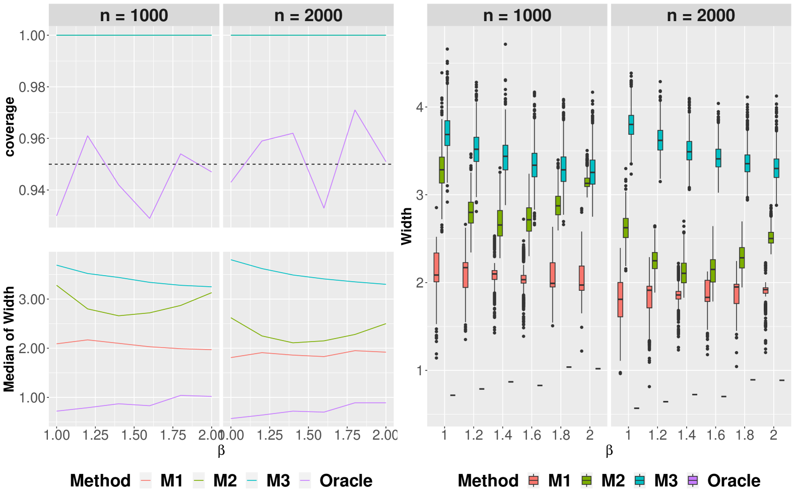
Figure 1: Comparison of coverage and width of various confidence sets of mode of $f_{\beta}$ for different sample sizes and smoothness parameter, $\beta$.

Figure 1 demonstrates the performance of the proposed finite sample valid confidence sets of mode of a unimodal distribution. It can be observed from the left panel of the figure that the finite sample valid methods (M1), (M2), (M3) are conservative and always provide the required coverage ($\geq 0.95$) for all sample sizes and all $\beta$ in contrast to the asymptotically valid oracle method. The “median of width” plot in the left panel and the box plot of width in the right panel reveal that the width of the confidence sets given by (M1) and (M2) gradually decrease as the sample size increases and approach the width of the oracle method. On the contrary, the width of the confidence set given by the p-value based method (M3) doesn’t seem to decrease with increasing sample size. All these observations align with the theoretical results discussed in the prior sections.

4 Conclusions and Future Directions

In this work, we address the problem of constructing finite-sample valid confidence sets for the mode of a unimodal distribution that shrink to a singleton as sample size increases—a task that has received comparatively little attention in the literature relative to point estimation. Building upon classical ideas, we introduce a suite of novel procedures that yield valid confidence sets under minimal assumptions. Our proposed methods leverage spacings between order statistics, M-estimation techniques, and single-observation-based inequalities [Edelman (1990)] to achieve finite-sample coverage guarantees. A salient feature of these procedures is their adaptivity to the underlying distribution: under suitable regularity conditions on the density around the mode, we show that the width of the confidence sets contracts at a rate that is minimax optimal (up to logarithmic factors), without requiring prior knowledge of the density’s smoothness.

Furthermore, we extend our framework to the multivariate setting by providing a generic methodology for obtaining finite-sample valid confidence sets for the mode of $\gamma$-unimodal distributions in $\mathbb{R}^{d}$, using algorithms developed for the univariate case as building blocks. Our theoretical results are complemented by numerical experiments on synthetic datasets. Collectively, our findings contribute new tools for inference on the mode and provide a foundation for future developments in finite-sample uncertainty quantification for statistical functionals.

There are various future directions to this work. Firstly, it is of interest to construct a less conservative finite sample valid confidence interval of the mode of a unimodal univariate distribution with coverage $1-\alpha$ and whose width shrinks to zero at exactly the minimax optimal rate as the sample size $n\rightarrow\infty$. Secondly, obtaining a finite sample analysis of the width of the confidence set of the mode of a multivariate $\gamma$-unimodal distribution [Algorithm 5] is also of interest.

Appendix to “Finite sample valid confidence sets of mode”

Appendix S.1 Finite sample valid confidence set of mode of dependent data

We often encounter scenarios where we can not assume the independence of data-points. There are various dependent structures which may occur – negatively associated (NA), negatively superadditive dependent (NSD), negatively orthant dependent (NOD), extended negatively dependent (END) etc. Refer to Joag-Dev and Proschan [1983], Hu [2000], Lehmann [2011], Liu [2009] for a more detailed discussion on these dependent structures. It can be shown that all these dependent structures mentioned above fall under the broader category of widely orthant dependent (WOD) data (Wang et al. [2013]). A given sequence of random variables $\{X_{N}\}_{N\geq 1}$ is said to be WOD with dominating coeffients $g(N)=\max\{g_{L}(N),g_{U}(N)\}$ if there exists sequences $\{g_{L}(N)\}_{N\geq 1},\{g_{U}(N)\}_{N\geq 1}\geq 1$ such that for any $x_{i}\in(-\infty,\infty),$ $i\leq N$,

$$\begin{split}\mathbb{P}(X_{1}>x_{1},\cdots,X_{N}>x_{N})&\leq g_{U}(N)\prod_{i=1}^{N}\mathbb{P}(X_{i}>x_{i}),\\ \mathbb{P}(X_{1}\leq x_{1},\cdots,X_{N}\leq x_{N})&\leq g_{L}(N)\prod_{i=1}^{N}\mathbb{P}(X_{i}\leq x_{i}).\end{split}$$

These dependent structures often arise in censored and truncated data which are very common in survival analysis, reliability theory, astronomy and economics. Kaber El Alem et al. [2024] is one of the papers which studies the consistency of the kernel mode estimator for truncated WOD data. In this section we leverage Edelman’s result (2) to construct a finite sample valid confidence set of the mode of a unimodal univarite distribution based on data which may have arbitrary dependency between the data-points. The method is described in Algorithm 6.

Input: Sample: $X_{1},\cdots,X_{m}$, Confidence Level: $1-\alpha$, tuning parameter $\rho>1$

Output: Confidence set for the population mode with finite sample coverage

1 Divide the sample into two almost equally sized disjoint sub-samples $S_{1}$ and $S_{2}$. Let $|S_{1}|=m-n$ and $|S_{2}|=n$.

2 Compute any consistent estimate $\widehat{\theta}_{1}$ of mode based on the sub-sample $S_{1}$.

Return the confidence set,

$$\widehat{\mathrm{CS}}_{n,\alpha}^{\mathrm{Ed}_{E},\rho}=\left\{\theta\in\mathbb{R}\Bigg{|}\frac{1}{n}\left(\frac{\rho-1}{\rho+1}\right)\sum_{i\in S_{2}}\left|\frac{X_{i}-\theta}{X_{i}-\widehat{\theta}_{1}}\right|^{1/\rho}<\frac{1}{\alpha}\right\}.$$

Algorithm 6 (M3’) Proposed finite sample valid confidence set for the population mode

Theorem 10.

Suppose $X_{1},\cdots,X_{m}$ are identically distributed as $F$ (density $f$) which is an absolutely continuous unimodal distribution with a unique mode $\theta_{0}$. Then the confidence set returned by Algorithm 4 satisfies the following for all $n\geq 1$, for any $\alpha\in(0,1)$ and for any $\rho>1$,

$$\mathbb{P}_{F}(\theta_{0}\in\widehat{\mathrm{CS}}_{n,\alpha}^{\mathrm{Ed}_{E},\rho})\geq 1-\alpha.$$

Proof of Theorem 10.

We use Edelman [1990]’s result that for any $t>1$ and any fixed $a\in\mathbb{R}$,

$$\mathbb{P}(|X-\theta_{0}|\leq t|X-a|)\geq 1-\frac{2}{t+1}.$$

Using this concentration around $\theta_{0}$ we can obtain a transformation $\psi(X)$ of $X$ which is bounded in $\mathcal{L}_{1}$. For any fixed $a\in\mathbb{R}$ we have,

$$\begin{split}\mathbb{E}\left[\left(\frac{\rho-1}{\rho+1}\right)\left|\frac{X-\theta_{0}}{X-a}\right|^{1/\rho}\right]&=\left(\frac{\rho-1}{\rho+1}\right)\mathbb{E}\left[\left|\frac{X-\theta_{0}}{X-a}\right|^{1/\rho}\right]\\ &=\left(\frac{\rho-1}{\rho+1}\right)\int_{0}^{\infty}\mathbb{P}\left(\left|\frac{X-\theta_{0}}{X-a}\right|^{1/\rho}>t\right)dt\\ &\leq\left(\frac{\rho-1}{\rho+1}\right)\left(1+\int_{1}^{\infty}\mathbb{P}\left(\left|\frac{X-\theta_{0}}{X-a}\right|>t^{\rho}\right)dt\right)\\ &\leq\left(\frac{\rho-1}{\rho+1}\right)\left(1+\int_{1}^{\infty}\frac{2}{t^{\rho}+1}dt\right)\\ &<\left(\frac{\rho-1}{\rho+1}\right)\left(1+\frac{2}{\rho-1}\right)\\ &=1.\end{split}$$

We use this $\mathcal{L}_{1}$ boundedness property to prove the coverage guarantee.

$$\begin{split}\mathbb{P}(\theta_{0}\notin\widehat{\mathrm{CS}}_{n,\alpha}^{\mathrm{Ed}_{E,\rho}})&=\mathbb{P}\left(\frac{1}{n}\left(\frac{\rho-1}{\rho+1}\right)\sum_{i\in S_{2}}\left|\frac{X_{i}-\theta_{0}}{X_{i}-\widehat{\theta}_{1}}\right|^{1/\rho}\geq\frac{1}{\alpha}\right)\\ &\stackrel{{\scriptstyle(i)}}{{\leq}}\alpha\mathbb{E}\left[\frac{1}{n}\left(\frac{\rho-1}{\rho+1}\right)\sum_{i\in S_{2}}\left|\frac{X_{i}-\theta_{0}}{X_{i}-\widehat{\theta}_{1}}\right|^{1/\rho}\right]\\ &=\alpha\mathbb{E}\left[\left(\frac{\rho-1}{\rho+1}\right)\left|\frac{X-\theta_{0}}{X-\widehat{\theta}_{1}}\right|^{1/\rho}\right]\\ &\stackrel{{\scriptstyle(ii)}}{{\leq}}\alpha.\end{split}$$

The step-$(i)$ follows because of Markov’s inequality. The step-$(ii)$ holds because of the $\mathcal{L}_{1}$ boundedness property of the transformed data (with $a=\widehat{\theta}_{1}$). This completes the proof of the theorem. ∎

In addition to being identically distributed, if the data $\{X_{i}\}_{i=1}^{m}$ are also independent, it can be shown that the confidence set converges almost surely to a limiting set as the sample size $m$ goes to infinity.

Theorem 11.

Suppose $X_{1},\cdots,X_{m}$ are independent and identically distributed as $F$ (density $f$) which is an absolutely continuous unimodal distribution with a unique mode $\theta_{0}$ such that $\mathbb{E}_{F}[|(X-\theta)/(X-\theta_{0})|^{1/\rho}]$ exists for all $\theta\in\mathbb{R}$. Let $\widehat{\theta}_{1}$ be a consistent estimator of $\theta_{0}$. Then we have,

$$\widehat{\mathrm{CS}}_{n,\alpha}^{\mathrm{Ed}_{E,\rho}}\stackrel{{\scriptstyle a.s.}}{{\rightarrow}}\left\{\theta\in\mathbb{R}\Bigg{|}\mathbb{E}_{F}\left[\left(\frac{\rho-1}{\rho+1}\right)\left|\frac{X-\theta}{X-\theta_{0}}\right|^{1/\rho}\right]<\frac{1}{\alpha}\right\}\quad\mbox{as}\quad m-n,n\rightarrow\infty,$$

Proof of Theorem 11.

The proof is a simple application of the law of large numbers. We have the following equivalence relation,

$$\begin{split}\theta\in\widehat{\mathrm{CS}}_{n,\alpha}^{\mathrm{Ed}_{E,\rho}}&\iff\left(\frac{\rho-1}{\rho+1}\right)\frac{1}{n}\sum_{i\in S_{2}}\left|\frac{X_{i}-\theta}{X_{i}-\widehat{\theta}_{1}}\right|^{1/\rho}<\frac{1}{\alpha}.\end{split}$$

As $n\rightarrow\infty$ the term in the left hand side converges almost surely to $((\rho-1)/(\rho+1))\mathbb{E}[|(X-\theta)/(X-\theta_{0})|^{1/\rho}]$ by strong law of large numbers (we also use the fact that $\widehat{\theta}_{1}$ is a consistent estimator of $\theta_{0}$). Thus as $m-n,n\rightarrow\infty$,

$$\widehat{\mathrm{CS}}_{n,\alpha}^{\mathrm{Ed}_{E,\rho}}\stackrel{{\scriptstyle a.s.}}{{\rightarrow}}\left\{\theta\in\mathbb{R}\Bigg{|}\mathbb{E}_{F}\left[\left(\frac{\rho-1}{\rho+1}\right)\left|\frac{X-\theta}{X-\theta_{0}}\right|^{1/\rho}\right]<\frac{1}{\alpha}\right\}$$

This completes the proof of the theorem. ∎

Appendix S.2 Proof of Theorem 1

We begin the proof by considering the following set of distribution functions,

$$\mathcal{C}_{n}(\alpha/2)=\left\{F:c_{B}\leq F(I_{Bi})\leq d_{B}\quad\mbox{for }i=1,\cdots,n_{B}\quad\mbox{and for }B=0,\cdots,B_{max}\right\},$$

where,

$$\begin{split}c_{B}&=q\mbox{Beta}(\alpha/(4(B+2)n_{B}t_{n}),2^{B+s_{n}},n+1-2^{B+s_{n}}),\\ d_{B}&=q\mbox{Beta}(1-(\alpha/(4(B+2)n_{B}t_{n})),2^{B+s_{n}},n+1-2^{B+s_{n}}).\end{split}$$

We know from Section $2.1$ of Walther et al. [2022] that,

$$\mathbb{P}_{F}(F\in\mathcal{C}_{n}(\alpha))\geq 1-(\alpha/2),$$ (E.1)

for any distribution function $F$. Our proof is based on the following fundamental property of unimodal distribution function, for two adjacent disjoint intervals $I_{1}=[a,b],I_{2}=[b,c]$ (where $-\infty<a<b<c<\infty$) if $F(I_{1})/|I_{1}|>F(I_{2})/|I_{2}|$ then either the mode $\theta_{0}\in I_{1}$ or $\theta_{0}<a$ i.e. the mode is ”closer” to the interval $I_{1}$ as compared to $I_{2}$. Thus we can drop $I_{2}$ and the intervals present after $I_{2}$ from the collection of intervals that can contain the mode. Similarly if $F(I_{1})/|I_{1}|<F(I_{2})/|I_{2}|$ then either the mode $\theta_{0}\in I_{2}$ or $\theta_{0}>c$ i.e. the mode is ”closer” to the interval $I_{2}$ as compared to $I_{1}$. Thus we can drop $I_{1}$ and the intervals present before $I_{1}$ from the collection of intervals that can contain the mode.

We note from the construction that for $0\leq B\leq B_{\max}$ the intervals $\{I_{Bi}\}_{i=1}^{n_{B}}$ are disjoint and every pair of consecutive intervals in this set share a common boundary. Moreover the intervals $\{I_{0i}\}_{i=1}^{n_{0}}$ are subsets of the intervals $\{I_{1i}\}_{i=1}^{n_{1}}$ which are in fact subsets of the intervals $\{I_{2i}\}_{i=1}^{n_{2}}$ and so on till $\{I_{B_{max}i}\}_{i=1}^{n_{B_{max}}}$. Using the fact that $\mathbb{P}_{F}(F\in\mathcal{C}_{n}(\alpha))\geq 1-(\alpha/2)$ we note that with probability greater than or equal to $1-(\alpha/2)$ the following holds for all $1\leq i\leq n_{B}$ and for all $0\leq B\leq B_{max}$,

$$\frac{c_{B}}{|I_{Bi}|}\leq\frac{F(I_{Bi})}{|I_{Bi}|}\leq\frac{d_{B}}{|I_{Bi}|}.$$ (E.2)

We start with $B=B_{max}$ and find the interval $I_{B_{max}i_{min}}$. By (E.2) $I_{B_{max}i_{min}}$ has the highest lower bound in the set $\{I_{B_{max}i}\}_{i=1}^{n_{B_{max}}}$. We now consider the set $K_{B_{max}}$. We observe that for all intervals $I_{B_{max}i}\in K_{B_{max}}$ the following holds,

$$\begin{split}&\mbox{Width}(I_{B_{max}i})\leq h_{B_{max}}\mbox{Width}(I_{B_{max}i_{min}})\\ \implies&|I_{B_{max}i}|\leq\frac{d_{B_{max}}}{c_{B_{max}}}|I_{B_{max}i_{min}}|\\ \implies&\frac{c_{B_{max}}}{|I_{B_{max}i_{min}}|}\leq\frac{d_{B_{max}}}{|I_{B_{max}i}|}.\end{split}$$

Thus $K_{B_{max}}$ comprises of the largest set of neighbouring intervals of $I_{B_{max}i_{min}}$ which have overlapping bounds with that of $I_{B_{max}i_{min}}$ i.e. $K_{B_{max}}$ consists of those intervals $I_{B_{max}i}$ for which the upper bound of $F(I_{B_{max}i})/|I_{B_{max}i}|$ is greater than the lower bound of $F(I_{B_{max}i_{min}})/|I_{B_{max}i_{min}}|$. From the fundamental property of unimodal distribution functions discussed before, we drop all the intervals in $\{I_{B_{max}i}\}_{i=1}^{n_{B_{max}}}$ which are not in the set $K_{B_{max}}$. Continuing like this for $B=B_{max}-1,\cdots,0$ we finally obtain $K_{0}$. By the same argument we know that the mode $\theta_{0}$ can not lie in any interval in the set $\cup_{i=1}^{n_{B_{0}}}\{I_{B_{0}i}\}\backslash K_{0}$. Thus either $\theta_{0}\in\left(-\infty,X_{(1)}\right]$ or $\theta_{0}\in K_{0}$ or $\theta_{0}\in\left[X_{(n)},\infty\right)$. However we know from the fundamental property of unimodal distribution functions that $\theta_{0}$ can lie in $\left(-\infty,X_{(1)}\right]$ iff the left most interval $I_{01}\in K_{0}$. Similarly we know that $\theta_{0}$ can lie in $\left[X_{(n)},\infty\right)$ iff the right most interval $I_{0n_{0}}\in K_{0}$.

Here we use Theorem-$4$ of Lanke [1974] which states that,

$$\mathbb{P}(\theta_{0}\in(X_{(1)}-\lambda_{n,\alpha}(X_{(n)}-X_{(1)}),X_{(n)}+\lambda_{n,\alpha}(X_{(n)}-X_{(1)})))\geq 1-(\alpha/2),$$ (E.3)

where $\lambda_{n,\alpha}$ is as described in Algorithm 1. Combining the previous discussion and the high probability statements in (E.1) and (E.3) we conclude that,

$$\mathbb{P}_{F}(\theta_{0}\in\widehat{\mathrm{CI}}_{n,\alpha})\geq(1-(\alpha/2))+(1-(\alpha/2))-1\geq 1-\alpha.$$

This completes the proof of the theorem.

Appendix S.3 Proof of Theorem 2

From Algorithm 1 we can see that $h_{B}$ is a decreasing function of $\alpha$. Thus because of the nested nature of the algorithm we have $\widehat{\mathrm{CI}}_{n,\alpha}\subset\widehat{\mathrm{CI}}_{n,1/n}$ and hence $\mathrm{Width}(\widehat{\mathrm{CI}}_{n,\alpha})\leq\mathrm{Width}(\widehat{\mathrm{CI}}_{n,1/n})$. Because of this it is enough to prove the theorem for $\alpha=1/n$. Therefore in the remaining proof we assume $\alpha=1/n$ without loss of generality. We note that the number of observations contained in $I_{Bi}$ is $2^{B+s_{n}}+1$ which varies from $\log(n)+1$ to $(n/8)+1$ as $B$ ranges from $0$ to $B_{max}$. Let $\log(n)<r(n)=An^{2\beta/(1+2\beta)}<n/8$ for some $A>0$ and let $0\leq B(r)=\log_{2}(r(n))-s_{n}\leq B_{\max}$. We note that the number of observations contained in $I_{B(r)i}$ is $r(n)+1$. We re-label the interval formed by the set $K_{B(r)+1}$ as $[c,d]$. If there are at-least $r(n)+1$ observations in $[c,d]$ we let $K(n)$ be the discrete random variable such that the following holds. $[X_{K(n)},X_{K(n)+r(n)}]=I_{B(r)i}$ for some $i$, $[X_{K(n)},X_{K(n)+r(n)}]\subset[c,d]$ and,

$$X_{K(n)+r(n)}-X_{K(n)}=\min\{\mbox{Width}(I_{B(r)i})|\mbox{ }I_{B(r)i}\subset[c,d]\}.$$

If $[c,d]$ does not contain $r(n)+1$ observations then $K(n)$ can be set to any arbitrary number (does not affect the proof). It is important to note that by definition $[X_{K(n)},X_{K(n)+r(n)}]=I_{B(r)i_{min}}$. Since $\widehat{\mathrm{CI}}_{n,\alpha}$ contains $\theta_{0}$ with probability at-least $1-(1/n)$ we have that $\theta_{0}\in[c,d]$ with probability at-least $1-(1/n)$. For showing the in probability convergence we can therefore do the remaining computations under the event $\{\theta_{0}\in[c,d]\}$. We also let $J(n)$ be the following discrete random variable. If $[\theta_{0},d]$ contains at-least $r(n)+1$ observations then we define $J(n)$ to be the smallest index $j$ such that $[X_{j},X_{j+r(n)}]=I_{B(r)i}$ for some $i$, $[X_{j},X_{j+r(n)}]\subset[\theta_{0},d]$. If $[\theta_{0},d]$ does not contain $r(n)+1$ observations then $J(n)$ can be set to any arbitrary number. We need the following lemma from Sager [1975].

Lemma 2.

Let $S_{1},S_{2},\cdots$ and $T_{1},T_{2},\cdots$ be a sequence of random variables such that $S_{n}\leq T_{n}$ for each $n$ and $[S_{n},T_{n}]$ contains $r(n)+1$ observations where $r(n)$ is of the form $An^{v}$, $0<v<1$. Then we have the following,

$$\frac{F(T_{n})-F(S_{n})}{F_{n}(T_{n})-F_{n}(S_{n})}=1+o(r(n)^{-1/2}log(r(n)))\quad\mbox{with probability one}.$$

We break the proof of the theorem into three cases. At first we prove the result for the case when $\theta_{0}=c$, then we prove the result for the case when $\theta_{0}=d$, and finally we prove for the case when $\theta_{0}\in(c,d)$.

Suppose $\theta_{0}=c$. We show that $X_{J(n)+r(n)}=c+o(\delta(n))$ with probability $1$ where $\delta(n)=n^{-1/(1+2\beta)}(\log n)^{1/\beta}$. We observe that $r^{+}(R_{2}\delta)\rightarrow f(c)$ as $\delta\rightarrow 0$. If this does not happen then we can say from the definition of $r^{+}(R_{2}(\delta)$ that for some $\epsilon>0$ and for all $c<x<d$ we have $f(x)+\epsilon<f(c)$. This implies that $f(c)+\epsilon<f(c)$, a contradiction to the assumption of standard conditions.

Combining the above with the fact that $r(\delta,R_{2}\delta)\geq 1+\rho\delta^{\beta}$ we can say that there exists a constant $B>0$ such that $B<r^{+}(R_{2}\delta)<r^{-}(\delta)\leq r^{-}(\epsilon\delta)$ for all small $\delta$ and for each $0<\epsilon<1$. Thus for $0<\epsilon<1$ and for all large $n$ the following holds true,

$$F(c+\epsilon\delta_{n})-F(c)\geq\int_{c}^{c+\epsilon\delta_{n}}r^{-}(\epsilon\delta(n))dx>B\epsilon\delta(n).$$

This implies that,

$$\liminf_{n\rightarrow\infty}\frac{F(c+\epsilon\delta(n))-F(c)}{B\epsilon\delta(n)}\geq 1.$$ (E.4)

On the other hane using Lemma 2 and the definition of $J(n)$ we get that,

$$1\leq\liminf_{n\rightarrow\infty}\frac{F(X_{J(n)+r(n)})-F(c)}{r(n)/n}\leq\limsup_{n\rightarrow\infty}\frac{F(X_{J(n)+r(n)})-F(c)}{r(n)/n}\leq 2\mbox{ with probability }1.$$

We note that $n^{-1}r(n)/(B\epsilon\delta(n))\rightarrow 0$ as $n\rightarrow\infty$. Using this in the previous equation we obtain that,

$$\lim_{n\rightarrow\infty}\frac{F(X_{J(n)+r(n)})-F(c)}{B\epsilon\delta(n)}\rightarrow 0\mbox{ with probability }1.$$ (E.5)

The equations (E.4) and (E.5) imply that $F(c+\epsilon\delta(n))>F(X_{J(n)+r(n)})$ with probability $1$. Since $\epsilon$ can be chosen arbitrarily we conclude that $X_{J(n)+r(n)}=c+o(\delta(n))$ with probability $1$.

Suppose $L(n)$ is the discrete random variable such that $[X_{L(n)},X_{L(n)+r(n)}]=I_{B(r)i_{ex}}\subset K_{B(r)}$ where $I_{B(r)i_{ex}}$ is the right extreme interval present in the set $K_{B(r)}$. Analysis can be similarly done for the left extreme interval present in the set $K_{B(r)}$. We show that $X_{L(n)}=c+o(\delta(n))$ with probability $1$. From Algorithm 1 we know that,

$$\frac{X_{L(n)+r(n)}-X_{L(n)}}{X_{K(n)+r(n)}-X_{K(n)}}\leq h_{B(r)}=\frac{d_{B(r)}}{c_{B(r)}}.$$

Here we use a result from Hengartner and Stark [1995]. Suppose $\tau$ is a constant such that,

$$2\beta+\frac{2\tau^{3}}{3}\sqrt{\frac{\log(n)}{(1+2\beta)n^{2\beta/(1+2\beta)}}}\leq\tau^{2}-2.$$

Then the following holds true,

$$\begin{split}\lim_{n\rightarrow\infty}\left(c_{B(r(n))}-\frac{r(n)-\sqrt{r(n)}\tau\sqrt{\log(n/r(n))}}{n+\sqrt{n}z_{1-\alpha/2}}\right)&\geq 0\\ \lim_{n\rightarrow\infty}\left(d_{B(r(n))}-\frac{r(n)+\sqrt{r(n)}\tau\sqrt{\log(n/r(n))}}{n-\sqrt{n}z_{1-\alpha/2}}\right)&\leq 0.\end{split}$$

We now analyze the behavior of $h_{B(r)}$. All the inequalities in the following equation are true upto a constant.

$$\begin{split}h_{B(r(n))}&=\frac{d_{B(r(n))}}{c_{B(r(n))}}\\ &\leq\frac{r(n)+\sqrt{r(n)}\tau\sqrt{\log(n/r(n))}}{n-\sqrt{n}z_{1-\alpha/2}}\frac{n+\sqrt{n}z_{1-\alpha/2}}{r(n)-\sqrt{r(n)}\tau\sqrt{\log(n/r(n))}}\\ &=\frac{n^{2\beta/(1+2\beta)}+n^{\beta/(1+2\beta)\sqrt{\log(n^{1/(1+2\beta)})}}}{n^{2\beta/(1+2\beta)}-n^{\beta/(1+2\beta)\sqrt{\log(n^{1/(1+2\beta)})}}}\frac{n+\sqrt{n}z_{1-\alpha/2}}{n-\sqrt{n}z_{1-\alpha/2}}\\ &=\left(1+\frac{1}{n^{\beta/(1+2\beta)}(\log n)^{-1/2}}\right)\left(1+o(n^{-1/2})\right)\\ &=(1+o(n^{-\beta/(1+2\beta)}\log(n)))(1+o(n^{-1/2}))\\ &=1+o(n^{-\beta/(1+2\beta)}\log(n)).\end{split}$$

Suppose $\Omega_{L}$ is the set where our claim that $X_{L(n)}=c+o(\delta(n))$ with probability $1$ does not hold true. If $\omega\in\Omega_{L}$, there exists a subsequence $\{n(j)\}$ and and $\epsilon$ such that $X_{L(n(j))}>c+R_{2}\epsilon\delta(n(j))$ for all $j$.

Setting $S_{n}=X_{L(n)},T_{n}=X_{L(n)+r(n)}$ and $S_{n}=X_{J(n)},T_{n}=X_{J(n)+r(n)}$ and using Lemma 2 we get that the following holds with probability $1$,

$$\begin{split}\frac{F(X_{L(n)+r(n)})-F(X_{L(n)})}{r(n)/n}&=1+o(r(n)^{-1/2}\log(r(n))),\\ \frac{F(X_{J(n)+r(n)})-F(X_{J(n)})}{r(n)/n}&=1+o(r(n)^{-1/2}\log(r(n))).\end{split}$$

Using the assumption made in Theorem 2 we have,

$$\begin{split}1+\rho(\epsilon\delta(n(j)))^{\beta}&\leq r(\epsilon\delta(n(j)),R_{2}\epsilon\delta(n(j)))\\ &\leq\frac{r^{-}(\epsilon\delta(n(j)))}{r^{+}(R_{2}\epsilon\delta(n(j)))}\frac{X_{J(n(j))+r(n(j))}-X_{J(n(j))}}{X_{K(n(j))+r(n(j))}-X_{K(n(j))}}\\ &\leq\frac{r^{-}(\epsilon\delta(n(j)))}{r^{+}(R_{2}\epsilon\delta(n(j)))}\frac{X_{J(n(j))+r(n(j))}-X_{J(n(j))}}{X_{L(n(j))+r(n(j))}-X_{L(n(j))}}h_{B(r(n(j)))}\\ &\leq\frac{(F(X_{J(n(j))+r(n(j))})-F(X_{J(n(j))}))}{(F(X_{L(n(j))+r(n(j))})-F(X_{L(n(j))}))}\frac{n(j)r(n(j))^{-1}}{n(j)r(n(j))^{-1}}h_{B(r(n(j)))}\\ &\leq(1+o(r(n(j))^{-1/2}\log(r(n(j)))))(1+o(n(j)^{-\beta/(1+2\beta)}\log(n(j))))\\ &=(1+o(n(j)^{-\beta/(1+2\beta)}\log(n(j))))(1+o(n(j)^{-k/(1+2k)}\log(n(j))))\\ &=(1+o(n(j)^{-\beta/(1+2\beta)}\log(n(j)))).\end{split}$$

This is a contradiction because $1+\rho(\epsilon\delta(n(j)))^{\beta}=1+\rho\epsilon^{\beta}n(j)^{-\beta/(1+2\beta)}\log(n(j))$ and this violates the above inequality for large $j$. Thus we conclude that $X_{L(n)}=c+o(\delta(n))$ with probability $1$. Moreover with probability $1$ we also have,

$$\begin{split}X_{L(n)+r(n)}-c&=(X_{L(n)+r(n)}-X_{L(n)})+X_{L(n)}-c\\ &\leq h_{B(r(n))}(X_{K(n)+r(n)}-X_{K(n)})+X_{L(n)}-c\\ &\leq h_{B(r(n))}(X_{J(n)+r(n)}-X_{J(n)})+X_{L(n)}-c\\ &\leq(1+o(\delta(n)^{\beta}))o(\delta(n))+o(\delta(n))\\ &=o(\delta(n)).\end{split}$$

In the above we use the fact that $h_{B(r(n))}\leq 1+o(n^{-\beta/(1+2\beta)}\log(n))=1+o(\delta(n)^{\beta})$, $(X_{J(n)+r(n)}-X_{J(n)})\leq(X_{J(n)+r(n)}-c)=o(\delta(n))$, and $X_{L(n)}-c=o(\delta(n))$. We note that $\widehat{\mathrm{CI}}_{n,\alpha}\subset K_{B(r)}$ and $X_{L(n)+r(n)}$ is the right end-point of the confidence interval formed by $K_{B(r)}$. A similar result can be obtained for the left end-point of the confidence interval formed by $K_{B(r)}$. Since both the end-points behave as $c+o(\delta(n))$, the width of the confidence interval formed by $K_{B(r)}$ and thus also $\mbox{Width}(\widehat{\mathrm{CI}}_{n,\alpha})$ behaves as $o(\delta(n))$. This completes the proof for the case when $\theta_{0}=c$. The proof for the case when $\theta_{0}=d$ is similar.

Now suppose $\theta_{0}\in(c,d)$. We define discrete random variables $K_{1}(n)$ and $K_{2}(n)$ as follows. $[X_{K_{1}(n)},X_{K_{1}(n)+r(n)}]=I_{B(r)i}$ for some $i$, $[X_{K_{1}(n)},X_{K_{1}(n)+r(n)}]\subset[c,\theta_{0}]$ and,

$$X_{K_{1}(n)+r(n)}-X_{K_{1}(n)}=\min\{\mbox{Width}(I_{B(r)i})|I_{B(r)i}\subset[c,\theta_{0}]\}.$$

Similarly $[X_{K_{2}(n)},X_{K_{2}(n)+r(n)}]=I_{B(r)i}$ for some $i$, $[X_{K_{2}(n)},X_{K_{2}(n)+r(n)}]\subset[\theta_{0},d]$ and,

$$X_{K_{2}(n)+r(n)}-X_{K_{2}(n)}=\min\{\mbox{Width}(I_{B(r)i})|I_{B(r)i}\subset[\theta_{0},d]\}.$$

Suppose $L_{1}(n)$ and $L_{2}(n)$ are discrete random variables such that $[X_{L_{1}(n)},X_{L_{1}(n)+r(n)}]=I_{B(r)i}\mbox{ (for some $i$) }\subset[c,\theta_{0}]$, $[X_{L_{2}(n)},X_{L_{2}(n)+r(n)}]=I_{B(r)i}\mbox{ (for some $i$) }\subset[\theta_{0},d]$ and,

$$\begin{split}\frac{X_{L_{1}(n)+r(n)}-X_{L_{1}(n)}}{X_{K_{1}(n)+r(n)}-X_{K_{1}(n)}}&\leq h_{B(r(n))},\\ \frac{X_{L_{2}(n)+r(n)}-X_{L_{2}(n)}}{X_{K_{2}(n)+r(n)}-X_{K_{2}(n)}}&\leq h_{B(r(n))}.\end{split}$$

From the previous cases we know that $X_{L_{1}(n)}=c+o(\delta(n))$ and $X_{L_{2}(n)+r(n)}=c+o(\delta(n))$ with probability $1$. We observe that $\widehat{\mathrm{CI}}_{n,\alpha}\subset\mbox{ C.I. generated by }K_{B(r(n))}\subset[X_{L_{1}(n)},X_{L_{2}(n)+r(n)}]$. Thus we have $\mbox{Width}(\widehat{\mathrm{CI}}_{n,\alpha})\leq X_{L_{2}(n)+r(n)}-X_{L_{1}(n)}=o(\delta(n))$ with probability $1$. In other words $n^{1/(1+2\beta)}(\log n)^{-1/\beta}\mbox{Width}(\widehat{\mathrm{CI}}_{n,\alpha})\stackrel{{\scriptstyle P}}{{\rightarrow}}0$ as $n\rightarrow\infty$. This completes the proof of the theorem.

Appendix S.4 Proof of Theorem 3

We note that $\theta_{0}=\mbox{arg max}_{x}(f(x))$. Let $g_{h}$ be the density of a Uniform$[-h,h]$ random variable. We consider the convolution $f*g_{h}$,

$$\begin{split}f*g_{h}(y)&=\int_{-h}^{h}f(y-x)g_{h}(x)dx\\ &=\frac{1}{2h}\int_{-h}^{h}f(y-x)dx\\ &=\frac{F(y+h)-F(y-h)}{2h}\\ &=\mathbb{E}\left[\frac{1}{2h}\textbf{1}\{y-h<X\leq y+h\}\right].\end{split}$$

Let $F_{h}$ be the corresponding distribution function of the convolution $f*g_{h}$. Let $\theta_{h}=\mbox{arg max}_{y}(f*g_{h}(y))$ be the population mode of the convolution $f*g_{h}$. We note the following characterization of $\theta_{h}$,

$$\begin{split}\theta_{h}&=\mbox{arg min}_{y}(-f*g_{h}(y))\\ &=\mbox{arg min}_{y}\mathbb{E}\left[-\frac{1}{2h}\textbf{1}\{y-h<X\leq y+h\}\right]\\ &=\mbox{arg min}_{y}Pm_{y;h},\end{split}$$

where $m_{y;h}$ is as defined in Algorithm 2. We further observe the following for $y\geq\theta_{0}+h$,

$$\begin{split}f*g_{h}(y)&=\int_{-h}^{h}f(y-x)g_{h}(x)dx\\ &\leq\int_{-h}^{h}f(\theta_{0}+h-x)g_{h}(x)dx\\ &=f*g_{h}(\theta_{0}+h).\end{split}$$

We can similarly show that $f*g_{h}(y)\leq f*g_{h}(\theta_{0}-h)$ if $y\leq\theta_{0}-h$. Thus the mode of the convolution, $\theta_{h}=\mbox{arg max}_{y}(f*g_{h}(y))\in(\theta_{0}-h,\theta_{0}+h)$. This implies that,

$$\theta_{0}\in(\theta_{h}-h,\theta_{h}+h).$$ (E.6)

This suggests that if we can compute a finite sample valid $(1-\alpha)$ confidence set $\tilde{\mathrm{CI}}_{n,\alpha}^{h}$ of $\theta_{h}$, then $\tilde{\mathrm{CI}}_{n,\alpha}^{h}\pm h$ will be a finite sample valid $(1-\alpha)$ confidence set of $\theta_{0}$. From Theorem-$2$ in Takatsu and Kuchibhotla [2025] we see that if we can find a random mapping $\theta\rightarrow L_{n,\alpha}(\theta,\widehat{\theta}_{1};S_{2})=P_{n}(m_{\theta;h}-m_{\widehat{\theta}_{1};h})-t(\alpha,\theta,\widehat{\theta}_{1})$ (for some non-negative function $t(\cdot,\cdot,\cdot)$) such that,

$$\mathbb{P}(P(m_{\theta_{h};h}-m_{\widehat{\theta}_{1};h})\geq L_{n,\alpha}(\theta,\widehat{\theta}_{1};S_{2})|S_{1})=\mathbb{P}((P_{n}-P)(m_{\theta_{h};h}-m_{\widehat{\theta}_{1};h})\leq t(\alpha,\theta_{h},\widehat{\theta}_{1})|S_{1})\geq 1-\alpha,$$ (E.7)

then $\tilde{\mathrm{CI}}_{n,\alpha}^{h}=\{\theta\in\mathbb{R}|L_{n,\alpha}(\theta,\widehat{\theta}_{1};S_{2})\leq 0\}$ is a finite sample valid $(1-\alpha)$ confidence set of $\theta_{h}$.

We note that $(m_{\theta_{h};h}-m_{\widehat{\theta}_{1};h})(X)$ is a trinomial distribution that takes value $-1/2h,0,1/2h$. We use the following one-sided concentration inequality for the mean of trinomial distribution.

Lemma 3.

Let $Z_{1},\cdots,Z_{n}$ be iid random variables from a trinomial distribution which takes values $t_{1},t_{2},t_{3}$ with probabilities $p,q,1-p-q$ respectively. Let $\mu$ and $\widehat{\mu}$ be the population mean and sample mean respectively. Then for $\alpha\in(0,1)$ we have,

$$\mathbb{P}\left(\widehat{\mu}-\mu\leq(|t_{1}|+|t_{2}|+|t_{3}|)\sqrt{\frac{3}{2n}}\left[\sqrt{\log(1/\alpha)}+2\right]\right)\geq 1-\alpha.$$

Using Lemma 3 with $(t_{1},t_{2},t_{3})=(-1/2h,0,1/2h)$ we get that $t(\alpha,\theta_{h},\widehat{\theta}_{1})=\sqrt{3/(2n)}(1/h)[\sqrt{\log(1/\alpha)}+2]$ satisfies the condition (E.7). Hence,

$$\begin{split}\widehat{\mathrm{CS}}_{n,\alpha}^{h}&=\tilde{\mathrm{CS}}_{n,\alpha}^{h}\pm h\\ &=\{\theta\in\mathbb{R}|L_{n,\alpha}(\theta,\widehat{\theta}_{1};S_{2})\leq 0\}\pm h\\ &=\{\theta\in\mathbb{R}|P_{n}(m_{\theta;h}-m_{\widehat{\theta}_{1};h})\leq t(\alpha,\theta,\widehat{\theta}_{1})\}\pm h\\ &=\left\{\theta\in\mathbb{R}\Bigg{|}P_{n}(m_{\theta;h}-m_{\widehat{\theta}_{1};h})\leq\frac{1}{h}\sqrt{\frac{3}{2n}}\left[\sqrt{\log(1/\alpha)}+2\right]\right\}\pm h\end{split}$$

is a finite sample $(1-\alpha)$ confidence set of $\theta_{0}$. This complete the proof of the theorem.

We now provide a proof of Lemma 3.

Proof of Lemma 3.

Let $p_{n}=P_{n}I(Z_{i}=t_{1}),q_{n}=P_{n}I(Z_{i}=t_{2})$ be the sample estimates of $p,q$ respectively. Let $Q,Q_{n}$ be the trinomial distributions which take values $t_{1},t_{2},t_{3}$ with probabilities $p,q,1-p-q$ and $p_{n},q_{n},1-p_{n}-q_{n}$ respectively. For any $\epsilon>0$ we have the following,

$$\begin{split}&\mathbb{P}\left(\widehat{\mu}-\mu\leq(|t_{1}|+|t_{2}|+|t_{3}|)\epsilon\right)\\ \geq&\mathbb{P}\left(|\widehat{\mu}-\mu|\leq(|t_{1}|+|t_{2}|+|t_{3}|)\epsilon\right)\\ =&\mathbb{P}\left(|(p_{n}-p)t_{1}+(q_{n}-q)t_{2}+(p+q-p_{n}-q_{n})t_{3}|\leq(|t_{1}|+|t_{2}|+|t_{3}|)\epsilon\right)\\ \geq&\mathbb{P}(\delta(Q_{n},Q)\leq\epsilon)\\ \stackrel{{\scriptstyle(i)}}{{\geq}}&\mathbb{P}(\sqrt{(1/2)KL(Q_{n}||Q)}\leq\epsilon)\\ =&\mathbb{P}(KL(Q_{n}||Q)\leq 2\epsilon^{2})\\ \stackrel{{\scriptstyle(ii)}}{{\geq}}&1-\exp(-2n\epsilon^{2})\left(e\epsilon^{2}n\right)^{2}.\end{split}$$

Here $\delta(Q_{n},Q)=\sup\{|Q_{n}(A)-Q(A)|:A\mbox{ is measurable}\}$ is the total variation distance between $Q_{n}$ and $Q$ and $KL(Q_{n},Q)$ is the Kullback-Leibler divergence between $Q_{n}$ and $Q$. In step-$(i)$ we use the Pinsker’s inequality [Reid and Williamson [2009]] that $\delta(Q_{n},Q)\leq\sqrt{(1/2)KL(Q_{n},Q)}$. In step-(ii) we use Theorem-$1.2$ of Agrawal [2020] with $k=3$. We now observe that for $\epsilon^{2}=(3/(2n))\log(9e^{2}/(2\alpha))$ we have,

$$\begin{split}\exp(-2n\epsilon^{2})\left(e\epsilon^{2}n\right)^{2}&=\left(\frac{2\alpha}{9e^{2}}\right)^{3}\left(\frac{3e}{2}\right)^{2}\log^{2}\left(9e^{2}/(2\alpha)\right)\\ &\stackrel{{\scriptstyle(i)}}{{\leq}}\left(\frac{3e}{2}\right)^{2}\left(\frac{2\alpha}{9e^{2}}\right)^{3}\left(1-2\frac{9e^{2}}{2\alpha}+\left(\frac{9e^{2}}{2\alpha}\right)^{2}\right)\\ &\leq\left(\frac{3e}{2}\right)^{2}\frac{4\alpha}{9e^{2}}\\ &\leq\alpha.\end{split}$$

In step-$(i)$ we use $\log(1+x)<x$ for $x>0$. Therefore we see that with probability at-least $1-\alpha$,

$$\begin{split}\widehat{\mu}-\mu&\leq(|t_{1}|+|t_{2}|+|t_{3}|)\sqrt{\frac{3}{2n}}\sqrt{\log\left(\frac{9e^{2}}{2\alpha}\right)}\\ &\leq(|t_{1}|+|t_{2}|+|t_{3}|)\sqrt{\frac{3}{2n}}\left[\sqrt{\log(1/\alpha)}+\sqrt{\log\left(\frac{9e^{2}}{2}\right)}\right]\\ &\leq(|t_{1}|+|t_{2}|+|t_{3}|)\sqrt{\frac{3}{2n}}\left[\sqrt{\log(1/\alpha)}+2\right].\end{split}$$

This completes the proof of the lemma. ∎

Appendix S.5 Proof of Theorem 4

In this proof we redefine $m_{\theta;h}(X)=-\textbf{1}\{\theta-h<X\leq\theta+h\}$. Thus the confidence set $\widehat{\mathrm{CS}}_{n,\alpha}^{h}$ returned by the algorithm becomes,

$$\widehat{\mathrm{CS}}_{n,\alpha}^{h}=\left\{\theta\in\mathbb{R}\Bigg{|}P_{n}(m_{\theta;h}-m_{\widehat{\theta}_{1};h})\leq\sqrt{\frac{6}{n}}\left[\sqrt{\log(1/\alpha)}+2\right]\right\}\pm h=\tilde{\mathrm{CS}}_{n,\alpha}^{h}\pm h.$$

The confidence set $\tilde{\mathrm{CS}}_{n,\alpha}^{h}$ is contained $P-$almost surely in the following sets,

$$\begin{split}\tilde{\mathrm{CS}}_{n,\alpha}^{h}=&\left\{\theta\in\mathbb{R}\Bigg{|}P_{n}(m_{\theta;h}-m_{\widehat{\theta}_{1};h})\leq\sqrt{\frac{6}{n}}\left[\sqrt{\log(1/\alpha)}+2\right]\right\}\\ \subseteq&\left\{\theta\in\mathbb{R}\Bigg{|}P_{n}(m_{\theta;h}-m_{\theta_{0};h})\leq\sqrt{\frac{6}{n}}\left[\sqrt{\log(1/\alpha)}+2\right]+|P_{n}(m_{\widehat{\theta}_{1};h}-m_{\theta_{0};h})|\right\}\\ \subseteq&\left\{\theta\in\mathbb{R}\Bigg{|}P(m_{\theta;h}-m_{\theta_{0};h})\leq-n^{-1/2}G_{n}(m_{\theta;h}-m_{\theta_{0};h})+\Gamma_{n}(\widehat{\theta}_{1},\theta_{0})\right\}\\ \subseteq&\left\{\theta\in\mathbb{R}\Bigg{|}|\theta-\theta_{0}|\leq\left\{\left(\frac{4C_{0}}{(\beta+1)c_{0}}\right)^{1/\beta}+1\right\}h\right\}\\ &\bigcup\left\{\theta\in\mathbb{R}\Bigg{|}|\theta-\theta_{0}|>\left\{\left(\frac{4C_{0}}{(\beta+1)c_{0}}\right)^{1/\beta}+1\right\}h;\mbox{ }P(m_{\theta;h}-m_{\theta_{0};h})\leq-n^{-1/2}G_{n}(m_{\theta;h}-m_{\theta_{0};h})+\Gamma_{n}(\widehat{\theta}_{1},\theta_{0})\right\},\end{split}$$

where $\Gamma_{n}(\widehat{\theta}_{1},\theta_{0})=\sqrt{6/n}[\sqrt{\log(1/\alpha)}+2]+|P_{n}(m_{\widehat{\theta}_{1};h}-m_{\theta_{0};h})|$. We observe that,

$$P(m_{\theta;h}-m_{\theta_{0};h})=\{F(\theta_{0}+h)-F(\theta_{0}-h)\}-\{F(\theta+h)-F(\theta-h)\}.$$ (E.8)

We use assumption 1 to lower bound $P(m_{\theta;h}-m_{\theta_{0};h})$ for $|\theta-\theta_{0}|>((4C_{0}/((\beta+1)c_{0}))^{1/\beta}+1)h$. We note that,

$$\begin{split}F(\theta_{0}+h)-F(\theta_{0}-h)&\geq 2\int_{0}^{h}(f(\theta_{0})-C_{0}x^{\beta})dx\\ &=2h\left(f(\theta_{0})-\frac{C_{0}h^{\beta}}{\beta+1}\right).\end{split}$$

For $((4C_{0}/((\beta+1)c_{0}))^{1/\beta}+1)h\leq|\theta-\theta_{0}|\leq h_{0}-h$ we have,

$$\begin{split}F(\theta+h)-F(\theta-h)&\leq\int_{|\theta-\theta_{0}|-h}^{|\theta-\theta_{0}|+h}(f(\theta_{0})-c_{0}x^{\beta})dx\\ &=f(\theta_{0}).2h-c_{0}\frac{(|\theta-\theta_{0}|+h)^{\beta+1}-(|\theta-\theta_{0}|-h)^{\beta+1}}{\beta+1}\\ &\leq f(\theta_{0}).2h-c_{0}\frac{(\beta+1)|\theta-\theta_{0}|^{\beta}h}{\beta+1}\\ &=2h\left(f(\theta_{0})-(c_{0}/2)|\theta-\theta_{0}|^{\beta}\right).\end{split}$$

Hence for $((4C_{0}/((\beta+1)c_{0}))^{1/\beta}+1)h\leq|\theta-\theta_{0}|\leq h_{0}-h$ we have,

$$\begin{split}P(m_{\theta;h}-m_{\theta_{0};h})=&\{F(\theta_{0}+h)-F(\theta_{0}-h)\}-\{F(\theta+h)-F(\theta-h)\}\\ \geq&2h\left(f(\theta_{0})-\frac{C_{0}h^{\beta}}{\beta+1}\right)-2h\left(f(\theta_{0})-(c_{0}/2)|\theta-\theta_{0}|^{\beta}\right)\\ =&2h\left((c_{0}/2)|\theta-\theta_{0}|^{\beta}-\frac{C_{0}h^{\beta}}{\beta+1}\right)\\ \stackrel{{\scriptstyle(i)}}{{\geq}}&\frac{hc_{0}}{2}|\theta-\theta_{0}|^{\beta}.\end{split}$$

The condition $((4C_{0}/((\beta+1)c_{0}))^{1/\beta}+1)h\leq|\theta-\theta_{0}|$ implies that $C_{0}h^{\beta}/(\beta+1)\leq(c_{0}/4)|\theta-\theta_{0}|^{\beta}$ which justifies step-$(i)$. We now consider $\theta$ such that $h_{0}-h<|\theta-\theta_{0}|\leq h_{0}+h$.

$$\begin{split}F(\theta+h)-F(\theta-h)&\leq\int_{|\theta-\theta_{0}|-h}^{h_{0}}(f(\theta_{0})-c_{0}x^{\beta})dx+(f(\theta_{0})-c_{0}h_{0}^{\beta})(|\theta-\theta_{0}|+h-h_{0})\\ &=f(\theta_{0})2h-c_{0}\left\{\frac{h_{0}^{\beta+1}-(|\theta-\theta_{0}|-h)^{\beta+1}}{\beta+1}+h_{0}^{\beta}(|\theta-\theta_{0}|+h-h_{0})\right\}\\ &\leq f(\theta_{0})2h-c_{0}\left\{(|\theta-\theta_{0}|-h)^{\beta}(h_{0}-|\theta-\theta_{0}|+h)+h_{0}^{\beta}(|\theta-\theta_{0}|+h-h_{0})\right\}\\ &\leq 2h\left(f(\theta_{0})-c_{0}(|\theta-\theta_{0}|-h)^{\beta}\right)\\ &\leq 2h\left(f(\theta_{0})-c_{0}(h_{0}-2h)^{\beta}\right).\end{split}$$

Moreover if $|\theta-\theta_{0}|>h_{0}+h$ then,

$$F(\theta+h)-F(\theta-h)\leq 2h\left(f(\theta_{0})-c_{0}h_{0}^{\beta}\right).$$

Thus combining the above two inequalities we have for any $\theta$ such that $|\theta-\theta_{0}|>h_{0}-h$,

$$\begin{split}P(m_{\theta;h}-m_{\theta_{0};h})=&\{F(\theta_{0}+h)-F(\theta_{0}-h)\}-\{F(\theta+h)-F(\theta-h)\}\\ \geq&2h\left(f(\theta_{0})-\frac{C_{0}h^{\beta}}{\beta+1}\right)-2h\left(f(\theta_{0})-c_{0}(h_{0}-2h)^{\beta}\right)\\ =&2h\left(c_{0}(h_{0}-2h)^{\beta}-\frac{C_{0}h^{\beta}}{\beta+1}\right).\end{split}$$

These results imply that $P-$almost surely the confidence set $\tilde{\mathrm{CS}}_{n,\alpha}^{h}$ is contained in,

$$\begin{split}\tilde{\mathrm{CS}}_{n,\alpha}^{h}\subseteq&\left\{\theta\in\mathbb{R}\Bigg{|}|\theta-\theta_{0}|\leq\left\{\left(\frac{4C_{0}}{(\beta+1)c_{0}}\right)^{1/\beta}+1\right\}h\right\}\\ &\bigcup\left\{\theta\in\mathbb{R}\Bigg{|}|\theta-\theta_{0}|>\left\{\left(\frac{4C_{0}}{(\beta+1)c_{0}}\right)^{1/\beta}+1\right\}h;\mbox{ }P(m_{\theta;h}-m_{\theta_{0};h})\leq-n^{-1/2}G_{n}(m_{\theta;h}-m_{\theta_{0};h})+\Gamma_{n}(\widehat{\theta}_{1},\theta_{0})\right\}\\ \subseteq&\left\{\theta\in\mathbb{R}\Bigg{|}|\theta-\theta_{0}|\leq\left\{\left(\frac{4C_{0}}{(\beta+1)c_{0}}\right)^{1/\beta}+1\right\}h\right\}\\ &\bigcup\left\{\theta\in\mathbb{R}\Bigg{|}\left\{\left(\frac{4C_{0}}{(\beta+1)c_{0}}\right)^{1/\beta}+1\right\}h<|\theta-\theta_{0}|\leq h_{0}-h;\mbox{ }\frac{hc_{0}}{2}|\theta-\theta_{0}|^{\beta}\leq-n^{-1/2}G_{n}(m_{\theta;h}-m_{\theta_{0};h})+\Gamma_{n}(\widehat{\theta}_{1},\theta_{0})\right\}\\ &\bigcup\left\{\theta\in\mathbb{R}\Bigg{|}|\theta-\theta_{0}|>h_{0}-h;\mbox{ }2h\left(c_{0}(h_{0}-2h)^{\beta}-\frac{C_{0}h^{\beta}}{\beta+1}\right)\leq-n^{-1/2}G_{n}(m_{\theta;h}-m_{\theta_{0};h})+\Gamma_{n}(\widehat{\theta}_{1},\theta_{0})\right\}\\ \coloneqq&\mathbf{I}\cup\mathbf{II}\cup\mathbf{III}.\end{split}$$

We now derive a bound for $\mathbb{E}[\sup_{|\theta-\theta_{0}|<\delta}|G_{n}(m_{\theta;h}-m_{\theta_{0};h})|]=\mathbb{E}[\sup_{m\in M_{\theta_{0},\delta,h}}|G_{n}m|]$ where $M_{\theta_{0},\delta,h}=\{m_{\theta;h}-m_{\theta_{0};h}||\theta-\theta_{0}|<\delta\}$ and $0<\delta<h$. $M_{\theta_{0},\delta,h}$ is equipped with envelope function $F=1$. Moreover for $m=m_{\theta;h}-m_{\theta_{0};h}\in M_{\theta_{0},\delta,h}$ we have,

$$\begin{split}\mathbb{E}[m^{2}]=&\mathbb{E}(m_{\theta;h}-m_{\theta_{0};h})^{2}\\ =&F[[\theta-h,\theta+h]\cap[\theta_{0}-h,\theta_{0}+h]^{c}]+F[[\theta-h,\theta+h]^{c}\cap[\theta_{0}-h,\theta_{0}+h]]\\ \leq&\int_{\theta_{0}+h}^{\theta_{0}+h+\delta}(f(\theta_{0})-c_{0}x^{\beta})dx+\int_{\theta_{0}-h}^{\theta_{0}-h+\delta}(f(\theta_{0})-c_{0}x^{\beta})dx\\ =&f(\theta_{0})\delta-c_{0}\frac{(\theta_{0}+h+\delta)^{\beta+1}-(\theta_{0}+h)^{\beta+1}}{\beta+1}+f(\theta_{0})\delta-c_{0}\frac{(\theta_{0}-h+\delta)^{\beta+1}-(\theta_{0}-h)^{\beta+1}}{\beta+1}\\ \leq&\delta\left(f(\theta_{0})-c_{0}(\theta_{0}+h)^{\beta}\right)+\delta\left(f(\theta_{0})-c_{0}(\theta_{0}-h)^{\beta}\right)\\ \leq&2f(\theta_{0})\delta\\ \coloneqq&C_{1}\delta.\end{split}$$ (E.9)

Thus we see for any $m\in M_{\theta_{0},\delta,h}$, $\mathbb{E}[m^{2}]\leq t^{2}\mathbb{E}[F^{2}]=t^{2}.1$ where $t=\sqrt{C_{1}\delta}$. It can be easily seen that for any $\varepsilon>0$, the $\varepsilon-$ bracketing covering number $\mathcal{N}_{[]}(\varepsilon,M_{\theta_{0},\delta,h},|\cdot|)\leq 3$. Thus the bracketing entropy integral is,

$$J_{[]}(\delta,M_{\theta_{0},\delta,h},|\cdot|)=\int_{0}^{\delta}\sqrt{1+\log(\mathcal{N}_{[]}(\varepsilon,M_{\theta_{0},\delta,h},|\cdot|))}d\varepsilon\leq\sqrt{1+\log 3}\delta\coloneqq C_{2}\delta.$$

Using Theorem-$2.14.17$ of Wellner et al. [2013] we have,

$$\begin{split}\mathbb{E}[\sup_{m\in M_{\theta_{0},\delta,h}}|G_{n}m|]\leq&J_{[]}(t,M_{\theta_{0},\delta,h},|\cdot|)\left(1+\frac{J_{[]}(t,M_{\theta_{0},\delta,h},|\cdot|)}{t^{2}\sqrt{n}}\right)\\ \leq&C_{2}t\left(1+\frac{C_{2}}{t\sqrt{n}}\right)\\ \leq&C_{2}\sqrt{C_{1}\delta}+\frac{C_{2}^{2}}{\sqrt{n}}\\ \coloneqq&\phi_{n}(\delta).\end{split}$$ (E.10)

We note that $\phi_{n}(x)/x^{q}$ is a non-increasing function of $x$ for any $q>1/2$. Following the above steps, one can also show that,

$$\begin{split}\mathbb{E}[\sup_{\theta\in\mathbb{R}}|G_{n}(m_{\theta;h}-m_{\theta_{0};h})|]\leq C_{2}+\frac{C_{2}^{2}}{\sqrt{n}}\leq C_{3}\mbox{ say}.\end{split}$$ (E.11)

The above holds because of the fact that $\mathbb{E}[(m_{\theta;h}-m_{\theta_{0};h})^{2}]\leq 1$. Hence instead of $t=\sqrt{C_{1}\delta}$ we use $t=1$ in the earlier proof to get the result. We now obtain a concentration inequality for $\Gamma_{n}(\widehat{\theta}_{1},\theta_{0})$ i.e. we find $\gamma_{n,\epsilon}>0$ such that $\mathbb{P}(\Gamma_{n}(\widehat{\theta}_{1},\theta_{0})>\gamma_{n,\epsilon})\leq\epsilon/2$. Consider the following definition of $\tilde{\gamma}_{n,\epsilon}$,

$$\tilde{\gamma}_{n,\epsilon}=\sqrt{\frac{6}{n}}\left[\sqrt{\log(1/\alpha)}+\sqrt{\log(4/\epsilon)}+4\right]+|P(m_{\widehat{\theta}_{1};h}-m_{\theta_{0};h})|$$

We denote by $\mathbb{P}^{1}$ the conditional probability $\mathbb{P}(\cdot|S_{1})$. We can bound $\mathbb{P}^{1}(\Gamma_{n}(\widehat{\theta}_{1},\theta_{0})>\tilde{\gamma}_{n,\epsilon})$ as follows,

$$\begin{split}\mathbb{P}^{1}(\Gamma_{n}(\widehat{\theta}_{1},\theta_{0})>\tilde{\gamma}_{n,\epsilon})=&\mathbb{P}^{1}\left(\sqrt{\frac{6}{n}}\left[\sqrt{\log(1/\alpha)}+2\right]+|P_{n}(m_{\widehat{\theta}_{1};h}-m_{\theta_{0};h})|>\gamma_{n,\epsilon}\right)\\ \leq&\mathbb{P}^{1}\left(|(P_{n}-P)(m_{\widehat{\theta}_{1};h}-m_{\theta_{0};h})|>\tilde{\gamma}_{n,\epsilon}-\sqrt{\frac{6}{n}}\left[\sqrt{\log(1/\alpha)}+2\right]-|P(m_{\widehat{\theta}_{1};h}-m_{\theta_{0};h})|\right)\\ =&\mathbb{P}^{1}\left(|(P_{n}-P)(m_{\widehat{\theta}_{1};h}-m_{\theta_{0};h})|>\sqrt{\frac{6}{n}}\left[\sqrt{\log(4/\epsilon)}+2\right]\right)\\ \stackrel{{\scriptstyle(i)}}{{\leq}}&\epsilon/4.\end{split}$$

The step-$(i)$ follows from Lemma 3. From (E.9) we know that if $|\widehat{\theta}_{1}-\theta_{0}|\leq h$ then,

$$\begin{split}&|P(m_{\widehat{\theta}_{1};h}-m_{\theta_{0};h})|\\ =&|F(\widehat{\theta}_{1}+h)-F(\widehat{\theta}_{1}-h)-F(\theta_{0}+h)+F(\theta_{0}-h)|\\ \leq&|F(\widehat{\theta}_{1}+h)-F(\theta_{0}+h)|+|F(\widehat{\theta}_{1}-h)-F(\theta_{0}-h)|\\ \leq&2f(\theta_{0})|\widehat{\theta}_{1}-\theta_{0}|\end{split}$$

We know that with probability greater than or equal to $1-\epsilon/4$, $|\widehat{\theta}_{1}-\theta_{0}|\leq c_{\epsilon}\tilde{s}_{n}$. Thus with probability at-least $1-\epsilon/4$,

$$\begin{split}\tilde{\gamma}_{n,\epsilon}=&\sqrt{\frac{6}{n}}\left[\sqrt{\log(1/\alpha)}+\sqrt{\log(4/\epsilon)}+4\right]+|P(m_{\widehat{\theta}_{1};h}-m_{\theta_{0};h})|\\ =&\sqrt{\frac{6}{n}}\left[\sqrt{\log(1/\alpha)}+\sqrt{\log(4/\epsilon)}+4\right]+|P(m_{\widehat{\theta}_{1};h}-m_{\theta_{0};h})|\textbf{1}\{|\widehat{\theta}_{1}-\theta_{0}|\leq h\}+|P(m_{\widehat{\theta}_{1};h}-m_{\theta_{0};h})|\textbf{1}\{|\widehat{\theta}_{1}-\theta_{0}|>h\}\\ \leq&\sqrt{\frac{6}{n}}\left[\sqrt{\log(1/\alpha)}+\sqrt{\log(4/\epsilon)}+4\right]+2f(\theta_{0})|\widehat{\theta}_{1}-\theta_{0}|\textbf{1}\{|\widehat{\theta}_{1}-\theta_{0}|\leq h\}+|P(m_{\widehat{\theta}_{1};h}-m_{\theta_{0};h})|\textbf{1}\{|\widehat{\theta}_{1}-\theta_{0}|>h\}\\ \leq&\sqrt{\frac{6}{n}}\left[\sqrt{\log(1/\alpha)}+\sqrt{\log(4/\epsilon)}+4\right]+2f(\theta_{0})c_{\epsilon}\tilde{s}_{n}\textbf{1}\{|\widehat{\theta}_{1}-\theta_{0}|\leq h\}+|P(m_{\widehat{\theta}_{1};h}-m_{\theta_{0};h})|\textbf{1}\{|\widehat{\theta}_{1}-\theta_{0}|>h\}\\ \leq&C_{\epsilon}s_{n}+|P(m_{\widehat{\theta}_{1};h}-m_{\theta_{0};h})|\textbf{1}\{|\widehat{\theta}_{1}-\theta_{0}|>h\}\quad\mbox{for a suitable }C_{\epsilon},s_{n}>0\\ \coloneqq&\gamma_{n,\epsilon}.\end{split}$$

Combining the two statements we obtain that,

$$\mathbb{P}(\Gamma_{n}(\widehat{\theta}_{1},\theta_{0})\leq\gamma_{n,\epsilon})\geq 2(1-(\epsilon/4))-1\geq 1-(\epsilon/2).$$ (E.12)

Let us first analyze $\mathbf{III}$. We show that $\mathbb{P}(|\mathbf{III}|\neq\phi)\leq 2\epsilon/3$ under the assumption that,

$$h\left(c_{0}(h_{0}-2h)^{\beta}-\frac{C_{0}h^{\beta}}{\beta+1}\right)>\max\left\{\gamma_{n,\epsilon},\frac{6C_{3}}{\sqrt{n}\epsilon}\right\}.$$ (E.13)

We observe that,

$$\begin{split}&\mathbb{P}^{1}\left(\exists\theta\in\mathbb{R}\Bigg{|}|\theta-\theta_{0}|>h_{0}-h;\mbox{ }2h\left(c_{0}(h_{0}-2h)^{\beta}-\frac{C_{0}h^{\beta}}{\beta+1}\right)\leq-n^{-1/2}G_{n}(m_{\theta;h}-m_{\theta_{0};h})+\Gamma_{n}(\widehat{\theta}_{1},\theta_{0})\right)\\ \leq&\mathbb{P}^{1}\left(\exists\theta\in\mathbb{R}\Bigg{|}|\theta-\theta_{0}|>h_{0}-h;\mbox{ }h\left(c_{0}(h_{0}-2h)^{\beta}-\frac{C_{0}h^{\beta}}{\beta+1}\right)\leq-n^{-1/2}G_{n}(m_{\theta;h}-m_{\theta_{0};h})\right)\\ &+\mathbb{P}^{1}\left(\exists\theta\in\mathbb{R}\Bigg{|}|\theta-\theta_{0}|>h_{0}-h;\mbox{ }h\left(c_{0}(h_{0}-2h)^{\beta}-\frac{C_{0}h^{\beta}}{\beta+1}\right)\leq\Gamma_{n}(\widehat{\theta}_{1},\theta_{0})\right).\end{split}$$

Let us handle the first term at first. We observe that,

$$\begin{split}&\mathbb{P}^{1}\left(\exists\theta\in\mathbb{R}\Bigg{|}|\theta-\theta_{0}|>h_{0}-h;\mbox{ }h\left(c_{0}(h_{0}-2h)^{\beta}-\frac{C_{0}h^{\beta}}{\beta+1}\right)\leq-n^{-1/2}G_{n}(m_{\theta;h}-m_{\theta_{0};h})\right)\\ \leq&\mathbb{P}^{1}\left(h\left(c_{0}(h_{0}-2h)^{\beta}-\frac{C_{0}h^{\beta}}{\beta+1}\right)\leq n^{-1/2}\sup_{\theta\in\mathbb{R}}|G_{n}(m_{\theta;h}-m_{\theta_{0};h}|)\right)\\ \stackrel{{\scriptstyle\eqref{eq:asump_epsilon}}}{{\leq}}&\mathbb{P}^{1}\left(\frac{6C_{3}}{\sqrt{n}\epsilon}\leq n^{-1/2}\sup_{\theta\in\mathbb{R}}|G_{n}(m_{\theta;h}-m_{\theta_{0};h}|)\right)\\ \stackrel{{\scriptstyle(i)}}{{\leq}}&\frac{\sqrt{n}\epsilon}{6C_{3}}n^{-1/2}\mathbb{E}[\sup_{\theta\in\mathbb{R}}|G_{n}(m_{\theta;h}-m_{\theta_{0};h}|]\\ \stackrel{{\scriptstyle\eqref{eq:gn_bound_global}}}{{\leq}}&\frac{\epsilon}{6C_{3}}C_{3}\\ =&\epsilon/6.\end{split}$$

Here step-$(i)$ follows using Markov’s inequality. Under the event $\{\gamma_{n,\epsilon}\geq\tilde{\gamma}_{n,\epsilon}\}$ (probability of occurence at-least $1-(\epsilon/4)$) we can handle the second term as follows,

$$\begin{split}&\mathbb{P}^{1}\left(\exists\theta\in\mathbb{R}\Bigg{|}|\theta-\theta_{0}|>h_{0}-h;\mbox{ }h\left(c_{0}(h_{0}-2h)^{\beta}-\frac{C_{0}h^{\beta}}{\beta+1}\right)\leq\Gamma_{n}(\widehat{\theta}_{1},\theta_{0})\right)\\ \leq&\mathbb{P}^{1}\left(\left\{\exists\theta\in\mathbb{R}\Bigg{|}|\theta-\theta_{0}|>h_{0}-h;\mbox{ }h\left(c_{0}(h_{0}-2h)^{\beta}-\frac{C_{0}h^{\beta}}{\beta+1}\right)\leq\Gamma_{n}(\widehat{\theta}_{1},\theta_{0})\right\}\cap\{\Gamma_{n}(\widehat{\theta}_{1},\theta_{0})\leq\tilde{\gamma}_{n,\epsilon}\}\right)\\ &+\mathbb{P}^{1}\left(\Gamma_{n}(\widehat{\theta}_{1},\theta_{0})>\tilde{\gamma}_{n,\epsilon}\right)\\ \stackrel{{\scriptstyle\eqref{eq:asump_epsilon}}}{{\leq}}&0+\epsilon/4\\ =&\epsilon/4.\end{split}$$

Taking intersection of this event with $\{\gamma_{n,\epsilon}\geq\tilde{\gamma}_{n,\epsilon}\}$ we have,

$$\mathbb{P}\left(\exists\theta\in\mathbb{R}\Bigg{|}|\theta-\theta_{0}|>h_{0}-h;\mbox{ }h\left(c_{0}(h_{0}-2h)^{\beta}-\frac{C_{0}h^{\beta}}{\beta+1}\right)\leq\Gamma_{n}(\widehat{\theta}_{1},\theta_{0})\right)\leq\epsilon/2.$$

Combining the bounds for the first and second term we get,

$$\begin{split}&\mathbb{P}(|\mathbf{III}|\neq\phi)\\ \leq&\mathbb{P}\left(\exists\theta\in\mathbb{R}\Bigg{|}|\theta-\theta_{0}|>h_{0}-h;\mbox{ }h\left(c_{0}(h_{0}-2h)^{\beta}-\frac{C_{0}h^{\beta}}{\beta+1}\right)\leq-n^{-1/2}G_{n}(m_{\theta;h}-m_{\theta_{0};h})\right)\\ \leq&(\epsilon/6)+(\epsilon/2)\\ =&2\epsilon/3.\end{split}$$

We now analyze the width of the set $\mathbf{II}$. Let $r_{n}$ be any value that satisfies $r_{n}^{-2}\phi_{n}((hc_{0}/2)^{-1/\beta}r_{n}^{2/\beta})\leq n^{1/2}$. We compute such an $r_{n}$ as follows,

$$\begin{split}&r_{n}^{-2}\phi_{n}((hc_{0}/2)^{-1/\beta}r_{n}^{2/\beta})\leq n^{1/2}\\ \implies&r_{n}^{-2}\left\{C_{2}\sqrt{C_{1}(hc_{0}/2)^{-1/\beta}r_{n}^{2/\beta}}+\frac{C_{2}^{2}}{\sqrt{n}}\right\}\leq n^{1/2}\\ \implies&r_{n}^{-(2\beta-1)/\beta}C_{2}\sqrt{C_{1}(hc_{0}/2)^{-1/\beta}}+\frac{r_{n}^{-2}C_{2}^{2}}{\sqrt{n}}\leq n^{1/2}.\end{split}$$

Thus if we take,

$$r_{n}=\max\left\{\left[2C_{2}\sqrt{C_{1}(hc_{0}/2)^{-1/\beta}}\right]^{\beta/(2\beta-1)}n^{-\beta/(4\beta-2)},\sqrt{2}C_{2}n^{-1/2}\right\},$$

the condition $r_{n}^{-2}\phi_{n}((hc_{0}/2)^{-1/\beta}r_{n}^{2/\beta})\leq n^{1/2}$ is satisfied. Let us define $R_{M}$ as follows,

$$R_{M}=2^{M/\beta}(hc_{0}/2)^{-1/\beta}\{r_{n}^{2/\beta}+\Gamma_{n}(\widehat{\theta}_{1},\theta_{0})^{1/\beta}\}.$$

We show that for $M$ large enough, $\mathbb{P}(|\mathbf{II}\cap\{|\theta-\theta_{0}|>R_{M}\}|\neq\phi\}<\epsilon/6$. We observe that,

$$\begin{split}&\mathbb{P}^{1}\left(\exists\theta\in\mathbb{R}\Bigg{|}R_{M}<|\theta-\theta_{0}|\leq h_{0}-h;\mbox{ }\frac{hc_{0}}{2}|\theta-\theta_{0}|^{\beta}\leq-n^{-1/2}G_{n}(m_{\theta;h}-m_{\theta_{0};h})+\Gamma_{n}(\widehat{\theta}_{1},\theta_{0})\right)\\ \leq&\mathbb{P}^{1}\left(\exists\theta\in\mathbb{R}\Bigg{|}R_{M}<|\theta-\theta_{0}|\leq h_{0}-h;\mbox{ }\frac{hc_{0}}{4}|\theta-\theta_{0}|^{\beta}\leq-n^{-1/2}G_{n}(m_{\theta;h}-m_{\theta_{0};h})\right)\\ &+\mathbb{P}^{1}\left(\exists\theta\in\mathbb{R}\Bigg{|}R_{M}<|\theta-\theta_{0}|\leq h_{0}-h;\mbox{ }\frac{hc_{0}}{4}|\theta-\theta_{0}|^{\beta}\leq\Gamma_{n}(\widehat{\theta}_{1},\theta_{0})\right).\end{split}$$

We start by providing bound for the first term in the decomposition. We define the shells $J_{i}$ for $i\in\mathbb{N}$,

$$J_{i}\coloneqq\{\theta\in\mathbb{R}|2^{i/\beta}(hc_{0}/2)^{-1/\beta}r_{n}^{2/\beta}\leq|\theta-\theta_{0}|\leq 2^{(i+1)/\beta}(hc_{0}/2)^{-1/\beta}r_{n}^{2/\beta}\}.$$

We observe that,

$$\begin{split}&\mathbb{P}^{1}\left(\exists\theta\in\mathbb{R}\Bigg{|}R_{M}<|\theta-\theta_{0}|\leq h_{0}-h;\mbox{ }\frac{hc_{0}}{4}|\theta-\theta_{0}|^{\beta}\leq-n^{-1/2}G_{n}(m_{\theta;h}-m_{\theta_{0};h})\right)\\ \leq&\mathbb{P}^{1}\left(\exists\theta\in\mathbb{R}\Bigg{|}2^{M/\beta}(hc_{0}/2)^{-1/\beta}r_{n}^{2/\beta}<|\theta-\theta_{0}|\leq h_{0}-h;\mbox{ }\frac{hc_{0}}{4}|\theta-\theta_{0}|^{\beta}\leq-n^{-1/2}G_{n}(m_{\theta;h}-m_{\theta_{0};h})\right)\\ \leq&\mathbb{P}^{1}\left(\exists\theta\in J_{i}\mbox{ for }i\geq M\Bigg{|}\frac{hc_{0}}{4}|\theta-\theta_{0}|^{\beta}\leq n^{-1/2}|G_{n}(m_{\theta;h}-m_{\theta_{0};h})|\right)\\ \leq&\sum_{i=M}^{\infty}\mathbb{P}^{1}\left(\exists\theta\in J_{i}\Bigg{|}\frac{hc_{0}}{4}|\theta-\theta_{0}|^{\beta}\leq n^{-1/2}|G_{n}(m_{\theta;h}-m_{\theta_{0};h})|\right)\\ \leq&\sum_{i=M}^{\infty}\mathbb{P}^{1}\left(\frac{hc_{0}}{4}2^{i}(hc_{0}/2)^{-1}r_{n}^{2}\leq n^{-1/2}\sup_{\theta\in J_{i}}|G_{n}(m_{\theta;h}-m_{\theta_{0};h})|\right)\\ \stackrel{{\scriptstyle(i)}}{{\leq}}&2\sum_{i=M}^{\infty}2^{-i}r_{n}^{-2}n^{-1/2}\mathbb{E}\left[\sup_{\theta\in J_{i}}|G_{n}(m_{\theta;h}-m_{\theta_{0};h})|\right]\\ \stackrel{{\scriptstyle\eqref{eq:gn_bound_local}}}{{\leq}}&2\sum_{i=M}^{\infty}2^{-i}r_{n}^{-2}\phi_{n}(2^{(i+1)/\beta}(hc_{0}/2)^{-1/\beta}r_{n}^{2/\beta})\\ \stackrel{{\scriptstyle(ii)}}{{\leq}}&2\sum_{i=M}^{\infty}2^{-i}2^{(i+1)q/\beta}n^{-1/2}r_{n}^{-2}\phi_{n}((hc_{0}/2)^{-1/\beta}r_{n}^{2/\beta})\quad\mbox{for }1/2<q<\beta\\ \stackrel{{\scriptstyle(iii)}}{{\leq}}&2^{1+(q/\beta)}\sum_{i=M}^{\infty}2^{-i(\beta-q)/\beta}\\ \leq&\epsilon/6\quad\mbox{for large enough }M.\end{split}$$

Step-$(i)$ uses Markov’s inequality. In step-$(ii)$ we use the fact that $\phi(x)/x^{q}$ is a non-increasing function of $x$ for any $q>1/2$. Step-$(iii)$ follows from the definition of $r_{n}^{2}$. Now we analyze the second term in the decomposition under the event $\{\gamma_{n,\epsilon}\geq\tilde{\gamma}_{n,\epsilon}\}$.

$$\begin{split}&\mathbb{P}^{1}\left(\exists\theta\in\mathbb{R}\Bigg{|}R_{M}<|\theta-\theta_{0}|\leq h_{0}-h;\mbox{ }\frac{hc_{0}}{4}|\theta-\theta_{0}|^{\beta}\leq\Gamma_{n}(\widehat{\theta}_{1},\theta_{0})\right)\\ \leq&\mathbb{P}^{1}\left(R_{M}^{\beta}(c_{0}/4)h\leq\Gamma_{n}(\widehat{\theta}_{1},\theta_{0})\right)\\ \leq&\mathbb{P}^{1}\left(\frac{hc_{0}}{4}2^{M}(hc_{0}/2)^{-1}\Gamma_{n}(\widehat{\theta}_{1},\theta_{0})\leq\Gamma_{n}(\widehat{\theta}_{1},\theta_{0})\right)\\ \leq&\mathbb{P}^{1}\left(2^{M-1}\leq 1\right)\\ =&0.\end{split}$$

Combining the above two bounds we have the following for large enough $M>1$,

$$\begin{split}&\mathbb{P}(|\mathbf{II}\cap\{|\theta-\theta_{0}|>R_{M}|\neq\phi\}\\ \leq&\mathbb{P}\left(\exists\theta\in\mathbb{R}\Bigg{|}R_{M}<|\theta-\theta_{0}|\leq h_{0}-h;\mbox{ }\frac{hc_{0}}{2}|\theta-\theta_{0}|^{\beta}\leq-n^{-1/2}G_{n}(m_{\theta;h}-m_{\theta_{0};h})+\Gamma_{n}(\widehat{\theta}_{1},\theta_{0})\right)\\ \leq&\epsilon/6.\end{split}$$

Therefore with probability at-least $1-(\epsilon/6)$, $\mathbf{II}\subseteq\{\theta||\theta-\theta_{0}|\leq R_{M}\}$. Combining this with the result we have obtained for the set $\mathbf{III}$ we can say that with probability at-least $1-\epsilon$,

$$\begin{split}\tilde{\mathrm{CS}}_{n,\alpha}^{h}\subseteq&\left\{\theta\in\mathbb{R}\Bigg{|}|\theta-\theta_{0}|\leq\left\{\left(\frac{4C_{0}}{(\beta+1)c_{0}}\right)^{1/\beta}+1\right\}h\right\}\bigcup\mathbf{II}\bigcup\mathbf{III}\\ \subseteq&\left\{\theta\in\mathbb{R}\Bigg{|}|\theta-\theta_{0}|\leq\left\{\left(\frac{4C_{0}}{(\beta+1)c_{0}}\right)^{1/\beta}+1\right\}h\right\}\bigcup\{\theta||\theta-\theta_{0}|\leq R_{M}\}.\end{split}$$

Therefore with probability at-least $1-\epsilon$ we can bound the width of the confidence set $\widehat{\mathrm{CS}}^{h}_{n,\alpha}$ as follows,

$$\begin{split}&\mbox{Width}\left(\widehat{\mathrm{CS}}^{h}_{n,\alpha}\right)\\ \leq&\mbox{Width}\left(\tilde{\mathrm{CS}}^{h}_{n,\alpha}\right)+2h\\ \leq&\left\{2\left(\frac{4C_{0}}{(\beta+1)c_{0}}\right)^{1/\beta}+4\right\}h+2R_{M}\\ \leq&\left\{2\left(\frac{4C_{0}}{(\beta+1)c_{0}}\right)^{1/\beta}+4\right\}h+\mathcal{C}\left(\frac{2}{hc_{0}}\right)^{1/\beta}(r_{n}^{2/\beta}+\Gamma_{n}(\widehat{\theta}_{1},\theta_{0})^{1/\beta})\\ \leq&\left\{2\left(\frac{4C_{0}}{(\beta+1)c_{0}}\right)^{1/\beta}+4\right\}h\\ &+\mathcal{C}\left(\frac{2}{hc_{0}}\right)^{1/\beta}\max\left\{\left[2C_{2}\sqrt{C_{1}(hc_{0}/2)^{-1/\beta}}\right]^{2/(2\beta-1)}n^{-1/(2\beta-1)},(\sqrt{2}C_{2})^{2/\beta}n^{-\beta}\right\}\\ &+\mathcal{C}\left(\frac{2}{hc_{0}}\right)^{1/\beta}\left\{C_{\epsilon}s_{n}+|P(m_{\widehat{\theta}_{1};h}-m_{\theta_{0};h})|\textbf{1}\{|\widehat{\theta}_{1}-\theta_{0}|>h\}\right\}^{1/\beta}.\end{split}$$

In the above computation we use $\mathcal{C}$ to denote the constant $2^{1+(M/\beta)}$.

In Theorem 4 we have $m=2n$ i.e. the sets $S_{1}$ and $S_{2}$ are of the same cardinality. We know that the minimax rate of convergence of the estimator $\widehat{\theta}_{1}$ under assumption 1 is $n^{1/(1+2\beta)}$. See for instance Arias-Castro et al. [2022], Dasgupta and Kpotufe [2014]. In particular from Theorem-$1$ in Arias-Castro et al. [2022] we know that under assumption 1 there exists a constant $A>0$ (depending on the constants in assumption 1) such that with probability at-least $1-(\epsilon/4)$ we have $|\widehat{\theta}_{1}-\theta_{0}|\leq A\log(4/\epsilon)n^{-1/(1+2\beta)}=A_{\epsilon}n^{-1/(1+2\beta)}$ (say). We assume $\beta\geq 1$ for this part. This implies that with probability at-least $1-\epsilon$ we have,

$$\begin{split}&\mbox{Width}\left(\widehat{\mathrm{CS}}^{h}_{n,\alpha}\right)\\ \leq&\left\{2\left(\frac{4C_{0}}{(\beta+1)c_{0}}\right)^{1/\beta}+4\right\}h\\ &+\mathcal{C}\left(\frac{2}{hc_{0}}\right)^{1/\beta}\max\left\{\left[2C_{2}\sqrt{C_{1}(hc_{0}/2)^{-1/\beta}}\right]^{2/(2\beta-1)}n^{-1/(2\beta-1)},(\sqrt{2}C_{2})^{2/\beta}n^{-\beta}\right\}\\ &+\mathcal{C}\left(\frac{2}{hc_{0}}\right)^{1/\beta}\left\{C_{\epsilon}s_{n}+|P(m_{\widehat{\theta}_{1};h}-m_{\theta_{0};h})|\textbf{1}\{|\widehat{\theta}_{1}-\theta_{0}|>h\}\right\}^{1/\beta}\\ \leq&\left\{2\left(\frac{4C_{0}}{(\beta+1)c_{0}}\right)^{1/\beta}+4\right\}h\\ &+\mathcal{C}(2/c_{0})^{1/\beta}\left[2C_{2}\sqrt{C_{1}(c_{0}/2)^{-1/\beta}}\right]^{2/(2\beta-1)}n^{-1/(2\beta-1)}h^{-2/(2\beta-1)}+\mathcal{C}(2/c_{0})^{1/\beta}(\sqrt{2}C_{2})^{2/\beta}n^{-\beta}h^{-1/\beta}\\ &+\mathcal{C}(2/c_{0})^{1/\beta}h^{-1/\beta}\left\{\sqrt{\frac{6}{n}}\left[\sqrt{\log(1/\alpha)}+\sqrt{\log(4/\epsilon)}+4\right]+2f(\theta_{0})A_{\epsilon}n^{-1/(1+2\beta)}\textbf{1}\{|\widehat{\theta}_{1}-\theta_{0}|\leq h\}\right\}^{1/\beta}\\ &+\mathcal{C}(2/c_{0})^{1/\beta}h^{-1/\beta}\left\{|P(m_{\widehat{\theta}_{1};h}-m_{\theta_{0};h})|\textbf{1}\{|\widehat{\theta}_{1}-\theta_{0}|>h\}\right\}^{1/\beta}.\end{split}$$

Let $\mathfrak{C}>0$ be such that $\sqrt{6/n}[\sqrt{\log(1/\alpha)}+\sqrt{\log(4/\epsilon)}+4]\leq(\mathfrak{C}-2f(\theta_{0}))A_{\epsilon}n^{-1/(1+2\beta)}$. Using $h=(\log n)^{k}n^{-1/(1+2\beta)}$ (for any $k>0$) we have with probability at-least $1-\epsilon$,

$$\begin{split}&\mbox{Width}\left(\widehat{\mathrm{CS}}^{h}_{n,\alpha}\right)\\ \leq&\left\{2\left(\frac{4C_{0}}{(\beta+1)c_{0}}\right)^{1/\beta}+4\right\}(\log n)^{k}n^{-1/(1+2\beta)}\\ &+\mathcal{C}(2/c_{0})^{1/\beta}\left[2C_{2}\sqrt{C_{1}(c_{0}/2)^{-1/\beta}}\right]^{2/(2\beta-1)}(\log n)^{-2k/(2\beta-1)}n^{-1/(1+2\beta)}\\ &+\mathcal{C}(2/c_{0})^{1/\beta}(\sqrt{2}C_{2})^{2/\beta}(\log n)^{-k/\beta}n^{-\beta+(1/(\beta(1+2\beta)))}\\ &+\mathcal{C}(2/c_{0})^{1/\beta}(\log n)^{-k/\beta}n^{1/(\beta(1+2\beta))}\mathfrak{C}^{1/\beta}A_{\epsilon}^{1/\beta}n^{-1/(\beta(1+2\beta))}.\end{split}$$

Thus with probability greater than or equal to $1-\epsilon$ we have the following for any $k^{\prime}>k$,

$$\begin{split}&n^{1/(1+2\beta)}(\log n)^{-k^{\prime}}\mbox{Width}\left(\widehat{\mathrm{CS}}^{h}_{n,\alpha}\right)\\ \leq&\left\{2\left(\frac{4C_{0}}{(\beta+1)c_{0}}\right)^{1/\beta}+4\right\}(\log n)^{-(k^{\prime}-k)}+\mathcal{C}(2/c_{0})^{1/\beta}\left[2C_{2}\sqrt{C_{1}(c_{0}/2)^{-1/\beta}}\right]^{2/(2\beta-1)}(\log n)^{-k^{\prime}-(2k/(2\beta-1))}\\ &+\mathcal{C}(2/c_{0})^{1/\beta}(\sqrt{2}C_{2})^{2/\beta}(\log n)^{-k^{\prime}-(k/\beta)}n^{-\beta+(1/(\beta(1+2\beta)))+(1/(1+2\beta))}\\ &+\mathcal{C}(2/c_{0})^{1/\beta}\mathfrak{C}^{1/\beta}A_{\epsilon}^{1/\beta}(\log n)^{-k^{\prime}-(k/\beta)}.\end{split}$$

It can be checked that for $\beta\geq 1$, the exponent $-\beta+(1/(\beta(1+2\beta)))+(1/(1+2\beta))$ stays negative. Thus for appropriate choice of $h$ see that for any $k^{\prime}>0$ $n^{1/(1+2\beta)}(\log n)^{-k^{\prime}}\mbox{Width}(\widehat{\mathrm{CS}}^{h}_{n,\alpha})=O_{P}(1)$ as $n\rightarrow\infty$. In fact the proof can be easily modified to get the following generalisation. Let $\ell(n)$ be an increasing function of $n$ such that $\ell(n)\rightarrow\infty$ as $n\rightarrow\infty$ and $\ell(n)=o(n^{\tau})$ as $n\rightarrow\infty$ for any $\tau>0$. Then setting $h=n^{-1/(1+2\beta)}\ell(n)^{1/2}$ we have,

$$n^{1/(1+2\beta)}\ell(n)^{-1}\mbox{Width}\left(\widehat{\mathrm{CS}}^{h}_{n,\alpha}\right)=O_{P}(1)\quad\mbox{as}\quad n\rightarrow\infty.$$

This completes the proof of the theorem.

Appendix S.6 Proof of Theorem 5

We follow the same notations as in the proof of Theorem 3. We recall that if $\theta_{0}=\mbox{arg max}_{x}f(x)$ and $\theta_{h}=\mbox{arg max}_{y}f*g_{h}(y)=\mbox{arg min}_{y}Pm_{y;h}$ then,

$$\theta_{0}\in(\theta_{h}-h,\theta_{h}+h).$$

Thus if we can compute a finite sample valid $(1-\alpha)$ confidence set $\tilde{\mathrm{CI}}_{n,\alpha}^{h}$ of $\theta_{h}$, then $\tilde{\mathrm{CI}}_{n,\alpha}^{h}\pm h$ will be a finite sample valid $(1-\alpha)$ confidence set of $\theta_{0}$. We use the famous DKW inequality [Massart [1990]] for this purpose,

$$\mathbb{P}\left(\sup_{x\in\mathbb{R}}|P_{n}((-\infty,x])-P((-\infty,x])|\leq\sqrt{\frac{\log(2/\alpha)}{2n}}\right)\geq 1-\alpha.$$

This implies that if $\mathcal{I}=\{(c,d]:-\infty\leq c\leq d\leq\infty\}$ then,

$$\mathbb{P}\left(\sup_{I\in\mathcal{I}}|P_{n}(I)-P(I)|\leq\sqrt{\frac{2\log(2/\alpha)}{n}}\right)\geq 1-\alpha.$$ (E.14)

This implies that,

$$\begin{split}&\mathbb{P}\left\{(P_{n}-P)(m_{\theta_{h};h}-m_{\widehat{\theta}_{1};h})\leq\frac{2}{2h}\sqrt{\frac{2\log(2/\alpha)}{n}}\mbox{ for all }h>0\right\}\\ \geq&\mathbb{P}\Bigg{\{}\max\{|(P_{n}-P)(\left(\theta_{h}-h,\theta_{h}+h\right])|,|(P_{n}-P)((\widehat{\theta}_{1}-h,\widehat{\theta}_{1}+h])|\}\\ &\leq\sqrt{\frac{2\log(2/\alpha)}{n}}\mbox{ for all }h>0\Bigg{\}}\\ \geq&\mathbb{P}\left\{\sup_{I\in\mathcal{I}}|P_{n}(I)-P(I)|\leq\sqrt{\frac{2\log(2/\alpha)}{n}}\right\}\\ \stackrel{{\scriptstyle\eqref{eq:simul_DKW}}}{{\geq}}&1-\alpha.\end{split}$$ (E.15)

In other words $\mathbb{P}(\mathcal{A}_{n})\geq 1-\alpha$ where,

$$\mathcal{A}_{n}\coloneqq\left\{(P_{n}-P)(m_{\theta_{h};h}-m_{\widehat{\theta}_{1};h})\leq\frac{1}{h}\sqrt{\frac{2\log(2/\alpha)}{n}}\mbox{ for all }h>0\right\}.$$

We let,

$$\tilde{\mathrm{CS}}_{n,\alpha}^{h}=\left\{\theta\in\mathbb{R}\Bigg{|}P_{n}(m_{\theta;h}-m_{\widehat{\theta}_{1};h})\leq\frac{1}{h}\sqrt{\frac{2\log(2/\alpha)}{n}}\right\}.$$

We have the following bound on mis-coverage,

$$\begin{split}&\mathbb{P}\left(\exists h>0\ni\theta_{h}\notin\tilde{\mathrm{CS}}_{n,\alpha}^{h}\right)\\ =&\mathbb{P}\left(\exists h>0\ni P_{n}(m_{\theta_{h};h}-m_{\widehat{\theta}_{1};h})>\frac{1}{h}\sqrt{\frac{2\log(2/\alpha)}{n}}\right)\\ \leq&\mathbb{P}\left(\left\{\exists h>0\ni P_{n}(m_{\theta_{h};h}-m_{\widehat{\theta}_{1};h})>\frac{1}{h}\sqrt{\frac{2\log(2/\alpha)}{n}}\right\}\bigcap\mathcal{A}_{n}\right)+\mathbb{P}(\mathcal{A}_{n}^{c})\\ \leq&\mathbb{P}\left(\exists h>0\ni P(m_{\theta_{h};h}-m_{\widehat{\theta}_{1};h})>0\right)+\mathbb{P}(\mathcal{A}_{n}^{c})\\ \stackrel{{\scriptstyle(i)}}{{=}}&0+\mathbb{P}(\mathcal{A}_{n}^{c})\\ \stackrel{{\scriptstyle\eqref{eq:sumul_reiss_2}}}{{\leq}}&\alpha.\end{split}$$

The step-$(i)$ follows from the fact that $\theta_{h}$ minimizes $Pm_{\theta;h}$ for all $h>0$. The above bound on mis-coverage implies that $\mathbb{P}(\theta_{h}\in\tilde{\mathrm{CS}}_{n,\alpha}^{h}\mbox{ for all }h>0)\geq 1-\alpha$. Using this fact, we can bound the coverage of $\widehat{\mathrm{CS}}_{n,\alpha}$ as follows,

$$\begin{split}&\mathbb{P}\left(\theta_{0}\in\widehat{\mathrm{CS}}_{n,\alpha}\right)\\ \geq&\mathbb{P}\left(\theta_{0}\in\widehat{\mathrm{CS}}_{n,\alpha}^{h}\mbox{ for all }h>0\right)\\ =&\mathbb{P}\left(\theta_{0}\in\left\{\theta\in\mathbb{R}\Bigg{|}P_{n}(m_{\theta;h}-m_{\widehat{\theta}_{1};h})\leq\frac{1}{h}\sqrt{\frac{2\log(2/\alpha)}{n}}\right\}\pm h\mbox{ for all }h>0\right)\\ \geq&\mathbb{P}\left(\theta_{h}\in\left\{\theta\in\mathbb{R}\Bigg{|}P_{n}(m_{\theta;h}-m_{\widehat{\theta}_{1};h})\leq\frac{1}{h}\sqrt{\frac{2\log(2/\alpha)}{n}}\right\}\mbox{ for all }h>0\right)\\ =&\mathbb{P}\left(\theta_{h}\in\tilde{\mathrm{CS}}_{n,\alpha}^{h}\mbox{ for all }h>0\right)\\ \geq&1-\alpha.\end{split}$$

This completes the proof of the theorem.

Appendix S.7 Proof of Theorem 6

The proof of this theorem is very similar to that of Theorem 4. For simplicity we redefine $m_{\theta;h}(X)=-\textbf{1}\{\theta-h<X\leq\theta+h\}$ in this proof. The only change from the proof of Theorem 4 is in the definition of $\widehat{\Gamma}_{n}(\widehat{\theta}_{1},\theta_{0})^{h}$ (the superscript $h$ denotes the dependence on $h$),

$$\widehat{\Gamma}_{n}(\widehat{\theta}_{1},\theta_{0})^{h}=\sqrt{\frac{8\log(2/\alpha)}{n}}+|P_{n}(m_{\widehat{\theta}_{1};h}-m_{\theta_{0};h})|.$$

It can be shown that $\mathbb{P}^{1}(\widehat{\Gamma}_{n}(\widehat{\theta}_{1},\theta_{0})^{h}>\tilde{\gamma}_{n,\epsilon}^{h})\leq\epsilon/4$ where,

$$\tilde{\gamma}_{n,\epsilon}^{h}=\frac{\sqrt{8\log(2/\alpha)}+\sqrt{8\log(8/\epsilon)}}{\sqrt{n}}+|P(m_{\widehat{\theta}_{1};h}-m_{\theta_{0};h})|.$$

From the minimax optimality of $\widehat{\theta}_{1}$ we know that there exists $A_{\epsilon}>0$ such that $|\widehat{\theta}_{1}-\theta_{0}|\leq A_{\epsilon}n^{-1/(1+2\beta)}$ with probability at-least $1-(\epsilon/4)$. Using this fact and the definition of $\tilde{\gamma}_{n,\epsilon}^{h}$ it can be shown that the following event holds with probability at-least $1-(\epsilon/4)$,

$$\begin{split}&\tilde{\gamma}_{n,\epsilon}^{h}\\ =&\frac{\sqrt{8\log(2/\alpha)}+\sqrt{8\log(8/\epsilon)}}{\sqrt{n}}+|P(m_{\widehat{\theta}_{1};h}-m_{\theta_{0};h})|\\ \leq&\frac{\sqrt{8\log(2/\alpha)}+\sqrt{8\log(8/\epsilon)}}{\sqrt{n}}\\ &+2f(\theta_{0})A_{\epsilon}n^{-1/(1+2\beta)}\textbf{1}\{|\widehat{\theta}_{1}-\theta_{0}|\leq h\}+|P(m_{\widehat{\theta}_{1};h}-m_{\theta_{0};h})|\textbf{1}\{|\widehat{\theta}_{1}-\theta_{0}|>h\}\\ \coloneqq&\gamma_{n,\epsilon}^{h}.\end{split}$$

Following exactly the same steps as the proof of Theorem 4 we can show that with probability at-least $1-\epsilon$,

$$\begin{split}&\mbox{Width}\left(\widehat{\mathrm{CS}}^{h}_{n,\alpha}\right)\\ \leq&\left\{2\left(\frac{4C_{0}}{(\beta+1)c_{0}}\right)^{1/\beta}+4\right\}h\\ &+\mathcal{C}\left(\frac{2}{hc_{0}}\right)^{1/\beta}\max\left\{\left[2C_{2}\sqrt{C_{1}(hc_{0}/2)^{-1/\beta}}\right]^{2/(2\beta-1)}n^{-1/(2\beta-1)},(\sqrt{2}C_{2})^{2/\beta}n^{-\beta}\right\}\\ &+\mathcal{C}\left(\frac{2}{hc_{0}}\right)^{1/\beta}\left\{\gamma_{n,\epsilon}^{h}\right\}^{1/\beta}\\ \leq&\left\{2\left(\frac{4C_{0}}{(\beta+1)c_{0}}\right)^{1/\beta}+4\right\}h\\ &+\mathcal{C}(2/c_{0})^{1/\beta}\left[2C_{2}\sqrt{C_{1}(c_{0}/2)^{-1/\beta}}\right]^{2/(2\beta-1)}n^{-1/(2\beta-1)}h^{-2/(2\beta-1)}+\mathcal{C}(2/c_{0})^{1/\beta}(\sqrt{2}C_{2})^{2/\beta}n^{-\beta}h^{-1/\beta}\\ &+\mathcal{C}\left(\frac{2}{hc_{0}}\right)^{1/\beta}\left\{\frac{\sqrt{8\log(2/\alpha)}+\sqrt{8\log(8/\epsilon)}}{\sqrt{n}}+2f(\theta_{0})A_{\epsilon}n^{-1/(1+2\beta)}\textbf{1}\{|\widehat{\theta}_{1}-\theta_{0}|\leq h\}\right\}^{1/\beta}\\ &+\mathcal{C}(2/c_{0})^{1/\beta}h^{-1/\beta}\left\{|P(m_{\widehat{\theta}_{1};h}-m_{\theta_{0};h})|\textbf{1}\{|\widehat{\theta}_{1}-\theta_{0}|>h\}\right\}^{1/\beta}.\end{split}$$

Let $\mathfrak{C}>0$ be such that,

$$\frac{\sqrt{8\log(2/\alpha)}+\sqrt{8\log(8/\epsilon)}}{\sqrt{n}}\leq(\mathfrak{C}-2f(\theta_{0}))A_{\epsilon}n^{-1/(1+2\beta)}.$$

We define $h_{opt}\coloneqq\sqrt{\ell(n)}n^{-1/(1+2\beta)}$. The following event holds with probability at-least $1-\epsilon$,

$$\begin{split}&\mbox{Width}\left(\widehat{\mathrm{CS}}^{h}_{n,\alpha}\right)\\ \leq&\left\{2\left(\frac{4C_{0}}{(\beta+1)c_{0}}\right)^{1/\beta}+4\right\}\ell(n)^{1/2}n^{-1/(1+2\beta)}\\ &+\mathcal{C}(2/c_{0})^{1/\beta}\left[2C_{2}\sqrt{C_{1}(c_{0}/2)^{-1/\beta}}\right]^{2/(2\beta-1)}\ell(n)^{-1/(2\beta-1)}n^{-1/(1+2\beta)}\\ &+\mathcal{C}(2/c_{0})^{1/\beta}(\sqrt{2}C_{2})^{2/\beta}\ell(n)^{-1/2\beta}n^{-\beta+(1/(\beta(1+2\beta)))}\\ &+\mathcal{C}(2/c_{0})^{1/\beta}\ell(n)^{-1/2\beta}n^{1/(\beta(1+2\beta))}\mathfrak{C}^{1/\beta}A_{\epsilon}^{1/\beta}n^{-1/(\beta(1+2\beta))}.\end{split}$$

Thus with probability greater than or equal to $1-\epsilon$ we have,

$$\begin{split}&n^{1/(1+2\beta)}\ell(n)^{-1}\mbox{Width}\left(\widehat{\mathrm{CS}}^{h_{opt}}_{n,\alpha}\right)\\ \leq&\left\{2\left(\frac{4C_{0}}{(\beta+1)c_{0}}\right)^{1/\beta}+4\right\}\ell(n)^{-1/2}+\mathcal{C}(2/c_{0})^{1/\beta}\left[2C_{2}\sqrt{C_{1}(c_{0}/2)^{-1/\beta}}\right]^{2/(2\beta-1)}\ell(n)^{-1-(1/(2\beta-1))}\\ &+\mathcal{C}(2/c_{0})^{1/\beta}(\sqrt{2}C_{2})^{2/\beta}\ell(n)^{-1-(1/2\beta)}n^{-\beta+(1/(\beta(1+2\beta)))+(1/(1+2\beta))}\\ &+\mathcal{C}(2/c_{0})^{1/\beta}\mathfrak{C}^{1/\beta}A_{\epsilon}^{1/\beta}\ell(n)^{-1-(1/2\beta)}.\end{split}$$

For $\beta\geq 1$, the exponent $-\beta+(1/(\beta(1+2\beta)))+(1/(1+2\beta))$ stays negative. Since $\mbox{Width}(\widehat{\mathrm{CS}}_{n,\alpha})=\min_{h\geq 0}\mbox{Width}(\widehat{\mathrm{CS}}^{h}_{n,\alpha})\leq\mbox{Width}(\widehat{\mathrm{CS}}^{h_{opt}}_{n,\alpha})$, we can say that the following event holds with probability at-least $1-\epsilon$,

$$\begin{split}&n^{1/(1+2\beta)}\ell(n)^{-1}\mbox{Width}\left(\widehat{\mathrm{CS}}_{n,\alpha}\right)\\ \leq&\left\{2\left(\frac{4C_{0}}{(\beta+1)c_{0}}\right)^{1/\beta}+4\right\}\ell(n)^{-1/2}+\mathcal{C}(2/c_{0})^{1/\beta}\left[2C_{2}\sqrt{C_{1}(c_{0}/2)^{-1/\beta}}\right]^{2/(2\beta-1)}\ell(n)^{-1-(1/(2\beta-1))}\\ &+\mathcal{C}(2/c_{0})^{1/\beta}(\sqrt{2}C_{2})^{2/\beta}\ell(n)^{-1-(1/2\beta)}n^{-\beta+(1/(\beta(1+2\beta)))+(1/(1+2\beta))}\\ &+\mathcal{C}(2/c_{0})^{1/\beta}\mathfrak{C}^{1/\beta}A_{\epsilon}^{1/\beta}\ell(n)^{-1-(1/2\beta)}.\end{split}$$

This completes the proof that $n^{1/(1+2\beta)}\ell(n)^{-1}\mbox{Width}(\widehat{\mathrm{CS}}_{n,\alpha})=O_{P}(1)$.

Appendix S.8 Proof of Theorem 7

We know from Edelman’s result (2) that for all $X_{i}\in S_{2}$,

$$\mathbb{P}\left(X_{i}-\left(\frac{2}{\alpha}-1\right)|X_{i}-\widehat{\theta}_{1}|\leq\theta_{0}\leq X_{i}+\left(\frac{2}{\alpha}-1\right)|X_{i}-\widehat{\theta}_{1}|\right)\geq 1-\alpha.$$ (E.16)

The above result holds because $\widehat{\theta}_{1}$ is independent of any $X_{i}\in S_{2}$. The above inequality can be re-stated as,

$$\mathbb{P}\left(\frac{2}{1+\left|\frac{X_{i}-\theta_{0}}{X_{i}-\widehat{\theta}_{1}}\right|}\leq\alpha\right)\leq\alpha\mbox{ for all }X_{i}\in S_{2}.$$ (E.17)

This shows that for all $X_{i}\in S_{2}$, $p_{i}(\theta_{0})$ is a valid p-value under the null hypothesis that the mode of the underlying distribution is $\theta_{0}$. Moreover since $\{p_{i}(\theta_{0})\}_{X_{i}\in S_{2}}$ are independent p-values, we can use any standard method of combining independent p-values and use that to obtain a valid confidence set for $\theta_{0}$. In Algorithm 4 we use Fisher’s method of combining independent p-values. This completes the proof of the theorem.

Appendix S.9 Proof of Theorem 8

The proof is a simple application of the law of large numbers. We have the following equivalence relations,

$$\begin{split}\theta\in\widehat{\mathrm{CS}}_{n,\alpha}^{\mathrm{Ed}_{p}}&\iff-2\sum_{i:X_{i}\in S_{2}}\log(p_{i}(\theta))<\chi^{2}(1-\alpha,2n)\\ &\iff\frac{1}{n}\sum_{i:X_{i}\in S_{2}}\log\left(\frac{1+\left|\frac{X_{i}-\theta}{X_{i}-\widehat{\theta}_{1}}\right|}{2}\right)<\frac{\chi^{2}(1-\alpha,2n)}{2n}.\end{split}$$

As $n\rightarrow\infty$ the term in the left hand side converges almost surely to $\mathbb{E}[\log(1+|(X-\theta)/(X-\theta_{0})|)-\log(2)]$ by strong law of large numbers (we also use the fact that $\widehat{\theta}_{1}$ is a consistent estimator of $\theta_{0}$). The right hand side converges to $\mathbb{E}Z^{2}=1$ ($Z$ is standard normal random variable) by strong law of large numbers. Thus as $m-n,n\rightarrow\infty$,

$$\widehat{\mathrm{CS}}_{n,\alpha}^{\mathrm{Ed}_{p}}\stackrel{{\scriptstyle a.s.}}{{\rightarrow}}\left\{\theta\Bigg{|}\mathbb{E}_{F}\left[\log\left(1+\left|\frac{X-\theta}{X-\theta_{0}}\right|\right)\right]<1+\log 2\right\}.$$

This completes the proof of the theorem.

Appendix S.10 Proof of Theorem 9

We know from Lemma 1 that if $X_{1},\cdots,X_{n}$ follows a $\gamma$-unimodal distribution about mode $\theta_{0}$, then $\|X_{1}-\theta_{0}\|_{2}^{\gamma},\cdots,\|X_{n}-\theta_{0}\|_{2}^{\gamma}$ follow unimodal distribution on $\mathbb{R}$ about mode $0$. From the definition of $\widehat{\mathrm{CS}}_{n,\alpha}^{\theta_{0};\gamma}$ we get,

$$\mathbb{P}\left(0\in\widehat{\mathrm{CS}}_{n,\alpha}^{\theta_{0};\gamma}\right)\geq 1-\alpha.$$

The above coverage guarantee holds because of the validity of the algorithm $\mathcal{A}(\cdot,\cdot)$. Therefore we can bound the coverage probability as follows,

$$\begin{split}&\mathbb{P}\left(\theta_{0}\in\widehat{\mathrm{CS}}_{n,\alpha}^{\gamma}\right)\\ =&\mathbb{P}\left(\theta_{0}\in\left\{\theta\in\mathbb{R}^{d}\Bigg{|}0\in\widehat{\mathrm{CS}}_{n,\alpha}^{\theta;\gamma}\right\}\right)\\ =&\mathbb{P}\left(0\in\widehat{\mathrm{CS}}_{n,\alpha}^{\theta_{0};\gamma}\right)\\ \geq&1-\alpha.\end{split}$$

This completes the proof of the theorem.

References

- Agrawal (2020) Rohit Agrawal. Finite-sample concentration of the multinomial in relative entropy. IEEE Transactions on Information Theory, 66(10):6297–6302, 2020.
- Anděl (1991) Jiři Anděl. Confidence intervals for the mode based on one observation. Zbornik radova Filozofskog fakulteta u Nišu. Serija Matematik, pages 87–96, 1991.
- Arias-Castro et al. (2022) Ery Arias-Castro, Wanli Qiao, and Lin Zheng. Estimation of the global mode of a density: Minimaxity, adaptation, and computational complexity. Electronic Journal of Statistics, 16(1):2774–2795, 2022.
- Bickel (2002) David R Bickel. Robust estimators of the mode and skewness of continuous data. Computational statistics & data analysis, 39(2):153–163, 2002.
- Bickel and Frühwirth (2006) David R Bickel and Rudolf Frühwirth. On a fast, robust estimator of the mode: Comparisons to other robust estimators with applications. Computational Statistics & Data Analysis, 50(12):3500–3530, 2006.
- Chacón (2020) José E Chacón. The modal age of statistics. International Statistical Review, 88(1):122–141, 2020.
- Chernoff (1964) Herman Chernoff. Estimation of the mode. Annals of the Institute of Statistical Mathematics, 16(1):31–41, 1964.
- Dalenius (1965) Tore Dalenius. The mode–a neglected statistical parameter. Journal of the Royal Statistical Society. Series A (General), pages 110–117, 1965.
- DasGupta et al. (1995) A DasGupta, JK Ghosh, and MM Zen. A new general method for constructing confidence sets in arbitrary dimensions: with applications. The Annals of Statistics, pages 1408–1432, 1995.
- Dasgupta and Kpotufe (2014) Sanjoy Dasgupta and Samory Kpotufe. Optimal rates for k-nn density and mode estimation. Advances in Neural Information Processing Systems, 27, 2014.
- Dharmadhikari and Joag-Dev (1988) Sudhakar Dharmadhikari and Kumar Joag-Dev. Unimodality, convexity, and applications. Elsevier, 1988.
- Edelman (1990) David Edelman. A confidence interval for the center of an unknown unimodal distribution based on a sample of size 1. The American Statistician, 44(4):285–287, 1990.
- Grenander (1965) Ulf Grenander. Some direct estimates of the mode. The Annals of Mathematical Statistics, pages 131–138, 1965.
- Hall (1982) Peter Hall. Asymptotic theory of grenander’s mode estimator. Zeitschrift für Wahrscheinlichkeitstheorie und Verwandte Gebiete, 60(3):315–334, 1982.
- Hengartner and Stark (1995) Nicolas W Hengartner and Philip B Stark. Finite-sample confidence envelopes for shape-restricted densities. The Annals of Statistics, pages 525–550, 1995.
- Hu (2000) Taizhong Hu. Negatively superadditive dependence of random variables with applications. Chinese J. Appl. Probab. Statist, 16(2):133–144, 2000.
- Joag-Dev and Proschan (1983) Kumar Joag-Dev and Frank Proschan. Negative association of random variables with applications. The Annals of Statistics, pages 286–295, 1983.
- Kaber El Alem et al. (2024) Mohamed Kaber El Alem, Zohra Guessoum, and Abdelkader Tatachak. On kernel mode estimation under rlt and wod model. arXiv e-prints, pages arXiv–2412, 2024.
- Klemelä (2005) Jussi Klemelä. Adaptive estimation of the mode of a multivariate density. Journal of Nonparametric Statistics, 17(1):83–105, 2005.
- Kolyvakis and Likas (2023) Prodromos Kolyvakis and Aristidis Likas. A multivariate unimodality test harnessing the dip statistic of mahalanobis distances over random projections. arXiv preprint arXiv:2311.16614, 2023.
- Konakov (1973) Valentin Dmitrievich Konakov. On asymptotic normality of the sample mode of multivariate distributions. Teoriya Veroyatnostei i ee Primeneniya, 18(4):836–842, 1973.
- Krauth (1992) J Krauth. Confidence intervals for discrete distributions based on a single observation. Communications in Statistics-Theory and Methods, 21(4):1103–1114, 1992.
- Lanke (1974) Jan Lanke. Interval estimation of a median. Scandinavian Journal of Statistics, pages 28–32, 1974.
- Lehmann (2011) Erich Leo Lehmann. Some concepts of dependence. In Selected Works of EL Lehmann, pages 815–831. Springer, 2011.
- Liu (2009) Li Liu. Precise large deviations for dependent random variables with heavy tails. Statistics & Probability Letters, 79(9):1290–1298, 2009.
- Massart (1990) Pascal Massart. The tight constant in the dvoretzky-kiefer-wolfowitz inequality. The annals of Probability, pages 1269–1283, 1990.
- Mokkadem and Pelletier (2003) Abdelkader Mokkadem and Mariane Pelletier. The law of the iterated logarithmfor the multivariate kernel modeestimator. ESAIM: Probability and statistics, 7:1–21, 2003.
- Olshen and Savage (1970) Richard A Olshen and Leonard J Savage. A generalized unimodality. Journal of Applied Probability, 7(1):21–34, 1970.
- Parzen (1962) Emanuel Parzen. On estimation of a probability density function and mode. The annals of mathematical statistics, 33(3):1065–1076, 1962.
- Reid and Williamson (2009) Mark D Reid and Robert C Williamson. Generalised pinsker inequalities. arXiv preprint arXiv:0906.1244, 2009.
- Robertson and Cryer (1974) Tim Robertson and Jonathan D Cryer. An iterative procedure for estimating the mode. Journal of the American Statistical Association, 69(348):1012–1016, 1974.
- Romano (1988) Joseph P Romano. On weak convergence and optimality of kernel density estimates of the mode. The Annals of Statistics, pages 629–647, 1988.
- Sager (1975) Thomas W Sager. Consistency in nonparametric estimation of the mode. The Annals of Statistics, pages 698–706, 1975.
- Sager (1979) Thomas W Sager. An iterative method for estimating a multivariate mode and isopleth. Journal of the American Statistical Association, 74(366a):329–339, 1979.
- Samanta (1973) Mrityunjay Samanta. Nonparametric estimation of the mode of a multivariate density. South African Statistical Journal, 7(2):109–117, 1973.
- Takatsu and Kuchibhotla (2025) Kenta Takatsu and Arun Kumar Kuchibhotla. Bridging root- and non-standard asymptotics: Dimension-agnostic adaptive inference in m-estimation. arXiv preprint arXiv:2501.07772, 2025.
- Venter (1967) Johannes Hendrik Venter. On estimation of the mode. The Annals of Mathematical Statistics, pages 1446–1455, 1967.
- Walther et al. (2022) Guenther Walther, Alnur Ali, Xinyue Shen, and Stephen Boyd. Confidence bands for a log-concave density. Journal of Computational and Graphical Statistics, 31(4):1426–1438, 2022.
- Wang et al. (2013) Kaiyong Wang, Yuebao Wang, and Qingwu Gao. Uniform asymptotics for the finite-time ruin probability of a dependent risk model with a constant interest rate. Methodology and Computing in Applied Probability, 15(1):109–124, 2013.
- Wegman (1971) Edward J Wegman. A note on the estimation of the mode. The Annals of Mathematical Statistics, pages 1909–1915, 1971.
- Wellner et al. (2013) Jon Wellner et al. Weak convergence and empirical processes: with applications to statistics. Springer Science & Business Media, 2013.