The Stamp Folding Problem From a Mountain-Valley Perspective: Enumerations and Bounds

Abstract.

A strip of square stamps can be folded in many ways such that all of the stamps are stacked in a single pile in the folded state. The stamp folding problem asks for the number of such foldings and has previously been studied extensively. We consider this problem with the additional restriction of fixing the mountain-valley assignment of each crease in the stamp pattern. We provide a closed form for counting the number of legal foldings on specific patterns of mountain-valley assignments, including a surprising appearance of the Catalan numbers. We construct upper and lower bounds for the number of ways to fold a given mountain-valley assignment on the strip of stamps. Lastly, we provide experimental evidence towards more general results.

1. Introduction

The stamp folding problem, first formulated in 1891, asks for the number of ways to fold a labeled $1\times n$ strip of stamps into a single flat stack [4]. The total number of ways to fold the $1\times n$ strip, $t(n)$, has been calculated for $n$ up to 45 [6, A000136]. The problem of finding a closed form for the stamp folding numbers is still open, but it is known that $3.065^{n}<t(n)<4^{n}$ [9].

On the $1\times n$ strip, we refer to the sections of paper between two creases as faces, and consider these to be labelled in order from left to right, starting from $0$ to $n-1$. We refer to the $n-1$ creases on the strip as tuples defined by the faces they border. So $(i,i+1)$ will refer to the crease bordering faces $i$ and $i+1$. A mountain-valley assignment is a function $\mu$ mapping the set of creases to $\{M,V\}$, and refers to the orientation of the creases, so that if we unfold the strip and choose one side to be facing “up”, then mountain (M) creases will look like $\wedge$ and valley creases will look like $\vee$. In this paper, we consider the question: can we calculate the number of ways to fold the strip of stamps consistent with a particular mountain-valley assignment? Here we consider ways to fold the strip to be different if the faces have different layer orderings (which we make more formal in Section 2).

This approach to the stamp folding problem is in need of exploration. It is known that the pleat assignment, the assignment that alternates mountains and valleys, is the only assignment that folds in one way, and that if every crease is assigned the same direction, then the number of ways to fold is $n-1$ [8, 10]. It is noted by Uehara in [9] that because there are $2^{n-1}$ assignments, the average count must be exponential in $n$, and the author provides an explicit example in the conclusion that folds in $\Theta(2^{n/2})$ ways. Mountain-valley assignments have also been considered in connection with the problem of minimizing the crease width, or the number of stamps between each pair of adjacent stamps [10]. But a general treatment of $1\times n$ stamp-folding problem through a fixed MV assignment lens has not been done.

After formalizing our notation and providing background in Section 2, we calculate in Section 3 the number of ways to fold two specific MV assignment patterns, including a new construction of an MV assignment that folds in a number of ways exponential in the length of the string. Then, in Section 4, we provide both lower and upper bounds for the number of ways to fold any given MV assignment. We continue in Section 5 with experimental results regarding further patterns, the assignment that folds in the most ways for each $n$, and the distribution of counts before concluding with remaining open questions.

2. Background

Ww label the faces of our $1\times n$ strip of stamps with numbers $0$ through $n-1$ and consider the labels to all be placed on one side of the paper, so that we may differentiate between the two sides of the paper when folded. We also imagine folding the strip into a flat pile with the faces oriented vertically, as in Figure 1(a). For each crease $(i,i+1)$ in some $1\times n$ strip of stamps, a mountain-valley assignment $\mu$ induces a relation on the adjacent faces $i,i+1$. We say a face is facing left (right) if the labelled side of the face is facing that direction. Fixing the labelled side face $0$ to face to the right, we define the layer ordering of a folded state to be the permutation of faces from left to right. Fixing face $0$ in this way will then force the other faces to alternate facing left or right, regardless of the MV assignment. That is, all faces labelled an even value will face right as well, and the odd faces will face left. Further, in the folded state, each crease will fold onto either the top or bottom of the vertically-oriented cross section, in an alternating fashion that is also independent of the MV assignment or the layer ordering. In particular, the crease between $i$ and $i+1$ for even $i$ will fold onto the top side of face $0$, while for odd $i$ it will fold onto the bottom side. See Figure 1(a) for examples of a folded $1\times 5$ strip. Using these observations, we can characterize the two conditions that a layer ordering must satisfy.

Definition 2.1.

A permutation $\sigma$ of $\{0,\dots,n-1\}$ is a valid layer ordering for a $1\times n$ with MV assignment $\mu$ if the following hold:

1. (MV relations) Let $i$ and $i+1$ be any two adjacent faces. To respect the MV assignment, if $\mu((i,i+1))=M$ and $i$ is facing right, or $\mu((i,i+1))=V$ and $i$ is facing left, then $\sigma(i)>\sigma(i+1)$. Otherwise, $\sigma(i)<\sigma(i+1)$.

2. (No crossings, Koehler [2]) Let $(i,i+1)$ and $(j,j+1)$ be two creases that fold onto the same side. Then in order for the paper to not self-intersect, it cannot be that $\sigma(i)<\sigma(j)<\sigma(i+1)<\sigma(j+1)$, or any circular permutation of this inequality.

For short, we write a MV assignment $\mu$ with the string $\mu((0,1))\mu((1,2))\dots\mu((n-2,n-1))$. For example, we write the assignment that alternates $M$ and $V$ on the $1\times 5$ strip as $MVMV$. To shorten strings with many repeated consecutive creases assigned the same value, we denote by $S^{k}$ the repetition $k$ times of the string $S$. So $(M^{2}V^{2})^{3}$ is the same as the string $MMVVMMVVMMVV$. We will refer to a maximal consecutive substring with the same assigned value as a block. With this, we describe the counting problem that is the object of study in this paper.

Definition 2.2.

For a given assignment $\mu$, $c(\mu)$ denotes the number of valid layer orderings of the faces with respect to $\mu$. We interchangeably refer to this quantity as $c(S)$, where $S$ is the string associated with $\mu$.

As an example, Figure 1(a) shows the four ways that the assignment $M^{2}V^{2}$ on the $1\times 5$ strip folds, that is, $c(M^{2}V^{2})=4$. A related concept that has been previously explored are meanders: given a directed non-self intersecting plane curve that intersects a horizontal line $n$ times, what are the permutations that arise from looking at the order of the intersections? For a survey of progress on this problem, see [3]. The $1\times n$ stamp folding problem can be seen as a special case where the curve is of finite length: We imagine the stamps being folded vertically as before with the horizontal line drawn through all the faces, and we read off the permutation from left to right. To visualize these, we use solid arcs to represent mountain folds, and dashed arcs to represent valley folds. Figure 1(b) shows the four meanders representing the ways that $M^{2}V^{2}$ folds.

(a) The four possible ways to fold $M^{2}V^{2}$. Face 0 faces to the right.

(b) The corresponding meanders. Solid arcs are mountain creases and dashed are valley.

Figure 1. $c(M^{2}V^{2})=4$

As further notation for these depictions, we also use $(i,i+1)$ to refer to the arc in a meander drawing between faces $i$ and $i+1$, which corresponds to the crease between these faces. It will also be useful to refer to intervals along the horizontal line from the meander interpretation (which we will simply call the line), so we let $I(i,j)$ be the interval bounded by $i$ and $j$ on the line (so $I(i,j)$ and $I(j,i)$ refer to the same interval). In this way, we are abstracting away from physical paper, which would require that arcs between consecutive faces be of the same length, and focusing only on the relative order of faces.

Our proofs will rely on the following core idea.

Lemma 2.3.

Let $\sigma$ be a valid layer ordering with respect to a MV assignment $\mu$ on a $1\times n$ strip of stamps. Define $\mu^{\prime}$ on a $1\times(n-1)$ strip to be the assignment identical to $\mu$ for all $(i,i+1)$ with $i<n-1$. Then, the permutation $\sigma^{\prime}$ resulting from removing face $n-1$ from $\sigma$ gives a valid layer ordering with respect to $\mu^{\prime}$.

The proof is a direct application of the definition of a valid layer ordering. By induction, this means that we can recursively build up the valid layer orderings for any MV assignment one face at a time: After having placed $0$ through $i-1$ into a permutation that is a valid layer ordering for the first $i$ faces, we look for possible positions to place the next face that will maintain the MV relations and not induce crossing arcs. With the meander visualization, this corresponds to finding an interval $I(j,k)$ for $j,k<i$ that is on the appropriate side of $i-1$ (for example, if $\sigma(i)$ must be greater than $\sigma(i-1)$ we look for $j,k$ with $\sigma(j),\sigma(k)>\sigma(i-1)$), where the arcs previously drawn will not intersect the arc $(i-1,i)$.

We can begin with an observation on the counts for related MV assignments.

Remark 2.4.

The number of valid layer orderings of an MV assignment is invariant under reversing the string corresponding to the MV assignment, as well as flipping all of the mountains to valleys.

This equivalence is due to the fact that these MV assignments correspond to the same folded piece of paper, just rotated or reflected. As an example of using the perspective of meanders, we demonstrate a proof of a known simple counting result, first stated in [8] without proof.

Theorem 2.5.

For every $n$, on the $1\times(n+1)$ strip we have $c(M^{n})=c(V^{n})=n$.

Proof.

We will prove this for the MV assignment $M^{n}$, which is equivalent to $V^{n}$ by Remark 2.4. Suppose we have an existing valid layer ordering for $n$ stamps using the $MV$ assignment $M^{n-1}$. In order to extend this to a valid layer ordering on $n+1$ stamps with the MV assignment $M^{n}$, we must consider two cases:

Case 1: The $n$-th face is not on the “outside” of the folded strip, i.e., $\sigma(n)\notin\{0,n\}$ in the existing layer ordering for $M^{n-1}$. An example of this case is seen in Figure 2(a). Then, we can see inductively that face $n$ must lie in $I(n-1,n-2)$, forcing face $n+1$ to continue the spiral and lie in $I(n-1,n)$.

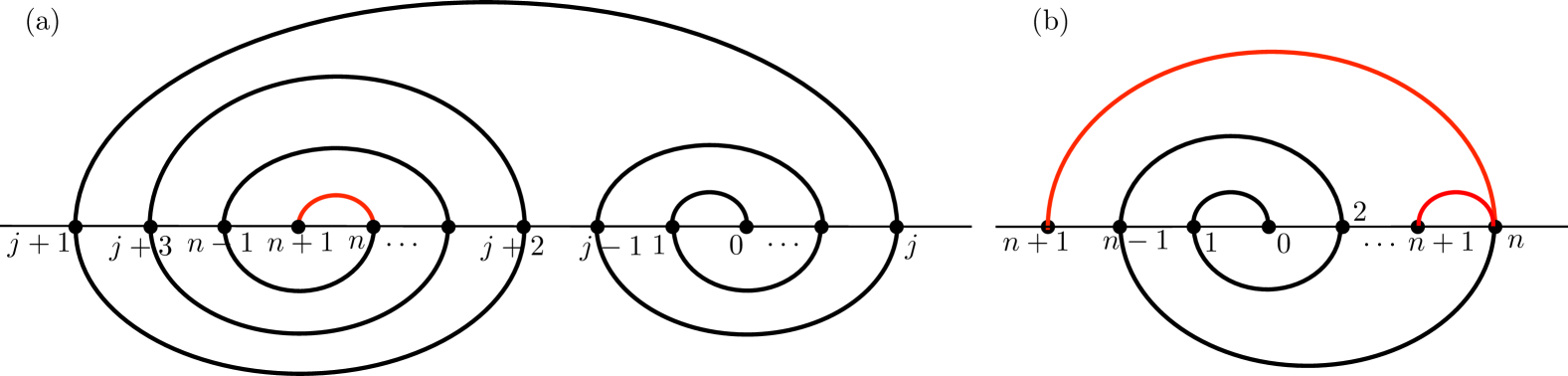
Figure 2. (a) Addition of a single face in Case 1 and (b) Case 2 of Theorem 2.5.

Case 2: The $n$-th face is on the outside of the folded strip in the existing layer ordering for $M^{n-1}$. As seen in Figure 2(b), this case allows for two places to put stamp $(n+1)$, namely $I(n-2,n)$ or $I(\pm\infty,n-1)$, with exactly one of the ways keeping the last face on the outside.

Thus we have that $c(M^{n})=c(M^{n-1})+1$. Solving this recurrence with the initial condition $c(M^{1})=1$ gives us $c(M^{n})=n$. ∎

3. Specific Mountain-Valley Assignments

3.1. The $M^{a}V^{b}$ Assignment

Let’s count the number of valid layer orderings in MV assignments with only two blocks. Removing symmetries, it suffices to consider MV assignments of the form $M^{a}V^{b}$ with $a\geq b$ by Remark 2.4.

Theorem 3.1.

The MV assignment $M^{a}V^{b}$ on the $1\times(a+b+1)$ strip, where $a>b+1,b>4$ folds in $ab+b^{2}-b+1$ ways.

Proof.

Beginning with one of the $a$ valid stamp foldings for $M^{a}$, we will calculate the number of ways to fold the second block, $V^{b}$. Let the extreme left and right faces of this folding of $M^{a}$ be $j$ and $j+1$, for some $j\in{0,\dots,a-1}$.

If $j+1=a$ then the folding of $M^{a}$ is a single spiral starting with face 0 in the center, as seen in Figure 3(a). In this case face $a+1$ must be folded in $I(a,\pm\infty)$ and we have choices for the remaining $b-1$ faces. Face $a+2$ can go into $I(a,a+1)$, in which case it must deterministically spiral inwards from there. In fact, this option of deterministically spiraling inwards is always an option at every decision point in folding $V_{b}$. The other options are to spiral outwards, shown in red in Figure 3(a) (i.e., fold into $I(a-1,\pm\infty)$, then into $I(a+1,\pm\infty)$, and so on), or to spiral into the $M^{a}$ spiral by folding into $I(a-1,\pm\infty)$, then into $I(a-2,a)$ and following the blue path in Figure 3(a). Including the options of spiraling deterministically at every juncture, there are $b$ options in the outward-spiraling red paths and $b-2$ for the inward-spiraling blue paths. Thus the $j+1=a$ case has $2b-2$ ways to fold.

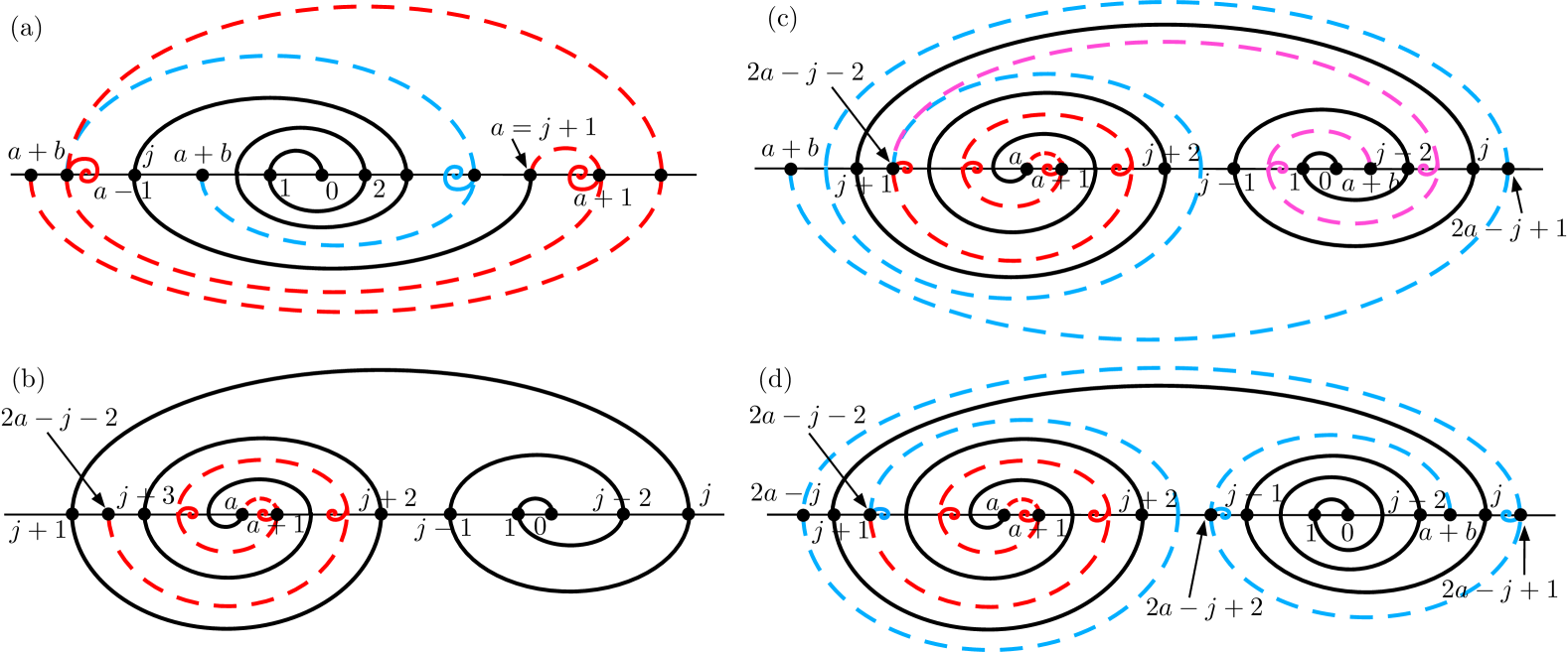
Figure 3. The various cases of Theorem 3.1.

If $j+1<a$ then, given that $a>b+1>4$, the general situation will look something like that shown in Figure 3(b), where the $V^{b}$ folding spirals away from stamp $a$ (shown in red) and assuming it does not deterministically spiral inwards at some point, will reach stamp $2a-j-2$. From there, our folding of $V^{b}$ has three choices:

(1) spiral deterministically at that point, (the small red spiral at stamp $2a-j-2$ in Figure 3(c)),

(2) enter $I(j-2,j)$ (or $I(j-1,j)$ if $j=1$), shown in pink in Figure 3(c), or

(3) enter $I(j-1,j+2)$ (or $I(j,j+2)$ if $j=0$), shown as blue paths in Figure 3(c) and (d).

The only options that do not depend on $j$ are (1) and (3) when the folding of $V^{b}$ spirals away outside the folding of $M^{a}$. We consider these together, with the red path (and its deterministic spiral options at each juncture) in Figure 3(b) and the blue path in Figure 3(c). This has $b$ ways to fold, as there are $b-1$ places to spiral inwards (including the option (1) case) plus the one case where the whole path spirals outward. Any of these $b$ ways to fold $V^{b}$ can happen with any of the $a$ ways to fold $M^{a}$ except for the $j+1=a$ case described earlier. Thus there are $(a-1)b=ab-b$ ways to fold this case.

Option (2) assumes we have not previously spiraled deterministically at a previous juncture and only happens if $2a-j-1\leq a+b$ (otherwise the red path in Figure 3(b) never leaves the spiral centered at stamp $a$). That is, $a-b-1\leq j$. If $j=a-b-1$ then we have only one way to fold the one remaining stamp of $V^{b}$. With each increase in $j$ we have one more stamp of $V^{b}$ to fold along the pink path of Figure 3(c), with the extreme case being $j=a-2$ and all $b$ stamps of $V^{b}$ folding along the pink path, which has $b$ ways to fold. Thus in this case, ranging over all possible values of $j$, we have $1+2+\dots+b=b(b+1)/2$ ways to fold in this case.

The remaining case is option (3) where our folding enters $I(j-1,j+2)$, loops around the $M^{a}$ folding, and then stamp $2a-j+2$ re-enters at $I(j-1,2a-j-1)$, as shown in the blue path in Figure 3(d). For this to occur, we need $2a-j+2\leq a+b$, or $a-b+2\leq j$. Note that $j$ is at most $a-2$, so for this case to exist, $b$ must be at least 4. This is essentially the same as the previous case, except we make three folds before entering $I(j-1,2a-j-1)$. Thus there are $1+2+\dots+(b-3)=(b-2)(b-3)/2$ ways to fold this case.

Putting all these cases together, for $a-b>1$ and $b\geq 4$, there are

$$(2b-2)+(ab-b)+\frac{b(b+1)}{2}+\frac{(b-2)(b-3)}{2}=ab+b^{2}-b+1$$

ways to fold the MV assignment $M^{a}V^{b}$. ∎

3.1.1. Edge Cases

There are also the edge cases that need to be considered. First, if $b<4$, the last case in the above proof cannot occur, and thus the $\frac{(b-2)(b-3)}{2}$ must be removed from the sum. Note that this only affects the sum when $b<2$, as $\frac{(b-2)(b-3)}{2}$ equals zero when $b$ is either $2$ or $3$.

Also, if $a-b$ is zero or one, the folding path can reach the center of the second spiral, which limits the number of elements of the option (2). So, in option (2) where $a-b=1$, we only have $1+2+\dots+b-1=b(b-1)/2$ paths, and $M^{a}V^{a+1}$ folds in $2a^{2}-a+1$ ways.

In the case where $a=b$, we have two fewer steps until reaching the center of the spiral, and thus option (2) has $1+2+\dots+b-2$ elements, making $M^{a}V^{a}$ fold in $2a^{2}-3a+2$ ways.

3.2. The 2-alternating Assignments

We have seen a class of MV assignments that fold in a number of ways polynomial in the length of the string. In this section we consider the class of assignments with blocks of size two. The first few examples are $MM$, $MMVV$, $MMVVMM$, and so on. We refer to these assignments as 2-alternating. Formally, the 2-alternating assignment with $m$ blocks is $(M^{2}V^{2})^{m/2}$ for even $m$ and $(M^{2}V^{2})^{(m-1)/2}M^{2}$ for odd $m$. We now aim to count precisely the number of ways this pattern folds.

Theorem 3.2.

The 2-alternating assignment on the $1\times(2m+1)$ strip with $m$ blocks folds in $\displaystyle C_{\lfloor\frac{m}{2}\rfloor+1}C_{\lceil\frac{m}{2}\rceil+1}$ ways, where $C_{i}$ is the $i$-th Catalan number.

The proof has two main parts. First, we show that counting the valid layer orderings for these MV assignments is equivalent to counting restricted walks in ${\mathbb{Z}}^{2}$ in Lemma 3.5. We then show that the number of such walks is the product of Catalan numbers as specified in the Theorem.

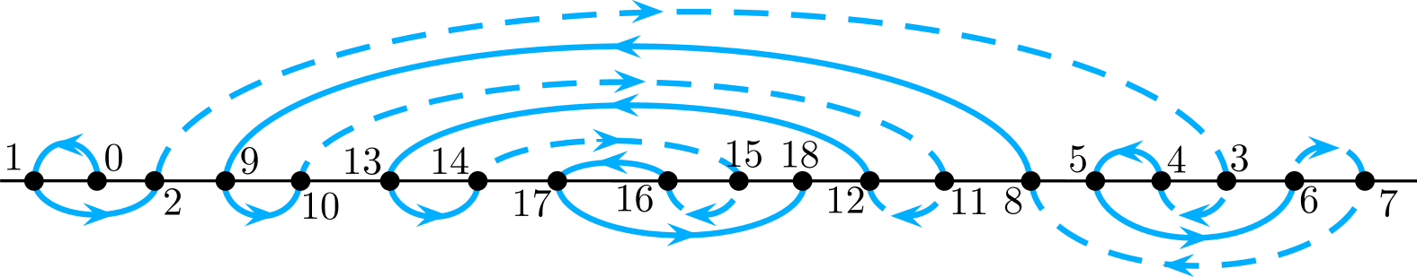
Figure 4. An example of a 2-alternating assignment folding of $(M^{2}V^{2})^{4}M^{2}$.

To build up to this, we make some observations about the inherent structure of 2-alternating assignments; an example is shown in Figure 4. Observe that when viewing our foldings as meanders, arcs $(i,i+1)$ lie above the horizontal line for even $i$, and below for odd $i$; we refer to these as top arcs and bottom arcs respectively. Note that our convention is that the first face $0$ faces right and the first $M$ crease $(0,1)$ is a top arc, which means in the meander drawing this arc will be drawn from right-to-left; i.e., $\sigma(1)<\sigma(0)$. Perpetuating this, we have that each initial $M$ in an $M^{2}$ will be a top arc traveling right-to-left in the meander drawing, while the second $M$ will be a bottom arc going left-to-right. The $V^{2}$ instances will be similar but with the directions reversed.

We call a bottom arc $(i,i+1)$ uncovered if $I(i,i+1)$ is not contained in any $I(j,j+1)$ for bottom arc $(j,j+1)$, with $j<i$. Otherwise, we call $(i,i+1)$ covered. These special arcs will be key to counting the valid layer orderings.

Lemma 3.3.

In every possible layer ordering satisfying a 2-alternating assignment, the two following conditions are satisfied:

1. Suppose $(i,i+1)$ is a top arc in a 2-alternating assignment. Then given a layer ordering of faces 0 through $i$, face $i+1$ has precisely one place to be inserted in the permutation.

2. The uncovered bottom arcs are arranged such that all of the mountain arcs are to the left of all the valley arcs. That is, if $(i,i+1)$ is an uncovered bottom mountain arc and $(j,j+1)$ is an uncovered bottom valley arc, then $\sigma(i)<\sigma(j)$. Further, if the assignment ends with a $V$, the position of the final face must be the endpoint of the leftmost uncovered bottom valley arc. Otherwise, the position of the final face must be the endpoint of the rightmost uncovered bottom mountain arc.

Proof.

We prove this by induction on the number of stamps in a 2-alternating assignment. It is trivially true for the first bottom mountain arc. Now suppose the Lemma is true for 2-alternating assignments on $i$ stamps. Given a valid folding of a 2-alternating assignment on $i+1$ stamps, drawn as a meander, we have that our meander picture satisfies the Lemma for points $0$ up to $i$ with $(i-1,i)$ being the endpoint of a bottom arc, which we for the moment assume is a mountain arc. See Figure 5 for an illustration of this.

Let $k$ be the left-most face in our drawing that is part of the left-most bottom valley arc. Then by the induction hypothesis we have $\sigma(i)<\sigma(k)$. Next, we will show that $\sigma(i+1)<\sigma(k)$ and thus there is only one place for face $i+1$ to be folded: $I(i,k)$ (which will prove part (1) of the Lemma by induction). Suppose for the sake of contradiction that $\sigma(k)<\sigma(i+1)$. Since $(k-1,k)$ is a valley by our inductive hypothesis, the arc $(k,k+1)$ must be a top $M$ arc with $\sigma(k+1)<\sigma(k)$. We also know that $\sigma(k+1)<\sigma(i)$. If not, $(k+1,k+2)$ would be a bottom mountain arc contained in $I(i,k)$ violating the assumption of the inductive hypothesis that $(i-1,i)$ is the rightmost mountain arc. But then $\sigma(k+1)<\sigma(i)<\sigma(k)<\sigma(i+1)$, so $(i,i+1)$ and $(k,k+1)$ intersect and the layer ordering is not valid.

Then $(i+1,i+2)$ will be a bottom $M$ arc in the left direction that folds face $i+2$ into an interval to the left of $I(j,k)$, which maintains property (2) of the Lemma. The case where $i$ was the endpoint of a valley arc is symmetric and the same reasoning applies. ∎

Figure 5. Illustration of the proof of Lemma 3.3. Not all arcs are shown.

It is important to note that this structure would not be present if the MV assignment was different. For general assignments, the uncovered arcs could be intermixed between mountain and valley, and it is rare that the structure would require that any face has only one place to fold.

This means that to count the total ways to build the folding, we need only pay attention to the bottom arcs and where they go. The utility of Lemma 3.3 is that we need only maintain the number of uncovered bottom arcs of both kinds. Consider an example illustrated in Figure 6: Say we have already folded the faces up to $i$ and there are three uncovered bottom mountain arcs and two valley arcs. Then face $i+1$ with a bottom arc $(i,i+1)$, must fold in the gaps (uncovered intervals) between these arcs or the gap to the far left or right. If we know that $(i,i+1)$ is a valley, there are four options including entering the left-most, unbounded gap before the rightmost mountain, and otherwise there are three options for if $(i,i+1)$ is a mountain.

Figure 6. With only uncovered bottom arcs shown, at $i$ there are $4$ potential gaps to the left and $3$ to the right. If $(i,i+1)$ is a mountain arc then $f(i)=4$ and $b(i)=3$. Otherwise $f(i)=3$ and $b(i)=4$. Solid arcs correspond to mountains, while dashed arcs are valleys.

To capture this idea, define $f(i)$ to be the number of potential gaps for $(i,i+1)$ to enter in the “forward” direction; if $(i,i+1)$ is a valley arc then these are the gaps to left of $i$, otherwise they are those to the right. Then define $b(i)$ to be the gaps “behind” $i$. Notice that between consecutive bottom arcs, the direction of forwards and backwards switches. We then have the following.

Lemma 3.4.

Let $i$ be the starting point of a bottom arc with values $f(i)$ and $b(i)$. Then, $f(i+2)=b(i)+1$ and $b(i+2)\in\{1,\dots f(i)\}$, where $b(i+2)$ depends on where face $i+1$ is folded.

Proof.

Suppose face $i+1$ is placed between $j$ and $k$. Then for $i+2$, the gaps in the direction of the arc will be those gaps that were behind $(i,i+1)$ including the newly created gap $I(i+1,k)$. Conversely, because $i+1$ can be folded into any of the $f(i)$ gaps and it will create a new one in front of it, this will give some number of gaps behind $(i+2,i+3)$ that is at minimum 1 and at most $f(i)$. ∎

We can now completely abstract the process of counting valid layer orderings to the following.

Lemma 3.5.

Let $\mu$ be the 2-alternating assignment on a $1\times(2m+1)$ strip. Then $c(\mu)$ is given by the number of walks of length $m$ in ${\mathbb{Z}}^{2}$ starting at $(2,1)$ with the allowed steps of the form $(a,b)\to(b+1,i)$ where $i\in\{1,\dots,a\}$.

Proof.

Starting with $i=1$, we let $f(i)=f(1)=2$ and $b(i)=b(1)=2$ and imagine a walk in ${\mathbb{Z}}^{2}$ as described starting at $(2,1)$. At each step in our walk we add 2 to the index $i$ and let $(f(i+2),b(i+2))$ be point in ${\mathbb{Z}}^{2}$ in our walk. Thus our walk can bring us to any of the positions described in Lemma 3.4, and any of these walks in ${\mathbb{Z}}^{2}$ can determine an $M^{2}$ or a $V^{2}$ part of our 2-alternating stamp folding. We take $m$ steps to reach index $2m+1$, the final index in the permutation which we know to be of length $2m+1$. ∎

To count the number of ways to perform this walk, we introduce a matrix that will encode the state information at each step.

Definition 3.6.

Let $i,j\in\mathbb{N}$. We define a matrix $X(m)$ such that $X(m)_{i-1,j}$ is the number of walks of length $m$ in $\mathbb{Z}^{2}$ starting at $(2,1)$ with steps as defined above that end at $(i,j)$. We omit rows and columns of all zeroes. See below for an example when $m=4$.

$$X(4)=\blockarray{ccccll}&&j\\ &\textbf{1}&\textbf{2}&\textbf{3}&&\\ \block{[cccc]ll}&4&4&2&&\textbf{2}\\ &4&4&2&&\textbf{3}&i\\ &2&2&1&&\textbf{4}\\$$

One key feature we want to know about $X(m)$ is its dimensions. This will be important later as we construct a matrix representation of taking a single step that will rely on the dimensions of $X(m)$.

Lemma 3.7.

Let $(a,b)$ be the position in a walk after $m$ steps. Then $2\leq a\leq\lfloor\frac{m+4}{2}\rfloor$ and $1\leq b\leq\lceil\frac{m+2}{2}\rceil$.

Proof.

We proceed by induction on $m$. Consider $(a,b)$ a position in the walk after $m+1$ steps. Then by definition, $b\geq 1$. Also by definition, there is an element $(c,d)$ in the walk after $m$ steps such that $a=d+1$ and $b\leq c$. By the inductive hypothesis, $d\geq 1$. So $a\geq 2$. Also by the inductive hypothesis, $c\leq\lfloor\frac{m+4}{2}\rfloor\text{ and }d\leq\lceil\frac{m+2}{2}\rceil$. Thus $b\leq\lfloor\frac{m+4}{2}\rfloor=\lceil\frac{(m+1)+2}{2}\rceil\text{ and }a\leq\lceil\frac{m+4}{2}\rceil=\lfloor\frac{(m+1)+4}{2}\rfloor$. ∎

Now, because of Lemma 3.7, we can see that $X(m)$ must always have dimension $\lfloor\frac{m+2}{2}\rfloor\times\lceil\frac{m+2}{2}\rceil$. We say that accessing any index outside of these bounds will return a value of 0. We can now define the matrix representation of taking a single step in a walk on ${\mathbb{Z}}^{2}$ mentioned above.

Definition 3.8.

Define the matrix $A(m)$ to be the $(\lfloor\frac{m+2}{2}\rfloor+1)\times\lfloor\frac{m+2}{2}\rfloor$ matrix

$$\begin{bmatrix}1&1&...&1&1\\ 1&1&...&1&1\\ 0&1&...&1&1\\ &&...&&\\ 0&0&...&1&1\\ 0&0&...&0&1\end{bmatrix}$$

That is, $A(m)$ is an upper triangular matrix of all ones with a row of ones appended to the top.

Now we prove that the definition of $A(m)$ given above is actually helpful in taking a step.

Lemma 3.9.

Applying $A(m)$ to $X(m)$ and then transposing the result is the same as taking a step from the positions represented by $X(m)$. In other words,

$$X(m+1)=(A(m)X(m))^{T}$$

Proof.

When taking a step at position $(c,d)$, for each positive integer $i$ less than or equal to $c$, we can move to position $(d+1,i)$. Let $(a,b)$ be a position in the walk that can be reached after $m+1$ steps. The number of ways to reach $(a,b)$ in $m+1$ steps is thus equal to the sum of the number of ways to reach each element $(i,a-1)$ in $m$ steps, where $i\geq b$. Since $X(m+1)_{a-1,b}$ is the number of ways to reach position $(a,b)$ in $m+1$ steps,

$$X(m+1)_{a-1,b}=\sum_{i=b-1}^{\lfloor\frac{m+2}{2}\rfloor}X(m)_{i,a-1}$$

This operation is the same as applying $A(m)$ to $X(m)$ and then transposing the result. ∎

Now that we have a matrix for both taking a single step and representing all valid positions after taking $m$ steps, we can use matrix multiplication to easily compute the entries in $X(m)$ for any $m$.

Definition 3.10.

Catalan’s Triangle is a triangle of numbers such that each entry is equal to the sum of the entries of the previous row that are not to the right of the current position. One important property of Catalan’s triangle is that the elements in the $n^{th}$ row sum to the $n^{th}$ Catalan number. The first five rows of Catalan’s triangle are shown in Figure 7(b). For more on this triangle, see [1].

$\begin{bmatrix}25&25&15&5\\ 25&25&15&5\\ 15&15&9&3\\ 5&5&3&1\end{bmatrix}$

(a) $X(6)$

Row
1	1 1
2	1 2 2
3	1 3 5 5
4	1 4 9 14 14
5	1 5 14 28 42 42

(b) The first 6 rows of Catalan’s triangle.

Figure 7. The third row of Catalan’s Triangle flipped backwards is equal to the last row and column of $X(6)$.

It turns out we can connect the entries of our matrices $X(m)$ to this triangle. (See Figure 7(a) and Figure 7(b) for an example.)

Lemma 3.11.

The last column of $X(m)$ is equal to the $\lfloor\frac{m}{2}\rfloor^{th}$ row of Catalan’s triangle and the last row of $X(m)$ is equal to the $\lceil\frac{m}{2}\rceil^{th}$ row of Catalan’s triangle.

Proof.

We proceed by induction on $m$. $X(2)$ is the $2\times 2$ matrix of all ones, whose last row and column equals the first row of Catalan’s triangle.

By Lemma 3.9, $X(m+1)=(A(m)X(m))^{T}$. We will first prove the claim holds for the last column. Let $i\in\mathbb{N}$ such that $1\leq i\leq\lfloor\frac{(m+1)+2}{2}\rfloor$. By matrix multiplication,

$$X(m+1)_{i,\lceil\frac{(m+1)+2}{2}\rceil}=\sum_{j=\lceil\frac{m+1}{2}\rceil}^{\lfloor\frac{m+2}{2}\rfloor}X(m)_{j,i}=X(m)_{\lfloor\frac{m+2}{2}\rfloor,i}$$

So the last column of $X(m+1)$ is equal to the last row of $X(m)$, which is the $\lceil\frac{m}{2}\rceil^{th}=\lfloor\frac{m+1}{2}\rfloor^{th}$ column of Catalan’s triangle by the inductive hypothesis.

Now we prove the claim holds for the last row. Let $i\in\mathbb{N}$ such that $1\leq i\leq\lceil\frac{(m+1)+2}{2}\rceil$. By matrix multiplication,

$$X(m+1)_{\lfloor\frac{(m+1)+2}{2}\rfloor,i}=\sum_{j=i-1}^{\lceil\frac{m+2}{2}\rceil}X(m)_{\lfloor\frac{m+2}{2}\rfloor,j}$$

So the last column of $X(m+1)$ is dependent only on the last row of $X(m)$, which by our inductive hypothesis is equal to the $\lceil\frac{m}{2}\rceil^{th}$ row of Catalan’s triangle, and this recurrence is identical to the one that generates the Catalan triangle. ∎

We now know the last row and column of any $X(m)$, but we still need to know the other entries. Interestingly, each element of the matrix is equal to the product of the element in its same row and last column and the element in its same column but last row. This will be defined rigorously in the following lemma.

Lemma 3.12.

Let $i,j\in\mathbb{N}$ such that $1\leq i\leq\lfloor\frac{m}{2}\rfloor$ and $1\leq j\leq\lceil\frac{m}{2}\rceil$. Then

$$X(m)_{i,j}=X(m)_{i,\lceil\frac{m+2}{2}\rceil}\cdot X(m)_{\lfloor\frac{m+2}{2}\rfloor,j}$$

Proof.

We proceed by induction on $m$. By Lemma 3.9, $X(m+1)=(A(m)X(m))^{T}$. $A(m)$ has dimension $(\lfloor\frac{m+2}{2}\rfloor+1)\times\lfloor\frac{m+2}{2}\rfloor$ by Definition 3.8. Let $i,j$ be natural numbers such that $1\leq i\leq\lfloor\frac{m+1}{2}\rfloor$ and $1\leq j\leq\lceil\frac{m+1}{2}\rceil$. Using matrix multiplication, we see that

$$X(m+1)_{i,j} =\sum^{\lfloor\frac{m+1}{2}\rfloor}_{k=i-1}\sum^{\lceil\frac{m+1}{2}\rceil}_{\ell=j-1}X(m)_{k,\ell}$$

(Inductive Hypothesis) $$=\sum^{\lfloor\frac{m+1}{2}\rfloor}_{k=i-1}X(m)_{k,\lceil\frac{m+1}{2}\rceil}\sum^{\lceil\frac{m+1}{2}\rceil}_{\ell=j-1}X(m)_{\lfloor\frac{m+1}{2}\rfloor,\ell}$$

By the Catalan’s triangle recurrence and Lemma 3.11, this is equal to $X(m+1)_{i,\lceil\frac{(m+1)+2}{2}\rceil}\cdot X(m+1)_{\lfloor\frac{(m+1)+2}{2}\rfloor,j}$. ∎

Proof of Theorem 3.2.

The number of walks of length $m$ in $\mathbb{Z}^{2}$ satisfying the above conditions is equal to the sum of the elements in $X(m)$ since $X(m)$ contains the multiplicity of each reachable position after $m$ steps. By Lemma 3.12, the sum of the elements in $X(m)$ is equal to the sum of the elements in its last column multiplied with the sum of the elements in its last row. By Lemma 3.11, these elements are exactly the elements in the $\lfloor\frac{m}{2}\rfloor^{th}$ and $\lceil\frac{m}{2}\rceil^{th}$ rows of Catalan’s triangle, respectively. So the sum of the elements in $X(m)$ is equal to the sum of the elements in the $\lfloor\frac{m}{2}\rfloor^{th}$ row of Catalan’s triangle multiplied by the elements in the $\lceil\frac{m}{2}\rceil^{th}$ row, which are known to be the $\lfloor\frac{m}{2}\rfloor+1^{th}$ and $\lceil\frac{m}{2}\rceil+1^{th}$ Catalan numbers, respectively. ∎

4. Bounds on the Folding Number of General Mountain-Valley Assignments

We have previously computed the number of valid layer orderings for specific patterns of mountain-valley assignments. Now, we will look at the problem for general assignments and compute both lower and upper bounds on the number of valid layer orderings. Each bound occurs from analyzing the number of ways to add an additional block to an existing valid layer ordering.

4.1. Lower Bound

We begin by computing the lower bound. For convenience, let ${\llbracket}a_{1},a_{2},\dots,a_{m}{\rrbracket}$ refer to the MV assignment $M^{a_{1}}V^{a_{2}}\dots(M/V)^{a_{m}}$.

Lemma 4.1.

For an arbitrary mountain-valley assignment ${\llbracket}a_{1},a_{2},\dots,a_{m}{\rrbracket}$,

$$c({\llbracket}a_{1},a_{2},\dots,a_{m-1}{\rrbracket})\cdot\min(a_{m-1}+1,a_{m})\leq c({\llbracket}a_{1},a_{2},\dots,a_{m}{\rrbracket})$$

Proof.

Consider an arbitrary folding of the first $m-1$ blocks viewed as a meander drawing. We will show that there are always at least $\min(a_{m-1}+1,a_{m})$ different ways to draw the $m$th block. Intuitively, these $\min(a_{m-1}+1,a_{m})$ ways come from the paths that remain directly adjacent to the previous block, retracing the spiral.

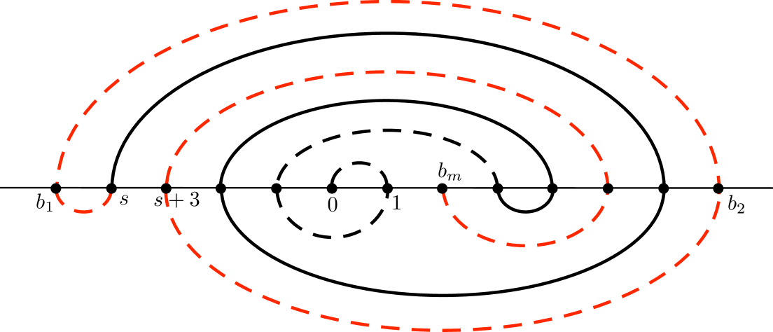
Figure 8. Meander representing $V^{3}M^{4}V^{5}$. The black represents the previous meander for $V^{3}M^{4}$ and the red represents the constructed path for the final block.

Let $s=\sum_{i=1}^{m-1}a_{i}$ be the number of creases in the first $m-1$ blocks.

Let us now construct a valid path for the $m$th block after the first $m-1$ blocks have been folded; an example is shown in red in Figure 8. Let $b_{i}$ be the $i$th face of the $m$th block, so $b_{i}=s+i$. Place $b_{1}$ in the first possible gap, directly adjacent to face $s$. Then, place $b_{2}$ in the first gap adjacent to face $s-1$, such that crease $(b_{1},b_{2})$ travels around creases $(s,s-1)$ with no portion of the meander between the two creases. This process continues, placing each $b_{i}$ in the gap adjacent to face $s-i+1$ until there are no remaining faces in one of the last two spirals, i.e. $i>\min(a_{m-1}+1,a_{m})$.

Claim: This process must yield a valid, non-intersecting path.

Assume for the sake of contradiction that the path outlined above intersects a previous arc. Let the first intersection occur when drawing crease $(b_{i},b_{i+1})$. Assume this crease intersects some crease $(k,k+1)$. This implies, by the crossing condition, that exactly one of $k,k+1$ lies in $I(b_{i},b_{i+1})$. Additionally, by construction there are no faces from the first $m-1$ blocks in either of the intervals $I(b_{i},s-i+1),I(b_{i+1},s-i)$. So, exactly one of $k,k+1$ must lie in $I(s-i+1,s-i)$. However, we know from Definition 2.1(2) that either zero or two of $k,k+1$ lie in $I(s-i+1,s-i)$, creating a contradiction.

Now, we can generate the remaining paths. For each $b_{i}$, instead of following along the path outlined above, the path can instead enter the gap $I(b_{i},s-i+1)$ and spiral inwards. So, we get an additional path for each $b_{i}$, giving the total of $\min(a_{m-1}+1,a_{m})$ paths. ∎

Theorem 4.2.

For an arbitrary mountain-valley assignment ${\llbracket}a_{1},a_{2},\dots,a_{m}{\rrbracket}$,

$$c({\llbracket}a_{1},a_{2},\dots,a_{m}{\rrbracket})\geq a_{1}\cdot\prod_{i=2}^{m}\min(a_{i-1}+1,a_{i})$$

Proof.

From Theorem 2.5, we know there are exactly $a_{1}$ ways to fold the first block. Then, we can repeatedly apply Lemma 4.1 to get this overall bound. ∎

4.2. Upper Bound

Next, we move onto consideration of an upper bound.

Lemma 4.3.

For an arbitrary mountain-valley assignment ${\llbracket}a_{1},a_{2},\dots,a_{m}{\rrbracket}$,

$$c({\llbracket}a_{1},a_{2},\dots,a_{m}{\rrbracket})\leq c({\llbracket}a_{1},a_{2},\dots,a_{m-1}{\rrbracket})\left[a_{m}+\sum_{i=1}^{m-1}2a_{i}\right]$$

Proof.

To begin, consider any valid meander $\mathcal{M}$ corresponding to the first $m-1$ blocks of the MV assignment. We wish to show that there are at most $a_{m}+2\sum_{i=1}^{m-1}a_{i}$ ways to draw the final block. To do this, we show that for each gap other than the two outside of $\mathcal{M}$ there are at most two possible drawings of the $m$th block path ending in that gap.

Assume for the sake of contradiction that there are three distinct paths, $\phi,\chi,\psi$ for drawing the $m$th block such that their endpoints are all in some gap $I(a,b)$, with $a,b<a_{1}+\dots+a_{m-1}$. For each path, only consider the portion of the path before the path starts spiraling inwards, i.e. when the path enters $I(a,b)$ and never leaves that gap. From Theorem 2.5, we know that once a block begins spiraling inwards into a gap, the rest of the locations of the faces are determined.

Figure 9. Shifting points in the $m$th block in Claim 4.4 in Lemma 4.3.

Claim 4.4.

These paths, up to and including where they enter $I(a,b)$, can always be drawn without intersecting.

Proof of Claim 4.4: Assume paths $p$ and $q$ must intersect. This means that there are arcs $(i,i+1)$ in $p$ and $(j,j+1)$ in $q$ that violate Definition 2.1 (2). Then the end of $\mathcal{M}$ can only be in one of the intervals $I(i,j),I(i+1,j+1)$. Since there are no arcs between either $i,j$ or $i+1,j+1$, we can move one of the points through an empty interval without changing $\mathcal{M}$ (see Figure 9 for an illustration of this), and so we can draw the paths as desired.

These three distinct curves with the same endpoints split ${\mathbb{R}}^{2}$ into at least 3 regions, with 2 bounded regions. Furthermore, we notice that the meander $\mathcal{M}$ corresponding to the first $m-1$ blocks cannot intersect any of these three curves. So, the entirety of the meander must be contained in one of these three regions and there exists a bounded region without any of the faces from the first $m-1$ blocks. Without loss of generality, assume the region bounded by $\psi$ and $\phi$ does not contain $\mathcal{M}$.

Claim 4.5.

The paths $\psi$ and $\phi$ must be equivalent as meanders.

Proof of Claim 4.5: Suppose not. Then assume $\psi$ and $\phi$ are equivalent (i.e., follow the same path through the meander drawing) for the first $\ell$ steps but not for the $(\ell+1)$-st step. That is, the endpoint of the $(\ell+1)$st step in $\psi$ must be in a different location $x$ than the location $y$ of the same endpoint in $\phi$, and there must be an obstruction in the meander drawing that prevents shifting $x$ and $y$ to be the same location. Since $\mathcal{M}$ is not in the region between $\psi$ and $\phi$, the obstruction must be the previous $\ell$ steps of $\psi$, which are the same as those of $\phi$. However, in this case, the two paths $\psi$ and $\phi$ cannot possibly end in the same location, as the path that goes around the previous portion of $\phi/\psi$ cannot reenter the desired interval without intersecting the previous portion of the curve.

Thus, for each interval gap $I(a,b)$ in $\mathcal{M}$, we could, provided that $a_{m}$ is large enough, have the $m$th block path spiral through $\mathcal{M}$ and end in $I(a,b)$. By the above argument, there are at most two such distinct paths that can be drawn. Furthermore, the number of possible interval gaps $I(a,b)$ is bounded by the number of stamps in $\mathcal{M}$, which is $a_{1}+a_{2}+\dots+a_{m-1}$.

We must also consider the possibility that the path for the final block ends in one of the unbounded gaps, either to the left or right of $\mathcal{M}$. By Theorem 2.5, there are $a_{m}$ ways to draw this option. Overall there are at most

$$a_{m}+\sum_{i=1}^{m-1}2a_{i}$$

ways to draw the last block. ∎

Theorem 4.6.

For an arbitrary mountain-valley assignment ${\llbracket}a_{1},a_{2},\dots,a_{m}{\rrbracket}$,

$$c({\llbracket}a_{1},a_{2},\dots,a_{m}{\rrbracket})\leq a_{1}\cdot\prod_{i=2}^{m}\left[a_{i}+\sum_{j=1}^{i-1}2a_{j}\right]$$

Proof.

Much like in the proof of Theorem 4.2, we observe that the first block can fold in $a_{1}$ ways, due to Theorem 2.5, and then apply Lemma 4.3 repeatedly to get this general upper bound. ∎

5. Experimental Results

In searching for patterns and observations on the ways stamps fold, we turned to using software to compute the answer for various classes of assignments. A simple but naive way to compute $c(\mu)$ for an assignment $\mu$ is to consider all $n!$ permutations of the faces and directly apply the definition of a valid layer ordering. This approach is inefficient because even for assignments that fold in many ways, the value of $c(\mu)$ is nowhere near $n!$ and so the running time is exponentially slower than the value of $c(\mu)$.

A faster approach has been developed in [7] for computing the stamp folding numbers without specified MV assignments. The design of their algorithm is recursive and relies on the thinking in Lemma 3.4 that has been used throughout this paper. There, they devise a search tree in which nodes represent partial layer orderings and contain information regarding which gaps are possible to enter next. In particular, in every state $X$ of the algorithm corresponding to a permutation $\sigma_{i}$ of the first $i$ faces, two lists $L_{X}$ and $R_{X}$ are stored containing gaps $(j,k)$ that are to the left and right of $i$ for which placing $i+1$ would not create crossing arcs. The algorithm runs in $O(c(\mu))$ time for an assignment $\mu$.

To adapt their method to count only layer orderings that respect in an inputted MV assignment, in a state $X$, we still store both $L_{X}$ and $R_{X}$, but when iterating to the next state we consider only gaps on the appropriate side of the current face so that the relative order of adjacent faces accord with the MV assignment.

With this, we ran experiments to get towards new results.

5.1. Maximally Foldable Assignment

The original stamp folding problem asks for the number of ways to fold a $1\times n$ stamp flat. To this end, we investigate the maximally foldable MV assignment for each $1\times n$ strip to see if we can find a pattern there. We used our faster algorithm to manually find the maximal assignment for each $n$ up to $21$. Let the first crease be a valley and exclude MV assignments that are the same up to the symmetries described in Remark 2.4. Then the MV assignments shown in Table 1 are maximally foldable. Different MV assignments are separated by semicolons.

$\mathbf{n}$	Best Assignment
2	$V$
3	$V^{2}$
4	$V^{3}$
5	$V^{4};V^{3}M;V^{2}M^{2}$
6	$V^{3}M^{2};V^{2}MV^{2}$
7	$V^{4}M;V^{3}MV^{2};V^{3}M^{3}$

$\mathbf{n}$	Best Assignment
8	${\llbracket}3,2,2{\rrbracket}$
9	${\llbracket}3,2,3{\rrbracket}$
10	${\llbracket}3,2,2,2{\rrbracket}$
11	${\llbracket}3,2,2,1,2{\rrbracket}$
12	${\llbracket}2,2,3,2,2{\rrbracket}$
13	${\llbracket}3,2,3,2,2{\rrbracket}$
14	${\llbracket}3,2,3,2,3{\rrbracket}$

$\mathbf{n}$	Best Assignment
15	${\llbracket}2,2,3,2,2,1,2{\rrbracket}$
16	${\llbracket}2,2,3,2,2,2,2{\rrbracket}$
17	${\llbracket}2,2,3,2,3,2,2{\rrbracket}$
18	${\llbracket}2,1,2,2,3,2,2,1,2{\rrbracket}$
19	${\llbracket}2,2,3,2,3,2,2,1,2{\rrbracket}$
20	${\llbracket}2,2,3,2,3,2,2,1,2{\rrbracket}$
21	${\llbracket}2,2,3,2,2,2,3,2,2{\rrbracket}$

Table 1. Maximally foldable MV Assignments

While we have been unable to find a closed form for the exact maximally folding assignment, we have noticed the following pattern in the data.

Conjecture 5.1.

For $n\geq 8$, the MV assignment that folds in the most ways consists only of blocks of size 1, 2, and 3. Furthermore, there are no two consecutive blocks of size 3.

Assuming the above conjecture is correct, we can find the maximally folding assignment and the number of ways it folds for larger $n$. By only considering assignments that satisfy the conditions, we have been able to plot $n$ vs the number of ways the maximally foldable assignment folds for up to $n=33$ and found it to be roughly linear on a logarithmic scale and seems to closely fit $2^{n}/n^{5/4}$, as shown in Figure 10.

Figure 10. Number of ways the maximally foldable assignment folds on the $1\times n$ strip of stamps. The curve $2^{n}/n^{5/4}$ is overlayed.

5.2. Assignments with Larger Blocks

We have seen that given an assignment with $m$ blocks the number of ways to fold is polynomial in the block sizes. What if all $a_{i}$ have the same value $k$? Let $S(m,k)$ be the assignment with $m$ blocks of $k$ consecutive creases the same. For example, $S(3,2)=MMVVMM$. Define $p_{m}(k)=c(S(m,k))$.

If we fix $m$ and compute the value of $p_{m}(k)$ starting with $k=2$, we experimentally find that the counts are given by a polynomial of degree $m$, where the leading coefficient is always $\frac{m^{m}}{m!}$. See Table 2 for the computed polynomials.

$m$	$p_{m}(k)=c(S(m,k))$ (interpolated)	Max $k$ verified
$2$	$2k^{2}-3k+2$	All
$3$	$\frac{9}{2}k^{3}-\frac{25}{2}k^{2}+15k-6$	78
$4$	$\frac{32}{3}k^{4}-42k^{3}+\frac{211}{3}k^{2}-53k+15$	33
$5$	$\frac{625}{24}k^{5}-\frac{523}{4}k^{4}+\frac{2289}{8}k^{3}-\frac{1279}{4}k^{2}+\frac{538}{3}k-40$	18
$6$	$\frac{324}{5}k^{6}-392k^{5}+\frac{6275}{6}k^{4}-\frac{9071}{6}k^{3}+\frac{18448}{15}k^{2}-\frac{1589}{3}k+94$	10
$7$	$\frac{117649}{720}k^{7}-\frac{91979}{80}k^{6}+\frac{2611459}{720}k^{5}-\frac{310267}{48}k^{4}+\frac{1249699}{180}k^{3}-\frac{66988}{15}k^{2}+\frac{15873}{10}k-240$	9
$8$	$\frac{131072}{315}k^{8}-\frac{9974}{3}k^{7}+\frac{2164969}{180}k^{6}-\frac{1512017}{60}k^{5}+\frac{5958661}{180}k^{4}-\frac{111029}{4}k^{3}+\frac{9108301}{630}k^{2}-\frac{21339}{5}k+546$	8

Table 2. Experimental results for the number of ways to fold MV assignments with equal block sizes. The polynomials agree with the computed values for each sequence up to the value in the rightmost column.

Approximating each polynomial by its leading term and applying Sterling’s approximation, we get the following conjecture.

Conjecture 5.2.

For any fixed $m$ and sufficiently large $k$,

$$p_{m}(k)\sim\frac{e^{m}k^{m}}{\sqrt{2\pi m}}.$$

5.3. Assignments with More Blocks

It is also interesting to explore the asymptotics of $p_{m}(k)$ for fixed values of $k$ and varied $m$.

Conjecture 5.3.

For fixed $k$, there exists values $\alpha$, $\beta$, and $C$ for which $p_{m}(k)\sim\displaystyle C\frac{\alpha^{m}}{m^{\beta}}$ as $m\to\infty$.

Table 3 contains the best-fit curves of this form to data generated for $k$ up to 7. It is useful to consider $\alpha^{\prime}=\alpha^{1/k}$ as this gives the growth rate in terms of $n$, the length of the strip, as opposed to in $m$, the number of blocks.

$k$	$C$	$\alpha$	$\beta$	$\alpha^{\prime}$
3	0.5216	6.0438	0.8495	1.8215
4	0.4757	8.5899	0.7060	1.7120
5	0.4520	11.1768	0.6321	1.6206
6	0.4372	13.8070	0.5900	1.5489
7	0.2688	16.5082	0.3703	1.4926

Table 3. The $C$, $\alpha$, $\beta$ that fit $p_{m}(k)$ as a function of $m$, with the root-mean-square errors.

The decreasing values of $\alpha^{\prime}$ with increased $k$ suggests that smaller blocks give rise to larger number of ways to fold, supporting 5.1. For reference, when $k=2$, from the proof in Section 3.2, we have $\alpha=4$ and $\alpha^{\prime}=2$.

5.4. Distribution

Finally, we are interested in the distribution of the number of MV assignments that can actually achieve each number of ways to fold flat. We’ve generated some diagrams outlining this relationship in Figure 11.

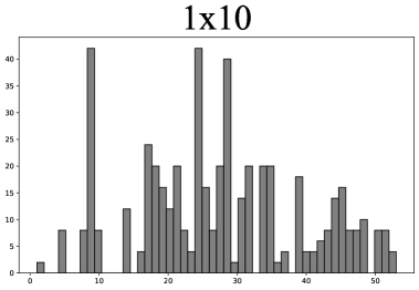
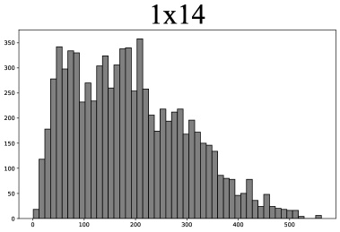
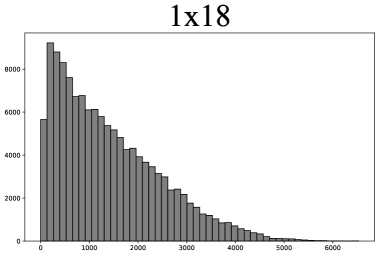
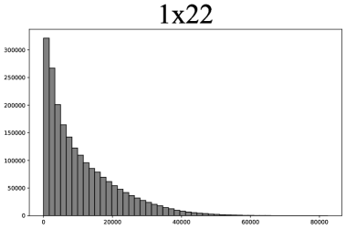
Figure 11. Number of MV assignments vs. Number of ways a given MV assignment can fold flat.

6. Conclusion

We have given a closed form for the number of ways to fold two specific MV assignments, and we have provided bounds for the number of ways any specified MV assignment can fold on the $1\times n$ strip of stamps. To this end, we’ve adapted an existing algorithm that looks at stamp folding as a special class of meanders to generate the number of valid ways a given MV assignment can fold flat. However, there still remains much to be explored in this new perspective on the stamp folding problem.

Open Question 6.1.

Is there a closed form for finding the number of ways a specified MV assignment can fold flat? If not, are there any more general closed forms we can generate for interesting patterns?

Open Question 6.2.

Is it is possible to compute $c(\mu)$ faster than the algorithm described here?

An interesting related area of research involves folding the $2\times n$ grid. This problem is somewhat more complicated as the folding cannot be performed recursively, as is the case in the $1\times n$ strip (see Lemma 2.3). In fact, determining if a specific MV assignment on the $2\times n$ has a valid folding is a challenging problem: [5] gives an $O(n^{9})$ algorithm.

Open Question 6.3.

Can the insights from the $1\times n$ strip of stamps be used in any way to provide insight towards the $2\times n$ case. For each MV assignment on the $1\times n$ strip, is there a corresponding assignment that folds similarly on the $2\times n$ strip?

7. Acknowledgements

This work was supported by NSF grant DMS-2149647. The authors thank Mathematical Staircase, Inc. for funding and supporting the MathILy-EST 2024 REU. The first author was also supported in part by NSF grants DMS-2428771 and DMS-2347000.

References

- [1] D. F. Bailey. Counting arrangements of 1’s and -1’s. Mathematics Magazine, 69(2):128–131, 1996.
- [2] John E. Koehler. Folding a strip of stamps. Journal of Combinatorial Theory, 5(2):135–152, 1968.
- [3] Stéphane Legendre. Foldings and meanders, 2013.
- [4] É. Lucas. Théorie des nombres. Number v. 1 in Théorie des nombres. Gauthier-Villars, 1891.
- [5] Tom Morgan. Map folding by tom morgan, 2012.
- [6] OEIS Foundation Inc. The On-Line Encyclopedia of Integer Sequences, 2024. Published electronically at http://oeis.org.
- [7] Joe Sawada and Roy Li. Stamp foldings, semi-meanders, and open meanders: Fast generation algorithms. The Electronic Journal of Combinatorics [electronic only], 19, 01 2009.
- [8] Ryuhei Uehara. On stretch minimization problem on unit strip paper. In Proceedings of the 22nd Annual Canadian Conference on Computational Geometry, CCCG 2010, pages 223–226, 2010.
- [9] Ryuhei Uehara. Stamp foldings with a given mountain-valley assignment. In Origami 5, pages 585–597, 2011.
- [10] Takuya Umesato, Toshiki Saitoh, Ryuhei Uehara, Hiro Ito, and Yoshio Okamoto. The complexity of the stamp folding problem. Theoretical Computer Science, 497:13–19, 2013. Combinatorial Algorithms and Applications.