Optimizing Age of Information in Networks with Large and Small Updates

Abstract

Modern sensing and monitoring applications typically consist of sources transmitting updates of different sizes, ranging from a few bytes (position, temperature, etc.) to multiple megabytes (images, video frames, LIDAR point scans, etc.). Existing approaches to wireless scheduling for information freshness typically ignore this mix of large and small updates, leading to suboptimal performance. In this paper, we consider a single-hop wireless broadcast network with sources transmitting updates of different sizes to a base station over unreliable links. Some sources send large updates spanning many time slots while others send small updates spanning only a few time slots. Due to medium access constraints, only one source can transmit to the base station at any given time, thus requiring careful design of scheduling policies that takes the sizes of updates into account. First, we derive a lower bound on the achievable Age of Information (AoI) by any transmission scheduling policy. Second, we develop optimal randomized policies that consider both switching and no-switching during the transmission of large updates. Third, we introduce a novel Lyapunov function and associated analysis to propose an AoI-based Max-Weight policy that has provable constant factor optimality guarantees. Finally, we evaluate and compare the performance of our proposed scheduling policies through simulations, which show that our Max-Weight policy achieves near-optimal AoI performance.

I Introduction

The Age of Information (AoI) metric has received significant attention in the literature [1, 2, 3, 4, 5, 6, 7, 8] due to its relevance for emerging time-sensitive applications such as connected autonomous vehicles [1, 2], cooperative UAV swarms [3, 4, 5], and the Internet-of-Things [6, 7, 8]. AoI captures the freshness of information from the destination’s perspective by measuring the time elapsed since the generation of the most recent update. In many such applications, the content being transmitted is multimodal, including a mix of small information updates (such as position, temperature, pressure, etc.) and large updates (such as video frames, LIDAR point scans, images, etc.). Given the slotted nature of modern communication networks (e.g., OFDM in WiFi 6 and in 5G), the transmission of a single update may require multiple time slots, where each time slot carries an individual data packet.

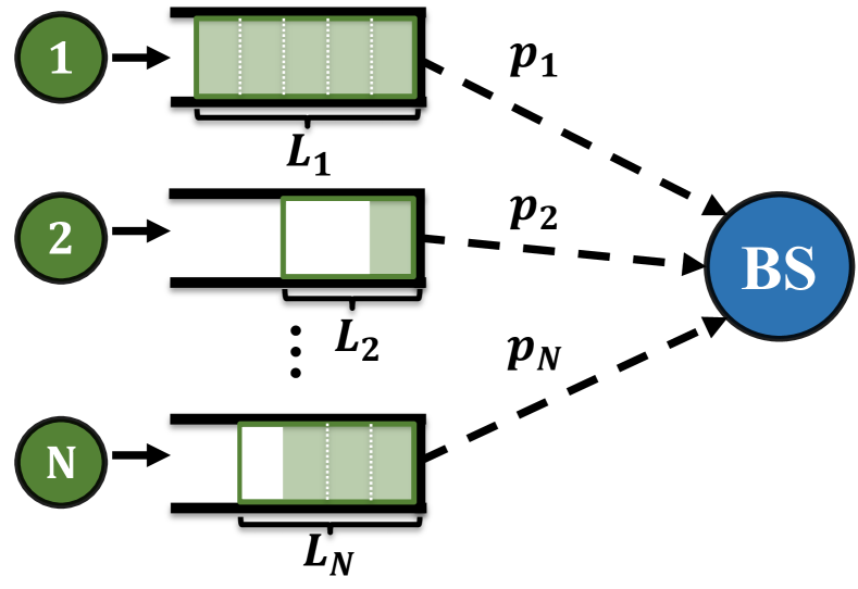
Figure 1: Network with $N$ sources transmitting information updates to a base station (BS). Sources generate updates over time and keep only the freshest update. Updates from source $i\in\{1,\ldots,N\}$ are composed of $L_{i}$ data packets. The BS selects one source at every time slot $t$ to transmit a single packet via its unreliable wireless link.

In this paper, we consider a network with multiple sources transmitting time-sensitive updates to a base station (BS), as illustrated in Fig. 1. We assume that information updates generated by source $i\in\{1,2,\ldots,N\}$ are composed of $L_{i}$ data packets. Further, we assume that, in each time slot, the BS can schedule one source to transmit a single data packet, and that these transmissions are unreliable. Our goal is to develop transmission scheduling policies that attempt to optimize information freshness in the network.

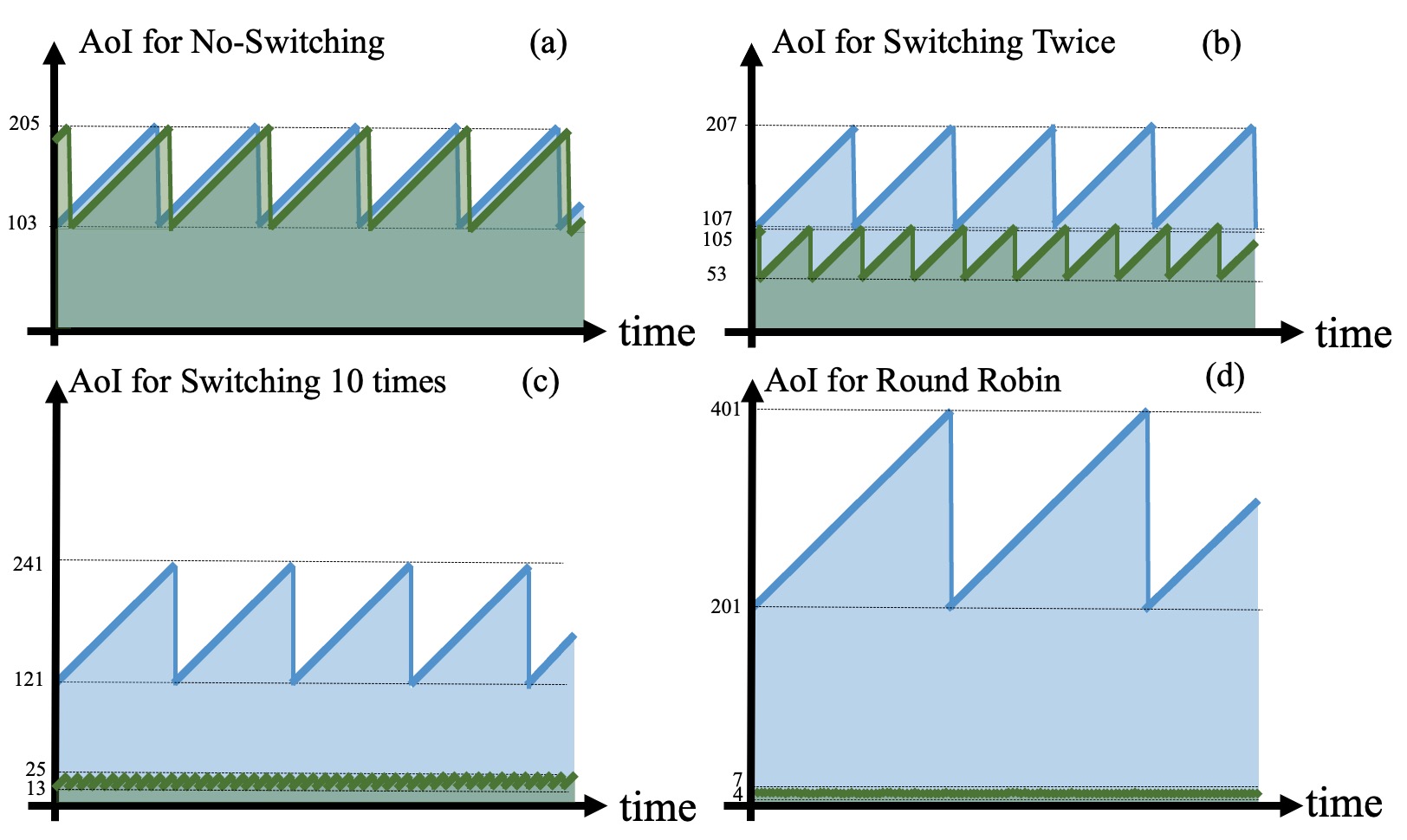
Figure 2: AoI evolution in a two-source network with reliable channels and sources 1 and 2 with update lengths $L_{1}=100$ and $L_{2}=2$, respectively. Each of the four plots are associated with a different scheduling policy: (a) no-switching; (b) switching twice during the update of source 1; (c) switching 10 times during the update of source 1; and (d) round robin. The average AoI is shown in Table I

TABLE I: Average AoI associated with the plots in Fig. 2.

Scheduling Policy	Average AoI
(a) No-Switching	154
(b) Switching Twice	118
(c) Switching 10 times	99
(d) Round Robin	153.25

Developing effective scheduling policies in networks with different update sizes is challenging. To illustrate this challenge, we consider a simple two-source network with reliable channels in which source 1 transmits large updates, each with $L_{1}=100$ packets, and source 2 transmits small updates, each with $L_{2}=2$ packets. In each time slot, only one source can be scheduled by the BS. In Fig. 2, we compare the AoI evolution associated with four scheduling policies: (a) no-switching policy, which delivers complete updates from sources 1 and 2 in turns; (b) switching twice policy, which periodically delivers two small updates from source 2 for every large update from source 1; (c) switching 10 times policy, which periodically delivers ten small updates for every large update; and (d) the round robin policy, which schedules packet transmissions from sources 1 and 2 in turns. Table I reports the average AoI achieved by the different policies, indicating that, even in small networks with reliable channels, judiciously accounting for the different update lengths can significantly improve AoI.

However, most scheduling policies proposed in prior works [9, 10, 11, 12, 13, 14, 15, 16, 17] are designed under the assumption that every successful transmission of a fresher packet to the destination leads to an AoI reduction, which is only true if $L_{i}=1,\forall i$, and can lead to poor AoI performance. Table I shows that the two policies that disregard the difference in update lengths, namely No-Switching and Round Robin, have an average AoI that is at least $54\%$ worse than Switching 10 times.

Main Contributions. In this paper, we address the problem of AoI optimization in wireless networks in which sources may have different update lengths. Our main contributions can be summarized as follows:

• We find the optimal schedulers for two classes of policies: (i) Switching Randomized Policies (SRP), in which the BS randomly selects a source for transmission in every slot $t$; and (ii) No-Switching Randomized Policies (NSRP), in which once the first packet of an update is successfully transmitted to the BS, the BS must continuously select the same source until the entire information update is delivered. We obtain closed-form analytical expressions for the AoI performance of SRP and NSRP. Using our universal lower bound, which generalized prior works [18, 19], we derive a constant factor optimality guarantee for the optimal SRP.

• We develop a novel low-complexity Max-Weight policy that makes scheduling decisions based on: AoI, system time, and remaining number of packets in the current update. We derive a constant factor optimality guarantee for the Max-Weight policy. To the best of our knowledge, this is the first policy with a constant factor optimality guarantee in terms of AoI for networks with different update lengths and unreliable channels.

• To derive performance guarantees, we propose a novel Lyapunov function and analysis. Traditional AoI-based Lyapunov functions and analysis are insufficient since there can be long periods of time when the AoI does not change despite successful packet deliveries (due to large update sizes and unreliable channels). We add notions of system time, waiting time, and throughput debt to our Lyapunov function and utilize these in Lyapunov drift analysis to obtain our performance bounds.

• We evaluate the impact of the network configuration and scheduling policy on AoI. Our numerical results show that, the performance of the Max-Weight policy is near optimal for a wide variety of network settings.

Related Work. The design of transmission scheduling policies that optimize the AoI in wireless networks has been extensively investigated (e.g., [9, 10, 11, 12, 13, 14, 15, 16, 17, 19, 20, 21, 22]). Various network configurations have been considered, including those with stochastic arrivals [9, 10], energy constraints [11, 12], throughput constraints [13, 14], and imperfect knowledge [15, 16, 17]. Most prior works [9, 10, 11, 12, 13, 14, 15, 16, 17] assume that each update consists of a single packet, while a few recent studies [8, 22, 19, 20, 21] considered networks with different update sizes. Most related to this paper are [19, 20, 21].

In [19], Li et al. consider networks with reliable channels and sources that generate updates with different sizes. They develop the Juventas scheduling policy based on the “AoI outage” defined as the difference between AoI and system time and provide performance guarantees under the assumption that each update can be fully delivered within one time slot. The interesting insights in [19] are limited to networks with reliable channels. Similarly, in [20], Tripathi et al. propose a low-complexity Whittle index resource allocation algorithm for networks with reliable channels and non-uniform update lengths. This algorithm assumes that complete updates must be transmitted before switching sources, and it lacks performance guarantees in terms of AoI. In [21], Zhou et al. study AoI minimization by jointly designing sampling and scheduling policies. They derive the Bellman equation, unveil interesting structural properties of the solution, apply linear decomposition method to decouple sources, and develop a structure-aware algorithm that solve the Bellman equation for each source in parallel to compute a sub-optimal policy. The proposed structure-aware algorithm has no performance guarantees and it has a computational complexity of $\mathcal{O}(\bar{h}^{2}L)$, where $\bar{h}$ is the imposed upper bound on the AoI and $L$ is the update length, which may limit its practical applicability.

In contrast, in this paper we consider wireless networks where sources generate updates of different lengths and the wireless channels are unreliable. We develop dynamic scheduling policies with constant factor optimality guarantees in terms of AoI. Further, our proposed scheduling schemes are low complexity - their complexity scales linearly with the number of sources and does not scale at all with the size of the updates $L$.

The remainder of this paper is organized as follows. In Sec. II, we describe the network model. In Sec. III, we derive a lower bound on the achievable AoI. In Sec. IV, we develop and analyze the optimal SRP and optimal NSRP. We also use the lower bound derived from earlier to prove performance guarantees for the optimal SRP and NSRP. In Sec. V, we develop and analyze the Max-Weight policy, and provide performance bounds. In Sec. VI, we provide detailed numerical results that illustrate the performance gains of our approach in a wide variety of network settings.

II Network Model

Consider a single-hop wireless network with a base station (BS) that receives time-sensitive updates from $N$ sources, as illustrated in Fig. 1. Let time be slotted, with slot index $t\in\{1,2,\ldots,T\}$, where $T$ denotes the time horizon. Each information update generated by source $i\in\{1,2,\ldots,N\}$ consists of $L_{i}$ data packets, where each packet can be entirely transmitted in one time slot. An information update is deemed to have been delivered successfully only after all $L_{i}$ data packets reach the BS. However, due to interference and capacity constraints, only one source can transmit in any given time slot, and the BS can receive at most one packet per slot, which may not constitute an entire update. These limitations necessitate the careful design of scheduling policies that account for AoI, the size of updates, and the number of packets remaining in queues. Next, we discuss the update generation process and packet transmission process in our system model.

Update Generation Process. Updates generated by each source $i$ are queued in a corresponding single update buffer queue. At any time slot, the queue contains all the packets that are remaining for transmission from the latest generated information update. Each source decides whether to generate a new update and place it in its buffer by looking at the number of packets remaining in the queue. Specifically, if the buffer is empty, then source $i$ generates a new update and places it in the buffer. Similarly, if the buffer is full, and the source is not currently transmitting, then it generates a new update and places it in the buffer. This generation policy ensures that the source always transmits the freshest available update, when it starts transmission. We assume that the update generation and transmission is non-preemptive, i.e. if a part of the update remains undelivered, then the source keeps the remainder of the current update in the buffer and does not replace it with a new update. Intuitively, this queuing discipline helps reduce the age of information by avoiding partial transmissions that do not reduce AoI, while ensuring that newly transmitted updates remain as fresh as possible.

Packet Transmission Process. In each slot $t$, the BS either idles or selects one source for transmission. Let $u_{i}(t)=1$ indicate that source $i$ is selected during slot $t$, and $u_{i}(t)=0$ otherwise. It follows that $\sum_{i=1}^{N}u_{i}(t)\leq 1,\forall t.$ The selected source attempts to transmit one packet from its queue to the BS over an unreliable wireless channel. Let $c_{i}(t)=1$ indicate that the channel from source $i$ to the BS is ON during slot $t$, and $c_{i}(t)=0$ indicates otherwise. The channel states $c_{i}(t)$ are i.i.d. over time and independent across different sources, with $\mathbb{P}(c_{i}(t)=1)=p_{i}\in(0,1]$ for all $i,t$.

Let $d_{i}(t)$ be an indicator such that $d_{i}(t)=1$ if source $i$ successfully transmits a packet in slot $t$, and 0 otherwise. A transmission is successful if the source is scheduled and the channel is ON, implying $d_{i}(t)=c_{i}(t)\,u_{i}(t),\forall i,t$. Since the BS does not know the channel states before making scheduling decisions, $u_{i}(t)$ and $c_{i}(t)$ are independent, which yields $\mathbb{E}[d_{i}(t)]=p_{i}\,\mathbb{E}[u_{i}(t)],\forall i,t$.

Without loss of generality, we assume that at the beginning of each slot $t$, the update generation occurs before packet transmission can start. Next, we introduce network performance metrics of interest and then formulate the AoI minimization problem.

Remaining Update Length. Let $L_{i}(t)\in\{1,2,\ldots,$ $L_{i}\}$ denote the number of packets remaining to be transmitted in source $i$’s queue at the beginning of slot $t$, after the update generation process. The evolution of $L_{i}(t)$ is given by

$$L_{i}(t+1)=\begin{cases}L_{i},&\text{if }d_{i}(t)=1\text{ and }L_{i}(t)=1,\\ L_{i}(t)-1,&\text{if }d_{i}(t)=1\text{ and }L_{i}(t)\neq 1,\\ L_{i}(t),&\text{if }d_{i}(t)=0.\end{cases}$$ (1)

The remaining update length $L_{i}(t)$ is critical for AoI tracking, as it determines the number of packet deliveries required before the AoI can be reduced.

System Time. The system time of the update in the queue of source $i$ in slot $t$ is defined as $z_{i}(t):=t-\tau^{S}_{i}(t)$, where $\tau^{S}_{i}(t)$ represents the time at which the update was generated (i.e., the “source timestamp”). The system time evolves as

$$z_{i}(t+1)=\begin{cases}1,&\text{if }d_{i}(t)=0\text{ and }L_{i}(t)=L,\\ &\text{or }d_{i}(t)=1\text{ and }L_{i}(t)=1,\\ z_{i}(t)+1,&\text{otherwise}.\end{cases}$$ (2)

System time $z_{i}(t)$ is crucial for tracking AoI, as it measures how fresh the update is before delivery.

Age of Information. Let $h_{i}(t):=t-\tau^{D}_{i}(t)$ be the AoI associated with source $i$ at the beginning of slot $t$, where $\tau^{D}_{i}(t)$ is the generation time of the last delivered update. The evolution of $h_{i}(t)$ is given by:

$$h_{i}(t+1)=\begin{cases}z_{i}(t)+1&\text{if }d_{i}(t)=1\text{ and }L_{i}(t)=1,\\ h_{i}(t)+1&\text{otherwise.}\end{cases}$$ (3)

We assume that $h_{i}(1)=1$, $z_{i}(1)=0,\forall i$, and $L_{i}(1)=L_{i},\forall i$.

Long-term Packet Throughput. The long-term packet throughput of source $i$ is given by

$$q_{i}=\lim_{T\rightarrow\infty}\frac{\mathbb{E}[D_{i}(T)]}{T},$$ (4)

where $D_{i}(T)=\sum^{T}_{t=1}d_{i}(t)$ is the total number of information updates delivered from source $i$ by the end of the time-horizon $T$. The shared and unreliable wireless channel restricts the set of feasible values of long-term throughput. By employing $\mathbb{E}[d_{i}(t)]=p_{i}\mathbb{E}[u_{i}(t)]$ and $\sum^{N}_{i=1}u_{i}(t)\leq 1$ into the definition of long-term throughput in (4), we obtain

$$\frac{\mathbb{E}[D_{i}(T)]}{T}=\frac{p_{i}\sum_{t=1}^{T}\mathbb{E}[u_{i}(t)]}{T}=\sum_{i=1}^{N}\frac{q_{i}}{p_{i}}\leq 1.$$ (5)

AoI minimization problem. The transmission scheduling policies considered in this paper are non-anticipative, which means that they do not use future information when making scheduling decisions. Let $\Pi$ represent the class of non-anticipative policies and let $\pi\in\Pi$ denote an arbitrary admissible policy. To capture the information freshness in a network employing policy $\pi\in\Pi$, we define the Expected Weighted Sum AoI (EWSAoI) in the limit as the time horizon $T$ grows to infinity as

$$\mathbb{E}[J^{\pi}]=\lim_{T\to\infty}\frac{1}{TN}\sum_{t=1}^{T}\sum_{i=1}^{N}\alpha_{i}\mathbb{E}[h_{i}^{\pi}(t)],$$ (6)

where $\alpha_{i}>0$ represents the priority of source $i$. We denote by $\pi^{*}\in\Pi$ the AoI-optimal policy that achieves minimum EWSAoI, namely

$\displaystyle\mathbb{E}\left[J^{*}\right]=\min_{\pi\in\Pi}\lim_{T\to\infty}$ $\displaystyle\frac{1}{TN}\sum_{t=1}^{T}\sum_{i=1}^{N}\alpha_{i}\mathbb{E}[h_{i}^{\pi}(t)],$ (7) s.t. $\displaystyle\sum_{i=1}^{N}u_{i}(t)\leq 1.$ (8)

where $\mathbb{E}\left[J^{*}\right]$ is the EWSAoI associate with policy $\pi^{*}$, and the expectation is with respect to the randomness in the channel state $c_{i}(t)$ and in scheduling decisions $u_{i}(t)$. Next, we derive a universal lower bound for the AoI minimization problem.

III Lower Bound

In this section, we derive a lower bound on the achievable EWSAoI under any admissible scheduling policy $\pi\in\Pi$. We first define waiting time and service time, then we characterize the EWSAoI in terms of these two quantities, and, finally, we derive the lower bound.

Waiting Time and Service Time. Let $K_{i}(T)$ denote the total number of delivered updates from source $i$ by the end of slot $T$ and let $m\in\{1,...,K_{i}(T)\}$ be the index of the delivered updates from source $i$. Let $t^{\prime}_{i}[m]$ denote the time slot in which the first packet of the $m$th delivered update is received, and let $t_{i}[m]$ denote the time slot in which the last packet of the $m$th delivered update is received. We define the waiting time of the $m$th update from source $i$ as $W_{i}[m]\;:=\;t^{\prime}_{i}[m]-t_{i}[m-1]$, which is the interval between the delivery of the last packet of the $(m-1)$th update and the delivery of the first packet of the $m$th update. Similarly, the service time of the $m$th update for source $i$ is defined as $S_{i}[m]\;:=\;t_{i}[m]-t^{\prime}_{i}[m]$, which is the interval between the delivery of the first and last packets of the $m$th update. We assume that $t_{i}[0]=0$, $W_{i}[0]=0$, and $S_{i}[0]=0$ for all $i$.

For a set of values $\mathbf{x}$, let $\bar{\mathbb{M}}[\mathbf{x}]$ denote the sample mean. The time horizon $T$ is omitted in the notation $\bar{\mathbb{M}}[\cdot]$ for simplicity. Using this operator, the sample mean of $W_{i}[m]$ and $S_{i}[m]$ for a fixed source $i$ is given by

$$\bar{\mathbb{M}}\bigl{[}W_{i}[m]\bigl{]}\;:=\;\frac{1}{K_{i}(T)}\sum_{m=1}^{K_{i}(T)}W_{i}[m],$$ (9)

$$\bar{\mathbb{M}}\bigl{[}S_{i}[m]\bigl{]}\;:=\;\frac{1}{K_{i}(T)}\sum_{m=1}^{K_{i}(T)}S_{i}[m].$$ (10)

Proposition 1.

The infinite-horizon Weighted Sum AoI achieved by scheduling policy $\pi$, i.e. $J^{\pi}$, can be written as

$$J^{\pi} =\lim_{T\rightarrow\infty}\sum_{i=1}^{N}\frac{\alpha_{i}}{N}\Biggl{(}\frac{\bar{\mathbb{M}}\bigl{[}(W_{i}[m]+S_{i}[m])^{2}\bigr{]}}{2\,\bar{\mathbb{M}}\bigl{[}W_{i}[m]+S_{i}[m]\bigr{]}}$$ (11)

$$\quad+\;\frac{\bar{\mathbb{M}}\bigl{[}S_{i}[m-1]\,(W_{i}[m]+S_{i}[m])\bigr{]}}{\bar{\mathbb{M}}\bigl{[}W_{i}[m]+S_{i}[m]\bigr{]}}\;+\;1\Biggr{)},$$

where $W_{i}[m]$ and $S_{i}[m]$ are the waiting time and service time of the $m$th update from source $i$.

Proof.

Using a sample path argument, we compute the sum of AoI during each update, and take the average over time by rewriting the time horizon $T$ as the sum of waiting and service times. By omitting zero-order terms, we obtain (11). Detailed derivations are provided in Appendix A.∎

Remark 2.

Equation (11) holds for any scheduling policy $\pi\in\Pi$ and generalizes known results for the single-packet case [13] to the scenario where each update may contain multiple packets. The first term on the RHS of (11) depends on both the waiting time and service time. The second term depends on the previous update’s service time and the sum of the current update’s waiting time and service time. Intuitively, to minimize AoI, the scheduling policy should attempt to deliver packets from a source that currently has high waiting time and high service time, especially the latter.

Based on Proposition 1, we now establish a universal lower bound on the achievable AoI.

Theorem 3.

For a network with parameters $\{N,\alpha_{i},p_{i},L_{i}\}$, the following bound holds for all admissible policies $\pi\in\Pi$:

$$L_{B}=\frac{1}{2N}\Biggl{(}\sum_{i=1}^{N}\sqrt{\frac{\alpha_{i}\,L_{i}}{p_{i}}}\Biggr{)}^{2}+\sum_{i=1}^{N}\alpha_{i}\leq\mathbb{E}[J^{\pi}],$$ (12)

Proof.

Applying Jensen Inequality and $S_{i}[m-1](W_{i}[m]+S_{i}[m])>0,\forall i,m,$, we obtain a lower bound on (11). Then, by using Cauchy-Schwarz Inequality to solve the optimization problem with respect to throughput of each sources yields (12). Detailed derivations are provided in Appendix B.∎

IV Randomized Policies

In this section, we discuss two classes of randomized scheduling policies: Switching Randomized Policies, in which the BS randomly selects a source for transmission in every slot $t$; and No-Switching Randomized Policies, in which once the first packet of an update is successfully transmitted to the BS, the BS must continuously select the same source until the entire information update is delivered. In Sec. IV-C, we compare the performance of these two classes of randomized policies in symmetric and non-symmetric networks.

IV-A Switching Randomized Policies (SRP)

Let $\Pi^{s}_{r}$ denote the class of SRPs. A BS running a policy $s\in\Pi^{s}_{r}$ operates as follows: in each slot $t$, the BS selects source $i$ with scheduling probability $\mu^{s}_{i}\in(0,1]$, where the probabilities satisfy $\sum_{i=1}^{N}\mu^{s}_{i}\leq 1.$ If source $i$ is selected during slot $t$, then it transmits a packet to the BS. SRPs select sources at random, without taking into account the current AoI $h_{i}(t)$, system time $z_{i}(t)$, nor the number of remaining packet $L_{i}(t)$ at each source. Each policy $s$ is fully characterized by the set of scheduling probabilities $\{\mu^{s}_{i}\}^{N}_{i=1}$. Note that under an SRP, packets from different sources are interleaved between one another, it is not necessary for all packets belonging to an update to be delivered continuously.

Next, we obtain the optimal SRP and provide performance guarantees for it in terms of AoI. Specifically, Proposition 4 provides the EWSAoI associated with an arbitrary SRP $s\in\Pi_{s}$ and Theorem 5 characterizes the optimal SRP $S$ and its performance guarantee.

Proposition 4.

For a network with parameters $\{N,\alpha_{i},p_{i},L_{i}\}$ and any SRP $s\in\Pi^{s}_{r}$ characterized by $\{\mu^{s}_{i}\}_{i=1}^{N}$, the corresponding EWSAoI is given by

$$\mathbb{E}[J^{s}]=\frac{1}{N}\sum_{i=1}^{N}\alpha_{i}\left(\frac{3L_{i}-1}{2p_{i}\mu^{s}_{i}}+1\right).$$ (13)

Proof.

First, we take the expectation of (11) to obtain an expression for the EWSAoI. Then, we substitute the first and second moments of the waiting time and service times – which follow a negative binomial distribution [23] – to obtain (13). Detailed derivations are provided in Appendix C.∎

From (13), we can obtain the optimal SRP $S$ by solving

$$\min_{\{\mu^{s}_{i}\}_{i=1}^{N}}\sum_{i=1}^{N}\alpha_{i}\biggl{(}\frac{3\,L_{i}-1}{2\,p_{i}\,\mu^{s}_{i}}\biggr{)}\quad\text{s.t.}\quad\sum_{i=1}^{N}\mu^{s}_{i}\;\leq\;1.$$ (14)

Theorem 5.

For a network with parameters $\{N,\alpha_{i},p_{i},L_{i}\}$, let $S\in\Pi^{s}_{r}$ be the optimal SRP. Its scheduling probabilities $\{\mu^{S}_{i}\}_{i=1}^{N}$ are given by

$$\mu^{S}_{i}\;=\;\frac{\sqrt{\frac{\alpha_{i}\,(3\,L_{i}-1)}{2\,p_{i}}}}{\sum_{j=1}^{N}\sqrt{\frac{\alpha_{j}\,(3\,L_{j}-1)}{2\,p_{j}}}},\quad\forall i.$$ (15)

The associated EWSAoI is given by

$$\mathbb{E}[J^{S}]\;=\;\frac{1}{N}\sum_{i=1}^{N}\alpha_{i}\;+\;\frac{1}{N}\left(\sum_{i=1}^{N}\sqrt{\tfrac{\alpha_{i}\,(3\,L_{i}-1)}{2\,p_{i}}}\right)^{2}.$$ (16)

which satisfies

$$L_{B}\;\leq\;\mathbb{E}[J^{S}]\;\leq\;\rho^{S}\,L_{B},$$ (17)

where $L_{B}$ is the lower bound from Theorem 3 and the optimality ratio $\rho^{S}$ is

$$\rho^{S}=\frac{\frac{1}{N}\Bigl{(}\sum_{i=1}^{N}\sqrt{\tfrac{\alpha_{i}(3L_{i}-1)}{2p_{i}}}\Bigr{)}^{2}+\frac{1}{N}\sum_{i=1}^{N}\alpha_{i}}{\frac{1}{2N}(\sum_{i=1}^{N}\sqrt{\frac{\alpha_{i}L_{i}}{p_{i}}})^{2}+\frac{1}{N}\sum_{i=1}^{N}\alpha_{i}}$$ (18)

Proof.

To solve (14) we apply Cauchy-Schwarz Inequality and immediately obtain the optimal SRP in (15). Substituting (15) into (13) yields the EWSAoI expression in (16). Comparing (16) and (12) gives (17) and (18). Detailed derivations are provided in Appendix D.∎

Notice that when $L_{i}=1,\forall i$, the optimal SRP coincides with that in [18] and achieves an optimality ratio of $\rho^{S}=2$. In the more realistic and general case when update lengths $\{L_{i}\}_{i=1}^{N}$ are arbitrary, the optimal SRP attains an optimality ratio in the range $\rho^{S}\in[2,3)$.

IV-B No-Switching Randomized Policies (NSRP)

We denote by $\Pi^{ns}_{r}$ the class of NSRPs. In contrast to SRPs, NSRPs $ns\in\Pi^{ns}_{r}$ do not switch sources between updates. Specifically, once the first packet of an update is successfully transmitted (i.e., $d_{i}(t)=1$ and $L_{i}(t)=L_{i}$), the BS continues selecting the same source for transmission until the update delivery is complete. In the slot following the successful transmission of the last packet of an update, the BS selects any source $i$ with scheduling probability $\mu^{ns}_{i}\in(0,1]$, with $\sum_{i=1}^{N}\mu^{ns}_{i}\leq 1$. Random selection of sources, according to $\{\mu^{ns}_{i}\}_{i=1}^{N}$, continues until the first packet is successfully transmitted. Intuitively, NSRPs reduce the service time $S_{i}[m]$ by continuously transmitting an entire update from a single source, which is in line with the discussion in Remark 2.

NSRPs do not consider the current AoI $h_{i}(t)$ nor the system time $z_{i}(t)$. However, NSRPs behave differently in case $L_{i}(t)=L_{i}$, when scheduling decisions are randomized $\{\mu^{ns}_{i}\}_{i=1}^{N}$, and in case $L_{i}(t)<L_{i}$, when scheduling decisions are deterministic. Each policy $ns$ is fully characterized by the set of scheduling probabilities $\{\mu^{ns}_{i}\}_{i=1}^{N}$. Proposition 6 provides an expression for the EWSAoI associated with an arbitrary NSRP $ns\in\Pi^{ns}_{r}$.

Proposition 6.

For a network with parameters $\{N,\alpha_{i},p_{i},L_{i}\}$ and an arbitrary NSRP $ns\in\Pi^{ns}_{r}$ with scheduling probabilities $\{\mu^{ns}_{i}\}_{i=1}^{N}$, the EWSAoI is given by:

$$\mathbb{E}[J^{ns}] =\sum_{i=1}^{N}\frac{\alpha_{i}}{N}\Biggl{[}\frac{\mu^{ns}_{i}p_{i}}{\sum^{N}_{j=1}\mu^{ns}_{j}L_{j}}\Biggl{(}\frac{\mathbb{E}[W^{2}_{i}]+\mathbb{E}[S^{2}_{i}]}{2}$$ (19)

$$+\left(\frac{L_{i}-1}{p_{i}}\right)^{2}+2\mathbb{E}[W^{2}_{i}]\left(\frac{L_{i}-1}{p_{i}}\right)\Biggl{)}+1\Biggr{]}.$$

Here, $\mathbb{E}[S_{i}^{2}]$, $\mathbb{E}[W_{i}]$, and $\mathbb{E}[W_{i}^{2}]$ denote the second moment of the service time, the first moment of the waiting time, and the second moment of the waiting time, respectively. The term $\mathbb{E}[Y_{i}^{2}]$ represents the second moment of the number of time slots between two consecutive transmissions from source $i$. These quantities are given by

$$\mathbb{E}[S^{2}_{i}] =\frac{(L_{i}-1)(L_{i}-p_{i})}{p_{i}^{2}},$$ (20)

$$\mathbb{E}[W_{i}] =\frac{\sum^{N}_{j=1}\mu^{ns}_{j}L_{j}-\mu^{ns}_{i}(L_{i}-1)}{\mu^{ns}_{i}p_{i}},$$ (21)

$$\mathbb{E}[W_{i}^{2}] =\frac{1}{1-\sum_{j}\mu^{ns}_{j}+p_{i}\mu^{ns}_{i}}\Biggl{[}\mu^{ns}_{i}\left(1+2(1-p_{i})\mathbb{E}[W_{i}]\right)$$

$$+\sum_{j\neq i}\mu^{ns}_{j}\left(\mathbb{E}[Y_{j}^{2}]+2L_{j}\mathbb{E}[W_{i}]\right)\Biggl{]},$$ (22)

$$\mathbb{E}[Y_{i}^{2}] =2L_{i}-1+\frac{(L_{i}-1)(L_{i}-p_{i})}{p_{i}}.$$ (23)

Proof.

First, we take the expectation of (11) to obtain an expression for the EWSAoI. For a network employing a NSRP, the service time follows a negative binomial distribution [23] and the waiting time can be modeled as a Markov chain, from which its first and second order moments are derived via recurrence time analysis. Substituting these results into the EWSAoI expression yields (19). Detailed derivations are provided in Appendix E.∎

From the expression for the EWSAoI in (19), we can find the optimal scheduling probabilities $\{\mu^{NS}_{i}\}_{i=1}^{N}$ by solving the optimization problem below:

$$\min_{\{\mu^{ns}_{i}\}_{i=1}^{N}}\mathbb{E}[J^{ns}],\quad\text{s.t.}\sum_{i=1}^{N}\mu^{ns}_{i}\leq 1$$ (24)

The complex expression for the EWSAoI in (19) does not lend itself for a closed-form solution for the optimal scheduling probabilities $\{\mu^{NS}_{i}\}_{i=1}^{N}$. However, (24) is a convex optimization problem that can be solved numerically. In Sec. VI, we use a numerical solver to obtain the values of $\{\mu^{NS}_{i}\}_{i=1}^{N}$.

IV-C Comparison of Randomized Policies

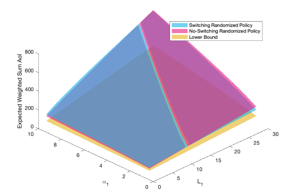
Figure 3: Simulation results of two-source networks with varying weight $\alpha_{1}\in\{1,2,\dots,10\}$ and update length $L_{1}\in\{2,4,\dots,30\}$, while $\alpha_{2}=10$, $L_{2}=2$, and $p_{1}=p_{2}=0.5$ remain fixed.

We now compare the performance of the optimal SRP and the optimal NSRP in symmetry and non-symmetric networks.

Corollary 7.

Consider a symmetric network with channel reliabilities $p_{i}=p\in(0,1]$, update lengths $L_{i}=L>0$, and weights $\alpha_{i}=\alpha>0$ for all $i$. Let $\mathbb{E}[J^{NS}]$ and $\mathbb{E}[J^{S}]$ be the EWSAoI achieved by the optimal no-switching and the optimal switching randomized policies, respectively. Then,

$$\mathbb{E}[J^{NS}]\leq\mathbb{E}[J^{S}]$$ (25)

This corollary demonstrates that in symmetric networks the no-switching approach consistently outperforms the switching approach by leveraging continuous transmissions for each source, resulting in lower service times for the selected source, and thus lower EWSAoI.

Figure 3 compares the EWSAoI of the optimal SRP and NSRP in a non-symmetric two-source network with fixed channel reliabilities $p_{1}=p_{2}=0.5$. The parameters for source 1 vary over $\alpha_{1}\in\{1,2,\dots,10\}$ and $L_{1}\in\{2,4,\dots,30\}$, while source 2 has fixed $\alpha_{2}=10$ and $L_{2}=2$.

Remark 8.

As can be seen in Fig. 3, in highly asymmetric networks, the optimal SRP can significantly outperform the optimal NSRP in terms of the EWSAoI. This result is in line with Fig. 2 and Table I which showed switching policies that outperformed the no switching policy by more than $54\%$. Intuitively, under a NSRP, once transmission begins for a source with a large update length, the AoI for other sources continues to rise until the update is fully delivered. In these cases, switching to another source with low update length earlier could reduce the average AoI, as seen in Fig. 2, but the no-switching approach prevents such adaptive flexibility.

V Max-Weight Policy

In this section, we develop a Max-Weight policy [24] designed to reduce the expected drift of a suitably constructed Lyapunov function at every time slot $t$. The Lyapunov function outputs a nonnegative scalar that is high when the network is in undesirable states. Prior works including [18, 9, 13] utilized Lyapunov functions and one-slot Lyapunov drift analysis that focused on AoI $h_{i}(t)$ and system times $z_{i}(t)$. While this approach is suitable for networks with $L_{i}=1,\forall i$ in which every packet transmission may lead to a reduction of AoI in the next time slot. This approach is not suitable for networks with large $L_{i}$ when the AoI reduction (i.e., the reward) may come in the distant future and may depend on the (stochastic) outcome of future scheduling decisions. This time-dependency and complexity also makes multi-slot Lyapunov drift analysis [24] unsuitable.

To address this challenge, we draw inspiration from Remark 2 to define a novel Lyapunov function that incorporates waiting time, “optimistic” service time, and throughput debt [25], and is amenable to one-slot Lyapunov drift analysis. Before developing the Max-Weight policy, we introduce the throughput debt, the proposed Lyapunov function, and the corresponding one-slot Lyapunov drift.

Throughput Debt. Let $x_{i}(t)$ denote the throughput debt associated with source $i$ at the beginning of slot $t$. The throughput debt is defined as $x_{i}(t+1)=t\bar{q}_{i}-\sum_{\tau=1}^{t}d_{i}(\tau)$, where $\bar{q}_{i}$ is the long-term throughput target. The value of $t\bar{q}_{i}$ can be interpreted as the minimum number of packets that source $i$ should have delivered by slot $t+1$ and $\sum_{\tau=1}^{t}d_{i}(\tau)$ is the total number of packets actually delivered. Let the positive part of the throughput debt be $x^{+}_{i}(t)=\max\{x_{i}(t);0\}$. A large debt $x^{+}_{i}(t)$ indicates that source $i$ is lagging behind in terms of throughput. Notice that strong stability of the process $x^{+}_{i}(t)$, namely

$$\lim_{T\rightarrow\infty}\frac{1}{T}\sum_{t=1}^{T}\mathbb{E}[x^{+}_{i}(t)]<\infty$$ (26)

is sufficient to establish that the long-term throughput is larger than the target, i.e., $q_{i}\geq\bar{q}_{i}$. [26, Theorem 2.8]

Lyapunov Function. We propose the following Lyapunov function

$$\mathcal{L}(t) =\sum_{i=1}^{N}\beta_{i}\left[h_{i}(t)-z_{i}(t)\right]^{2}+\sum_{i=1}^{N}\gamma_{i}\left[z_{i}(t)+L_{i}(t)\right]^{2}$$ (27)

$$+\sum_{i=1}^{N}\frac{V}{2}\left[x_{i}^{+}(t)\right]^{2}$$

Notice that $h_{i}(t)-z_{i}(t)$ and $z_{i}(t)+L_{i}(t)$ capture the waiting time and an “optimistic” service time of the information update currently in source $i$, respectively. The service time is optimistic as it assumes that all remaining packets will take one slot to be delivered. The positive hyper-parameters $\beta_{i}$, $\gamma_{i}$, and $V$ are used to tune the Max-Weight policy to different network configurations. From Remark 2, we know that service time contributes more to the EWSAoI than waiting time, thus, $\gamma_{i}$ should be set to a higher value than $\beta_{i}$.

One-slot Lyapunov Drift. Let the network state observed by the BS at the beginning of slot $t$ be $\mathbb{S}(t):=\{h_{i}(t),z_{i}(t),L_{i}(t),x_{i}(t)\}_{i=1}^{N}$. The one-slot Lyapunov drift is defined as

$$\Delta\left(\mathbb{S}(t)\right):=\mathbb{E}\left[\mathcal{L}(t+1)-\mathcal{L}(t)|\mathbb{S}(t)\right]$$ (28)

By substituting the evolution of $L_{i}(t)$, $z_{i}(t)$, and $h_{i}(t)$ from (1), (2) and (3), respectively, into the drift expression in (28) and performing algebraic manipulations, we obtain an upper bound on $\Delta\bigl{(}\mathbb{S}(t)\bigr{)}$. The resulting bound is expressed in (29)–(31), with detailed steps provided in Appendix F.

$$\Delta\left(\mathbb{S}(t)\right)\leq B(t)-\sum_{i=1}^{N}p_{i}\mathbb{E}\left[u_{i}(t)|\mathbb{S}(t)\right]C_{i}(t)$$ (29)

where

$$B(t)= \sum_{i=1}^{N}\beta_{i}\mathbb{I}_{L_{i}(t)=L}\left[2h_{i}(t)-1\right]+V\left[x^{+}_{i}(t)\bar{q}_{i}+\frac{1}{2}\right]$$ (30)

$$+ \sum_{i=1}^{N}\gamma_{i}\mathbb{I}_{L_{i}(t)>1}\left[2\left(z_{i}(t)+L_{i}(t)\right)-1\right],$$

$$C_{i}(t) =\beta_{i}\mathbb{I}_{L_{i}(t)=L}\left[2h_{i}(t)-1\right]$$ (31)

$$+\beta_{i}\mathbb{I}_{L_{i}(t)=1}\left[h_{i}^{2}(t)-2h_{i}(t)z_{i}(t)\right]$$

$$+\gamma_{i}\mathbb{I}_{L_{i}(t)>1}\left[2z_{i}(t)+2L_{i}(t)-1\right]$$

$$+\gamma_{i}\mathbb{I}_{L_{i}(t)=1}\left[\left(z_{i}(t)+2\right)^{2}-\left(L_{i}+1\right)^{2}\right]+Vx^{+}(t).$$

The values of $B(t)$ and $C_{i}(t)$ can be easily calculated by any admissible policy and thus can be used for making scheduling decisions in real-time. The remaining update length $L_{i}(t)$ appears in (29)–(31) due to the dependence on evolution of $z_{i}(t)$ and $h_{i}(t)$ specified in (2) and (3).

Max-Weight policy. To minimize the upper bound (29), the Max-Weight (MW) policy selects, in each slot $t$, the source with highest value of $C_{i}(t)$, with ties being broken arbitrarily. Intuitively, by minimizing the one-slot Lyapunov drift, the Max-Weight policy will jointly minimize the waiting time and service time, resulting in low EWSAoI.

Theorem 9 provides a constant factor optimality guarantee for the MW policy. Before introducing Theorem 9, we define the long-term throughput associated with the lower bound in Theorem 3 (for details, please refer to the proof of Theorem 3)

$$q_{i}^{L_{B}}=\frac{\sqrt{\frac{\alpha_{i}\,L_{i}\,p_{i}}{2}}}{\sum_{j=1}^{N}\sqrt{\frac{\alpha_{j}\,L_{j}}{2\,p_{j}}}}$$ (32)

Theorem 9.

For a network with parameters $\{N,\alpha_{i},p_{i},L_{i}\}$, by choosing the constants $\beta_{i}=\frac{\alpha_{i}}{q_{i}^{L_{B}}},\gamma_{i}=\frac{\alpha_{i}}{q_{i}^{L_{B}}\sqrt{p_{i}}}$ and $\bar{q}_{i}=q^{L_{B}}_{i}-\epsilon$, where $\epsilon\rightarrow 0$, the optimality ratio of Max-Weight policy is such that

$$\rho=6+\frac{\sqrt{\varPsi}}{NL_{B}}$$ (33)

where

$$\varPsi= \left(\sum_{i=1}^{N}\alpha_{i}\right)\Biggl{(}\sum_{i=1}^{N}\frac{\alpha_{i}}{\sqrt{p_{i}}}\Bigl{[}5\frac{L^{2}_{i}\sqrt{p_{i}}}{\bar{q}^{2}_{i}}-\frac{L_{i}}{\bar{q}_{i}}$$ (34)

$$-\frac{L_{i}\sqrt{p_{i}}}{\bar{q}_{i}}+2\frac{L^{2}_{i}}{\bar{q}^{2}_{i}}+2\frac{L_{i}^{2}}{\bar{q}_{i}}\Bigl{]}\Biggl{)}$$

Proof.

First, we prove that if there exists a SRP $s$ satisfying $p_{i}\mu^{s}_{i}\geq\bar{q}_{i}$ for all $i$, then the MW policy also satisfies the throughput targets $\{\bar{q}_{i}\}_{i=1}^{N}$. Next, we perform algebraic manipulations to further bound the inequality in (29). We emphasize that, due to the dependency on $L_{i}(t)$, these algebraic manipulations departed from the traditional Lyapunov drift analysis commonly found in prior works including [18, 9, 13]. Finally, by comparing MW with the Lower Bound, we obtain (33). Detailed derivations are provided in Appendix G.∎

Remark 10.

The first term in $\varPsi$ scales as $\mathcal{O}(N)$, while the second term scales as $\mathcal{O}(N^{3})$ due to $1/\bar{q}_{i}$ being $\mathcal{O}(N)$. Consequently, $\sqrt{\varPsi}$ scales as $\mathcal{O}(N^{2})$, matching the scaling of $NL_{B}$. Hence, the optimality guarantee of the MW policy is bounded by a constant, irrespective of the network size $N$.

Numerical results in Sec VI show that MW outperforms both optimal SRP and optimal NSRP in every network configuration simulated. However, by comparing Theorems 9 and 5, it might seem that the optimal SRP yields a better performance than MW. This is because the analysis associated with MW is significantly more challenging, leading to an optimality ratio $\rho^{MW}$ that is looser than $\rho^{S}$. To the best of our knowledge, these are the first policies with a constant factor optimality guarantee in terms of AoI for networks with different update lengths and unreliable channels.

VI Simulation Results

In this section, we evaluate the performance of several scheduling policies in terms of their EWSAoI. Specifically, we compare the following policies: the optimal SRP proposed in Section IV-A. the optimal NSRP proposed in Section IV-B; the Greedy policy in which the BS selects the source with the highest $h_{i}(t)$ in each slot $t$; the Max-Weight policy for $L=1$ (MWL1) proposed in [18] in which the BS selects the source with highest value of $\sqrt{\alpha_{i}p_{i}}h_{i}(t)$ in each slot $t$; and the Max-Weight policy proposed in Section V. Their performance is benchmarked against the lower bound derived in Sec. III.

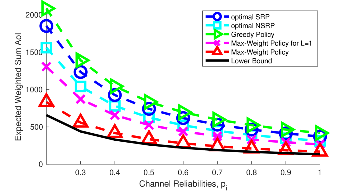
Figure 4: Simulation results for networks with varying channel reliabilities. The network comprises $N=10$ sources equally divided into Class 1 with $\alpha_{i}=5$ and $L_{i}=2$ and Class 2 with $\alpha_{i}=1$ and $L_{i}=50$. Channel reliabilities vary over $p_{i}\in\{0.2,\,0.15,\,\ldots,\,1\}$ for all sources.

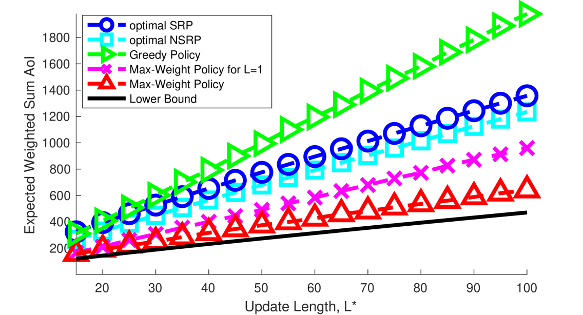
Figure 5: Simulation results for networks with varying update lengths. The network comprises $N=10$ sources equally divided into Class 1 with $\alpha_{i}=5$, $p_{i}=0.8$, and $L_{i}=2$ and Class 2 with $\alpha_{i}=1$ and $p_{i}=0.4$. Update lengths for Class 2 are parameterized as $[L^{*}-2,\,L^{*}-1,\,L^{*},\,L^{*}+1,\,L^{*}+2]$ with $L^{*}\in\{15,\,20,\,\ldots,\,100\}$.

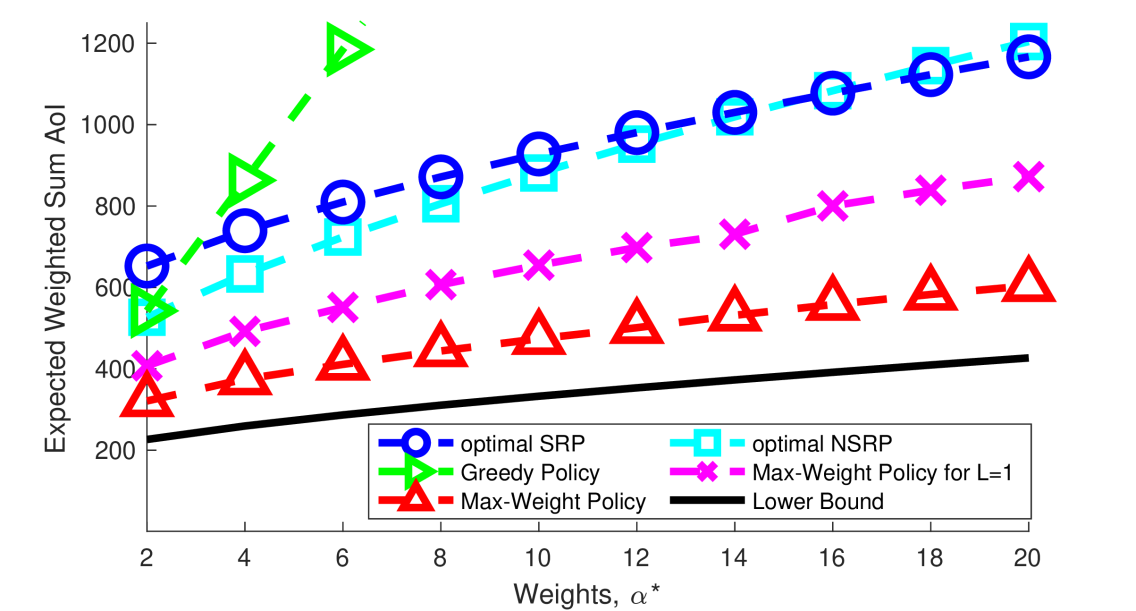
Figure 6: Simulation results for networks with varying weights. The network comprises $N=10$ sources equally divided into Class 1 with variable priorities $\alpha_{i}\in\{2,\,4,\,\ldots,\,20\}$ with fixed $L=2$ and $p_{i}=0.8$, and Class 2 sources have fixed parameters $\alpha_{i}=1$, $L_{i}=50$, and $p_{i}=0.4$.

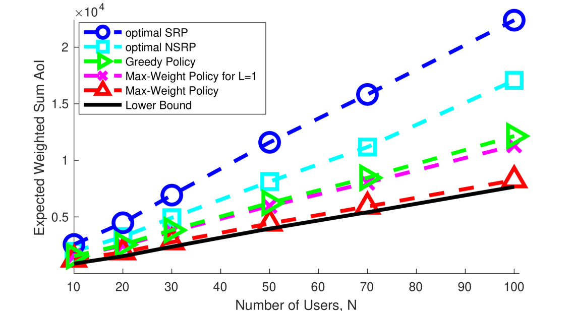
Figure 7: Simulation results for networks with a varying number of sources. The network comprises $N$ sources with $N\in\{10,20,30,50,70,100\}$. For each source, the weight is drawn from $\alpha_{i}\sim U[1,10]$, the channel reliability from $p_{i}\sim U[0.5,1]$, and each source is equally likely to belong to Class 1 (with $L_{i}\sim U[2,5]$) or Class 2 (with $L_{i}\sim U[20,100]$).

We consider two types of sources in our simulations: Class 1 sources are characterized by high weight $\alpha_{i}$ and small update length $L_{i}$; and Class 2 sources with low weight $\alpha_{i}$ and large update length $L_{i}$.

In Figures 4, 5, and 6, we consider networks with $N=10$ sources, equally divided into five Class 1 and five Class 2 sources. In Fig. 4, Class 1 sources are configured with a priority $\alpha_{i}=5$ and a fixed update length $L_{i}=2$, while Class 2 sources have $\alpha_{i}=1$ and $L_{i}=50$; in this setup, the channel reliabilities for all sources vary over the set $p_{i}\in\{0.2,0.15,\ldots,1\}$. In Fig. 5, the parameters for Class 1 sources remain the same ($\alpha_{i}=5$, $p_{i}=0.8$, $L_{i}=2$), and for Class 2 sources, while the priority is fixed at $\alpha_{i}=1$ and the channel reliability at $p_{i}=0.4$, the update lengths vary as $[L^{*}-2,\,L^{*}-1,\,L^{*},\,L^{*}+1,\,L^{*}+2]$ with $L^{*}$ taking values from $\{15,\,20,\,\ldots,\,100\}$. In Fig. 6, Class 1 sources have variable priorities $\alpha_{i}^{*}\in\{2,\,4,\,\ldots,\,20\}$ with $p_{i}=0.8$ and $L_{i}=2$, while Class 2 sources have $\alpha_{i}=1$, $p_{i}=0.4$, and $L_{i}=50$.

In Fig. 7, we simulate networks with the number of sources $N$ varying over $\{10,20,30,50,70,100\}$. Moreover, each source is equally likely to belong to either Class 1 or Class 2. Class 1 sources have an update length $L_{i}\sim U[2,5]$, while Class 2 sources have $L_{i}\sim U[20,100]$. For each source, the weight $\alpha_{i}\sim U[1,10]$ and the channel reliability $p_{i}\sim U[0.5,1]$.

Our results clearly demonstrate the superior performance of the Max-Weight policy. Figures 4, 5, and 6 show that the Max-Weight policy achieves near-optimal performance across various scenarios. In particular, Max-Weight policy consistently outperforms MWL1 especially in networks with non-symmetric update lengths, we observe that EWSAoI improves by 57$\%$ in Fig 4, 30$\%$ in Fig 5, and 33$\%$ in Fig. 6 in average. Moreover, Fig. 7 indicates that the performance of the Max-Weight policy remains robust as the network size increases.

VII Conclusion

In this paper, we considered a single-hop wireless network with a number of nodes transmitting time-sensitive updates to a Base Station over unreliable channels, where each updates consists of multiple packets. We addressed the problem of minimizing the Expected Weighted Sum AoI of the network with large updates. Three low-complexity scheduling policies were developed: optimal SRP, optimal NSRP, and Max-Weight policy. The performance of each policy was evaluated both analytically and through simulation. The Max-Weight policy demonstrated the best performance in terms of AoI. Interesting extensions include consideration of jointly designing the sampling and scheduling algorithm, general non-linear functions of AoI, fairness of AoI among the different sources with different update sizes, and distributed scheduling schemes.

Appendix A Proof of Propsition 1

Propsition 1. The infinite-horizon Weighted Sum AoI achieved by scheduling policy $\pi$, namely $J^{\pi}$, can be written as

$$J^{\pi}=\lim_{T\rightarrow\infty}\sum_{i=1}^{N}\frac{\alpha_{i}}{N}\Biggl{[}\frac{\bar{\mathbb{M}}\bigl{[}(W_{i}[m]+S_{i}[m])^{2}\bigr{]}}{2\,\bar{\mathbb{M}}\bigl{[}W_{i}[m]+S_{i}[m]\bigr{]}}+\frac{\bar{\mathbb{M}}\bigl{[}S_{i}[m-1]\,(W_{i}[m]+S_{i}[m])\bigr{]}}{\bar{\mathbb{M}}\bigl{[}W_{i}[m]+S_{i}[m]\bigr{]}}+1\Biggr{]},$$ (35)

where $W_{i}[m]$ and $S_{i}[m]$ are the waiting time and service time of the $m$th update for destination $i$.

Proof.

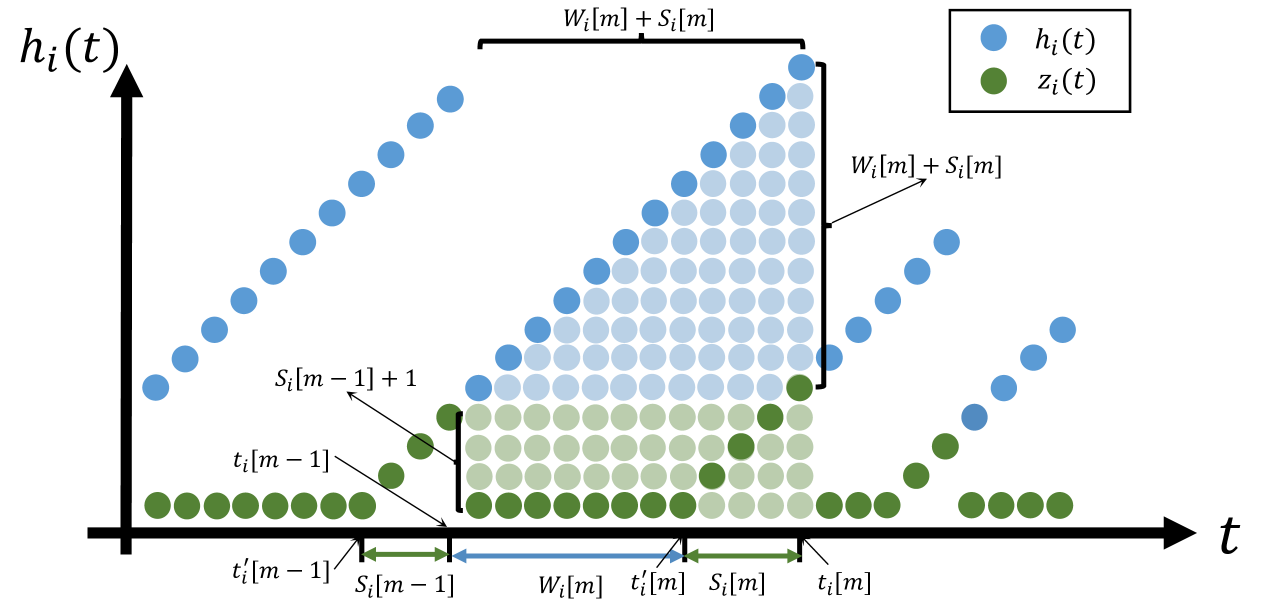
Figure 8: A sample path of AoI Evolution.

Consider a network operating under policy $\pi$ over a time horizon $T$. Let $\Omega$ be the associated sample space, and let $\omega\in\Omega$ denote a sample path, as shown in Fig. 8. Recall that $K_{i}(T)$ is the total number of updates delivered to destination $i$ by the end of slot $T$, and the waiting time and service time of the $m$th update for source $i$ are given by

$$W_{i}[m]\;:=\;t^{\prime}_{i}[m]-t_{i}[m-1],$$ (36)

$$S_{i}[m]\;:=\;t_{i}[m]-t^{\prime}_{i}[m].$$ (37)

Denote by $R_{i}$ be the number of slots remaining after the last update delivery. Then, the time-horizon can be written as follows

$$T=\sum_{m=1}^{K_{i}(T)}\left(W_{i}[m]+S_{i}[m]\right)+R_{i},$$ (38)

The evolution of $h_{i}(t)$ is well-defined in each of the time intervals $W_{i}[m]$, $S_{i}[m]$, and $R_{i}$ . According to (3), during the interval$\big{[}t_{i}[m-1]+1,t_{i}[m]\big{]}$, the parameter $h_{i}(t)$ evolves as $\{S_{i}[m-1]+2,S_{i}[m-1]+3,...,S_{i}[m-1]+W_{i}[m]+S_{i}[m]+1\}$. This pattern is repeated throughout the entire time-horizon, for $m\in\{1,2,...,K_{i}(T)\}$, and also during the last $R_{i}$ slots. As a result, the time-average AoI associated with destination $i$ can be expressed as

$$\frac{1}{T}\sum_{t=1}^{T}h_{i}(t)=\frac{1}{T}\left[\sum_{m=1}^{D_{i}(T)}\frac{\left(W_{i}[m]+S_{i}[m]\right)^{2}}{2}+\left(S_{i}[m-1]+1\right)\left(W_{i}[m]+S_{i}[m]\right)\right]+\frac{1}{T}\left[\left(S_{i}[K_{i}(T)]+1\right)R_{i}+R^{2}_{i}\right]$$ (39)

Combining (38) with the sample mean $\bar{\mathbb{M}}\bigl{[}W_{i}[m]\bigl{]}$ and $\bar{\mathbb{M}}\bigl{[}S_{i}[m]\bigl{]}$, yields

$$\frac{T}{K_{i}(T)}=\bar{\mathbb{M}}\bigl{[}W_{i}[m]\bigl{]}+\bar{\mathbb{M}}\bigl{[}S_{i}[m]\bigl{]}+\frac{R_{i}}{K_{i}(T)}$$ (40)

Substituting (40) into (39) yields

$$\frac{1}{T}\sum_{t=1}^{T}h_{i}(t)= \Biggl{[}\frac{\frac{\bar{\mathbb{M}}\bigl{[}(W_{i}[m]+S_{i}[m])^{2}\bigr{]}}{2}+\bar{\mathbb{M}}\bigl{[}S_{i}[m-1](W_{i}[m]+S_{i}[m])\bigr{]}+\bar{\mathbb{M}}\bigl{[}W_{i}[m]\bigr{]}+\bar{\mathbb{M}}\bigl{[}S_{i}[m]\bigr{]}}{\bar{\mathbb{M}}\bigl{[}W_{i}[m]\bigr{]}+\bar{\mathbb{M}}\bigl{[}S_{i}[m]\bigr{]}+\frac{R_{i}}{K_{i}(T)}}$$ (41)

$$+\frac{\left(S_{i}[K_{i}(T)]+1\right)R_{i}+R^{2}_{i}}{\bar{\mathbb{M}}\bigl{[}W_{i}[m]\bigr{]}+\bar{\mathbb{M}}\bigl{[}S_{i}[m]\bigr{]}+\frac{R_{i}}{K_{i}(T)}}\Biggr{]},$$

The next step is to take the limit of (41) as $T\rightarrow\infty$. Without loss of generality, we assume that $R_{i}<\infty$, gives

$$\lim_{T\rightarrow\infty}\frac{1}{T}\sum_{t=1}^{T}h_{i}(t)=\lim_{T\rightarrow\infty}\Biggl{[}\frac{\bar{\mathbb{M}}\bigl{[}(W_{i}[m]+S_{i}[m])^{2}\bigr{]}}{2\,\bar{\mathbb{M}}\bigl{[}W_{i}[m]+S_{i}[m]\bigr{]}}+\frac{\bar{\mathbb{M}}\bigl{[}S_{i}[m-1]\,(W_{i}[m]+S_{i}[m])\bigr{]}}{\bar{\mathbb{M}}\bigl{[}W_{i}[m]+S_{i}[m]\bigr{]}}+1\Biggr{]},$$ (42)

Taking the weighted sum average across the sources with respected to weights $\alpha_{i}$, yields

$$J^{\pi}=\lim_{T\rightarrow\infty}\sum_{i=1}^{N}\frac{\alpha_{i}}{N}\Biggl{[}\frac{\bar{\mathbb{M}}\bigl{[}(W_{i}[m]+S_{i}[m])^{2}\bigr{]}}{2\,\bar{\mathbb{M}}\bigl{[}W_{i}[m]+S_{i}[m]\bigr{]}}+\frac{\bar{\mathbb{M}}\bigl{[}S_{i}[m-1]\,(W_{i}[m]+S_{i}[m])\bigr{]}}{\bar{\mathbb{M}}\bigl{[}W_{i}[m]+S_{i}[m]\bigr{]}}+1\Biggr{]},$$ (43)

∎

Appendix B Proof of Theorom 3

Theorem 3. For a network with parameters $\{N,\alpha_{i},p_{i},L_{i}\}$, the following bound holds for all admissible policies $\pi\in\Pi$:

$$L_{B}=\frac{1}{2}\Biggl{(}\sum_{i=1}^{N}\sqrt{\frac{\alpha_{i}\,L_{i}}{p_{i}}}\Biggr{)}^{2}+\sum_{i=1}^{N}\alpha_{i}\leq\mathbb{E}[J^{\pi}],$$ (44)

Proof.

Applying Jensen Inequality $\bar{\mathbb{M}}\bigl{[}(W_{i}[m]+S_{i}[m])^{2}\bigr{]}\geq\bar{\mathbb{M}}\bigl{[}W_{i}[m]+S_{i}[m]\bigr{]}^{2}$ and $S_{i}[m-1](W_{i}[m]+S_{i}[m])>0,\forall i,m,$ into (11) yields

$$J^{\pi}>\lim_{T\rightarrow\infty}\sum_{i=1}^{N}\frac{\alpha_{i}}{N}\Biggl{[}\frac{\bar{\mathbb{M}}\bigl{[}(W_{i}[m]+S_{i}[m])\bigr{]}}{2}+1\Biggr{]},$$ (45)

Notice that an information update delivery includes $L_{i}$ data packet delivery, hence, we can rewrite the total number of delivered packets $D_{i}(T)$ as

$$D_{i}(T)=L_{i}K_{i}(T)+O_{i}$$ (46)

Where $O_{i}$ is the packet delivered after delivery of update $K_{i}(T)$, upper bounded by $O_{i}<L_{i}$. Consider the infinite time-horizon $T\rightarrow\infty$ and leverage (40) in Appendix A, we rewrite the long-term data packet throughput under policy $\pi$ defined in (4) as

$$q_{i}^{\pi}=\lim_{T\rightarrow\infty}\frac{L_{i}K_{i}(T)+O_{i}}{T}=\frac{L_{i}}{\bar{\mathbb{M}}\bigl{[}W_{i}[m]\bigl{]}+\bar{\mathbb{M}}\bigl{[}S_{i}[m]\bigl{]}}$$ (47)

Substituting (47) into (45) yields

$$J^{\pi}>\frac{1}{N}\sum_{i=1}^{N}\alpha_{i}\left(\frac{L_{i}}{2q_{i}^{\pi}}+1\right)$$ (48)

Therefore, the lower bound can be obtained by sloving the optimization problem:

$$L_{B}=\min_{\pi\in\Pi}\frac{1}{N}\sum_{i=1}^{N}\alpha_{i}\left(\frac{L_{i}}{2q_{i}^{\pi}}+1\right)$$ (49)

$$s.t.\sum_{i=1}^{N}\frac{q_{i}^{\pi}}{p_{i}}\leq 1$$ (50)

Substituting (50) into following Cauchy-Schwarz inequality

$$\frac{1}{2}\Biggl{(}\sum_{i=1}^{N}\sqrt{\frac{\alpha_{i}\,L_{i}}{p_{i}}}\Biggr{)}^{2}\leq\left(\sum_{i=1}^{N}\frac{\alpha_{i}L_{i}}{2q_{i}^{\pi}}\right)\left(\sum_{i=1}^{N}\frac{q_{i}^{\pi}}{p_{i}}\right)$$ (51)

where equation holds when

$$q_{i}^{L_{B}}=\frac{\sqrt{\frac{\alpha_{i}\,L_{i}\,p_{i}}{2}}}{\sum_{j=1}^{N}\sqrt{\frac{\alpha_{j}\,L_{j}}{2\,p_{j}}}}$$ (52)

and applying into (49) yields

$$L_{B}=\frac{1}{2}\Biggl{(}\sum_{i=1}^{N}\sqrt{\frac{\alpha_{i}\,L_{i}}{p_{i}}}\Biggr{)}^{2}+\sum_{i=1}^{N}\alpha_{i}$$ (53)

∎

Appendix C Proof of Proposition 4

Proposition 4. For any network with parameters $\{N,\alpha_{i},p_{i},L_{i}\}$ and any SRP $s\in\Pi^{s}_{r}$ characterized by $\{\mu^{s}_{i}\}_{i=1}^{N}$, the EWSAoI is given by

$$\mathbb{E}[J^{s}]=\frac{1}{N}\sum_{i=1}^{N}\alpha_{i}\left(\frac{3L_{i}-1}{2p_{i}\mu_{i}}+1\right).$$ (54)

Proof.

Taking the expectation of (11) over sample path space $\Omega$, yields

$$\mathbb{E}[J^{\pi}]=\sum_{i=1}^{N}\frac{\alpha_{i}}{N}\Biggl{[}\frac{{\mathbb{E}}\bigl{[}(W_{i}[m]+S_{i}[m])^{2}\bigr{]}}{2{\mathbb{E}}\bigl{[}W_{i}[m]+S_{i}[m]\bigr{]}}+\frac{{\mathbb{E}}\bigl{[}S_{i}[m-1]\,(W_{i}[m]+S_{i}[m])\bigr{]}}{{\mathbb{E}}\bigl{[}W_{i}[m]+S_{i}[m]\bigr{]}}+1\Biggr{]},$$ (55)

For Network employing SRP, since the channel state and scheduling decision during the current packet transmission are independent with history information, the waiting time $W_{i}[m]$ and service time $S_{i}[m]$ are independent. Thus, we omit the update index in (55), and rewrite as

$$\mathbb{E}[J^{s}]=\sum_{i=1}^{N}\frac{\alpha_{i}}{N}\Biggl{[}\frac{\mathbb{E}\bigl{[}W^{2}_{i}\bigr{]}+2\mathbb{E}\bigl{[}W_{i}\bigr{]}\mathbb{E}\bigl{[}S_{i}\bigr{]}+\mathbb{E}\bigl{[}S^{2}_{i}\bigr{]}}{2\mathbb{E}\bigl{[}W_{i}\bigr{]}+2\mathbb{E}\bigl{[}S_{i}\bigr{]}}+\frac{{\mathbb{E}}\bigl{[}S_{i}\bigr{]}\Bigl{[}\mathbb{E}\bigl{[}W_{i}\bigr{]}+\mathbb{E}\bigl{[}S_{i}\bigr{]}\Bigl{]}}{\mathbb{E}\bigl{[}W_{i}\bigr{]}+\mathbb{E}\bigl{[}S_{i}\bigr{]}}+1\Biggr{]},$$ (56)

The distributions of waiting time and service time for a network employing the SRP $s$ follows negative binomial distribution [23]. Specifically, the waiting time follows $W_{i}\sim NB(1,p_{i}\mu^{s}_{i})$ and the service time follows $S_{i}\sim NB(L_{i}-1,p_{i}\mu^{s}_{i})$, first-order moments and second-order moments of $W_{i}$ and $S_{i}$ are given by

$$\mathbb{E}\bigl{[}S_{i}\bigr{]}=\frac{L_{i}-1}{p_{i}\mu^{s}_{i}},$$ (57)

$$\mathbb{E}\bigl{[}S^{2}_{i}\bigr{]}=\frac{(L_{i}-1)(L_{i}-p_{i}\mu^{s}_{i})}{p^{2}_{i}(\mu^{s}_{i})^{2}},$$ (58)

$$\mathbb{E}\bigl{[}W_{i}\bigr{]}=\frac{1}{p_{i}\mu^{s}_{i}},$$ (59)

$$\mathbb{E}\bigl{[}W^{2}_{i}\bigr{]}=\frac{2-p_{i}\mu^{s}_{i}}{p^{2}_{i}(\mu^{s}_{i})^{2}}.$$ (60)

Substituting (57)–(60) into (56) yields

$$\mathbb{E}[J^{s}]=\frac{1}{N}\sum_{i=1}^{N}\alpha_{i}\left(\frac{3L_{i}-1}{2p_{i}\mu^{s}_{i}}+1\right).$$ (61)

∎

Appendix D Proof of Theorem 5

Theorem 5. For a network with parameters $\{N,\alpha_{i},p_{i},L_{i}\}$, let $S\in\Pi^{s}_{r}$ be the optimal SRP. Its scheduling probabilities $\{\mu^{S}_{i}\}_{i=1}^{N}$ are given by

$$\mu^{S}_{i}\;=\;\frac{\sqrt{\frac{\alpha_{i}\,(3\,L_{i}-1)}{2\,p_{i}}}}{\sum_{j=1}^{N}\sqrt{\frac{\alpha_{j}\,(3\,L_{j}-1)}{2\,p_{j}}}},\quad\forall i.$$ (62)

The associated EWSAoI is given by

$$\mathbb{E}[J^{S}]\;=\;\frac{1}{N}\sum_{i=1}^{N}\alpha_{i}\;+\;\frac{1}{N}\left(\sum_{i=1}^{N}\sqrt{\tfrac{\alpha_{i}\,(3\,L_{i}-1)}{2\,p_{i}}}\right)^{2}.$$ (63)

which satisfies

$$L_{B}\;\leq\;\mathbb{E}[J^{S}]\;\leq\;\rho^{S}\,L_{B},$$ (64)

where $L_{B}$ is the lower bound from Theorem 3 and the optimality ratio $\rho^{S}$ is

$$\rho^{S}=\frac{\frac{1}{N}\Bigl{(}\sum_{i=1}^{N}\sqrt{\tfrac{\alpha_{i}(3L_{i}-1)}{2p_{i}}}\Bigr{)}^{2}+\frac{1}{N}\sum_{i=1}^{N}\alpha_{i}}{\frac{1}{2N}(\sum_{i=1}^{N}\sqrt{\frac{\alpha_{i}L_{i}}{p_{i}}})^{2}+\frac{1}{N}\sum_{i=1}^{N}\alpha_{i}}$$ (65)

Proof.

From (13), the optimal SRP $S$ follows by solving

$$\min_{\{\mu^{s}_{i}\}_{i=1}^{N}}\sum_{i=1}^{N}\alpha_{i}\biggl{(}\frac{3\,L_{i}-1}{2\,p_{i}\,\mu^{s}_{i}}\biggr{)}\quad\text{s.t.}\quad\sum_{i=1}^{N}\mu^{s}_{i}\;\leq\;1.$$ (66)

Consider the following Cauchy-Schwarz inequality

$$\frac{1}{2}\Biggl{(}\sum_{i=1}^{N}\sqrt{\frac{\alpha_{i}(3L_{i}-1)}{p_{i}}}\Biggr{)}^{2}\leq\left(\sum_{i=1}^{N}\frac{\alpha_{i}(3L_{i}-1)}{2p_{i}\mu^{s}_{i}}\right)\left(\sum_{i=1}^{N}\mu^{s}_{i}\right)$$ (67)

where equation holds when

$$\mu^{S}_{i}=\frac{\sqrt{\frac{\alpha_{i}\,(3\,L_{i}-1)}{2\,p_{i}}}}{\sum_{j=1}^{N}\sqrt{\frac{\alpha_{j}\,(3\,L_{j}-1)}{2\,p_{j}}}},\quad\forall i.$$ (68)

Therefore, the optimal SRP $S$ is given by $\{\mu^{S}_{i}\}_{i=1}^{N}$. Substituting $\{\mu^{S}_{i}\}_{i=1}^{N}$ into (13) yields

$$\mathbb{E}[J^{S}]\;=\;\frac{\sum_{i=1}^{N}\alpha_{i}}{2\,N}\;+\;\frac{1}{N}\Bigl{(}\sum_{i=1}^{N}\sqrt{\tfrac{\alpha_{i}\,(3\,L_{i}-1)}{2\,p_{i}}}\Bigr{)}^{2}.$$ (69)

Thus, the optimal radio of optimal SRP $S$ is given by

$$\rho^{S}=\frac{\frac{1}{N}\Bigl{(}\sum_{i=1}^{N}\sqrt{\tfrac{\alpha_{i}(3L_{i}-1)}{2p_{i}}}\Bigr{)}^{2}+\frac{1}{N}\sum_{i=1}^{N}\alpha_{i}}{\frac{1}{2N}(\sum_{i=1}^{N}\sqrt{\frac{\alpha_{i}L_{i}}{p_{i}}})^{2}+\frac{1}{N}\sum_{i=1}^{N}\alpha_{i}}$$ (70)

∎

Appendix E Proof of Proposition 6

Proposition 6. For any given network model with parameters $\{N,\alpha_{i},p_{i},L_{i}\}$ and an arbitrary NSRP $ns\in\Pi^{ns}_{r}$ with scheduling probabilities $\{\mu^{ns}_{i}\}_{i=1}^{N}$, the EWSAoI is given by:

$$\mathbb{E}[J^{ns}]=\sum_{i=1}^{N}\frac{\alpha_{i}}{N}\Biggl{[}\frac{\mu^{ns}_{i}p_{i}}{\sum^{N}_{j=1}\mu^{ns}_{j}L_{j}}\Biggl{(}\frac{\mathbb{E}[W^{2}_{i}]+\mathbb{E}[S^{2}_{i}]}{2}+\left(\frac{L_{i}-1}{p_{i}}\right)^{2}+2\mathbb{E}[W^{2}_{i}]\left(\frac{L_{i}-1}{p_{i}}\right)\Biggl{)}+1\Biggr{]}.$$ (71)

Here, $\mathbb{E}[S_{i}^{2}]$, $\mathbb{E}[W_{i}]$, and $\mathbb{E}[W_{i}^{2}]$ denote the second moment of the service time, the first moment of the waiting time, and the second moment of the waiting time, respectively. The term $\mathbb{E}[Y_{i}^{2}]$ represents the second moment of the interval between the time source $i$ is selected and next selection. These quantities are given by

$$\mathbb{E}[S^{2}_{i}] =\frac{(L_{i}-1)(L_{i}-p_{i})}{p_{i}^{2}},$$ (72)

$$\mathbb{E}[W_{i}] =\frac{\sum^{N}_{j=1}\mu^{ns}_{j}L_{j}-\mu^{ns}_{i}(L_{i}-1)}{\mu^{ns}_{i}p_{i}},$$ (73)

$$\mathbb{E}[W_{i}^{2}] =\frac{1}{\mu^{ns}_{i}p_{i}}\Biggl{[}\mu^{ns}_{i}\left(1+2(1-p_{i})\mathbb{E}[W_{i}]\right)+\sum_{j\neq i}\mu^{ns}_{j}\left(\mathbb{E}[Y_{j}^{2}]+2L_{j}X_{i}\right)\Biggl{]},$$ (74)

$$\mathbb{E}[Y_{i}^{2}] =2L_{i}-1+\frac{(L_{i}-1)(L_{i}-p_{i})}{p_{i}}.$$ (75)

Proof.

For Network employing NSRPs, since the channel state and scheduling decision during the current update transmission are independent with history information, the waiting time $W_{i}[m]$ and service time $S_{i}[m]$ are independent across different update. Also, within the delivery of an update $m$, the waiting time $W_{i}[m]$ and service time $S_{i}[m]$ are independent. Thus, taking the expectation of  (11) associate with networks employing NSRPs, and omitting the update index yields

$$\mathbb{E}[J^{ns}]=\sum_{i=1}^{N}\frac{\alpha_{i}}{N}\Biggl{[}\frac{\mathbb{E}\bigl{[}W^{2}_{i}\bigr{]}+2\mathbb{E}\bigl{[}W_{i}\bigr{]}\mathbb{E}\bigl{[}S_{i}\bigr{]}+\mathbb{E}\bigl{[}S^{2}_{i}\bigr{]}}{2\mathbb{E}\bigl{[}W_{i}\bigr{]}+2\mathbb{E}\bigl{[}S_{i}\bigr{]}}+\frac{{\mathbb{E}}\bigl{[}S_{i}\bigr{]}\Bigl{[}\mathbb{E}\bigl{[}W_{i}\bigr{]}+\mathbb{E}\bigl{[}S_{i}\bigr{]}\Bigl{]}}{\mathbb{E}\bigl{[}W_{i}\bigr{]}+\mathbb{E}\bigl{[}S_{i}\bigr{]}}+1\Biggr{]},$$ (76)

Notice that the expression is similar to (56) in Appednix C, as we use the same technique. The distributions of service time for a network employing the NSRPs $ns$ also follows negative binomial distribution [23], namely $S_{i}\sim NB(L_{i}-1,p_{i})$, and the first-order moment and second-order moment of $S_{i}$ are given by

$$\mathbb{E}\bigl{[}S_{i}\bigr{]}=\frac{L_{i}-1}{p_{i}},$$ (77)

$$\mathbb{E}\bigl{[}S^{2}_{i}\bigr{]}=\frac{(L_{i}-1)(L_{i}-p_{i})}{p^{2}_{i}},$$ (78)

However, due to the correlation of scheduling decision for different sources, obtaining the distribution of waiting time is challenging. Let $(i,L_{i}(t))$ represent the system state st slot $t$ when $i$ is selected with remaining update length $L_{i}(t)$, and $Selecting$ when the BS is randomly selecting sources. Consider the Markov chain associated with a network employing NSRPs, and the state transfer diagram for is illustrated in Fig. 9. Thus, the waiting time $W_{i}$ is the time duration that from the time slot when the system state transfer from $(i,1)$ to $Selecting$, to the time slot when the system state transfer from $Selecting$ to $(i,L_{i}-1)$. Furthermore, due to the memoryless property of Markov Chain, the distribution of waiting time $W_{i}$ is the same the distribution of first passage time from state $Selecting$ to $(i,L_{i}-1)$ [27]. Next, we leverage the memoryless property and the first passage time argument to derive the first-order moment and second-order moment of the waiting time.

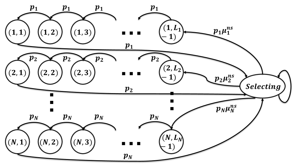
Figure 9: State Transfer Diagram for networks employing NSRPssource $i$

Suppose that the system state is $Selecting$ at time slot $t$, there are two categories of scheduling decisions can be made:

• Selecting Source $i$ with probability $\mu^{ns}_{i}$, i.e. $u_{i}(t)=1$, then the waiting time is given by

  $$W_{i}=\begin{cases}1,&\text{with probability }p_{i},\\ 1+W_{i},&\text{with probability }1-p_{i},\end{cases}$$ (79)

• Selecting Source $j\neq i$ with probability $\mu^{ns}_{j}$, i.e. $u_{j}(t)=1$, then the waiting time is given by

  $$W_{i}=Y_{j}+W_{i}$$ (80)

  $$Y_{j}=\begin{cases}1,&\text{with probability }1-p_{j},\\ 1+S_{j},&\text{with probability }p_{j},\end{cases}$$ (81)

  where each $S_{j}$ is service time of source $j$, and the total time spent include and after selecting source $j$ is $Y_{j}$, after which the BS returns to $Selecting$.

Next, we calculate the first moment $\mathbb{E}[W_{i}]$ and the second moment $\mathbb{E}[W^{2}_{i}]$ of the waiting time, respectively. We split the first moment $\mathbb{E}[W_{i}]$ conditional on the scheduling decision as

$$\mathbb{E}[W_{i}]=\mu^{ns}_{i}\mathbb{E}[W_{i}\mid u_{i}(t)=1]+\sum_{j\neq i}\mu^{ns}_{j}\mathbb{E}[W_{i}\mid u_{j}(t)=1].$$ (82)

where the conditional expectation are given by

$$\mathbb{E}[W_{i}\mid u_{i}(t)=1]=p_{i}\cdot 1+(1-p_{i})(1+\mathbb{E}[W_{i}])=1+(1-p_{i})\mathbb{E}[W_{i}].$$ (83)

$$\mathbb{E}[W_{i}\mid u_{j}(t)=1]=\mathbb{E}[Y_{j}]+\mathbb{E}[W_{i}].$$ (84)

Taking the expectation of total time spent after selecting source $Y_{j}i$ and substituting with (77) yields

$$\mathbb{E}[Y_{j}]=(1-p_{j})\cdot 1+p_{j}\left(1+\mathbb{E}[S_{j}]\right)=L_{j}.$$ (85)

Substituting (85) into (84) yields

$$\mathbb{E}[W_{i}\mid u_{j}(t)=1]=L_{i}+\mathbb{E}[W_{i}].$$ (86)

Thus, substituting (83) and  (86) into (82) yields

$$\mathbb{E}[W_{i}]=\frac{\mu^{ns}_{i}+\sum_{j\neq i}\mu^{ns}_{j}L_{j}}{\mu^{ns}_{i}p_{i}}.$$ (87)

Similarly, we condition on the scheduling decision to write

$$E[W_{i}^{2}]=\mu^{ns}_{i}\,\mathbb{E}[W_{i}^{2}\mid u_{i}(t)=1]+\sum_{j\neq i}\mu^{ns}_{j}\,\mathbb{E}[W_{i}^{2}\mid u_{j}(t)=1].$$ (88)

And the expectation conditional on source $i$ is selected is given by

$$\mathbb{E}[W_{i}^{2}\mid u_{i}(t)=1]=p_{i}\cdot 1^{2}+(1-p_{i})\mathbb{E}[(1+W_{i})^{2}],$$ (89)

Expanding the square yields

$$\mathbb{E}[W_{i}^{2}\mid u_{i}(t)=1]=p_{i}+(1-p_{i})\Bigl{(}1+2\mathbb{E}[W_{i}]+\mathbb{E}[W_{i}^{2}]\Bigr{)}=1+2(1-p_{i})\mathbb{E}[W_{i}]+(1-p_{i})\mathbb{E}[W_{i}^{2}].$$ (90)

Here, the waiting time for source $i$ is the sum of the time $Y_{j}$ spent after selecting source $j$ and the subsequent waiting time. And the expectation conditional on source $j\neq i$ is selected is given by

$$E[W_{i}^{2}\mid u_{j}(t)=1]=E\Bigl{[}(Y_{j}+W_{i})^{2}\Bigr{]}=\mathbb{E}[Y_{j}^{2}]+2\mathbb{E}[Y_{j}]\mathbb{E}[W_{i}]+\mathbb{E}[W_{i}^{2}].$$ (91)

Substituting (90) and (91)into (88) gives

$$\mathbb{E}[W_{i}^{2}] =\mu^{ns}_{i}\Bigl{[}1+2(1-p_{i})\mathbb{E}[W_{i}]+(1-p_{i})\mathbb{E}[W_{i}^{2}]\Bigr{]}$$

$$+\sum_{j\neq i}\mu^{ns}_{j}\Bigl{[}\mathbb{E}[Y_{j}^{2}]+2\mathbb{E}[Y_{j}]\mathbb{E}[W_{i}]+\mathbb{E}[W_{i}^{2}]\Bigr{]}.$$ (92)

Collecting the terms involving $\mathbb{E}[W_{i}^{2}]$ leads to

$$\mathbb{E}[W_{i}^{2}]=\frac{\mu^{ns}_{i}\Bigl{[}1+2(1-p_{i})\mathbb{E}[W_{i}]\Bigr{]}+\sum_{j\neq i}\mu^{ns}_{j}\Bigl{[}\mathbb{E}[Y_{j}^{2}]+2\mathbb{E}[Y_{j}]\mathbb{E}[W_{i}]\Bigr{]}}{1-\sum_{j}\mu^{ns}_{j}+p_{i}\mu^{ns}_{i}}.$$ (93)

Where the $\mathbb{E}[Y_{j}^{2}]$ is given by

$$\mathbb{E}[Y_{i}^{2}]=(1-p_{i})\cdot 1^{2}+p_{i}\mathbb{E}[(1+S_{i})^{2}].$$ (94)

Substituting (77) and (78) into (94) yields

$$\mathbb{E}[Y_{i}^{2}]=1+2(L_{i}-1)+\frac{(L_{i}-1)(L_{i}-p_{i})}{p_{i}}.$$ (95)

Thus, we obtain a close-from expression of NSRPs by organizing (76), (77), (78), (87), (93), and (95).

$$\mathbb{E}[J^{ns}]=\frac{1}{N}\sum_{i=1}^{N}\alpha_{i}\Biggl{[}\frac{\mu^{ns}_{i}p_{i}}{\sum^{N}_{j=1}\mu^{ns}_{j}L_{j}}\Biggl{(}\frac{\mathbb{E}[W^{2}_{i}]+\mathbb{E}[S^{2}_{i}]}{2}+\left(\frac{L_{i}-1}{p_{i}}\right)^{2}+2\mathbb{E}[W^{2}_{i}]\left(\frac{L_{i}-1}{p_{i}}\right)\Biggl{)}+1\Biggr{]}.$$ (96)

Where

$$\mathbb{E}[S^{2}_{i}] =\frac{(L_{i}-1)(L_{i}-p_{i})}{p_{i}^{2}},$$ (97)

$$\mathbb{E}[W_{i}] =\frac{\sum^{N}_{j=1}\mu^{ns}_{j}L_{j}-\mu^{ns}_{i}(L_{i}-1)}{\mu^{ns}_{i}p_{i}}.$$ (98)

$$\mathbb{E}[W_{i}^{2}] =\frac{\mu^{ns}_{i}\Bigl{[}1+2(1-p_{i})\mathbb{E}[W_{i}]\Bigr{]}+\sum_{j\neq i}\mu^{ns}_{j}\Bigl{[}\mathbb{E}[Y_{j}^{2}]+2\mathbb{E}[Y_{j}]\mathbb{E}[W_{i}]\Bigr{]}}{1-\sum_{j}\mu^{ns}_{j}+p_{i}\mu^{ns}_{i}}.,$$ (99)

$$\mathbb{E}[Y_{i}^{2}] =2L_{i}-1+\frac{(L_{i}-1)(L_{i}-p_{i})}{p_{i}}.$$ (100)

∎

Appendix F Upper Bound for Lyapunov Drift

In this appendix, we obtain the expressions in (29)– (31), which represent an upper bound on the Lyapunov Drift. Consider the network state $\mathbb{S}(t):=\{h_{i}(t),z_{i}(t),L_{i}(t),x_{i}(t)\}_{i=1}^{N}$, the Lyapunov Function in (27) and the Lyapunov Drift $\Delta\left(\mathbb{S}(t)\right)$ in (28). Substituting (27) into (28), we get

$$\Delta \left(\mathbb{S}(t)\right)=\frac{V}{2}\mathbb{E}\left[\sum_{i=1}^{N}\left[x^{+}_{i}(t+1)\right]^{2}-\sum_{i=1}^{N}\left[x^{+}_{i}(t)\right]^{2}|\mathbb{S}(t)\right]$$ (101)

$$+\mathbb{E}\left[\sum_{i=1}^{N}\beta_{i}\left[h_{i}(t+1)-z_{i}(t+1)\right]^{2}-\sum_{i=1}^{N}\beta_{i}\left[h_{i}(t)-z_{i}(t)\right]^{2}|\mathbb{S}(t)\right]$$

$$+\mathbb{E}\left[\sum_{i=1}^{N}\gamma_{i}\left[z_{i}(t+1)+L_{i}(t+1)\right]^{2}-\sum_{i=1}^{N}\gamma_{i}\left[z_{i}(t)+L_{i}(t)\right]^{2}|\mathbb{S}(t)\right]$$

Recall that the evolution of $L_{i}(t)$, $z_{i}(t)$, and $h_{i}(t)$ are given by  (1),  (2) and (3), respectively. The evolution of $h_{i}(t)-z_{i}(t)$ and $z_{i}(t)+L_{i}(t)$ are given by

$$h_{i}(t+1)-z_{i}(t+1)=\begin{cases}h_{i}(t)-z_{i}(t)+1&\text{if }d_{i}(t)=0\text{ and }L_{i}(t)=L,\\ z_{i}(t)&\text{if }d_{i}(t)=1\text{ and }L_{i}(t)=1,\\ h_{i}(t)-z_{i}(t)&\text{otherwise.}\end{cases}$$ (102)

$$z_{i}(t+1)+L_{i}(t+1)=\begin{cases}z_{i}(t)+L_{i}(t),&\text{if }d_{i}(t)=1\text{ and }L_{i}(t)>1\\ &\text{ or }L_{i}(t)=L,\\ L_{i}+1,&\text{if }d_{i}(t)=1\text{ and }L_{i}(t)=1,\\ z_{i}(t)+L_{i}(t)+1,&\text{otherwise.}\end{cases}$$ (103)

Substitute (102) and (103) into (101), leverage the discuss of throughput debt in [13, Appendix A], and rearrange the terms, we obtain  (29)–(31).

Appendix G Proof of Theorem 9

Theorem 9. For any given network model with network parameters $\{N,\alpha_{i},p_{i},L_{i}\}$, by choosing the constant $\beta_{i}=\frac{\alpha_{i}}{q_{i}^{L_{B}}},\gamma_{i}=\frac{\alpha_{i}}{q_{i}^{L_{B}}\sqrt{p_{i}}}$ and $\bar{q}_{i}=q^{L_{B}}_{i}-\epsilon$, where $\epsilon\rightarrow 0$, the optimality ratio of Max-Weight policy is such that

$$\rho=6+\frac{\sqrt{\varPsi}}{NL_{B}}$$ (104)

where

$$\varPsi=\left(\sum_{i=1}^{N}\alpha_{i}\right)\left(\sum_{i=1}^{N}\frac{\alpha_{i}}{\sqrt{p_{i}}}\left[5\frac{L^{2}_{i}\sqrt{p_{i}}}{\bar{q}^{2}_{i}}-\frac{L_{i}}{\bar{q}_{i}}-\frac{L_{i}\sqrt{p_{i}}}{\bar{q}_{i}}+2\frac{L^{2}_{i}}{\bar{q}^{2}_{i}}+2\frac{L_{i}^{2}}{\bar{q}_{i}}\right]\right)$$ (105)

The expression for the Lyapunov drift  (29)– (31) is central to the analysis in this appendix and is rewritten below for convenience.

$$\Delta\left(\mathbb{S}(t)\right)\leq B(t)-\sum_{i=1}^{N}p_{i}\mathbb{E}\left[u_{i}(t)|\mathbb{S}(t)\right]C_{i}(t)$$

where

$$B(t)= \sum_{i=1}^{N}\beta_{i}\mathbb{I}_{L_{i}(t)=L}\left[2h_{i}(t)-1\right]$$

$$+ \sum_{i=1}^{N}\gamma_{i}\mathbb{I}_{L_{i}(t)>1}\left[2\left(z_{i}(t)+L_{i}(t)\right)-1\right]+V\left[x^{+}_{i}(t)\bar{q}_{i}+\frac{1}{2}\right],$$

$$C_{i}(t) =\beta_{i}\mathbb{I}_{L_{i}(t)=L}\left[2h_{i}(t)-1\right]+\beta_{i}\mathbb{I}_{L_{i}(t)=1}\left[h_{i}^{2}(t)-2h_{i}(t)z_{i}(t)\right]$$

$$+\gamma_{i}\mathbb{I}_{L_{i}(t)>1}\left[2z_{i}(t)+2L_{i}(t)-1\right]$$

$$+\gamma_{i}\mathbb{I}_{L_{i}(t)=1}\left[\left(z_{i}(t)+2\right)^{2}-\left(L_{i}+1\right)^{2}\right]+Vx^{+}(t).$$

Before we prove the upper bound of EWSAoI achieved by the Max-Weight policy, we first prove the lower bound for achievable throughput in the following Lemma 11.

Lemma 11.

The Max-Weight policy achieves any feasible set of minimum throughput targets $\{\bar{q}\}^{N}_{i=1}$, if there exists any SRP $s$ satisfies $p_{i}\mu^{s}_{i}\geq\bar{q},\forall i$.

Proof.

Summarizing (28) and take the average over the time-horizon yields

$$\frac{\mathbb{E}[\mathcal{L}(T+1)]}{T}-\frac{\mathbb{E}[\mathcal{L}(1)]}{T}\leq\frac{1}{T}\sum_{t=1}^{T}B(t)-\frac{1}{TN}\sum_{t=1}^{T}\sum_{i=1}^{N}p_{i}\mathbb{E}\left[u_{i}(t)|\mathbb{S}(t)\right]C_{i}(t),$$ (106)

and taking the limit as $T\to\infty$, we obtain

$$\frac{1}{N}\sum_{i=1}^{N}p_{i}\mathbb{E}\left[u_{i}(t)C_{i}(t)\right]\leq\mathbb{E}\left[B(t)\right]$$ (107)

Recall that the Max-Weight policy minimizes the RHS of (29) by selecting $i=arg\max{C_{i}(t)}$ in every slot $t$. Hence, any other policy $\pi\in\Pi$ yields a lower (or equal) RHS. Consider a SRP $s\in\Pi^{s}_{r}$ that, in each slot $t$, selects node $i$ with probability $\mu^{s}_{i}\in(0,1]$. The scheduling decision of policy $s$ is independent with network state, yields

$$\sum_{i=1}^{N}p_{i}\mathbb{E}\left[u_{i}(t)|\mathbb{S}(t)\right]C_{i}(t)\geq\sum_{i=1}^{N}p_{i}\mu_{i}^{s}C_{i}(t)$$ (108)

where $u^{S}_{i}(t)$ denote the scheduling decision made by optimal SRP $S$.

The furhter analysis yields

$$\frac{1}{T}\sum_{t=1}^{T}\sum_{i=1}^{N}p_{i}\mathbb{E}\left[u_{i}(t)|\mathbb{S}(t)\right]C_{i}(t)\geq\frac{1}{T}\sum_{t=1}^{T}\sum_{i=1}^{N}p_{i}\mathbb{E}\left[u^{S}_{i}(t)|\mathbb{S}(t)\right]C_{i}(t)$$ (109)

where both sides of (109) are the extended expectation, which can be simplified as

$$\sum_{i=1}^{N}p_{i}\mathbb{E}\left[u_{i}(t)C_{i}(t)\right]\geq\sum_{i=1}^{N}p_{i}\mu_{i}^{s}\mathbb{E}\left[C_{i}(t)\right]$$ (110)

Substitute (30) and (31) into (110) and rearrange the terms, we obtain (111) on the top of next page. For simplicity of exposition, we divide inequality (111) into six terms $LHS_{1}+LHS_{2}+LHS_{3}\leq RHS_{1}+RHS_{2}+RHS_{3}$, gives

$$\begin{gathered}\sum_{i=1}^{N}p_{i}\mu^{s}_{i}\mathbb{E}[\mathbb{I}_{L_{i}(t)=1}]\mathbb{E}\left[\beta_{i}\left(h^{2}_{i}(t)-2h_{i}(t)z_{i}(t)\right)+\gamma_{i}\left(\left(z_{i}(t)+2\right)^{2}-\left(L_{i}+1\right)^{2}\right)\mid L_{i}(t)=1\right]+\sum_{i=1}^{N}V\left(p_{i}\mu^{s}_{i}-q_{i}\right)x_{i}^{+}(t)\\ \leq\sum_{i=1}^{N}\beta_{i}\mathbb{E}[\mathbb{I}_{L_{i}(t)=L}]\mathbb{E}\left[2h_{i}(t)-1\mid L_{i}(t)=L\right]+\sum_{i=1}^{N}\gamma_{i}\mathbb{E}[\mathbb{I}_{L_{i}(t)>1}]\mathbb{E}\left[2z_{i}(t)+2L_{i}(t)-1\mid L_{i}(t)>1\right]+\frac{NV}{2}\end{gathered}$$ (111)

 

$$LHS_{1}=\sum_{i=1}^{N}p_{i}\mu^{s}_{i}\beta_{i}\mathbb{E}[\mathbb{I}_{L_{i}(t)=1}]\mathbb{E}\left[h^{2}_{i}(t)-2h_{i}(t)z_{i}(t)\mid L_{i}(t)=1\right]$$ (112)

$$LHS_{2}=\sum_{i=1}^{N}p_{i}\mu^{s}_{i}\gamma_{i}\mathbb{E}[\mathbb{I}_{L_{i}(t)=1}]\mathbb{E}\left[\left(z_{i}(t)+2\right)^{2}-\left(L_{i}+1\right)^{2}\mid L_{i}(t)=1\right]$$ (113)

$$LHS_{3}=\sum_{i=1}^{N}V\left(p_{i}\mu^{s}_{i}-q_{i}\right)\mathbb{E}[x_{i}^{+}(t)]$$ (114)

$$RHS_{1}=\sum_{i=1}^{N}\beta_{i}(1-p_{i}\mu_{i})\mathbb{E}[\mathbb{I}_{L_{i}(t)=L}]\mathbb{E}\left[2h_{i}(t)-1\mid L_{i}(t)=L\right]$$ (115)

$$RHS_{2}=\sum_{i=1}^{N}\gamma_{i}(1-p_{i}\mu_{i})\mathbb{E}[\mathbb{I}_{L_{i}(t)>1}]\mathbb{E}\left[2z_{i}(t)+2L_{i}(t)-1\mid L_{i}(t)>1\right]$$ (116)

$$RHS_{3}=\frac{NV}{2}$$ (117)

Since that $LHS_{1}>-\infty$, $LHS_{2},RHS_{1}>,RHS_{2},RHS_{3}$ are positive, we establish that

$$\lim_{T\rightarrow}\frac{1}{T}\sum_{t=1}^{T}\mathbb{E}[x_{i}^{+}(t)]<\infty,$$ (118)

which is sufficient to establish that the throughput achieved by Max-Weight policy satisfies that $q_{i}^{MW}\geq\bar{q}_{i},\forall i$. [26, Theorem 2.8] ∎

Next, we leverage Lemma 11 to prove the upper bound for EWSAoI associate with Max-Weight policy in Theorem 9.

Consider a set of target throughput subject to

$$\bar{q}_{i}=q_{i}^{L_{B}}-\sigma,\quad\forall i,$$ (119)

where $\sigma\rightarrow 0$. By setting $\{\bar{q}_{i}\}_{i=1}^{N}$ as the target value in the throughput debt $x^{+}_{i}(t)$, since there exists a SRP $\mu_{i}^{L_{B}}=q_{i}^{L_{B}}/p_{i}$, the throughput achieve by Max-Weight policy, i.e. $\{q^{MW}_{i}\}_{i=1}^{N}$, satisfies

$$q^{MW}_{i}\geq q_{i}^{L_{B}}-\sigma,\quad\forall i.$$ (120)

Substitute (31) into (107), notice that $q^{MW}_{i}=p_{i}\mathbb{E}\left[u_{i}(t)\right]$ we obtain $LHS^{\prime}_{1}+LHS^{\prime}_{2}+LHS^{\prime}_{3}\leq RHS^{\prime}_{1}+RHS^{\prime}_{2}+RHS^{\prime}_{3}$, which are given by

$$LHS^{\prime}_{1}= \sum_{i=1}^{N}q^{MW}_{i}\beta_{i}\mathbb{E}\left[\mathbb{I}_{L_{i}(t)=1}|u_{i}(t)=1\right]$$ (121)

$$\times\mathbb{E}\left[h^{2}_{i}(t)-2h_{i}(t)z_{i}(t)|u_{i}(t)=1,L_{i}(t)=1\right]$$

$$LHS^{\prime}_{2}= \sum_{i=1}^{N}q^{MW}_{i}\gamma_{i}\mathbb{E}\left[\mathbb{I}_{L_{i}(t)=1}|u_{i}(t)=1\right]$$ (122)

$$\times\mathbb{E}\left[\left(z_{i}(t)+2\right)^{2}-\left(L_{i}+1\right)^{2}|u_{i}(t)=1,L_{i}(t)=1\right]$$

$$LHS^{\prime}_{3}=\sum_{i=1}^{N}V\left(q^{MW}_{i}-\bar{q}_{i}\right)\mathbb{E}[x_{i}^{+}(t)]$$ (123)

$$RHS^{\prime}_{1}=\sum_{i=1}^{N}\beta_{i}\mathbb{E}[\mathbb{I}_{L_{i}(t)=L}]\mathbb{E}\left[2h_{i}(t)-1\mid L_{i}(t)=L\right]$$ (124)

$$RHS^{\prime}_{2}=\sum_{i=1}^{N}\gamma_{i}\mathbb{E}[\mathbb{I}_{L_{i}(t)>1}]\mathbb{E}\left[2z_{i}(t)+2L_{i}(t)-1\mid L_{i}(t)>1\right]$$ (125)

$$RHS^{\prime}_{3}=\frac{NV}{2}$$ (126)

Next, we analysis the packet transmission process and the bound for each term to simplify (121) – (126).

Notice that the sufficient and necessary condition for a update delivery of source $i$ is that $d_{i}(t)\mathbb{I}_{L_{i}(t)=1}=1$, and the time average update delivery of source $i$ is $\frac{q_{i}}{L_{i}}$, then we establish

$$\frac{q_{i}}{L_{i}}=\mathbb{E}[d_{i}(t)\mathbb{I}_{L_{i}(t)=1}]$$ (127)

Expending the expectation on the RHS yields

$$\mathbb{E}[d_{i}(t)\mathbb{I}_{L_{i}(t)=1}] =p_{i}\mathbb{E}\left[u_{i}(t)\mathbb{E}[\mathbb{I}_{L_{i}(t)=1}|u_{i}(t)]\right]$$ (128)

$$=p_{i}\mathbb{P}\left[u_{i}(t)=1\right]\mathbb{E}[\mathbb{I}_{L_{i}(t)=1}|u_{i}(t)=1]$$

Notice that $q_{i}=p_{i}\mathbb{P}\left[u_{i}(t)=1\right]$, further substituting (127) into (128) yields

$$\mathbb{E}[\mathbb{I}_{L_{i}(t)=1}|u_{i}(t)=1]=\frac{1}{L_{i}}$$ (129)

Recall that Max-Weight policy selects the source with the highest value of $C_{i}(t)$ at each given time slot. Thus we establish

$$\mathbb{E}\left[C_{i}(t)|u_{i}(t)=1\right]\geq\mathbb{E}\left[C_{i}(t)\right]$$ (130)

$$\mathbb{E}\left[C_{i}(t)|u_{i}(t)=1,L_{i}(t)=1\right]\geq\mathbb{E}\left[C_{i}(t)|L_{i}(t)=1\right]$$ (131)

Due to the sequential packets transmission, during each update delivery process, the value $h_{i}(t)-z_{i}(t)$ and $z_{i}(t)+L_{i}(t)$ is nondecreasing until the delivery of last packet, regardless of the channel and scheduling decision, so we establish

$$\mathbb{E}\left[C_{i}(t)|u_{i}(t)=1,L_{i}(t)=1\right]\geq\mathbb{E}\left[C_{i}(t)|u_{i}(t)=1\right]$$ (132)

Similarly, we obtain

$$\mathbb{E}\left[2h_{i}(t)-1\mid L_{i}(t)=L\right]\leq\mathbb{E}\left[2h_{i}(t)-1\right]$$ (133)

$$\mathbb{E}\left[2z_{i}(t)+2L_{i}(t)-1\mid L_{i}(t)>1\right]\leq\mathbb{E}\left[2z_{i}(t)+2L_{i}(t)-1\right]$$ (134)

Substitute (129), (132) and (130) into (121) and (122), we obtain

$$\begin{array}[]{ll}LHS^{\prime}_{1}+LHS^{\prime}_{2}&\stackrel{{\scriptstyle(a)}}{{\geq}}\sum_{i=1}^{N}\frac{q^{MW}_{i}\beta_{i}}{L_{i}}\mathbb{E}\left[h^{2}_{i}(t)-2h_{i}(t)z_{i}(t)\right]+\sum_{i=1}^{N}\frac{q_{i}^{MW}\gamma_{i}}{L_{i}}\mathbb{E}\left[\left(z_{i}(t)+2\right)^{2}-\left(L_{i}+1\right)^{2}|L_{i}(t)=1\right]\\ &\stackrel{{\scriptstyle(b)}}{{\geq}}\sum_{i=1}^{N}\frac{q^{MW}_{i}\beta_{i}}{L_{i}}\mathbb{E}\left[\left(h_{i}(t)-2z_{i}(t)\right)^{2}\right]+\sum_{i=1}^{N}\frac{q_{i}^{MW}\gamma_{i}}{L_{i}}\mathbb{E}\left[\left(z_{i}(t)+2\right)^{2}-\left(L_{i}+1\right)^{2}|L_{i}(t)=1\right]\\ &\stackrel{{\scriptstyle(c)}}{{\geq}}\sum_{i=1}^{N}\frac{q^{MW}_{i}\beta_{i}}{L_{i}}\left[\mathbb{E}\left[h_{i}(t)\right]-2\mathbb{E}\left[z_{i}(t)\right]\right]^{2}+\sum_{i=1}^{N}\frac{q_{i}^{MW}\gamma_{i}}{L_{i}}\left(\mathbb{E}\left[z_{i}(t)+2|L_{i}(t)=1\right]^{2}-\left(L_{i}+1\right)^{2}\right)\\ &\stackrel{{\scriptstyle(d)}}{{\geq}}\sum_{i=1}^{N}\frac{q^{MW}_{i}\beta_{i}}{L_{i}}\left[\mathbb{E}\left[h_{i}(t)\right]-2\mathbb{E}\left[z_{i}(t)\right]\right]^{2}\end{array}$$ (135)

where $(a)$ from (130), (131) and (132); $(b)$ from $h_{i}(t)>h_{i}(t)-2z_{i}(t)$; $(c)$ by applying Jensen Inequality $\mathbb{E}\left[\left(\bar{h}_{i}(t)-2z_{i}(t)\right)^{2}\right]\geq\left[\mathbb{E}\left[h_{i}(t)\right]-2\mathbb{E}\left[z_{i}(t)\right]\right]^{2}$, where $\bar{h}_{i}(t)=\max(h_{i}(t),2z_{i}(t))$ and $\mathbb{E}\left[\bar{h}_{i}(t)\right]\geq\mathbb{E}\left[h_{i}(t)\right]$; and $(d)$ from

$$\mathbb{E}\left[z_{i}(t)+2|L_{i}(t)=1\right]\geq L_{i}+1$$ (136)

Notice that $LHS^{\prime}_{2}+LHS^{\prime}_{3}>0,\mathbb{E}[\mathbb{I}_{L_{i}(t)=L}]<1,\mathbb{E}[\mathbb{I}_{L_{i}(t)>1}]<1$, substituting (133), (134) and (135) into $LHS^{\prime}_{1}+LHS^{\prime}_{2}+LHS^{\prime}_{3}\leq RHS^{\prime}_{1}+RHS^{\prime}_{2}+RHS^{\prime}_{3}$ yields

$$\sum_{i=1}^{N}\frac{q^{MW}_{i}\beta_{i}}{L_{i}}\left[\mathbb{E}\left[h_{i}(t)\right]-2\mathbb{E}\left[z_{i}(t)\right]\right]^{2}$$ (137)

$$\leq\sum_{i=1}^{N}\beta_{i}\mathbb{E}\left[2h_{i}(t)-1\right]+\sum_{i=1}^{N}\gamma_{i}\mathbb{E}\left[2z_{i}(t)+2L_{i}(t)-1\right]+\frac{NV}{2}$$

Substituting $\beta_{i}=\alpha_{i}L_{i}/\bar{q}_{i},\gamma_{i}=\alpha_{i}L_{i}/\bar{q}_{i}\sqrt{p_{i}}$ and considering $\sigma\rightarrow 0$ yields

$$\sum_{i=1}^{N}\alpha_{i}\left[\mathbb{E}\left[h_{i}(t)\right]-2\mathbb{E}\left[z_{i}(t)\right]\right]^{2}$$ (138)

$$\leq\sum_{i=1}^{N}\frac{\alpha_{i}L_{i}}{\bar{q}_{i}}\mathbb{E}\left[2h_{i}(t)-1\right]+\sum_{i=1}^{N}\frac{\alpha_{i}L_{i}}{\bar{q}_{i}\sqrt{p_{i}}}\mathbb{E}\left[2z_{i}(t)+2L_{i}(t)-1\right]+\frac{NV}{2}$$

Consider the Cauchy-Schwarz inequality

$$\left(\sum_{i=1}^{N}\alpha_{i}\left[\mathbb{E}\left[h_{i}(t)\right]-\frac{3L_{i}}{\bar{q}_{i}}\right]^{2}\right)\left(\sum_{i=1}^{N}\alpha_{i}\right)$$ (139)

$$\quad\geq\left|\sum_{i=1}^{N}\alpha_{i}\left[\mathbb{E}\left[h_{i}(t)\right]-\frac{3L_{i}}{\bar{q}_{i}}\right]\right|^{2}$$

Applying (139) and $\mathbb{E}\left[z_{i}(t)\right]\geq L_{i}/\bar{q}_{i}$ into (138) yields

$$\left(\sum_{i=1}^{N}\alpha_{i}\left[\mathbb{E}\left[h_{i}(t)\right]-\frac{3L_{i}}{\bar{q}_{i}}\right]^{2}\right)\left(\sum_{i=1}^{N}\alpha_{i}\right)$$ (140)

$$\leq\left(\sum_{i=1}^{N}\alpha_{i}\right)\left(\sum_{i=1}^{N}\frac{\alpha_{i}}{\sqrt{p_{i}}}\left[5\frac{L^{2}_{i}\sqrt{p_{i}}}{\bar{q}^{2}_{i}}-\frac{L_{i}}{\bar{q}_{i}}-\frac{L_{i}\sqrt{p_{i}}}{\bar{q}_{i}}+2\frac{L^{2}_{i}}{\bar{q}^{2}_{i}}+2\frac{L_{i}^{2}}{\bar{q}_{i}}\right]\right)$$

Thus, we obtain the upper bound od achieved by Max-Weight policy, which is given by

$$\mathbb{E}\left[J^{MW}\right]\leq\frac{1}{N}\sum_{i=1}^{N}\frac{3\alpha_{i}L_{i}}{\bar{q}_{i}}+\frac{1}{N}\sqrt{\varPsi}$$ (141)

where

$$\varPsi=\left(\sum_{i=1}^{N}\alpha_{i}\right)\left(\sum_{i=1}^{N}\frac{\alpha_{i}}{\sqrt{p_{i}}}\left[5\frac{L^{2}_{i}\sqrt{p_{i}}}{\bar{q}^{2}_{i}}-\frac{L_{i}}{\bar{q}_{i}}-\frac{L_{i}\sqrt{p_{i}}}{\bar{q}_{i}}+2\frac{L^{2}_{i}}{\bar{q}^{2}_{i}}+2\frac{L_{i}^{2}}{\bar{q}_{i}}\right]\right)$$ (142)

Comparing (141) with (12) yields

$$\rho=6+\frac{\sqrt{\varPsi}}{NL_{B}}$$ (143)

where $\rho$ is the optimal ratio of Max-Weight policy.

References

- [1] S. Kaul et al., “Minimizing age of information in vehicular networks,” in IEEE SECON, 2011, pp. 350–358.
- [2] C. Guo et al., “Age of information, latency, and reliability in intelligent vehicular networks,” IEEE Network, vol. 37, no. 6, pp. 109–116, 2023.
- [3] H. Hu et al., “AoI-minimal trajectory planning and data collection in uav-assisted wireless powered IoT networks,” IEEE Internet of Things Journal, vol. 8, no. 2, pp. 1211–1223, 2021.
- [4] B. Choudhury et al., “AoI-minimizing scheduling in uav-relayed IoT networks,” in Proc. IEEE MASS, 2021, pp. 117–126.
- [5] V. Tripathi et al., “WiSwarm: Age-of-information-based wireless networking for collaborative teams of UAVs,” in Proc. IEEE INFOCOM, 2023, pp. 1–10.
- [6] B. Yu, X. Chen, and Y. Cai, “Age of information for the cellular internet of things: Challenges, key techniques, and future trends,” IEEE Communications Magazine, vol. 60, no. 12, pp. 20–26, 2022.
- [7] H. B. Beytur et al., “Towards AoI-aware smart IoT systems,” in Proc. IEEE ICNC, 2020, pp. 353–357.
- [8] M. A. Abd-Elmagid et al., “On the role of age of information in the internet of things,” IEEE Communications Magazine, vol. 57, no. 12, pp. 72–77, 2019.
- [9] I. Kadota and E. Modiano, “Minimizing the age of information in wireless networks with stochastic arrivals,” IEEE Transactions on Mobile Computing, vol. 20, no. 3, pp. 1173–1185, 2019.
- [10] A. Zakeri et al., “Minimizing the AoI in resource-constrained multi-source relaying systems: Dynamic and learning-based scheduling,” IEEE Transactions on Wireless Communications, vol. 23, no. 1, pp. 450–466, 2023.
- [11] B. Zhou and W. Saad, “Joint status sampling and updating for minimizing age of information in the internet of things,” IEEE Transactions on Communications, vol. 67, no. 11, pp. 7468–7482, 2019.
- [12] H. Tang et al., “Minimizing age of information with power constraints: Multi-user opportunistic scheduling in multi-state time-varying channels,” IEEE Journal on Selected Areas in Communications, vol. 38, no. 5, pp. 854–868, 2020.
- [13] I. Kadota, A. Sinha, and E. Modiano, “Scheduling algorithms for optimizing age of information in wireless networks with throughput constraints,” IEEE/ACM Transactions on Networking, vol. 27, no. 4, pp. 1359–1372, 2019.
- [14] E. Fountoulakis et al., “Scheduling policies for AoI minimization with timely throughput constraints,” IEEE Transactions on Communications, vol. 71, no. 7, pp. 3905–3917, 2023.
- [15] E. U. Atay, I. Kadota, and E. Modiano, “Aging wireless bandits: Regret analysis and order-optimal learning algorithm,” in Proc. WiOpt, 2021.
- [16] J. Liu, Q. Wang, and H. Chen, “Optimizing information freshness in uplink multiuser mimo networks with partial observations,” arXiv preprint arXiv:2401.02218, 2024.
- [17] Z. Zhao and I. Kadota, “Optimizing age of information without knowing the age of information,” in Proc. IEEE INFOCOM, 2025.
- [18] I. Kadota et al., “Scheduling policies for minimizing age of information in broadcast wireless networks,” IEEE/ACM Transactions on Networking, vol. 26, no. 6, pp. 2637–2650, 2018.
- [19] C. Li et al., “Minimizing age of information under general models for iot data collection,” IEEE Transactions on Network Science and Engineering, vol. 7, no. 4, pp. 2256–2270, 2019.
- [20] V. Tripathi et al., “Computation and communication co-design for real-time monitoring and control in multi-agent systems,” in Proc. WiOpt, 2021.
- [21] B. Zhou and W. Saad, “Minimum age of information in the internet of things with non-uniform status packet sizes,” IEEE Transactions on Wireless Communications, vol. 19, no. 3, pp. 1933–1947, 2019.
- [22] C. Li et al., “Minimizing AoI in a 5G-based IoT network under varying channel conditions,” IEEE Internet of Things Journal, vol. 8, no. 19, pp. 14 543–14 558, 2021.
- [23] S. M. Ross, Introduction to probability models. Academic press, 2014.
- [24] M. Neely, Stochastic network optimization with application to communication and queueing systems. Springer Nature, 2022.
- [25] I.-H. Hou, V. Borkar, and P. R. Kumar, “A theory of QoS for wireless,” in Proc. IEEE INFOCOM, 2009.
- [26] M. J. Neely, “Stability and capacity regions or discrete time queueing networks,” arXiv preprint arXiv:1003.3396, 2010.
- [27] R. G. Gallager, Stochastic processes: theory for applications. Cambridge University Press, 2013.