Bayesian Inference for a Time-Fractional HIV Model with Nonlinear Diffusion

Abstract

This study investigates an inverse problem associated with a time-fractional HIV infection model incorporating nonlinear diffusion. The model describes the dynamics of uninfected target cells, infected cells, and free virus particles, where the diffusion terms are nonlinear density functions. The primary objective is to recover the unknown diffusion functions by utilizing final-time measurement data. Due to the inherent ill-posedness of the inverse problem and the presence of measurement noise, we employ a Bayesian inference framework to obtain stable and reliable estimates while quantifying uncertainty. To solve the inverse problem efficiently, we develop an Iterative Regularizing Ensemble Kalman Method (IREKM), which enables the simultaneous estimation of multiple diffusion terms without requiring gradient information. Numerical experiments validate the effectiveness of the proposed method in reconstructing the unknown diffusion terms under different noise levels, demonstrating its robustness and accuracy. These findings contribute to a deeper understanding of HIV infection dynamics and provide a computational approach for parameter estimation in fractional diffusion models.

Keywords: HIV model, time-fractional derivative, Nonlinear density function, Inverse problem, Bayesian inference; ensemble Kalman method

AMS Subject Classifications: 26A33, 35R11, 35R30, 62F15, 92D25

1 Introduction

In this paper, we study an inverse problem for the following time-fractional HIV infection model:

$$\displaystyle\left\{\begin{array}[]{l}\partial_{t}^{\alpha}u_{1}-\text{div}(D_{1}(u_{1})\nabla u_{1})=-du_{1}-\beta(u_{1},u_{3})-\sigma(u_{1},u_{2}),(x,t)\in\Omega_{T},\\ \partial_{t}^{\alpha}u_{2}-\text{div}(D_{2}(u_{2})\nabla u_{2})=\beta(u_{1},u_{3})+\sigma(u_{1},u_{2})-ru_{2},\quad(x,t)\in\Omega_{T},\\ \partial_{t}^{\alpha}u_{3}-\text{div}(D_{3}(u_{3})\nabla u_{3})=Nu_{2}-eu_{3},\qquad\qquad\qquad\qquad(x,t)\in\Omega_{T},\\ u_{1}(x,t)=u_{2}(x,t)=u_{3}(x,t)=0,\leavevmode\nobreak\ \qquad\qquad\qquad\qquad\qquad(x,t)\in\Gamma_{T},\\ u_{1}(x,0)=u_{1,0}(x),u_{2}(x,0)=u_{2,0}(x),u_{3}(x,0)=u_{3,0}(x),\qquad x\in\Omega,\end{array}\right.$$ (1.6)

where $\displaystyle\partial_{t}^{\alpha}$ is the Caputo fractional derivative of order $\displaystyle 0<\alpha<1$, $\displaystyle\Omega\subset\mathbb{R}^{n}$ is a bounded domain with a boundary $\displaystyle\partial\Omega$, $\displaystyle T>0$ is a final time, $\displaystyle\Omega_{T}=\Omega\times(0,T)$, $\displaystyle\Gamma_{T}=\partial\Omega\times(0,T)$, $\displaystyle u_{1}$ is the concentration of healthy cells, $\displaystyle u_{2}$ is the concentration of infected cells, $\displaystyle u_{3}$ is the concentration of healthy cells virions, $\displaystyle D_{1}(u_{1}),D_{2}(u_{2})$ and $\displaystyle D_{3}(u_{3})$ are the nonlinear density functions for $\displaystyle u_{1},u_{2}$ and $\displaystyle u_{3}$ respectively, $\displaystyle d=d(x,t)>0$ is the death rate for healthy cells, $\displaystyle N=N(x,t)>0$ is the virus production rate, $\displaystyle e=e(x,t)>0$ is the death rate of virions, $\displaystyle r=r(x,t)>0$ is the death rate of infected cells, $\displaystyle\beta(u_{1},u_{3})=\beta_{1}\,\frac{u_{1}u_{3}}{1+u_{1}}$, $\displaystyle\sigma(u_{1},u_{2})=\beta_{2}\,\frac{u_{1}u_{2}}{1+u_{1}}$, $\displaystyle\beta_{1}=\beta_{1}(x,t)>0$ is the virus infection rate, $\displaystyle\beta_{2}=\beta_{2}(x,t)>0$ is the cell-cell infection rate. We assume that $\displaystyle u_{1,0}(x),u_{2,0}(x)$ and $\displaystyle u_{3,0}(x)$ are in $\displaystyle L_{2}(\Omega)$, the set of square-integrable functions in $\displaystyle\Omega$ and $\displaystyle d(x,t),\beta_{1}(x,t),\beta_{2}(x,t),r(x,t),N(x,t),e(x,t)$ are in $\displaystyle C(\Omega_{T})$, the set of continuous functions on $\displaystyle\Omega_{T}$. For the given inputs $\displaystyle\alpha$, $\displaystyle T$, $\displaystyle D_{1}(u_{1}),D_{2}(u_{2}),D_{3}(u_{3})$, $\displaystyle d$, $\displaystyle\beta$, $\displaystyle\sigma$, $\displaystyle r$, $\displaystyle e$, $\displaystyle N$, $\displaystyle u_{1,0}$, $\displaystyle u_{2,0}$, $\displaystyle u_{3,0}$, the problem (1.6) is called the direct problem.

HIV (human immunodeficiency virus) attacks immune cells, impairing the body’s ability to combat infections and making individuals more susceptible to opportunistic diseases. If left untreated, HIV can progress to AIDS (acquired immunodeficiency syndrome). In recent years, several mathematical models have been developed to describe the dynamics of HIV infection and to analyze epidemic patterns associated with AIDS. For instance, in [1], a reaction-diffusion within-host HIV model incorporating cell mobility, spatial heterogeneity, and cell-to-cell transmission is proposed. The authors investigate the well-posedness and global dynamics of the model and analyze the influence of spatial heterogeneity and diffusion properties on virion propagation through numerical simulations. In [2], the authors introduce a mathematical model to examine the interaction between drug addiction and the spread of HIV/AIDS in Iranian prisons, studying the stability of the system. A separate study [3] formulates an ordinary differential equation model describing the dynamics of HIV/AIDS, focusing on control strategies and determining optimal conditions for disease management. Furthermore, [4] presents a preliminary analysis of HIV transmission dynamics, leveraging quantitative epidemiological data and simple deterministic models to describe viral spread and persistence. In [5], a mathematical model of HIV/AIDS transmission through sexual contact is proposed, incorporating asymptomatic and symptomatic phases as a system of differential equations. An epidemic model with multiple stages of infection and its global stability is analyzed in [6]. Another study [7] proposes an HIV dynamics model under distinct HAART (highly active antiretroviral therapy) regimens, predicting disease progression across all infection stages. However, fractional differential equations offer significant advantages over integer-order models in capturing the behavior of dynamical systems (see [8] - [17] and references therein). Based on this premise, the authors in [18] modified the model from [1] to study HIV spread and transmission dynamics within the host. The modifications include introducing time-fractional derivatives, density-dependent diffusion operators, and Holling type II functional responses to better capture HIV infection mechanisms within healthy cells. It is more realistic to consider density-dependent diffusion rather than linear diffusion in biological models, as the movement of infected cells through normal tissue resembles diffusion in a porous medium. Consequently, the random motility of infected cells is best represented as a function of the system’s state variables.

Recently, there has been growing interest in inverse problems involving fractional derivatives. In most of these studies, a fractional time derivative is considered, and the inverse problem typically involves determining this derivative, a source term, or a coefficient under some additional conditions. These problems are of significant physical and practical importance. However, the majority of existing research focuses on linear models (see [19] - [31] and the references therein). Inverse problems for nonlinear and nonlocal models constitute a relatively new area of study, with only a limited number of experimental investigations and analytical results. For instance, in [32], a nonlinear time-fractional inverse coefficient problem is examined, where the unknown coefficient depends on the gradient of the solution. The authors prove the existence of a unique solution to the direct problem and establish the existence of a quasi-solution for the inverse problem within the class of admissible coefficients. A similar problem, in which the unknown coefficient depends on the solution itself, is studied in [33]. In [34], the authors analyze numerical solutions for both the direct and inverse problems of a nonlinear, nonlocal time-fractional equation. They propose a numerical method based on discretizing the minimization problem and employing the steepest descent method alongside a least-squares approach to solve the inverse problem. The direct and inverse problems for a nonlinear time-fractional diffusion equation are investigated in [35], where a quasi-Newton optimization method is applied to obtain the numerical solution of the inverse problem. To address the ill-posedness of the inverse problem, Tikhonov regularization is utilized. In [36], an iterative method of lines scheme is developed for the numerical solution of the time-fractional Richards equation with implicit Neumann boundary conditions. Additionally, [37] examines an inverse problem for an inhomogeneous time-fractional diffusion equation in a one-dimensional real-positive semiaxis domain. The authors demonstrate that the inverse problem is severely ill-posed and apply a modified regularization method based on frequency-domain solutions to address this issue. In the present study, we investigate an inverse problem for the direct problem (1.6). Unlike the aforementioned studies, we consider a nonlinear and nonlocal system with nonlinear functions on the side, where three unknown nonlinear density functions must be simultaneously determined as part of the inverse problem. This approach represents a novel contribution to the field of inverse problems. Our study can be regarded as a continuation of the series of works on fractional inverse problems discussed above.

This paper is organized as follows: In the next section, we introduce the direct and inverse problems, providing the necessary mathematical background and formulation. Section 3 presents the Bayesian inference framework and the Iterative Regularizing Ensemble Kalman Method (IREKM) used for solving the inverse problem. Section 4 details numerical experiments that validate the proposed approach, including discussions on reconstruction accuracy, noise sensitivity, and computational performance. Finally, Section 5 provides concluding remarks, summarizing key findings and potential directions for future research.

2 The direct and the inverse problems

As mentioned in the Section 1, the fractional-time derivative $\displaystyle\partial_{t}^{\alpha}$ considered in (1.6) is the Caputo fractional derivative of order $\displaystyle 0<\alpha<1$ and is defined by

$$\displaystyle\partial_{t}^{\alpha}u(x,t):=\frac{1}{\Gamma(1-\alpha)}\int_{0}^{t}{(t-\xi)^{-\alpha}}\frac{\partial u(x,\xi)}{\partial\xi}d\xi,$$ (2.1)

where $\displaystyle\Gamma$ is the Gamma function. Kilbas et al [38] and Podlubny [39] can be referred for properties of the Caputo fractional derivative.

Definition 2.1.

[18] A set $\displaystyle\mathbb{D}$ satisfying the following conditions is called the class of admissible coefficients :

1. The Carathéodory functions $\displaystyle D_{i}(s):\Omega_{T}\times\mathbb{R}^{n}\to\mathbb{R},i=1,2,3$, are continuous functions with respect to $\displaystyle s$.

2. $\displaystyle|D_{i}(s)\xi|\leq\gamma_{i}\big{[}\wedge_{i}(x,t)+|\xi|\big{]}$, $\displaystyle\gamma_{i}>0$, $\displaystyle\xi\in\mathbb{R}^{n}$, $\displaystyle\wedge_{i}(x,t)\in L_{2}(\Omega_{T})$, $\displaystyle i=1,2,3$.

3. $\displaystyle\big{(}D_{i}(s)\xi-D_{i}(\hat{s})\hat{\xi}\big{)}\big{(}\xi-\hat{\xi}\big{)}\geq 0$, $\displaystyle\xi,\hat{\xi}\in\mathbb{R}^{n}$, $\displaystyle i=1,2,3$.

4. $\displaystyle|D_{i}(s)\xi|.\,\xi\geq b_{i}|\xi|^{2}$, $\displaystyle i=1,2,3$.

5. $\displaystyle D_{i}^{\prime}(s)\leq L$, $\displaystyle L>0,i=1,2,3$.

The conditions (ii) - (iv) are called Leray - Lions assumptions and arise in the solvability of the direct problem (1.6), see [18], [35], [36], [40]. Next, we define a weak solution to the direct problem (1.6).

Definition 2.2.

[18], A triplet of the functions $\displaystyle(u_{1},u_{2},u_{3})$ is called a weak solution to the direct problem (1.6) if $\displaystyle u_{1},u_{2},u_{3}\in L^{2}\left(0,T;H_{0}^{1}(\Omega)\right)\cap W_{2}^{\alpha}\left(0,T;L^{2}(\Omega)\right)$ such that the following integral identities hold for a.e. $\displaystyle t\in[0,T]$:

$$\displaystyle\left\{\begin{array}[]{l}\int\limits_{\Omega}\partial_{t}^{\alpha}u_{1}\,\varphi_{1}\,dx+\int\limits_{\Omega}D_{1}\left(u_{1}\right)\nabla u_{1}\cdot\nabla\varphi_{1}\,dx=-\int\limits_{\Omega}d\,u_{1}\,\varphi_{1}\,dx-\int\limits_{\Omega}\beta(u_{1},u_{3})\,\varphi_{1}\,dx-\int\limits_{\Omega}\sigma(u_{1},u_{2})\,\varphi_{1}\,dx,\\ \int\limits_{\Omega}\partial_{t}^{\alpha}u_{2}\,\varphi_{2}\,dx+\int\limits_{\Omega}D_{2}\left(u_{2}\right)\nabla u_{2}\cdot\nabla\varphi_{2}\,dx=\int\limits_{\Omega}\beta(u_{1},u_{3})\,\varphi_{2}\,dx+\int\limits_{\Omega}\sigma(u_{1},u_{2})\,\varphi_{2}\,dx-\int\limits_{\Omega}r\,u_{2}\,\varphi_{2}\,dx,\\ \int\limits_{\Omega}\partial_{t}^{\alpha}u_{3}\,\varphi_{3}\,dx+\int\limits_{\Omega}D_{3}\left(u_{3}\right)\nabla u_{3}\cdot\nabla\varphi_{3}\,dx=\int\limits_{\Omega}N\,u_{2}\varphi_{3}\,dx-\int\limits_{\Omega}e\,u_{3}\varphi_{3}\,dx,\end{array}\right.$$ (2.5)

for each $\displaystyle\varphi_{i}\in L^{2}\left(0,T;H_{0}^{1}(\Omega)\right)\,\cap\,W_{2}^{\alpha}\left(0,T;L_{2}(\Omega)\right)$, i = 1, 2, 3, where

$$W_{2}^{\alpha}(0,T):=\bigg{\{}u\in L^{2}[0,T]:\partial_{t}^{\alpha}u\in L^{2}[0,T]\,\bigg{\}}$$

is the fractional Sobolev space of order $\displaystyle\alpha$. Here we regard $\displaystyle u_{i}(x,t)$ as a mapping from $\displaystyle t\in(0,T)$ to $\displaystyle L^{2}(\Omega)$ and write $\displaystyle u_{i}(t)=u_{i}(\cdot,t)$.

In [18], it is proved that the direct problem (1.6) has a unique and non-negative weak solution. Now we prove the following theorem:

Theorem 2.1.

Let $\displaystyle D_{i},i=1,2,3\in\mathbb{D}$ and $\displaystyle(u_{1},u_{2},u_{3})\in L^{2}\left(0,T;H_{0}^{1}(\Omega)\right)\cap W_{2}^{\beta}\left(0,T;L^{2}(\Omega)\right)^{3}$ be the unique weak solution to the direct problem (1.6). Then the following estimates holds:

$$\partial_{t}^{\alpha}\bigg{(}\|u_{1}\|^{2}+\|u_{2}\|^{2}+\|u_{3}\|^{2}\bigg{)}+c\,\bigg{(}\|u_{1}\|_{H_{0}^{1}(\Omega)}^{2}+\|u_{2}\|_{H_{0}^{1}(\Omega)}^{2}+\|u_{3}\|_{H_{0}^{1}(\Omega)}^{2}\bigg{)}\,\leq C.$$ (2.6)

Proof.

By taking $\displaystyle\varphi_{1}=u_{1}$, $\displaystyle\varphi_{2}=u_{2}$ and $\displaystyle\varphi_{3}=u_{3}$ in (2.5), we have

$$\displaystyle\left\{\begin{array}[]{l}\int\limits_{\Omega}\partial_{t}^{\alpha}u_{1}\,u_{1}\,dx+\int\limits_{\Omega}D_{1}\left(u_{1}\right)|\nabla u_{1}|^{2}\,dx=-\int\limits_{\Omega}d\,u_{1}^{2}\,dx-\int\limits_{\Omega}\beta(u_{1},u_{3})\,u_{1}\,dx-\int\limits_{\Omega}\sigma(u_{1},u_{2})\,u_{1}\,dx,\\ \int\limits_{\Omega}\partial_{t}^{\alpha}u_{2}\,u_{2}\,dx+\int\limits_{\Omega}D_{2}\left(u_{2}\right)|\nabla u_{2}|^{2}\,dx=\int\limits_{\Omega}\beta(u_{1},u_{3})\,u_{2}\,dx+\int\limits_{\Omega}\sigma(u_{1},u_{2})\,u_{2}\,dx-\int\limits_{\Omega}r\,u_{2}^{2}\,dx,\\ \int\limits_{\Omega}\partial_{t}^{\alpha}u_{3}\,u_{3}\,dx+\int\limits_{\Omega}D_{3}\left(u_{3}\right)|\nabla u_{3}|^{2}\,dx=\int\limits_{\Omega}N\,u_{2}u_{3}\,dx-\int\limits_{\Omega}e\,u_{3}^{2}\,dx.\end{array}\right.$$ (2.10)

We evaluate the first integral identity in (2.10) as follows

$$\displaystyle\begin{split}\frac{1}{2}\partial_{t}^{\alpha}\|u_{1}\|^{2}+b_{1}&\|\nabla u_{1}\|^{2}\overset{\text{Alikhanov ineq. and (iv)}}{\leq}\int\limits_{\Omega}\partial_{t}^{\alpha}u_{1}\,u_{1}\,dx+\int\limits_{\Omega}D_{1}\left(u_{1}\right)|\nabla u_{1}|^{2}\,dx\\ &\qquad\qquad\qquad\quad=\int\limits_{\Omega}d\,u_{1}^{2}\,dx-\int\limits_{\Omega}\beta(u_{1},u_{3})\,u_{1}\,dx-\int\limits_{\Omega}\sigma(u_{1},u_{2})\,u_{1}\,dx\\ &\qquad\qquad\quad\overset{\text{Young's ineq.}}{\leq}C_{1}\bigg{(}\|u_{1}\|^{2}+\|u_{2}\|^{2}+\|u_{3}\|^{2}\bigg{)},\end{split}$$ (2.11)

where we used that $\displaystyle\beta(u_{1},u_{3})\leq\beta_{1}(x,t)u_{3}$, $\displaystyle\sigma(u_{1},u_{2})\leq\beta_{2}(x,t)u_{2}$ and $\displaystyle\beta_{1}(x,t),\beta_{2}(x,t)$ are in $\displaystyle C(\Omega_{T})$. Then (2.11) implies that

$$\displaystyle\frac{1}{2}\partial_{t}^{\alpha}\|u_{1}\|^{2}+b_{1}\|\nabla u_{1}\|^{2}\leq C_{1}\bigg{(}\|u_{1}\|^{2}+\|u_{2}\|^{2}+\|u_{3}\|^{2}\bigg{)}.$$ (2.12)

Similarly we get that

$$\displaystyle\begin{split}&\frac{1}{2}\partial_{t}^{\alpha}\|u_{2}\|^{2}+b_{2}\|\nabla u_{2}\|^{2}\leq C_{2}\bigg{(}\|u_{2}\|^{2}+\|u_{3}\|^{2}\bigg{)},\\ &\frac{1}{2}\partial_{t}^{\alpha}\|u_{3}\|^{2}+b_{3}\|\nabla u_{3}\|^{2}\leq C_{3}\bigg{(}\|u_{2}\|^{2}+\|u_{3}\|^{2}\bigg{)}.\end{split}$$ (2.13)

Finally, combining (2.12) and (2.13) together, we deduce that

$$\displaystyle\frac{1}{2}\partial_{t}^{\alpha}\bigg{(}\|u_{1}\|^{2}+\|u_{2}\|^{2}+\|u_{3}\|^{2}\bigg{)}+b\bigg{(}\|\nabla u_{1}\|^{2}+\|\nabla u_{2}\|^{2}+\|\nabla u_{3}\|^{2}\bigg{)}\leq c\bigg{(}\|u_{1}\|^{2}+\|u_{2}\|^{2}+\|u_{3}\|^{2}\bigg{)}.$$ (2.14)

By Lemma 2.4 in [41], we obtain the proof. ∎

Theorem 2.2.

Suppose that a sequence of coefficients $\displaystyle\{D_{i,n}\}\in\mathbb{D}$ converges pointwise in $\displaystyle[0,\infty)$ to a function $\displaystyle D_{i}(u)\in\mathbb{D},i=1,2,3$. Then the sequence of solutions $\displaystyle u_{i,n}:=u(x,t;D_{i,n})$ converges to the solution $\displaystyle u_{i}:=u(x,t;D_{i})\in L^{2}\left(0,T;H_{0}^{1}(\Omega)\right)\cap W_{2}^{\beta}\left(0,T;L^{2}(\Omega)\right)$, for $\displaystyle i=1,2,3.$

Proof.

The proof can be derived by closely following Lemma 4 in [18]. ∎

In this paper we study an inverse problem that consists of determining the functions $\displaystyle(U(x,t),D(x,t))$, where $\displaystyle U(x,t)=(u_{1}(x,t),u_{2}(x,t),u_{3}(x,t))$ and $\displaystyle D(u)=\big{(}D_{1}(u),D_{2}(u),D_{3}(u)\big{)}$, from the following final time measured data:

$$u_{i}(x,T)=\psi_{i}(x),i=1,2,3,(x,t)\in\Omega.$$ (2.15)

For the consistency of the initial conditions in (1.6) and the measured data in (2.15), we assume that $\displaystyle\psi_{i}(x)=0,i=1,2,3,x\in\partial\Omega$. We denote by $\displaystyle U(x,t;D)$ the solution to the direct problem (1.6) for a given $\displaystyle D\in\mathbb{D}$ and set the following input-output mapping:

$$\mathbb{F}_{i}(D_{i}):D_{i}\longrightarrow u_{i}(x,T)=\psi_{i}(x),i=1,2,3,x\in\partial\Omega,$$ (2.16)

where $\displaystyle\mathbb{F}_{i}(D_{i}):\mathbb{D}\longrightarrow H_{0}^{1}(\Omega).$ By Theorem 2.2 , it is clear that input-output mapping is continuous. The following theorem is straightforward with Theorem 2.2 and Theorems 1.1 and 1.2 in [42].

Theorem 2.3.

If the prior $\displaystyle\mu_{0}$ is any measure with $\displaystyle\mu_{0}{(X)}=1$, then the Bayesian inverse problem of recovering $\displaystyle D(u)=\big{(}D_{1}(u),D_{2}(u),D_{3}(u)\big{)}$ from the data $\displaystyle d=\mathbb{F}(D)+\varepsilon$, $\displaystyle\varepsilon\thicksim\mathcal{N}(0,C)$, is well-defined and the solution in the Bayesian framework depends continuously on the data.

3 Bayesian framework

In this section, we present a numerical approach to identifying the diffusion terms $\displaystyle(D_{1},D_{2},D_{3})$ in the context of the HIV infection model (1.6). The available experimental data, denoted by $\displaystyle y$, is assumed to correspond to key biological quantities: the concentrations of uninfected target cells $\displaystyle u(x,t)$, infected cells $\displaystyle v(x,t)$, and the free virus particles $\displaystyle w(x,t)$, which are the solutions to the time-fractional HIV infection model. Specifically, the data points $\displaystyle y=(u(x,T),v(x,T),w(x,T))$ are measured at the final time $\displaystyle T$, representing the observed spatial distribution of these biological quantities. These measurements provide critical insights into the dynamics of HIV infection, enabling the estimation of the diffusion terms that govern the spatial spread of the infection within tissue. Accurate identification of these terms is essential for understanding disease progression and optimizing treatment strategies.

Our objective is to estimate the diffusion terms $\displaystyle(D_{1},D_{2},D_{3})$ using the experimental data $\displaystyle y$. However, the presence of measurement noise introduces significant uncertainty into the estimation process, complicating the inverse problem. Additionally, the inherent ill-posedness of the problem further exacerbates these challenges, necessitating the use of regularization techniques to obtain stable and reliable solutions.

To account for uncertainties arising from both observational noise and prior knowledge, we adopt a Bayesian inference framework. This approach not only estimates the unknown parameter vector $\displaystyle D=(D_{1},D_{2},D_{3})$ but also quantifies the associated uncertainty by constructing the posterior probability distribution of the parameters. The theoretical foundations of this framework are well-established in the works of Chada et al. [43], Cotter et al. [44], Dashti et al. [45], Iglesias et al. [46, 47] , Kaipio et al. [48] and Stuart et al. [49]. Furthermore, the numerical aspects of Bayesian inverse problems have been extensively studied by Yan et al. [50] - [52].

To formalize the Bayesian framework, let us introduce $\displaystyle\varepsilon$ as Gaussian noise with mean of zero and the covariance matrix $\displaystyle C=\sigma^{2}I$, where $\displaystyle I$ is the identity matrix and $\displaystyle\sigma$ is the noise standard deviation. The noisy observation data $\displaystyle d$ can be expressed as:

$$d=\mathbb{F}(D)+\varepsilon,$$

where $\displaystyle\mathbb{F}(D)$ represents the observation operator, which is defined by the experimental data $\displaystyle y$.

In the Bayesian context, both $\displaystyle D$ and $\displaystyle d$ are treated as random variables, and the posterior distribution is given by Bayes’ theorem:

$$\mathbb{P}(D|d)\propto\mathbb{P}(d|D)\mathbb{P}(D),$$

where $\displaystyle\mathbb{P}(D)=\mathbb{P}(D_{1})\otimes\mathbb{P}(D_{2})\otimes\mathbb{P}(D_{3})$ is the prior distribution before the data is observed, with each $\displaystyle\mathbb{P}(D_{i})$ assumed to be Gaussian: $\displaystyle\mathbb{P}(D_{1})=\mathcal{N}(m_{1},C_{1})$, $\displaystyle\mathbb{P}(D_{2})=\mathcal{N}(m_{2},C_{2})$, and $\displaystyle\mathbb{P}(D_{3})=\mathcal{N}(m_{3},C_{3})$. The likelihood function $\displaystyle\mathbb{P}(d|D)$ is given by:

$$\mathbb{P}(d|D)\propto\exp\left(-\frac{1}{2}\|C^{-\frac{1}{2}}(d-\mathbb{F}(D))\|^{2}\right).$$

Once the posterior distribution is obtained, the next step is to extract meaningful information, typically by sampling from the posterior density. Markov Chain Monte Carlo (MCMC) methods are commonly used for this purpose, but they are computationally expensive, especially for large-scale problems. Although MCMC offers an exhaustive exploration of the posterior distribution, its high computational cost can limit its practical use. In such cases, ensemble-based methods provide an efficient alternative, capturing the essential characteristics of the posterior distribution with fewer evaluations of the forward model.

In this study, we extend the Iterative Regularizing Ensemble Kalman Method (IREKM), as introduced by Iglesias et al. [53] and Zhang et al. [54], to address the inverse problem of simultaneously determining the diffusion terms $\displaystyle D=(D_{1},D_{2},D_{3})$ in the time-fractional HIV infection model (1.6).

Algorithm 1 provides the pseudocode of the IREKM.

1. Generate the initial ensemble $\displaystyle\left\{D_{0}^{j}\right\}_{j=1}^{N_{e}}$ from the prior distribution $\displaystyle\mathbb{P}(D)$ of $\displaystyle D=(D_{1},D_{2},D_{3})$, where $\displaystyle N_{e}$ is the sample size. Let $\displaystyle d^{j}=d+\xi^{j}$, where $\displaystyle\xi^{j}\sim\mathcal{N}(0,C),j=1,2,3,\ldots,N_{e}$. Set $\displaystyle n=0.$

2. Let $\displaystyle D_{n}^{j}=(D_{1,n}^{j},D_{2,n}^{j},D_{3,n}^{j})$, $\displaystyle j=1,2,\dots,N_{e}.$ Calculate $\displaystyle z_{n}^{j}=\mathbb{F}(D_{n}^{j}),\quad\text{for}\quad j\in\{1,2,\ldots,N_{e}\},$ and compute the ensemble mean

   $$\overline{z}_{n}=\frac{1}{N_{e}}\sum_{j=1}^{N_{e}}z_{n}^{j}.$$

   Let

   $$\displaystyle C_{n}^{zz} \displaystyle=\frac{1}{N_{e}-1}\sum_{j=1}^{N_{e}}(\mathbb{F}(D_{n}^{j})-\overline{z}_{n})(\mathbb{F}(D_{n}^{j})-\overline{z}_{n})^{T},$$

   $$\displaystyle C_{n}^{D_{i}z} \displaystyle=\frac{1}{N_{e}-1}\sum_{j=1}^{N_{e}}(D_{i,n}^{j}-\overline{D}_{i,n})(\mathbb{F}(D_{n}^{j})-\overline{z}_{n})^{T},\text{ for }i=1,2,3.$$

   where

   $$\overline{D}_{i,n}=\frac{1}{N_{e}}\sum_{j=1}^{N_{e}}D_{i,n}.$$

3. Update each ensemble member

   $$D_{i,n+1}^{j}=D_{i,n}^{j}+C_{n}^{D_{i}z}(C_{n}^{zz}+\vartheta_{n}C)^{-1}(d^{j}-z_{n}^{j}),\quad j\in\{1,2,\ldots,N_{e}\},\,i\in\{1,2,3\},$$

   where $\displaystyle\vartheta_{n}$ is chosen as follows: Let $\displaystyle\vartheta_{0}$ be an initial guess, and $\displaystyle\vartheta_{n}^{i+1}=2^{i}\vartheta_{0}$. Choose $\displaystyle\vartheta_{n}=\vartheta_{n}^{M}$ where $\displaystyle M$ is the first integer such that

   $$\vartheta_{n}^{M}\|C^{-\frac{1}{2}}(C_{n}^{zz}+\vartheta_{n}^{M}C)^{-1}(d-\overline{z}_{n})\|\geq\mu\|C^{-1}(d-\overline{z}_{n})\|,$$

   and $\displaystyle\mu\in(0,1)$ is a constant.

4. Increase $\displaystyle n$ by one and go Step 2, repeat the above procedure until a stopping criterion is satisfied.

5. Take $\displaystyle\overline{D}_{n}=(\overline{D}_{1,n},\overline{D}_{2,n},\overline{D}_{3,n})$ as the numerical solution of $\displaystyle(D_{1},D_{2},D_{3})$.

Algorithm 1 Iterative Regularizing Ensemble Kalman Method (IREKM)

In Algorithm 1, we employ the Iterative Regularizing Ensemble Kalman Method (IREKM), a derivative-free optimization technique that effectively addresses the inverse problem of reconstructing the diffusion term in the HIV infection model. This method eliminates the need for computing adjoint problems, which are typically required in gradient-based optimization approaches. By bypassing the complexity of calculating gradients, particularly in cases where such computations are difficult or infeasible, IREKM provides a robust and efficient alternative for solving inverse problems in nonlinear models, such as those encountered in biological systems like HIV infection. Moreover, IREKM’s ability to simultaneously recover multiple parameters without relying on traditional alternating iteration methods further enhances its suitability for reconstructing the diffusion term in this context. For a deeper understanding of the numerical theory behind IREKM, readers are referred to detailed discussions in works such as [53, 56]. Schillings et al. [57] offers a convergence analysis for linear inverse problems, although the convergence of IREKM in nonlinear contexts remains an open research question, as highlighted by Iglesias et al. [53]. This paper focuses on the practical implementation of IREKM for the reconstruction of the diffusion term within the HIV infection model (1.6).

4 Numerical experiments

In this section, we present numerical experiments designed to validate the effectiveness of the proposed Bayesian inference framework for identifying the diffusion terms in the HIV infection model. These experiments demonstrate the capability of the Iterative Regularizing Ensemble Kalman Method (IREKM) to recover the parameters $\displaystyle(D_{1},D_{2},D_{3})$ from noisy observations, highlighting the robustness and accuracy. Through these simulations, we also examine the impact of different noise levels and prior information on the estimation process, providing valuable insights into the performance of the proposed approach.

4.1 Numerical solutions of the forward problem

In this section, we aim to address the direct problem (1.6) numerically. Specifically, we consider the direct problem (1.6) with the inclusion of source functions to facilitate the numerical approximation while maintaining the essential characteristics of the original problem.

$$\displaystyle\left\{\begin{array}[]{l}\partial_{t}^{\alpha}u_{1}-\text{div}(D_{1}(u_{1})\nabla u_{1})=-du_{1}-\beta(u_{1},u_{3})-\sigma(u_{1},u_{2})+f_{1}(x,t),(x,t)\in\Omega_{T},\\ \partial_{t}^{\alpha}u_{2}-\text{div}(D_{2}(u_{2})\nabla u_{2})=\beta(u_{1},u_{3})+\sigma(u_{1},u_{2})-ru_{2}+f_{2}(x,t),\quad(x,t)\in\Omega_{T},\\ \partial_{t}^{\alpha}u_{3}-\text{div}(D_{3}(u_{3})\nabla u_{3})=Nu_{2}-eu_{3}+f_{3}(x,t),\qquad\qquad\qquad\qquad(x,t)\in\Omega_{T},\\ u_{1}(x,t)=u_{2}(x,t)=u_{3}(x,t)=0,\leavevmode\nobreak\ \leavevmode\nobreak\ \qquad\qquad\qquad\qquad\qquad\qquad\qquad(x,t)\in\Gamma_{T},\\ u_{1}(x,0)=u_{1,0}(x),u_{2}(x,0)=u_{2,0}(x),u_{3}(x,0)=u_{3,0}(x),\qquad\qquad\qquad x\in\Omega.\end{array}\right.$$ (4.6)

In the following subsections, we outline our approach to numerically solving the coupled system. We start by describing the numerical techniques and methods used to approximate solutions to the system of equations. This includes an explanation of our discretization schemes and approximation strategies. In the second part, we perform rigorous tests and analyses to evaluate the accuracy and reliability of our numerical solutions. The validation process aims to confirm the robustness of our methodology in addressing the forward problem.

4.1.1 Approximation method

In this section, we explore the practical aspects of solving the forward problem within a numerical framework. Specifically, we employ the implicit-explicit finite difference scheme to approximate the behavior of the problem under consideration. Without loss of generality, we restrict our analysis to the one-dimensional case, where the spatial domain $\displaystyle\Omega$ is defined as $\displaystyle[a,b]$.

For the temporal approximation, we adopt the approach outlined in [58] - [60]. We divide the time interval $\displaystyle[0,T]$ into $\displaystyle M$ subintervals using equidistant nodal points:

$$t_{0}=0<t_{1}<\ldots<t_{M}=T,$$

with $\displaystyle t_{m}=mh_{t}$ for $\displaystyle m=0,\ldots,M$, where $\displaystyle h_{t}=T/M$ is the step length. Based on Y. Lin and C. Xu [58], we can approximate the Caputo fractional derivative in time using a simple quadrature formula as follows, for all $\displaystyle 0\leq m\leq M-1$:

$$\partial_{t}^{\alpha}\vartheta\left(x,t_{m+1}\right) =\frac{1}{\Gamma(1-\alpha)}\sum_{j=0}^{m}\int_{t_{j}}^{t_{j+1}}\frac{\partial_{s}\vartheta(x,s)}{\left(t_{m+1}-s\right)^{\alpha}}\,\mathrm{d}s$$

$$=\frac{1}{\Gamma(1-\alpha)}\sum_{j=0}^{m}\frac{\vartheta\left(x,t_{j+1}\right)-\vartheta\left(x,t_{j}\right)}{h_{t}}\int_{t_{j}}^{t_{j+1}}\frac{\mathrm{d}s}{\left(t_{m+1}-s\right)^{\alpha}}+r_{h_{t}}^{m+1}$$

$$=\frac{h_{t}^{-\alpha}}{\Gamma(2-\alpha)}\sum_{j=0}^{m}\big{[}\vartheta\left(x,t_{j+1}\right)-\vartheta\left(x,t_{j}\right)\big{]}\,\big{[}\left(m+1-j\right)^{1-\alpha}-\left(m-j\right)^{1-\alpha}\big{]}+r_{h_{t}}^{m+1}$$

$$=\frac{h_{t}^{-\alpha}}{\Gamma(2-\alpha)}\sum_{j=0}^{m}\big{[}\vartheta\left(x,t_{m+1-j}\right)-\vartheta\left(x,t_{m-j}\right)\big{]}\,\big{[}\left(j+1\right)^{1-\alpha}-j^{1-\alpha}\big{]}+r_{h_{t}}^{m+1},$$

where $\displaystyle r_{h_{t}}^{m+1}$ is the truncation error and satisfies $\displaystyle r_{h_{t}}^{m+1}\leq c\,h_{t}^{2-\alpha}$.

For the sake of simplification, let us introduce the notations $\displaystyle c_{\alpha}:=h_{t}^{\alpha}\,\Gamma(2-\alpha)$ and $\displaystyle b_{j}^{\alpha}:=\left(j+1\right)^{1-\alpha}-j^{1-\alpha}$, for $\displaystyle j=0,1,\dots,m$. We define the discrete fractional differential operator $\displaystyle\widetilde{\partial_{t}^{\alpha}}$ as:

$$\widetilde{\partial_{t}^{\alpha}}\vartheta\left(x,t_{m+1}\right):=\frac{1}{c_{\alpha}}\sum_{j=0}^{m}b_{j}^{\alpha}\,\big{[}\vartheta\left(x,t_{m+1-j}\right)-\vartheta\left(x,t_{m-j}\right)\big{]}.$$

It is straightforward to observe that $\displaystyle\widetilde{\partial_{t}^{\alpha}}\vartheta\left(x,t_{m+1}\right)$ can be rewritten as follows:

$$\widetilde{\partial_{t}^{\alpha}}\vartheta\left(x,t_{m+1}\right):=\frac{1}{c_{\alpha}}\vartheta\left(x,t_{m+1}\right)-\frac{1}{c_{\alpha}}\Phi^{m}(\vartheta),$$

where the term $\displaystyle\Phi^{m}(\vartheta)$ is defined as follows:

$$\Phi^{m}(\vartheta):=\left\{\begin{array}[]{ll}\vartheta\left(x,t_{m}\right),&\text{ if }m=0\\ \vartheta\left(x,t_{m}\right)-\sum_{j=1}^{m}b_{j}^{\alpha}\,\big{[}\vartheta\left(x,t_{m+1-j}\right)-\vartheta\left(x,t_{m-j}\right)\big{]},&\text{ if }1\leq m\leq M-1.\end{array}\right.$$

Hereafter, we denote by $\displaystyle\vartheta^{m}$ the approximated solution at the time $\displaystyle t_{m}$, for all $\displaystyle m=0,\dots,M$, i.e. $\displaystyle\vartheta^{m}=\vartheta(x,t_{m})$ for all $\displaystyle x\in\Omega$. Under these considerations, the time discretization of system (4.6) reads as follows:

$$\left\{\begin{array}[]{ll}\widetilde{\partial_{t}^{\alpha}}u_{1}^{m+1}-\operatorname{\text{div}}\left(D_{1}(u_{1}^{m})\nabla u_{1}^{m+1}\right)=-d^{m+1}u_{1}^{m+1}-\beta(u_{1}^{m},u_{3}^{m})-\sigma(u_{1}^{m},u_{2}^{m})+f_{1}^{m+1},&\text{ in }\Omega\\ \widetilde{\partial_{t}^{\alpha}}u_{2}^{m+1}-\operatorname{\text{div}}\left(D_{2}(u_{2}^{m})\nabla u_{2}^{m+1}\right)=\beta(u_{1}^{m},u_{3}^{m})+\sigma(u_{1}^{m},u_{2}^{m})-r^{m+1}u_{2}^{m+1}+f_{2}^{m+1},&\text{ in }\Omega\\ \widetilde{\partial_{t}^{\alpha}}u_{3}^{m+1}-\operatorname{\text{div}}\left(D_{3}(u_{3}^{m})\nabla u_{3}^{m+1}\right)=N^{m+1}u_{2}^{m}-e^{m+1}u_{3}^{m+1}+f_{3}^{m+1},&\text{ in }\Omega.\end{array}\right.$$ (4.7)

for all $\displaystyle 0\leq m\leq M-1$, with

$$u_{1}^{0}=u_{1,0}(x);\,u_{2}^{0}=u_{2,0}(x);\,u_{3}^{0}=u_{3,0}(x)\text{ in }\Omega$$

$$u_{1}^{m+1}=u_{2}^{m+1}=u_{3}^{m+1}=0\text{ on }\partial\Omega,\;\text{ for all }0\leq m\leq M-1.$$

Similarly, for discretizing the spatial domain, we introduce a set of evenly spaced grid points $\displaystyle\left(x_{i}\right){0\leq i\leq N}$ defined as $\displaystyle x_{i}=a+ih_{x}$, where $\displaystyle N$ is an integer, and the spacing $\displaystyle h_{x}$ is determined by $\displaystyle h_{x}=(b-a)/N$. At the boundaries of the domain $\displaystyle\Omega=[a,b]$, we have $\displaystyle x_{0}=a$ and $\displaystyle x_{N}=b$. For each pair $\displaystyle(x_{i},t_{m})$, with $\displaystyle 0\leq m\leq M$ and $\displaystyle 0\leq i\leq N$, we seek the numerical value of the solution, denoted as $\displaystyle\vartheta\left(x_{i},t_{m}\right)$. We enforce boundary and initial conditions such that $\displaystyle\vartheta\left(x_{0},t_{m}\right)=\vartheta\left(x_{N},t_{m}\right)=0$ for all $\displaystyle 0\leq m\leq M$ and $\displaystyle\vartheta\left(x_{i},t_{0}\right)=0$ for all $\displaystyle 0\leq i\leq N$. To approximate the spatial derivatives, we commonly employ central difference formulas due to their ability to provide enhanced accuracy. The differential equation is applied exclusively at the grid points, and the approximations for the first and second derivatives are as follows:

$$\begin{gathered}\partial_{x}\vartheta(x_{i},t_{m})\approx\frac{\vartheta(x_{i+1},t_{m})-\vartheta(x_{i-1},t_{m})}{2h_{x}},\\ \partial_{x}^{2}\vartheta(x_{i},t_{m})\approx\frac{\vartheta(x_{i+1},t_{m})-2\vartheta(x_{i},t_{m})+\vartheta(x_{i-1},t_{m})}{h_{x}^{2}}\end{gathered}$$

From now on, we denote by $\displaystyle u_{k,i}^{m}$ the discrete mesh function approximating $\displaystyle u_{k}(x_{i},t_{m})$ for $\displaystyle k=1,2,3$, $\displaystyle i=0,\dots,N$, and $\displaystyle m=0,\dots,M$. With this notation in place, we introduce a fully discrete scheme for the problem (4.6):

• Given

  $$u_{1,i}^{0}=u_{1,0}(x_{i}),\,\;u_{2,i}^{0}=u_{2,0}(x_{i}),\,\;u_{3,i}^{0}=u_{3,0}(x_{i}),\;\;\text{ for all }0\leq i\leq N,$$

  and

  $$u_{1,i}^{m+1}=u_{2,i}^{m+1}=u_{3,i}^{m+1}=0\text{ for all }0\leq m\leq M-1\;\text{ and }i\in\{0,N\}.$$

• Find the vector $\displaystyle\Lambda^{m+1}$, for all $\displaystyle 0\leq m\leq M-1$, which is defined as:

  $$\Lambda^{m+1}:=\left(u_{1,1}^{m+1},\dots,u_{1,N-1}^{m+1},u_{2,1}^{m+1},\dots,u_{2,N-1}^{m+1},u_{3,1}^{m+1},\dots,u_{3,N-1}^{m+1}\right)^{T}$$

  such that it satisfies the following linear system of equations

  $$\small\left\{\begin{array}[]{l}\frac{c_{\alpha}}{h_{x}^{2}}({}_{1}\mathbb{D}_{i}^{m}-\frac{{}_{1}\mathbb{D}_{i+1}^{m}-{}_{1}\mathbb{D}_{i-1}^{m}}{4})u_{1,i-1}^{m+1}+(1+\frac{2{}_{1}\mathbb{D}_{i}^{m}c_{\alpha}}{h_{x}^{2}}+c_{\alpha}d_{i}^{m+1})u_{1,i}^{m+1}-\frac{c_{\alpha}}{h_{x}^{2}}({}_{1}\mathbb{D}_{i}^{m}+\frac{{}_{1}\mathbb{D}_{i+1}^{m}-{}_{1}\mathbb{D}_{i-1}^{m}}{4})u_{1,i+1}^{m+1}={}_{1}\mathcal{F}_{i}^{m},\\ \\ \frac{c_{\alpha}}{h_{x}^{2}}({}_{2}\mathbb{D}_{i}^{m}-\frac{{}_{2}\mathbb{D}_{i+1}^{m}-{}_{2}\mathbb{D}_{i-1}^{m}}{4})u_{2,i-1}^{m+1}+(1+\frac{2{}_{2}\mathbb{D}_{i}^{m}c_{\alpha}}{h_{x}^{2}}+c_{\alpha}r_{i}^{m+1})u_{2,i}^{m+1}-\frac{c_{\alpha}}{h_{x}^{2}}({}_{2}\mathbb{D}_{i}^{m}+\frac{{}_{2}\mathbb{D}_{i+1}^{m}-{}_{2}\mathbb{D}_{i-1}^{m}}{4})u_{2,i+1}^{m+1}={}_{2}\mathcal{F}_{i}^{m},\\ \\ \frac{c_{\alpha}}{h_{x}^{2}}({}_{3}\mathbb{D}_{i}^{m}-\frac{{}_{3}\mathbb{D}_{i+1}^{m}-{}_{3}\mathbb{D}_{i-1}^{m}}{4})u_{3,i-1}^{m+1}+(1+\frac{2{}_{3}\mathbb{D}_{i}^{m}c_{\alpha}}{h_{x}^{2}}+c_{\alpha}e_{i}^{m+1})u_{3,i}^{m+1}-\frac{c_{\alpha}}{h_{x}^{2}}({}_{3}\mathbb{D}_{i}^{m}+\frac{{}_{3}\mathbb{D}_{i+1}^{m}-{}_{3}\mathbb{D}_{i-1}^{m}}{4})u_{3,i+1}^{m+1}={}_{3}\mathcal{F}_{i}^{m},\end{array}\right.$$ (4.8)

  where

  $$\left\{\begin{array}[]{l}{}_{1}\mathbb{D}(x,t)=D_{1}(u_{1}(x,t));\,{}_{2}\mathbb{D}(x,t)=D_{2}(u_{2}(x,t));\,{}_{3}\mathbb{D}(x,t)=D_{3}(u_{3}(x,t)),\,\,\text{ in }\Omega_{T},\\ \\ {}_{1}\mathcal{F}^{m}:=\Phi^{m}(u_{1})-c_{\alpha}\beta(u_{1}^{m},u_{3}^{m})-c_{\alpha}\sigma(u_{1}^{m},u_{2}^{m})+c_{\alpha}f_{1}^{m+1},\,\,\text{ in }\Omega,\\ \\ {}_{2}\mathcal{F}^{m}:=\Phi^{m}(u_{2})+c_{\alpha}\beta(u_{1}^{m},u_{3}^{m})+c_{\alpha}\sigma(u_{1}^{m},u_{2}^{m})+c_{\alpha}f_{2}^{m+1},\,\,\text{ in }\Omega,\\ \\ {}_{3}\mathcal{F}^{m}:=\Phi^{m}(u_{3})+c_{\alpha}N^{m+1}u_{2}^{m}+c_{\alpha}f_{3}^{m+1},\,\,\text{ in }\Omega.\end{array}\right.$$ (4.9)

Henceforth, it can be observed that this problem can be transformed into a matrix-based formulation to streamline its resolution. Specifically, we seek solutions to the system of equations:

$$\mathcal{A}\,\Lambda^{m+1}=\mathcal{F},\,\,\text{ for all }0\leq m\leq M-1,$$

where the matrix $\displaystyle\mathcal{A}$ and the right-hand side $\displaystyle\mathcal{F}$ are defined as follows:

$$\mathcal{A}=\left[\begin{array}[]{lll}U&0&0\\ 0&V&0\\ 0&0&W\end{array}\right]\;\;\text{ and }\;\;\mathcal{F}=\left[\begin{array}[]{c}{}_{1}F\\ {}_{2}F\\ {}_{3}F\end{array}\right].$$

Within this context, the tridiagonal matrices

$$U\in\mathcal{M}_{N-1}(\mathbb{R}),\;V\in\mathcal{M}_{N-1}(\mathbb{R}),\;\text{ and }W\in\mathcal{M}_{N-1}(\mathbb{R})$$

are defined for all $\displaystyle 1\leq p\leq N-1$ as follows:

$$U_{p-1,p}=\frac{c_{\alpha}}{h_{x}^{2}}\bigg{(}{}_{1}\mathbb{D}_{p}^{m}-\frac{{}_{1}\mathbb{D}_{p+1}^{m}-{}_{1}\mathbb{D}_{p-1}^{m}}{4}\bigg{)},\;U_{p,p}=1+\frac{2{}_{1}\mathbb{D}_{i}^{m}c_{\alpha}}{h_{x}^{2}}+c_{\alpha}d_{i}^{m+1},\;\text{ and }\,U_{p,p+1}=\frac{c_{\alpha}}{h_{x}^{2}}\bigg{(}{}_{1}\mathbb{D}_{p}^{m}+\frac{{}_{1}\mathbb{D}_{p+1}^{m}-{}_{1}\mathbb{D}_{p-1}^{m}}{4}\bigg{)},$$

$$V_{p-1,p}=\frac{c_{\alpha}}{h_{x}^{2}}\bigg{(}{}_{2}\mathbb{D}_{p}^{m}-\frac{{}_{2}\mathbb{D}_{p+1}^{m}-{}_{2}\mathbb{D}_{p-1}^{m}}{4}\bigg{)},\;V_{p,p}=1+\frac{2{}_{2}\mathbb{D}_{p}^{m}c_{\alpha}}{h_{x}^{2}}+c_{\alpha}r_{p}^{m+1},\;\text{ and }\,V_{p,p+1}=\frac{c_{\alpha}}{h_{x}^{2}}\bigg{(}{}_{2}\mathbb{D}_{p}^{m}+\frac{{}_{2}\mathbb{D}_{p+1}^{m}-{}_{2}\mathbb{D}_{p-1}^{m}}{4}\bigg{)},$$

$$W_{p-1,p}=\frac{c_{\alpha}}{h_{x}^{2}}\bigg{(}{}_{3}\mathbb{D}_{p}^{m}-\frac{{}_{3}\mathbb{D}_{p+1}^{m}-{}_{3}\mathbb{D}_{p-1}^{m}}{4}\bigg{)},\;W_{p,p}=1+\frac{2{}_{3}\mathbb{D}_{i}^{m}c_{\alpha}}{h_{x}^{2}}+c_{\alpha}e_{i}^{m+1},\;\text{ and }\,W_{p,p+1}=\frac{c_{\alpha}}{h_{x}^{2}}\bigg{(}{}_{3}\mathbb{D}_{p}^{m}+\frac{{}_{3}\mathbb{D}_{p+1}^{m}-{}_{3}\mathbb{D}_{p-1}^{m}}{4}\bigg{)},$$

respectively. Furthermore, the vectors

$${}_{1}F\in\mathbb{R}^{N-1},\;_{2}F\in\mathbb{R}^{N-1},\;\text{ and }\,_{3}F\in\mathbb{R}^{N-1}$$

are defined for all $\displaystyle 1\leq p\leq N-1$ as follows:

$${}_{1}F_{p}=_{1}\mathcal{F}_{p}^{m},\;_{2}F_{p}=_{2}\mathcal{F}_{p}^{m},\;\text{ and }\,_{3}F_{p}=_{3}\mathcal{F}_{p}^{m}.$$

To this end, the unknown term $\displaystyle\Lambda^{m+1}$, for $\displaystyle 0\leq m\leq M-1$, can be obtained as follows:

$$\Lambda^{m+1}=\mathcal{A}^{-1}\mathcal{F}.$$

4.1.2 Validation test

In this section, we conduct a validation test to assess the performance and accuracy of our numerical method. The objective is to compare the results obtained from our numerical approach with the exact solutions of the continuous model. To do so, we take the computational domain as $\displaystyle\Omega=[0,1]$ and set the final time as $\displaystyle T=1$. We consider three exact solutions as follows:

$$u_{1}^{\dagger}(x,t)=t^{\alpha}\sin(\pi x),\,\,u_{2}^{\dagger}(x,t)=tx^{2}(x-1),\,\text{ and }\,u_{3}^{\dagger}(x,t)=t^{2\alpha}x(1-x)\,\,\text{ for all }(x,t)\in\Omega_{T}.$$

It is evident that the exact solutions satisfy the following initial and boundary conditions:

$$u_{1}^{\dagger}(x,0)=u_{2}^{\dagger}(x,0)=u_{3}^{\dagger}(x,0)=0\text{ in }\Omega$$

$$u_{1}^{\dagger}(x,t)=u_{2}^{\dagger}(x,t)=u_{3}^{\dagger}(x,t)=0\text{ on }\Gamma_{T}.$$

The diffusion terms $\displaystyle D_{1}$, $\displaystyle D_{2}$, and $\displaystyle D_{3}$ are chosen as follows:

$$D_{1}(u_{1})=1+u_{1},\;\;D_{2}(u_{2})=(1+u_{2})^{2},\;\text{ and }\;D_{3}(u_{3})=1+u_{3}^{2}.$$

The functions $\displaystyle d$, $\displaystyle\beta_{1}$, $\displaystyle\beta_{2}$, $\displaystyle r$, $\displaystyle N$, and $\displaystyle e$ are given by:

$$d(x,t)=1+tx,\;\;\beta_{1}(x,t)=0.1,\;\;\beta_{2}(x,t)=0.01,\;\;r(x,t)=0.3,\;\;e(x,t)=0.001,\;\text{ and }\,N(x,t)=e^{xt}.$$

The source terms $\displaystyle f_{1}$, $\displaystyle f_{2}$, and $\displaystyle f_{3}$ can be computed by substituting this exact solutions into the system (4.6). To assess the accuracy of the proposed approximation method, we define the following error function:

$$\operatorname{\bf Err}_{k}(h_{t},h_{x}):=\|u_{k}^{\dagger}-\tilde{u}_{k}\|_{L^{\infty}(0,T;L_{2}(\Omega))},\quad\text{for }k=1,2,3.$$

Here, $\displaystyle\tilde{u}_{k}$ represents the approximated solution corresponding to the exact solution $\displaystyle u_{k}^{\dagger}$. The spatial and temporal convergence orders are computed by

$$\operatorname{\bf Ord}_{x}=\log_{2}\frac{\operatorname{\bf Err}_{k}(h_{t},h_{x})}{\operatorname{\bf Err}_{k}(h_{t},h_{x}/2)},\;\;\;\operatorname{\bf Ord}_{t}=\log_{2}\frac{\operatorname{\bf Err}_{k}(h_{t},h_{x})}{\operatorname{\bf Err}_{k}(h_{t}/2,h_{x})}.$$

In Table 1, we present the calculated error values in relation to the variation in the mesh size $\displaystyle h_{x}$, along with the corresponding convergence order $\displaystyle\operatorname{\bf Ord}_{x}$. This analysis is carried out for two values of $\displaystyle\alpha$, namely $\displaystyle\alpha=0.3$ and $\displaystyle\alpha=0.7$ while keeping the step time size $\displaystyle h_{t}$ fixed at $\displaystyle h_{t}=0.001$.

Derivative order $\displaystyle\alpha$	$\displaystyle h_{x}$	$\displaystyle\operatorname{\bf Err}_{1}$	$\displaystyle\operatorname{\bf Ord}_{x}$	$\displaystyle\operatorname{\bf Err}_{2}$	$\displaystyle\operatorname{\bf Ord}_{x}$	$\displaystyle\operatorname{\bf Err}_{3}$	$\displaystyle\operatorname{\bf Ord}_{x}$
$\displaystyle\alpha=0.3$	$\displaystyle 0.1$	$\displaystyle 1.97\text{\bf e-}2$	-	$\displaystyle 4.49\text{\bf e-}3$	-	$\displaystyle 6.53\text{\bf e-}4$	-
	$\displaystyle 0.05$	$\displaystyle 5.11\text{\bf e-}3$	$\displaystyle 1.9468$	$\displaystyle 1.02\text{\bf e-}3$	$\displaystyle 2.1381$	$\displaystyle 1.65\text{\bf e-}4$	$\displaystyle 1.9846$
	$\displaystyle 0.025$	$\displaystyle 1.21\text{\bf e-}3$	$\displaystyle 2.0783$	$\displaystyle 2.61\text{\bf e-}4$	$\displaystyle 1.9664$	$\displaystyle 4.23\text{\bf e-}5$	$\displaystyle 1.9637$
	$\displaystyle 0.0125$	$\displaystyle 3.33\text{\bf e-}4$	$\displaystyle 1.8614$	$\displaystyle 6.72\text{\bf e-}5$	$\displaystyle 1.9575$	$\displaystyle 1.04\text{\bf e-}5$	$\displaystyle 2.0240$
	$\displaystyle 0.00625$	$\displaystyle 7.45\text{\bf e-}5$	$\displaystyle 2.1602$	$\displaystyle 1.69\text{\bf e-}5$	$\displaystyle 1.9914$	$\displaystyle 2.74\text{\bf e-}6$	$\displaystyle 1.9243$
$\displaystyle\alpha=0.7$	$\displaystyle 0.1$	$\displaystyle 2.21\text{\bf e-}2$	-	$\displaystyle 4.77\text{\bf e-}3$	-	$\displaystyle 6.58\text{\bf e-}4$	-
	$\displaystyle 0.05$	$\displaystyle 5.31\text{\bf e-}3$	$\displaystyle 2.0572$	$\displaystyle 1.12\text{\bf e-}3$	$\displaystyle 2.0904$	$\displaystyle 1.71\text{\bf e-}4$	$\displaystyle 1.9440$
	$\displaystyle 0.025$	$\displaystyle 1.38\text{\bf e-}3$	$\displaystyle 1.9440$	$\displaystyle 2.70\text{\bf e-}4$	$\displaystyle 2.0524$	$\displaystyle 4.29\text{\bf e-}5$	$\displaystyle 1.9949$
	$\displaystyle 0.0125$	$\displaystyle 3.39\text{\bf e-}4$	$\displaystyle 2.0295$	$\displaystyle 6.80\text{\bf e-}5$	$\displaystyle 1.9893$	$\displaystyle 1.11\text{\bf e-}5$	$\displaystyle 1.9504$
	$\displaystyle 0.00625$	$\displaystyle 7.52\text{\bf e-}5$	$\displaystyle 2.1724$	$\displaystyle 1.81\text{\bf e-}5$	$\displaystyle 1.9095$	$\displaystyle 2.64\text{\bf e-}6$	$\displaystyle 2.0719$

Table 1: Convergence analysis for different mesh sizes $\displaystyle h_{x}$ and two values of $\displaystyle\alpha$ ($\displaystyle\alpha=0.3$ and $\displaystyle\alpha=0.7$) with a fixed step time size $\displaystyle h_{t}=0.001$.

In Table 2, we present the convergence analysis with respect to the step time size $\displaystyle h_{t}$ for $\displaystyle\alpha=0.3$ and $\displaystyle\alpha=0.7$ while keeping the mesh size fixed at $\displaystyle h_{x}=0.001$. The table provides the calculated error values and the corresponding convergence orders $\displaystyle\operatorname{\bf Ord}_{t}$ for different time step sizes.

Derivative order $\displaystyle\alpha$	$\displaystyle h_{t}$	$\displaystyle\mathrm{\bf Err}_{1}$	$\displaystyle\operatorname{\bf Ord}_{t}$	$\displaystyle\operatorname{\bf Err}_{2}$	$\displaystyle\operatorname{\bf Ord}_{t}$	$\displaystyle\operatorname{\bf Err}_{3}$	$\displaystyle\operatorname{\bf Ord}_{t}$
$\displaystyle\alpha=0.3$	$\displaystyle 0.1$	$\displaystyle 5.16\text{\bf e-}2$	-	$\displaystyle 1.38\text{\bf e-}3$	-	$\displaystyle 1.90\text{\bf e-}3$	-
	$\displaystyle 0.05$	$\displaystyle 2.73\text{\bf e-}2$	$\displaystyle 0.9184$	$\displaystyle 7.15\text{\bf e-}4$	$\displaystyle 0.9486$	$\displaystyle 9.75\text{\bf e-}4$	$\displaystyle 0.9625$
	$\displaystyle 0.025$	$\displaystyle 1.42\text{\bf e-}2$	$\displaystyle 0.9430$	$\displaystyle 3.68\text{\bf e-}4$	$\displaystyle 0.9582$	$\displaystyle 5.04\text{\bf e-}4$	$\displaystyle 0.9519$
	$\displaystyle 0.0125$	$\displaystyle 6.26\text{\bf e-}3$	$\displaystyle 1.1816$	$\displaystyle 1.75\text{\bf e-}4$	$\displaystyle 1.0723$	$\displaystyle 2.63\text{\bf e-}4$	$\displaystyle 0.9383$
	$\displaystyle 0.00625$	$\displaystyle 3.16\text{\bf e-}3$	$\displaystyle 0.9862$	$\displaystyle 8.11\text{\bf e-}5$	$\displaystyle 1.1095$	$\displaystyle 1.27\text{\bf e-}4$	$\displaystyle 1.0502$
$\displaystyle\alpha=0.7$	$\displaystyle 0.1$	$\displaystyle 1.05\text{\bf e-}2$	-	$\displaystyle 1.48\text{\bf e-}3$	-	$\displaystyle 2.41\text{\bf e-}3$	-
	$\displaystyle 0.05$	$\displaystyle 5.24\text{\bf e-}3$	$\displaystyle 1.0027$	$\displaystyle 7.47\text{\bf e-}4$	$\displaystyle 0.9864$	$\displaystyle 1.21\text{\bf e-}3$	$\displaystyle 0.9940$
	$\displaystyle 0.025$	$\displaystyle 2.32\text{\bf e-}3$	$\displaystyle 1.1754$	$\displaystyle 3.66\text{\bf e-}4$	$\displaystyle 1.0331$	$\displaystyle 6.16\text{\bf e-}4$	$\displaystyle 0.9740$
	$\displaystyle 0.0125$	$\displaystyle 1.12\text{\bf e-}3$	$\displaystyle 1.0506$	$\displaystyle 1.76\text{\bf e-}4$	$\displaystyle 1.0562$	$\displaystyle 3.18\text{\bf e-}4$	$\displaystyle 0.9539$
	$\displaystyle 0.00625$	$\displaystyle 5.72\text{\bf e-}4$	$\displaystyle 0.9694$	$\displaystyle 8.66\text{\bf e-}5$	$\displaystyle 1.0231$	$\displaystyle 1.49\text{\bf e-}4$	$\displaystyle 1.0937$

Table 2: Convergence analysis for different step time sizes $\displaystyle h_{t}$ and two values of $\displaystyle\alpha$ ($\displaystyle\alpha=0.3$ and $\displaystyle\alpha=0.7$) with a fixed mesh size $\displaystyle h_{x}=0.001$.

To this end, we illustrate in Figure 1 the variation of the exact and approximated solutions for $\displaystyle\alpha=0.5$ with $\displaystyle h_{x}=h_{t}=0.001.$

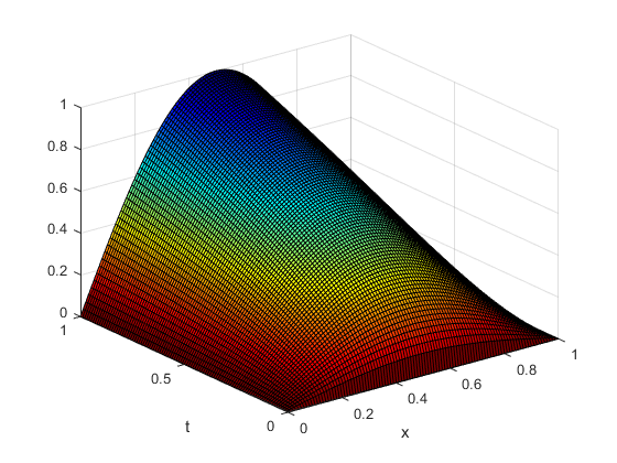
a Exact solution $\displaystyle u_{1}^{\dagger}$

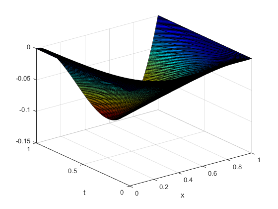
b Exact solution $\displaystyle u_{2}^{\dagger}$

c Exact solution $\displaystyle u_{3}^{\dagger}$

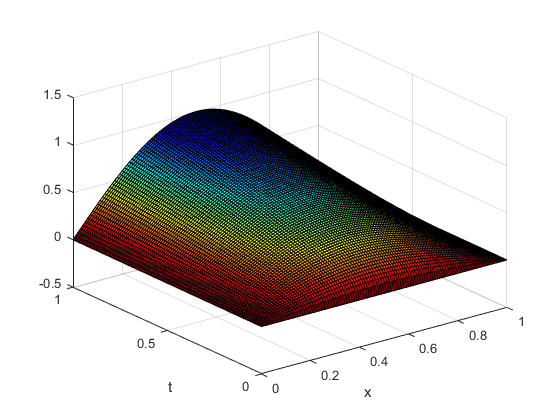
d Approximated solution $\displaystyle\tilde{u}_{1}$

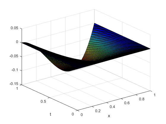
e Approximated solution $\displaystyle\tilde{u}_{2}$

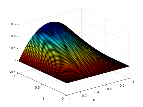
f Approximated solution $\displaystyle\tilde{u}_{3}$

Figure 1: Comparison of Exact and Approximated Solutions for $\displaystyle\alpha=0.5$ with $\displaystyle h_{x}=h_{t}=0.001$. The top row depicts the exact solutions, while the bottom row illustrates the approximated solutions.

4.2 Numerical solutions of the inverse problem

In this section, we present numerical results for three test cases to demonstrate the effectiveness of the Iterative Regularizing Ensemble Kalman Method (IREKM). Without loss of generality, we consider the computational domain $\displaystyle\Omega=(0,1)$ and the time horizon $\displaystyle T=1$. The direct problem (1.6) is solved using the proposed method described in the previous subsection. For the finite element algorithm, we discretize both the time and space domains with grid sizes $\displaystyle h_{t}=h_{x}=\frac{1}{100}$.

The source terms for the test cases are given by:

$$f_{1}(x,t)=f_{2}(x,t)=f_{3}(x,t)=0.$$

The initial conditions for the variables are:

$$u_{1,0}(x)=\sin(\pi x),\quad u_{2,0}(x)=x-x^{2},\quad u_{3,0}(x)=\sin(2\pi x).$$

To assess the accuracy of the numerical solution, we compute the approximate relative error, defined as

$$E_{n}=\frac{\left\|\overline{D}_{n}-D^{\dagger}\right\|_{2}}{\left\|D^{\dagger}\right\|_{2}},$$

where $\displaystyle\overline{D}_{n}=\left(\overline{D}_{1,n},\overline{D}_{2,n},\overline{D}_{3,n}\right)$ represents the mean values at the $\displaystyle n$th iteration of IREKM, and $\displaystyle D^{\dagger}=\left(D_{1}^{\dagger},D_{2}^{\dagger},D_{3}^{\dagger}\right)$ is the true solution of the inverse problem. The norm $\displaystyle\|\cdot\|_{2}$ denotes the Euclidean norm. Additionally, we monitor the residual $\displaystyle R_{n}$ at each iteration, given by

$$R_{n}=\left\|C^{-\frac{1}{2}}\left(d-\bar{z}_{n}\right)\right\|_{2}.$$

A crucial aspect of iterative algorithms is selecting an appropriate stopping criterion. Here, we employ the stopping rule proposed in [53, 46, 54], selecting $\displaystyle n_{\star}$ such that

$$R_{n_{\star}}\leq\tau\delta,$$

where $\displaystyle\tau>0$ is a constant, and $\displaystyle\delta=\left\|C^{-\frac{1}{2}}\left(d-\mathbb{F}\left(D^{\dagger}\right)\right)\right\|_{2}$ represents the noise level in the observed data.

In our numerical experiments, the prior distributions for $\displaystyle P(D_{1})$, $\displaystyle P(D_{2})$, and $\displaystyle P(D_{3})$ are chosen as

$$C_{i}=K_{i}A^{-s_{i}},\quad i=1,2,3,$$

where $\displaystyle A$ is the Laplace operator with homogeneous Dirichlet boundary conditions, and $\displaystyle s_{i}>\frac{1}{2}$ determines the regularity of the Gaussian prior. The initial mean values $\displaystyle\bar{D}_{i,0}$ for $\displaystyle i=1,2,3$ are taken as horizontal lines, with each line depending on the numerical example’s endpoint values. This choice is motivated by the fact that Bayesian inverse problems are highly sensitive to prior information selection. The key parameters used in the experiments are summarized in Table 3.

Parameter	$\displaystyle N_{e}$	$\displaystyle\vartheta_{0}$	$\displaystyle\nu$	$\displaystyle\tau$	$\displaystyle s_{1}$	$\displaystyle s_{2}$	$\displaystyle s_{3}$	$\displaystyle K_{1}$	$\displaystyle K_{2}$	$\displaystyle K_{3}$
Value	300	0.1	0.7	1.1	0.75	2	2	100	100	100

Table 3: Numerical values of the parameters used in the reconstruction process.

4.2.1 Reconstruction results

In the following, we present three test scenarios to validate the proposed reconstruction method for the diffusion terms in an HIV infection model. These scenarios feature different forms of diffusion for infected, healthy, and immune cells, each chosen to reflect various biological processes. The observed data for each test case are synthetic, generated to simulate realistic infection dynamics. It should be noted that all computations are performed using MATLAB version R2017a.

Example 1.

In this test, we apply the proposed algorithm to reconstruct the diffusion terms $\displaystyle D_{1}$, $\displaystyle D_{2}$, and $\displaystyle D_{3}$ in an HIV infection model, where the selection of these coefficients is biologically motivated by the distinct behaviors of infected, healthy, and immune cells. The diffusion of infected cells follows $\displaystyle D_{1}(u_{1})=1+0.5u_{1}$, indicating a linear dependence on their concentration.This means their spread increases proportionally as more cells become infected, representing a moderate yet steady propagation of infection. Healthy cells diffuse according to $\displaystyle D_{2}(u_{2})=1+0.3u_{2}^{2}$, where the quadratic dependence suggests an adaptive response to tissue damage, allowing faster regeneration as the healthy cell population grows. Immune cells follow $\displaystyle D_{3}(u_{3})=1+0.2u_{3}^{3}$, with a cubic dependence that captures an aggressive recruitment and activation mechanism, enhancing the immune response as more immune cells accumulate. These choices ensure that infected cells spread at a controlled rate, healthy cells migrate more efficiently as part of tissue repair, and immune cells exhibit a highly dynamic response to infection. This test case validates the reconstruction by employing the aforementioned diffusion terms, providing insight into how accurately they can be determined from observed data and assessing the spatial progression of infection and immune response.

The reconstruction results for $\displaystyle D_{1}(\cdot)$, $\displaystyle D_{2}(\cdot)$, and $\displaystyle D_{3}(\cdot)$ in Example 1 are illustrated in Figure 2 for the parameter value $\displaystyle\alpha=0.7$. These results provide insight into the accuracy and effectiveness of the proposed method in recovering the diffusion coefficients, highlighting how well the reconstructed profiles align with the expected behavior.

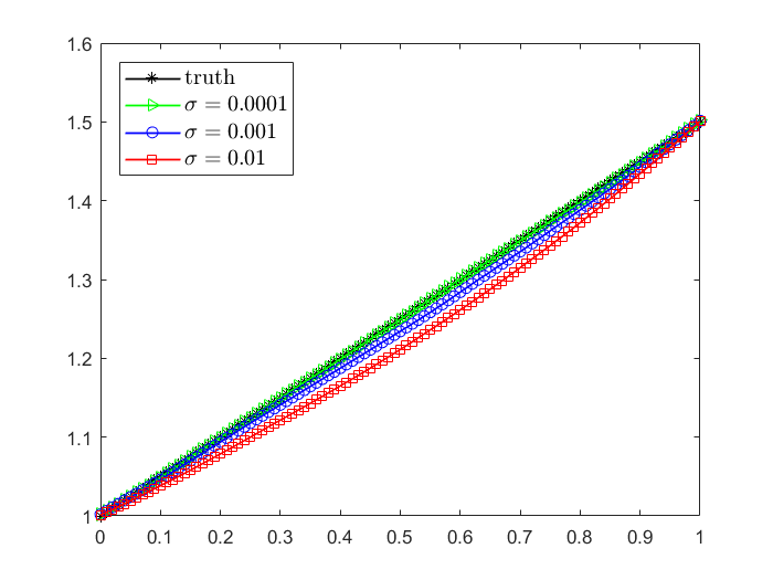
a

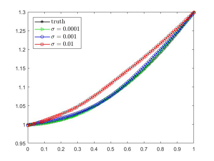
b

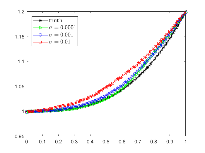
c

Figure 2: The numerical results of $\displaystyle D_{1}(\cdot)$ (left), $\displaystyle D_{2}(\cdot)$ (middle) and $\displaystyle D_{3}(\cdot)$ (right) for different noises $\displaystyle\sigma$ with $\displaystyle\alpha=0.7$ in Example 1.

Example 2.

Our objective is to reconstruct the diffusion coefficients $\displaystyle D_{1}$, $\displaystyle D_{2}$, and $\displaystyle D_{3}$ in an HIV infection model, where their selection is guided by biological reasoning. The diffusion of infected cells follows $\displaystyle D_{1}(u_{1})=\frac{1}{1+u_{1}^{2}}$, reflecting a saturation effect that restricts their movement at higher concentrations due to physical barriers or immune responses. Healthy cells diffuse according to $\displaystyle D_{2}(u_{2})=\frac{1}{1+u_{2}^{4}}$, modeling a scenario in which their mobility decreases as cell density increases, representing spatial competition during tissue repair. Immune cells, governed by $\displaystyle D_{3}(u_{3})=1+\frac{u_{3}}{1+u_{3}^{2}}$, exhibit a regulated diffusion pattern where their spread initially increases but slows at high concentrations, mimicking immune system limitations such as overcrowding or exhaustion. These diffusion models capture biologically relevant constraints, ensuring a more realistic representation of infection dynamics. This test case evaluates the feasibility of reconstructing these coefficients from the final time value observed data and provides insight into the interplay between infection spread, tissue recovery, and immune response.

Figure 3 shows the reconstruction results for $\displaystyle D_{1}(\cdot)$, $\displaystyle D_{2}(\cdot)$, and $\displaystyle D_{3}(\cdot)$ in Example 2 with the parameter value $\displaystyle\alpha=0.5$. These results highlight the method’s effectiveness in accurately recovering the diffusion coefficients, with the reconstructed profiles closely matching expected behavior.

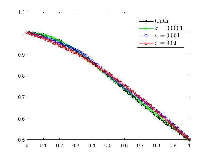
a

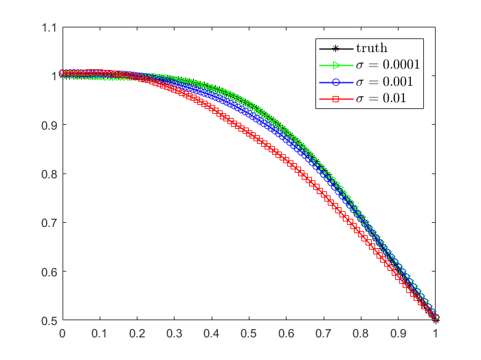
b

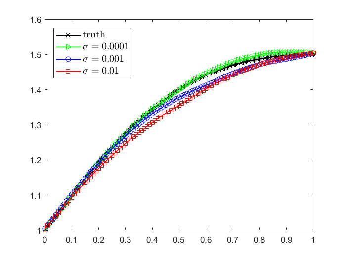
c

Figure 3: The numerical results of $\displaystyle D_{1}(\cdot)$ (left), $\displaystyle D_{2}(\cdot)$ (middle) and $\displaystyle D_{3}(\cdot)$ (right) for different noises $\displaystyle\sigma$ with $\displaystyle\alpha=0.5$ in Example 2.

Example 3.

In this test, we aim to reconstruct the diffusion terms $\displaystyle D_{1}$, $\displaystyle D_{2}$, and $\displaystyle D_{3}$ for an infection model with more complex and nonlinear forms of diffusion. The diffusion of infected cells is governed by $\displaystyle D_{1}(u_{1})=1+\sin(\pi u_{1})$, which introduces a sinusoidal variation in the diffusion, reflecting periodic fluctuations in the movement or interaction of infected cells. For healthy cells, the diffusion term is given by $\displaystyle D_{2}(u_{2})=\exp(u_{2}^{2}-u_{2})$, capturing an exponential growth and decay that may represent the tissue’s regenerative or deteriorative response to the presence of healthy cells. The diffusion term for immune cells follows $\displaystyle D_{3}(u_{3})=1+\exp(2u_{3})$, reflecting an exponential increase in diffusion as immune cells accumulate, which may correspond to enhanced immune response as the number of activated immune cells grows.

This test case is designed to assess the method’s ability to handle nonlinear, complex diffusion terms while providing valuable insight into the model’s adaptability to intricate biological processes. The reconstruction results for $\displaystyle D_{1}(\cdot)$, $\displaystyle D_{2}(\cdot)$, and $\displaystyle D_{3}(\cdot)$ in Example 3 are shown in Figure 4 for the parameter value $\displaystyle\alpha=0.2$. These results demonstrate the method’s capability to accurately recover the complex forms of the diffusion terms, illustrating how the reconstructed profiles align with expected behaviors of infection dynamics, tissue repair, and immune response.

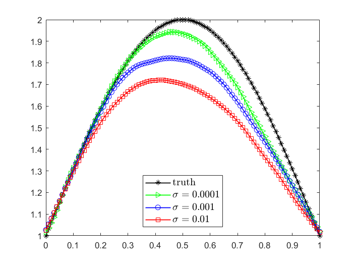
a

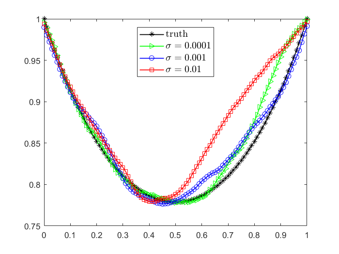
b

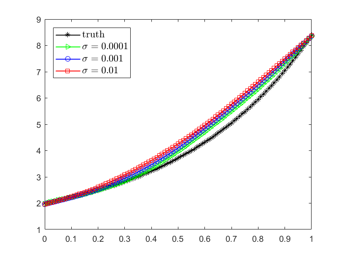
c

Figure 4: The numerical results of $\displaystyle D_{1}(\cdot)$ (left), $\displaystyle D_{2}(\cdot)$ (middle) and $\displaystyle D_{3}(\cdot)$ (right) for different noises $\displaystyle\sigma$ with $\displaystyle\alpha=0.2$ in Example 3.

4.2.2 Stability and convergence

The results presented in Figures 2, 3, and 4 demonstrate that reconstruction accuracy and precision improve as noise levels decrease. As noise is reduced, the numerical solution increasingly aligns with the true solution, highlighting the effectiveness of the method in achieving higher precision with cleaner data. This emphasizes IREKM’s sensitivity to noise and its ability to achieve greater accuracy in low-noise conditions. Furthermore, our approach successfully reconstructs various functional forms, including linear, quadratic, exponential, logistic, and sinusoidal behaviors. To further illustrate the stability and convergence of the proposed IREKM algorithm in addressing our inverse problem, Figure 5 depicts the logarithmic relative errors $\displaystyle\log_{10}(E_{n})$ and residuals $\displaystyle\log_{10}(R_{n})$ as functions of iteration count $\displaystyle n$ across different noise levels.

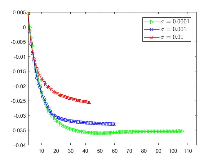
a

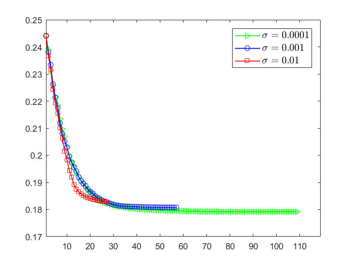
b

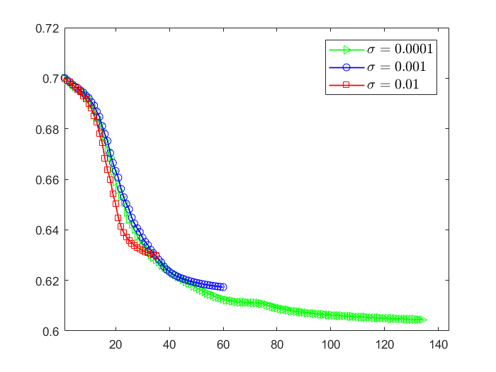
c

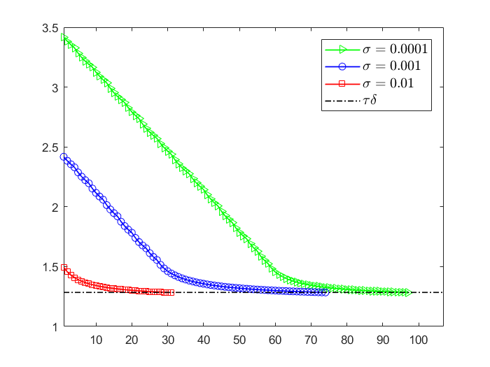
d

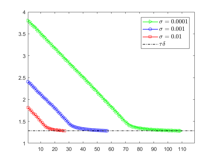
e

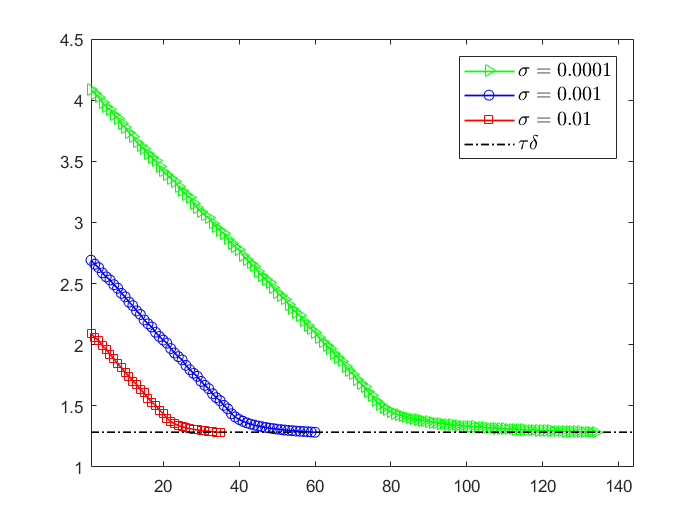
f

Figure 5: Logarithmic relative errors ($\displaystyle E_{n}$, top row) and logarithmic residuals ($\displaystyle R_{n}$, bottom row) for different noise levels: $\displaystyle\sigma=0.0001$, $\displaystyle\sigma=0.001$, and $\displaystyle\sigma=0.01$. From left to right: results for Example 1, Example 2 and Example 3.

Figure 5 illustrates the stability and convergence properties of the Iterative Regularizing Ensemble Kalman Method (IREKM) when applied to the inverse problem. As noise decreases, the approximation errors progressively diminish, demonstrating the method’s robustness. The stopping criterion, based on the residual $\displaystyle R_{n}$, ensures proper algorithm termination by enforcing the condition $\displaystyle R_{n}\leq\tau\delta$, where $\displaystyle\delta$ quantifies the noise level. This avoids overfitting and ensures convergence. The plotted residuals confirm the correct implementation of the stopping criterion, as the errors consistently decrease throughout the iterations. Additionally, the figures demonstrate that both the error and residual stabilize after a few iterations, indicating rapid convergence to an acceptable solution. Notably, when noise levels are lower, the algorithm requires more iterations to meet the stopping criterion. This is because achieving higher precision in low-noise scenarios demands further refinement of the solution, requiring additional computational steps to reduce the residual to the desired threshold.

In conclusion, the Iterative Regularizing Ensemble Kalman Method (IREKM) proves to be a robust and efficient approach for solving the inverse problem of identifying diffusion terms in the HIV infection model. The method exhibits strong stability and convergence properties, as approximation errors decrease with lower noise levels. Furthermore, IREKM shows notable sensitivity to noise, yielding precise reconstructions, particularly in low-noise scenarios.

5 Concluding Remarks

In this study, we investigated an inverse problem associated with a time-fractional HIV infection model incorporating nonlinear diffusion. Our primary objective was to recover unknown diffusion functions using final time measurement data. Given the ill-posedness of the inverse problem and the presence of measurement noise, we employed a Bayesian inference framework combined with the Iterative Regularizing Ensemble Kalman Method (IREKM) to achieve stable and reliable reconstructions. The numerical experiments demonstrated the effectiveness of the proposed methodology in reconstructing the unknown diffusion terms under various noise levels. The results indicated that the IREKM method successfully captured the complex diffusion dynamics of the HIV infection model while maintaining robustness against observational noise. Furthermore, the Bayesian approach allowed for uncertainty quantification, providing a comprehensive assessment of the estimated parameters.

Key findings from this research include:

1. The proposed framework is capable of accurately recovering nonlinear diffusion terms in the HIV infection model, even under moderate noise conditions.

2. The stability and convergence of the method were validated through multiple test cases, showing improved performance as noise levels decreased.

3. The sensitivity analysis confirmed that IREKM is effective in handling inverse problems for nonlocal and nonlinear models, making it a promising tool for studying complex biological systems.

While the proposed approach demonstrates strong performance, several directions for future research remain. Extending the method to higher-dimensional problems and incorporating real experimental data could offer additional insights into HIV infection dynamics. Furthermore, improving computational efficiency, particularly for large-scale simulations, remains an important area for development. Lastly, exploring alternative regularization techniques may further enhance the robustness of the inverse problem formulation. Overall, this study contributes to the growing field of inverse problems in fractional differential models and provides a computational framework to advance the understanding of HIV infection mechanisms.

References

- [1] X. Ren, Y. Tian, L. Liu, X. Liu. A reaction-diffusion within-host HIV model with cell - cell transmission. J. Math. Biology, 76, 1831-1872, 2018.
- [2] A. Babaei, H. Jafari , A. Liya. Mathematical models of HIV/AIDS and drug addiction in prisons. Eur. Phys. J. Plus, 135, 395, 2020.
- [3] K.O. Okosun, O.D. Makinde , I. Takaidza. Impact of optimal control on the treatment of HIV/AIDS and screening of unaware infectives. App. Math. Model., 37, 3802-3820, 2013.
- [4] R.M. Anderson, G.F. Medley , R.M. May, A.M. Johnson. A Preliminary Study of the Transmission Dynamics of the Human Immunodeficiency Virus (HIV), the Causative Agent of AIDS. IMA Journal of Mathematics Applied in Medicine Biology, 3, 229-263, 1986.
- [5] M.H. Ostadzad, G.H. Erjaee. Dynamical analysis of public health education on HIV/AIDS transmission. Math. Methods in the App. Sci., 38, 3601-3614, 2014.
- [6] C. Connell McCluskey. A model of HIV/AIDS with staged progression and amelioration. Mathematical Biosciences, 181, 1-16, 2003.
- [7] ARM. Carvalho, CMA. Pinto. Emergence of drug-resistance in HIV dynamics under distinct HAART regimes. Commun. Nonlinear. Sci. Numer. Simulat., 30, 207-226, 2016.
- [8] V.D. Djordjevic , J. Jaric, B. Fabry, JJ. Fredberg, D. Stamenovic. Fractional derivatives embody essential features of cell rheological behavior. Ann. Biomed. Eng., 31, 692-699, 2003.
- [9] T. J. Anastasio. The fractional-order dynamics of brainstem vestibulo-oculomotor neurons. Biol. Cybern., 72, 69-79, 1994
- [10] I. Petras, IR. Magin. Simulation of drug uptake in a two compartmental fractional model for a biological system. Commun. Nonlinear. Sci. Numer. Simulat., 16, 4588-4595, 2011
- [11] Y. Ding, H. Ye. A fractional-order differential equation model of hiv infection of -cells. Math. Comput. Model., 50, 386-392, 2009.
- [12] Y. Ding, Z. Wang, H. Ye. Optimal control of a fractional-order HIV-immune system with memory. IEEE Trans. Control Syst. Technol., 20, 763-769, 2012.
- [13] CMA. Pinto, ARM. Carvalho. New findings on the dynamics of HIV and TB coinfection models. Appl. Math. Comput., 242, 36-46, 2014.
- [14] CMA. Pinto, ARM. Carvalho. A latency fractional order model for HIV dynamics. J. Comput. Appl. Math. , 312, 240-256, 2017.
- [15] A. Jajarmi, D. Baleanu. A new fractional analysis on the interaction of HIV with T-cells. Chaos Soliton Frac., 113, 221-229, 2018.
- [16] A. Babaei, H. Jafari, M. Ahmadi. A fractional order HIV/AIDS model based on the effect of screening of unaware infectives. Math. Meth. Appl. Sci. , 1-10, 2019, https://doi.org/10.1002/mma.5511.
- [17] F. Mainardi. Fractional relaxation-oscillation and fractional diffusion-wave phenomena. Chaos Soliton Frac., 7, 1461-1477, 1996.
- [18] J. Manimaran, L. Shangerganesh, A. Debbouche, J.-C. Cortés. A time-fractional HIV infection model with nonlinear diffusion. Results in Physics, 25, 104293, 2021.
- [19] J. Cheng, J. Nakagawa, M. Yamamoto, T. Yamazaki. Uniqueness in an inverse problem for a one-dimensional fractional diffusion equation. Inverse Problems, 25, 115-131, 2009.
- [20] B. Jin, W. Rundell. An inverse problem for a one-dimensional time-fractional diffusion problem. Inverse Problems, 28, 075010, 2012.
- [21] J.J. Liu, M. Yamamoto. A backward problem for the time-fractional diffusion equation. Applicable Analysis, 89, 1769-1788, 2010.
- [22] K. Sakamoto, M. Yamamoto. Inverse source problem with a final overdetermination for a fractional diffusion equation. Mathematical Controls and Related Fields, 4, 509–518, 2011.
- [23] K. Sakamoto, M. Yamamoto. Initial value/boundary value problems for fractional diffusion-wave equations and applications to some inverse problems. Journal of Mathematical Analysis and Applications, 382, 426-447, 2011.
- [24] X. Xu, J. Cheng, M. Yamamoto. Carleman esimate for a fractional diffusion equation with half order and application. Applicable Analysis, 90, 1355-1371, 2011.
- [25] Y. Zhang, X. Xu. Inverse source problem for a fractional diffusion equation. Inverse Problems, 27, 035010, 2011.
- [26] S. Tatar, S. Ulusoy. A uniqueness result in an inverse problem for a space-time fractional diffusion equation. Electron. J. Differ. Equ, 258, 1-9, 2013.
- [27] S. Tatar, R. Tinaztepe, S. Ulusoy. Simultaneous inversion for the exponents of the fractional time and space derivatives in the space-time fractional diffusion equation. Applicable Analys., 95, 1-23, 2016.
- [28] N.H. Tuan, T.B. Ngoc, S. Tatar, L.D. Long. Recovery of the solute concentration and dispersion flux in an inhomogeneous time fractional diffusion equation. Journal of Comp. and Appl. Math., 342, 96-118, 2018.
- [29] N.H. Tuan, L.D. Long, S. Tatar. Tikhonov regularization method for a backward problem for the inhomogeneous time-fractional diffusion equation. Applicable Analysis, 97, 842-863, 2018.
- [30] G. Li, D. Zhang, X. Jia, M. Yamamoto Simultaneous inversion for the space-dependent diffusion coefficient and the fractional order in the time fractional diffusion equation. Inverse Problems, 29, 065014, 2013.
- [31] S. Tatar, R. Tinaztepe, S. Ulusoy. Determination of an unknown source term in a space-time fractional diffusion equation. Journal of Fractional Calculus Applications, 6, 83-90, 2015.
- [32] S. Tatar, S. Ulusoy. Analysis of Direct and Inverse Problems for a Fractional Elastoplasticity Model. Filomat, 31, 699-708, 2017.
- [33] S. Tatar, S. Ulusoy. An inverse problem for a nonlinear diffusion equation with time-fractional derivative. Journal of Inverse and Ill-posed Prob., 25, 185-193, 2017.
- [34] S. Tatar, R. Tinaztepe, M. Zeki. Numerical Solutions of Direct and Inverse Problems for a Time Fractional Viscoelastoplastic Equation. Journal of Engineering Mechanics, 143, 2017, DOI: 10.1061/(ASCE)EM.1943-7889.0001239.
- [35] M. Zeki, R. Tinaztepe, S. Tatar, S. Ulusoy, R. Al-Hajj. Determination of a Nonlinear Coefficient in a Time-Fractional Diffusion Equation. fractal and fractional, 7, 2023, https://doi.org/ 10.3390/fractalfract7050371.
- [36] M. Zeki, S. Tatar. An iterative approach for numerical solution to the time-fractional Richards equation with implicit Neumann boundary conditions. Europ. J. of. Pure and Appl. Mathematics, 16, 491-502, 2023.
- [37] N.H. Tuan, L.V.C. Hoan, S. Tatar. An inverse problem for an inhomogeneous time-fractional diffusion equation: a regularization method and error estimate. Applicable Analysis, 38, 2019, https://doi.org/10.1007/s40314-019-0776-x.
- [38] A. A. Kilbas, H. M. Srivastava and J. J. Trujillo. Theory and Applications of Fractional Differential Equations. Elsevier, Amsterdam, 2006.
- [39] I. Podlubny. Fractional Differential Equations. Academic Press, San Diego, 1999.
- [40] L. Boccardo, A. Dall’Aglio, T. Gallouët, L. Orsina Nonlinear Parabolic Equations with Measure Data. Journal of Func. Analysis, 147 237-258, 1997.
- [41] J. Manimaran, L. Shangerganesh, A. Debbouche,V. Antonov Numerical Solutions for Time-Fractional Cancer Invasion System With Nonlocal Diffusion Front. Phys., 7:93, 2019.
- [42] N. G. Trillos, D. Sanz-Alonso. The Bayesian formulation and well-posedness of elliptic inverse problems. Inverse Problems 33 065006, 2017.
- [43] N. K. Chada, M. A. Iglesias, L. Roininen, A. M. Stuart. Parameterizations for ensemble Kalman inversion. Inverse Problems, 34(5):055009, 2018.
- [44] S. L. Cotter, M. Dashti, A. M. Stuart. Approximation of Bayesian inverse problems for PDEs. SIAM Journal on Numerical Analysis, 48(1):322–345, 2010.
- [45] M. Dashti, A. M. Stuart. Uncertainty quantification and weak approximation of an elliptic inverse problem. SIAM Journal on Numerical Analysis, 49(6):2524–2542, 2011.
- [46] M. A. Iglesias. A regularizing iterative ensemble Kalman method for PDE-constrained inverse problems. Inverse Problems, 32(2):025002, 2016.
- [47] M. A. Iglesias, K. Lin, S. Lu, A. M. Stuart. Filter based methods for statistical linear inverse problems. Communications in Mathematical Sciences, 15(7), 1867-1896, 2017.
- [48] J. Kaipio, E. Somersalo. Statistical and computational inverse problems. Springer Science & Business Media, volume 160, 2006.
- [49] A. M. Stuart. Inverse problems: a Bayesian perspective. Acta Numerica, 19:451–559, 2010.
- [50] L. Yan, Y.-X. Zhang. Convergence analysis of surrogate-based methods for Bayesian inverse problems. Inverse Problems, 33(12):125001, 2017.
- [51] L. Yan, T. Zhou. An adaptive multifidelity PC-based ensemble Kalman inversion for inverse problems. International Journal for Uncertainty Quantification, 9(3), 2019.
- [52] L. Yan, T. Zhou. Adaptive multi-fidelity polynomial chaos approach to Bayesian inference in inverse problems. Journal of Computational Physics, 381:110–128, 2019.
- [53] M. A. Iglesias. Iterative regularization for ensemble data assimilation in reservoir models. Computational Geosciences, 19:177–212, 2015.
- [54] Y.-X. Zhang, J. Jia, L. Yan. Bayesian approach to a nonlinear inverse problem for a time-space fractional diffusion equation. Inverse Problems, 34(12):125002, 2018.
- [55] G. Evensen. Analysis of iterative ensemble smoothers for solving inverse problems. Computational Geosciences, 22(3):885–908, 2018.
- [56] M. A. Iglesias, K. J. H. Law, A. M. Stuart. Ensemble Kalman methods for inverse problems. Inverse Problems, 29(4):045001, 2013.
- [57] C. Schillings, A. M. Stuart. Convergence analysis of ensemble Kalman inversion: the linear, noisy case. Applicable Analysis, 97(1):107-123, 2018.
- [58] Y. Lin, C. Xu. Finite difference/spectral approximations for the time-fractional diffusion equation. J. Comput. Phys., 225(2), 1533-1552, 2007.
- [59] M. BenSalah, H. Maatoug. Inverse source problem for a space-time fractional diffusion equation. Ricerche di Mat., 73(4), 681-713, 2024.
- [60] M. BenSalah. Shape and location recovery of laser excitation sources in photoacoustic imaging using topological gradient optimization. J. Comput. Appl. Math., 451, 116047, 2024.