Predicting the von Neumann Entanglement Entropy Using a Graph Neural Network

Abstract

Calculating the von Neumann entanglement entropy from experimental data is challenging due to its dependence on the complete wavefunction, forcing reliance on approximations like classical mutual information (MI). We propose a machine learning approach using a graph neural network for predicting the von Neumann entropy from experimentally accessible bitstrings. We tested this approach on a Rydberg ladder system and achieved a mean absolute error of $3.7\times 10^{-3}$ when testing it inside of its training range on a dataset with entropy ranging from 0 to 1.9, we also evaluated the mean absolute percentage error on the data that have its entropy larger than 0.01 of the maximum entropy(so we can avoid the areas of our phase space with near zero entropy) and got a relative error of 1.72%, outperforming MI-based bounds. When tested beyond this range, the model still delivers reasonable results. Furthermore, we demonstrate that fine tuning the model with a small dataset significantly improves its performance on data outside its original training range.

I Introduction

Quantum entanglement is a cornerstone of quantum mechanics, and the von Neumann entanglement entropy serves as a key measure of entanglement with broad applications across physics. This entropy is defined as

$$S^{vN}_{A}=-Tr(\rho_{A}\ln(\rho_{A})),$$ (1)

where $\rho_{A}=Tr_{B}\rho_{AB}$ is the reduced density matrix of subsystem A. However, calculating $S^{vN}_{A}$ typically requires knowledge of the full quantum wavefunction, which is not directly accessible from experimental measurements alone.

A recent work has addressed this challenge for a Rydberg ladder system by demonstrating that a lower bound for $S^{vN}_{A}$ can be estimated experimentally using the classical mutual information (MI) derived from easily available bitstrings [1]. In this study, we propose a graph neural network (GNN) model to estimate $S^{vN}_{A}$ directly from the same experimental data used for MI calculations. Our approach bypasses the need for full wavefunction reconstruction and leverages correlations in the bitstrings to infer entanglement properties.

GNNs provide a natural framework for modeling quantum systems: nodes represent individual particles, while edges encode correlations and interactions. This graph structure mirrors the physical interactions governing entanglement, enabling the network to infer $S^{vN}_{A}$ without wavefunction reconstruction.

The paper is structured as follows: Section 2 reviews machine learning in quantum physics and GNNs, section 3 details our methodology (including data generation and model architecture), In section 4 we go over our results and show how fine tuning the model could work after the initial training is done.

II Background

II.1 Machine Learning for Quantum Systems

The intersection of machine learning (ML) and quantum physics has emerged as a groundbreaking frontier, offering novel solutions to problems once deemed intractable due to the inherent complexity of quantum systems. Quantum mechanics, governed by principles such as superposition, entanglement, and exponential state-space scaling, poses unique challenges for both theoretical modeling and experimental data analysis. Traditional computational methods, such as exact diagonalization or quantum Monte Carlo, often struggle with the ”curse of dimensionality” in many-body systems or the noise susceptibility of quantum hardware. Machine learning, with its capacity to approximate high-dimensional functions, extract patterns from sparse data, and optimize complex systems, has become an indispensable tool in advancing quantum research[2].

In quantum many-body physics, neural networks have revolutionized the representation of wavefunctions. For instance, neural quantum states (NQS) leverage deep learning architectures to approximate ground and excited states of correlated quantum systems, bypassing the limitations of conventional variational methods. These approaches have enabled precise simulations of spin lattices, fermionic systems, and quantum phase transitions[3], [4].

Quantum computing has also benefited from ML, in [5] it was shown that a neural-network-based reinforcement learning (RL) can discover quantum error correction (QEC) strategies for protecting logical qubits against noise in few-qubit systems.

Meanwhile, generative models like quantum autoencoders assist in quantum error correction which leads to extending the lifetime of logical qubits[6]. These advances are critical for bridging the gap between theoretical quantum advantage and practical implementation.

II.2 Graph Neural Networks in Physics

Graph Neural Networks have emerged as a powerful framework for modeling systems with inherent relational or topological structure, such as atomic lattices, particle interaction networks, and much more. Unlike traditional neural architectures, GNNs operate directly on graph-structured data, leveraging message-passing mechanisms to propagate and aggregate information between nodes and edges. This capability aligns naturally with physics problems where locality, symmetry, and connectivity play defining roles, such as in material science, quantum chemistry, and particle physics [7].

Some examples of GNNs use in physics include predicting material properties in condensed matter physics, as it’s especially suited for such tasks[8], and top tagging as discussed in[9]

III Methodology

III.1 Dataset

In this work, we study a Rydberg system described by the following Hamiltonian:

$$\begin{split}H\;=\;\frac{\Omega}{2}\sum_{i}\biggl{(}e^{i\phi}\,\lvert g\rangle_{i}\langle e\rvert_{i}\;+\;e^{-i\phi}\,\lvert e\rangle_{i}\langle g\rvert_{i}\biggr{)}\\ \;-\;\Delta(t)\sum_{i}\hat{n}_{i}\;+\;\sum_{i<j}\frac{C_{6}}{\lvert\vec{r}_{i}-\vec{r}_{j}\rvert^{6}}\,\hat{n}_{i}\hat{n}_{j}\,.\end{split}$$ (2)

Where $C_{6}=5.42\times 10^{-24}\frac{m^{6}}{s}rad$, $\Omega$ is the Rabi drive amplitude, and $\Delta$ is the detuning.

The atoms are arranged in a two-leg ladder configuration, with the y-separation being twice the x-separation. This system is based on the Aquila quantum computer developed by QuEra.

To generate our dataset, we randomly sampled specific ranges of the Hamiltonian parameters. Instead of sampling over $\Delta$, $\Omega$ , and $a$(where $a$ is the lattice x-spacing). We normalized our Hamiltonian by dividing by $\Omega$. We then sampled the dimensionless ratios $\frac{\Delta}{\Omega}$ and $\frac{R_{b}}{a}$, where $Rb$ is defined as $R_{b}=(\frac{C_{6}}{\Omega})^{\frac{1}{6}}$. Additionally, we sampled the number of rungs(ladder legs) in the system. The sampling ranges were as follows:

$$\begin{split}\frac{\Delta}{\Omega}\in[0,6],\\ \frac{R_{b}}{a}\in[0.1,5],\\ N_{rungs}\in[1,6].\end{split}$$ (3)

The number of samples taken for $\frac{\Delta}{\Omega}$ and $\frac{R_{b}}{a}$ were evenly distributed. However, for the number of rungs, we increased the number of samples for larger systems to account for the growing complexity with system size. Specifically, the number of samples for rungs 1 through 6 was $30000,60000,100000,200000,350000,500000$ respectively..
For each sample, we diagonalized the Hamiltonian, computed the ground state, randomly selected a subsystem, and calculated the von Neumann entanglement entropy.

III.2 Preprocessing

Each data point was transformed into a graph, where nodes represent the Rydberg atoms, and edges represent the interactions between these atoms. We then defined a set of experimentally accessible features for the nodes, edges, and the graph as a whole.

III.2.1 Node Features

For each node, we assigned the following features:

• Coordinates: The atoms were placed on a grid with $x$-spacing = 1 and $y$-spacing = 2.

• Rydberg State Probability: The probability of the atom being in the Rydberg state, calculated using the ground state probabilities.

• Subsystem Mask: A binary value indicating whether the node belongs to subsystem ’A’ or ’B’.

III.2.2 Edge Features

We created edges between any two nodes within a distance of 6 units to capture short- and medium-range interactions, while ignoring long-range interactions that contribute negligibly to the quantum state. For each edge, we defined the following features:

• Normalized Distance: The distance between the connected nodes divided by the square root of the total number of atoms.

• Angle with Horizontal Axis: The angle that the edge makes with the horizontal axis.

• Two-Point Correlation: Defined as $C_{ij}=\langle r_{i}r_{j}\rangle-\langle r_{i}\rangle\langle r_{j}\rangle$.

The first two features were chosen to encode the geometric structure of the system, while the third feature captures the correlations between Rydberg atoms.

III.2.3 Global Features

Finally, we defined two global features for the graph:

• $n_{A}$: The fraction of the system in subsystem ’A’.

• $n_{B}$: The fraction of the system in subsystem ’B’.

We can see in Fig. 1 the graph representation of a point with 2 rungs.
We found that this set of features effectively captures the relationships between the atoms and the entanglement entropy, while avoiding unnecessary complexity that could overwhelm the model.

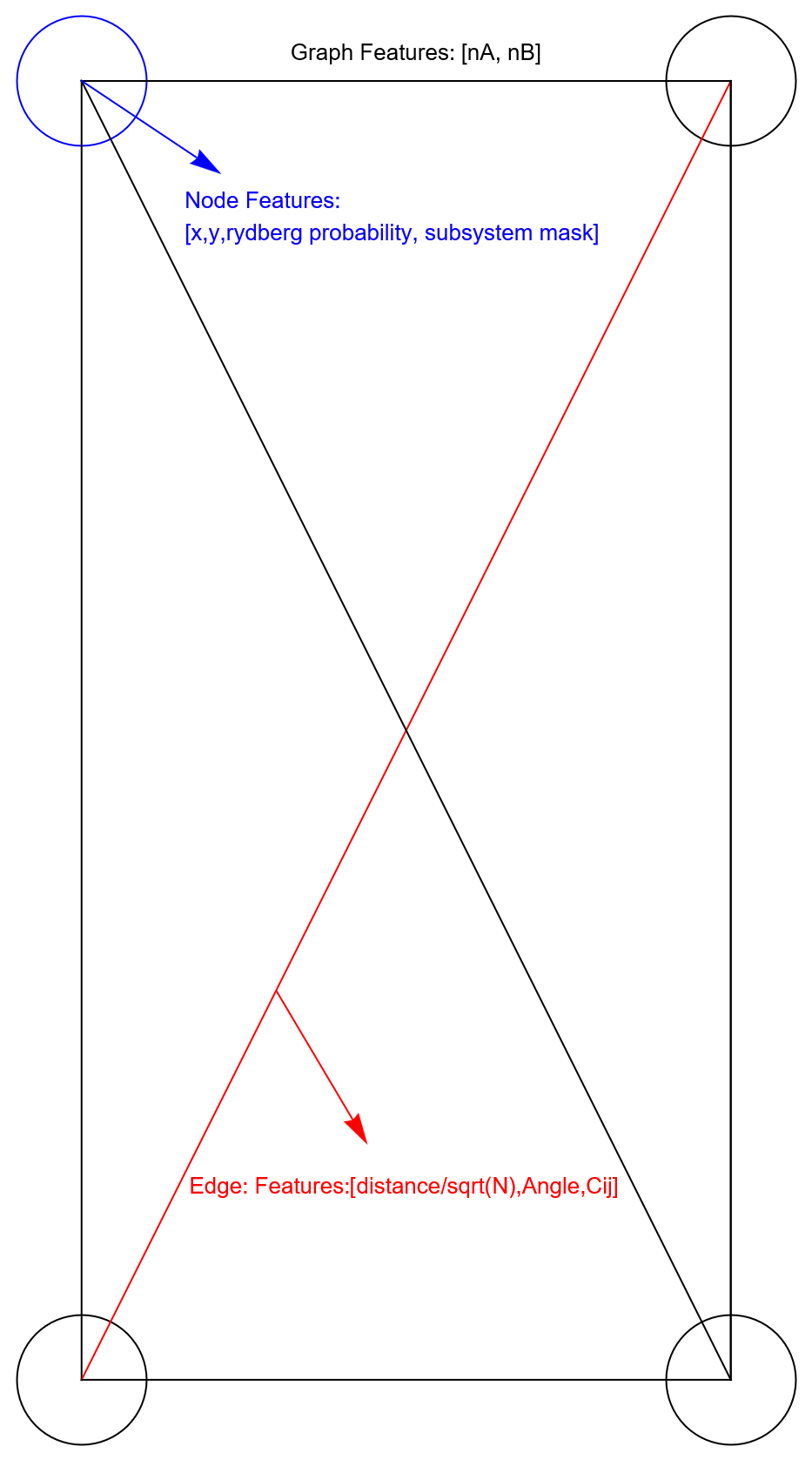
Figure 1: An example of how a 2-rung data point is represented after preprocessing.

III.3 Model Architecture

Our model is constructed using PyTorch geometric library, it consist of

III.3.1 Node & Edge Encoding

We implement node and edge encoders as 2-layer multilayer perceptrons (MLPs) with BatchNorm and SiLU (Sigmoid Linear Unit) activation. Each MLP transforms the input features (4-dimensional for nodes, 3-dimensional for edges) to a hidden representation of dimension 512

III.3.2 Edge Attention Layers

Here We introduce a MLP designed to give the model learnable weights for the importance of separate edges. The edge attention mechanism consists of a 3-layer MLP applied at each message passing layer, producing attention weights in the range [0, 1] through a sigmoid activation.

III.3.3 Edge Representation MLP

Here We take the output of the edge encoding MLP as an input and output another edge representation consisting of 2 layers, BatchNorm, SiLU activation and dropout.

III.3.4 Message Passing Layers

We implement a multi-layer architecture for edge-node co-processing, alternating between two distinct message passing mechanisms across 6 layers. For even-indexed layers, we employ GINEConv[10] operations with enhanced edge features. Each GINEConv utilizes a 3-layer MLP that processes node representations, consisting of two linear transformations with BatchNorm, SiLU activation, and dropout (p=0.4) in between. For odd-indexed layers, we leverage TransformerConv[11] operations with edge-aware attention mechanisms. Each TransformerConv implements multi-head attention with 8 attention heads, where each head processes features of dimension 64. The TransformerConv incorporates beta-transformations and concatenates the outputs from different attention heads. Both convolution types incorporate edge features multiplied by thier weights of dimension 512 to guide the message passing process, enabling rich interactions between node and edge representations throughout the network.
Residual connections are added after each message passing layer to stabilize training and improve gradient flow. Specifically, the output of each convolution operation $h_{new}$ is added to the previous node features $h$.
After every even-indexed message passing layer, we apply an intermediate processing step to further refine the node features. This step consists of a 2-layer MLP with BatchNorm, SiLU activation, and dropout. The MLP transforms the node features while preserving their dimensionality, allowing for additional feature extraction and regularization.
And at the end of each message passing layer we update the edge representation and weights using separate MLP’s and take the updated representations as an input for the next message passing layer.

III.3.5 Graph-Level Readout

For getting a graph-level readout, we implement a multi-head readout mechanism using two Set2Set modules with 4 processing steps each.
To manage the increased dimensionality from the multi-head readout (2048), we employ a dimension reduction projection. This projection consists of a linear transformation followed by BatchNorm, SiLU activation, and dropout regularization, reducing the representation to 1024.

III.3.6 Global Features MLP

We add an MLP consisting of three layers, BatchNorm, SiLU activation, and dropout to process the global features.

III.3.7 Final MLP

The final MLP combines the graph-level readout and the global features MLP output, producing a single scalar value representing the von Neumann entropy. The final MLP consists of four layers with BatchNorm, SiLU activation, and dropout, followed by a Softplus activation to ensure non-negative output.

A flow chart of the model is shown in Fig. 2.

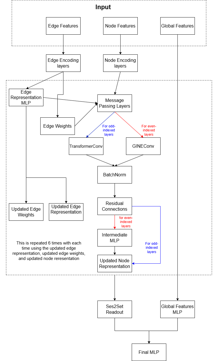
Figure 2: A flow chart of the GNN model.

III.4 Training

We trained the model over 500 epochs using the Kaiming initialization[12], we used the AdamW optimaizer[13] with learning rate equal to $1.5\times 10^{-4}$ and a weight decay of $10^{-4}$. To stabilize training, we applied gradient clipping with a maximum gradient norm of 1.0. We also used the CosineAnnealingWarmRestarts scheduler[14] with the following parameters, $T_{0}=50$, $T_{mult}=2$, and $\eta_{min}=10^{-6}$. The exact values for the optimizer parameters, scheduler parameters, dropout rate, the dimensionality of the inner layer of the model, and the number of message passing layers were determined using an optimizing code that minimized our validation loss over a 100 epoch, we specifically used a Tree-structured Parzen Estimator[15] over those parameters and got the ones we used in the final training code.
As for the loss we defined a physics-based loss function that has 2 parts to it, the first is a Log-Cosh loss and the second part is a function that peanlized the model for predicting entropy outside the physically allowed values, $0\leq S_{v}\leq Min(N_{A},N_{B})\ln(2)$, the way we did this was

$$\begin{split}loss_{bounds}=\sum\frac{1}{4N}(ReLU(-S_{pred})\\ +ReLU(S_{pred}-Min(N_{A},N_{B})\ln(2))).\end{split}$$ (4)

Where $N_{A}$ and $N_{B}$ are the number of atoms in subsystem A and B respectively

IV Results

We used 3 metrics to evaluate our model, the first one is our loss defined as

$$loss=loss_{bounds}+\frac{1}{N}\sum\log(\cosh(S_{pred}-S)),$$ (5)

the second is the mean average error defined as

$$MAE=\frac{1}{N}\sum\left|S_{pred}-S\right|,$$ (6)

and the third is the mean absolute percentage error defined as

$$MAPE=\frac{100}{N}\sum\left|\frac{S_{pred}-S}{S}\right|.$$ (7)

But we only evaluated the MAPE of the points that had an actual entropy value higher than 0.01 of the maximum value in the dataset. This threshold approach prevents artificially inflated error metrics in regions of near-zero entropy, where even small absolute errors can result in disproportionately large percentage errors.

After training the model for 500 epochs, the model achieved a validation loss of $1.6\times 10^{-5}$ and a validation MAE of $3.7\times 10^{-3}$. We ran an evaluation of the entire dataset after training and recorded the results in table 1 and 2, and plotted it in Fig. 3.

Table 1: List of the mean average error for each system size

System Size	MAE$\times 10^{-3}$	System Size	MAE$\times 10^{-3}$
2	8.783	8	3.088
4	4.346	10	3.259
6	2.957	12	4.017

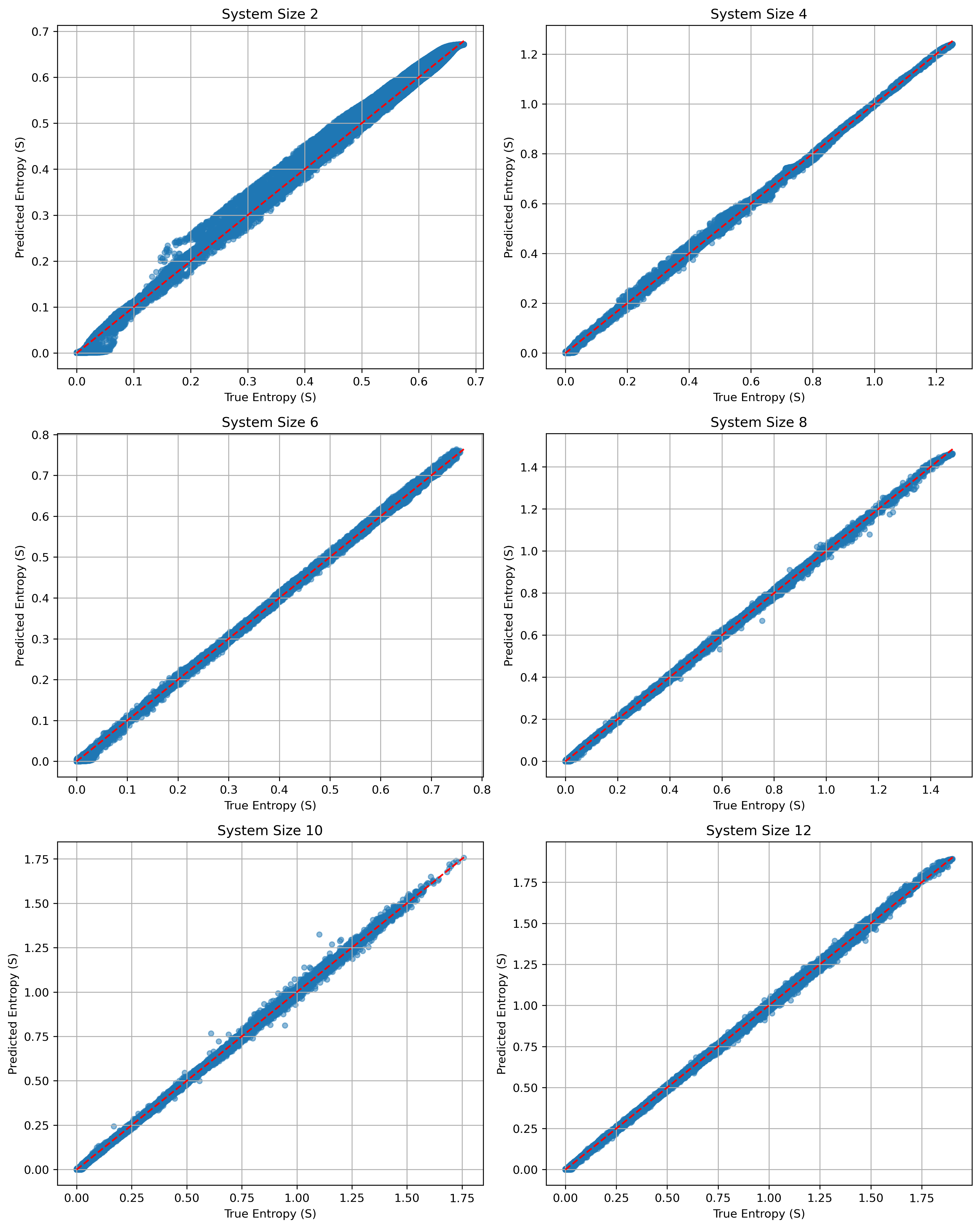
Figure 3: Predicted vs. actual von Neumann entanglement entropy.

Table 2: List of the mean absolute percentage error for each system size

System Size	MAPE	System Size	MAPE
2	3.22%	8	0.95%
4	1.31%	10	0.94%
6	1.26%	12	0.93%

We also wanted to see how well does the model works compared to the classical mutual information(MI) so we plotted in Fig. 4 the von Neumann entropy, MI and our model predictions in the phase space of $\frac{R_{b}}{a}$ and $\frac{\Delta}{\Omega}$ of a symmetrical partition of a 6-rung system.

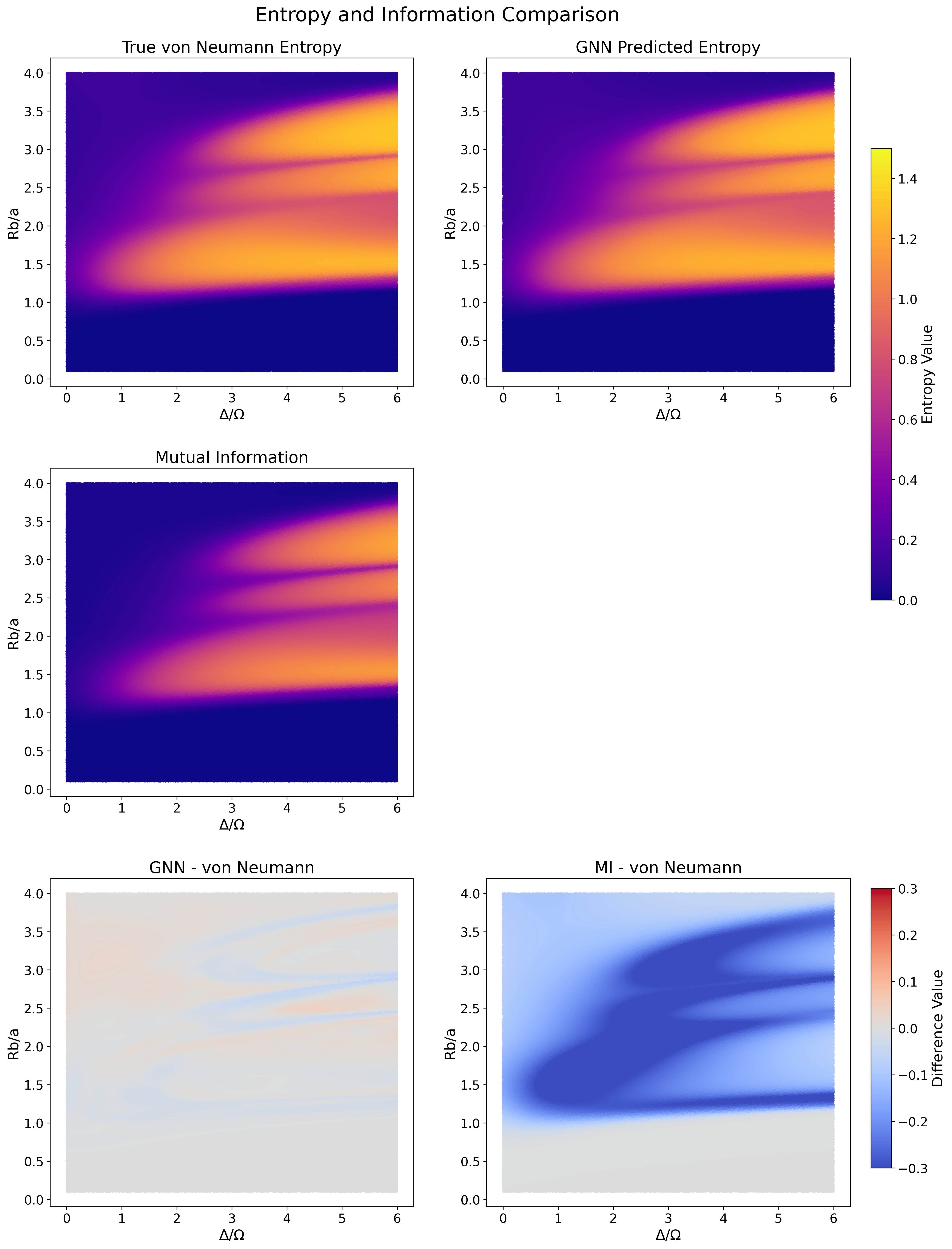
Figure 4: Heat maps of the von Neumann entropy, the GNN prediction, the MI, and the difference between them.

We also tested the model for robustness against small fluctuations in the input which is very important in any model that depend on experimental data, we did this by dropping any state with probability less than $10^{-4}$ and re-normalizing the wavefunction. We got a MAE of 0.010955 and a MAPE of 5.31% on the symmetric partition dataset, compared to the MAE and MAPE we got before truncating our wavefunction which are equal to 0.008766 and 3.64% respectively, our results can be seen in Fig. 5.

Figure 5: Heat maps of the GNN - von Neumann entropy, and the MI - von Neumann entropy after truncation.

Another important feature the model should have is it’s generalization, as generating data for more than 6 rungs in the same volumes we did to train the model gets computationally expensive fast, so we tested our model on datasets of 7-10 rungs at specific value for $\frac{\Delta}{\Omega}$, the results are shown in table 3 and 4.

IV.1 Fine Tuning the Model

While our model outperformed the MI for sizes larger than what it was trained on, the MAE is not as low as we would like. This issue can be solved by fine-tuning the model to the specific size we are interested in. We performed fine-tuning of the model weights for 7 and 8 rungs using a much smaller dataset of 10,000 samples compared to the original training dataset. We trained the model for 200 epochs using a $5\times 10^{-5}$ learning rate and $1.5\times 10^{-4}$ weight decay. We achieved a validation loss of $2.66\times 10^{-4}$ and MAE of $1.2183\times 10^{-2}$, which is a significant improvement over the original model. We plotted our results for a symmetrical partitions in Fig. 6 and the MAE and MAPE are listed in tables 3 and 4. We can clearly say that the model even improves its prediction for 9 and 10 rungs when it’s fine tuned for 7 and 8 rungs.

Table 3: Comparing the MAE for the original and fine tuned model

number of	$\frac{\Delta}{\Omega}$	MAE$\times 10^{-2}$	MAE$\times 10^{-2}$
rungs		(Original Model)	(Fine Tuned Model)
7	2.5	3.431	2.070
7	3.5	4.563	1.738
8	2.5	7.741	2.642
8	3.5	9.396	3.157
9	2.5	10.329	2.542
9	3.5	7.260	3.776
10	2.5	16.522	5.401
10	3.5	20.330	6.472

Table 4: Comparing the MAPE for the original and fine tuned model

number of	$\frac{\Delta}{\Omega}$	MAPE	MAPE
rungs		(Original Model)	(Fine Tuned Model)
7	2.5	18.15%	13.86%
7	3.5	20.80%	8.98%
8	2.5	16.51%	9.04%
8	3.5	16.97%	6.32%
9	2.5	31.10%	9.37%
9	3.5	16.77%	8.03%
10	2.5	33.21%	11.59%
10	3.5	28.81%	9.56%

Figure 6: von Neumann entropy(blue), the original model(red), the fine tuned model(purple), and the MI(green) as a function of $\frac{R_{b}}{a}$.

V Discussion & Conclusion

In this paper we suggested an architecture for a graph neural network model that takes in experimentally accessible data and predicts the von Neumann entanglement entropy. We tested this model on a Rydberg system like the one used in the Aquila quantum computer developed by QuEra.
Our model showed great results within its training range, with a mean average error of $3.7\times 10^{-3}$ and mean absolute percentage error of 1.72%. Testing the model outside of its training range also showed that the model predict the entropy somewhat well outside of its region but showed noticeable decrease in accuracy. This can be fixed by fine tuning the model for the specific size we are interested in using a small dataset. We showed this by starting with our base model and fine tuning it on 7 and 8 rungs, we saw significant improvements for our predictions for 7-10 rungs, this can be extended to any number of rungs by generating a small dataset using any appropriate approximation methods.

Code Availability

The codes used to generate the dataset, pre process it, train the model, and fine tune it, along with the weights of the original and fine tuned model are available on the github repository https://github.com/AsalehPhys/Predicting-von-Neumann-Entropy

References

- [1] Yannick Meurice. Experimental lower bounds on entanglement entropy without twin copy. arXiv preprint arXiv:2404.09935, 2024.
- [2] Giuseppe Carleo and Matthias Troyer. Solving the quantum many-body problem with artificial neural networks. Science, 355(6325):602–606, 2017.
- [3] Giuseppe Carleo, Ignacio Cirac, Kyle Cranmer, Laurent Daudet, Maria Schuld, Naftali Tishby, Leslie Vogt-Maranto, and Lenka Zdeborová. Machine learning and the physical sciences. Reviews of Modern Physics, 91(4):045002, 2019.
- [4] David Pfau, James S Spencer, Alexander GDG Matthews, and W Matthew C Foulkes. Ab initio solution of the many-electron schrödinger equation with deep neural networks. Physical review research, 2(3):033429, 2020.
- [5] Thomas Fösel, Petru Tighineanu, Talitha Weiss, and Florian Marquardt. Reinforcement learning with neural networks for quantum feedback. Physical Review X, 8(3):031084, 2018.
- [6] David F Locher, Lorenzo Cardarelli, and Markus Müller. Quantum error correction with quantum autoencoders. Quantum, 7:942, 2023.
- [7] Peter W Battaglia, Jessica B Hamrick, Victor Bapst, Alvaro Sanchez-Gonzalez, Vinicius Zambaldi, Mateusz Malinowski, Andrea Tacchetti, David Raposo, Adam Santoro, Ryan Faulkner, et al. Relational inductive biases, deep learning, and graph networks. arXiv preprint arXiv:1806.01261, 2018.
- [8] Tian Xie and Jeffrey C Grossman. Crystal graph convolutional neural networks for an accurate and interpretable prediction of material properties. Physical review letters, 120(14):145301, 2018.
- [9] Huilin Qu and Loukas Gouskos. Jet tagging via particle clouds. Physical Review D, 101(5):056019, 2020.
- [10] Weihua Hu, Bowen Liu, Joseph Gomes, Marinka Zitnik, Percy Liang, Vijay Pande, and Jure Leskovec. Strategies for pre-training graph neural networks. arXiv preprint arXiv:1905.12265, 2019.
- [11] Yunsheng Shi, Zhengjie Huang, Shikun Feng, Hui Zhong, Wenjin Wang, and Yu Sun. Masked label prediction: Unified message passing model for semi-supervised classification. arXiv preprint arXiv:2009.03509, 2020.
- [12] Kaiming He, Xiangyu Zhang, Shaoqing Ren, and Jian Sun. Delving deep into rectifiers: Surpassing human-level performance on imagenet classification. In Proceedings of the IEEE international conference on computer vision, pages 1026–1034, 2015.
- [13] Ilya Loshchilov and Frank Hutter. Decoupled weight decay regularization. arXiv preprint arXiv:1711.05101, 2017.
- [14] Ilya Loshchilov and Frank Hutter. Sgdr: Stochastic gradient descent with warm restarts. arXiv preprint arXiv:1608.03983, 2016.
- [15] James Bergstra, Rémi Bardenet, Yoshua Bengio, and Balázs Kégl. Algorithms for hyper-parameter optimization. Advances in neural information processing systems, 24, 2011.