A Class of Optimal Directed Graphs for Network Synchronization

Abstract

In a paper by Nishikawa and Motter, a quantity called the normalized spread of the Laplacian eigenvalues is used to measure the synchronizability of certain network dynamics. Through simulations, and without theoretical validation, it is conjectured that among all simple directed graphs with a fixed number of vertices and arcs, the optimal value of this quantity is achieved if the Laplacian spectrum satisfies a specific pattern. This paper proves that the conjectured Laplacian spectrum is always achievable by a class of almost regular directed graphs. For a few special cases, it is also shown that the corresponding value of the quantity is indeed optimal.

I The Conjecture

Over the past two decades, synchronization in complex networks has attracted considerable attention for its crucial role in fields including biology, climatology, ecology, sociology, and technology [1]. A typical class of network synchronization dynamics can be described as

$$\textstyle\dot{x}_{i}=F(x_{i})+\frac{\varepsilon}{d}\sum_{j=1}^{n}a_{ij}\big{(}H(x_{j})-H(x_{i})\big{)},$$ (1)

where $x_{i}$ is the state vector of the $i$th dynamical agent in a network of $n$ agents, $F$ represents the dynamics of each agent when isolated, $H(x_{j})$ denotes the signal that the $j$th agent sends to its neighboring agents, $a_{ij}$ is $ij$th entry of the adjacency matrix of the underlying simple directed graph, and $\varepsilon/d$ represents the coupling strength $\varepsilon$ normalized by the average coupling strength per vertex $d=\frac{1}{n}\sum_{i=1}^{n}\sum_{j=1}^{n}a_{ij}$. The network synchronization problem is to derive conditions under which all $n$ agents’ states converge to the same stable state. More details on the above network synchronization dynamics can be found in [2].

In the case when the underlying graph is undirected, the synchronizability of the network dynamics is measured by the eigenratio, which is defined as the ratio of the largest eigenvalue to the smallest nonzero eigenvalue of the Laplacian matrix [1, Section 4.1.2]. For directed graphs, however, there is no standard index for measuring synchronizability [1, page 115]. It is worth emphasizing that the network synchronization dynamics described in [1, Equation (54)] is mathematically equivalent to (1), although they use slightly different notation.

A directed graph is called simple if it does not have any self-arcs and multiple directed edges with the same tail and head vertices. For any simple directed graph $\mathbb{G}$ with $n$ vertices, we use $D$ and $A$ to denote its in-degree matrix and adjacency matrix, respectively. Specifically, $D$ is an $n\times n$ diagonal matrix whose $i$th diagonal entry equals the in-degree of vertex $i$, and $A$ is an $n\times n$ matrix whose $ij$th entry equals $1$ if $(j,i)$ is an arc (or a directed edge) in $\mathbb{G}$ and otherwise equals $0$. The Laplacian matrix of $\mathbb{G}$ is defined as $L=D-A$. It is easy to see that a Laplacian matrix $L$ always has an eigenvalue at 0 since all its row sums equal 0. In the special case when $\mathbb{G}$ is a simple undirected graph, each undirected edge between two vertices $i$ and $j$ can be equivalently replaced by a pair of directed edges $(i,j)$ and $(j,i)$; then $L$ is a symmetric matrix and thus has a real spectrum. It is well known that in this case $L$ is positive-semidefinite, its smallest eigenvalue equals 0, and its second smallest eigenvalue is positive if and only if $\mathbb{G}$ is connected [3]. For directed graphs, $L$ may have complex eigenvalues. Let $\lambda_{1},\lambda_{2},\ldots,\lambda_{n}$ denote all $n$ eigenvalues of $L$, with $\lambda_{1}=0$ and $\lambda_{2},\ldots,\lambda_{n}$ possibly complex. Define

$$\textstyle\sigma^{2}\stackrel{{\scriptstyle\Delta}}{{=}}\frac{1}{n-1}\sum_{i=2}^{n}|\lambda_{i}-\bar{\lambda}|^{2},\;\;{\rm where}\;\;\bar{\lambda}=\frac{1}{n-1}\sum_{i=2}^{n}\lambda_{i},$$

which is a normalized deviation of possibly nonzero eigenvalues. This quantity is called the normalized spread of the eigenvalues in [2] to measure the synchronizability of (1). It is claimed and validated by simulations that the smaller the value of $\sigma^{2}n^{2}/m^{2}$, the more synchronizable the network will generally be, where $m$ denotes the number of directed edges in $\mathbb{G}$. Note that since the sum of all $n$ agents’ in-degrees equals $m$ and the sum of all eigenvalues of a matrix equals the trace of the matrix, it follows that $\bar{\lambda}=m/(n-1)$ which is always a real number. It is clear that, for fixed values of $n$ and $m$, the smallest possible $\sigma^{2}$ corresponds to the optimal graph(s) for network synchronization. The following conjecture was proposed by Nishikawa and Motter in [2, Page 10343].

Conjecture: Among all simple directed graphs with $n$ vertices and $m$ arcs, the minimum possible value of $\sigma^{2}$ is

$$\textstyle\sigma^{2}_{\min}=\frac{1}{(n-1)^{2}}\big{[}m-(n-1)\kappa\big{]}\big{[}(n-1)(\kappa+1)-m\big{]},$$ (2)

which is achieved if the Laplacian spectrum is

$$0,\underbrace{\kappa,\;\ldots,\;\kappa,}_{(n-1)(\kappa+1)-m}\;\underbrace{\kappa+1,\ldots,\kappa+1}_{m-(n-1)\kappa},$$ (3)

where $\kappa\stackrel{{\scriptstyle\Delta}}{{=}}\lfloor\frac{m}{n-1}\rfloor$. Here $\lfloor\cdot\rfloor$ denotes the floor function.

Note that $\kappa$ is the unique integer such that $(n-1)\kappa\leq m<(n-1)(\kappa+1)$. Defining $q_{\kappa}=(n-1)\kappa$ and $q_{\kappa+1}=(n-1)(\kappa+1)$, it follows that $q_{\kappa}\leq m<q_{\kappa+1}$ and $\sigma_{\min}=(m-q_{\kappa})(q_{\kappa+1}-m)/(n-1)^{2}$, which is consistent with the expressions in [2]. It was implicitly assumed in [2] that $m\geq n-1$ for the conjecture, as indicated by its Fig. 2A where $m$ ranges from $n-1$ to $n(n-1)$. This assumption is natural, as network synchronization requires connectivity, and $n-1$ is the minimal number of arcs needed to guarantee a connected network. We will show that the conjecture holds when $m<n-1$ (cf. Section III-A).

It is worth emphasizing that the conjecture itself is independent of network synchronization dynamics, even though it was proposed as an optimal synchronization condition.

There is another popular way to define a Laplacian matrix of a directed graph based on out-degree [4]. Specifically, letting $D_{{\rm out}}$ denote the out-degree matrix of $\mathbb{G}$, the corresponding Laplacian matrix is denoted and defined as $L_{{\rm out}}=D_{{\rm out}}-A^{\prime}$. It is straightforward to verify that the in-degree Laplacian matrix of a directed graph $\mathbb{G}$ equals the out-degree Laplacian matrix of its transpose graph $\mathbb{G}^{\prime}$, where the transpose of a directed graph is the directed graph with the same vertex set obtained by reversing all its directed edges. In other words, $L(\mathbb{G})=L_{{\rm out}}(\mathbb{G}^{\prime})$. Since the set of all possible simple directed graphs with $n$ vertices and $m$ arcs is invariant under the graph transpose operation, the conjecture remains unaffected regardless of whether the Laplacian matrix is defined based on in-degree or out-degree. The only resulting difference is that any optimal graph with $\sigma_{\min}$ needs to be transposed if the definition is changed from in-degree based to out-degree based.

The conjecture was validated in [2] only for small-sized graphs with $n\leq 6$ through simulations; no theoretical validation was provided therein. Indeed, to the best of our knowledge, the conjecture has never been studied from a theoretical perspective. It even remains unclear whether the conjectured Laplacian spectrum (3) exists for a given fixed number of vertices $n$ and arcs $m$.

This paper shows that, for any feasible pair of $n$ and $m$, the conjectured Laplacian spectrum can always be achieved by a class of “almost regular” directed graphs. Therefore, all these graphs are conjectured optimal graphs for network synchronization. Furthermore, for any fixed number of vertices $n$, these graphs can be generated through an inductive construction algorithm for each possible number of arcs $m$. The paper also shows that the conjectured minimal normalized Laplacian eigenvalue spread is indeed the minimum in several special cases.

II The Algorithm

In this section, we present an algorithm that, for any fixed number of vertices $n>1$, inductively constructs a class of simple directed graphs, each having the Laplacian spectrum specified in (3) for every possible number of arcs $m\geq n-1$. To this end, we need the following concepts.

A vertex $i$ in a directed graph $\mathbb{G}$ is called a root of $\mathbb{G}$ if for each other vertex $j$ of $\mathbb{G}$, there is a directed path from $i$ to $j$. We say that $\mathbb{G}$ is rooted at vertex $i$ if $i$ is in fact a root, and that $\mathbb{G}$ is rooted if it possesses at least one root. In other words, a directed graph is rooted if it contains a directed spanning tree. An $n$-vertex directed tree is a rooted graph with $n-1$ arcs. It is easy to see that a directed tree has a unique root with an in-degree of $0$, while all other vertices have an in-degree of exactly $1$. The smallest possible directed tree is a single isolated vertex.

We use $a\bmod b$ to denote the modulo operation of two integers $a$ and $b$, which returns the remainder after dividing $a$ by $b$.

Algorithm 1: Given $n>1$ vertices, label them, without loss of generality, from $1$ to $n$. Let $\mathbb{G}(n,m)$ denote the $n$-vertex simple directed graph to be constructed with $m$ arcs. Start with the $m=n-1$ case and set $\mathbb{G}(n,n-1)$ as any directed tree such that all its arcs $(i,j)$ satisfy $i<j$. For each integer $n\leq m\leq n(n-1)$, compute $v_{n,m}=n-((m-1)\bmod n)$, identify the smallest index $u_{n,m}\in\{1,\ldots,n\}$ such that $u_{n,m}\neq v_{n,m}$ and $(u_{n,m},v_{n,m})$ is not an arc in $\mathbb{G}(n,m-1)$, then construct $\mathbb{G}(n,m)$ by adding the arc $(u_{n,m},v_{n,m})$ to $\mathbb{G}(n,m-1)$. $\Box$

The requirement $i<j$ for all arcs $(i,j)$ immediately implies that each directed tree $\mathbb{G}(n,n-1)$ is rooted at vertex $1$ and has vertex $n$ as a leaf. Before proceeding, we first show that the above algorithm is well defined.

Lemma 1

For any fixed $n>1$ and $n\leq m\leq n(n-1)$, the index $u_{n,m}$ defined in Algorithm 1 always exists.

Proof of Lemma 1: From the algorithm description, $\mathbb{G}(n,m)$ is constructed from $\mathbb{G}(n,m-1)$ by adding an arc with head index $v_{n,m}=n-((m-1)\bmod n)$. This process proceeds inductively from $m=n$ to $m=n(n-1)$. Note that for $n\leq m\leq n(n-1)$, the vertex index $v_{n,m}=n-((m-1)\bmod n)$ can take any value in $\{1,2,\ldots,n\}$. Each vertex in a graph with $n$ vertices has an in-degree of at most $n-1$. The algorithm begins with a directed tree, $\mathbb{G}(n,n-1)$, in which vertex $1$ has in-degree $0$, while all other vertices have an in-degree of $1$. Hence, to prove the existence of the vertex index $u_{n,m}$ described in the algorithm, it is sufficient to show that vertex $1$ appears as the head of an added arc (i.e., $v_{n,m}=1$ occurs) at most $n-1$ times during the inductive construction process, while each vertex $i\in\{2,\ldots,n\}$ appears as the head of an added arc (i.e., $v_{n,m}=i$ occurs) at most $n-2$ times. We thus consider vertex $1$ and vertices in $\{2,\ldots,n\}$ separately.

First consider vertex 1. The condition $v_{n,m}=n-((m-1)\bmod n)=1$ holds if and only if $m=kn$ with $k$ being any integer. Since $n\leq m\leq n(n-1)$, the condition occurs exactly $n-1$ times with $k\in\{1,\ldots,n-1\}$. Next consider vertices other than vertex 1. For each $i\in\{2,\ldots,n\}$, the condition $v_{n,m}=n-((m-1)\bmod n)=i$ holds if and only if $m=kn+1-i$ with $k$ being any integer. Since $n\leq m\leq n(n-1)$, the condition occurs exactly $n-2$ times with $k\in\{2,\ldots,n-1\}$.  

It is easy to see that the index $v_{n,m}\in\{1,\ldots,n\}$. With this, Lemma 1 ensures that Algorithm 1 operates without ambiguity under the given conditions for $n$ and $m$. In Figure 1, we present an illustrative example of the algorithm that inductively constructs a sequence of graphs $\mathbb{G}(n,m)$, where $n=6$ and $m$ ranges from $5$ to $16$. The first graph is a directed tree, and in each subsequent graph, a new arc is added to the preceding graph, with the newly added arc highlighted in purple. We will consistently use purple to indicate newly added arcs when illustrating an inductive construction process for Algorithm 1. For simplicity in drawing, we use a bidirectional edge to represent two arcs in opposite directions throughout this paper; each bidirectional edge is therefore counted as two arcs.

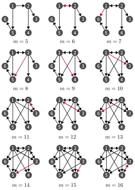
Figure 1: Inductive construction process of Algorithm 1 for $n=6$ and $5\leq m\leq 16$

From the algorithm description, the constructed graphs are all rooted simple directed graphs. Moreover, each constructed graph $\mathbb{G}(n,m)$, with $n\leq m\leq n(n-1)$, is dependent on the specific directed tree $\mathbb{G}(n,n-1)$. In other words, for any fixed $n$, each distinct directed tree $\mathbb{G}(n,n-1)$ uniquely determines a corresponding sequence of graphs $\mathbb{G}(n,m)$, $n\leq m\leq n(n-1)$.

We say that two directed graphs are identical if they have the same sets of vertices and arcs, with the same labels on both; this requirement is stronger than graph isomorphism. The classic Cayley’s formula [5] states that the number of distinct (undirected) trees on $n$ labeled vertices is $n^{n-2}$. Based on this, counting the number of distinct directed trees is easy. Any directed tree can be formed by orienting the edges of an undirected tree. Since each undirected tree allows any of its vertices to act as the root of a directed tree, each undirected tree can be oriented in $n$ different ways to form a directed tree. Therefore, the number of distinct directed trees on $n$ labeled vertices is $n\times n^{n-2}=n^{n-1}$. But this number cannot be used to count the total number of possible directed trees $\mathbb{G}(n,n-1)$, as the algorithm requires that all arcs $(i,j)$ in $\mathbb{G}(n,n-1)$ satisfy $i<j$.

Lemma 2

The number of distinct directed trees on $n$ labeled vertices, such that each arc $(i,j)$ satisfies $i<j$, is $(n-1)!$.

Proof of Lemma 2: We prove the lemma by induction on $n$. For the base case $n=1$, the lemma is clearly true. For the inductive step, suppose that the lemma holds for $n=k$, where $k$ is a positive integer. Let $n=k+1$. Since each arc $(i,j)$ is required to satisfy $i<j$, vertex $k+1$ must be a leaf vertex, and its parent vertex can be any vertex in $\{1,\ldots,k\}$. Thus, for each directed tree with $k$ vertices that satisfies the requirement, there are $k$ different ways to construct a directed tree with $k+1$ vertices that also satisfies the requirement by adding vertex $k+1$ as a child of any existing vertex. By the inductive hypothesis, the total number of desired directed trees with $k$ vertices is $(k-1)!$. Therefore, the total number of such directed trees with $k+1$ vertices equals $k\times(k-1)!=k!$, which proves the inductive step.  

The lemma states that there are $(n-1)!$ different possible $\mathbb{G}(n,n-1)$. That is to say, each $\mathbb{G}(n,m)$ may represent up to $(n-1)!$ different graphs. For simplicity, we use the notation as is and take this fact without further mention in the sequel. It is possible that, for certain values of $n$ and $m$, the graph $\mathbb{G}(n,m)$ constructed by the algorithm may be identical, even when the construction process begins with different directed trees. A trivial example is when $m=n(n-1)$ with which $\mathbb{G}(n,m)$ must be the complete graph regardless of $\mathbb{G}(n,n-1)$. Another illustrative $4$-vertex example is given in Figure 2. Moreover, a condition on the relationship between $n$ and $m$ is given in Lemma 7, which guarantees that $\mathbb{G}(n,m)$ is unique no matter what the initial tree is.

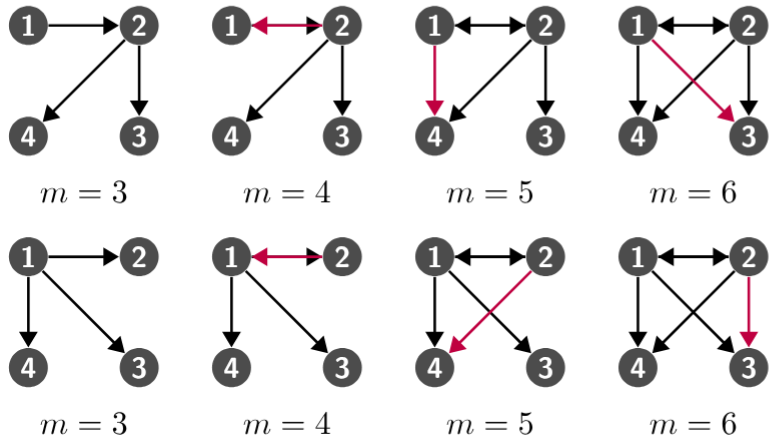
Figure 2: Two inductive construction processes (first row and second row), starting from different directed trees and leading to the identical $\mathbb{G}(4,6)$ graph

All constructed $\mathbb{G}(n,m)$ graphs have the following property. A directed graph is called almost regular if the difference between its largest and smallest in-degrees is at most $1$. In the special case when all in-degrees are equal, the graph is called regular. Let $\nu\stackrel{{\scriptstyle\Delta}}{{=}}\lfloor\frac{m}{n}\rfloor$.

Proposition 1

For any integers $n\geq 2$ and $m\geq n-1$, any $\mathbb{G}(n,m)$ constructed by Algorithm 1 is almost regular, with $n(\nu+1)-m$ vertices of in-degree $\nu$ and $m-n\nu$ vertices of in-degree $\nu+1$; that is, its vertex in-degree sequence is

$$(d_{1},\ldots,d_{n})=(\underbrace{\nu,\ldots,\nu}_{n(\nu+1)-m},\;\underbrace{\nu+1,\ldots,\nu+1}_{m-n\nu}\;).$$ (4)

The proposition implies that whenever $m$ is a multiple of $n$, any graph $\mathbb{G}(n,m)$ constructed by Algorithm 1 is an exactly regular directed graph.

Proof of Proposition 1: We first consider two special cases. First, in the case when $m=n-1$, $\mathbb{G}(n,n-1)$ is a directed tree, which is clearly almost regular. Second, in the case when $m=n$, $\mathbb{G}(n,n)$ is constructed by adding the arc $(u_{n,n},1)$ to $\mathbb{G}(n,n-1)$. Then, all $n$ vertices have an in-degree of $1$, and thus $\mathbb{G}(n,n)$ is regular. It remains to consider the case $m\geq n+1$. From the algorithm description, $\mathbb{G}(n,m)$ is constructed from $\mathbb{G}(n,n)$ by inductively adding arcs whose head indices are given by $v_{n,k}=n-((k-1)\bmod n)$ for $k\in\{n+1,\ldots,m\}$. Note that as $k$ ranges from $n+1$ to $2n$, $v_{n,k}$ takes values from $n$ to $1$, and this pattern repeats with a period of $n$ as $k$ continues from $2n+1$ to $m$. This implies that the in-degrees of $\mathbb{G}(n,m)$ satisfy $d_{n}\geq\cdots\geq d_{1}$ and $d_{n}-d_{1}\leq 1$ for all $m\geq n+1$. Thus, $\mathbb{G}(n,m)$ is always almost regular. The remaining statement of the proposition directly follows from the following lemma.   

Lemma 3

For any almost regular simple directed graph with $n$ vertices and $m$ arcs, assume, without loss of generality, that its vertex in-degrees satisfy $d_{1}\leq\cdots\leq d_{n}$. Then, its in-degree sequence is (4).

Proof of Lemma 3: Since the graph is almost regular, $d_{n}-d_{1}\leq 1$. Suppose there are $1\leq p\leq n$ vertices with the minimal in-degree $d_{1}$. Then, the remaining $q=n-p$ vertices have an in-degree of $d_{1}+1$. It follows that $m=pd_{1}+q(d_{1}+1)=d_{1}n+q$. As $q$ takes a value in $\{0,1,\ldots,n-1\}$, $d_{1}$ and $q$ are respectively the unique quotient and remainder when $m$ is divided by $n$. Then, $d_{1}=\lfloor\frac{m}{n}\rfloor=\nu$ and $q=m-d_{1}n=m-n\nu$. Therefore, the in-degree sequence is (4).  

Proposition 1 specifies the in-degree $d_{i}$ of each vertex $i$ in $\mathbb{G}(n,m)$. Each $d_{i}$ can take an integer value from 0 to $n-1$, depending on the value of $m$. The following lemma further identifies the in-neighbors corresponding to these $d_{i}$ values.

Lemma 4

For any $\mathbb{G}(n,m)$, the $d_{1}$ incoming arcs of vertex $1$ originate from $d_{1}$ vertices whose indices are in $\{2,\ldots,d_{1}+1\}$, and for each $i\in\{2,\ldots,n\}$, the $d_{i}$ incoming arcs of vertex $i$ originate from vertex $i_{j}$, the unique vertex index such that $(i_{j},i)$ is an arc in $\mathbb{G}(n,n-1)$, and from $d_{i}-1$ other vertices whose indices are the $d_{i}-1$ smallest elements of $\{1,\ldots,n\}\setminus\{i,i_{j}\}$.

Proof of Lemma 4: From the algorithm description, vertex $1$ has in-degree $0$ in $\mathbb{G}(n,n-1)$, so each of its incoming arcs in $\mathbb{G}(n,m)$, if any, must be added as $(u_{n,p},v_{n,p})$ with $v_{n,p}=1$ for some index $p\in\{n,\ldots,m\}$ during the inductive construction process. Since each $u_{n,p}$ is defined as the smallest vertex index such that $u_{n,p}\neq 1$ and $(u_{n,p},1)$ is not an arc in $\mathbb{G}(n,p-1)$, the $d_{1}$ incoming neighbors of vertex $1$ must be the $d_{1}$ vertices with the smallest indices other than $1$, that is, the vertices in $\{2,\ldots,d_{1}+1\}$.

Next consider any vertex $i\in\{2,\ldots,n\}$, which has exactly one incoming arc $(i_{j},i)$ in the directed tree $\mathbb{G}(n,n-1)$, and thus has in-degree at least one in $\mathbb{G}(n,m)$. The remaining incoming arcs of vertex $i$ in $\mathbb{G}(n,m)$, if any, are added through the inductive construction process. Using the same argument as in the previous paragraph, the $d_{i}-1$ remaining incoming arcs originate from the $d_{i}-1$ vertices with the smallest indices in $\{1,\ldots,n\}\setminus\{i,i_{j}\}$.  

The most important property of $\mathbb{G}(n,m)$ is stated below. Additional properties will be presented later in the paper.

Theorem 1

For any integers $n\geq 2$ and $m\geq n-1$, any graph constructed by Algorithm 1, $\mathbb{G}(n,m)$, has the Laplacian spectrum given in (3).

To prove the theorem, we need several concepts and results presented in the following subsection.

II-A Analysis

A directed graph is acyclic if it contains no directed cycles. Thus, by definition, a directed acyclic graph cannot contain a self-arc. Any directed tree is acyclic. The transpose of an acyclic graph remains acyclic.

Lemma 5

For any acyclic simple directed graph, its Laplacian spectrum consists of its in-degrees.

Proof of Lemma 5: The adjacency matrix $A$ of a directed graph $\mathbb{G}$, as defined in the introduction, is based on in-degrees. The out-degree based adjacency matrix is the transpose of the in-degree based adjacency matrix; that is, its $ij$th entry equals 1 if $(i,j)$ is an arc in the graph, and equals 0 otherwise, as referenced in [6, page 151]. For any permutation matrix $P$, $P^{\prime}AP$ represents an adjacency matrix of the same graph, but with its vertices relabeled; the same property applies to out-degree based adjacency matrices. Since $\mathbb{G}$ is acyclic, from [6, Theorem 16.3], there exists a permutation matrix $P$ with which $P^{\prime}A^{\prime}P$ is upper triangular. Then, $P^{\prime}AP$ is lower triangular, which implies that $P^{\prime}LP$ is also lower triangular. Thus, the spectrum of $P^{\prime}LP$ consists of its diagonal entries. Since $P^{\prime}LP$ and $L$ share the same spectrum and diagonal entries, the spectrum of $L$ consists of its diagonal entries, which are the in-degrees of $\mathbb{G}$.  

The union of two directed graphs, $\mathbb{G}_{1}$ and $\mathbb{G}_{2}$, with the same vertex set, denoted by $\mathbb{G}_{1}\cup\mathbb{G}_{2}$, is the directed graph with the same vertex set and its directed edge set being the union of the directed edge sets of $\mathbb{G}_{1}$ and $\mathbb{G}_{2}$. Similarly, the intersection of two directed graphs, $\mathbb{G}_{1}$ and $\mathbb{G}_{2}$, with the same vertex set, denoted by $\mathbb{G}_{1}\cap\mathbb{G}_{2}$, is the directed graph with the same vertex set and its directed edge set being the intersection of the directed edge sets of $\mathbb{G}_{1}$ and $\mathbb{G}_{2}$. Graph union is an associative binary operation, and thus the definition extends unambiguously to any finite sequence of directed graphs. The complement of a simple directed graph $\mathbb{G}$, denoted by $\overline{\mathbb{G}}$, is the simple directed graph with the same vertex set such that $\mathbb{G}\cup\overline{\mathbb{G}}$ equals the complete graph and $\mathbb{G}\cap\overline{\mathbb{G}}$ equals the empty graph. It is easy to see that if vertex $i$ has in-degree $d_{i}$ in $\mathbb{G}$, then it has in-degree $n-1-d_{i}$ in $\overline{\mathbb{G}}$. Moreover, the total number of arcs in $\mathbb{G}$ and $\overline{\mathbb{G}}$ is $n(n-1)$.

It is easy to see that any Laplacian matrix has an eigenvalue at $0$ with an eigenvector $\mathbf{1}$, where $\mathbf{1}$ is the column vector in ${\rm I\!R}^{n}$ with all entries equal to $1$. Using the Gershgorin circle theorem [7], it is straightforward to show that all Laplacian eigenvalues, except for those at 0, have positive real parts, as was done in [8, Theorem 2] for out-degree based Laplacian matrices. Thus, the smallest real part of any Laplacian eigenvalue is always $0$. More can be said.

Lemma 6

If the Laplacian spectrum of an $n$-vertex simple directed graph $\mathbb{G}$ is $\{0,\lambda_{2},\ldots,\lambda_{n}\}$ with $0\leq{\rm Re}(\lambda_{2})\leq\cdots\leq{\rm Re}(\lambda_{n})$, then the Laplacian spectrum of its complement $\overline{\mathbb{G}}$ is $\{0,n-\lambda_{n},\ldots,n-\lambda_{2}\}$ and $0\leq{\rm Re}(n-\lambda_{n})\leq\cdots\leq{\rm Re}(n-\lambda_{2})$.

The following proof of the lemma employs the same technique as that used in the proof of Theorem 2 in [9], which was developed for a variant of Laplacian matrices. For any square matrix $M$, we denote its characteristic polynomial as $p_{M}(\lambda)=\det(\lambda I-M)$ in the sequel.

Proof of Lemma 6: Let $L$ and $\overline{L}$ be the Laplacian matrices of $\mathbb{G}$ and $\overline{\mathbb{G}}$, respectively. It is straightforward to verify that $L+\overline{L}=nI-J$, where $I$ is the identity matrix and $J$ is the $n\times n$ matrix with all entries equal to 1. Let $Q=L+J=nI-\overline{L}$. We first show that

$$\lambda p_{Q}(\lambda)=(\lambda-n)p_{L}(\lambda).$$ (5)

Note that $p_{L}(\lambda)=0$ when $\lambda=0$, as $L$ has an eigenvalue at 0. Thus, (5) holds when $\lambda=0$.

To prove (5) for $\lambda\neq 0$, let $c_{i}$, $i\in\{1,\ldots,n\}$ denote the $i$th column of matrix $\lambda I-L$. Since $Q=L+J$, it follows that the $i$th column of matrix $\lambda I-Q$ is $c_{i}-\mathbf{1}$. Since the determinant of a matrix is multilinear and adding one column to another does not alter its value, $p_{Q}(\lambda)=\det\;[c_{1}-\mathbf{1},c_{2}-\mathbf{1},\cdots,c_{n}-\mathbf{1}]=\det\;[c_{1},c_{2}-\mathbf{1},\cdots,c_{n}-\mathbf{1}]-\det\;[\mathbf{1},c_{2}-\mathbf{1},\cdots,c_{n}-\mathbf{1}]=\det\;[c_{1},c_{2}-\mathbf{1},\cdots,c_{n}-\mathbf{1}]-\det\;[\mathbf{1},c_{2},\cdots,c_{n}]$. Repeating this process sequentially for the columns from 2 to $n$ leads to

$$p_{Q}(\lambda)=p_{L}(\lambda)-\sum_{i=1}^{n}\det\big{[}c_{1},\cdots,c_{i-1},\mathbf{1},c_{i+1},\cdots,c_{n}\big{]}.$$

Note that $\sum_{j=1}^{n}c_{j}=\lambda\mathbf{1}$, as each row sum of $\lambda I-L$ is equal to $\lambda$. Then, for any $i\in\{1,\ldots,n\}$,

$$\det\big{[}c_{1},\cdots,c_{i-1},\mathbf{1},c_{i+1},\cdots,c_{n}\big{]}$$

$$=\; \det\big{[}c_{1},\cdots,c_{i-1},\textstyle\frac{1}{\lambda}\sum_{j=1}^{n}c_{j},c_{i+1},\cdots,c_{n}\big{]}$$

$$=\; \textstyle\frac{1}{\lambda}\det\big{[}c_{1},\cdots,c_{i-1},\sum_{j=1}^{n}c_{j},c_{i+1},\cdots,c_{n}\big{]}$$

$$=\; \textstyle\frac{1}{\lambda}\det\big{[}c_{1},\cdots,c_{n}\big{]}=\frac{1}{\lambda}p_{L}(\lambda).$$

Substituting this equality into the preceding expression for $p_{Q}(\lambda)$ yields $p_{Q}(\lambda)=p_{L}(\lambda)-\frac{n}{\lambda}p_{L}(\lambda)$, which proves (5).

To proceed, recall that $\overline{L}=nI-Q$. Then,

$$p_{\overline{L}}(\lambda) =\det(\lambda I-\overline{L})=\det(\lambda I-nI+Q)$$

$$=(-1)^{n}\det((n-\lambda)I-Q)=(-1)^{n}p_{Q}(n-\lambda).$$

From this and (5), with $\lambda$ substituted by $n-\lambda$,

$$(n-\lambda)p_{\overline{L}}(\lambda)=(-1)^{n+1}\lambda p_{L}(n-\lambda).$$ (6)

Both sides of (6) are polynomials in $\lambda$ of degree $n+1$. It is easy to see that 0 and $n$ are roots of both sides, as 0 is an eigenvalue of both $L$ and $\overline{L}$. Then, the set of nonzero roots of $p_{\overline{L}}(\lambda)$ coincides with the set of roots of $p_{L}(n-\lambda)$, excluding the root at $n$. Therefore, if the Laplacian spectrum of $\mathbb{G}$ is $\{0,\lambda_{2},\ldots,\lambda_{n}\}$, then the Laplacian spectrum of $\overline{\mathbb{G}}$ is $\{0,n-\lambda_{n},\ldots,n-\lambda_{2}\}$. Recall that the smallest real part of all Laplacian eigenvalues is always 0. With these facts, it is easy to see that if $0\leq{\rm Re}(\lambda_{2})\leq\cdots\leq{\rm Re}(\lambda_{n})$, then $0\leq{\rm Re}(n-\lambda_{n})\leq\cdots\leq{\rm Re}(n-\lambda_{2})$.  

The disjoint union of two directed graphs is a larger directed graph whose vertex set is the disjoint union of their vertex sets, and whose arc set is the disjoint union of their arc sets. Disjoint union is an associative binary operation, and thus the definition extends unambiguously to any finite sequence of directed graphs. Any disjoint union of two or more graphs is necessarily disconnected. A directed forest is a disjoint union of directed tree(s). A directed forest composed of $k$ directed trees thus has $k$ vertices with an in-degree of 0, while all other vertices have an in-degree of exactly 1. It is easy to see that the number of directed trees in a directed forest is equal to the difference between the number of vertices and the number of arcs.

Lemma 7

For any integers $n$ and $m$ such that $n\geq 2$ and $(n-1)^{2}\leq m\leq n(n-1)$, any $\mathbb{G}(n,m)$ constructed by Algorithm 1 is the complement of the $n$-vertex directed forest consisting of a directed star with $(n(n-1)-m+1)$ vertices, rooted at vertex $n$ and with leaf vertices $1$ to $(n(n-1)-m)$, and $m-(n-1)^{2}$ isolated vertices.

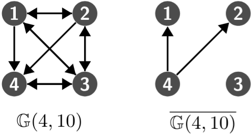
Figure 3: Example illustrating Lemma 7

The condition $m\geq(n-1)^{2}$ ensures $n(n-1)-m\leq n$. In the special case when $m=n(n-1)$, the directed star reduces to an isolated vertex, which is consistent with the fact that the complement of a complete graph is an empty graph. Figure 3 provides a simple example to illustrate Lemma 7. Note that $\mathbb{G}(4,10)$, as shown in the figure, is unique. Indeed, Lemma 7 immediately implies that if $(n-1)^{2}\leq m\leq n(n-1)$, then $\mathbb{G}(n,m)$ is unique regardless of which directed tree $\mathbb{G}(n,n-1)$ is. Figure 4 provides two sequences of $\mathbb{G}(n,m)$ graphs for $n=4$ and $3\leq m\leq 10$, inductively constructed by Algorithm 1. The two sequences start from different directed trees, and from $m=9$ onward, the constructed graphs become identical. Graphs with $m=11$ and $m=12$ are omitted to save some space. Note that the uniqueness of $\mathbb{G}(4,9)$, $\mathbb{G}(4,10)$, and $\mathbb{G}(4,11)$ can also be implied by Proposition 1 and Lemma 4.

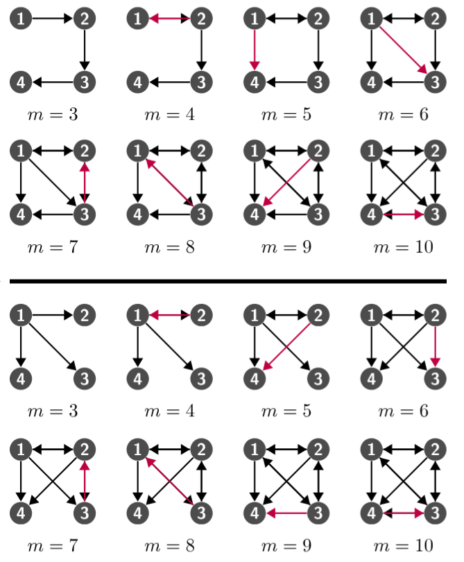
Figure 4: Two sequences of graphs with $n=4$, constructed by Algorithm 1 starting from different directed trees

To prove Lemma 7, we need the following result.

Lemma 8

If there exists an index $k\in\{1,\ldots,n-1\}$ such that $(n,k)$ is an arc in $\mathbb{G}(n,m)$, then the in-degree of vertex $k$ in $\mathbb{G}(n,m)$ is $n-1$.

Proof of Lemma 8: Note that $(n,k)$ cannot be an arc in $\mathbb{G}(n,n-1)$ because any arc in $\mathbb{G}(n,n-1)$ is required to have a head index greater than the tail index. Since the arc $(n,k)$ is not in $\mathbb{G}(n,n-1)$ but is in $\mathbb{G}(n,m)$, from the algorithm description, there must exist exactly one index $p\in\{n,\ldots,m\}$ such that $u_{n,p}=n$ and $v_{n,p}=k$. The algorithm sets $u_{n,p}$ as the smallest vertex index for which $u_{n,p}\neq k$ and $(u_{n,p},k)$ is not an arc in $\mathbb{G}(n,p-1)$. Thus, $(i,k)$ is an arc in $\mathbb{G}(n,p-1)$ for all $i\in\{1,\ldots,n-1\}\setminus\{k\}$. This implies that the in-degree of vertex $k$ in $\mathbb{G}(n,p-1)$ is $n-1$, and the same holds for $\mathbb{G}(n,m)$.  

Proof of Lemma 7: In the special case when $m=n(n-1)$, $\mathbb{G}(n,m)$ is the complete graph, which is the complement of the empty graph. It is easy to verify that the lemma is true in this case. Next consider the case when $(n-1)^{2}\leq m<n(n-1)$ for which $\nu=\lfloor\frac{m}{n}\rfloor=n-2$. From Proposition 1, the vertex in-degree sequence of $\mathbb{G}(n,m)$ is

$$(d_{1},\ldots,d_{n})=(\;\underbrace{n-2,\ldots,n-2}_{n(n-1)-m},\;\underbrace{n-1,\ldots,n-1}_{m-n(n-2)}\;).$$

Since $m\geq(n-1)^{2}$, $m-n(n-2)\geq 1$, which implies that the in-degree of vertex $n$ is $n-1$. Consequently, in $\overline{\mathbb{G}(n,m)}$, the complement of $\mathbb{G}(n,m)$, vertices from $1$ to $(n(n-1)-m)$ have an in-degree of $1$, and the remaining vertices, including vertex $n$, have an in-degree of $0$. Note that the total number of arcs in $\overline{\mathbb{G}(n,m)}$ is $(n(n-1)-m)$. We claim that these $(n(n-1)-m)$ arcs form a directed star rooted at vertex $n$, with leaf vertices labeled from $1$ to $(n(n-1)-m)$, which immediately implies the lemma. To prove the claim, it is equivalent to show that $(n,k)$ is an arc in $\overline{\mathbb{G}(n,m)}$ for all $k\in\{1,\ldots,n(n-1)-m\}$. To this end, suppose to the contrary that $(n,k)$ is not an arc in $\overline{\mathbb{G}(n,m)}$ for some $k\in\{1,\ldots,n(n-1)-m\}$. This implies that $(n,k)$ is an arc in $\mathbb{G}(n,m)$. From Lemma 8, the in-degree of vertex $k$ in $\mathbb{G}(n,m)$ is $n-1$. But this contradicts the fact that $d_{k}=n-2$. Therefore, the claim is true.  

Let $L(n,m)$ denote the Laplacian matrix of $\mathbb{G}(n,m)$, with its $ij$th entry denoted by $[L(n,m)]_{ij}$. It has the following entry-wise property.

Lemma 9

For any integers $n$ and $m$ such that $n\geq 2$ and $n-1\leq m\leq(n-1)^{2}$, $[L(n,m)]_{in}=0$ for each $i\in\{1,\ldots,n-1\}$.

Proof of Lemma 9: The lemma is clearly true when $n=2$. We thus focus on $n\geq 3$. To prove the lemma, suppose to the contrary that $[L(n,m)]_{in}\neq 0$ for some $i\in\{1,\ldots,n-1\}$. From the definition of a Laplacian matrix, the off-diagonal entry $[L(n,m)]_{in}=-1$, which implies that $(n,i)$ is an arc in $\mathbb{G}(n,m)$. From Lemma 8, the in-degree of vertex $i$ in $\mathbb{G}(n,m)$, denoted as $d_{i}$, is $n-1$. We now consider three cases for the value of $m$. First suppose $m=(n-1)^{2}$, which implies $\nu=\lfloor\frac{m}{n}\rfloor=n-2$. From Proposition 1, vertex $n$ has an in-degree of $n-1$, and all other vertices have an in-degree of $n-2$. This contradicts $d_{i}=n-1$. Next suppose $m=n(n-2)$, which implies $\nu=n-2$. It follows from Proposition 1 that all vertices have an in-degree of $n-2$, which contradicts $d_{i}=n-1$. Last suppose $m<n(n-2)$, which implies $\nu\leq\frac{m}{n}<n-2$. From Proposition 1, the maximum in-degree of $\mathbb{G}(n,m)$ is at most $\nu+1$, which is smaller than $n-1$. But this is impossible because $d_{i}=n-1$. Therefore, no matter the value of $m$, a contradiction always occurs, proving that $[L(n,m)]_{in}=0$ for all $i\in\{1,\ldots,n-1\}$.  

Lemma 9 has the following important implication. Recall that Algorithm 1 may generate different graph sequences depending on the initial tree graph.

Lemma 10

Let $\mathbb{G}(n,m)$ be the graph constructed by Algorithm 1 starting from a directed tree $\mathbb{G}(n,n-1)$. If $n\geq 3$ and $n-1\leq m\leq(n-1)^{2}$, then the subgraph of $\mathbb{G}(n,m)$ induced by the vertex subset $\{1,\ldots,n-1\}$ is $\mathbb{G}(n-1,m-d_{n})$, the graph constructed by Algorithm 1 starting from the subgraph of $\mathbb{G}(n,n-1)$ induced by the vertex subset $\{1,\ldots,n-1\}$, where $d_{n}$ is the in-degree of vertex $n$ in $\mathbb{G}(n,m)$.

Since $\mathbb{G}(n,n-1)$ is an $n$-vertex directed tree with vertex $n$ as a leaf, its subgraph induced by the vertex subset $\{1,\ldots,n-1\}$ is a directed tree with $n-1$ vertices. The subgraph also satisfies the requirement that every arc has a head index greater than the tail index, so it can serve as an initial tree graph $\mathbb{G}(n-1,n-2)$ for Algorithm 1 to construct graphs with $n-1$ vertices. In addition, recall that $\mathbb{G}(n,n-1)$ is rooted at vertex $1$, and so is $\mathbb{G}(n,m)$ for any $m\in\{n,\ldots,n(n-1)\}$. Then, the subgraph of $\mathbb{G}(n,m)$ induced by the vertex subset $\{1,\ldots,n-1\}$ is also rooted at vertex $1$ and therefore has at least $n-2$ arcs. Since $m-d_{n}$ is an upper bound on the total number of arcs in the subgraph, its value is no smaller than $n-2$. In the following proof, we will soon show that $m-d_{n}\leq(n-1)(n-2)$. These two facts guarantee that $\mathbb{G}(n-1,m-d_{n})$ is well-defined.

Proof of Lemma 10: Let $\mathbb{H}$ be the subgraph of $\mathbb{G}(n,m)$ induced by the vertex subset $\{1,\ldots,n-1\}$. From Lemma 9, vertex $n$ has no outgoing arcs in $\mathbb{G}(n,m)$. Then, $\mathbb{H}$ has $n-1$ vertices and $m-d_{n}$ arcs, which implies $m-d_{n}\leq(n-1)(n-2)$. In addition, each vertex $i\in\{1,\ldots,n-1\}$ has the same in-degree $d_{i}$ in $\mathbb{H}$ as in $\mathbb{G}(n,m)$, with the values of $d_{i}$, $i\in\{1,\ldots,n\}$, being given in (4). Let $b_{i}$ denote the in-degree of vertex $i$ in $\mathbb{G}(n-1,m-d_{n})$. From Proposition 1,

$$(b_{1},\ldots,b_{n-1})=(\underbrace{u,\ldots,u,}_{(n-1)(u+1)-(m-d_{n})}\underbrace{u+1,\ldots,u+1}_{(m-d_{n})-(n-1)u}\;\;),$$

where $u=\lfloor\frac{m-d_{n}}{n-1}\!\rfloor$. We claim that $b_{i}=d_{i}$ for all $i\in\{1,\ldots,n-1\}$. To prove the claim, we consider two scenarios separately. First, suppose that $n$ divides $m$. Then, from (4), all $d_{i}$, $i\in\{1,\ldots,n\}$ equal $\nu=\frac{m}{n}$, which implies that $n-1$ divides $m-d_{n}$ and $u=\nu$. It follows that all $b_{i}$, $i\in\{1,\ldots,n-1\}$ equal $u$, and thus the claim holds. Next, suppose that $n$ does not divide $m$. Then, $d_{n}=\nu+1=\lfloor\frac{m}{n}\rfloor+1$ and $m=\nu n+r$, where $1\leq r\leq n-1$ is the unique remainder when $m$ is divided by $n$. With these, $u=\lfloor\frac{m-d_{n}}{n-1}\!\rfloor=\lfloor\frac{\nu n+r-\nu-1}{n-1}\rfloor=\nu+\lfloor\frac{r-1}{n-1}\rfloor=\nu$ and thus $(n-1)(u+1)-(m-d_{n})=n(\nu+1)-m$, which validates the claim. This ensures that for each $i\in\{1,\ldots,n-1\}$, vertex $i$ has an in-degree of $d_{i}$ in both $\mathbb{H}$ and $\mathbb{G}(n-1,m-d_{n})$. Since $\mathbb{G}(n-1,n-2)$ is the subgraph of $\mathbb{G}(n,n-1)$ induced by the vertex subset $\{1,\ldots,n-1\}$, where the former is a directed tree with $n-1$ vertices and the latter is a directed tree with $n$ vertices, for each $i\in\{1,\ldots,n-1\}$, vertex $i$ has the same unique in-neighbor index in both trees. With this, Lemma 4 implies that each vertex has the same set of in-neighbor indices in $\mathbb{H}$ and $\mathbb{G}(n-1,m-d_{n})$. Therefore, $\mathbb{H}=\mathbb{G}(n-1,m-d_{n})$.  

We will also need the following lemmas regarding the relationship between $\kappa=\lfloor\frac{m}{n-1}\rfloor$ and $\nu=\lfloor\frac{m}{n}\rfloor$.

Lemma 11

$\nu\in\{\kappa-1,\kappa\}$ for any integers $n$ and $m$ such that $n\geq 2$ and $1\leq m\leq n(n-1)$.

Proof of Lemma 11: Since $\lfloor\frac{m}{n-1}\rfloor\leq\frac{m}{n-1}$ and $\lfloor\frac{m}{n}\rfloor>\frac{m}{n}-1$, it follows that $\kappa-\nu=\lfloor\frac{m}{n-1}\rfloor-\lfloor\frac{m}{n}\rfloor<\frac{m}{n-1}-(\frac{m}{n}-1)=\frac{m}{n(n-1)}+1\leq 2$. As $\kappa-\nu$ is a nonnegative integer, it can only take a value of either 0 or 1, which implies that $\nu$ is equal to either $\kappa$ or $\kappa-1$.  

Lemma 12

$\lfloor\frac{m-\nu-1}{n-2}\rfloor=\kappa$ for any integers $n$ and $m$ such that $n\geq 3$ and $1\leq m\leq n(n-2)$.

Proof of Lemma 12: First, consider the special case when $1\leq m\leq n-2$, which implies $\kappa=\nu=0$. Then, $\lfloor\frac{m-\nu-1}{n-2}\rfloor=\lfloor\frac{m-1}{n-2}\rfloor=0=\kappa$. Thus, the lemma holds in this case.

Next, consider the general case when $n-1\leq m\leq n(n-2)$. Note that $m$ can be written as $m=\kappa(n-1)+r$, where $0\leq r\leq n-2$ is the unique remainder when $m$ is divided by $n-1$. From Lemma 11, $\nu$ equals either $\kappa$ or $\kappa-1$. Let us first suppose $\nu=\kappa$. Then, $\frac{\kappa(n-1)+r}{n}=\frac{m}{n}\geq\lfloor\frac{m}{n}\rfloor=\nu=\kappa$, which implies $r\geq\kappa=\lfloor\frac{m}{n-1}\rfloor\geq 1$. Thus, $\lfloor\frac{m-\nu-1}{n-2}\rfloor=\lfloor\frac{\kappa(n-1)+r-\kappa-1}{n-2}\rfloor=\kappa+\lfloor\frac{r-1}{n-2}\rfloor=\kappa$. In the next step, we suppose $\nu=\kappa-1$. Then, $\lfloor\frac{m-\nu-1}{n-2}\rfloor=\lfloor\frac{\kappa(n-1)+r-\kappa}{n-2}\rfloor=\kappa+\lfloor\frac{r}{n-2}\rfloor$, which equals $\kappa$ if $0\leq r<n-2$. To complete the proof, it remains to consider the case when $r=n-2$. We claim that $r\neq n-2$. To prove the claim, suppose to the contrary that $r=n-2$, with which $m=\kappa(n-1)+r=\kappa n+(n-2-\kappa)$. Meanwhile, as $n\geq 3$ and $1\leq m\leq n(n-2)$, $\kappa=\lfloor\frac{m}{n-1}\rfloor\leq\frac{n(n-2)}{n-1}<n-1$, which implies that $n-1-\kappa$ is a positive integer. Then, $n-2-\kappa\geq 0$, and thus $\nu=\lfloor\frac{m}{n}\rfloor=\lfloor\frac{\kappa n+(n-2-\kappa)}{n}\rfloor=\kappa+\lfloor\frac{n-2-\kappa}{n}\rfloor=\kappa$. But this contradicts $\nu=\kappa-1$. Therefore, $r\neq n-2$.  

Lemma 13

For any integers $n$ and $m$ such that $n\geq 3$ and $1\leq m<n(n-2)$, if $n$ divides $m$, then $\kappa=\nu=\lfloor\frac{m-\nu}{n-2}\rfloor$.

Proof of Lemma 13: Since $n$ divides $m$, $m=\nu n$. Then, $\kappa=\lfloor\frac{m}{n-1}\rfloor=\lfloor\frac{\nu n}{n-1}\rfloor=\lfloor\nu+\frac{\nu}{n-1}\rfloor=\nu+\lfloor\frac{\nu}{n-1}\rfloor=\nu$. Note that $\nu=\frac{m}{n}<n-2$. Therefore, $\lfloor\frac{m-\nu}{n-2}\rfloor=\lfloor\frac{n\nu-\nu}{n-2}\rfloor=\lfloor\nu+\frac{\nu}{n-2}\rfloor=\nu+\lfloor\frac{\nu}{n-2}\rfloor=\nu=\kappa$.  

We are now in a position to prove Theorem 1.

Proof of Theorem 1: We will prove the following claim.

Claim: For any $n\geq 2$ and $n-1\leq m\leq n(n-1)$,

$$p_{L(n,m)}(\lambda)=\lambda(\lambda-\kappa)^{(\kappa+1)(n-1)-m}(\lambda-\kappa-1)^{m-\kappa(n-1)}.$$

Recall that for each pair of $n$ and $m$, distinct $\mathbb{G}(n,m)$ may be generated by Algorithm 1, depending on the choice of the initial tree $\mathbb{G}(n,n-1)$. It is worth emphasizing that we will show the claim holds for all possible $\mathbb{G}(n,m)$, that is, the above characteristic polynomial equation is satisfied for all possible $L(n,m)$.

Note that $1+[(\kappa+1)(n-1)-m]+[m-\kappa(n-1)]=n$. The claim implies that $L(n,m)$ has one eigenvalue at 0, $(\kappa+1)(n-1)-m$ eigenvalues at $\kappa$, and $(\kappa+1)(n-1)-m$ at $\kappa+1$, which together constitute the entire spectrum of $L(n,m)$. The theorem then immediately follows from the claim. Thus, to prove the theorem, it is sufficient to establish the claim. We will prove the claim by induction on $n$.

In the base case when $n=2$, all possible values of $m$ are $1$ and $2$. According to the algorithm description, $\mathbb{G}(2,1)$ contains one arc, $(1,2)$, and $\mathbb{G}(2,2)$ contains two arcs, $(1,2)$ and $(2,1)$. It is straightforward to verify that the claim holds for both $L(2,1)$ and $L(2,2)$. Note that in this special case, $\mathbb{G}(2,1)$ is unique, and so is $\mathbb{G}(2,2)$.

For the inductive step, suppose that the claim holds for $n=q$ for all possible values of $m$ in $\{q-1,\ldots,q(q-1)\}$ and all possible $\mathbb{G}(q,q-1)$, where $q\geq 2$ is an integer. Let $n=q+1$. Take into account all possible $\mathbb{G}(q+1,q)$ and the corresponding values of $m$, which range from $q$ to $(q+1)q$.

We first consider the case when $m\in\{q,\ldots,q^{2}-1\}$. From Lemma 9, with $n$ replaced by $q+1$, $[L(q+1,m)]_{i(q+1)}=0$ for all $i\in\{1,\ldots,q\}$. That is, all entries in the $(q+1)$th column of $L(q+1,m)$, except for the last entry $[L(q+1,m)]_{(q+1)(q+1)}$, are zero. The same holds for the $(q+1)$th column of $\lambda I-L(q+1,m)$, whose last entry is equal to $\lambda-[L(q+1,m)]_{(q+1)(q+1)}$. Then, the Laplace expansion along the $n$th column of $L(q+1,m)$ yields

$$p_{L(q+1,m)}(\lambda) =\det\big{(}\lambda I-L(q+1,m)\big{)}$$

$$=\big{(}\lambda-[L(q+1,m)]_{(q+1)(q+1)}\big{)}p_{M}(\lambda),$$ (7)

where $M$ is the $q\times q$ submatrix of $L(q+1,m)$ obtained by removing the $(q+1)$th row and $(q+1)$th column of $L(q+1,m)$. Since all row sums of $L(q+1,m)$ are zero, and all entries in its $(q+1)$th column, except for the last entry, are zero, $M$ also has all row sums equal to zero. It follows that $M$ is the Laplacian matrix of a certain graph $\mathbb{H}$ with $q$ vertices, and $\mathbb{H}$ is the subgraph of $\mathbb{G}(q+1,m)$ induced by the vertex subset $\{1,\ldots,q\}$. From Lemma 10, with $n$ replaced by $q+1$, $\mathbb{H}=\mathbb{G}(q,m-d_{q+1})$, where $d_{q+1}$ denotes the in-degree of vertex $q+1$ in $\mathbb{G}(q+1,m)$, and $\mathbb{G}(q,m-d_{q+1})$ is the graph constructed by Algorithm 1 starting from the subgraph of $\mathbb{G}(q+1,q)$ induced by the vertex subset $\{1,\ldots,q\}$. Thus, $M$ is the Laplacian matrix of $\mathbb{G}(q,m-d_{q+1})$. Let $\gamma\stackrel{{\scriptstyle\Delta}}{{=}}\lfloor\frac{m}{q+1}\rfloor$. We consider the following two cases separately.

Case 1: Suppose that $q+1$ divides $m$, which implies $m=\gamma(q+1)$. From the definition of a Laplacian matrix and Proposition 1, $[L(q+1,m)]_{(q+1)(q+1)}=d_{q+1}=\gamma$. Then, $M$ is the Laplacian matrix of $\mathbb{G}(q,m-d_{q+1})=\mathbb{G}(q,m-\gamma)$. From (7) and the induction hypothesis,

$$p_{L(q+1,m)}(\lambda)=(\lambda-\gamma)p_{M}(\lambda),$$ (8)

$$p_{M}(\lambda)=\lambda(\lambda-\beta)^{(\beta+1)(q-1)-m+\gamma}(\lambda-\beta-1)^{m-\gamma-\beta(q-1)},$$

where $\beta\stackrel{{\scriptstyle\Delta}}{{=}}\lfloor\frac{m-\gamma}{q-1}\rfloor$. The analysis is further divided into two scenarios based on the value of $m$. First, consider when $m=q^{2}-1$, which implies $\gamma=q-1$ and thus $\beta=q$. Then, $(\beta+1)(q-1)-m+\gamma=q-1$ and $m-\gamma-\beta(q-1)=0$. It follows from (8) that

$$p_{L(q+1,m)}(\lambda)=\lambda(\lambda-q+1)(\lambda-1)^{q-1}.$$

Meanwhile, $(\gamma+1)q-m=1$ and $m-\gamma q=q-1$. Thus, the above equation validates the claim with $n$ replaced by $q+1$. Next, consider when $1\leq m\leq q^{2}-2$. From Lemma 13, with $n$ replaced by $q+1$, $\gamma=\beta=\alpha\stackrel{{\scriptstyle\Delta}}{{=}}\lfloor\frac{m}{q}\rfloor$. Then, from (8),

$$p_{L(q+1,m)}(\lambda)=\lambda(\lambda-\alpha)^{(\alpha+1)q-m}(\lambda-\alpha-1)^{m-\alpha q},$$ (9)

which proves the claim with $n$ replaced by $q+1$.

Case 2: Suppose that $q+1$ does not divide $m$, which implies $m-\gamma(q+1)>0$. From the definition of a Laplacian matrix and Proposition 1, $[L(q+1,m)]_{(q+1)(q+1)}=d_{q+1}=\gamma+1$. Then, $M$ is the Laplacian matrix of $\mathbb{G}(q,m-d_{q+1})=\mathbb{G}(q,m-\gamma-1)$. From (7) and the induction hypothesis,

$$p_{L(q+1,m)}(\lambda)=(\lambda-\gamma-1)p_{M}(\lambda),$$ (10)

$$p_{M}(\lambda)\!=\!\lambda(\lambda-\beta^{\prime})^{(\beta^{\prime}+1)(q-1)-m+\gamma^{\prime}}(\lambda-\beta^{\prime}-1)^{m-\gamma^{\prime}-\beta^{\prime}(q-1)},$$

where $\gamma^{\prime}=\gamma+1$ and $\beta^{\prime}\stackrel{{\scriptstyle\Delta}}{{=}}\lfloor\frac{m-\gamma-1}{q-1}\rfloor$. With $n$ replaced by $q+1$, Lemma 12 and Lemma 11 respectively imply that $\beta^{\prime}=\alpha$ and $\gamma\in\{\alpha-1,\alpha\}$. The analysis is then divided into two scenarios based on the value of $\gamma$. First, suppose $\gamma=\alpha-1$. Then, $(\beta^{\prime}+1)(q-1)-m+\gamma^{\prime}=(\alpha+1)(q-1)-m+\alpha$ and $m-\gamma^{\prime}-\beta^{\prime}(q-1)=m-\alpha q$. It follows that (10) simplifies to (9), which validates the claim. Next, suppose $\gamma=\alpha$. Then, $(\beta^{\prime}+1)(q-1)-m+\gamma^{\prime}=(\alpha+1)q-m$ and $m-\gamma^{\prime}-\beta^{\prime}(q-1)=m-\alpha q-1$. With these equalities, (10) once again leads to (9), thereby proving the claim.

The two cases above collectively establish the inductive step for $m\in\{q,\ldots,q^{2}-1\}$. In what follows, we address the remaining case where $m\in\{q^{2},\ldots,q^{2}+q\}$. From Lemma 7, with $n$ replaced by $q+1$, $\overline{\mathbb{G}(q+1,m)}$, the complement of $\mathbb{G}(q+1,m)$, is the $(q+1)$-vertex directed forest consisting of a directed star with $(q^{2}+q-m+1)$ vertices, rooted at vertex $q+1$, and $m-q^{2}$ isolated vertices. Thus, $\overline{\mathbb{G}(q+1,m)}$ is acyclic, with $(q^{2}+q-m)$ vertices of in-degree $1$ and the other $(m-q^{2}+1)$ vertices of in-degree $0$. From Lemma 5, the Laplacian spectrum of $\overline{\mathbb{G}(q+1,m)}$ consists of $(q^{2}+q-m)$ eigenvalues at $1$ and $(m-q^{2}+1)$ eigenvalues at $0$. Then, from Lemma 6, the Laplacian spectrum of $\mathbb{G}(q+1,m)$ is composed of a single eigenvalue of $0$, an eigenvalue of $q$ with multiplicity $q^{2}+q-m$, and an eigenvalue of $q+1$ with multiplicity $m-q^{2}$. This leads to

$$p_{L(q+1,m)}(\lambda)=\lambda(\lambda-q)^{q^{2}+q-m}(\lambda-q-1)^{m-q^{2}},$$

which validates the claim with $n$ replaced by $q+1$. We therefore complete the proof of the inductive step.  

III Proof of the Conjecture for Special Cases

Theorem 1 establishes that the conjectured Laplacian spectrum (3), and consequently the minimum possible value of $\sigma^{2}$, is always achievable by a class of almost regular directed graphs when $m\geq n-1$. We will shortly prove that it is also achievable when $m<n-1$. In this section, we further show that the conjectured value of $\sigma^{2}$ in (2) is indeed the minimum in certain special cases.

III-A Case When $m\leq n-1$

For this special case, we first characterize all graphs that possess the conjectured Laplacian spectrum (3).

Proposition 2

A simple directed graph with $n\geq 2$ vertices and $m\leq n-1$ arcs has Laplacian spectrum (3) if, and only if, it is a directed forest.

Note that when $m=n-1$, the proposition implies that the Laplacian spectrum (3) is achieved if and only if the graph is an $n$-vertex directed tree. This is consistent with the implementation of Algorithm 1, in which $\mathbb{G}(n,n-1)$ can be chosen as any directed tree with $n$ vertices.

To prove Proposition 2, we need the following concept and lemma. Let us agree to say that a subgraph of a directed graph $\mathbb{G}$ spans $\mathbb{G}$ if it contains all vertices of $\mathbb{G}$.

Lemma 14

For any simple directed graph $\mathbb{G}$, the algebraic multiplicity of eigenvalue 0 in its Laplacian spectrum equals the minimum number of directed trees in any directed forest that spans $\mathbb{G}$.

Three examples are provided in Figure 5 to illustrate the lemma. The Laplacian matrix of the left graph in Figure 5 has one eigenvalue at 0, and there is one directed tree subgraph that can span the graph, one possible instance of which is depicted in blue. The middle graph in Figure 5 has two eigenvalues at 0 in its Laplacian spectrum, and the minimum number of directed trees in any directed forest that spans the graph is also 2. One such spanning directed forest is depicted in purple and blue, representing its two directed trees, respectively. The right graph in Figure 5 has three eigenvalues equal to 0, and the minimum number of directed trees in any directed forest that spans the graph is also 3. One such spanning forest consists of a directed tree with three vertices depicted in blue, along with two isolated vertices, each considered a trivial tree.

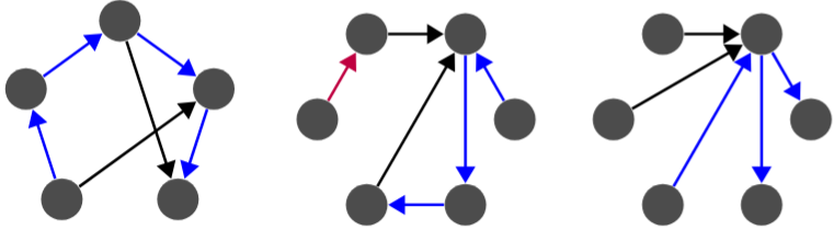
Figure 5: Three examples of spanning directed forests

In the case when the algebraic multiplicity of the eigenvalue $0$ is $1$, Lemma 14 implies that the graph has a spanning directed tree, that is, it is rooted. Therefore, the lemma yields that a simple directed graph has a simple zero Laplacian eigenvalue if and only if it is rooted. A counterpart result was proved in [10, Lemma 2] for out-degree Laplacian matrices.

Lemma 14 is a direct consequence of Corollary 1 in [11], which proves that the algebraic multiplicity of the eigenvalue 0 in the out-degree Laplacian spectrum of a simple directed graph equals the minimum number of “in-trees” in any “in-forest” that spans the graph. The transpose of a directed graph is a directed graph with the same vertex set, but with all arcs reversed in direction compared to the corresponding arcs in the original graph. A directed graph is called an in-tree or in-forest if its transpose is a directed tree or a directed forest, respectively. Three examples illustrating the corollary are presented in Figure 6, which are respectively the transposes of the three graphs in Figure 5.

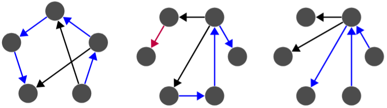
Figure 6: Three examples of spanning in-forests

Return to the statement of Lemma 14. Let $\mathbb{G}^{\prime}$ be the transpose of graph $\mathbb{G}$. It is straightforward to verify that the out-degree based Laplacian matrix (see the definition in the second paragraph of the introduction) of $\mathbb{G}^{\prime}$ is equal to the (in-degree based) Laplacian matrix of $\mathbb{G}$. From Corollary 1 in [11], the algebraic multiplicity of eigenvalue 0 in the out-degree Laplacian spectrum of $\mathbb{G}^{\prime}$ equals the minimum number of in-trees in any in-forest that spans $\mathbb{G}^{\prime}$. Therefore, from the relationship between in-trees and directed trees, as well as between in-forests and directed forests, the algebraic multiplicity of the eigenvalue 0 in the (in-degree) Laplacian spectrum of $\mathbb{G}$ equals the minimum number of directed trees in any directed forest spanning $\mathbb{G}$.

We here provide a more direct proof of Lemma 14 using a generalized version of the well-known Kirchhoff’s matrix tree theorem. To state the generalized matrix tree theorem, we need the following concept.

A weighted simple directed graph is a simple directed graph in which each arc is assigned a nonzero real number as its weight. An unweighted simple directed graph can be viewed as a special case of a weighted graph where all weights are equal to 1. The Laplacian matrix of a weighted simple directed graph is defined as the difference between the weighted in-degree matrix and the adjacency matrix, where the weighted in-degree matrix is a diagonal matrix whose $i$th diagonal entry equals the sum of all in-degree arc weights of vertex $i$, and the adjacency matrix is defined such that its $ij$th entry equals the weight of arc $(j,i)$, or 0 if no such arc exists. This definition of the Laplacian clearly simplifies to the one given in the introduction when the graph is unweighted. The definition implies that any Laplacian matrix has all row sums equal to 0. It is easy to see that any real matrix with all row sums equal to 0 can be interpreted as the Laplacian matrix of a uniquely determined weighted simple directed graph.

For any simple weighted graph $\mathbb{G}$, let $w(\mathbb{G})$ denote the product of the weights of all arcs in $\mathbb{G}$. In the special case when $\mathbb{G}$ has no arcs, $w(\mathbb{G})$ is defined to be 1.

Lemma 15

(second Theorem on page 379 of [12]) Let $M$ be any $n\times n$ real matrix with all row sums equal to zero, and let $\mathbb{G}$ denote the weighted simple directed graph uniquely determined by $M$. For any $1\leq k\leq n$ distinct indices $i_{1},\ldots,i_{k}\in\{1,\ldots,n\}$, the $(n-k)\times(n-k)$ principal minor of $M$ obtained by removing its rows and columns indexed by $i_{1},\ldots,i_{k}$ is equal to $\sum_{\mathbb{F}\in\mathcal{F}}w(\mathbb{F})$, where $\mathcal{F}$ is the set of spanning directed forests of $\mathbb{G}$ composed of $k$ directed trees rooted at vertices $i_{1},\ldots,i_{k}$.

In the special case when $k=n$, there is only one spanning directed forest composed of $k$ directed trees rooted at $k$ distinct indices; this forest is the spanning subgraph of $\mathbb{G}$ without any arcs, consisting of $n$ isolated vertices. Then, $\sum_{\mathbb{F}\in\mathcal{F}}w(\mathbb{F})=1$, which is consistent with the convention that a minor of order zero is defined as 1.

In another special case when all arc weights of $\mathbb{G}$ are equal to 1, each $w(\mathbb{F})$, $\mathbb{F}\in{\cal F}$ equals 1, and thus $\sum_{\mathbb{F}\in\mathcal{F}}w(\mathbb{F})$ simplifies to the number of spanning directed forests in ${\cal F}$. This leads to the following corollary.

Corollary 1

Let $L$ be the Laplacian matrix of a simple directed graph $\mathbb{G}$ with $n$ vertices. For any $1\leq k\leq n$ distinct indices $i_{1},\ldots,i_{k}\in\{1,\ldots,n\}$, the $(n-k)\times(n-k)$ principal minor of $L$ obtained by removing its rows and columns indexed by $i_{1},\ldots,i_{k}$ is equal to the number of spanning directed forests of $\mathbb{G}$ composed of $k$ directed trees rooted at vertices $i_{1},\ldots,i_{k}$.

We can now provide a simple proof of Lemma 14.

Proof of Lemma 14: Write the characteristic polynomial of $L$ as $p(\lambda)=\det(\lambda I-L)$. It is well known that $p(\lambda)=\sum_{k=0}^{n}(-1)^{n-k}a_{k}\lambda^{k}$, where $a_{k}$ is the sum of all principal minors of $L$ of order $n-k$. In particular, $a_{0}=\det(L)=0$ because $L$ has an eigenvalue at 0. From Corollary 1, $a_{k}$ equals the total number of spanning directed forests of $\mathbb{G}$ consisting of exactly $k$ directed trees. Let $q$ denote the minimum number of directed trees in any spanning directed forest of $\mathbb{G}$. Then, $a_{k}=0$ for all $k\in\{1,\ldots,q-1\}$, and $a_{k}>0$ for all $k\in\{q,\ldots,n\}$. From the preceding discussion, $p(\lambda)=\sum_{k=q}^{n}(-1)^{n-k}a_{k}\lambda^{k}=\lambda^{q}\sum_{k=q}^{n}(-1)^{n-k}a_{k}\lambda^{k-q}$, which implies that the algebraic multiplicity of eigenvalue 0 is equal to $q$.  

With Lemma 14, we are ready to prove Proposition 2.

Proof of Proposition 2: We first prove the necessity of the proposition. Suppose the Laplacian spectrum is (3). If $m=n-1$, then $\kappa=\lfloor\frac{m}{n-1}\rfloor=1$, and thus $0$ is a simple eigenvalue. If $m<n-1$, then $\kappa=0$, and the Laplacian spectrum has $n-m$ eigenvalues at $0$. Combining the two cases, the algebraic multiplicity of the eigenvalue $0$ is $n-m$. From Lemma 14, the minimum number of directed trees in any spanning directed forest of the graph is $n-m$. Let $\mathbb{F}$ be such a spanning directed forest, which must exist and consists of $n-m$ directed trees. Without loss of generality, label the directed trees in $\mathbb{F}$ from $1$ to $n-m$. Let $n_{i}$ denote the number of vertices in the $i$th directed tree. Then, $\sum_{i=1}^{n-m}n_{i}=n$, and the total number of arcs in $\mathbb{F}$ is $\sum_{i=1}^{n-m}(n_{i}-1)=n-(n-m)=m$. Since $\mathbb{F}$ is a spanning subgraph and the graph has exactly $m$ arcs, the graph must be equal to the directed forest $\mathbb{F}$.

We next prove the sufficiency of the proposition. Suppose the graph is any directed forest with $n$ vertices and $m$ arcs. Then, $m$ vertices have in-degree $1$, and the remaining $n-m$ vertices have in-degree $0$. From Lemma 5, its Laplacian spectrum consists of $m$ eigenvalues at 1 and $n-m$ eigenvalues at 0. Recall that $\kappa$ equals $1$ when $m=n-1$ and $0$ when $m<n-1$. It is straightforward to verify that the Laplacian spectrum always satisfies (3) for $m\leq n-1$.  

With the Laplacian spectrum (3), the normalized spread of the eigenvalues $\sigma^{2}$ equals $0$ when $m=n-1$ and $m(n-1-m)/(n-1)^{2}$ when $0\leq m<n-1$. It is easy to see that in both cases $\sigma^{2}=m(n-1-m)/(n-1)^{2}$. The following theorem shows this is the minimum possible value of $\sigma^{2}$, which proves the conjecture for $m\leq n-1$.

Theorem 2

Among all simple directed graphs with $n\geq 2$ vertices and $m\leq n-1$ arcs, $\sigma^{2}_{\min}=m(n-1-m)/(n-1)^{2}$, which is achieved if, and only if, the Laplacian spectrum equals (3).

To prove the theorem, we need the following lemmas.

Lemma 16

For any simple directed graph with $n$ vertices and $m$ arcs, $\sigma^{2}=\frac{1}{n-1}\sum_{i=1}^{n}|\lambda_{i}|^{2}-(\frac{m}{n-1})^{2}$, where $\lambda_{1},\ldots,\lambda_{n}$ are the Laplacian eigenvalues of the graph.

Proof of Lemma 16: Since any Laplacian matrix has an eigenvalue at $0$, set $\lambda_{1}=0$ without loss of generality. Recall that $\sigma^{2}=\frac{1}{n-1}\sum_{i=2}^{n}|\lambda_{i}-\bar{\lambda}|^{2}$, where $\bar{\lambda}=\frac{1}{n-1}\sum_{i=2}^{n}\lambda_{i}$. Since the sum of the out-degrees of all $n$ vertices is $m$, and the sum of all eigenvalues of a matrix equals the trace of the matrix, it follows that $\bar{\lambda}=m/(n-1)$, which is always a real number. As complex Laplacian eigenvalues, if any, appear in conjugate pairs, $\sum_{i=2}^{n}(\lambda_{i}+\lambda_{i}^{*})=2\sum_{i=2}^{n}{\rm Re}(\lambda_{i})=2\sum_{i=2}^{n}\lambda_{i}=2m$. Then,

$$\sigma^{2} =\frac{1}{n-1}\sum_{i=2}^{n}|\lambda_{i}-\bar{\lambda}|^{2}=\frac{1}{n-1}\sum_{i=2}^{n}(\lambda_{i}-\bar{\lambda})(\lambda_{i}^{*}-\bar{\lambda})$$

$$=\frac{1}{n-1}\Big{(}\sum_{i=2}^{n}|\lambda_{i}|^{2}-\frac{m}{n-1}\sum_{i=2}^{n}(\lambda_{i}+\lambda_{i}^{*})\Big{)}+\Big{(}\frac{m}{n-1}\Big{)}^{2}$$

$$=\frac{1}{n-1}\sum_{i=2}^{n}|\lambda_{i}|^{2}-\Big{(}\frac{m}{n-1}\Big{)}^{2},$$

which completes the proof.  

Lemma 17

For any simple directed graph with $n$ vertices and $m\leq n-1$ arcs, $\sum_{i=1}^{n}|\lambda_{i}|^{2}\geq m$, with equality if and only if the Laplacian spectrum is (3)

To prove the lemma, we need the following result.

Lemma 18

(Proposition 1.2.11 in [13]) Any simple undirected graph with $n$ vertices and $m$ edges has at least $\max\{n-m,1\}$ connected components.

Proof of Lemma 17: For any simple directed graph $\mathbb{G}$ with $n$ vertices and $m\leq n-1$ arcs, without loss of generality, assume its Laplacian spectrum has $k$ eigenvalues at $0$, and set $\lambda_{1}=\cdots=\lambda_{k}=0$, with the remaining $\lambda_{k+1},\ldots,\lambda_{n}$ nonzero. Since the total out-degree is $m$ and the eigenvalue sum equals the trace, $\sum_{i=k+1}^{n}\lambda_{i}=m$. Note that in the special case when $k=n$, $m=0$ and then the lemma is clearly true. Thus, we consider $k<n$ in the remainder of the proof. By the Cauchy-Schwarz inequality, $(\sum_{i=k+1}^{n}|\lambda_{i}|)^{2}\leq(n-k)(\sum_{i=k+1}^{n}|\lambda_{i}|^{2})$, with equality if and only if $|\lambda_{k+1}|=\cdots=|\lambda_{n}|$. Then,

$$\textstyle\sum_{i=k+1}^{n}|\lambda_{i}|^{2} \overset{(a)}{\geq}\textstyle\frac{1}{n-k}(\sum_{i=k+1}^{n}|\lambda_{i}|)^{2}$$

$$\overset{(b)}{\geq}\textstyle\frac{1}{n-k}|\sum_{i=k+1}^{n}\lambda_{i}|^{2}=\frac{m^{2}}{n-k}.$$

Let $\mathbb{H}$ be the underlying simple undirected graph of $\mathbb{G}$, obtained by replacing all directed edges in $\mathbb{G}$ with undirected ones. Then, $\mathbb{H}$ has at most $m$ undirected edges. With this fact and from Lemma 18, $\mathbb{H}$ has at least $n-m$ connected components. Consequently, $\mathbb{G}$ has at least $n-m$ weakly connected components. To span a weakly connected component, at least one directed tree is required. Thus, the minimum number of directed trees required to form a directed forest that spans $\mathbb{G}$ is at least $n-m$. From Lemma 14, the minimum number of directed trees in any spanning directed forest of $\mathbb{G}$ equals $k$. It follows that $k\geq n-m$, which implies $n-k\leq m$. With this inequality, the preceding discussion leads to $\sum_{i=1}^{n}|\lambda_{i}|^{2}=\sum_{i=k+1}^{n}|\lambda_{i}|^{2}\geq\frac{m^{2}}{n-k}\geq m$.

Moreover, $\sum_{i=1}^{n}|\lambda_{i}|^{2}=m$ if and only if three equalities, namely $(a)$, $(b)$, and $k=n-m$, hold simultaneously. First, recall that equality in $(a)$ holds if and only if $\lambda_{k+1},\ldots,\lambda_{n}$ have the same magnitude. Second, equality in $(b)$ holds if and only if $\lambda_{k+1},\ldots,\lambda_{n}$ have the same phase. These two conditions together imply $\lambda_{k+1}=\cdots=\lambda_{n}$. Last, since $m=n-k>0$, with $\sum_{i=k+1}^{n}\lambda_{i}=m$, $\lambda_{k+1}=\cdots=\lambda_{n}=1$. Therefore, the three equalities hold if and only if the Laplacian spectrum consists of $n-m$ eigenvalues at $0$ and $m$ eigenvalues at $1$. Recall that $\kappa$ equals $1$ when $m=n-1$ and $0$ when $m<n-1$. In both cases, it is straightforward to verify that the Laplacian spectrum (3) contains exactly $n-m$ zeros and $m$ ones. This completes the proof.  

Theorem 2 follows directly from Lemmas 16 and 17.

Proof of Theorem 2: From Lemmas 16 and 17, $\sigma^{2}=\frac{1}{n-1}\sum_{i=1}^{n}|\lambda_{i}|^{2}-(\frac{m}{n-1})^{2}\geq\frac{m}{n-1}-(\frac{m}{n-1})^{2}=m(n-1-m)/(n-1)^{2}$, with equality if and only if the Laplacian spectrum is (3).  

Theorem 2 and Proposition 2 yield the following result.

Corollary 2

Among all simple directed graphs with $n\geq 2$ vertices and $m\leq n-1$ arcs, the minimum normalized spread of the Laplacian eigenvalues is achieved if, and only if, the graph is a directed forest.

The case $m<n-1$ may be less relevant for network synchronization, as the graphs are disconnected. As discussed right after Proposition 2, when $m=n-1$, the optimal graphs with minimum $\sigma^{2}$ are all directed trees. In this case, $\sigma^{2}_{\min}=0$, and the same holds when $m$ is a multiple of $n-1$, as shown in the following subsection.

III-B Case When $m$ Is a Multiple of $n-1$

For a simple directed graph with $n$ vertices, the number of arcs $m$ is at most $n(n-1)$. Thus, if $m$ is a multiple of $n-1$, the multiple is at most $n$. While some results in this subsection overlap with those in the previous one for the case $m=n-1$, they are proved using a different approach.

Theorem 3

Among all simple directed graphs with $n\geq 2$ vertices and $m=l(n-1)$ arcs, where $l\in\{1,\ldots,n\}$, $\sigma^{2}_{\min}=0$, which is achieved if, and only if, the Laplacian spectrum equals (3).

Proof of Theorem 3: It is clear that $\sigma^{2}\geq 0$. To prove sufficiency, suppose the Laplacian spectrum is (3). It is easy to see that $\kappa=l$ and $\sigma^{2}=0$. To prove the necessity, suppose $\sigma^{2}=0$. Then, $\lambda_{2}=\cdots=\lambda_{n}=\bar{\lambda}$. From the proof of Lemma 16, $\bar{\lambda}=m/(n-1)=l$. It follows that the Laplacian spectrum is (3).  

From Theorem 1, any $\mathbb{G}(n,l(n-1))$ constructed by Algorithm 1 has the Laplacian spectrum (3), and thus achieves zero normalized Laplacian eigenvalue spread. Recall that when $l=1$, $\mathbb{G}(n,l(n-1))=\mathbb{G}(n,n-1)$ is the starting graph in Algorithm 1, which is a directed tree rooted at vertex $1$. More can be said about the topology of $\mathbb{G}(n,l(n-1))$. We call the union of two or more directed graphs an arc-disjoint union if no two of the graphs share an arc. Note that this is different from the concept of disjoint union defined earlier. In general, $\mathbb{G}(n,l(n-1))$ is an arc-disjoint union of directed trees, as stated in the following lemma.

Lemma 19

For any integers $n\geq 2$ and $l\in\{1,\ldots,n\}$, any $\mathbb{G}(n,l(n-1))$ constructed by Algorithm 1 is the arc-disjoint union of $l$ directed trees with $n$ vertices, rooted at vertices $1,\ldots,l$, respectively.

It is worth emphasizing that not every arc-disjoint union of directed trees has the Laplacian spectrum (3). For example, the graph in Figure 7 is an arc-disjoint union of two directed trees (shown in black and blue), rooted at vertices 1 and 2, respectively. Its Laplacian spectrum is $\{0,2,2,2,2-i,2+i\}$, which does not match (3).

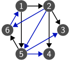
Figure 7: A union of two $6$-vertex directed trees that does not achieve the minimum normalized eigenvalue spread

Lemma 19 follows immediately from the following result.

Lemma 20

For any integers $n\geq 2$ and $l\in\{2,\ldots,n\}$, $\mathbb{G}(n,l(n-1))$ is the arc-disjoint union of $\mathbb{G}(n,(l-1)(n-1))$ and a directed tree rooted at vertex $l$.

Figure 8 illustrates the lemma. The three graphs shown are $\mathbb{G}(6,5)$, $\mathbb{G}(6,10)$, and $\mathbb{G}(6,15)$, taken from Figure 1. The graph $\mathbb{G}(6,10)$ adds a directed tree rooted at vertex $2$ (in blue) to $\mathbb{G}(6,5)$. Similarly, $\mathbb{G}(6,15)$ adds another directed tree rooted at vertex $3$ (in purple) to $\mathbb{G}(6,10)$. The three graphs also illustrate Lemma 19.

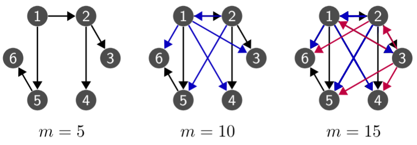
Figure 8: Examples illustrating Lemmas 19 and 20 for $n=6$

Proof of Lemma 20: From the algorithm description, $\mathbb{G}(n,l(n-1))$ is built from $\mathbb{G}(n,(l-1)(n-1))$ by adding $n-1$ arcs. Let $\mathbb{H}$ denote the graph with $n$ vertices consisting of these $n-1$ arcs. The in-degree distribution of $\mathbb{H}$ can thus be obtained by examining the difference in in-degree distributions between $\mathbb{G}(n,l(n-1))$ and $\mathbb{G}(n,(l-1)(n-1))$. From Proposition 1, in $\mathbb{G}(n,l(n-1))$, vertices $1$ to $l$ have an in-degree of $l-1$, and vertices $l+1$ to $n$ have an in-degree of $l$. Similarly, in $\mathbb{G}(n,(l-1)(n-1))$, vertices $1$ to $l-1$ have an in-degree of $l-2$, and vertices $l$ to $n$ have an in-degree of $l-1$. Therefore, all $n$ vertices in $\mathbb{H}$ have an in-degree of $1$, except for vertex $l$ whose in-degree equals $0$. To prove the lemma, it is equivalent to show that $\mathbb{H}$ is a directed tree rooted at vertex $l$; that is, all other vertices are reachable from vertex $l$ in $\mathbb{H}$.

We first consider the vertices in $\{1,\ldots,l-1\}$, whose in-degrees in $\mathbb{G}(n,(l-1)(n-1))$ are all equal to $l-2$. Lemma 4 identifies the in-neighbors of each vertex $i\in\{1,\ldots,l-1\}$ in $\mathbb{G}(n,(l-1)(n-1))$. We claim that the $l-2$ incoming arcs of each vertex $i$ originate from the $l-2$ vertices in $\{1,\ldots,l-1\}\setminus\{i\}$. If $l=2$, then $i$ must be $1$. In the case when $i=1$, the $l-2$ in-neighbors have indices in $\{2,\ldots,l-1\}$. In the case when $l\geq 3$ and $i\in\{2,\ldots,l-1\}$, the indices of the $l-2$ in-neighbors are $i_{j}$, the unique vertex index such that $(i_{j},i)$ is an arc in $\mathbb{G}(n,n-1)$, together with the $l-3$ smallest elements of $\{1,\ldots,n\}\setminus\{i,i_{j}\}$. Since $i_{j}<i\leq l-1$, the set of in-neighbor indices simplifies to $\{1,\ldots,l-1\}\setminus\{i\}$. It can be seen that the claim holds in all cases. From the algorithm description, the single incoming arc of each vertex $i\in\{1,\ldots,l-1\}$ in $\mathbb{H}$ must originate from the smallest index $u$ such that $(u,i)$ is not an arc in $\mathbb{G}(n,(l-1)(n-1))$. Then, $u=l$. That is, $(l,i)$ is an arc in $\mathbb{H}$ for each $i\in\{1,\ldots,l-1\}$.

Next consider any vertex $i\in\{l+1,\ldots,n\}$. Since vertex $i$ has in-degree $l-1$ in $\mathbb{G}(n,(l-1)(n-1))$, there must exist at least one vertex $v\in\{1,\ldots,l\}$ such that $(v,i)$ is not an arc in $\mathbb{G}(n,(l-1)(n-1))$. Without loss of generality, assume $v$ has the smallest index among such vertices. As vertex $i$ has in-degree $1$ in $\mathbb{H}$, it follows from the algorithm description that $(v,i)$ must be the incoming arc to vertex $i$ in $\mathbb{H}$. If $v=l$, then vertex $l$ is an in-neighbor of vertex $i$. If $v\leq l-1$, then, as shown in the previous paragraph, $(l,v)$ is an arc in $\mathbb{H}$, so vertex $i$ is reachable from vertex $l$ along the directed path $(l,v)(v,i)$.

We have shown that $\mathbb{H}$ has $n-1$ arcs and that all its $n$ vertices are reachable from vertex $l$. Therefore, $\mathbb{H}$ must be a directed tree rooted at vertex $l$.  

The necessary and sufficient graphical characterization of optimal graphs with $\sigma^{2}_{\min}=0$, in the case when $m$ is a multiple of $n-1$, has so far eluded us.

III-C Case When $m\geq(n-1)^{2}$

We first characterize all graphs with $m\geq(n-1)^{2}$ whose Laplacian spectrum is given by (3).

Proposition 3

A simple directed graph with $n\geq 2$ vertices and $m\geq(n-1)^{2}$ arcs has Laplacian spectrum (3) if, and only if, its complement is a directed forest.

Figure 9 illustrates the proposition. The graph $\mathbb{G}$ on the left has $6$ vertices and $27$ arcs. Its Laplacian spectrum is $\{4,4,4,5,5,5\}$, which matches (3). The complement of $\mathbb{G}$, shown on the right, is a directed forest, consistent with the statement of the proposition. It is worth noting that this graph $\mathbb{G}$ cannot be generated by Algorithm 1. To see this, Lemma 7 implies the uniqueness of $\mathbb{G}(6,27)$, and states that its complement is a $6$-vertex directed forest consisting of a $4$-vertex directed star and $2$ isolated vertices. Therefore, $\mathbb{G}$ is not $\mathbb{G}(6,27)$. Note that for $m\geq(n-1)^{2}$, Theorem 1 can be implied by Lemma 7 and Proposition 3.

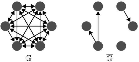
Figure 9: An example illustrating Proposition 3

Proposition 3 is a direct consequence of the following lemma and Proposition 2.

Lemma 21

A simple directed graph has Laplacian spectrum (3) if, and only if, its complement does as well.

It is worth emphasizing that the lemma implies any graph and its complement share the same conjectured formula (2) for the minimal possible normalized Laplacian eigenvalue spread. While their explicit expressions of the formula in terms of $n$ and $m$ may differ (e.g., Theorem 2 vs. Theorem 4) due to the dependence of $\kappa$ on the number of arcs, the resulting values are the same because of the arc count relation between a graph and its complement (cf. Lemma 22).

Proof of Lemma 21: Since the complement of a graph’s complement is the graph itself, to prove the lemma, it is sufficient to show that if a directed graph $\mathbb{G}$, with $n$ vertices and $m$ arcs, has Laplacian spectrum (3), then so does its complement $\overline{\mathbb{G}}$, which has $n$ vertices and $\overline{m}=n(n-1)-m$ arcs. For such a $\mathbb{G}$, it follows from (3) and Lemma 6 that the Laplacian spectrum of $\overline{\mathbb{G}}$ is

$$0,\;\underbrace{n-\kappa-1,\ldots,n-\kappa-1}_{m-(n-1)\kappa},\;\;\underbrace{n-\kappa,\ldots,n-\kappa}_{(n-1)(\kappa+1)-m}.$$ (11)

We claim that (11) matches (3). To prove this, set $\overline{\kappa}=\lfloor\frac{n(n-1)-m}{n-1}\rfloor$ for $\overline{\mathbb{G}}$. First suppose $m$ is a multiple of $n-1$. Then, $\kappa=\lfloor\frac{m}{n-1}\rfloor=\frac{m}{n-1}$ and $\overline{\kappa}=n-\kappa$. With these, the spectrum (11) simplifies to one eigenvalue at $0$ and $n-1$ eigenvalues at $n-\kappa$, which is consistent with (3). Next suppose $m$ is not a multiple of $n-1$. Then, $\overline{\kappa}=n-\lceil\frac{m}{n-1}\rceil=n-\kappa-1$. With this, $m-(n-1)\kappa=(n-1)(\overline{\kappa}+1)-\overline{m}$ and $(n-1)(\kappa+1)-m=\overline{m}-(n-1)\overline{\kappa}$. It follows that (11) aligns with (3). Therefore, the claim is proved.  

Proof of Proposition 3: From Lemma 21, any simple directed graph with $n\geq 2$ vertices and $m\geq(n-1)^{2}$ arcs has Laplacian spectrum (3) if and only if its complement, with $n$ vertices and $\overline{m}=n(n-1)-m$ arcs, also has Laplacian spectrum (3). Note that $\overline{m}\leq n-1$. From Proposition 2, a simple directed graph with $n$ vertices and $\overline{m}$ arcs achieves the Laplacian spectrum (3) if and only if it is a directed forest. Therefore, a simple directed graph with $n\geq 2$ vertices and $m\geq(n-1)^{2}$ arcs has Laplacian spectrum (3) if and only if its complement is a directed forest.  

With the Laplacian spectrum (3), the normalized spread of the eigenvalues $\sigma^{2}$ equals $0$ when $m=n(n-1)$ and $[m-(n-1)^{2}][n(n-1)-m]/(n-1)^{2}$ when $(n-1)^{2}\leq m<n(n-1)$. It is easy to see that in both cases $\sigma^{2}=[m-(n-1)^{2}][n(n-1)-m]/(n-1)^{2}$. The following theorem shows this is the minimum possible value of $\sigma^{2}$, which proves the conjecture for $m\geq(n-1)^{2}$.

Theorem 4

Among all simple directed graphs with $n\geq 2$ vertices and $m\geq(n-1)^{2}$ arcs, $\sigma^{2}_{\min}=[m-(n-1)^{2}][n(n-1)-m]/(n-1)^{2}$, which is achieved if, and only if, the Laplacian spectrum is (3).

To prove the theorem, we need the following lemma.

Lemma 22

For any simple directed graph, its normalized Laplacian eigenvalue spread equals that of its complement.

Proof of Lemma 22: Without loss of generality, suppose a simple directed graph $\mathbb{G}$ has $n$ vertices, $m$ arcs, and Laplacian spectrum $\{0,\lambda_{2},\ldots,\lambda_{n}\}$. Then, the complement graph $\overline{\mathbb{G}}$ has $n$ vertices, $n(n-1)-m$ arcs, and, by Lemma 6, Laplacian spectrum $\{0,\mu_{2},\ldots,\mu_{n}\}$ with each $\mu_{i}=n-\lambda_{i}$. With these and the fact that $\bar{\lambda}=\frac{1}{n-1}\sum_{i=2}^{n}\lambda_{i}=\frac{m}{n-1}$, $\bar{\mu}=\frac{1}{n-1}\sum_{i=2}^{n}\mu_{i}=n-\frac{m}{n-1}$, and thus

$$\sigma^{2}(\overline{\mathbb{G}}) =\textstyle\frac{1}{n-1}\sum_{i=2}^{n}\big{|}(n-\lambda_{i})-(n-\frac{m}{n-1})\big{|}^{2}$$

$$=\textstyle\frac{1}{n-1}\sum_{i=2}^{n}\big{|}\lambda_{i}-\frac{m}{n-1}\big{|}^{2}=\sigma^{2}(\mathbb{G}).$$

This completes the proof.  

Proof of Theorem 4: Let $\mathbb{G}$ be any simple directed graph with $n$ vertices and $m\geq(n-1)^{2}$ arcs. Then, its complement $\overline{\mathbb{G}}$ has $n$ vertices and $\overline{m}=n(n-1)-m$ arcs. Since $\overline{m}\leq n-1$, Theorem 2 implies that $\overline{\mathbb{G}}$ achieves the minimum possible normalized Laplacian eigenvalue spread,

$$\overline{m}(n-1-\overline{m})/(n-1)^{2}$$

$$=\; [n(n-1)-m][n-1-(n(n-1)-m)]/(n-1)^{2}$$

$$=\; [n(n-1)-m][m-(n-1)^{2}]/(n-1)^{2},$$

if and only if $\overline{\mathbb{G}}$ has Laplacian spectrum (3). By Lemma 21, $\overline{\mathbb{G}}$ has Laplacian spectrum (3) if and only if $\mathbb{G}$ also has Laplacian spectrum (3). By Lemma 22, the normalized Laplacian eigenvalue spread of $\mathbb{G}$ equals that of its complement $\overline{\mathbb{G}}$. It therefore follows that $\mathbb{G}$ achieves the same minimum possible normalized Laplacian eigenvalue spread as above if and only if its Laplacian spectrum is (3).  

Theorem 4 and Proposition 3 yield the following result.

Corollary 3

Among all simple directed graphs with $n\geq 2$ vertices and $m\geq(n-1)^{2}$ arcs, the minimum normalized spread of the Laplacian eigenvalues is achieved if, and only if, the complement of the graph is a directed forest.

IV Concluding Remarks

This paper studies a long-standing conjecture on network synchronization over directed graphs. The conjecture states that the normalized Laplacian eigenvalue spread is minimized when the Laplacian spectrum follows a specific pattern. A minimal normalized Laplacian eigenvalue spread indicates optimal synchronizability of the network, as demonstrated in simulations in [2]. The paper proves that the conjectured Laplacian spectrum is always achievable by a class of almost regular directed graphs, which can be generated by an inductive construction algorithm.

The algorithm proposed in this paper is motivated by our recent work [14], where an algorithm was designed to achieve fast/fastest consensus while its generated graphs also possess the Laplacian spectrum described in (3). It turns out the algorithm here subsumes the algorithm in [14] as a special case, as shown by the following lemma.

An $n$-vertex directed star is a directed tree whose $n-1$ arcs all originate from the root.

Lemma 23

If $\mathbb{G}(n,n-1)$ is a directed star, then for all $n\geq 2$ and $n-1\leq m\leq n(n-1)$, the graph $\mathbb{G}(n,m)$ is identical to the one constructed by the algorithm in [14] with $n$ vertices and $m$ arcs.

Proof of Lemma 23: If $\mathbb{G}(n,n-1)$ in Algorithm 1 is set to be a directed star, it is rooted at vertex $1$. It is easy to verify that when $m=n-1$, the graph constructed by the algorithm in [14] is also a directed star rooted at vertex $1$ (cf. Proposition 1 in [14]). Thus, to prove the lemma, it remains to consider the case $m\geq n$. From Proposition 1, the graph $\mathbb{G}(n,m)$ constructed by Algorithm 1 has the in-degree sequence given in (4). We use Lemma 4 to determine the in-neighbors of each vertex. The $d_{1}$ incoming arcs of vertex $1$ originate from $d_{1}$ vertices whose indices are in $\{2,\ldots,d_{1}+1\}$. For each $i\in\{2,\ldots,n\}$, the $d_{i}$ incoming arcs of vertex $i$ originate from vertex $i_{j}$, the unique vertex index such that $(i_{j},i)$ is an arc in $\mathbb{G}(n,n-1)$, and from $d_{i}-1$ other vertices whose indices are the $d_{i}-1$ smallest elements of $\{1,\ldots,n\}\setminus\{i,i_{j}\}$. Since $\mathbb{G}(n,n-1)$ is a directed star rooted at vertex $1$, $i_{j}=1$ for all $i\in\{2,\ldots,n\}$. Then, the in-neighbor indices for vertex $i$ simplify to the $d_{i}$ smallest elements of $\{1,\ldots,n\}\setminus\{i\}$. It is easy to see that this characterization of the in-neighbor set holds for all vertices including vertex $1$. It has been shown in [14, Proposition 2 and Lemma 6] that the graph with $n$ vertices and $m$ arcs, constructed by the algorithm presented there, has the same in-degree sequence and the same in-neighbor set characterization for each vertex. Therefore, for all $n\geq 2$ and $n-1\leq m\leq n(n-1)$, the two graphs constructed respectively by Algorithm 1 starting with a directed star and by the algorithm in [14] are always identical.  

All graphs generated by Algorithm 1 are almost regular and achieve the conjectured minimum (normalized) Laplacian eigenvalue spread. There exist optimal graphs with minimal eigenvalue spread that are not constructed by Algorithm 1. Moreover, optimal graphs are not necessarily almost regular. Figure 10 illustrates these. Specifically, the left graph in Figure 10 is an optimal graph with 5 vertices and 5 arcs. The left graph is not almost regular, while the graphs constructed by Algorithm 1, $\mathbb{G}(5,5)$, are almost regular. The right graph is an optimal graph with 6 vertices and 9 arcs, in which every vertex has out-degree at least 1. In contrast, in $\mathbb{G}(6,9)$, vertex 6 always has out-degree 0 (cf. Lemma 9).

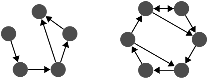
Figure 10: Two optimal graphs with a minimal Laplacian eigenvalue spread that are not generated by Algorithm 1

The paper further proves that the resulting normalized Laplacian eigenvalue spread, corresponding to the conjectured Laplacian spectrum, is indeed minimal in a couple of special cases. In this endeavor, two important lemmas, namely Lemma 21 and Lemma 22, are derived. They establish the relationships between any graph and its complement with respect to their Laplacian spectrum and eigenvalue spread. Lemma 21 implies that the complement of any graph constructed by Algorithm 1 also has the conjectured Laplacian spectrum. Moreover, Lemma 22 leads to the following important implications.

Lemma 24

A simple directed graph with $n$ vertices and $m$ arcs achieves the minimum normalized Laplacian eigenvalue spread among all such graphs if, and only if, its complement achieves the minimum normalized Laplacian eigenvalue spread among all graphs with $n$ vertices and $n(n-1)-m$ arcs.

Proof of Lemma 24: For any pair of integers $n$ and $m$ such that $n\geq 2$ and $0\leq m\leq n(n-1)$, let ${\cal G}$ denote the set of all simple directed graphs with $n$ vertices and $m$ arcs, and let $\overline{{\cal G}}$ denote the set of all simple directed graphs with $n$ vertices and $n(n-1)-m$ arcs. The complement operation defines a bijection between ${\cal G}$ and $\overline{{\cal G}}$. From Lemma 22, the graphs in ${\cal G}$ and $\overline{{\cal G}}$ share the same set of possible values for the normalized Laplacian eigenvalue spread. Therefore, their minimal possible values of normalized Laplacian eigenvalue spread are equal. It follows that a graph in ${\cal G}$ achieves the minimum normalized Laplacian eigenvalue spread among all graphs in ${\cal G}$ if and only if its complement does so among all graphs in $\overline{{\cal G}}$.  

It is worth emphasizing that Lemma 24 refers to the actual minimum normalized Laplacian eigenvalue spread, not the conjectured one. For the conjectured expression (2), we have the following result.

Lemma 25

A simple directed graph achieves the conjectured minimum normalized Laplacian eigenvalue spread given in (2) if, and only if, its complement does as well, with both equal in value.

Proof of Lemma 25: Since the complement of a graph’s complement is the graph itself, it is sufficient to prove the necessity to establish the lemma. Let $\mathbb{G}$ be any simple directed graph with $n$ vertices and $m$ arcs that achieves the conjectured minimum normalized Laplacian eigenvalue spread given in (2). We use $\sigma^{2}_{\min}(n,m)$ to denote this minimum. From Lemma 22, the complement $\overline{\mathbb{G}}$ has the same normalized Laplacian eigenvalue spread $\sigma^{2}_{\text{min}}(n,m)$. Note that $\overline{\mathbb{G}}$ has $n$ vertices and $\overline{m}=n(n-1)-m$ arcs. The conjectured minimum normalized Laplacian eigenvalue spread among all simple directed graphs with $n$ vertices and $\overline{m}$ arcs is $\sigma^{2}_{\min}(n,\overline{m})$. To show $\sigma^{2}_{\min}(n,m)=\sigma^{2}_{\min}(n,\overline{m})$, we consider two cases. First consider the case when $m$ is a multiple of $n-1$. In this case, $\kappa=\lfloor\frac{m}{n-1}\rfloor=\frac{m}{n-1}$ and $\overline{\kappa}=\lfloor\frac{\overline{m}}{n-1}\rfloor=\frac{\overline{m}}{n-1}$. From (2), $\sigma^{2}_{\min}(n,m)=\sigma^{2}_{\min}(n,\overline{m})=0$. Next consider the case when $m$ is not a multiple of $n-1$. Then, $\overline{\kappa}=n-\lceil\frac{m}{n-1}\rceil=n-\kappa-1$. With this and from (2),

$$\textstyle\sigma^{2}_{\min}(n,\overline{m}) =\textstyle\frac{1}{(n-1)^{2}}\big{[}\overline{m}-(n-1)\overline{\kappa}\big{]}\big{[}(n-1)(\overline{\kappa}+1)-\overline{m}\big{]}$$

$$=\textstyle\frac{1}{(n-1)^{2}}\big{[}(n-1)(\kappa+1)-m\big{]}\big{[}m-(n-1)\kappa\big{]}$$

$$=\sigma^{2}_{\min}(n,m).$$

Therefore, $\overline{\mathbb{G}}$ achieves the conjectured minimum normalized Laplacian eigenvalue spread, with the same value as $\mathbb{G}$.  

We can also prove the conjecture for the special cases when $m=n$ and $m=n+1$. The most important next step is to prove the conjecture in the general case. Lemmas 24 and 25 help reduce the effort by half toward this goal. It can be shown that optimal graphs are never bidirectional, except for complete graphs. To be continued.

References

- [1] A. Arenas, A. Díaz-Guilera, J. Kurths, Y. Moreno, and C. Zhou. Synchronization in complex networks. Physics Reports, 469:93–153, 2008.
- [2] T. Nishikawa and A.E. Motter. Network synchronization landscape reveals compensatory structures, quantization, and the positive effect of negative interactions. Proceedings of the National Academy of Sciences, 107(23):10342–10347, 2010.
- [3] M. Fiedler. Algebraic connectivity of graphs. Czechoslovak Mathematical Journal, 23(2):298–305, 1973.
- [4] https://en.wikipedia.org/wiki/Laplacian_matrix.
- [5] A. Cayley. A theorem on trees. Quarterly Journal of Pure and Applied Mathematics, 23:376–378, 1889.
- [6] F. Harary. Graph Theory. Addison-Wesley, 1969.
- [7] S. Geršgorin (S. Gerschgorin). Über die abgrenzung der eigenwerte einer matrix. Bulletin de l’Académie des Sciences de l’URSS. Classe des sciences mathématiques et na, 6:749–754, 1931.
- [8] R. Olfati-Saber and R.M. Murray. Consensus problems in networks of agents with switching topology and time-delays. IEEE Transactions on Automatic Control, 49(9):1520–1533, 2004.
- [9] R. Agaev and P. Chebotarev. On the spectra of nonsymmetric Laplacian matrices. Linear Algebra and its Applications, 399:157–168, 2005.
- [10] C.W. Wu. On Rayleigh-Ritz ratios of a generalized Laplacian matrix of directed graphs. Linear Algebra and its Applications, 402:207–227, 2005.
- [11] P. Chebotarev and R. Agaev. Forest matrices around the Laplacian matrix. Linear Algebra and its Applications, 356:253–274, 2002.
- [12] S. Chaiken and D.J. Klietman. Matrix tree theorems. Journal of Combinatorial Theory, Series A, 24:377–381, 1978.
- [13] D.B. West. Introduction to Graph Theory. Prentice-Hall, 2nd edition, 2000.
- [14] S. Lu, M. Gamarra, and J. Liu. Fast consensus over almost regular directed graphs. In Proceedings of the 2025 American Control Conference, 2025. to appear.