Distributionally Robust Optimization over Wasserstein Balls with i.i.d. Structure

Abstract.

Distributionally robust optimization (DRO) is a principled approach to incorporate robustness against ambiguity in the specified probabilistic models. This paper considers data-driven DRO problems with Wasserstein ambiguity sets, where the uncertain distribution splits into i.i.d. components. By exploiting the latter decomposition, we construct a tighter ambiguity set that narrows down the plausible models to product distributions only, consequently reducing the conservatism of the DRO problem. To solve the resulting nonconvex optimization problem we devise a novel sequence of convex relaxations that asymptotically converges to the true value of the original problem under mild conditions. The benefits of the approach are demonstrated via illustrative examples.

1. Introduction

In stochastic optimization a common goal is to minimize an objective $\Psi$ over a set of feasible decisions $\Theta$, where the objective $\Psi$ is defined as an average of a family of individual uncertainty-affected loss functions $\ell:\Theta\times X\to\mathbb{R}$, with $X$ being a random vector of uncertain parameters defined on a probability space $(X,\Sigma,P)$. In mathematical terms, a stochastic optimization method evaluates

(1) $$\min_{\theta\in\Theta}\Psi(\theta)\text{\ \ with\ \ }\Psi(\theta)=\mathbb{E}_{x\sim P}\ell(\theta,x)\,.$$

To avoid trivialities, we assume throughout that the feasible set $\Theta\subseteq\mathbb{R}^{m}$ and the support set $X\subseteq\mathbb{R}^{d}$ are non-empty and closed.

Problem (1) is ubiquitous in the areas of machine learning, operation research, economics, and automatic control [30]. Unfortunately, the practical deployment of (1) is complicated by the fact that the precise form of the underlying distribution $P$ is often unknown and can only be inferred indirectly from past data in the form of a finite number of samples $x_{1},\ldots,x_{n}\in X$ [7]. In this case, one can employ statistical methods to infer an estimated (parametric or non-parametric) distribution $\widehat{P}$ from the available data. However, solving (1) with the estimated $P=\widehat{P}$ may yield solutions that display poor out-of-sample performance due to the unavoidable mismatch between the true underlying distribution and $\widehat{P}$.

In distributionally robust (stochastic) optimization (DRO), the decision-maker hedges against this mismatch by minimizing the worst-case expected loss $\Psi_{\operatorname{WC}}$ with respect to all distributions in a neighborhood of $\widehat{P}$; namely the (unstructured) DRO problem is formulated as

(2) $$\min_{\theta\in\Theta}\Psi_{\operatorname{WC}}(\theta)\text{\ \ with\ \ }\Psi_{\operatorname{WC}}(\theta)=\sup_{P\in\mathcal{W}}\mathbb{E}_{x\sim P}\ell(\theta,x)\,,$$

where $\mathcal{W}\subseteq\mathcal{P}(X)$ is a set of distributions, called ambiguity set, on the space $\mathcal{P}(X)$ of all distributions supported on $X$. If appropriately chosen, the set $\mathcal{W}$ contains the true underlying distribution, which implies that any solution $\theta_{*}$ to (2) will provide an objective value of $\Psi(\theta_{*})$ lower or equal to $\Psi_{\operatorname{WC}}(\theta_{*})$ [24]. Consequently, the quality of this robust approach heavily depends on the form of the ambiguity set $\mathcal{W}$: while it should be "large enough" to include the true distribution (with high confidence), it should not contain superfluous distributions that cannot realistically appear in the problem at hand as this would lead to unnecessarily conservative solutions. Typical ambiguity sets that appear in the literature include support-, moment-, or distance-based sets of distributions or mixtures thereof [28]. While the first two types of ambiguity sets contain all distributions complying with a specified support and moment information (generally, first and second moments) [13, 26], the distance-based sets include all distributions that are within a certain given “distance” of a fixed nominal distribution. In the latter setting, the nominal distribution is often obtained through statistical techniques from available empirical data, while the distance, commonly expressed in terms of e.g. the $\phi-$divergence [2, 3], the total variation norm [31], the kernel mean embedding [19, 6], or optimal transport based-distances [29] including the celebrated Wasserstein distance [16, 24], signifies the “trust” in the statistical methods used as well as the obtained data at hand. Due to the favorable properties of Wasserstein distance in terms of expressivity and statistical properties allowing for finite-sample guarantees [15], a significant proportion of the recent literature has focused on so-called Wasserstein balls $\mathcal{W}=\mathbb{B}_{\rho}(\widehat{P})$, i.e., sets containing all distributions that are within some Wasserstein-distance $\rho>0$ from a nominal distribution $\widehat{P}$. For finitely supported nominal distributions $\widehat{P}$, the optimization of an expectation over a Wasserstein ball, which is convex, can often be reformulated into a finite-dimensional optimization program by means of Lagrange duality [16, 29], and solved efficiently via off-the-shelf solvers.

However, in several applications, the distributional uncertainty does not enter the problem at hand in an arbitrary fashion, but rather in a structured manner. One common structure consists of a set $x=(x_{1},\ldots,x_{N})$ of identically and independently distributed (i.i.d.) random variables $x_{1},\ldots,x_{N}\sim P$, where $P$ is again assumed to belong to a Wasserstein ball $\mathbb{B}_{\rho}(\widehat{P})$. This results in the structured Wasserstein distributionally robust optimization problem of the form

(3) $$\min_{\theta\in\Theta}\Psi_{\operatorname{S}}(\theta)\text{\ \ with\ \ }\Psi_{\operatorname{S}}(\theta)=\sup_{\overline{P}\in\mathcal{W}}\mathbb{E}_{x\sim\overline{P}}\ell(\theta,x)\,,$$

where $\mathcal{W}=\{P^{\otimes N}\mid P\in\mathbb{B}_{\rho}(\widehat{P})\}$ is a structured Wasserstein ambiguity set containing product distributions of the form $\overline{P}=P^{\otimes N}=P\otimes\cdots\otimes P$ only. Problem (3) arises across several domains, such as (i) control of uncertain dynamical systems, which has traditionally assumed stationarity and independence of the additive noise affecting the system dynamics; (ii) strategically robust game theory, where irrationality in the opponents’ actions is captured via a distributionally robust "best response map" that, in case of disjoint agents action sets, takes the form of (3); (iii) supply chain optimization and/or inventory management of goods with uniform popularity across buyers and shared demand drivers may be approximated as (3).

Despite the popularity of this structure in stochastic optimization, handling Problem (3) is computationally challenging. In fact, contrary to the problem of evaluating $\Psi_{\operatorname{WC}}(\theta)$, the evaluation of $\Psi_{\operatorname{S}}(\theta)$ now involves optimizing over the non-convex set $\mathcal{W}$ (the nonconvexity arises from the nonlinearity in the expectation operator due to the product structure). In turn, this prohibits the use of standard (strong) duality tools to reformulate (3) as an equivalent finite-dimensional optimization program.

1.1. Related work

While the literature concerning the (unstructured) Wasserstein DRO problem in (2) is abundant, little attention has been devoted to the case of its structured counterpart. The closest works to ours are [12, 11], where nonconvex ambiguity sets of the form

$$\mathcal{W}_{\operatorname{rect}}=\{P_{1}\otimes\cdots\otimes P_{l}\mid P_{i}\in\mathbb{B}_{\rho_{i}}(\widehat{P}_{i})\text{\ for all\ }i=1,\ldots,l\}\,.$$

are considered. For losses $\ell$ that are either additively or multiplicatively separable, a strong duality result is proven, which allows, as in the unstructured case, to compute the worst-case expectation by solving a finite-dimensional convex program. Further, [12, 11] also proposes convex overestimations of the above ambiguity set for which strong duality can be shown without requiring the restrictive separability condition.

On a different direction, [17] considers the problem of maximizing an expectation functional over a Wasserstein ambiguity set under an additional moment constraints of the form

$$\mathcal{W}_{\operatorname{mom}}=\mathbb{B}_{\rho}(\widehat{P})\cap\{P\in\mathcal{P}(\mathbb{R}^{d})\mid\mathbb{E}_{x\sim P}(x-\mu)(x-\mu)^{\top}\leq\Sigma\}\,,$$

for a-priori given mean vector $\mu\in\mathbb{R}^{d}$ and covariance matrix $\Sigma\in\mathbb{S}^{d\times d}\succeq 0$. By choosing $\Sigma$ to be diagonal, independence among the lower-dimensional components of the uncertain vector can be enforced. The resulting ambiguity set $\mathcal{W}$ retains convexity as it is described as the intersection of convex sets, allowing again to compute the worst-case expectation by means of convex programming for certain classes of loss functions, such as e.g. quadratic or piecewise affine $\ell$.

1.2. Outline and contributions

We consider data-driven DRO problems with Wasserstein ambiguity sets, where the uncertainty affects the problem in an i.i.d. fashion, as in (3). Consider the inner supremum problem

(4) $$\sup_{\overline{P}\in\mathcal{W}}\mathbb{E}_{x\sim\overline{P}}\ell(x)\text{\ \ with\ \ }\mathcal{W}=\{P^{\otimes N}\mid P\in\mathbb{B}_{\rho}(\widehat{P})\}\,.$$

After introducing the necessary background in Section 2, we establish conditions under which (4) is finite and attains its optimum in Section 3.1. Moreover, there we also show that (4) can be upper-bounded by a standard Wasserstein DRO problem. Next, in Section 3.2 we show that the latter upper bound is in general conservative and propose a potentially tighter upper bound based on symmetrization of the corresponding loss $\ell$ that allows for strong duality. Further, in Section 3.3, using the concept of lifting and based on the previous bound, we introduce a nonincreasing sequence of upper bounds (relaxations) on (4) that admit strong duality. We investigate the properties of this sequence of relaxations in Section 3.4. As a main result, in Section 3.5, we show in Theorem 8 that the gap between the lower bound of the relaxation sequence and (4) vanishes if $\ell$ is concave. Additionally, in Section 3.6 we show that for sets of the form $\mathcal{W}$ our upper bound established in Section 3.2 is less conservative than an upper bound provided in [11]. Finally, in Section 4.1 we formulate the strong duality for the relaxation sequence as a second order cone program whenever $\ell$ is a polyhedral loss function and provide some numerical examples.

2. Notation and Preliminaries

In this section we recapitulate some well-known results about the Wasserstein distance and Wasserstein distributionally robust optimization. For a more throughout introduction we refer to [33, 23]. For any measurable space $(X,\mathcal{X})$ we denote by $\mathcal{P}(X)$ the set of probability measures on $(X,\mathcal{X})$. Given two measure spaces $(X,\mathcal{X})$, $(Y,\mathcal{Y})$, a measurable map $f:X\to Y$ and $P\in\mathcal{P}(X)$, then $f\#P\in\mathcal{P}(Y)$ denotes the pushforward distribution defined by $f\#P(A)=P(f^{-1}(A))$ for all $A\in\mathcal{Y}$. We denote the product space $X^{N}=X\times\cdots\times X$ for $N\in\mathbb{N}$ and the projections $\operatorname{pr}_{i}:X^{N}\to X$ onto the $i$-th coordinate. If $M\geq N$ is an integer, then by $\operatorname{pr}_{1:N}^{M}:X^{M}\to X^{N}$ we denote the projection onto the first $N$ factors of $X^{M}$. Finally, if $M$ is clear from the context, then it is omitted: $\operatorname{pr}_{1:N}=\operatorname{pr}_{1:N}^{M}$. If $X$ is a Polish space, then we set $\mathcal{X}=\mathcal{B}(X)$ to be the Borel $\sigma$-algebra and omit $\mathcal{X}$ from the notation altogether. For two distributions $P_{1},P_{2}\in\mathcal{P}(X)$ we denote by $\Gamma(P_{1},P_{2})$ the set of all couplings of $P_{1}$ and $P_{2}$, i.e. all $\Lambda\in\mathcal{P}(X\times X)$ such that $\operatorname{pr}_{i}\#\Lambda=P_{i}$ for $i=1,2$. A (transportation) cost $c:X\times X\to[0,\infty)$ is a lower semi-continuous and symmetric function such that $c(x,x)=0$ for all $x\in X$. Then the Wasserstein distance between two probability measures $P_{1},P_{2}\in\mathcal{P}(X)$ is defined as

(5) $$W_{c}(P_{1},P_{2})=\inf_{\Lambda\in\Gamma(P_{1},P_{2})}\int c(x,y)\,\text{d}\Lambda(x,y)\,.$$

Intuitively the value $W_{c}(P_{1},P_{2})$ measures the total cost of moving a “pile” of mass distributed according to $P_{1}$ to a pile distributed according to $P_{2}$ if the cost of moving a unit of mass located in $x\in X$ to $y\in X$ is $c(x,y)$ [21, 9, 32, 33]. If finite, the infimum in (5) is attained [33, Theorem 4.1] and $\Gamma_{c}(P_{1},P_{2})$ will denote the set of minimizers. We say that the cost $c$ satisfies the weak triangle inequality (other terminology: quasi-triangle-inequality or $K$-relaxed triangle inequality) if there exists a constant $K>0$ such that $c(x,y)\leq K(c(x,z)+c(z,y))$ for all $x,y,z\in X$. In this case the set $\mathcal{P}_{c}(X)=\{P\in\mathcal{P}(X)\mid\int c(x_{0},\cdot)\,\text{d}P<\infty\}$ is independent of $x_{0}\in X$ and convex. The cost $c$ is called proper if it satisfies the weak triangle inequality and the sublevel sets $\{x\in X\mid c(x_{0},x)\leq r\}$ are compact for all $r>0$ and $x_{0}\in X$. If $d$ is a metric on $X$, then $W_{p}$ defined by $W_{p}(P_{1},P_{2})=W_{c}(P_{1},P_{2})^{1/p}$ with $c(x,y)=d(x,y)^{p}$ is a metric on the set $\mathcal{P}_{p}(X):=\mathcal{P}_{c}(X)$ of all distributions with finite $p$-th moment [33, 25]. Further for $\widehat{P}\in\mathcal{P}_{c}(X)$ and $\rho>0$ we will denote $\mathbb{B}_{\rho}^{c}(\widehat{P})=\{P\in\mathcal{P}_{c}(X)\mid W_{c}(P,\widehat{P})\leq\rho\}$ for the $W_{c}$-Wasserstein ball of radius $\rho$ around $\widehat{P}$. The Lebesgue spaces on the measure space $(X,P)=(X,\mathcal{B}(X),P)$ are denoted by $L^{p}(X,P)$. Finally, the symbol $\mathcal{S}_{N}$ denotes symmetric group on $N$ letters, while $\mathcal{S}_{\infty}$ denotes the set of all bijections $\pi:\mathbb{N}\to\mathbb{N}$ that leave all but finitely many indices invariant. Moreover, we always identify a $\pi\in\mathcal{S}_{N}$ with the induced coordinate permutation $\pi:X^{N}\to X^{N}:x\mapsto(x_{\pi}(k))_{k=1}^{N}$.

Consider now the Wasserstein distributionally robust optimization [23, 29] of the type

(6) $$\sup_{P\in\mathbb{B}_{\rho}^{c}(\widehat{P})}\mathbb{E}_{x\sim P}\ell(x)$$

where $\ell:X\to\mathbb{R}$ is a Borel measurable loss functional and (6) corresponds to the inner problem of (2) with $\ell=\ell(\theta,\cdot)$ for a fixed $\theta$. To study the finiteness and existence of optimizers, define $\mathcal{D}=\{\delta:[0,\infty)\to[0,\infty)\mid\forall r>0:\,\delta(r)\leq r\,,\;\lim_{r\to\infty}\frac{\delta(r)}{r}=0\}$ and consider the following function growth classes:

$$\mathcal{G}_{c}(X) =\{\ell:X\to\mathbb{R}\mid\exists C>0\,,x_{0}\in X\,:\;\ell\leq C(1+c(x_{0},\cdot))\}\,,$$

$$\mathcal{G}_{c}^{<}(X) =\{\ell:X\to\mathbb{R}\mid\exists\delta\in\mathcal{D}\,,x_{0}\in X\,:\;\ell\leq C(1+\delta(c(x_{0},\cdot)))\}\,.$$

The following result establishes the well-posedness of the problem formulation in (6).

Theorem 1.

For any Borel $\ell:X\to\mathbb{R}$ the value of (6) is finite if $c$ satisfies the weak triangle inequality, $\widehat{P}\in\mathcal{P}_{c}(X)$ and $\ell\in\mathcal{G}_{c}(X)$. Moreover, if $c$ is proper, $\ell$ is upper semi-continuous and $\ell\in\mathcal{G}_{c}^{<}(X)$, then the optimal value of (6) is attained.

For the case of $c=d^{p}$ the result has been established in [35], where the authors considered $\delta(r)=\min\{r^{\widetilde{p}/p},r\}$ for some $\widetilde{p}\in[1,p)$. Now, even though the optimization problem (6) is infinite-dimensional, it is convex, since the objective is linear and the constraint set $\mathbb{B}_{\rho}^{c}(\widehat{P})$ convex in the ambiguous distribution $P$. The following theorem provides a strong duality result [16, 8, 29, 36].

Theorem 2 ([16]).

Let $\ell\in L^{1}(X,\widehat{P})$ and $\rho>0$. Then the value of (6) is equal to

$$\sup_{\overline{P}\in\mathcal{W}}\mathbb{E}_{x\sim\overline{P}}\ell(x)=\inf_{\mu\geq 0}\mu\rho+\mathbb{E}_{z\sim\widehat{P}}\phi_{\mu}(z)$$

where the infimum is attained and $\phi_{\mu}:X\to\overline{\mathbb{R}}:z\mapsto\sup_{x\in X}(\ell(x)-\mu c(x,z))$ is universally measurable [5, 4].

The main importance of this theorem is that it reduces the infinite-dimensional problem (6) to a finite-dimensional problem over a single scalar variable $\mu\geq 0$, provided that the expectation of $\phi_{\mu}$ w.r.t. $\widehat{P}$ can be computed explicitly.

3. Structured Distributionally Robust Optimization

In this section, we are interested in the inner optimization problems of (3), namely

(7) $$\sup_{\overline{P}\in\mathcal{W}}\mathbb{E}_{x\sim\overline{P}}\ell(x)=\sup_{P\in\mathbb{B}_{\rho}^{c}(\widehat{P})}\int\ell(x)\,\text{d}P^{\otimes N}(x)\,,$$

for some $N\in\mathbb{N}$, Borel measurable $\ell:X^{N}\to\mathbb{R}$ and

(8) $$\mathcal{W}=\{P^{\otimes N}\mid P\in\mathbb{B}_{\rho}^{c}(\widehat{P})\}\,.$$

In its stated form problem (7) is non-convex, since the set $\mathcal{W}$ is non-convex. The proofs of the subsequent results are confined to the appendix.

3.1. Finiteness and existence of optimizers

First we will delve into when (7) is well-defined, finite and attains its solution on $\mathcal{W}$. For $N\in\mathbb{N}$ we write $c^{N}:X^{N}\times X^{N}\to[0,\infty):(x,y)\mapsto\sum_{i=1}^{N}c(x_{i},y_{i})$ for the $N$-lift of the transport cost $c$. In some cases we will omit the superscript $N$ and write again $c$ instead of $c^{N}$ for brevity. Note that the $N$-lift of $c=d^{p}$ is of the same form as well, namely $c^{N}=(d_{N})^{p}$, where $d_{N}(x,y)=(\sum_{i=1}^{N}d(x_{i},y_{i})^{p})^{1/p}$. Here $d_{N}$ is a metric which induces the product topology on $X^{N}$.

To start, we note that for $N\in\mathbb{N}$ the set $\mathcal{W}$ can be overestimated by an ordinary Wasserstein ball w.r.t. a modified transportation cost.

Lemma 1.

For any transportation cost $c:X\times X\to[0,\infty]$, $P_{1},P_{2}\in\mathcal{P}(X)$, $\rho\geq 0$ and $N\in\mathbb{N}$ it holds that $P^{\otimes N}\in\mathbb{B}_{N\rho}^{c^{N}}(\widehat{P}^{\otimes N})$ for all $P\in\mathbb{B}_{\rho}^{c}(\widehat{P})$.

Thus

(9) $$\mathcal{W}\subseteq\mathbb{B}_{N\rho}^{c^{N}}(\widehat{P}^{\otimes N})\,.$$

and it always holds that

(10) $$\sup_{\overline{P}\in\mathcal{W}}\mathbb{E}_{x\sim\overline{P}}\ell(x)\leq\sup_{\overline{P}\in\mathbb{B}_{N\rho}^{c^{N}}(\widehat{P}^{\otimes N})}\mathbb{E}_{x\sim\overline{P}}\ell(x)\,,$$

and we can use a Theorem 1 to conclude that the value of (7) is finite if $\ell\in\mathcal{G}_{c^{N}}(X^{N})$, or equivalently,

(11) $$\ell(x) \leq C\left(1+\sum_{k=1}^{N}c(x_{0},x_{k})\right)\text{\ \ for all\ \ }x\in X^{N}\text{\ for some\ }C>0\,,\;x_{0}\in X\,.$$

However, because of the product structure of $\mathcal{W}$ it is actually enough to require argument-wise growth conditions. For this purpose define the following function growth classes

$$\widehat{\mathcal{G}}_{c,N}(X^{N})$$

$$\quad=\left\{\ell:X^{N}\to\mathbb{R}\mid\exists C>0\,,x_{0}\in X\,,\forall x\in X^{N}:\;\ell(x)\leq C\prod_{k=1}^{N}(1+c(x_{0},x_{k}))\right\}\,,$$

$$\widehat{\mathcal{G}}_{c,N}^{<}(X^{N})$$

$$\quad=\left\{\ell:X^{N}\to\mathbb{R}\mid\exists\delta\in\mathcal{D}\,,x_{0}\in X\,,\forall x\in X^{N}:\;\ell(x)\leq C\prod_{k=1}^{N}(1+\delta(c(x_{0},x_{k})))\right\}\,.$$

Note that in general $\mathcal{G}_{c^{N}}(X^{N})\subsetneq\widehat{\mathcal{G}}_{c,N}(X^{N})$ and $\mathcal{G}_{c^{N}}^{<}(X^{N})\subsetneq\widehat{\mathcal{G}}_{c,N}^{<}(X^{N})$. Then we have the following analogon of Theorem 1.

Theorem 3.

For any Borel $\ell:X^{N}\to\mathbb{R}$ the value of (6) is finite if $c$ satisfies the weak triangle inequality, $\widehat{P}\in\mathcal{P}_{c}(X)$ and $\ell\in\widehat{\mathcal{G}}_{c,N}(X^{N})$. Moreover, if $c$ is proper, $\ell$ is upper semi-continuous and $\ell\in\widehat{\mathcal{G}}_{c,N}^{<}(X^{N})$, then the optimal value of (6) is attained.

3.2. A convex upper bound

In the previous section we have seen that (10) states an upper bound on (7). In general this bound will be conservative as the following example shows.

Example 1.

Let $X=\mathbb{R}$, $N=2$, $c(x_{1},x_{2})=\lvert x_{1}-x_{2}\rvert^{2}$, $\widehat{P}=\delta_{0}$ and $\ell(x_{1},x_{2})=\frac{1}{2}(x_{1}-x_{2})^{2}$. Then the value of the structured problem is

$$\sup_{P\in\mathbb{B}_{\rho}^{c}(\widehat{P})}\mathbb{E}_{x\sim P^{\otimes 2}}\ell(x)=\sup_{P\in\mathbb{B}_{\rho}^{c}(\delta_{0})}\operatorname{Var}(P)=\sup_{\mathbb{E}(\widehat{P}^{2})\leq\rho}\mathbb{E}(P^{2})-(\mathbb{E}P)^{2}\leq\rho\,,$$

with $P=\frac{1}{2}\delta_{-\sqrt{\rho}}+\frac{1}{2}\delta_{\sqrt{\rho}}$ showing that in fact the latter bound is attained. On the other hand, the value of the right hand side of (10) can be computed using Theorem 2 and is given by

$$\sup_{\overline{P}\in\mathbb{B}_{2\rho}^{c}(\delta_{0}^{\otimes 2})}\mathbb{E}_{x\sim\overline{P}}\ell(x)=\inf_{\mu\geq 0}\left[2\rho\mu+\sup_{x\in\mathbb{R}^{2}}\left(\frac{1}{2}(x_{1}-x_{2})^{2}-\mu\lVert x\rVert^{2}\right)\right]=2\rho\,.$$

The next example shows that the conservatism of this bound can be arbitrary large in a relative sense.

Example 2.

Let $X=\mathbb{R}$, $N=2$, $c(x_{1},x_{2})=\lvert x_{1}-x_{2}\rvert^{2}$, $\widehat{P}=\frac{1}{2}\delta_{1}+\frac{1}{2}\delta_{-1}$ and $\ell(x_{1},x_{2})=-x_{1}x_{2}$. Then the value of the structured problem is

$$\sup_{P\in\mathbb{B}_{\rho}^{c}(\widehat{P})}\mathbb{E}_{x\sim P^{\otimes 2}}\ell(x)=\sup_{P\in\mathbb{B}_{\rho}^{c}(\widehat{P})}-(\mathbb{E}P)^{2}=0\,.$$

The value of the right hand side of (10) is, after some elementary calculations, given by

$$\sup_{\overline{P}\in\mathbb{B}_{2\rho}^{c}(\widehat{P}^{\otimes 2})}\mathbb{E}_{x\sim\overline{P}}\ell(x) =\inf_{\mu\geq 0}\left[2\rho\mu+\frac{1}{4}\sum_{\widehat{\xi}\in\{\pm 1\}^{2}}\sup_{x\in\mathbb{R}^{2}}\left(-x_{1}x_{2}-\mu\lVert x-\widehat{\xi}\rVert^{2}\right)\right]$$

$$=\inf_{\mu>\frac{1}{2}}\left[2\rho\mu-\frac{2\mu}{1-4\mu^{2}}\right]$$

$$\geq\rho\,.$$

Hence, while the value of the structured problem is constant, the value of the latter bound grows asymptotically linearly as the ball radius increases.

In view of the last two examples we turn to the question whether we can obtain better bounds on (7) than (10). This corresponds to obtaining tighter convex overestimations of the set $\mathcal{W}$ than the one given by (9). Clearly, the best such overestimation is the convex hull $\operatorname{conv}\mathcal{W}$ and indeed even more is true.

Lemma 2.

If $\ell\in L^{1}(X^{N},P^{\otimes N})$ for all $P\in\mathbb{B}_{\rho}^{c}(\widehat{P})$, then

$$\sup_{\overline{P}\in\mathcal{W}}\mathbb{E}_{x\sim\overline{P}}\ell(x)=\sup_{\overline{P}\in\operatorname{conv}\mathcal{W}}\mathbb{E}_{x\sim\overline{P}}\ell(x)=\sup_{\overline{P}\in\overline{\operatorname{conv}}^{\operatorname{w}}\mathcal{W}}\mathbb{E}_{x\sim\overline{P}}\ell(x)\,,$$

where $\overline{\operatorname{conv}}^{\operatorname{w}}\mathcal{W}$ is the closure of $\operatorname{conv}\mathcal{W}$ in the weak topology of $\mathcal{P}(X)$.

The nontrivial part is the second equality, since the first equality is simply a consequence of the expectation being linear in the distribution. Note that by Theorem 3 the condition $\ell\in L^{1}(X^{N},P^{\otimes N})$ for all $P\in\mathbb{B}_{\rho}^{c}(\widehat{P})$ holds if e.g. $\ell\in\widehat{\mathcal{G}}_{c,N}(X^{N})$.

While this shows that our original non-convex DRO problem can be reformulated as a convex problem, it is very difficult to exhibit an explicit description of the sets $\operatorname{conv}\mathcal{W}$ or $\overline{\operatorname{conv}}^{\operatorname{w}}\mathcal{W}$ that would make the latter computationally tractable. Hence we proceed to search for convex sets that overestimate $\overline{\operatorname{conv}}^{\operatorname{w}}\mathcal{W}$, while still being a subset of $\mathbb{B}_{N\rho}^{c^{N}}(\widehat{P}^{\otimes N})$ and allowing for strong duality in the sense of Theorem 2. For this we explore (7) further and define

(12) $$\operatorname{S}(\ell)=\sup_{\overline{P}\in\mathcal{W}}\mathbb{E}_{x\sim\overline{P}}\ell(x)\,,\quad\operatorname{U}(\ell)=\sup_{\overline{P}\in\mathbb{B}_{N\rho}^{c^{N}}(P^{\otimes N})}\mathbb{E}_{x\sim\overline{P}}\ell(x)\,.$$

Then, (10) translates simply to $\operatorname{S}(\ell)\leq\operatorname{U}(\ell)$ for any Borel $\ell:X^{N}\to\mathbb{R}$. Note that $\operatorname{U}(\ell)$ is a DRO problem of the type (6) and hence can be computed by using Theorem 2. Now suppose that we can find some set $\mathcal{F}$ of transformations $F:\mathbb{R}^{X^{N}}\to\mathbb{R}^{X^{N}}$ such that $\operatorname{id}\in\mathcal{F}$, $F(\ell)$ is Borel measurable for any Borel measurable $\ell:X^{N}\to\mathbb{R}$ and

(13) $$\operatorname{S}(F(\ell))=\operatorname{S}(\ell)\text{\ \ for all\ \ }F\in\mathcal{F}\text{\ and Borel\ }\ell:X^{N}\to\mathbb{R}\,.$$

Then we obtain for any Borel $\ell:X^{N}\to\mathbb{R}$ that

$$\operatorname{S}(\ell)=\operatorname{S}(F(\ell))\leq\operatorname{U}(F(\ell))$$

and hence

(14) $$\operatorname{S}(\ell)\leq\inf_{F\in\mathcal{F}}\operatorname{U}(F(\ell))$$

is a potentially better upper bound on $\operatorname{S}(\ell)$ than $\operatorname{U}(\ell)$. To obtain such a class $\mathcal{F}$ we make the following, crucial observation: If $\pi\in\mathcal{S}_{N}$ is a permutation, then the transformation $F_{\pi}:\ell\mapsto\ell_{\pi}$ with $\ell_{\pi}(x)=\ell(\pi(x))$, where $\pi(x)=(x_{\pi(1)},\ldots,x_{\pi(N)})$ for $x\in X^{N}$, satisfies

$$\operatorname{S}(F_{\pi}(\ell))=\sup_{\overline{P}\in\mathcal{W}}\mathbb{E}_{x\sim\overline{P}}\ell_{\pi}(x)=\sup_{P\in\mathbb{B}_{\rho}^{c}(\widehat{P})}\mathbb{E}_{x\sim P^{\otimes N}}\ell_{\pi}(x)=\sup_{P\in\mathbb{B}_{\rho}^{c}(\widehat{P})}\mathbb{E}_{x\sim P^{\otimes N}}\ell(x)=\operatorname{S}(\ell)\,,$$

since $\pi\#P^{\otimes N}=P^{\otimes N}$ for any permutation $\pi$. Moreover, since $\mathbb{E}_{x\sim\overline{P}}\ell$ is linear in $\ell$, it follows that (13) holds for

(15) $$\mathcal{F}=\operatorname{conv}\{F_{\pi}\mid\pi\in\mathcal{S}_{N}\}=\left\{F_{\alpha}=\sum_{\pi\in\mathcal{S}_{N}}\alpha_{\pi}F_{\pi}\mid\alpha\in\Delta^{\mathcal{S}_{N}}\right\}\,,$$

where $\Delta^{\mathcal{S}_{N}}=\{\alpha=(\alpha_{\pi})_{\pi\in\mathcal{S}_{N}}\in[0,1]^{\mathcal{S}_{N}}\mid\sum_{\pi\in\mathcal{S}_{N}}\alpha_{\pi}=1\}$ is the standard simplex in the $N!$-dimensional Euclidean space. This implies that (14) holds for the above class $\mathcal{F}$ of transformations. In this specific case we can actually establish the following

Lemma 3.

For any Borel measurable $\ell:X^{N}\to\mathbb{R}$ it holds that

$$\inf_{F\in\mathcal{F}}\operatorname{U}(F(\ell))=\min_{\alpha\in\Delta^{\mathcal{S}_{N}}}\operatorname{U}(F_{\alpha}(\ell))=\operatorname{U}(\ell_{\operatorname{sym}})\,,$$

where the symmetrization of a function is defined by

(16) $$\ell_{\operatorname{sym}}(x)=\frac{1}{N!}\sum_{\pi\in\mathcal{S}_{N}}\ell(\pi(x))\,,$$

i.e. the infimum in (14) is attained in the uniform coefficient $\alpha=(1/N!,\ldots,1/N!)\in\Delta^{\mathcal{S}_{N}}$.

Thus instead of optimizing over the class $\mathcal{F}$ as in (14), we can replace the latter by the single upper bound

(17) $$\operatorname{S}(\ell)\leq\operatorname{U}(\ell_{\operatorname{sym}})\,.$$

Example 3.

Let $X=\mathbb{R}$, $N=2$, $c(x_{1},x_{2})=\lvert x_{1}-x_{2}\rvert^{2}$, $\widehat{P}=\frac{1}{2}\delta_{1}+\frac{1}{2}\delta_{-1}$ and $\ell(x_{1},x_{2})=-2x_{1}^{2}-2x_{1}x_{2}$. Then the value of the structured problem is given by

$$\operatorname{S}(\ell)=\operatorname{S}(\ell_{\operatorname{sym}})=\sup_{P\in\mathbb{B}_{\rho}^{c}(\widehat{P})}-2(\mathbb{E}(P^{2})+(\mathbb{E}P)^{2})=-2(1-\min(\sqrt{\rho},1))^{2}\leq 0\,.$$

The value of the unstructured bound is, after some elementary calculations,

$$\operatorname{U}(\ell)=\inf_{\mu>\sqrt{2}-1}2\rho\mu+\frac{2\mu(1-\mu)}{\mu(\mu+2)-1}\geq(\sqrt{2}-1)2\rho-2\,,$$

while the value of the symmetrized bound is

$$\operatorname{U}(\ell_{\operatorname{sym}})=2(2\sqrt{2\min(\rho,1/2)}-2\min(\rho,1/2)-1)\leq 0\,.$$

See Figure 1(a) for a graphical illustration.

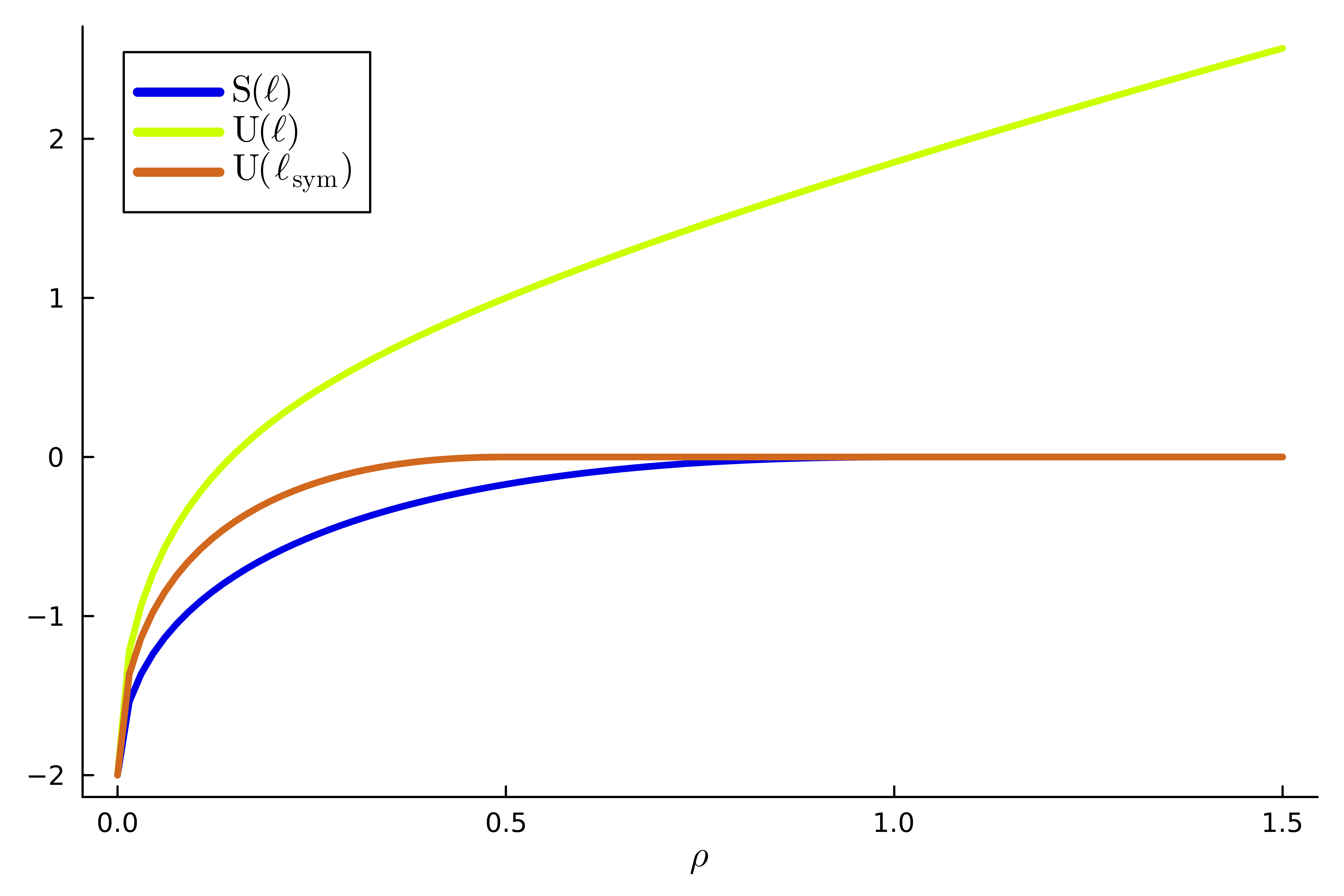
(a) Objective values for Example 3

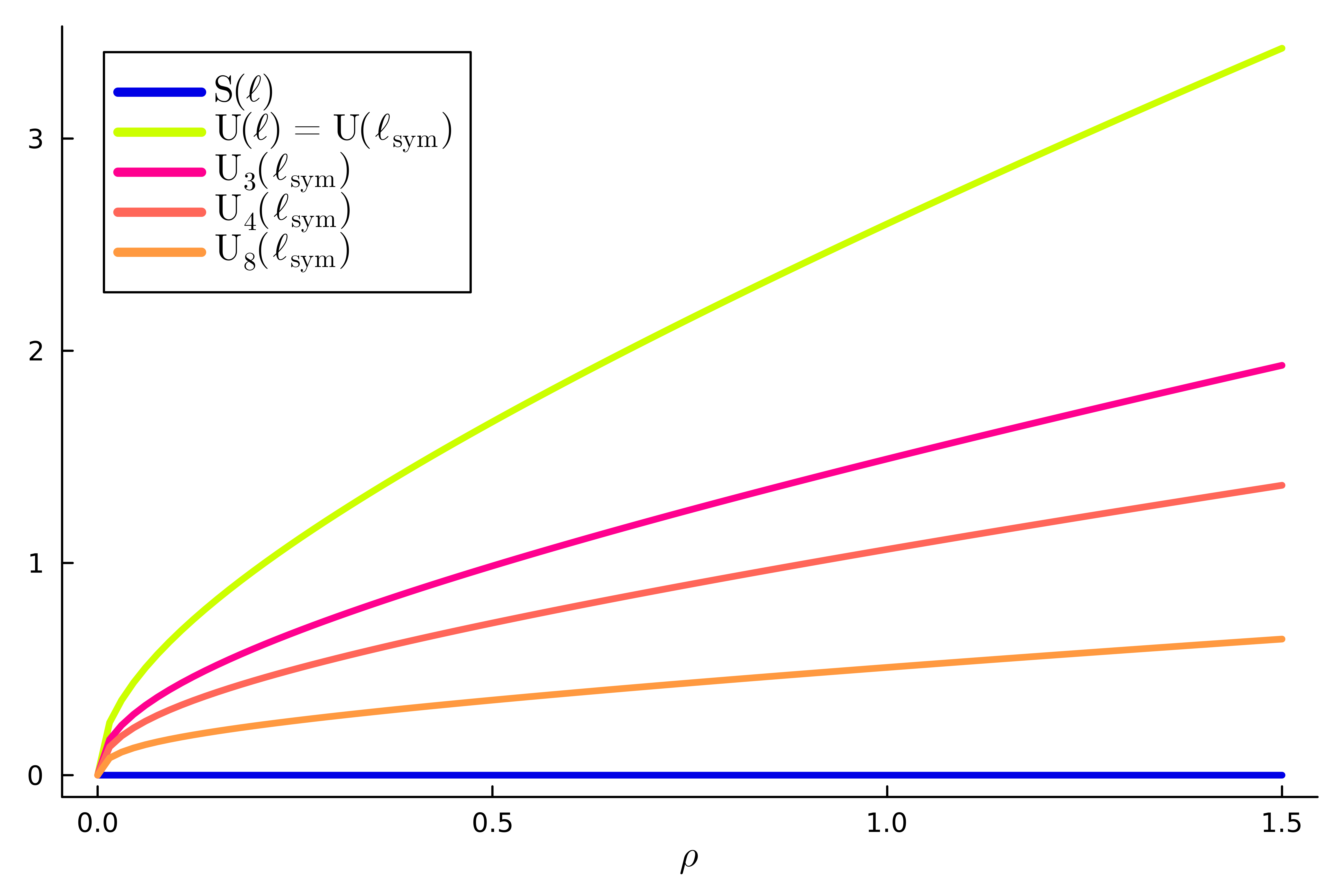
(b) Objective values for Example 4

Figure 1. Objective values for Examples 3 and 4

For the purpose of interpreting the upper bound $\operatorname{U}(\ell_{\operatorname{sym}})$ in terms of an overestimation of the set $\overline{\operatorname{conv}}^{\operatorname{w}}\mathcal{W}$ we need the following

Definition 1.

A distribution $\overline{P}\in\mathcal{P}(X^{N})$ is called symmetric (other terminology: exchangeable or permutation-invariant) if for any permutation $\pi\in\mathcal{S}_{N}$ it holds that $\pi\#\overline{P}=\overline{P}$. The set of symmetric distributions on $X^{N}$ is denoted by $\mathcal{P}_{\operatorname{sym}}(X^{N})$.

One important example are powers of distributions $\overline{P}=P^{\otimes N}$, which are always symmetric. Additionally and in analogy to (16) let us write

(18) $$\overline{P}_{\operatorname{sym}}:=\frac{1}{N!}\sum_{\pi\in\mathcal{S}_{N}}\pi\#\overline{P}$$

for the symmetrization of the distribution $\overline{P}$. This yields the following

Theorem 4.

Suppose that $\ell\in\mathcal{G}_{c^{N}}(X^{N})$ is Borel measurable. Then

(19) $$\begin{aligned} \operatorname{U}(\ell_{\operatorname{sym}})=\sup_{\overline{P}\in\mathbb{B}_{N\rho}^{c^{N}}(\widehat{P}^{\otimes N})_{\operatorname{sym}}}\int\ell\,\text{d}\overline{P}\,,\end{aligned}$$

where

(20) $$\mathbb{B}_{N\rho}^{c^{N}}(\widehat{P}^{\otimes N})_{\operatorname{sym}}:=\{\overline{P}_{\operatorname{sym}}\mid\overline{P}\in\mathbb{B}_{N\rho}^{c^{N}}(\widehat{P}^{\otimes N})\}=\mathbb{B}_{N\rho}^{c^{N}}(\widehat{P}^{\otimes N})\cap\mathcal{P}_{\operatorname{sym}}(X^{N})\,,$$

From (19) we make two observations: Firstly, the upper bound $\operatorname{U}(\ell_{\operatorname{sym}})$ corresponds to optimizing over the set (20) contains $\overline{\operatorname{conv}}^{\operatorname{w}}\mathcal{W}$, since it is weakly closed, convex and contains $\mathcal{W}$. Secondly we see that even though the set $\mathbb{B}_{N\rho}^{c^{N}}(P^{\otimes N})_{\operatorname{sym}}$ is not a Wasserstein ball itself, one can still evaluate the corresponding DRO problem

(21) $$\sup_{\overline{P}\in\mathbb{B}_{N\rho}^{c^{N}}(P^{\otimes N})_{\operatorname{sym}}}\int\ell\,\text{d}\overline{P}$$

using Theorem 2 by evaluating $\operatorname{U}(\ell_{\operatorname{sym}})$, i.e. by substituting $\ell$ with $\ell_{\operatorname{sym}}$ and replacing $\mathbb{B}_{N\rho}^{c^{N}}(P^{\otimes N})_{\operatorname{sym}}$ by $\mathbb{B}_{N\rho}^{c^{N}}(P^{\otimes N})$ in (6).

3.3. Sequence of convex relaxations

It is interesting to ask now whether we can find even tighter overestimations of $\overline{\operatorname{conv}}^{\operatorname{w}}\mathcal{W}$ than $\mathbb{B}_{N\rho}^{c^{N}}(P^{\otimes N})_{\operatorname{sym}}$. In view of (20) the latter question is equivalent determining what distinguishes powers of measures in the set of all symmetric measures. The crucial observation is that powers of powers of measures are again powers of measures and hence symmetric, while the same does not have to be true for general symmetric measures. This latter viewpoint hints us to lift our problem and consider instead of (7) the problem

(22) $$\sup_{P\in\mathbb{B}_{\rho}^{c}(\widehat{P})}\int\ell\circ\operatorname{pr}_{1:N}^{M}(x)\,\text{d}P^{\otimes M}(x)\,,$$

where $N\leq M\leq\infty$ is a “lifting parameter” and $\operatorname{pr}_{1:N}^{M}:X^{M}\to X^{N}$ is the projection onto the first $N$ components, i.e. in (22) we see the function $\ell$ on $X^{N}$ as a function $\widehat{\ell}=\ell\circ\operatorname{pr}_{1:N}^{M}$ on $X^{M}$. Analogously we define the quantities

$$\operatorname{S}_{M}(\widehat{\ell}):=\sup_{P\in\mathbb{B}_{\rho}^{c}(\widehat{P})}\mathbb{E}_{x\sim P^{\otimes M}}\widehat{\ell}(x)\leq\operatorname{U}_{M}(\widehat{\ell}):=\sup_{\overline{P}\in\mathbb{B}_{M\rho}^{c^{M}}(P^{\otimes M})}\mathbb{E}_{x\sim\overline{P}}\widehat{\ell}(x)\,.$$

Note that (22) has the same optimal value as (7), since integrating w.r.t. extra factors $P$ does not change the value of the integral, i.e. $\operatorname{S}_{N}(\ell)=\operatorname{S}_{M}(\ell\circ\operatorname{pr}_{1:N}^{M})$ for any $M\geq N$. In view of (17) it then follows that

$$\operatorname{S}(\ell)=\operatorname{S}_{N}(\ell)=\operatorname{S}_{M}(\widehat{\ell})\leq\operatorname{U}_{M}(\widehat{\ell}_{\operatorname{sym}})\text{\ \ for\ \ }N\leq M<\infty\,.$$

Note that here $\widehat{\ell}_{\operatorname{sym}}$ denotes the symmetrization of $\ell$ viewed as a function $X^{M}\to\mathbb{R}$ and thus itself depends on $M$. To summarize, for each $M\geq N$ we obtain an upper bound

(23) $$\operatorname{U}_{M}^{\operatorname{sym}}(\ell):=\operatorname{U}_{M}((\ell\circ\operatorname{pr}_{1:N}^{M})_{\operatorname{sym}})$$

on $\operatorname{S}(\ell)$. It then holds that

(24) $$\operatorname{S}(\ell)\leq\operatorname{U}_{\infty}^{\operatorname{sym}}(\ell):=\inf_{M\geq N}\operatorname{U}_{M}^{\operatorname{sym}}(\ell)\,.$$

We stress again that, contrary to the original problem $\operatorname{S}(\ell)$, we can evaluate each $\operatorname{U}_{M}^{\operatorname{sym}}(\ell)$ via Theorem 2 by using the relation (23). For notational brevity we also set $\operatorname{U}_{0}^{\operatorname{sym}}(\ell):=\operatorname{U}(\ell)$ for the non-symmetrized bound defined as the right side of (10).

Example 4.

Let $X$, $N$, $c$, $\widehat{P}$ and $\ell$ be as in Example 2. After some elementary calculations we obtain

$$\operatorname{U}_{M}^{\operatorname{sym}}(\ell) =\inf_{\mu>\frac{1}{M(M-1)}}M(\rho-1)\mu+\frac{(M-1)M^{2}\mu^{2}}{(M-1)M\mu-1}\left(1-\frac{1}{(M-1)(1+M\mu)}\right)$$

$$\leq\inf_{\mu>\frac{1}{M(M-1)}}M(\rho-1)\mu+\frac{(M-1)M^{2}\mu^{2}}{(M-1)M\mu-1}$$

$$=\frac{(\sqrt{\rho}+1)^{2}}{M-1}\,,$$

i.e. for a fixed $\rho>0$ it follows $\lim_{M\to\infty}\operatorname{U}_{M}^{\operatorname{sym}}(\ell)=0=\operatorname{S}(\ell)$. See Figure 1(b) for a graphical illustration.

In view of Example 4 it is now natural to ask under which conditions the inequality in (23) is an equality, i.e. when the sequence of relaxations is tight and there is no relaxation gap. For this we will investigate this gap in the next section in more detail.

3.4. Relaxation gap

To understand the gap between $\operatorname{S}(\ell)$ and $\operatorname{U}_{\infty}^{\operatorname{sym}}(\ell)$ it is helpful to first understand the lifting relaxation $\operatorname{U}_{M}^{\operatorname{sym}}(\ell)$ in terms of overestimations of $\overline{\operatorname{conv}}^{\operatorname{w}}\mathcal{W}$. For this purpose we unfold the definitions to obtain

$$\begin{gathered}\operatorname{U}_{M}^{\operatorname{sym}}(\ell)=\sup_{\overline{P}\in\mathbb{B}_{M\rho}^{c^{M}}(\widehat{P}^{\otimes M})}\int(\ell\circ\operatorname{pr}_{1:N}^{M})_{\operatorname{sym}}\,\text{d}\overline{P}=\sup_{\overline{P}\in\mathbb{B}_{M\rho}^{c^{M}}(\widehat{P}^{\otimes M})}\int\ell\circ\operatorname{pr}_{1:N}^{M}\,\text{d}\overline{P}_{\operatorname{sym}}\\ =\sup_{\overline{P}\in\mathbb{B}_{M\rho}^{c^{M}}(\widehat{P}^{\otimes M})}\int\ell\,\text{d}(\operatorname{pr}_{1:N}^{M}\#\overline{P}_{\operatorname{sym}})=\sup_{\overline{P}\in\mathcal{U}_{M}}\int\ell\,\text{d}\overline{P}\,,\end{gathered}$$

with

(25) $$\mathcal{U}_{M}:=\{\operatorname{pr}_{1:N}^{M}\#\overline{P}\mid\overline{P}\in\mathbb{B}_{M\rho}^{c^{M}}(\widehat{P}^{\otimes M})_{\operatorname{sym}}\}\subseteq\mathcal{P}(X^{N})\,,$$

i.e. we overestimate $\overline{\operatorname{conv}}^{\operatorname{w}}\mathcal{W}$ by sets of the form (25), which consist of all marginal distributions onto the first $N$ factors of symmetric distributions in $\mathbb{B}_{M\rho}^{c^{M}}(\widehat{P}^{\otimes M})$. The following lemma establishes some properties of the sets (25).

Lemma 4.

For each $M\geq N$

1. the set $\mathcal{U}_{M}$ is convex and weakly compact

2. it holds that $\overline{\operatorname{conv}}^{\operatorname{w}}\mathcal{W}\subseteq\mathcal{U}_{M}$

3. it holds that $\mathcal{U}_{M+1}\subseteq\mathcal{U}_{M}$

As an immediate corollary, we obtain that the sequence of upper bounds $\operatorname{U}_{M}^{\operatorname{sym}}(\ell)$ is nonincreasing.

Corollary 1.

For all $M\in\mathbb{N}$ with $M\geq N$ it holds that $\operatorname{U}_{M+1}^{\operatorname{sym}}(\ell)\leq\operatorname{U}_{M}^{\operatorname{sym}}(\ell)$. In particular $\operatorname{U}_{\infty}^{\operatorname{sym}}(\ell)=\lim_{M\to\infty}\operatorname{U}_{M}^{\operatorname{sym}}(\ell)$.

Since we are interested in the latter limit behavior, we consider the following set

$$\mathcal{U}_{\infty}=\bigcap_{M\geq N}\mathcal{U}_{M}\,,$$

which is convex, weakly compact and contains $\overline{\operatorname{conv}}^{\operatorname{w}}\mathcal{W}$, as well as the corresponding optimization problem

(26) $$\widehat{\operatorname{U}}_{\infty}^{\operatorname{sym}}(\ell):=\sup_{\overline{P}\in\mathcal{U}_{\infty}}\mathbb{E}_{x\sim\overline{P}}\ell(x)\,.$$

Despite having a similar interpretation, $\widehat{\operatorname{U}}_{\infty}^{\operatorname{sym}}(\ell)$ and $\operatorname{U}_{\infty}^{\operatorname{sym}}(\ell)$ are potentially different, since the latter is the defined as the limit of the relaxation sequence that optimizes over the set $\mathcal{U}_{M}$ at each lifting parameter $M$, while the former is defined as an optimization problem over the intersection of all $\mathcal{U}_{M}$ simultaneously. Since $\overline{\operatorname{conv}}^{\operatorname{w}}\mathcal{W}\subseteq\mathcal{U}_{\infty}\subseteq\mathcal{U}_{M}$ for all $M\geq N$, it follows that

$$\operatorname{S}(\ell)\leq\widehat{\operatorname{U}}_{\infty}^{\operatorname{sym}}(\ell)\leq\sup_{\overline{P}\in\mathcal{U}_{M}}\mathbb{E}_{x\sim\overline{P}}\ell(x)=\operatorname{U}_{M}^{\operatorname{sym}}(\ell)\text{\ \ for all\ }M\geq N\,,$$

and thus always $\widehat{\operatorname{U}}_{\infty}^{\operatorname{sym}}(\ell)\leq\operatorname{U}_{\infty}^{\operatorname{sym}}(\ell)$. The next theorem gives conditions when the latter inequality is an equality.

Theorem 5.

If $\ell:X^{N}\to\mathbb{R}$ is upper semi-continuous and $\ell\in\mathcal{G}_{c^{N}}^{<}(X^{N})$, then

$$\widehat{\operatorname{U}}_{\infty}^{\operatorname{sym}}(\ell)=\operatorname{U}_{\infty}^{\operatorname{sym}}(\ell)\,.$$

In view of Theorem 5 it is interesting to investigate $\mathcal{U}_{\infty}$ and the optimization problem (26) more in detail. We have the following alternative description of the latter set:

Lemma 5.

It holds that

$$\mathcal{U}_{\infty}=\{\operatorname{pr}_{1:N}\#\overline{P}\mid\overline{P}\in\widehat{\mathcal{W}}_{\infty}\}\,,$$

where

$$\widehat{\mathcal{W}}_{\infty}=\{\overline{P}\in\mathcal{P}_{\operatorname{sym}}(X^{\infty})\mid\forall M\in\mathbb{N}\,:\;\operatorname{pr}_{1:M}\#\overline{P}\in\mathbb{B}_{M\rho}^{c^{M}}(\widehat{P}^{\otimes M})\}\,.$$

Hence we can characterize the limiting behavior of the overestimation

$$\overline{\operatorname{conv}}^{\operatorname{w}}\mathcal{W}\subseteq\mathcal{U}_{\infty}=\bigcap_{M\geq N}\mathcal{U}_{M}$$

by the first $N$ marginal distributions of all symmetric distributions on the infinite product space $X^{\infty}$ with the corresponding first $M$ marginals belonging to a Wasserstein ball with radius growing linearly in $M$ and radius $\rho$. The question is now of how the optimization over the sets $\overline{\operatorname{conv}}^{\operatorname{w}}\mathcal{W}$ and $\mathcal{U}_{\infty}$ can be related. For this purpose note that

(27) $$\overline{\operatorname{conv}}^{\operatorname{w}}\mathcal{W}=\operatorname{pr}_{1:N}\#\mathcal{W}_{\infty}\,,\qquad\mathcal{U}_{\infty}=\operatorname{pr}_{1:N}\#\widehat{\mathcal{W}}_{\infty}\,,$$

with $\mathcal{W}_{\infty}=\overline{\operatorname{conv}}^{\operatorname{w}}\{P^{\otimes\infty}\mid P\in\mathbb{B}_{\rho}^{c}(\widehat{P})\}$. As a main result of this paper we show the following Theorem 6 that relates the sets $\mathcal{W}_{\infty}$ and $\widehat{\mathcal{W}}_{\infty}$. Before we state it, we have to introduce the concept of mixtures of probability measures. If $X$ is a Polish space, then so is $\mathcal{P}(X)$ [18, 15.15 Theorem]. Thus it is reasonable to consider $\mathcal{P}(\mathcal{P}(X))$, the set of probability measures $\nu$ defined on the set of Borel sets of $\mathcal{P}(X)$ with the weak topology. If we have any such measure $\nu$ and $F:\mathcal{P}(X)\to\mathcal{P}(Y)$ is a Borel measurable map, with $Y$ being another Polish space, then one can define a measure $\overline{P}$ on $Y$ by

$$\overline{P}(A)=\int_{\mathcal{P}(X)}F(\widetilde{P})(A)\,\text{d}\nu(\widetilde{P})\text{\ \ for Borel\ }A\subseteq Y\,.$$

We call this measure the $\nu$-mixture of $F$ and write $\int F(\widetilde{P})\,\text{d}\nu(\widetilde{P})=\overline{P}$. We point the reader to the appendix for technical considerations and measurability issues on this matter. Now we are ready to state our main result.

Theorem 6.

Let $c$ be a proper transportation cost, $\rho>0$ and $\widehat{P}\in\mathcal{P}_{c}(X)$. Then

$$\mathcal{W}_{\infty} =\left\{\int P^{\otimes\infty}\,\text{d}\nu(P)\mid\nu\in\mathcal{P}(\mathcal{P}(X))\,,\;W_{c}(\widehat{P},\cdot)\leq\rho\text{\ $\nu$-almost-surely}\right\}\,,$$

$$\widehat{\mathcal{W}}_{\infty} =\left\{\int P^{\otimes\infty}\,\text{d}\nu(P)\mid\nu\in\mathcal{P}(\mathcal{P}(X))\,,\;\mathbb{E}_{P\sim\nu}W_{c}(\widehat{P},P)\leq\rho\right\}\,.$$

The proof, which uses as its main ingredients the Kolmogorov extension theorem, Tychonoff’s compactness theorem as well as de Finetti’s theorem (see below), can be found in the appendix. Let us reformulate in words what Theorem 6 is saying: First, it states that both sets that appear in (27) can be expressed as mixtures of i.i.d. product distributions. In the context of the aforementioned discussion on mixtures, we have picked the Polish space $Y=X^{\infty}$ and $F(P)=P^{\otimes\infty}$. Thus, this mixture corresponds to first drawing randomly the distribution $P$ according to $\nu$ and then to randomly draw countably many elements from $X$ independently according to $\widetilde{P}$. Furthermore, Theorem 6 says that the difference between $\mathcal{W}_{\infty}$ and $\widehat{\mathcal{W}}_{\infty}$ is in the mixture distribution $\nu$ only. For $\mathcal{W}_{\infty}$ the mixture is required to be concentrated in the Wasserstein ball $\mathbb{B}_{\rho}^{c}(\widehat{P})$ around $\widehat{P}$ with radius $\rho$, while distributions drawn according to the mixture in $\widehat{\mathcal{W}}_{\infty}$ are allowed to be outside of $\mathbb{B}_{\rho}^{c}(\widehat{P})$ as long as in expectation the Wasserstein distance to $\widehat{P}$ is less than $\rho$.

Let us look at Theorem 6 from the angle of the so-called de Finetti’s theorem [10, Theorem 10.10.19]:

Theorem 7 (De Finetti).

Let $X$ be a Polish space. Then

$$\mathcal{P}_{\operatorname{sym}}(X^{\infty})=\left\{\int P^{\otimes\infty}\,\text{d}\nu(P)\mid\nu\in\mathcal{P}(\mathcal{P}(X))\right\}\,.$$

Moreover, for each $\overline{P}\in\mathcal{P}_{\operatorname{sym}}(X^{\infty})$ the representing mixture $\nu$ is unique.

This theorem shows that the set of all symmetric measures on the infinite product space $X^{\infty}$ is precisely the set of mixtures of product distributions. In other words, any sequence of random variables that is exchangeable, i.e. its distribution is unchanged under permutations of its elements, is the mixture of i.i.d. sequences of random variables. Equipped with Theorem 7 we can rewrite the statement of Theorem 6 as

$$\mathcal{W}_{\infty} =\left\{\overline{P}\in\mathcal{P}_{\operatorname{sym}}(X^{\infty})\mid W_{c}(\widehat{P},\cdot)\leq\rho\text{\ $\nu_{\overline{P}}$-almost-surely}\right\}\,,$$

$$\widehat{\mathcal{W}}_{\infty} =\left\{\overline{P}\in\mathcal{P}_{\operatorname{sym}}(X^{\infty})\mid\mathbb{E}_{P\sim\nu_{\overline{P}}}W_{c}(\widehat{P},P)\leq\rho\right\}\,,$$

where $\nu_{\overline{P}}$ denotes the unique mixture distribution of the symmetric measure $\overline{P}$.

Now, (27) and Theorem 6 together imply:

(28) $$\operatorname{S}(\ell)=\sup_{\overline{P}\in\mathcal{U}}\mathbb{E}_{x\sim\overline{P}}\ell(x)\text{\ \ and\ \ }\widehat{\operatorname{U}}_{\infty}^{\operatorname{sym}}(\ell)=\sup_{\overline{P}\in\mathcal{U}_{\infty}}\mathbb{E}_{x\sim\overline{P}}\ell(x)$$

with

$$\mathcal{U} :=\left\{\int P^{\otimes N}\,\text{d}\nu(P)\mid\nu\in\mathcal{P}(\mathcal{P}(X))\,,\;W_{c}(\widehat{P},\cdot)\leq\rho\text{\ $\nu$-almost-surely}\right\}\,,$$

$$\mathcal{U}_{\infty} =\left\{\int P^{\otimes N}\,\text{d}\nu(P)\mid\nu\in\mathcal{P}(\mathcal{P}(X))\,,\;\mathbb{E}_{P\sim\nu}W_{c}(\widehat{P},P)\leq\rho\right\}\,.$$

Having obtained a good understanding the nature of the sequence of relaxations we can ask now which conditions on $\ell$ would suffice to imply that there is no relaxation gap, i.e. that $\operatorname{S}(f)=\widehat{\operatorname{U}}_{\infty}^{\operatorname{sym}}(\ell)$. Let us one last time rewrite (28), this time in terms of the mixing measures $\nu$ directly: We have

(29) $$\operatorname{S}(\ell)=\sup_{\begin{subarray}{c}\nu\in\mathcal{P}(\mathcal{P}(X))\\ W_{c}(\widehat{P},\cdot)\leq\rho\text{\ $\nu$-a.s.}\end{subarray}}\int F_{\ell}(P)\,\text{d}\nu(P)\,,\quad\operatorname{U}_{\infty}^{\operatorname{sym}}(\ell)=\sup_{\begin{subarray}{c}\nu\in\mathcal{P}(\mathcal{P}(X))\\ \mathbb{E}_{P\sim\nu}W_{c}(\widehat{P},P)\leq\rho\end{subarray}}\int F_{\ell}(P)\,\text{d}\nu(P)\,,$$

where $F_{\ell}(P)=\int\ell\,\text{d}P^{\otimes N}$. Thus, the question on the absence of a relaxation gap is equivalent to asking when a constraint can be replaced by its expectation.

The following example shows that in general the relaxation gap is not zero.

Example 5.

Let us consider $X=\mathbb{R}$ and $N=2$ with $\widehat{P}=\delta_{0}$ and $\ell:X^{2}\to\mathbb{R}:(x_{1},x_{2})\mapsto x_{1}x_{2}^{2}$ and $\rho>0$. Then we have for the structured ambiguity set $\mathcal{W}=\{P^{\otimes 2}\mid P\in\mathbb{B}_{\rho}^{c}(\widehat{P})\}$ that

$$\operatorname{S}(f)=\sup_{P\in\mathbb{B}_{\rho}^{c}(\widehat{P})}\int\ell(x_{1},x_{2})\,\text{d}P^{\otimes 2}(x_{1},x_{2})=\sup_{P\in\mathbb{B}_{\rho}^{c}(\widehat{P})}(\mathbb{E}P)(\mathbb{E}(P^{2}))=\rho^{3/2}\,,$$

where we have exploited Theorem 2 to obtain that

$$\sup_{P\in\mathbb{B}_{\rho}^{c}(\widehat{P})}(\mathbb{E}P)=\rho^{1/2}\text{\ \ and\ \ }\sup_{P\in\mathbb{B}_{\rho}^{c}(\widehat{P})}\mathbb{E}(P^{2})=\rho$$

and noted that both attained at $P=\delta_{\sqrt{\rho}}$. We claim that $\widehat{\operatorname{U}}_{\infty}^{\operatorname{sym}}(f)=\infty$ and thus $\operatorname{U}_{M}^{\operatorname{sym}}(f)=\infty$ for all $M\geq 2$. Indeed, the sequence of distributions $\overline{P}_{n}=(1-\frac{\rho}{n^{2}})\delta_{0}^{\otimes\infty}+\frac{\rho}{n^{2}}\delta_{n}^{\otimes\infty}$ satisfies $\operatorname{pr}_{1:M}\#\overline{P}_{n}=(1-\frac{\rho}{n^{2}})\delta_{0}^{\otimes M}+\frac{\rho}{n^{2}}\delta_{n}^{\otimes M}\in\mathbb{B}_{M\rho}^{c^{M}}(P^{\otimes M})$ for all $M\geq 1$, since

$$\int\int c^{M}(x,y)\,\text{d}\delta_{0}^{\otimes M}(y)\,\text{d}\operatorname{pr}_{1:M}\#\overline{P}_{n}(x)=\int\sum_{i=1}^{M}x_{i}^{2}\,\text{d}\operatorname{pr}_{1:M}\#\overline{P}_{n}(x)=\frac{\rho}{n^{2}}Mn^{2}=M\rho\,.$$

Moreover, it holds that

$$\int\widehat{\ell}_{\operatorname{sym}}(x)\,\text{d}\overline{P}_{n}(x)=\frac{\rho}{n^{2}}\ell(n,n)=\rho n\to\infty\text{\ for\ }n\to\infty\,.$$

Thus $\operatorname{U}_{M}^{\operatorname{sym}}(\ell)=\infty$ for all $M\geq N=2$ and the relaxation gap is infinite.

Note that in this example $\ell$ does not satisfy the growth assumption $\ell\in\mathcal{G}_{c^{2}}(X^{2})$, which is sufficient for the finiteness of the unstructured DRO problem (6), but not necessary for the finiteness of the structured version (7).

3.5. Tightness of the relaxation sequence

Intuitively, replacing a constraint by its average will not increase the optimal value if any “average feasible” point can be replaced by a single point that satisfies the original constraint without decreasing its objective value. If the latter “replacement” is done by taking the average, i.e. taking the mean $\mathbb{E}_{x\sim\nu}x$ of $\nu$ itself, then Jensen’s inequality

$$F(\mathbb{E}_{x\sim\nu}x)\geq\mathbb{E}_{x\sim\nu}F(x)\text{\ \ for all concave\ }F\,,$$

shows that concavity of the objective function $F$ is sufficient for the absence of a relaxation gap. In our case the objective function $F_{\ell}(P)=\int\ell\,\text{d}P^{\otimes N}$ is unfortunately not concave in the sense of the usual linear structure of $\mathcal{P}_{c}(X)$, i.e. in general

$$F_{\ell}(\alpha P_{1}+(1-\alpha)P_{2})\not\geq\alpha F_{\ell}(P_{1})+(1-\alpha)F_{\ell}(P_{2})\text{\ \ for\ }P_{1},P_{2}\in\mathcal{P}_{c}(X)\,,\;\alpha\in[0,1]\,.$$

It turns out, however, that if $X$ is additionally a vector space and $f:X^{N}\to\mathbb{R}$ is concave, then $F$ is geodesically concave in the sense of the Wasserstein space on $\mathcal{P}_{c}(X)$. We will not introduce the concepts of geodesic convexity or concavity here, since they will not be needed any further in this paper, but just note that the so-called Wasserstein geodesics [1] provide a way of interpolating between two distributions $P_{1}$ and $P_{2}$ in $\mathcal{P}_{c}(X)$ that is different from $\alpha P_{1}+(1-\alpha)P_{2}$. Thus if the average w.r.t. $\nu$ is understood in a different, namely geodesic sense, then we can indeed show the relaxation gap to be zero. The following theorem summarizes this observation and is the main result of this section.

Theorem 8.

Suppose that $X$ is a vector space and $c$ is proper such that $c(x,\cdot):X\to[0,\infty)$ is convex for all $x\in X$. If $\ell:X^{N}\to\mathbb{R}$ with $\ell\in\mathcal{G}_{c}(X^{N})$ is upper semi-continuous and concave, then

$$\operatorname{S}(\ell)=\widehat{\operatorname{U}}_{\infty}^{\operatorname{sym}}(\ell)\,.$$

Note that the convexity assumption on the transportation cost is naturally if e.g. $X=\mathbb{R}^{n}$, $c=d^{p}$ with $d(x,y)=\lVert x-y\rVert$ for some $p\in[1,\infty)$ and norm $\lVert\cdot\rVert$ on $X$.

Remark 1.

While the concavity of $\ell$ is sufficient for a vanishing relaxation gap, Example 4 shows that this condition is not necessary.

3.6. Comparison to [12, 11]

As already noted in the introduction to this section, Wasserstein ambiguity sets with additional structure have not been considered much in the literature with one notable exception given by [12, 11], where nonconvex uncertainty sets of the form

(30) $$\mathcal{W}_{\operatorname{rect}}=\mathbb{B}_{\rho_{1}}^{c_{1}}(\widehat{P}_{1})\otimes\cdots\otimes\mathbb{B}_{\rho_{N}}^{c_{N}}(\widehat{P}_{N})=\{P_{1}\otimes\cdots\otimes P_{N}\mid P_{i}\in\mathbb{B}_{\rho_{i}}^{c_{i}}(\widehat{P}_{i})\,,\;i=1,\ldots,N\}$$

are considered and termed Wasserstein hyperrectangles. Note that even in the case of $\rho_{i}=\rho$, $c_{i}=c$ and $\widehat{P}_{i}=\widehat{P}$ for all $i=1,\ldots,N$ sets of the form (30) are different from sets (8) in that they allow each factor $P_{i}\in\mathbb{B}_{\rho}^{c}(\widehat{P})$ to depend on the index $i$. Thus clearly in this case

$$\mathcal{W}=\{P^{\otimes N}\mid P\in\mathbb{B}_{\rho}^{c}(\widehat{P})\}\subsetneq\mathcal{W}_{\operatorname{rect}}=\mathbb{B}_{\rho}^{c}(\widehat{P})\otimes\cdots\otimes\mathbb{B}_{\rho}^{c}(\widehat{P})\,.$$

Now, in [11] a duality result is established for DRO problems w.r.t. sets (30) and functions $\ell:X^{N}\to\mathbb{R}$ that are additively and multiplicatively separable, i.e. are of the form

$$\ell(x)=\sum_{k=1}^{N}\ell_{k}(x_{k})\text{\ \ or\ \ }\ell(x)=\prod_{k=1}^{N}\ell_{k}(x_{k})\,,\qquad x\in X^{N}$$

for some $\ell_{k}:X\to\mathbb{R}$, $k=1,\ldots,N$, respectively. However, this requirement of the loss $\ell$ is very restrictive and in this case

$$\int\ell(x)\,\text{d}(P_{1}\otimes\ldots\otimes P_{N})(x)=\begin{cases}\sum_{k=1}^{N}\int\ell_{k}(x_{k})\,\text{d}P_{k}(x_{k})&\text{if\ }\ell(x)=\sum_{k=1}^{N}\ell_{k}(x_{k})\\ \prod_{k=1}^{N}\int\ell_{k}(x_{k})\,\text{d}P_{k}(x_{k})&\text{if\ }\ell(x)=\prod_{k=1}^{N}\ell_{k}(x_{k})\end{cases}$$

which implies that (7) reduces to $N$ unstructured problems of the form (6). For this reason we will not state the latter duality here explicitly. Further [11] also consider so called multitransport hyperrectangles that are defined for given $\widehat{P}\in\mathcal{P}(X^{N})$, costs $c_{k}$ and radii $\rho_{k}$ as

$$\mathcal{W}_{\operatorname{multi}}=\left\{\overline{P}\in\mathcal{P}(X^{N})\mid\exists\Lambda\in\Gamma(\widehat{P},\overline{P})\,,\;\int c_{k}\,\text{d}\operatorname{pr}_{k,k}\#\Lambda\leq\rho_{k}\text{\ for\ }k=1,\ldots,N\right\}$$

Contrary to $\mathcal{W}_{\operatorname{rect}}$, the set $\mathcal{W}_{\operatorname{multi}}$ is convex. It is then shown that if $\widehat{P}=P_{1}\otimes\ldots\otimes P_{N}$, then $\mathcal{W}_{\operatorname{rect}}\subseteq\mathcal{W}_{\operatorname{multi}}\subseteq\mathbb{B}_{\rho}^{c^{N}}(\widehat{P})$ for $\rho=\sum_{i=1}^{N}\rho_{i}$ and this time $c^{N}(x,y)=\sum_{i=1}^{N}c_{i}(x_{i},y_{i})$. Additionally the following corresponding duality result is established [11, Theorem 6.4].

Theorem 9 ([11]).

Let $c_{i}=d_{i}^{p}$ for $p\in[1,\infty)$, some metrics $d_{i}$ on $X$ that metrisize $X$ and suppose that $\ell\in L^{1}(\widehat{P})$ is upper semi-continuous. Then for $\mathcal{W}_{\operatorname{multi}}$ as defined above it holds

(31) $$\sup_{\overline{P}\in\mathcal{W}_{\operatorname{multi}}}\mathbb{E}_{x\sim\overline{P}}\ell(x)=\inf_{\mu\in[0,\infty)^{N}}\mu^{\top}\widehat{\rho}+\mathbb{E}_{z\sim\widehat{P}}\widehat{\phi}_{\mu}(z)\,,$$

where $\widehat{\rho}=(\rho_{1},\ldots,\rho_{N})^{\top}$, the infimum is attained and $\widehat{\phi}_{\mu}(z)=\sup_{x\in X^{N}}(\ell(x)-\sum_{i=1}^{N}\mu_{i}c_{i}(x_{i},z_{i}))$.

In the case of $\rho_{i}=\rho$ and $c_{i}=c=d^{p}$ and $P_{i}=P$ for all $i=1,\ldots,N$ we have

$$\mathcal{W}\subseteq\mathcal{W}_{\operatorname{rect}}\subseteq\mathcal{W}_{\operatorname{multi}}\,.$$

Thus, a natural question is if the DRO problem over $\mathcal{W}_{\operatorname{multi}}$ provides a better or different approximation to (7) than our lifting scheme developed in the previous sections. In the following result we show that this is not the case and that the quantity (31) at least as large as the quantity (21), i.e. the our first relaxation upper bound $\operatorname{U}_{N}^{\operatorname{sym}}(f)$ is not more conservative than the value given by (31).

Theorem 10.

When $\rho_{i}=\rho$ and $c_{i}=c=d^{p}$ and $P_{i}=P$ for all $i=1,\ldots,N$, then for any Borel measurable $\ell:X^{N}\to\mathbb{R}$ we have

$$\sup_{\overline{P}\in\mathcal{W}_{\operatorname{multi}}}\mathbb{E}_{x\sim\overline{P}}\ell(x)\geq\operatorname{U}_{N}^{\operatorname{sym}}(\ell)=\operatorname{U}(\ell_{\operatorname{sym}})\,.$$

The proof is provided in the appendix. Hence there is no purely theoretical advantage of using multitransport hyperrectangles $\mathcal{W}_{\operatorname{multi}}$ over our relaxation approach to approximate the structured DRO problem (7). On the other hand, (31) does not require the symmetrization $\ell_{\operatorname{sym}}$ of the loss $\ell$, which can be expensive.

4. Tractable reformulations and numerical examples

Finally, we are interested in investigating the computational complexity of the relaxation (22). For a general loss function $\ell$, the computational bottleneck of the proposed procedure is represented by the symmetrization $\ell_{\operatorname{sym}}$, which involves $O((n_{\widehat{P}})^{M})$ decision variables. In this section we will show that for certain classes of loss functions $\ell$ the symmetrization can be computed more efficiently.

4.1. Polyhedral loss functions

We derive explicit formulas for the case of $X=\mathbb{R}^{n}$, $c(x,y)=\lVert x-y\rVert$ for some norm $\lVert\cdot\rVert$ on $X$ and $\ell$ given by

(32) $$\ell(x)=\min_{\left(\begin{smallmatrix}a\\ b\end{smallmatrix}\right)\in\mathcal{H}}a^{\top}x+b\,,$$

where $\mathcal{H}\subseteq(\mathbb{R}^{n})^{N}\times\mathbb{R}$ is a polytope.

For this purpose we denote $\boldsymbol{\mathcal{L}}=\{\boldsymbol{l}\in\{1,\ldots,M\}^{N}\mid\boldsymbol{l}_{k}\neq\boldsymbol{l}_{l}\text{\ for\ }k\neq l\}$ and by $E_{\boldsymbol{l}}\in\mathbb{R}^{nN\times nM}$ the selection matrix such that $E_{\boldsymbol{l}}x=x_{\boldsymbol{l}}:=(x_{\boldsymbol{l}_{1}},\ldots,x_{\boldsymbol{l}_{N}})\in(\mathbb{R}^{n})^{N}$. Moreover, we define an equivalence relation on $\{1,\ldots,n_{\widehat{P}}\}^{M}$ by $\boldsymbol{i}\sim\boldsymbol{j}$ if and only if there exists $\pi\in\mathcal{S}_{M}$ with $\boldsymbol{i}_{k}=\boldsymbol{j}_{\pi(k)}$ for all $k\in\{1,\ldots,M\}$. Let $\boldsymbol{\mathcal{I}}=\{1,\ldots,n_{\widehat{P}}\}^{M}/\sim$ and denote by $\boldsymbol{\iota}=[\boldsymbol{i}]_{\sim}$ the equivalence class of $\boldsymbol{i}$ and $\upsilon:\boldsymbol{\mathcal{I}}\to\{1,\ldots,n_{\widehat{P}}\}^{M}$ an arbitrary, but fixed selection such that $\upsilon(\boldsymbol{\iota})\in\boldsymbol{\iota}$ for all $\boldsymbol{\iota}\in\boldsymbol{\mathcal{I}}$. Then the following result holds

Theorem 11.

Let $\rho>0$, $\widehat{P}=\sum_{i=1}^{n_{\widehat{P}}}\widehat{p}_{i}\delta_{\widehat{\xi}_{i}}$, the loss be given by (32) and $c(x,y)=\lVert x-y\rVert$ for some norm $\lVert\cdot\rVert$ on $X=\mathbb{R}^{n}$. Then

(33) $$\operatorname{U}_{M}^{\operatorname{sym}}(\ell)=\inf\;\mu M\rho+\sum_{\boldsymbol{\iota}\in\boldsymbol{\mathcal{I}}}\widehat{p}_{\boldsymbol{\iota}}\sigma_{\boldsymbol{\iota}}$$

where the infimum is taken w.r.t. the set of variables

$$\mu\geq 0\,,\;\sigma_{\boldsymbol{\iota}}\,,\;b_{\boldsymbol{l},\boldsymbol{\iota}}\in\mathbb{R}\,,\;z_{\boldsymbol{\iota}}=(z_{\boldsymbol{\iota}}^{j})_{j=1}^{M}\in(\mathbb{R}^{n})^{M}\,,\;a_{\boldsymbol{l},\boldsymbol{\iota}}\in(\mathbb{R}^{n})^{N}\quad\forall\boldsymbol{l}\in\boldsymbol{I}\,,\;\boldsymbol{\iota}\in\boldsymbol{\mathcal{I}}\,,$$

under the constraints

$$0\leq\sigma_{\boldsymbol{\iota}}+z_{\boldsymbol{\iota}}^{\top}\widehat{\xi}_{\upsilon(\boldsymbol{\iota})}+\frac{(M-N)!}{M!}\sum_{\boldsymbol{l}\in\boldsymbol{\mathcal{L}}}b_{\boldsymbol{l},\boldsymbol{\iota}}\,,\quad\lVert z_{\boldsymbol{\iota}}^{j}\rVert_{*}\leq\mu$$

$$z_{\boldsymbol{\iota}}=\frac{(M-N)!}{M!}\sum_{\boldsymbol{l}\in\boldsymbol{\mathcal{L}}}E_{\boldsymbol{l}}^{\top}a_{\boldsymbol{l},\boldsymbol{\iota}}\,,\quad\left(\begin{matrix}a_{\boldsymbol{l},\boldsymbol{\iota}}\\ b_{\boldsymbol{l},\boldsymbol{\iota}}\end{matrix}\right)\in-\mathcal{H}\,,$$

for $\boldsymbol{l}\in\boldsymbol{\mathcal{L}}$, $\boldsymbol{\iota}\in\boldsymbol{\mathcal{I}}$ and $j=1,\ldots,M$. Here $\lVert\cdot\rVert_{*}$ is the dual norm of $\lVert\cdot\rVert$ and the optimal value of (33) is independent of the choice of $\upsilon$.

The program (33) involves $O(\lvert\boldsymbol{I}\rvert\cdot\lvert\mathcal{I}\rvert)=O(\frac{M!}{(M-N)!}\cdot\binom{M+n_{\widehat{P}}-1}{M})=O(M^{N+n_{\widehat{P}}-1})$ (for $M\to\infty$) decision variables. While this is polynomial in the lifting parameter $M$, it can be solved only for small values of $N$ and $n_{\widehat{P}}$.

4.2. Numerical results

We conclude by testing the proposed convex relaxation of the structured DRO problem on a synthetic example. Let $\ell(x)=\min\{2x_{1}+5x_{2},-5x_{1}+2x_{2}\}$, with $x=(x_{1},x_{2})\sim P^{\star}\otimes P^{\star}$ where $P^{\star}$ is a discrete distribution supported on $-0.9$ and $1.1$ with weights $0.3$ and $0.7$, respectively. While the knowledge of $P^{\star}$ is precluded to us, we assume to have at our disposal a nominal distribution $\widehat{P}=0.25\delta_{-1}+0.75\delta_{1}$ (e.g., from expert knowledge). It holds $W_{\|\cdot\|}(P^{\star},\widehat{P})=0.19$. To hedge against the distributional ambiguity, we construct a structured ambiguity set $\mathcal{W}$ around $\widehat{P}$ with $\rho=0.2$. We compute the optimal value of the relaxed problem (22) for different values of the lifting parameter $M$ using Theorem 11. For comparison, we compute the optimal value of the unstructured DRO problem that uses the ambiguity set in (1) with the same radius. Results are shown in Figure 2.

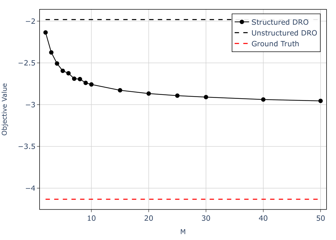
Figure 2. Relaxation gap of the structured DRO problem for different values of $M$ and $\rho$.

The relaxation gap decreases as $M$ increases, corroborating our theoretical findings. The substantial gap between the structured and the unstructured DRO value at $M=50$ when a plateau is reached confirms that (1) is a loose over-approximation of the original nonconvex structured ambiguity set.

5. Conclusions and Outlook

In this paper, we focused on data-driven Wasserstein DRO formulations where the uncertain vector exhibits an i.i.d. structure. By exploiting this structure, we construct a structured ambiguity set that only contains product distributions. To solve the resulting non-convex program, we devise a sequence of convex relaxations that, under mild conditions on the loss function, converge to the optimal solution of the original non-convex problem. Our numerical results certify how structured ambiguity sets can capture uncertainty in a more effective manner than unstructured ambiguity sets, ultimately improving the decision-making task. Future work includes (i) the extension of our lifting procedure to different classes of loss functions besides piecewise and quadratic ones, (ii) the analysis of the relaxation gap for convex loss functions, (iii) addressing the computational burden of data-driven problems where the product empirical distribution is supported on a prohibitive amount of points and extend our analysis to different types of structured dependencies and finally (iv) extending the results to exploit invariance w.r.t. groups $G$ other than the symmetric group $\mathcal{S}_{N}$.

Appendix A Additional Notation

In this appendix we use the following additional notation: By $\operatorname{pr}_{i,j}:X^{N}\times X^{N}\to X\times X$ for $i,j=1,\ldots,N$ we denote the projection onto the $i$-th coordinate in the first factor $X^{N}$ and on the $j$-th coordinate in the second factor $X^{N}$. The projections $\operatorname{pr}_{1:N,1:N}^{M}:X^{M}\times X^{M}\to X^{N}\times X^{N}$, $\operatorname{pr}_{1:N,j}^{M}:X^{M}\times X^{M}\to X^{N}\times X$ are defined similarly. For $P_{1},\ldots,P_{N}\in\mathcal{P}(X)$ we write $\Gamma(P_{1},\ldots,P_{N})$ for all $\Lambda\in\mathcal{P}(X^{N})$ such that $\operatorname{pr}_{i}\#\Lambda=P_{i}$ for $i=1,\ldots,N$. The set $\Gamma(P_{1},\ldots,P_{N})$ is called the set of multi-marginals couplings between $P_{1},\ldots,P_{N}$.

Appendix B Background on measures in Polish spaces

Here we collect some results on measures in Polish spaces. First we note that if $X$ is a Polish space, then so is $\mathcal{P}(X)$ with the topology of weak convergence of measures (i.e. convergence in distribution) [18, 15.15 Theorem]. While $\mathcal{P}_{c}(X)$ is in general not closed as a subset of $\mathcal{P}(X)$, it can be shown that, under the assumptions on the cost $c$ made in Section 2, for $\widehat{P}\in\mathcal{P}_{c}(X)$ the function $\mathcal{P}(X)\to[0,\infty]:P\mapsto W_{c}(P,\widehat{P})$ is lower-semicontinuous in the weak topology and hence Borel measurable [25, Paragraph right after Corollary 2.2.2]. This implies that for each $\rho>0$ and $x_{0}\in X$ the set $\mathcal{P}_{c}(X,\rho)=\{P\mid W_{c}(\delta_{x_{0}},P)\leq\rho\}$ is closed as a subset of $\mathcal{P}(X)$ (and independent of $x_{0}$ because of the weak triangle inequality for $c$) and hence $\mathcal{P}_{c}(X)=\bigcup_{\rho\in\mathbb{N}}\mathcal{P}_{c}(X,\rho)\subseteq\mathcal{P}(X)$ is Borel measurable as a countable union of closed sets. Next, if $c$ is proper (i.e. metric sublevel sets are compact), then, for any $\rho>0$, the set $\mathcal{P}_{c}(X,\rho)$ is compact in the weak topology [35, 25] as is the corresponding Wasserstein ball $\mathbb{B}_{\rho}^{c}(P)$ whenever $P\in\mathcal{P}_{c}(X)$ [35].
Now we turn to mixtures of measures: Since $\mathcal{P}(X)$ is Polish, we can define $\mathcal{P}(\mathcal{P}(X))$ as the set of Borel measures (the Borel $\sigma$-algebra on $\mathcal{P}(X)$ is induced by the weak topology) on $\mathcal{P}(X)$. Now, given any Polish space $Y$ and a Borel subset $A\subseteq Y$ the map $\mathcal{P}(Y)\to[0,1]:P\mapsto P(A)=\int\boldsymbol{1}_{A}\,\text{d}P$ is Borel measurable by [18, 15.13 Theorem]. Hence for any Borel measurable $F:\mathcal{P}(X)\mapsto\mathcal{P}(Y)$ the composition $\mathcal{P}(X)\to[0,1]:P\mapsto F(P)(A)$ is Borel measurable as well. Then for any $\nu\in\mathcal{P}(\mathcal{P}(X))$ the expression $\overline{P}(A):=\int F(P)(A)\,\text{d}\nu(P)$ is well-defined and defines a map from the Borel subsets of $Y$ to $[0,1]$, which is finitely additive. We show that $\overline{P}$ is $\sigma$-continuous from below [14], from which it follows that $\overline{P}$ is countably additive: If $A,A_{i}\subseteq Y$ are Borel such that $A_{i}\nearrow A$ for $i\to\infty$, then $\int F(A_{i})\,\text{d}\nu(P)\nearrow\int F(A)\,\text{d}\nu(P)$ for $i\to\infty$ by the monotone convergence theorem. Hence $\overline{P}$ is a Borel measure and we write $\int F(P)\,\text{d}\nu(P)=\overline{P}$. Furthermore, we often need the following identity that relates the integration w.r.t. a mixture distribution to the integration w.r.t. the mixture measure itself.

Theorem 12.

For any Borel measurable $f:X\to\mathbb{R}$, $\nu\in\mathcal{P}(\mathcal{P}(X))$ and $F:\mathcal{P}(X)\to\mathcal{P}(Y)$ the following holds: $f$ is $\int F(P)\,\text{d}\nu(P)$-integrable iff $f$ is $F(P)$-integrable for $\nu$-almost all $P\in\mathcal{P}(X)$ and in this case

$$\int f\,\text{d}\left(\int F(P)\,\text{d}\nu(P)\right)=\int\left(\int f\,\text{d}(F(P))\right)\,\text{d}\nu(P)\,.$$

Proof.

The map $\kappa:\mathcal{P}(X)\times\mathcal{B}(X)\to[0,1]:(P,A)\mapsto F(P)(A)$ (Here $\mathcal{B}(X)$ denotes the Borel $\sigma$-algebra of $X$) defines a Markov kernel. The claim then follows from [14, 10.2.2. Theorem]. ∎

Appendix C Proofs of Section 2

Proof of Theorem 1..

If $\ell\in\mathcal{G}_{c}$ and $c$ satisfies the weak triangle inequality, then by Lemma 8 it follows that

$$\mathbb{E}_{P}\ell\leq C\mathbb{E}_{P}(1+c(x_{0},\cdot))\leq C(1+\mathbb{E}_{P}c(x_{0},\cdot))\leq C\left(1+\sup_{P\in\mathbb{B}_{\rho}^{c}(\widehat{P})}\int c(x_{0},\cdot)\,\text{d}P\right)<\infty$$

for any $P\in\mathbb{B}_{\rho}^{c}(\widehat{P})$. Now suppose that $c$ is proper, $\ell\in\mathcal{G}_{c}^{<}$ is upper semi-continuous. Since $c$ is proper, $\mathbb{B}_{\rho}^{c}(\widehat{P})\subseteq\mathcal{P}(X)$ is weakly compact. We will show that the map $P\mapsto\mathbb{E}_{P}\ell$ can be uniformly approximated by weakly upper semi-continuous functions on $\mathbb{B}_{\rho}^{c}(\widehat{P})$, which will imply that its restriction to $\mathbb{B}_{\rho}^{c}(\widehat{P})$ is weakly upper semi-continuous and hence attains a maximum. For this purpose, let $\delta\in\mathcal{D}$, $x_{0}\in X$ and $C>0$ as in the definition of $\mathcal{G}_{c}^{<}$. Define for any $r>0$ the function $\ell_{r}=\min\{\ell,C(1+r)\}$. Clearly then for any $x\in X$ it holds that

$$\ell(x)-\ell_{r}(x) \leq\begin{cases}0\,,&c(x_{0},x)\leq r\\ \max\{0,\ell(x)-C(1+r)\}\,,&c(x_{0},x)>r\end{cases}$$

$$\leq\begin{cases}0\,,&c(x_{0},x)\leq r\\ C\delta(c(x_{0},x))\,,&c(x_{0},x)>r\end{cases}\,,$$

where the first follows from $\ell\leq C(1+c(x_{0},\cdot))$ and the second from the stronger $\ell\leq C(1+\delta(c(x_{0},\cdot)))$. Hence if $P\in\mathbb{B}_{\rho}^{c}(\widehat{P})$ it follows for $r\to\infty$ that

$$\lvert\mathbb{E}_{P}\ell-\mathbb{E}_{P}\ell_{r}\rvert\leq\mathbb{E}_{P}\lvert\ell-\ell_{r}\rvert\leq C\int_{c(x_{0},\cdot)>r}\delta(c(x_{0},\cdot))\,\text{d}P$$

$$=C\int_{c(x_{0},\cdot)>r}\frac{\delta(c(x_{0},\cdot))}{c(x_{0},\cdot)}c(x_{0},\cdot)\,\text{d}P\leq C\left(\sup_{\begin{subarray}{c}x\in X\\ c(x_{0},x)>r\end{subarray}}\frac{\delta(c(x_{0},x))}{c(x_{0},x)}\right)\int_{X}c(x_{0},\cdot)\,\text{d}P$$

$$\leq C\underbrace{\left(\sup_{t>r}\frac{\delta(t)}{t}\right)}_{\to 0}\underbrace{\left(\sup_{P\in\mathbb{B}_{\rho}^{c}(\widehat{P})}\int_{X}c(x_{0},\cdot)\,\text{d}P\right)}_{<\infty}\,,$$

with the last claims following from the definition of $\mathcal{D}$ and Lemma 8. Hence the maps $P\mapsto\mathbb{E}_{P}\ell$ can be uniformly approximated by maps of the form $P\mapsto\mathbb{E}_{P}\ell_{r}$ on $\mathbb{B}_{\rho}^{c}(\widehat{P})$. By [18, 15.5 Theorem] the latter maps are weakly upper semi-continuous, which finishes the proof. ∎

Appendix D Proof of Section 3.1

Proof of Theorem 3..

The proof is similar to the proof of Theorem 1. If $\ell\in\widehat{\mathcal{G}}_{c,N}$ and $c$ satisfies the weak triangle inequality, then by Lemma 8 it follows that

$$\mathbb{E}_{P^{\otimes N}}\ell \leq C\mathbb{E}_{x\sim P^{\otimes N}}\prod_{k=1}^{N}(1+c(x_{0},x_{k}))$$

$$\leq C\prod_{k=1}^{N}(1+\mathbb{E}_{x_{k}\sim P}c(x_{0},x_{k}))\leq C\left(1+\sup_{P\in\mathbb{B}_{\rho}^{c}(\widehat{P})}\int c(x_{0},\cdot)\,\text{d}P\right)^{N}$$

for any $P\in\mathbb{B}_{\rho}^{c}(\widehat{P})$. Now suppose that $c$ is proper, $\ell\in\widehat{\mathcal{G}}_{c,N}^{<}$ is upper semi-continuous. Since $c$ is proper, $\mathbb{B}_{\rho}^{c}(\widehat{P})\subseteq\mathcal{P}(X)$ is weakly compact. We will show that the map $P\mapsto\mathbb{E}_{P^{\otimes N}}\ell$ can be uniformly approximated by weakly upper semi-continuous functions on $\mathbb{B}_{\rho}^{c}(\widehat{P})$, which will imply that its restriction to $\mathbb{B}_{\rho}^{c}(\widehat{P})$ is weakly upper semi-continuous and hence attains a maximum. For this purpose, let $\delta\in\mathcal{D}$, $x_{0}\in X$ and $C>0$ as in the definition of $\widehat{\mathcal{G}}_{c,N}^{<}$. Moreover, let $\widehat{C}=\sup_{P\in\mathbb{B}_{\rho}^{c}(\widehat{P})}\int c(x_{0},\widehat{x})\,\text{d}P(\widehat{x})<\infty$, which is finite by Lemma 8. Define for any $r>0$ the function $\ell_{r}:X^{N}\to\mathbb{R}$ by $\ell_{r}(x)=\min\{\ell(x),C(1+r)^{N}\}$ for $x\in X^{N}$. Let $\mathcal{I}=2^{\{1,\ldots,N\}}$ be the power set of $\{1,\ldots,N\}$ and consider for any $r>0$ the following function

$$I_{r}:X^{N}\to\mathcal{I}:x\mapsto\{i\in\{1,\ldots,N\}\mid c(x_{0},x_{i})>r\}\,.$$

Let us partition $X^{N}$ into $X^{N}=\bigsqcup_{I\in\mathcal{I}}I_{r}^{-1}(I)$. Note that each $I_{r}^{-1}(I)$ can be written as $I_{r}^{-1}(I)=X_{I,1}\times\cdots\times X_{I,N}$ with $X_{I,i}=\{x_{i}\in X\mid c(x_{0},x_{i})>r\}$ if $i\in I$ and $X_{I,i}=\{x_{i}\in X\mid c(x_{0},x_{i})\leq r\}$ if $i\notin I$. Now, if $x\in I_{r}^{-1}(I)\cap\{\ell>C(1+r)^{N}\}$, then we have

$$\ell(x)-\ell_{r}(x)$$

$$\leq C\prod_{k=1}^{N}(1+\delta(c(x_{0},x_{k})))-C(1+r)^{N}$$

$$\leq C\left[\prod_{k\in I}(1+\delta(c(x_{0},x_{k})))\prod_{k\notin I}(1+c(x_{0},x_{k}))-(1+r)^{N}\right]$$

$$\leq C\left[\prod_{k\in I}(1+\delta(c(x_{0},x_{k})))\prod_{k\notin I}(1+c(x_{0},x_{k}))-(1+r)^{\lvert I\rvert}\prod_{k\notin I}(1+c(x_{0},x_{k}))\right]$$

$$=C\left[\prod_{k\in I}(1+\delta(c(x_{0},x_{k})))-(1+r)^{\lvert I\rvert}\right]\prod_{k\notin I}(1+c(x_{0},x_{k}))$$

$$\leq C\left[\prod_{k\in I}(1+\delta(c(x_{0},x_{k})))-1\right]\prod_{k\notin I}(1+c(x_{0},x_{k}))\,.$$

On the other hand, if $x\in\{\ell\leq C(1+r)^{N}\}$, then $\ell(x)-\ell_{r}(x)=0$. Note that $I_{r}^{-1}(\emptyset)\subseteq\{\ell\leq C(1+r)^{N}\}$. Integrating w.r.t. $P\in\mathbb{B}_{\rho}^{c}(\widehat{P})$ yields

$$\int_{X^{N}}\ell(x)-\ell_{r}(x)\,\text{d}P^{\otimes N}(x)\leq\sum_{I\in\mathcal{I}}\int_{I_{r}^{-1}(I)}\ell(x)-\ell_{r}(x)\,\text{d}P^{\otimes N}(x)\,.$$

Let us estimate every summand as follows

$$\int_{I_{r}^{-1}(I)}\ell(x)-\ell_{r}(x)\,\text{d}P^{\otimes N}(x)=\int_{I_{r}^{-1}(I)\cap\{\ell>C(1+r)^{N}\}}\ell(x)-\ell_{r}(x)\,\text{d}P^{\otimes N}(x)$$

$$\leq C\int_{I_{r}^{-1}(I)}\left[\prod_{k\in I}(1+\delta(c(x_{0},x_{k})))-1\right]\prod_{k\notin I}(1+c(x_{0},x_{k}))\,\text{d}P^{\otimes N}(x)\,.$$

Let us use the representation $I_{r}^{-1}(I)=X_{I,1}\times\cdots\times X_{I,N}$ to obtain (here $I^{c}$ is the complement of $I$)

$$\int_{I_{r}^{-1}(I)}\left[\prod_{k\in I}(1+\delta(c(x_{0},x_{k})))-1\right]\prod_{k\notin I}(1+c(x_{0},x_{k}))\,\text{d}P^{\otimes N}(x)$$

$$\leq\left(\int_{\prod_{k\in I}X_{I,k}}\left[\prod_{k\in I}(1+\delta(c(x_{0},x_{k})))-1\right]\,\text{d}P^{\otimes\lvert I\rvert}(x_{I})\right)$$

$$\qquad\cdot\left(\int_{\prod_{k\notin I}X_{I,k}}\prod_{k\notin I}(1+c(x_{0},x_{k}))\,\text{d}P^{\otimes\lvert I^{c}\rvert}(x_{I^{c}})\right)$$

$$\leq\left(\int_{\prod_{k\in I}X_{I,k}}\left[\prod_{k\in I}(1+\delta(c(x_{0},x_{k})))-1\right]\,\text{d}P^{\otimes\lvert I\rvert}(x_{I})\right)(1+\widehat{C})^{\lvert I^{c}\rvert}\,.$$

To estimate the first factor, we note that

$$\prod_{k\in I}(1+\delta(c(x_{0},x_{k})))-1=\sum_{J\in 2^{I}\setminus\{\emptyset\}}\prod_{k\in J}\delta(c(x_{0},x_{k}))\,.$$

and that for any $J\in 2^{I}\setminus\{\emptyset\}$ it holds that

$$\int_{\prod_{k\in I}X_{I,k}}\prod_{k\in J}\delta(c(x_{0},x_{k}))\,\text{d}P^{\otimes\lvert I\rvert}(x_{I})=\prod_{k\in J}\int_{X_{I,k}}\delta(c(x_{0},x_{k}))\,\text{d}P(x_{k})$$

and, since $k\in J\subseteq I$, also

$$\int_{X_{I,k}}\delta(c(x_{0},x_{k}))\,\text{d}P(x_{k}) =\int_{c(x_{0},\widehat{x})>r}\frac{\delta(c(x_{0},\widehat{x}))}{c(x_{0},\widehat{x})}c(x_{0},\widehat{x})\,\text{d}P(\widehat{x})$$

$$\leq\left(\sup_{t>r}\frac{\delta(t)}{t}\right)\int c(x_{0},\widehat{x})\,\text{d}P(\widehat{x})$$

$$\leq\widehat{C}\widehat{\delta}(r)\,,$$

where we have defined $\widehat{\delta}(r)=\sup_{t>r}\frac{\delta(t)}{t}$. In all we obtain uniformly for $P\in\mathbb{B}_{\rho}^{c}(\widehat{P})$

$$\lvert\mathbb{E}_{P^{\otimes N}}\ell-\mathbb{E}_{P^{\otimes N}}\ell_{r}\rvert \leq\int_{X^{N}}\ell(x)-\ell_{r}(x)\,\text{d}P^{\otimes N}(x)$$

$$\leq C\sum_{I\in\mathcal{I}}\left((1+\widehat{C})^{N-\lvert I\rvert}\sum_{J\in 2^{I}\setminus\{\emptyset\}}\widehat{C}^{\lvert J\rvert}\widehat{\delta}(r)^{\lvert J\rvert}\right)\,,$$

and the right hand side converges to $0$ as $r\to\infty$, since $\delta\in\mathcal{D}$. Hence the maps $P\mapsto\mathbb{E}_{P}\ell$ can be uniformly approximated by maps of the form $P\mapsto\mathbb{E}_{P}\ell_{r}$ on $\mathbb{B}_{\rho}^{c}(\widehat{P})$. By [18, 15.5 Theorem] the latter maps are weakly upper semi-continuous, which finishes the proof. ∎

Proof of Lemma 1..

Let $P\in\mathbb{B}_{\rho}^{c}(\widehat{P})$. Then $W_{c}(P,\widehat{P})\leq\rho$ and by Lemma 15 it follows that $W_{c^{N}}(P^{\otimes N},\widehat{P}^{\otimes N})\leq N\rho$. Hence $P^{\otimes N}\in\mathbb{B}_{N\rho}^{c^{N}}(\widehat{P}^{\otimes N})$. ∎

Appendix E Proofs of Section 3.2

Proof of Theorem 4..

We have

(36) $$\begin{gathered}\operatorname{U}(\ell_{\operatorname{sym}})=\sup_{\overline{P}\in\mathbb{B}_{N\rho}^{c^{N}}(P^{\otimes N})}\frac{1}{N!}\sum_{\pi\in\mathcal{S}_{N}}\int\ell\circ\pi\,\text{d}\overline{P}=\sup_{\overline{P}\in\mathbb{B}_{N\rho}^{c^{N}}(P^{\otimes N})}\frac{1}{N!}\sum_{\pi\in\mathcal{S}_{N}}\int\ell\,\text{d}\pi\#\overline{P}\\ =\sup_{\overline{P}\in\mathbb{B}_{N\rho}^{c^{N}}(P^{\otimes N})}\int\ell\,\text{d}\overline{P}_{\operatorname{sym}}=\sup_{\overline{P}\in\mathbb{B}_{N\rho}^{c^{N}}(P^{\otimes N})_{\operatorname{sym}}}\int\ell\,\text{d}\overline{P}\,,\end{gathered}$$

where the first equality follows by the definition of the symmetrization of a function $\ell$ and the linearity of the integral, the second equality from the pushforward identity of the Lebesgue integral and the last equality from the linearity of the integral in the measure and the definition (18). Now, to see (20), we first note that $\supseteq$ trivially holds, since for any $\overline{P}\in\mathbb{B}_{N\rho}^{c^{N}}(\widehat{P}^{\otimes N})\cap\mathcal{P}_{\operatorname{sym}}(X^{N})$ we have $\overline{P}_{\operatorname{sym}}=\overline{P}$. To see $\subseteq$, pick any $\overline{P}\in\mathbb{B}_{N\rho}^{c^{N}}(\widehat{P}^{\otimes N})$. Let $\epsilon>0$ be arbitrary and let $\Lambda\in\Gamma(\overline{P},\widehat{P}^{\otimes N})$ be a coupling such that $\int c^{N}\,\text{d}\Lambda\leq N\rho+\epsilon$. Then by Lemma 9 there exists some $\Lambda_{\operatorname{sym}}\in\Gamma(\overline{P}_{\operatorname{sym}},\widehat{P}^{\otimes N})$ with $\int c^{N}\,\text{d}\Lambda_{\operatorname{sym}}\leq N\rho+\epsilon$. Since $\epsilon>0$ was arbitrary, it follows that $\overline{P}_{\operatorname{sym}}\in\mathbb{B}_{N\rho}^{c^{N}}(P^{\otimes N})$. ∎

Appendix F Proofs of Section 3.4

Proof of Lemma 4.

(i) Since $c$ is proper, so is $c^{M}$ and thus $\mathbb{B}_{M\rho}^{c^{M}}(\widehat{P}^{\otimes M})$ is weakly compact. Hence $\mathbb{B}_{M\rho}^{c^{M}}(\widehat{P}^{\otimes M})_{\operatorname{sym}}=\mathbb{B}_{M\rho}^{c^{M}}(\widehat{P}^{\otimes M})\cap\mathcal{P}_{\operatorname{sym}}(X^{M})$ is, as an intersection of a weakly compact and weakly closed set, itself weakly compact. Then $\mathcal{U}_{M}$, being the compact image of the latter set under the weakly continuous map $\overline{P}\mapsto\operatorname{pr}_{1:N}^{M}\#\overline{P}$ is weakly compact.
(ii) It suffices to show that $\mathcal{W}\subseteq\mathcal{U}_{M}$ and that $\mathcal{U}_{M}$ is convex. The latter follows from the convexity of $\mathbb{B}_{M\rho}^{c^{M}}(\widehat{P}^{\otimes M})_{\operatorname{sym}}$ and the former from the fact that $\operatorname{pr}_{1:N}^{M}\#P^{\otimes M}=P^{\otimes N}$ with $P^{\otimes M}\in\mathbb{B}_{M\rho}^{c^{M}}(\widehat{P}^{\otimes M})_{\operatorname{sym}}$ for all $P\in\mathbb{B}_{\rho}^{c}(\widehat{P})$ by Lemma 1.
(iii) Let $\widetilde{P}\in\mathcal{U}_{M+1}$. Then $\widehat{P}=\operatorname{pr}_{1:N}^{M}\#\overline{P}^{\prime}$ for some $\overline{P}^{\prime}\in\mathbb{B}_{(M+1)\rho}^{c^{M+1}}(\widehat{P}^{\otimes(M+1)})_{\operatorname{sym}}$. Since $\overline{P}^{\prime},\widehat{P}^{\otimes(M+1)}\in\mathcal{P}_{\operatorname{sym}}(X^{M+1})$, by Lemma 9 there exists a $\widehat{\Lambda}\in\widehat{\Gamma}_{\operatorname{sym}}(\widehat{P}^{\otimes(M+1)},\overline{P}^{\prime})$ such that $\int c^{M+1}\,\text{d}\widehat{\Lambda}=W_{c^{M+1}}(\widehat{P}^{\otimes(M+1)},\overline{P}^{\prime})\leq(M+1)\rho$.
Consider $\Lambda=\operatorname{pr}_{1:M,1:M}^{M+1,M+1}\#\widehat{\Lambda}\in\Gamma(\widehat{P}^{\otimes M},\overline{P})$ with $\overline{P}=\operatorname{pr}_{1:M}^{M+1}\#\overline{P}^{\prime}$. We claim that $\int c^{M}\,\text{d}\Lambda\leq M\rho$. For this purpose we note that $\int c\circ\operatorname{pr}_{1,1}\,\text{d}\widehat{\Lambda}\leq\rho$. Indeed,

$$(M+1)\rho\geq\int c^{M+1}\,\text{d}\widehat{\Lambda}=\sum_{i=1}^{M+1}\int c\circ\operatorname{pr}_{i,i}\,\text{d}\widehat{\Lambda}=(M+1)\int c\circ\operatorname{pr}_{1,1}\,\text{d}\widehat{\Lambda}\,,$$

where the first equality follows from $c^{M+1}=\sum_{i=1}^{M+1}c\circ\operatorname{pr}_{i,i}$ and the last equality follows from $\widehat{\Lambda}$ being a symmetric coupling. Then

$$\int c^{M}\,\text{d}\Lambda=\int c^{M}\circ\operatorname{pr}_{1:M,1:M}^{M+1,M+1}\,\text{d}\widehat{\Lambda}=\sum_{i=1}^{M}\int c\circ\operatorname{pr}_{i,i}\,\text{d}\widehat{\Lambda}=M\int c\circ\operatorname{pr}_{1,1}\,\text{d}\widehat{\Lambda}\leq M\rho\,.$$

Thus we have shown that $W_{c^{M}}(\widehat{P}^{\otimes M},\overline{P})\leq M\rho$, or equivalently $\overline{P}\in\mathbb{B}_{M\rho}^{c^{M}}(\widehat{P}^{\otimes M})_{\operatorname{sym}}$. But then $\widetilde{P}=\operatorname{pr}_{1:N}^{M+1}\#\overline{P}^{\prime}=\operatorname{pr}_{1:N}^{M}\#\operatorname{pr}_{1:M}^{M+1}\#\overline{P}^{\prime}=\operatorname{pr}_{1:N}^{M}\#\overline{P}$ since $\operatorname{pr}_{1:N}^{M+1}\circ\operatorname{pr}_{1:M}^{M}=\operatorname{pr}_{1:N}^{M+1}$ if $M\geq N$. Additionally, it is easily verified that $\overline{P}$ is symmetric, just because $\overline{P}^{\prime}$ is. Hence, by the definition of $\mathcal{U}_{M}$, we have $\widetilde{P}\in\mathcal{U}_{M}$. ∎

Proof of Theorem 5..

We have already noted that $\widehat{\operatorname{U}}_{\infty}^{\operatorname{sym}}(\ell)\leq\operatorname{U}_{\infty}^{\operatorname{sym}}(\ell)$. Moreover, in the proof of Theorem 1 is it shown that if $\ell$ is upper semi-continuous and $\ell\in\mathcal{G}_{c^{N}}^{<}(X^{N})$, then $\overline{P}\mapsto\mathbb{E}_{\overline{P}}\ell$ is weakly upper semi-continuous on $\mathbb{B}_{N\rho}^{c^{N}}(\widehat{P}^{\otimes N})$. Then pick for each $M\geq N$ some $\overline{P}_{M}\in\mathcal{U}_{M}$ such that

$$\mathbb{E}_{x\sim\overline{P}_{M}}\ell(x)\geq\sup_{\overline{P}\in\mathcal{U}_{M}}\mathbb{E}_{x\sim\overline{P}}\ell(x)-\frac{1}{M}=\operatorname{U}_{M}^{\operatorname{sym}}(\ell)-\frac{1}{M}\,.$$

Then, since $\mathcal{U}_{M+1}\subseteq\mathcal{U}_{M}$ for all $M\geq N$ by Lemma 4, it follows that $\overline{P}_{M}\in\mathcal{U}_{L}$ for any $N\leq L\leq M$. Moreover, by the same Lemma each $\mathcal{U}_{M}$ is weakly compact and thus there exists a subsequence $\overline{P}_{M_{k}}$ and $\overline{P}\in\bigcap_{M\geq N}\mathcal{U}_{M}=\mathcal{U}_{\infty}$ such that $\overline{P}_{M_{k}}\to\overline{P}$ weakly for $k\to\infty$. But then

$$\begin{gathered}\widehat{\operatorname{U}}_{\infty}^{\operatorname{sym}}(\ell)\geq\mathbb{E}_{x\sim\overline{P}}\ell(x)\geq\limsup_{k\to\infty}\mathbb{E}_{x\sim\overline{P}_{M_{k}}}\ell(x)\geq\limsup_{k\to\infty}\left(\operatorname{U}_{M_{k}}^{\operatorname{sym}}(\ell)-\frac{1}{M_{k}}\right)\\ \geq\limsup_{k\to\infty}\operatorname{U}_{M_{k}}^{\operatorname{sym}}(\ell)-\limsup_{k\to\infty}\frac{1}{M_{k}}=\operatorname{U}_{\infty}^{\operatorname{sym}}(\ell)\,,\end{gathered}$$

where the last inequality holds because $\limsup_{k}(a_{k}+b_{k})\leq\limsup_{k}a_{k}+\limsup_{k}b_{k}$ for any two real sequences $(a_{k})_{k=1}^{\infty}$ and $(b_{k})_{k=1}^{\infty}$. ∎

Proof of Lemma 5..

First we show $\supseteq$. If $\overline{P}\in\widehat{\mathcal{W}}_{\infty}$, then we claim that
$\operatorname{pr}_{1:N}\#\overline{P}\in\mathcal{U}_{M}$ for all $M\geq N$. Indeed, it holds that $\operatorname{pr}_{1:N}\#\overline{P}=\operatorname{pr}_{1:N}\#(\operatorname{pr}_{1:M}\#\overline{P})$ and $\operatorname{pr}_{1:M}\#\overline{P}\in\mathbb{B}_{M\rho}^{c^{M}}(\widehat{P}^{\otimes M})$ by the definition of $\widehat{\mathcal{W}}_{\infty}$. Moreover, $\operatorname{pr}_{1:M}\#\overline{P}$ is symmetric, since $\overline{P}$ is symmetric. Hence, $\operatorname{pr}_{1:N}\#\overline{P}\in\mathcal{U}_{M}$ follows by the definition of $\mathcal{U}_{M}$. Now we will show that $\subseteq$ holds. For this purpose let $\widetilde{P}\in\mathcal{U}_{M}$ for all $M\geq N$. Then for each $M\geq N$ there exists some $\overline{P}_{M}\in\mathbb{B}_{M\rho}^{c^{M}}(\widehat{P}^{\otimes M})_{\operatorname{sym}}$ such that $\widetilde{P}=\operatorname{pr}_{1:N}\overline{P}_{M}$. We have to exhibit a single $\overline{P}\in\mathcal{P}_{\operatorname{sym}}(X^{\infty})$ such that $\widetilde{P}=\operatorname{pr}_{1:N}\#\overline{P}$ and $\operatorname{pr}_{1:M}\#\overline{P}\in\mathbb{B}_{M\rho}^{c^{M}}(\widehat{P}^{\otimes M})$ for all $M\geq 1$. For that purpose we notice first that if $\overline{P}_{M}\in\mathbb{B}_{M\rho}^{c^{M}}(\widehat{P}^{\otimes M})_{\operatorname{sym}}$, then for all $1\leq L\leq M$ it holds that $\operatorname{pr}_{1:L}\#\overline{P}_{M}\in\mathbb{B}_{L\rho}^{c^{L}}(\widehat{P}^{\otimes L})_{\operatorname{sym}}$. Indeed, symmetry is clear from the symmetry of $\overline{P}_{M}$. To see why $\operatorname{pr}_{1:L}\#\overline{P}_{M}\in\mathbb{B}_{L\rho}^{c^{L}}(\widehat{P}^{\otimes L})$, let $\widehat{\Lambda}\in\Gamma_{\operatorname{sym}}(\widehat{P}^{\otimes M},\overline{P}_{M})$ be a coupling (see Lemma 9) such that $\int c^{M}\,\text{d}\widehat{\Lambda}=W_{c^{M}}(\widehat{P}^{\otimes M},\overline{P}_{M})\leq M\rho$. Just as in the proof of Lemma 4 one can show, by exploiting symmetry of $\widehat{\Lambda}$, that the coupling $\Lambda=\operatorname{pr}_{1:L,1:L}^{M,M}\#\widehat{\Lambda}$ satisfies $\Lambda\in\Gamma_{\operatorname{sym}}(\widehat{P}^{\otimes L},\operatorname{pr}_{1:L}\#\overline{P}_{M})$ and that $\int c^{L}\,\text{d}\Lambda\leq L\rho$, i.e. $\operatorname{pr}_{1:L}\#\overline{P}_{M}\in\mathbb{B}_{L\rho}^{c^{L}}(\widehat{P}^{\otimes L})$. Thus we have established that any $\overline{P}_{M}\in\mathbb{B}_{M\rho}^{c^{M}}(\widehat{P}^{\otimes M})_{\operatorname{sym}}$ can be projected down to $\operatorname{pr}_{1:L}^{M}\#\overline{P}_{M}\in\mathbb{B}_{L\rho}^{c^{L}}(\widehat{P}^{\otimes L})_{\operatorname{sym}}$. Let us denote $\boldsymbol{P}^{M}=\{\overline{P}^{\prime}\in\mathbb{B}_{M\rho}^{c^{M}}(\widehat{P}^{\otimes M})_{\operatorname{sym}}\mid\operatorname{pr}_{1:N}\#\overline{P}^{\prime}=\widetilde{P}\}$ and define now the maps $\phi_{M,L}:\boldsymbol{P}^{M}\to\boldsymbol{P}^{L}:\overline{P}^{\prime}\mapsto\operatorname{pr}_{1:L}^{M}\#\overline{P}^{\prime}$ for $N\leq L\leq M$. Then, since $\phi_{M,K}=\phi_{L,K}\circ\phi_{M,L}$ and $\phi_{M,M}=\operatorname{id}_{\boldsymbol{P}^{M}}$ for all $N\leq K\leq L\leq M$, the family $\{(\boldsymbol{P}^{M})_{M\geq N},(\phi_{M,L})_{M\geq L\geq N}\}$ is projective [34]. Hence we can form the projective limit

$$\varprojlim_{M\geq N}\boldsymbol{P}^{M}=\{(\overline{P}_{M}^{\prime})_{M\geq N}\in\boldsymbol{P}\mid\phi_{M,L}(\overline{P}_{M}^{\prime})=\overline{P}_{L}^{\prime}\}\subseteq\boldsymbol{P}\,,$$

where $\boldsymbol{P}=\prod_{M\geq N}\boldsymbol{P}^{M}$ is nonempty, since $(\overline{P}_{M})_{M\geq N}\in\boldsymbol{P}$. Since each $\boldsymbol{P}^{M}$ is Hausdorff and weakly compact, by [34, Theorem 29.11] the set $\varprojlim_{M\geq N}\boldsymbol{P}^{M}$ is nonempty. Let $(\overline{P}_{M}^{\prime})_{M\geq N}\in\varprojlim_{M\geq N}\boldsymbol{P}^{M}$ be arbitrary. By the very definition of $\varprojlim_{M\geq N}\boldsymbol{P}^{M}$ it follows that the family $(X^{M},\overline{P}_{M}^{\prime})_{M\geq N}$ is consistent in the sense of Kolmogorov. By the Kolmogorov extension theorem [18, 15.27 Corollary] there exists a single Borel probability measure $\overline{P}\in\mathcal{P}(X^{\infty})$ such that $\operatorname{pr}_{1:M}\#\overline{P}=\overline{P}_{M}^{\prime}\in\mathbb{B}_{M\rho}^{c^{M}}(\widehat{P}^{\otimes M})$ for all $M\geq N$. Since each $\overline{P}_{M}^{\prime}$ is symmetric, so is $\overline{P}$. Moreover, clearly for $N=M$ it follows from the definition of $\boldsymbol{P}^{N}$ that $\operatorname{pr}_{1:N}\#\overline{P}=\widetilde{P}$. Hence we have exhibited the desired distribution $\overline{P}$, which shows that $\widetilde{P}\in\mathcal{U}_{\infty}$. ∎

Before we proceed to the proof of Theorem 6 we need to establish the following result that is of independent interest.

Theorem 13.

Let $c:X\times X\to[0,\infty)$ be a proper transportation cost, $\nu\in\mathcal{P}(\mathcal{P}(X))$ and $\widehat{P}\in\mathcal{P}_{c}(X)$. Then

(37) $$\sup_{M\in\mathbb{N}}\frac{1}{M}W_{c^{M}}\left(\int_{\mathcal{P}(X)}P^{\otimes M}\,\text{d}\nu(P),\widehat{P}^{\otimes M}\right)=\int W_{c}(P,\widehat{P})\,\text{d}\nu(P)\,.$$

Proof.

First we show “$\leq$”. Let $M\in\mathbb{N}$ be fixed. Then, by [33, Theorem 4.8], it holds that

$$W_{c^{M}}\left(\int_{\mathcal{P}(X)}P^{\otimes M}\,\text{d}\nu(P),\widehat{P}^{\otimes M}\right) \leq\int_{\mathcal{P}(X)}W_{c^{M}}\left(P^{\otimes M},\widehat{P}^{\otimes M}\right)\,\text{d}\nu(P)$$

$$=M\int_{\mathcal{P}(X)}W_{c}(P,\widehat{P})\,\text{d}\nu(P)$$

where in the equality we have used the fact that $W_{c^{M}}\left(\widetilde{P}^{\otimes M},P^{\otimes M}\right)=MW_{c}(\widetilde{P},P)$, established in Lemma 15. Dividing by $M$ and taking $\sup_{M\in\mathbb{N}}$ on both sides yields “$\leq$”. The argument for “$\geq$” is a bit more involved. Define $\overline{P}_{M}:=\int_{\mathcal{P}(X)}P^{\otimes M}\,\text{d}\nu(P)$ for $M\in\mathbb{N}$. It is sufficient to show for each $\rho>0$ that

(38) $$\left[\forall M\in\mathbb{N}\;:\;W_{c^{M}}\left(\overline{P}_{M},\widehat{P}^{\otimes M}\right)\leq M\rho\right]\Longrightarrow\int_{\mathcal{P}(X)}W_{c}(P,\widehat{P})\,\text{d}\nu(P)\leq\rho\,.$$

Indeed, if (38) is true and $<$ holds in (37), then by picking $\rho$ that is larger than the left hand side in (37) and smaller than the right hand side in (37) and applying (38) we get a contradiction. In the following we will thus show (38). Firs fix $\rho>0$ and assume that the left side of (38) holds. We will show that the right hand side of (38) holds in steps.
Step 1. (Construction of a single coupling $\Lambda$). Define for each $M\in\mathbb{N}$ the following set

$$\boldsymbol{\Gamma}^{M}=\left\{\widehat{\Lambda}\in\Gamma_{\operatorname{sym}}(\overline{P}_{M},\widehat{P}^{\otimes M})\;\middle|\;\int_{X^{M}\times X^{M}}c^{M}\,\text{d}\widehat{\Lambda}\leq M\rho\right\}\subseteq\mathcal{P}(X^{M}\times X^{M})\,.$$

Then, by Lemma 2, for each $M\in\mathbb{N}$ it holds that $\boldsymbol{\Gamma}^{M}\neq\emptyset$. Moreover, the set $\boldsymbol{\Gamma}^{M}$ is weakly compact, since it can be written as

$$\boldsymbol{\Gamma}^{M}=\Gamma(\overline{P}_{M},P^{\otimes M})\cap\mathcal{P}_{\operatorname{sym}}(X^{M}\times X^{M})\cap\left\{\widehat{\Lambda}\in\mathcal{P}(X^{M}\times X^{M})\mid\int c^{M}\,\text{d}\widehat{\Lambda}\leq M\rho\right\}$$

with $\mathcal{P}_{\operatorname{sym}}(X^{M}\times X^{M})$ being the set of measures $\Lambda\in\mathcal{P}(X^{M}\times X^{M})$ with $(\pi\oplus\pi)\#\Lambda=\Lambda$ for all $\pi\in\mathcal{S}_{M}$. By [33, Lemma 4.4, Proof of Theorem 4.1] the set $\Gamma(\overline{P}_{M},P^{\otimes M})$ is weakly compact and the latter two sets are weakly closed, from which weak compactness of $\boldsymbol{\Gamma}^{M}$ follows. Define the (nonempty) product set

$$\boldsymbol{\Gamma}={\prod}_{M=1}^{\infty}\boldsymbol{\Gamma}^{M}\,.$$

As in the proof of Lemma 4, for each $M,L\in\mathbb{N}$ with $L\leq M$ define the maps

$$\phi_{M,L}:\boldsymbol{\Gamma}^{M}\to\boldsymbol{\Gamma}^{L}:\widehat{\Lambda}\mapsto(\operatorname{pr}_{1:L,1:L}^{M,M})\#\widehat{\Lambda}\,.$$

The fact that $\phi_{M,L}$ are well-defined can be verified by the same computation as in Lemma 4 and by exploiting the symmetry of each coupling in $\boldsymbol{\Gamma}^{M}$. Moreover, the family $\{(\boldsymbol{\Gamma}^{M})_{M\in\mathbb{N}},(\phi_{M,L})_{M\geq L}\}$ is projective, i.e., it holds that $\phi_{M,N}=\phi_{L,N}\circ\phi_{M,L}$ for all $N\leq L\leq M$ as well as $\phi_{M,M}=\operatorname{id}_{\boldsymbol{\Gamma}^{M}}$. Hence we can form the projective limit

$$\varprojlim_{M}\boldsymbol{\Gamma}^{M}:=\{(\widehat{\Lambda}_{M})_{M\in\mathbb{N}}\in\boldsymbol{\Gamma}\mid\phi_{M,L}(\widehat{\Lambda}_{M})=\widehat{\Lambda}_{L}\text{\ for all\ }L\leq M\,,\;M,L\in\mathbb{N}\}\,.$$

Since each $\boldsymbol{\Gamma}^{M}$ is compact and Hausdorff, the set $\varprojlim_{M}\boldsymbol{\Gamma}^{M}$ is nonempty by [34, Theorem 29.11] and we can pick some $(\Lambda_{M})_{M\in\mathbb{N}}\in\varprojlim_{M}\boldsymbol{\Gamma}^{M}$. By the very definition of $\varprojlim_{M}\boldsymbol{\Gamma}^{M}$ it follows that (if we see each $\Lambda_{M}$ as a probability measure on $(X\times X)^{M}\cong X^{M}\times X^{M}$) the family $((X\times X)^{M},\Lambda_{M})_{M\in\mathbb{N}}$ is consistent in the sense of Kolmogorov. By the Kolmogorov extension theorem [18, 15.27 Corollary] there exists a single Borel probability measure $\Lambda\in\mathcal{P}(X^{\infty}\times X^{\infty})$ such that $\phi_{M}(\Lambda):=\operatorname{pr}_{1:M,1:M}\#\Lambda=\Lambda_{M}$ for each $M\in\mathbb{N}$. Then $\Lambda$ is symmetric, since each $\Lambda_{M}$ is. We claim that $\Lambda\in\Gamma(\overline{P},\widehat{P}^{\otimes\infty})$ with $\overline{P}=\int P^{\otimes\infty}\,\text{d}\nu(P)$. Indeed, for each $M\in\mathbb{N}$ it holds that $\operatorname{pr}_{1:M,\emptyset}\#\Lambda=\overline{P}_{M}$ and $\operatorname{pr}_{\emptyset,1:M}\#\Lambda=P^{\otimes M}$. Then, evaluation of the marginals $\operatorname{pr}_{1:\infty,\emptyset}\#\Lambda$ and $\operatorname{pr}_{\emptyset,1:\infty}\#\Lambda$ on the finite cylinder sets of the Borel $\sigma$-algebra on $X^{\infty}$ yields the claim. In summary we have obtained a symmetric coupling $\Lambda\in\Gamma_{\operatorname{sym}}(\overline{P},\widehat{P}^{\otimes\infty})$ on the countable Cartesian product $X^{\infty}\times X^{\infty}$ such that

(39) $$\int_{X^{\infty}\times X^{\infty}}c^{M}\circ\operatorname{pr}_{1:M,1:M}\,\text{d}\Lambda\leq M\rho\text{\ \ for all\ \ }M\in\mathbb{N}\,.$$

Step 2. (Construction of a family of couplings between $\widehat{P}$ and $P$). Now we will construct couplings between $\widehat{P}$ and $P$ for $P\in\mathcal{P}(X)$. For this purpose let $\Lambda(\cdot\mid\cdot)$ denote the disintegration kernel of $\Lambda$ w.r.t. the first marginal $\overline{P}$, i.e. $\Lambda(\cdot\mid\eta)\in\mathcal{P}(X^{\infty})$ for $\overline{P}$-a.a. $\eta\in X^{\infty}$, the map $X^{\infty}\to[0,1]:\eta\mapsto\Lambda(A\mid\eta)$ is Borel-measurable for each Borel set $A\subseteq X^{\infty}$ and

(40) $$\Lambda(A\times B)=\int_{A}\Lambda(B\mid\eta)\,\text{d}\overline{P}(\eta)\text{\ \ for any Borel sets $A,B\subseteq X^{\infty}$}\,.$$

Such a disintegration kernel exists according to [22, Theorem 8.36], since $X^{\infty}$ is Polish.
Step 2.1 (Symmetry of disintegration kernel). For this disintegration kernel the following identity holds:

(41) $$\pi\#\Lambda(\cdot\mid\eta)=\Lambda(\cdot\mid\pi(\eta))\text{\ \ for all $\pi\in\mathcal{S}_{\infty}$ and $\overline{P}$-a.a.\ }\eta\in X^{\infty}\,.$$

Indeed, let $A,B\subseteq X^{\infty}$ be Borel. Then by symmetry of $\Lambda$ and $\overline{P}$ it follows

$$\int_{A}(\pi\#\Lambda)(B\mid\eta)\,\text{d}\overline{P}(\eta)$$

$$\qquad=\int_{A}\Lambda(\pi^{-1}(B)\mid\eta)\,\text{d}\overline{P}(\eta)=\Lambda(A\times\pi^{-1}(B))=\Lambda(\pi(A)\times B)$$

$$\qquad=\int_{\pi(A)}\Lambda(B\mid\eta)\,\text{d}\overline{P}(\eta)=\int_{X^{\infty}}\boldsymbol{1}_{A}(\pi^{-1}(\eta))\Lambda(B\mid\pi^{-1}(\pi(\eta)))\,\text{d}\overline{P}(\eta)$$

$$\qquad=\int_{A}\Lambda(B\mid\pi(\eta))\,\text{d}\overline{P}(\eta)\,.$$

Hence (41) is established.
Step 2.2 ($P^{\infty}$-integral of disintegration kernel). Now, for each $P\in\mathcal{P}(X)$ define a Borel probability measure on $X^{\infty}\times X^{\infty}$ by

(42) $$\Lambda(A\times B\mid P^{\otimes\infty}):=\int_{A}\Lambda(B\mid\eta)\,\text{d}P^{\otimes\infty}(\eta)\text{\ \ for Borel\ \ }A,B\subseteq X^{\infty}\,.$$

It then holds by definition of $\Lambda(\cdot\mid P^{\otimes\infty})$ that

$$\Lambda(A\times X^{\infty}\mid P^{\otimes\infty})=P^{\otimes\infty}(A)\text{\ \ for all Borel\ \ }A\subseteq X^{\infty}\,,$$

and hence $\Lambda(\cdot\mid P^{\otimes\infty})\in\Gamma(P^{\otimes\infty},\cdot)$, i.e. the first marginal of $\Lambda(\cdot\mid P^{\otimes\infty})$ is $P^{\otimes\infty}$.
Step 2.3 (Second marginal of $\Lambda(\cdot\mid P^{\otimes\infty})$). Now we will show that the second marginal of $\Lambda(\cdot\mid P^{\otimes\infty})$ is actually $\widehat{P}^{\otimes\infty}$ for $\nu$-a.a. $P\in\mathcal{P}(X)$, i.e. that $\Lambda(X^{\infty}\times B\mid P^{\otimes\infty})=\widehat{P}^{\otimes\infty}(B)$ for all $\nu$-a.a. $P\in\mathcal{P}(X)$ and Borel sets $B\subseteq X^{\infty}$.
Step 2.3.1 (Averaged second marginal of $\Lambda(\cdot\mid P^{\otimes\infty})$) First we note that

$$\int\Lambda(X^{\infty}\times B\mid P^{\otimes\infty})\,\text{d}\nu(P) =\int\int_{X^{\infty}}\Lambda(B\mid\eta)\,\text{d}P^{\otimes\infty}(\eta)\,\text{d}\nu(P)$$

$$=\int_{X^{\infty}}\Lambda(B\mid\eta)\,\text{d}\overline{P}(\eta)$$

$$=\Lambda(X^{\infty}\times B)$$

$$=\widehat{P}^{\otimes\infty}(B)$$

for all Borel sets $B\subseteq X^{\infty}$, where the third equality is due to Theorem 12 and the definition of $\overline{P}$ and the fourth equality due to (40). This shows that the averaged second marginal of $\Lambda(\cdot\mid P^{\otimes\infty})$ is $\widehat{P}^{\otimes\infty}$.
Step 2.3.2 (Symmetry of second marginal of $\Lambda(\cdot\mid P^{\otimes\infty})$). Let us first show that the measure $B\mapsto\Lambda(X^{\infty}\times B\mid P^{\otimes\infty})=:\widehat{\Lambda}(B\mid P^{\otimes\infty})$ (i.e. the second marginal of $\Lambda(\cdot\mid P^{\otimes\infty})$) on $X^{\infty}$ is symmetric for $\nu$-a.a. $P\in\mathcal{P}(X)$. To this end let $\pi\in\mathcal{S}_{\infty}$ and $B\subseteq X^{\infty}$ Borel. Then it holds for $\nu$-a.a. $P$ that

$$\widehat{\Lambda}(\pi^{-1}(B)\mid P^{\otimes\infty}) =\int_{X^{\infty}}\Lambda(\pi^{-1}(B)\mid\eta)\,\text{d}P^{\otimes\infty}(\eta)$$

$$=\int_{X^{\infty}}\Lambda(B\mid\pi(\eta))\,\text{d}P^{\otimes\infty}(\eta)$$

$$=\int_{X^{\infty}}\Lambda(B\mid\eta)\,\text{d}P^{\otimes\infty}(\eta)$$

$$=\widehat{\Lambda}(B\mid P^{\otimes\infty})\,,$$

since $\Lambda(\pi^{-1}(B)\mid\eta)=\Lambda(B\mid\pi(\eta))$ holds for $\overline{P}$-a.a. $\eta\in X^{\infty}$ by (41) and hence also for $P^{\otimes\infty}$-a.a. $\eta\in X^{\infty}$ for $\nu$-a.a. $P\in\mathcal{P}(X)$. In summary we now know that $\widehat{\Lambda}(\cdot\mid P^{\otimes\infty})$ is symmetric for $\nu$-a.a. $P$ and that

(43) $$\int\widehat{\Lambda}(\cdot\mid P^{\otimes\infty})\,\text{d}\nu(P)=\widehat{P}^{\otimes\infty}\,.$$

By [20, Theorem 5.3] the extreme points of $\mathcal{P}_{\operatorname{sym}}(X^{\infty})$ are precisely the measures of the form $\widetilde{P}^{\otimes\infty}$ with $\widetilde{P}\in\mathcal{P}(X)$. Hence from (43) and Lemma 14 (taking there $Y=\mathcal{P}(X)$, $Z=\mathcal{P}(X^{\infty})$, $\mathscr{Z}=\mathcal{P}_{\operatorname{sym}}(X^{\infty})$, $F(P)=\widehat{\Lambda}(\cdot\mid P^{\otimes\infty})$) we conclude that $\widehat{\Lambda}(\cdot\mid P^{\otimes\infty})=\widehat{P}^{\otimes\infty}$ and thus $\Lambda(\cdot\mid P^{\otimes\infty})\in\Gamma_{\operatorname{sym}}(P^{\otimes\infty},\widehat{P}^{\otimes\infty})$ for $\nu$-a.a. $P$, i.e. the second marginal of $\Lambda(\cdot\mid P^{\otimes\infty})$ is $\widehat{P}^{\otimes\infty}$.
Step 2.4 (Construction of a family of couplings using $\Lambda(\cdot\mid P^{\otimes\infty})$). Finally define the family of couplings

(44) $$\Lambda(\cdot\mid P):=\operatorname{pr}_{1,1}\#\Lambda(\cdot\mid P^{\otimes\infty})\in\Gamma(P,\widehat{P})\text{\ \ for $\nu$-a.a. $P$}\,.$$

Step 3. (Conclusion of right hand side of of (38)). By unfolding all definitions we obtain finally

$$\int_{\mathcal{P}(X)}W_{c}(P,\widehat{P})\,\text{d}\nu(P) \leq\int_{\mathcal{P}(X)}\int_{X\times X}c\,\text{d}\Lambda(\cdot\mid P)\,\text{d}\nu(P)$$

$$=\int_{\mathcal{P}(X)}\int_{X^{\infty}\times X^{\infty}}c\circ\operatorname{pr}_{1,1}\,\text{d}\Lambda(\cdot\mid P^{\otimes\infty})\,\text{d}\nu(P)$$

$$=\int_{\mathcal{P}(X)}\int_{X^{\infty}}\int_{X^{\infty}}c\circ\operatorname{pr}_{1,1}(\eta,\xi)\,\text{d}\Lambda(\xi\mid\eta)\,\text{d}P^{\otimes\infty}(\eta)\,\text{d}\nu(P)$$

$$=\int_{X^{\infty}}\int_{X^{\infty}}c\circ\operatorname{pr}_{1,1}(\eta,\xi)\,\text{d}\Lambda(\xi\mid\eta)\,\text{d}\overline{P}(\eta)$$

$$=\int_{X^{\infty}\times X^{\infty}}c\circ\operatorname{pr}_{1,1}\,\text{d}\Lambda$$

$$=\int_{X^{\infty}\times X^{\infty}}c^{1}\,\text{d}\Lambda$$

$$\leq 1\cdot\rho=\rho\,,$$

which concludes the implication in (38) and finishes the proof. In the above sequence of (in)equalities (i) the first inequality holds due to $\Lambda(\cdot\mid P)$ being a specific coupling as per (44), (ii) the first equality holds due to (44), (iii) the second equality due to (42) and Theorem 12, (iv) the third equality holds due to the definition of $\overline{P}$ and Theorem 12, (v) the fourth equality holds due to (40), (vi) the last inequality due (39). ∎

Now we turn to the proof of Theorem 6

Proof of Theorem 6..

The claim about $\mathcal{W}_{\infty}$ is just a restatement of Lemma 11. Hence we come to the proof of the representation of $\widehat{\mathcal{W}}_{\infty}$. By DeFinetti’s theorem (Theorem 7) and the fact that

$$\operatorname{pr}_{1:M}\#\int P^{\otimes\infty}\,\text{d}\nu(P)=\int\operatorname{pr}_{1:M}\#P^{\otimes\infty}\,\text{d}\nu(P)=\int P^{\otimes M}\,\text{d}\nu(P)\,,$$

it follows that

$$\widehat{\mathcal{W}}_{\infty}=\left\{\int P^{\otimes\infty}\,\text{d}\nu(P)\;\middle|\;\nu\in\widehat{\mathcal{V}}\right\}$$

with

$$\widehat{\mathcal{V}}:=\left\{\nu\in\mathcal{P}(\mathcal{P}(X))\;\middle|\;\forall M\in\mathbb{N}\,:\;\int P^{\otimes M}\,\text{d}\nu(P)\in\mathbb{B}_{M\rho}^{c^{M}}(\widehat{P}^{\otimes M})\right\}\,.$$

We need to show that

(45) $$\widehat{\mathcal{V}}=\left\{\nu\in\mathcal{P}(\mathcal{P}(X))\;\middle|\;\mathbb{E}_{P\sim\nu}W_{c}(\widehat{P},P)=\int W_{c}(\widehat{P},P)\,\text{d}\nu(P)\leq\rho\right\}\,.$$

To see this, denote the set on the right of (45) by $\overline{\mathcal{V}}$. Let $\nu\in\widehat{\mathcal{V}}$. By definition this is equivalent to

$$\frac{1}{M}W_{c^{M}}\left(\int P^{\otimes M}\,\text{d}\nu(P),\widehat{P}^{\otimes M}\right)\leq\rho\text{\ \ for all\ }M\in\mathbb{N}\,.$$

By Theorem 13 the latter is equivalent to

$$\int W_{c}(\widehat{P},P)\,\text{d}\nu(P)\leq\rho\,,$$

which is the same as $\nu\in\overline{\mathcal{V}}$. ∎

Appendix G Proofs of Section 3.5

Proof of Theorem 8..

Let $\nu\in\mathcal{P}(\mathcal{P}(X))$ be such that $\mathbb{E}_{\nu}W_{c}(\widehat{P},\cdot)\leq\rho$ and let $\epsilon>0$. Applying Lemma 13 to the functions $F:P\mapsto\int\ell\,\text{d}P^{\otimes N}$, $G:P\mapsto W_{c}(\widehat{P},P)-\rho$ and the probability measure $\nu$ yields a finitely supported measure $\widehat{\nu}\in\mathcal{P}(\mathcal{P}(X))$ such that

$$\mathbb{E}_{P\sim\widehat{\nu}}W_{c}(\widehat{P},P)\leq\rho\text{\ \ and\ \ }\int F(P)\,\text{d}\widehat{\nu}(P)=\int F(P)\,\text{d}\nu(P)\,.$$

Now assume that $\widehat{\nu}=\sum_{i=1}^{l}\alpha_{l}\delta_{P_{i}}$ and let $\Lambda_{i}\in\Gamma(\widehat{P},P_{i})$ be an optimal transport plan. Then by the gluing lemma [33, Gluing lemma] there exists some multi-marginal $\Lambda\in\Gamma(\widehat{P},P_{1},\ldots,P_{l})$ such that $\operatorname{pr}_{0,i}\#\Lambda=\Lambda_{i}$ for $i=1,\ldots,l$. Now let $T=\sum_{i=1}^{l}\alpha_{i}\operatorname{pr}_{i}^{l+1}:X^{l+1}\to X$ and $\widetilde{P}:=T\#\Lambda\in\mathcal{P}(X)$. Note that we have $(T\#\Lambda)^{\otimes N}=\widehat{T}\#\Lambda^{\otimes N}$, where $\widehat{T}=(T\oplus\cdots\oplus T):(X^{l+1})^{N}\to X^{N}:(\overline{x}_{1},\ldots,\overline{x}_{N})\mapsto(T\overline{x}_{1},\ldots,T\overline{x}_{N})$ and that $\widehat{T}=\sum_{i=1}^{l}\alpha_{i}(\operatorname{pr}_{i}^{l+1}\oplus\cdots\oplus\operatorname{pr}_{i}^{l+1})$. Then, by the concavity of $\ell$,

$$F(\widetilde{P}) =\int\ell\,\text{d}(T\#\Lambda)^{\otimes N}=\int\ell\,\text{d}\widehat{T}\#\Lambda^{\otimes N}=\int\ell\circ\widehat{T}\,\text{d}\Lambda^{\otimes N}$$

$$\geq\int\sum_{i=1}^{l}\alpha_{i}\ell\circ(\operatorname{pr}_{i}\oplus\cdots\oplus\operatorname{pr}_{i})\,\text{d}\Lambda^{\otimes N}=\sum_{i=1}^{l}\alpha_{i}\int\ell\,\text{d}(\operatorname{pr}_{i}\#\Lambda)^{\otimes N}$$

$$=\sum_{i=1}^{l}\alpha_{i}F(P_{i})=\int F(P)\,\text{d}\widehat{\nu}(P)=\int F(P)\,\text{d}\nu(P)\,.$$

Moreover, since $(\operatorname{pr}_{0}\oplus T)\#\Lambda\in\Gamma(\widehat{P},\widetilde{P})$ and $c(x,\cdot)$ is convex for any $x\in X$, it follows that

$$\begin{gathered}W_{c}(\widehat{P},\widetilde{P})\leq\int c(x,y)\,\text{d}(\operatorname{pr}_{0}\oplus T)\#\Lambda(x,y)=\int c\Big{(}x,\sum_{i=1}^{l}\alpha_{i}y_{i}\Big{)}\,\text{d}\Lambda(x,y_{1},\ldots,y_{l})\\ \leq\sum_{i=1}^{l}\alpha_{i}\int c(x,y_{i})\,\text{d}\Lambda(x,y_{1},\ldots,y_{l})=\sum_{i=1}^{l}\alpha_{i}\int c(x,y_{i})\,\text{d}\Lambda_{i}(x,y_{i})\\ =\sum_{i=1}^{l}\alpha_{i}W_{c}(\widehat{P},P_{i})=\mathbb{E}_{\widehat{\nu}}W_{c}(\widehat{P},\cdot)\leq\rho\,.\end{gathered}$$

Thus we have shown that for each feasible point $\nu$ in the supremum on the right of (29) we can obtain a feasible point $\delta_{\widetilde{P}}$ for the supremum on the left (29) with the same objective value. This implies that both suprema in (29) are equal and that $\operatorname{S}(\ell)=\widehat{\operatorname{U}}_{\infty}^{\operatorname{sym}}(\ell)$. ∎

Appendix H Proofs of Section 4.1

Before we proceed to the proof of Theorem 11, we need to establish the following two results. The first one concerns the Legendre-Fenchel conjugate of $(-\ell\circ\operatorname{pr}_{1:N}^{M})_{\operatorname{sym}}$.

Lemma 6.

It holds for $M\geq N$ and any $z\in(\mathbb{R}^{n})^{M}$ that

$$((-\ell\circ\operatorname{pr}_{1:N}^{M})_{\operatorname{sym}})^{*}(z) =-\max\;\frac{(M-N)!}{M!}\sum_{\boldsymbol{l}\in\boldsymbol{\mathcal{L}}}b_{\boldsymbol{l}}$$

where the maximum is taken over all decision variables $(a_{\boldsymbol{l}},b_{\boldsymbol{l}})_{\boldsymbol{l}\in\boldsymbol{\mathcal{L}}}\in(\mathbb{R}^{n})^{N}\times\mathbb{R}$ under the constraints

$$z=\frac{(M-N)!}{M!}\sum_{\boldsymbol{l}\in\boldsymbol{\mathcal{L}}}E_{\boldsymbol{l}}^{\top}a_{\boldsymbol{l}}\,,\quad\left(\begin{matrix}a_{\boldsymbol{l}}\\ b_{\boldsymbol{l}}\end{matrix}\right)\in\mathcal{H} \quad\forall\boldsymbol{l}\in\boldsymbol{\mathcal{L}}\,,$$

and where $(-\ell\circ\operatorname{pr}_{1:N}^{M})_{\operatorname{sym}}^{*}$ is the Legendre-Fenchel conjugate of $(-\ell\circ\operatorname{pr}_{1:N}^{M})_{\operatorname{sym}}$.

Proof.

We have

$$\begin{gathered}(-\ell\circ\operatorname{pr}_{1:N}^{M})_{\operatorname{sym}}(x)=\frac{1}{M!}\sum_{\pi\in\mathcal{S}_{M}}-\ell(x_{\pi(1)},\ldots,x_{\pi(N)})=\frac{(M-N)!}{M!}\sum_{\boldsymbol{l}\in\boldsymbol{\mathcal{L}}}-\ell(x_{\boldsymbol{l}_{1}},\ldots,x_{\boldsymbol{l}_{N}})\\ =\frac{(M-N)!}{M!}\sum_{\boldsymbol{l}\in\boldsymbol{\mathcal{L}}}\max_{h\in-\mathcal{H}}h^{\top}\left(\begin{matrix}x_{\boldsymbol{l}}\\ 1\end{matrix}\right)=\frac{(M-N)!}{M!}\max_{\boldsymbol{h}\in(-\mathcal{H})^{\boldsymbol{\mathcal{L}}}}\sum_{\boldsymbol{l}\in\boldsymbol{\mathcal{L}}}\boldsymbol{h}_{\boldsymbol{l}}^{\top}\left(\begin{matrix}E_{\boldsymbol{l}}x\\ 1\end{matrix}\right)\\ =\frac{(M-N)!}{M!}\max_{\boldsymbol{h}\in(-\mathcal{H})^{\boldsymbol{\mathcal{L}}}}\left(\sum_{\boldsymbol{l}\in\boldsymbol{\mathcal{L}}}\left(\begin{matrix}E_{\boldsymbol{l}}^{\top}&0\\ 0&1\end{matrix}\right)\boldsymbol{h}_{\boldsymbol{l}}\right)^{\top}\left(\begin{matrix}x\\ 1\end{matrix}\right)=\max_{\widehat{h}\in\widehat{\mathcal{H}}_{M}}\widehat{h}^{\top}\left(\begin{matrix}x\\ 1\end{matrix}\right)\,,\end{gathered}$$

where

$$\widehat{\mathcal{H}}_{M}=-\frac{(M-N)!}{M!}\sum_{\boldsymbol{l}\in\boldsymbol{\mathcal{L}}}\left(\begin{matrix}E_{\boldsymbol{l}}^{\top}&0\\ 0&1\end{matrix}\right)\mathcal{H}$$

is understood in the Minkowski sense. Now, it can be shown that for any polyhedral function $\widehat{\ell}$ of the form

$$\widehat{\ell}(x)=\max_{\widehat{h}\in\widehat{\mathcal{H}}}\widehat{h}^{\top}\left(\begin{matrix}x\\ 1\end{matrix}\right)$$

it holds that (convention: $\max\emptyset=-\infty$)

$$\widehat{\ell}^{*}(z)=-\max\left\{\widehat{b}\mid\left(\begin{matrix}z\\ \widehat{b}\end{matrix}\right)\in\widehat{\mathcal{H}}\right\}\,.$$

Thus, we obtain

$$((-\ell\circ\operatorname{pr}_{1:N}^{M})_{\operatorname{sym}})^{*}(z)$$

$$\quad=-\max\left\{\widehat{b}\mid\left(\begin{matrix}z\\ \widehat{b}\end{matrix}\right)\in\widehat{\mathcal{H}}_{M}\right\}$$

$$\quad=-\max\left\{\widehat{b}\mid\exists\boldsymbol{h}_{\boldsymbol{l}}\in-\mathcal{H}\,:\;\left(\begin{matrix}z\\ \widehat{b}\end{matrix}\right)=\frac{(M-N)!}{M!}\sum_{\boldsymbol{l}\in\boldsymbol{\mathcal{L}}}\left(\begin{matrix}E_{\boldsymbol{l}}^{\top}&0\\ 0&1\end{matrix}\right)\boldsymbol{h}_{\boldsymbol{l}}\right\}$$

$$\quad=-\max\left\{\frac{(M-N)!}{M!}\sum_{\boldsymbol{l}\in\boldsymbol{\mathcal{L}}}b_{\boldsymbol{l}}\mid\exists(a_{\boldsymbol{l}})_{\boldsymbol{l}\in\boldsymbol{\mathcal{L}}}\in((\mathbb{R}^{n})^{N})^{\boldsymbol{\mathcal{L}}}\,:\;\begin{subarray}{c}z=\frac{(M-N)!}{M!}\sum_{\boldsymbol{l}\in\boldsymbol{\mathcal{L}}}E_{\boldsymbol{l}}^{\top}a_{\boldsymbol{l}}\,,\\ \forall\boldsymbol{l}\in\boldsymbol{\mathcal{L}}\,:\;\left(\begin{smallmatrix}a_{\boldsymbol{l}}\\ b_{\boldsymbol{l}}\end{smallmatrix}\right)\in-\mathcal{H}\end{subarray}\right\}\,.$$

∎

Theorem 14.

Let $\rho>0$, $\widehat{P}=\sum_{i=1}^{n_{\widehat{P}}}\widehat{p}_{i}\delta_{\widehat{\xi}_{i}}$, the loss be given by (32) and $c(x,y)=\lVert x-y\rVert$ for some norm $\lVert\cdot\rVert$ on $X=\mathbb{R}^{n}$. Then

$$\operatorname{U}_{M}^{\operatorname{sym}}(\ell)=\inf\;\mu M\rho+\sum_{\boldsymbol{\iota}\in\boldsymbol{\mathcal{I}}}\widehat{p}_{\boldsymbol{\iota}}\sigma_{\boldsymbol{\iota}}\text{\ \ s.t.\ }\begin{cases}f^{*}(z_{\boldsymbol{\iota}})-z_{\boldsymbol{\iota}}^{\top}\widehat{\xi}_{\upsilon(\boldsymbol{\iota})}\leq\sigma_{\boldsymbol{\iota}}\,,&\forall\,\boldsymbol{\iota}\in\boldsymbol{\mathcal{I}}\,,\\ \lVert z_{\boldsymbol{\iota}}^{j}\rVert_{*}\leq\mu\quad\forall j=1,\ldots,M\,,&\forall\boldsymbol{\iota}\in\boldsymbol{\mathcal{I}}\,,\\ \mu\geq 0\,,\;\sigma_{\boldsymbol{\iota}}\in\mathbb{R}\,,\;z_{\boldsymbol{\iota}}\in(\mathbb{R}^{n})^{M}\,,&\forall\boldsymbol{\iota}\in\boldsymbol{\mathcal{I}}\,,\end{cases}$$

where $f=((-\ell\circ\operatorname{pr}_{1:N}^{M})_{\operatorname{sym}})$, $\lVert\cdot\rVert_{*}$ is the dual norm, $\widehat{p}_{[\boldsymbol{i}]}=\lvert[\boldsymbol{i}]\rvert\prod_{k=1}^{M}\widehat{p}_{\boldsymbol{i}_{k}}$, $\widehat{\xi}_{\boldsymbol{i}}=(\widehat{\xi}_{\boldsymbol{i}_{1}},\ldots,\widehat{\xi}_{\boldsymbol{i}_{M}})\in(\mathbb{R}^{n})^{M}$ and the optimal value is independent of the choice of the selection $\upsilon$ in the first constraint.

Proof.

First we note that for any $M\in\mathbb{N}$ the cost $c^{M}$ is given by $c^{M}(x,y)=\lVert x-y\rVert_{M}$, where $\lVert x\rVert_{M}:=\sum_{i=1}^{M}\lVert x_{i}\rVert$ for $x\in(\mathbb{R}^{n})^{M}$. Moreover, the dual norm of the latter is given by $\lVert x\rVert_{M,*}=\max\{\lVert x_{i}\rVert_{*}\mid i=1,\ldots,M\}$. Additionally, if $\boldsymbol{J}=\{1,\ldots,n_{\widehat{P}}\}^{M}$, then $\widehat{P}^{\otimes M}=\sum_{\boldsymbol{i}\in\boldsymbol{J}}\widehat{p}_{\boldsymbol{i}}\delta_{\widehat{\xi}_{\boldsymbol{i}}}$ with $\widehat{p}_{\boldsymbol{i}}=\prod_{k=1}^{M}\widehat{p}_{\boldsymbol{i}_{k}}$ and $\widehat{\xi}_{\boldsymbol{i}}=(\widehat{\xi}_{\boldsymbol{i}_{1}},\ldots,\widehat{\xi}_{\boldsymbol{i}_{M}})\in(\mathbb{R}^{n})^{M}$. Using [24, Theorem 4.2] we obtain

$$\operatorname{U}_{M}^{\operatorname{sym}}(\ell) =\sup_{\overline{P}\in\mathbb{B}_{M\rho}^{c^{M}}(\widehat{P}^{\otimes M})}\mathbb{E}_{\overline{P}}f$$

$$=\inf\;\mu M\rho+\sum_{\boldsymbol{i}\in\boldsymbol{J}}\widehat{p}_{\boldsymbol{i}}\sigma_{\boldsymbol{i}}\text{\ \ s.t.\ }\begin{cases}f^{*}(z_{\boldsymbol{i}})-z_{\boldsymbol{i}}^{\top}\widehat{\xi}_{\boldsymbol{i}}\leq\sigma_{\boldsymbol{i}}\,,&\forall\,\boldsymbol{i}\in\boldsymbol{J}\,,\\ \lVert z_{\boldsymbol{i},j}\rVert_{*}\leq\mu\quad\forall j=1,\ldots,M\,,&\forall\boldsymbol{i}\in\boldsymbol{J}\,,\\ \mu\geq 0\,,\;\sigma_{\boldsymbol{i}}\in\mathbb{R}\,,\;z_{\boldsymbol{i}}\in(\mathbb{R}^{n})^{M}\,,&\forall\boldsymbol{i}\in\boldsymbol{J}\,.\end{cases}$$

Now suppose that $(\mu,(\sigma_{\boldsymbol{i}})_{\boldsymbol{i}\in\boldsymbol{J}},(z_{\boldsymbol{i}})_{\boldsymbol{i}\in\boldsymbol{J}})$ is any feasible point to the above program. For each $\boldsymbol{\iota}\in\boldsymbol{\mathcal{I}}$ set $\boldsymbol{j}=\operatorname{argmin}_{\boldsymbol{j}\in\boldsymbol{\iota}}\sigma_{\boldsymbol{j}}$ and set $\sigma_{\boldsymbol{\iota}}=\sigma_{\boldsymbol{j}}$ and $z_{\boldsymbol{\iota}}=z_{\boldsymbol{j}}$. This yields a feasible point $(\mu,(\sigma_{\boldsymbol{\iota}})_{\boldsymbol{\iota}\in\boldsymbol{\mathcal{I}}},(z_{\boldsymbol{\iota}})_{\boldsymbol{\iota}\in\boldsymbol{\mathcal{I}}})$ for the program (33) with objective value

$$\mu M\rho+\sum_{\boldsymbol{\iota}\in\boldsymbol{\mathcal{I}}}\widehat{p}_{\boldsymbol{\iota}}\sigma_{\boldsymbol{\iota}}\leq\mu M\rho+\sum_{\boldsymbol{\iota}\in\boldsymbol{\mathcal{I}}}\sum_{\boldsymbol{i}\in\boldsymbol{\iota}}\widehat{p}_{\boldsymbol{i}}\sigma_{\boldsymbol{i}}=\mu M\rho+\sum_{\boldsymbol{i}\in\boldsymbol{J}}\widehat{p}_{\boldsymbol{i}}\sigma_{\boldsymbol{i}}\,.$$

Conversely, suppose that $(\mu,(\sigma_{\boldsymbol{\iota}})_{\boldsymbol{\iota}\in\boldsymbol{\mathcal{I}}},(z_{\boldsymbol{\iota}})_{\boldsymbol{\iota}\in\boldsymbol{\mathcal{I}}})$ is a feasible point for (33) with first constraint containing $\widehat{\xi}_{\boldsymbol{i}}$ for a fixed member $\boldsymbol{i}=\nu(\boldsymbol{\iota})$ for each class $\boldsymbol{\iota}\in\boldsymbol{\mathcal{I}}$. Setting $z_{\boldsymbol{i}}=z_{\boldsymbol{\iota}}$ and $\sigma_{\boldsymbol{i}}=\sigma_{\boldsymbol{\iota}}$ we obtain that

$$f^{*}(z_{\boldsymbol{i}})-z_{\boldsymbol{i}}^{\top}\widehat{\xi}_{\boldsymbol{i}}\leq\sigma_{\boldsymbol{i}}\text{\ and\ }\lVert z_{\boldsymbol{i},j}\rVert_{*}\leq\mu$$

for each such member $\boldsymbol{i}$ of $\boldsymbol{\iota}$. For other members $\boldsymbol{j}\in\boldsymbol{\iota}$ we set $z_{\boldsymbol{j}}=(\pi\otimes I_{n})z_{\boldsymbol{\iota}}$ and $\sigma_{\boldsymbol{j}}=\sigma_{\boldsymbol{i}}$, where $\pi\in\mathcal{S}_{M}$ is such that $\pi(\boldsymbol{j})=\boldsymbol{i}$. Since $f$ is symmetric, so is $f^{*}$ and from $(\pi\otimes I_{n})\widehat{\xi}_{\boldsymbol{j}}=\widehat{\xi}_{\boldsymbol{i}}$ we obtain

$$\sigma_{\boldsymbol{j}}=\sigma_{\boldsymbol{i}}\geq f^{*}(z_{\boldsymbol{i}})-z_{\boldsymbol{i}}^{\top}\widehat{\xi}_{\boldsymbol{i}}=f^{*}(z_{\boldsymbol{j}})-z_{\boldsymbol{j}}^{\top}\widehat{\xi}_{\boldsymbol{j}}$$

as well as $\lVert((\pi\otimes I_{n})z_{\boldsymbol{j}})_{j}\rVert_{*}=\lVert z_{\boldsymbol{j},\pi(j)}\rVert_{*}\leq\mu$ for any $j=1,\ldots,M$. Thus
$(\mu,(\sigma_{\boldsymbol{i}})_{\boldsymbol{i}\in\boldsymbol{J}},(z_{\boldsymbol{i}})_{\boldsymbol{i}\in\boldsymbol{J}})$ is a feasible point with objective value

$$\mu M\rho+\sum_{\boldsymbol{i}\in\boldsymbol{J}}\widehat{p}_{\boldsymbol{i}}\sigma_{\boldsymbol{i}}=\mu M\rho+\sum_{\boldsymbol{\iota}\in\boldsymbol{\mathcal{I}}}\sum_{\boldsymbol{i}\in\boldsymbol{\iota}}\widehat{p}_{\boldsymbol{i}}\sigma_{\boldsymbol{i}}=\mu M\rho+\sum_{\boldsymbol{\iota}\in\boldsymbol{\mathcal{I}}}\sigma_{\boldsymbol{\iota}}\sum_{\boldsymbol{i}\in\boldsymbol{\iota}}\widehat{p}_{\boldsymbol{i}}=\mu M\rho+\sum_{\boldsymbol{\iota}\in\boldsymbol{\mathcal{I}}}\widehat{p}_{\boldsymbol{\iota}}\sigma_{\boldsymbol{\iota}}\,.$$

∎

Proof of Theorem 11..

Combine Theorem 14 with Lemma 6. ∎

Appendix I Auxiliary results

Here we collect some results that, while not technically sophisticated or new, were difficult to locate in the existing literature in the stated form.

Lemma 7.

For any transportation cost $c:X\times X\to[0,\infty]$ satisfying the weak triangle inequality, the corresponding Wasserstein distance $W_{c}$ also satisfies the weak triangle inequality (with the same constant).

Proof.

Let $P_{1},P_{2},P_{3}\in\mathcal{P}(X)$, $\epsilon>0$ and let $\Lambda_{12}\in\Gamma(P_{1},P_{2})$, $\Lambda_{23}\in\Gamma(P_{2},P_{3})$ be such that $\int c\,\text{d}\Lambda_{12}\leq W_{c}(P_{1},P_{2})+\epsilon$ and $\int c\,\text{d}\Lambda_{23}\leq W_{c}(P_{2},P_{3})+\epsilon$. By the gluing lemma [33, Gluing lemma] there exists a multimarginal coupling $\Lambda\in\Gamma(P_{1},P_{2},P_{3})$ such that $\operatorname{pr}_{1,2}\#\Lambda=\Lambda_{12}$ and $\operatorname{pr}_{2,3}\#\Lambda=\Lambda_{23}$. Then $\operatorname{pr}_{1,3}\#\Lambda\in\Gamma(P_{1},P_{3})$ and thus

$$W_{c}(P_{1},P_{3}) \leq\int c\,\text{d}\operatorname{pr}_{1,3}\#\Lambda=\int c(x_{1},x_{3})\,\text{d}\Lambda(x_{1},x_{2},x_{3})$$

$$\leq\int K(c(x_{1},x_{2})+c(x_{2},x_{3}))\,\text{d}\Lambda(x_{1},x_{2},x_{3})$$

$$=K\left(\int c\,\text{d}\Lambda_{23}+\int c\,\text{d}\Lambda_{12}\right)$$

$$\leq K(W_{c}(P_{1},P_{2})+W_{c}(P_{2},P_{3}))+2K\epsilon\,.$$

Since $\epsilon>0$ was arbitrary, the result follows. ∎

Lemma 8.

For any transportation cost $c:X\times X\to[0,\infty)$ satisfying the weak triangle inequality, $\widehat{P}\in\mathcal{P}_{c}(X)$ and $x_{0}\in X$ it holds that

$$\sup_{P\in\mathbb{B}_{\rho}^{c}(\widehat{P})}\int c(x_{0},\cdot)\,\text{d}P<\infty\,.$$

For transportation costs of the form $c=d^{p}$ this was shown in [35, Lemma 1].

Proof.

Let $K>0$ be the constant from the weak triangle inequality. It holds by Lemma 7 that

$$\int c(x_{0},\cdot)\,\text{d}P=W_{c}(\delta_{x_{0}},P)\leq KW_{c}(\delta_{x_{0}},\widehat{P})+KW_{c}(P,\widehat{P})\leq KW_{c}(\delta_{x_{0}},\widehat{P})+K\rho$$

for any $P\in\mathbb{B}_{\rho}^{c}(\widehat{P})$. ∎

Definition 2.

Let $P_{1},P_{2}\in\mathcal{P}(X^{N})$. Then a coupling $\Lambda\in\Gamma(P_{1},P_{2})$ is called symmetric if for all permutations $\pi\in\mathcal{S}_{N}$ it holds $(\pi\oplus\pi)\#\Lambda=\Lambda$. The set of symmetric couplings between $P_{1},P_{2}$ is denoted by $\Gamma_{\operatorname{sym}}(P_{1},P_{2})$.

Lemma 9.

Let $c:X\times X\to[0,\infty)$ be any transportation cost and $P_{1},P_{2}\in\mathcal{P}(X^{N})$. Then for each coupling $\Lambda\in\Gamma(P_{1},P_{2})$ there exists a symmetric coupling $\widehat{\Lambda}\in\Gamma_{\operatorname{sym}}((P_{1})_{\operatorname{sym}},(P_{2})_{\operatorname{sym}})$ such that $\int c^{N}\,\text{d}\Lambda=\int c^{N}\,\text{d}\widehat{\Lambda}$.

Proof.

Set $\widehat{\Lambda}=\frac{1}{N!}\sum_{\pi\in\mathcal{S}_{N}}(\pi\oplus\pi)\#\Lambda$. Then clearly $\widehat{\Lambda}\in\Gamma_{\operatorname{sym}}((P_{1})_{\operatorname{sym}},(P_{2})_{\operatorname{sym}})$ and

$$\int c^{N}\,\text{d}\widehat{\Lambda}=\frac{1}{N!}\sum_{\pi\in\mathcal{S}_{N}}\int c^{N}\,\text{d}(\pi\oplus\pi)\#\Lambda=\frac{1}{N!}\sum_{\pi\in\mathcal{S}_{N}}\int c^{N}\,\text{d}\Lambda=\int c^{N}\,\text{d}\Lambda\,,$$

where the second equality holds because $c^{N}\circ(\pi\oplus\pi)=c^{N}$ for any $\pi\in\mathcal{S}_{N}$. ∎

Lemma 10.

The map $\mathcal{P}(X)\to\mathcal{P}(X^{N}):P\mapsto P^{\otimes N}$ is continuous in the weak topology for $N\in\mathbb{N}\cup\{\infty\}$.

Proof.

If $N\in\mathbb{N}$, then continuity can be shown by using characteristic functions, Levy’s continuity theorem [14] and exploiting the fact that the characteristic function of a product distribution is the product of characteristic functions. Now suppose that $N=\infty$. Since the weak topology on $\mathcal{P}(X)$ is metrizable [18, Theorem 15.15], it is enough to show that the above map is sequentially continuous. Let $P_{n}\in\mathcal{P}(X)$ be a sequence of measures such that $P_{n}\to P\in\mathcal{P}(X)$ weakly as $n\to\infty$. Then $\{P_{n}\}_{n\in\mathbb{N}}$ is tight and from this one can show that $\{P_{n}^{\otimes\infty}\}_{n\in\mathbb{N}}$ is tight as well. Indeed, let $\epsilon>0$ be given. Pick for each $l\in\mathbb{N}$ some compact $K_{l}\subseteq X$ such that $P_{n}(K_{l})\geq 1-\epsilon/2^{l}$ for all $n\in\mathbb{N}$. Then $K=\prod_{l=1}^{\infty}K_{l}\subseteq X^{\infty}$ is compact and $P_{n}^{\otimes\infty}(K)\geq\prod_{l=1}^{\infty}(1-\epsilon/2^{l})\geq 1-\epsilon$ for any $n\in\mathbb{N}$. Therefore there exist some subsequence $P_{n_{k}}^{\otimes\infty}$ with $P_{n_{k}}^{\otimes\infty}\to\overline{P}\in\mathcal{P}(X^{\infty})$ weakly as $k\to\infty$. For the same subsequence we also have $P_{n_{k}}^{\otimes N}\to P^{\otimes N}$ weakly as $k\to\infty$. Therefore any finite-coordinate marginal of $\overline{P}$ is of the form $P^{\otimes N}$ and since the system of all cylinder sets forms a $\pi$-system on which $\overline{P}$ and $P^{\otimes\infty}$ agree, it follows that $\overline{P}=P^{\otimes\infty}$ [14]. Hence $P\mapsto P^{\otimes\infty}$ is weakly continuous. ∎

Lemma 11.

Let $c:X\times X\to[0,\infty)$ be a proper transportation cost. Then for any $\rho>0$ and $\widehat{P}\in\mathcal{P}_{c}(X)$ and $N\in\mathbb{N}\cup\{\infty\}$ it holds

$$\overline{\operatorname{conv}}^{\operatorname{w}}\mathcal{W}=\left\{\int P^{\otimes\infty}\,\text{d}\nu(P)\;\middle|\;\nu\in\mathcal{P}(\mathcal{P}(X))\,,\;\nu(\mathbb{B}_{\rho}^{c}(\widehat{P}))=1\right\}\,,$$

where $\mathcal{W}=\{P^{\otimes\infty}\mid P\in\mathbb{B}_{\rho}^{c}(\widehat{P})\}$.

Proof.

Denote the set on the right by $\mathscr{M}$. Then, by taking finitely supported mixing measures $\nu\in\mathcal{P}(\mathcal{P}(X))$, we see that $\operatorname{conv}\mathcal{W}\subseteq\mathscr{M}$. Moreover, $\mathscr{M}$ is weakly closed. Indeed, denote $J(\nu)=\int P^{\otimes\infty}\,\text{d}\nu(P)$ for $\nu\in\mathcal{P}(\mathbb{B}_{\rho}^{c}(\widehat{P}))$. Then let $J(\nu_{n})\to\overline{P}$ weakly for $n\to\infty$. Since $\mathbb{B}_{\rho}^{c}(\widehat{P})\subseteq\mathcal{P}(X)$ is weakly compact [35, Theorem 1], the entire set $\mathcal{P}(\mathbb{B}_{\rho}^{c}(\widehat{P}))$ is weakly compact in $\mathcal{P}(\mathcal{P}(X))$ [18, Theorem 15.11] and it follows that there exists some subsequence $\nu_{n_{k}}$ with $\nu_{n_{k}}\to\nu\in\mathcal{P}(\mathbb{B}_{\rho}^{c}(\widehat{P}))$ weakly for $k\to\infty$. If $f\in C(X^{\infty})$ is bounded, then

$$\int f\,\text{d}\overline{P}=\lim_{k\to\infty}\int f\,\text{d}J(\nu_{n_{k}})=\lim_{k\to\infty}\int\int f\,\text{d}P^{\otimes\infty}\,\text{d}\nu_{n_{k}}(P)$$

$$=\int\int f\,\text{d}P^{\otimes\infty}\,\text{d}\nu(P)=\int f\,\text{d}J(\nu)\,,$$

where in the third inequality we have used the fact that $F:P\mapsto\int f\,\text{d}P^{\otimes\infty}$ satisfies $F\in C_{b}(\mathcal{P}(X))$, since it is the composition of the continuous (in the respective topologies) maps $P\mapsto P^{\otimes\infty}$ (Lemma 10) and $\widetilde{P}\mapsto\int f\,\text{d}\widetilde{P}$ (by definition). Thus $\overline{P}=J(\nu)$ and $\mathscr{M}$ is weakly closed and $\overline{\operatorname{conv}}^{\operatorname{w}}\mathcal{W}\subseteq\mathscr{M}$. Now take any $J(\nu)\in\mathscr{M}$. Then, since the finitely supported measures are weakly dense in $\mathcal{P}(\mathbb{B}_{\rho}^{c}(\widehat{P}))$ [18, 15.10 Density Theorem], it follows that there is a sequence $\nu_{n}$ of such measures such that $\nu_{n}\to\nu$ weakly. Clearly it holds that $J(\nu_{n})\in\operatorname{conv}\mathcal{W}$ for each $n\in\mathbb{N}$. Moreover, it holds that $J(\nu_{n})\to J(\nu)$ weakly in $\mathcal{P}(X)$, which can be shown by similar arguments as above. Thus $J(\nu)\in\overline{\operatorname{conv}}^{\operatorname{w}}\mathcal{W}$ and hence $\mathscr{M}\subseteq\overline{\operatorname{conv}}^{\operatorname{w}}\mathcal{W}$. ∎

The following result was difficult to locate in the literature, but was proven in [27].

Lemma 12 ([27]).

Let $(X,\mu)$ be a probability space and $h:X\to\mathbb{R}^{n}$ be Borel measurable and $\mu$-integrable. Then $\int h\,\text{d}\mu\in\operatorname{conv}h(X)$.

Proof.

We proceed by induction on $n$. For $n=1$ this is true. Indeed, by the definition of the Lebesgue integral it holds $\int h\,\text{d}\mu\in\overline{\operatorname{conv}}h(X)$. Since $I=\overline{\operatorname{conv}}h(X)$ is a closed (possibly unbounded) interval, it suffices to verify that if $\int h\,\text{d}\mu$ is an endpoint $a\in\partial I$, then $a\in h(X)$. But if $\int h\,\text{d}\mu=a\in\partial I$, then either $h(X)\subseteq[a,\infty)$ or $h(X)\subseteq(-\infty,a]$. If, say, $h(x)>a$ for all $x\in X$, then $0<\int h-a\,\text{d}\mu=\int h\,\text{d}\mu-a$, a contraction. Now assume that the claim is true for some $n-1\geq 1$. Let $y=\int h\,\text{d}\mu$. If $y\notin\operatorname{conv}h(X)$, then there exists a separating hyperplane $z\in\mathbb{R}^{n}\setminus\{0\}$ such that $\left\langle z,y\right\rangle\leq\left\langle z,h(x)\right\rangle$ for all $x\in X$. Now the set $E_{+}=\{x\in X\mid\left\langle z,y\right\rangle<\left\langle z,h(x)\right\rangle\}$ is a $\mu$-nullset, since if not, then $0>\int_{E}\left\langle z,y\right\rangle-\left\langle z,h(x)\right\rangle\,\text{d}\mu(x)=0$, a contradiction. Similarly $E_{-}=\{x\in X\mid\left\langle z,y\right\rangle<\left\langle z,h(x)\right\rangle\}$ is $\mu$-nullset. Pick an arbitrary $x_{0}\in X$ and let $\widetilde{h}(x)=h(x)$ for $x\notin E_{+}\cup E_{-}$ and $\widetilde{h}(x)=h(x_{0})$ if $x\in E_{+}\cup E_{-}$. We obtain that $\int\widetilde{h}\,\text{d}\mu=y$, and $\widetilde{h}(X)\subseteq h(X)$ as well as $\widetilde{h}(X)\subseteq U=\{w\in\mathbb{R}^{n}\mid\left\langle x-y,z\right\rangle=0\}$. Let $T:U\to\mathbb{R}^{n-1}$ be an invertible linear transformation and set $\widehat{h}=T\circ\widetilde{h}:X\to\mathbb{R}^{n-1}$. By induction hypothesis $Ty=\int\widehat{h}\,\text{d}\mu\in\operatorname{conv}\widehat{h}(X)=T\operatorname{conv}\widetilde{h}(X)\subseteq T\operatorname{conv}h(X)$ and thus $y\in\operatorname{conv}h(X)$, a contradiction. Hence $y\in\operatorname{conv}h(X)$ in the first place, which finishes the induction step. ∎

Lemma 13.

Let $X$ be a measurable space and let $f,g:X\to\mathbb{R}$ be Borel measurable. If there exists some Borel probability measure $\mu\in\mathcal{P}(X)$ such that $f,g\in L^{1}(X,\mu)$, then the set

$$\left\{\nu\in\mathcal{P}(X)\;\middle|\;f,g\in L^{1}(X,\nu)\text{\ and\ }\int g\,\text{d}\nu=\int g\,\text{d}\mu\,,\;\int f\,\text{d}\nu=\int f\,\text{d}\mu\right\}$$

contains a finitely supported measure.

Proof.

Let $h:X\mapsto\mathbb{R}^{2}:x\mapsto(f(x),g(x))$. Then clearly $\int h\,\text{d}\mu\in\overline{\operatorname{conv}}h(X)$, while $\operatorname{conv}h(X)=\{\int h\,\text{d}\nu\mid\nu\in\mathcal{P}(X)\,,\;\lvert\operatorname{supp}\nu\rvert<\infty\}$. Thus the task is to show that actually $\int h\,\text{d}\mu\in\operatorname{conv}h(X)$, which follows from Lemma 12. ∎

Finally we will also need the following

Lemma 14.

Let $Y,Z$ be Polish spaces and let $\mathscr{Z}\subseteq\mathcal{P}(Z)$ be a weakly closed, convex set with its extreme points denoted by $\operatorname{ext}\mathscr{Z}$. Let $\nu\in\mathcal{P}(Y)$ and $F:Y\to\mathcal{P}(Z)$ be measurable w.r.t. the weak topology on $\mathcal{P}(Z)$ such that $F(y)\in\mathscr{Z}$ for $\nu$-almost all $y\in Y$. If

$$\int_{Y}F(y)\,\text{d}\nu(y)\in\operatorname{ext}\mathscr{Z}\,,$$

then there exists $\zeta\in\operatorname{ext}\mathscr{Z}$ such that $F(y)=\zeta$ for $\nu$-almost all $y\in Y$.

Proof.

If there exists a single $\zeta\in\mathcal{P}(Z)$ such that $F(y)=\zeta$ for $\nu$-almost all $y\in Y$, then the claim is obvious. Suppose now that $F$ is not constant $\nu$-almost everywhere. Then there exist Borel subsets $Y_{i}\subseteq Y$ such that $\nu(Y_{i})>0$ for $i=1,2$ and

$$\int_{Y_{1}}F(y)\,\text{d}\nu(y)\neq\int_{Y_{2}}F(y)\,\text{d}\nu(y)\,.$$

Then we obtain

$$\int_{Y}F(y)\,\text{d}\nu(y)=\nu(Y_{1})\underbrace{\int_{Y_{1}}F(y)\,\text{d}\nu_{1}(y)}_{\in\mathscr{Z}}+\nu(Y_{2})\underbrace{\int_{Y_{2}}F(y)\,\text{d}\nu_{2}(y)}_{\in\mathscr{Z}}$$

with $\nu_{i}\in\mathcal{P}(Y_{i})$ defined by $\nu_{i}(A)=\frac{\nu(A)}{\nu(Y_{i})}$ for $A\subseteq Y_{i}$ Borel and $i=1,2$. Since $\nu(Y_{1})+\nu(Y_{2})=\nu(Y)=1$, this contradicts $\int_{Y}F(y)\,\text{d}\nu(y)\in\operatorname{ext}\mathscr{Z}$ and hence finishes the proof. ∎

Lemma 15.

For any transportation cost $c:X\times X\to[0,\infty]$, $P_{1},P_{2}\in\mathcal{P}(X)$ and $N\in\mathbb{N}$ it holds that $W_{c^{N}}(P_{1}^{\otimes N},P_{2}^{\otimes N})=NW_{c}(P_{1},P_{2})$.

Proof.

First we show $\leq$. Let $\epsilon>0$ be given. Then we can find a coupling $\widetilde{\Lambda}\in\Gamma(P_{1},P_{2})$ such that $\int c\,\text{d}\widetilde{\Lambda}\leq W_{c}(P_{1},P_{2})+\epsilon$. Define the distribution $\Lambda\in\mathcal{P}(X^{N}\times X^{N})$ by $\Lambda=\widetilde{\Lambda}^{\otimes N}$, where $(X\times X)^{N}$ is identified with $X^{N}\times X^{N}$. Clearly $\Lambda\in\Gamma(P_{1}^{\otimes N},P_{2}^{\otimes N})$ and it holds that

$$\int c^{N}(x_{1},\ldots,x_{N},y_{1},\ldots,y_{N})\,\text{d}\Lambda(x_{1},\ldots,x_{N},y_{1},\ldots,y_{N})$$

$$\quad=\sum_{i=1}^{N}\int c(x_{i},y_{i})\,\text{d}\widetilde{\Lambda}^{\otimes N}(x_{1},\ldots,x_{N},y_{1},\ldots,y_{N})$$

$$\quad=\sum_{i=1}^{N}\int c(x_{i},y_{i})\,\text{d}\widetilde{\Lambda}(x_{i},y_{i})$$

$$\quad\leq N(W_{c}(P_{1},P_{2})+\epsilon)\,.$$

Since $\epsilon$ was arbitrary, $\leq$ follows. Now we show $\geq$. Let again $\epsilon>0$ and $\Lambda\in\Gamma(P_{1}^{\otimes N},P_{2}^{\otimes N})$ be a coupling such that $\int c^{N}\,\text{d}\Lambda\leq W_{c^{N}}(P_{1}^{\otimes N},P_{2}^{\otimes N})+\epsilon$. Then it is easy to see that $\widetilde{\Lambda}_{i}:=\operatorname{pr}_{i,i}\#\Lambda\in\Gamma(P_{1},P_{2})$ for all $i=1,\ldots,N$. Moreover, for $\widetilde{\Lambda}=\frac{1}{N}\sum_{i=1}^{N}\widetilde{\Lambda}_{i}$ it holds that $\widetilde{\Lambda}\in\Gamma(P_{1},P_{2})$, since averages of couplings are again couplings. Then

$$W_{c}(P_{1},P_{2})\leq\int c\,\text{d}\widetilde{\Lambda}=\frac{1}{N}\sum_{i=1}^{N}\int c\,\text{d}\widetilde{\Lambda}_{i}=\frac{1}{N}\int c^{N}\,\text{d}\Lambda\leq\frac{1}{N}(W_{c^{N}}(P_{1}^{\otimes N},P_{2}^{\otimes N})+\epsilon)\,.$$

Since $\epsilon$ was again arbitrary, this finishes the proof. ∎

References

- [1] Luigi Ambrosio, Nicola Gigli and Giuseppe Savaré “Gradient flows: in metric spaces and in the space of probability measures” Springer Science & Business Media, 2008
- [2] Güzin Bayraksan and David K Love “Data-driven stochastic programming using phi-divergences” In The operations research revolution INFORMS, 2015, pp. 1–19
- [3] Aharon Ben-Tal et al. “Robust solutions of optimization problems affected by uncertain probabilities” In Management Science 59.2 INFORMS, 2013, pp. 341–357
- [4] Dimitri P Bertsekas and Steven E Shreve “Mathematical issues in dynamic programming” In unpublished paper, 1978
- [5] Dimitri Bertsekas and Steven E Shreve “Stochastic optimal control: the discrete-time case” Athena Scientific, 1996
- [6] Dimitris Bertsimas and Nathan Kallus “From predictive to prescriptive analytics” In Management Science 66.3 INFORMS, 2020, pp. 1025–1044
- [7] Dimitris Bertsimas and Aurélie Thiele “Robust and data-driven optimization: modern decision making under uncertainty” In Models, methods, and applications for innovative decision making INFORMS, 2006, pp. 95–122
- [8] Jose Blanchet and Karthyek Murthy “Quantifying distributional model risk via optimal transport” In Mathematics of Operations Research 44.2 INFORMS, 2019, pp. 565–600
- [9] Vladimir I Bogachev and Aleksandr V Kolesnikov “The Monge-Kantorovich problem: achievements, connections, and perspectives” In Russian Mathematical Surveys 67.5 IOP Publishing, 2012, pp. 785
- [10] Vladimir Igorevich Bogachev and Maria Aparecida Soares Ruas “Measure theory” Springer, 2007
- [11] Lotfi M Chaouach, Tom Oomen and Dimitris Boskos “Structured ambiguity sets for distributionally robust optimization” In arXiv preprint arXiv:2310.20657, 2023
- [12] Lotfi Chaouach, Dimitris Boskos and Tom Oomen “Tightening ambiguity set characterizations for data-driven distributionally robust optimization” 41st Benelux Meeting on Systems and Control 2022 ; Conference date: 05-07-2022 Through 07-07-2022, 2022, pp. 189–189 URL: https://beneluxmeeting.nl/,%20https://www.beneluxmeeting.nl/
- [13] Erick Delage and Yinyu Ye “Distributionally robust optimization under moment uncertainty with application to data-driven problems” In Operations research 58.3 INFORMS, 2010, pp. 595–612
- [14] Richard M Dudley “Real analysis and probability” ChapmanHall/CRC, 2018
- [15] Nicolas Fournier and Arnaud Guillin “On the rate of convergence in Wasserstein distance of the empirical measure” In Probability theory and related fields 162.3 Springer, 2015, pp. 707–738
- [16] Rui Gao and Anton Kleywegt “Distributionally robust stochastic optimization with Wasserstein distance” In Mathematics of Operations Research 48.2 INFORMS, 2023, pp. 603–655
- [17] Rui Gao and Anton J Kleywegt “Distributionally robust stochastic optimization with dependence structure” In arXiv preprint arXiv:1701.04200, 2017
- [18] A Hitchhiker’s Guide “Infinite dimensional analysis” Springer, 2006
- [19] Lauren Hannah, Warren Powell and David Blei “Nonparametric density estimation for stochastic optimization with an observable state variable” In Advances in Neural Information Processing Systems 23, 2010
- [20] Edwin Hewitt and Leonard J Savage “Symmetric measures on Cartesian products” In Transactions of the American Mathematical Society 80.2 JSTOR, 1955, pp. 470–501
- [21] Leonid Kantorovitch “On the translocation of masses” In Management science 5.1 INFORMS, 1958, pp. 1–4
- [22] Achim Klenke “Probability theory: a comprehensive course” Springer Science & Business Media, 2013
- [23] Daniel Kuhn, Peyman Mohajerin Esfahani, Viet Anh Nguyen and Soroosh Shafieezadeh-Abadeh “Wasserstein distributionally robust optimization: Theory and applications in machine learning” In Operations research & management science in the age of analytics Informs, 2019, pp. 130–166
- [24] Peyman Mohajerin Esfahani and Daniel Kuhn “Data-driven distributionally robust optimization using the Wasserstein metric: Performance guarantees and tractable reformulations” In Mathematical Programming 171.1 Springer, 2018, pp. 115–166
- [25] Victor M Panaretos and Yoav Zemel “An invitation to statistics in Wasserstein space” Springer Nature, 2020
- [26] Ioana Popescu “Robust mean-covariance solutions for stochastic optimization” In Operations Research 55.1 INFORMS, 2007, pp. 98–112
- [27] Alexander Pruss “Is an integral against a probability measure in the convex hull of the range? (version: 2014-04-30)”, MathOverflow URL: https://mathoverflow.net/q/164842
- [28] Hamed Rahimian and Sanjay Mehrotra “Distributionally robust optimization: A review” In arXiv preprint arXiv:1908.05659, 2019
- [29] Soroosh Shafieezadeh-Abadeh, Liviu Aolaritei, Florian Dörfler and Daniel Kuhn “New perspectives on regularization and computation in optimal transport-based distributionally robust optimization” In arXiv preprint arXiv:2303.03900, 2023
- [30] Alexander Shapiro, Darinka Dentcheva and Andrzej Ruszczynski “Lectures on stochastic programming: modeling and theory” SIAM, 2021
- [31] Ioannis Tzortzis, Charalambos D Charalambous and Themistoklis Charalambous “Dynamic programming subject to total variation distance ambiguity” In SIAM Journal on Control and Optimization 53.4 SIAM, 2015, pp. 2040–2075
- [32] Anatoly M Vershik “Kantorovich metric: Initial history and little-known applications” In Journal of Mathematical Sciences 133 Springer, 2006, pp. 1410–1417
- [33] Cédric Villani “Optimal transport: old and new” Springer, 2009
- [34] Stephen Willard “General topology” Courier Corporation, 2012
- [35] Man-Chung Yue, Daniel Kuhn and Wolfram Wiesemann “On linear optimization over Wasserstein balls” In Mathematical Programming 195.1 Springer, 2022, pp. 1107–1122
- [36] Luhao Zhang, Jincheng Yang and Rui Gao “A simple duality proof for Wasserstein distributionally robust optimization” In arXiv preprint arXiv:2205.00362, 2022