RL2Grid: Benchmarking Reinforcement Learning
in Power Grid Operations

Abstract

Reinforcement learning (RL) can transform power grid operations by providing adaptive and scalable controllers essential for grid decarbonization. However, existing methods struggle with the complex dynamics, aleatoric uncertainty, long-horizon goals, and hard physical constraints that occur in real-world systems. This paper presents RL2Grid, a benchmark designed in collaboration with power system operators to accelerate progress in grid control and foster RL maturity. Built on a power simulation framework developed by RTE France, RL2Grid standardizes tasks, state and action spaces, and reward structures within a unified interface for a systematic evaluation and comparison of RL approaches. Moreover, we integrate real control heuristics and safety constraints informed by the operators’ expertise to ensure RL2Grid aligns with grid operation requirements. We benchmark popular RL baselines on the grid control tasks represented within RL2Grid, establishing reference performance metrics. Our results and discussion highlight the challenges that power grids pose for RL methods, emphasizing the need for novel algorithms capable of handling real-world physical systems.

1 Introduction

Power grids play a key role in efforts to combat climate change, necessitating a rapid transition to low-carbon energy and improved robustness against climate-induced extremes. This requires power grids to operate under increasing speed, scale, and uncertainty, due in large part to evolving supply and demand profiles resulting from the integration of variable renewable energy sources and distributed devices (Li et al.,, 2023). This integration creates significant challenges for human operators of power grids (Marot et al., 2022b, ), further exacerbated by the limitations of traditional power system solvers in addressing realistic systems (Chauhan et al.,, 2023). Deep reinforcement learning (RL) offers a promising approach to reshaping power grid operations, having demonstrated impressive performance in games and simulated environments over the last decade (Mnih et al.,, 2013; Silver et al.,, 2016; Wurman et al.,, 2022). However, there remain many open challenges that impede the practical application of RL in real-world environments—such as dealing with complex dynamics and aleatoric uncertainty, learning long-horizon goals, and satisfying hard physical constraints. We argue that power grids encompass many of these challenges, which are also open research questions in RL. For these reasons, investigating realistic power grid tasks from an RL perspective could yield substantial benefits for both society and the RL research community. However, progress in relevant RL methodologies is hindered by a lack of standardized benchmarks that can help promote and monitor progress, identify bottlenecks, and develop insights to address real-world challenges.

We address this gap with RL2Grid, an RL benchmark for realistic power grid operations designed in collaboration with major transmission system operators (TSOs). RL2Grid aims to accelerate progress in grid control and foster the maturity of RL methods by capturing a diverse, standardized set of increasingly complex power grid tasks that involve dealing with the combinatorially large number of possible actions available in typical grid operations. These tasks build upon RTE’s Grid2Op (Donnot,, 2020), a well-regarded simulation framework for realistic power grid operations, and are presented within a standard Gymnasium-based interface, alongside common rewards, state spaces, and action spaces to provide a common basis for comparison. We additionally present a constrained task formalization that describes the safety specifications commonly encountered in power systems (e.g., satisfying power flows, generator limits, and line limits, as well as avoiding islanding). Our collaboration with TSOs fosters the realism of RL2Grid’s tasks, and we additionally perform an in-depth analysis of RL2Grid’s design choices by investigating (e.g.) the quality of the actions available in different task settings and how the agents learn to operate the grid. We conduct a comprehensive empirical comparison of widely adopted RL algorithms on the tasks captured within RL2Grid; in particular, we evaluate several model-free RL algorithms, as they are frequently used in the literature as baselines or building blocks for more complex approaches. We also present a heuristic module facilitating the seamless incorporation of basic grid operations (e.g., line reconnection and idle actions) into the training loop of existing algorithms, which we confirm drastically improves performance and sample efficiency across all RL algorithms.

Through RL2Grid, we aim to provide a launching point to foster the maturity of RL methods within real-world environments such as power grids, notably by providing realistic tasks that encompass important open questions, and by providing a standardized basis for comparative evaluation and analysis of paths forward. We further assess the effectiveness of popular learning approaches on the RL2Grid tasks. Finally, we extensively discuss important open problems in power grids and their relationship to open challenges in RL, as well as highlighting directions for further improving the realism of the power grid simulators, which is a necessary next step to enable last-mile development and deployment of the more general methodological advances we hope RL2Grid will promote.

2 Preliminaries

Power grid tasks can be defined as a Markov decision process (MDP), modeled as a tuple $(\mathcal{S},\mathcal{A},\mathcal{P},\rho,R,\gamma)$; $\mathcal{S}$ and $\mathcal{A}$ are the finite sets of states and actions, respectively, $\mathcal{P}:\mathcal{S\times\mathcal{A}\times\mathcal{S}}\to[0,1]$ is the state transition probability distribution, $\rho:\mathcal{S}\to[0,1]$ is the initial uniform state distribution, $R:\mathcal{S}\times\mathcal{A}\to\mathbb{R}$ is a reward function, and $\gamma\in[0,1)$ is the discount factor. In policy optimization algorithms, agents learn a parameterized stochastic policy $\pi:\mathcal{S}\times\mathcal{A}\to[0,1]$, modeling the probability of taking an action $a_{t}\in\mathcal{A}$ in a state $s_{t}\in\mathcal{S}$ at a certain step $t$. We can also design value-based algorithms by defining state and action value functions $V_{\pi}$ and $Q_{\pi}$ (Equation 1), which model the expected discounted return when starting from a state $s$ (and action $a$ for $Q_{\pi}$) and following the policy $\pi$ thereafter. In these contexts, agents typically use a greedy policy over the action value function (i.e., they take the action corresponding to argmax over the values). The goal is to find a policy that maximizes the expected discounted return.

$$V_{\pi}(s)=\mathbb{E}_{\pi}\Bigg{[}\sum_{t=0}^{\infty}\gamma^{t}R(s_{t},a_{t})|s_{0}=s\Bigg{]},~\hfill Q_{\pi}(s,a)=\mathbb{E}_{\pi}\Bigg{[}\sum_{t=0}^{\infty}\gamma^{t}R(s_{t},a_{t})|s_{0}=s,a_{0}=a\Bigg{]}.$$ (1)

Constrained reinforcement learning. To enforce safety, we extend the above definition to constrained MDPs (CMDPs) (Altman,, 1998)—the most common formalism used in safe RL today (Gu et al.,, 2024). CMDPs add a set of constraints $\mathcal{C}:=\{C_{i}\}_{i=1,\ldots,n}$ that are individually defined over pairs of unsafe states and actions, identified by an indicator cost function where a positive value indicates an unsafe pair. These can be used to describe both instantaneous constraints (which must be satisfied at every point in time) and cumulative constraints (specifying limits on the total accumulation of cost over a specified horizon). While instantaneous constraints better describe the safety specifications commonly encountered in power systems (e.g., satisfying power flows and generator limits, and avoiding islanding), cumulative constraints are often easier to accommodate within existing RL optimization schemes (Su et al.,, 2024). For instance, policy optimization approaches typically transform the CMDP into an equivalent unconstrained Lagrangian optimization problem $\mathcal{L}$ over the policy parameters using dual variables as:

$$\mathcal{L}^{\pi}(\bm{\lambda})=J_{R}+\mathcal{L}_{\mathcal{C}}(\bm{\lambda}),\quad\text{where}\quad\mathcal{L}_{\mathcal{C}}(\bm{\lambda})=-\sum_{i=1}^{n}\lambda_{i}(V^{\pi}_{C_{i}}-\tau_{i}),$$ (2)

where the RL algorithm maximizes the return objective $J_{R}$, $\bm{\lambda}=\{\lambda_{i}\}_{i=1,\dots,n}$ act as penalties on $J_{R}$ for each constraint, $\bm{\tau}=\{\tau_{i}\}_{i=1,\dots,n}$ are the constraint thresholds, and $V^{\pi}_{\mathcal{C}}=\{V_{C_{i}}^{\pi}\}_{i=1,\dots,n}$ are the expected cost returns (defined as in Equation 1, but over cost functions). However, leveraging this formalization for power grids requires formalizing operational constraints (see Section 3.2).

2.1 Grid2Op

Grid2Op is an open-source power simulation framework designed by RTE France (France’s transmission system operator) to model power grid controllers (Donnot,, 2020). It includes realistic non-linear dynamics, uncertainty deriving from time-varying renewable energy sources, and the massive amount (combinatorially large number) of grid configurations that exist even in moderately-sized grids. Grid2Op also simulates typical operations, requiring that grids work for long horizons in a way that is robust to contingency events (e.g., disconnections, maintenance, and stochastic or “adversarial” overloads caused by extreme weather conditions), as well as adhering to physical and operational constraints. For the latter, Grid2Op models: (i) cooldown periods to prevent immediate reconnection of disconnected lines, and limits on the frequency of actions on the same line to avoid asset degradation; (ii) limited thermal capacity of transmission lines; (iii) ramp rates on generators that restrict how much power generation can change between time periods; and (iv) adherence to AC power flow constraints. Moreover, using packages like chronix2grid (Marot et al., 2020b, ), Grid2Op provides realistic time series data for load demands and generator outputs under ideal conditions.

Grid2Op has been primarily used as the base for the “Learning to Run a Power Network” (L2RPN) competitions (Marot et al., 2020a, ; Marot et al.,, 2021; Marot et al., 2022a, ). While RL methods have been used for L2RPN, they fail to provide a common ground to foster advancements in the field—each method uses custom input features and action spaces of (very) limited size, often without providing sufficient evidence on how and why these spaces were considered. Hence, to date, there is no standardized solution that allows RL researchers to easily get started in this field and compare over an established benchmark. To address this gap, our work builds on Grid2Op to provide a benchmark with standardized tasks, state and action spaces, rewards, and a safe (constrained) formalization, as well as comprehensive evaluation of common baselines inspired by L2RPN. These are critical to provide a common basis for assessing advances in RL methods (Papoudakis et al.,, 2021) as well as to improve accessibility to RL practitioners who may have limited prior knowledge of power systems.

Figure 1: Top: Example of a discrete topological action to address an overloaded line. Bottom: Example of a continuous redispatching action to address an overloaded line.

3 RL2Grid Benchmark

RL2Grid considers the general setting of operating a power grid via topology optimization, as well as redispatch and curtailment actions, in order to keep the grid operational over a long horizon—a month of operations divided into 5 minute steps. To clarify these settings, Figure 1 shows a simplified power grid scenario consisting of four substations interconnected by transmission lines (edges), with two power generators and two loads connected to buses within each substation. Generators produce power to meet the demands (loads); the power flows through transmission lines, which also leads to power losses due to resistive heat on the lines; and substations (which may contain multiple buses) can act as “switches” to direct power flows to an extent. All of these electrical components have physical limitations: for instance, generators have ramping limits that prevent arbitrary instantaneous changes in power output, and transmission lines have maximum carrying capacities, with prolonged overloads potentially causing permanent damage and disconnections. RL2Grid allows us to address such disruptions by considering the two following categories of actions:

• Topology optimization (Figure 1 top) involves identifying substations where a bus-split action—the type of topological action we consider—can mitigate the overload by adjusting the grid topology (i.e., how elements are currently interconnected in the grid). This approach is cost-effective for grid operators as it typically involves simple switch activation. However, determining the “optimal” topology from the combinatorial number of possible configurations is typically infeasible using existing optimization-based solvers.

• Redispatch or curtailment (Figure 1 bottom) deals with adjusting the power flow by redispatching or curtailing the power output of fossil and renewable power generators (respectively). However, this method is often economically demanding, as it disrupts the normal operations of third parties controlling the generators and can lead to additional power costs.

In the following, we discuss the main features of RL2Grid’s grid environments (which we wrap within a traditional Gymnasium interface), and our approach to design the action and state spaces and reward function to create a standardized set of tasks. We further present a heuristic module that enables basic grid operations to be incorporated within the training loop of existing RL algorithms, and introduce the operational constraints considered in the safety-focused variants of the tasks.

Figure 2: IEEE 14-bus sample grid.

RL2Grid Tasks. RL2Grid tasks are designed on top of 7 main “base grids” from Grid2Op. Each of these grids has a double bus system—every electrical component (i.e., generator, load, and transmission line) has two possible connections within a substation. Table 1 summarizes the “base grids,” including their features and the number of components. These scenarios have various types of contingencies such as (i) Maintenance (M): Scheduled events included in the state. During maintenance, a line is disconnected and cannot be reconnected until maintenance is complete. (ii) Opponent (O): Unforeseen events (e.g., weather conditions) that cause a random line to disconnect. The agent does not know about these events in advance and must react in real-time (with the actions described in the following section). Once a line is disconnected, it enters a “cooldown” state, during which it cannot be reconnected for several steps. Environments may also include storage units (Batteries (B)) that can act as both generators (discharge) and loads (charge).

Table 1: List of base grid environments and contingencies currently supported by RL2Grid.

ID	Maintenance	Opponent	Battery	# Subs.	# Lines	# Gens.	# Loads
bus14	$\checkmark$	$\times$	$\times$	14	20	6	11
bus36-M	$\checkmark$	$\times$	$\times$	36	59	22	37
bus36-MO-v0	$\checkmark$	$\checkmark$	$\times$	36	59	22	37
bus36-MO-v1	$\checkmark$	$\checkmark$	$\times$	36	59	22	37
bus118-M	$\checkmark$	$\times$	$\times$	118	186	62	99
bus118-MOB-v0	$\checkmark$	$\checkmark$	$\checkmark$	118	186	62	91
bus118-MOB-v1	$\checkmark$	$\checkmark$	$\checkmark$	118	186	62	99

Action spaces. Each grid has the following two types of tasks, resulting in a total of 39 tasks.

(i) Topology: Agents can take discrete actions related to topological changes (i.e., disconnecting or reconnecting a line, or changing the bus to which a component is connected). These actions are virtually free (from an economic cost perspective) since they only involve remotely activating a switch. However, they represent a significant challenge for grid operations, as the number of discrete actions scales exponentially with the number of elements connected to the substation.

Figure 3: Ranking for the bus14 task. The dashed line separates the difficulty levels (i.e., with 50 and 209 actions).

As analyzed by Chauhan et al., (2023), the topological re-configurations for a double bus substation comprising of $N_{\text{lines}}$ lines, $N_{g}$ generators, $N_{l}$ loads, are $N=2^{N_{\text{lines}}+N_{g}+N_{l}-1}-2^{N_{g}+N_{l}}-1.$ For instance, substation #5 in Figure 2 has 2 generators, 1 load, and 4 lines (7 elements), resulting in 55 possible actions. In more complex tasks like bus36 and bus118, a single substation can have over 65,000 possible configurations. Given the large action space, we create different “difficulty levels,” in which an increasing number of topology actions are available to the agent. We selected the action spaces for these levels through extensive simulations (72 hours on the computer cluster detailed in Section 4) in which we ranked the full action space based on the survival rate for the grid. This rate represents the number of steps each action maintains the grid in normal conditions over an episode, and is specifically defined as the normalized number of steps for which an action does not cause a grid collapse (i.e., because the total demand is not satisfied or parts of the grid become disconnected). We uniformly sampled topological actions, and after ordering them by highest survival rate, we took the first $N_{\text{actions}}$ from the ordered space, where $N_{\text{actions}}$ increases with each difficulty level. For example, Figure 3 shows the action ordering for the bus14 grid, highlighting how all the topological actions are suitable to address grid contingencies (and how easier levels contain actions that are more likely to address a contingency). Considering these levels, RL2Grid has a total of 32 topology-based environments.

(ii) Redispatching and curtailment: Agents can take continuous actions related to changing how power generation is scheduled. Unlike topology actions, these actions are not free; economic costs arise from altering the planned generation schedule of power plants, increased fuel costs, and financial compensation for renewable energy producers, to name a few examples. Redispatching (i.e., rescheduling) actions apply to fossil fuel-based generators, while curtailment actions apply to renewable energy-based generators. Batteries, if present, are also considered generators and come with continuous actions for charging/discharging operations. This action space is relatively tractable for RL algorithms since it involves one continuous action per generator (i.e., $N=N_{g}$). Thus, we present a total of 7 continuous action-based training environments (one per base environment, in which all possible redispatching and curtailment actions are available to the agent).

State space. Agents have access to the state of the power grid at each time step. The state includes common grid features such as production at each generator; load demands; status, capacity, and cooldown of transmission lines; and the current step. Additional features are provided based on the environment’s characteristics (e.g., maintenance, opponent events, batteries) and the action space. For example, in the topological case, the state includes the topological vector, the connection status of lines, overflow status, and substation cooldowns. In the continuous case, the state includes target and actual dispatches, curtailment, and generator ramping limits. An exhaustive list and description of the features that comprise the state is discussed in Suppl. D.

Reward. The reward is designed to encourage the agent to keep the grid operational for as long as possible while minimizing the (i) overloads and disconnections of transmission lines and (ii) economic costs related to redispatching. To promote good grid operations, the agent gets a cumulative positive constant $R_{\text{survive}}$ for each step, normalized by the total length of a training episode ($\in[0,1]$). The overload reward $R_{\text{overload}}$ is the (normalized) sum of the difference between the flows on the transmission lines and their physical capacity (which goes negative in case of overloads) and is set to a fixed penalty value for disconnected lines in the unconstrained settings ($\in[-1,1]$). The economic costs component $R_{\text{cost}}$ assigns an economic cost to redispatching actions and penalizes energy losses ($\in[-1,0]$). The total reward $R$ an agent gets at each step is then $R=\alpha R_{\text{survive}}+\beta R_{\text{overload}}+\eta R_{\text{cost}}$; the weights are evaluated in Suppl. F.

3.1 Heuristic-guided RL for Expert Grid Operations

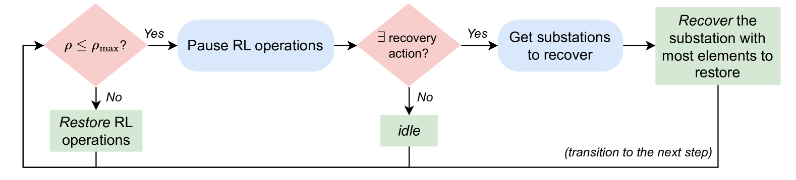
Figure 4: Recovery heuristic based on previous L2RPN solutions and operators’ expertise. When a line surpasses the capacity threshold, the RL agent picks actions to address the risky situations. Otherwise, the heuristic computes the recovery actions to revert the grid topology to its original one. We operate on a maximum of one substation per each step as in real operations.

Given the complexity of topological operations, we introduce two heuristics to assist RL agents. These heuristics incorporate operators’ expert actions—topology recovery and idle actions—into the RL training loop, enhancing performance and sample efficiency in complex, high-dimensional grids. While heuristic-guided approaches have been employed by L2RPN competitors (Donnot,, 2020; Marot et al., 2020a, ), no widely adopted solution currently exists that: (i) is easily accessible to RL practitioners, as most solutions are embedded within L2RPN submissions and design choices; and (ii) has been systematically benchmarked across increasingly complex grids to establish a standard for comparison. RL2Grid’s heuristics fill these gaps by integrating operators’ expertise with best practices from L2RPN solutions (e.g., effective recovery actions). This not only offers a strong baseline for comparison with prior work (Marot et al., 2020a, ; Marot et al.,, 2021), but also incorporates valuable insights from human operators, ensuring practical relevance and improved training efficiency.

The first “idle” heuristic (I) does not perform any operation when line capacities $\rho$ are below the safety threshold of $\rho_{\text{max}}=95\%$. The second heuristic is for topology “recovery” (R) (Figure 4), as it restores the grid’s original topology or performs idle actions when line capacities are below the safety threshold. In more detail, when line capacities exceed the safety threshold, the RL agent selects and executes an action based on the current state to bring the grid back to normal operation. When the grid operates normally (i.e., all line flows are under the safety threshold), the recovery policy takes over. If the grid is in its original topology, the heuristic performs an idle action to proceed with the simulation without changes. Otherwise, the heuristic calculates the actions needed to revert each substation to its original configuration. Considering realistic operational limits (i.e., change at most one substation per step), the heuristic first recovers the substation that is most different from its original configuration. Importantly, the recovery actions do not disrupt RL agent training; instead, they emulate typical human operator behavior. Under normal conditions, system operators prefer to maintain the starting topology. However, it is challenging for an RL agent to learn to restore the original topology in high-dimensional action spaces. For this reason, we anticipate that RL baselines augmented with the recovery policy will drastically improve performance and sample efficiency.

3.2 Safe Operations via Constraints

Modeling safe grid operations through constraints is essential, yet prior approaches such as those developed for the L2RPN challenge have not explored CMDP-based tasks for topology control (Marot et al., 2020a, ; Marot et al.,, 2021; Marot et al., 2022b, ; Chen et al.,, 2022; Kelly et al.,, 2020; Chauhan et al.,, 2023; Zhang et al.,, 2020). RL2Grid bridges this gap by introducing CMDP-based environments that reflect critical operational constraints faced by power system operators, ensuring RL agents are trained under realistic, safety-critical conditions. We define two sets of constraints, based on major primary failure modes that can occur in grid operations:

• Load shedding and islanding constraint (LSI): Failures to meet demand or the creation of electrical islands are treated as a constraint violation, returning a positive cost—this encourages agents to maintain supply-demand balance and ensure grid connectivity consistently. While these are instantaneous constraints in real-world operations, we model them as cumulative constraints (with a zero threshold) to accommodate popular safe RL methods (Su et al.,, 2024; Liu et al., 2021a, ).

  In more detail, let $P_{D,t}$ denote the total demand at time $t$, and $P_{G,t}$ the total generated power. We define the load shedding indicator at $t$ as $L_{t}=\mathbb{1}(P_{G,t}<P_{D,t})$, where $\mathbb{1}(\cdot)$ is the indicator function, which is 1 if the condition inside holds and 0 otherwise. Let $N_{I,t}$ be the number of electrical islands detected in the grid at time $t$ (excluding the main connected component). Define the islanding indicator as $I_{t}=\mathbb{1}(N_{I,t}>0)$. The cost function for LSI at time $t$ is $C_{\text{LSI}}(t)=L_{t}+I_{t}$. Since an episode terminates upon not satisfying the total demand or when an electrical island is detected, we model this instantaneous constraint by setting the constraint threshold to 0 (Stooke et al.,, 2020; Liu et al., 2021b, ; Liu et al., 2021a, ; Su et al.,, 2024; Gu et al.,, 2024). Hence, the policy is considered safe if $C_{\text{LSI}}=0$, meaning no violations occur.

• Transmission line overload constraint (TLO): Overloading lines risks equipment damage and premature failures. It is therefore important to limit the extent to which overloads occur, which is modeled naturally as a cumulative constraint with a specified threshold. Costs are triggered and accumulate each time a line is overloaded, incentivizing agents to manage power flows effectively and avoid prolonged overloads. Specifically, let $P_{F,\ell,t}$ be the power flow on transmission line $\ell$ at time $t$, and let $P_{F,\ell}^{\max}$ be the thermal limit of line $\ell$. Define the overload indicator for line $\ell$ as $O_{\ell,t}=\mathbb{1}(P_{F,\ell,t}>P_{F,\ell}^{\max})$. If a line is overloaded for more than a certain number of time steps (in our environments, 2 time steps), then that line is disconnected by the environment in order to avoid further damage. Let $D_{\ell,t}=\mathbb{1}(\ell\text{ is disconnected})$ be an indicator function for whether line $\ell$ is disconnected by the environment to avoid damage (this does not include disconnections for scheduled maintenance or that are initiated by the opponent). The total overload cost at time $t$ across all transmission lines $\mathcal{L}$ is then $C_{\text{TLO}}(t)=\sum_{\ell\in\mathcal{L}}(O_{\ell,t}+D_{\ell,t})$. The cumulative constraint formulation over an episode is $\sum_{t=0}^{T}C_{\text{TLO}}(t)<\tau$, where $\tau$ is the (hard-coded) constrained threshold.

These constraints are primarily considered across the 32 topological environments, resulting in additional 64 constrained tasks. By formalizing these operational constraints, RL2Grid aims to foster research on RL methods that balance operational effectiveness with strict safety requirements, establishing, to our knowledge, the first benchmark for safe RL in power grid operations.

4 Experiments

We assess the performance of popular RL methods that usually serve as building blocks for more complex algorithms in representative tasks of RL2Grid. In particular, we test: (i) DQN (Mnih et al.,, 2013), PPO (Schulman et al.,, 2017), and SAC (Haarnoja et al.,, 2018) (and their heuristic-integrated versions) on the discrete topological action space for the bus14, bus36-MO-v0, bus118-M, bus118-MOB-v0 tasks over all levels of difficulty (i.e., with increasingly bigger action spaces); (ii) PPO, SAC, and TD3 (Fujimoto et al.,, 2018) in the continuous redispatching action space of these environments; (iii) LagrPPO (Stooke et al.,, 2020) in the two constrained versions (LSI and TLO, described in the previous section) of the discrete topological space for the bus14 task. Our experiments address the following key questions: (i) Can commonly-used model-free RL methods deal with high-dimensional power network operations? (ii) What is the impact of integrating existing task-level knowledge as a heuristic-guided policy within these real-world tasks? (iii) How difficult is it to consider constraints when training an RL agent for power grid operations?

Implementation Details. Data collection is performed on Xeon E5-2650 CPU nodes with 64GB of RAM, using CleanRL-based implementations for the baselines (Huang et al.,, 2022). Complete hyperparameters are in Suppl. F. Additionally, we set a strict time limit on the nodes used for data collection, set to 48 hours. As such, different algorithms have different computational requirements, and some of the baselines run for more steps than others. For example, the heuristic-guided methods are more computationally demanding than the baselines given that they often have to check and compute the reversion actions for the power network, and thus run for considerably fewer steps than the baselines. Given the computational resources used, Suppl. E addresses the associated environmental impact of our experiments and our efforts to offset estimated CO₂ emissions.

Results.

Table 2: Average survival rate (higher is better) for vanilla RL algorithms (V) and their heuristic versions (I for the idle heuristic, R for the heuristic that restores the grid to its original topology) in representative environments (difficulty 0) with topological actions for DQN, PPO, SAC.

		DQN			PPO			SAC
Env.	Diff.	V	I	R	V	I	R	V	I	R
bus14	0	0.07	0.86	0.74	0.74	0.99	0.97	0.17	0.56	0.16
bus36-MO-v0	0	0.04	0.14	0.19	0.06	0.17	0.29	0.01	0.10	0.13
bus118-M	0	0.06	0.17	0.18	0.07	0.13	0.18	0.15	0.18	0.19
bus118-MOB-v0	0	0.07	0.19	0.27	0.04	0.18	0.28	0.01	0.15	0.19

Table 3: Average survival rate (higher is better) of the grid obtained by vanilla RL algorithms (V) in representative environments with continuous redispatching actions for PPO, SAC, TD3.

		PPO	SAC	TD3
Env.	Diff.	V	V	V
bus14	0	0.17	0.01	0.06
bus36-MO-v0	0	0.08	0.02	0.01
bus118-M	0	0.18	0.01	0.01
bus118-MOB-v0	0	0.25	0.08	0.07

Due to the high number of tasks in RL2Grid, we report representative results on the bus14 grid at difficulty 0, referring to Suppl. G for the complete results and training curves of the other levels. In particular, the figures show the average survival smoothed over the last 500 episodes of 5 runs per method, with shaded regions representing the standard error; tables show the average survival at convergence (as described above, survival rate denotes the normalized number of time steps the grid remains operational over an episode, with a survival rate of 1 indicating one month of successful grid operations). Table 2 shows the preliminary results of our topological action spaces evaluation. We indicate with V the original (“vanilla”) model-free baseline, and with I and R the baseline augmented with the heuristics described in Section 3.1 (idle and reconnect, respectively). For these topological cases, we report the results for the first level of difficulty (i.e., level 0, considering 50 discrete actions), and Table 3 shows the results for the redispatching action spaces. Overall, we notice these popular RL baselines struggle to deal with the complexities of power network operations described in Section 2. Considering the lower number of training steps, we also notice that the heuristic-guided versions of the baselines typically achieve higher performance, despite being not nearly sufficient to operate the grid for long periods of time in complex grids.

Figure 5 compares the training performance for model-free baselines, their heuristic-enhanced versions, and constrained variants in the representative bus14 task, which involves topological actions at difficulty level 0. Without the aid of constraints and heuristics, PPO is the only algorithm that successfully learns a good policy for this relatively small grid. However, incorporating human-informed heuristic operations significantly improves performance and sample efficiency across all algorithms. With heuristic augmentation, PPO is able to operate the grid successfully over extended periods, while DQN and SAC also demonstrate strong overall performance. Interestingly, our results suggest that performing idle operations instead of reverting the grid to its original topology increases performance for RL algorithms. On the other hand, enforcing instantaneous or cumulative constraints makes the task considerably more difficult, as agents are penalized for any violations. As a result, LagrPPO struggles even on the bus14 system, failing to achieve effective control while still frequently exceeding the imposed constraint thresholds (more details in Suppl. G).

These results motivate the need for further advancements in RL algorithms that can contend with the complex dynamics and aleatoric uncertainty, long-horizon goals, and hard physical constraints represented within these tasks. By providing common ground for the community, we hope to foster further research on these fronts.

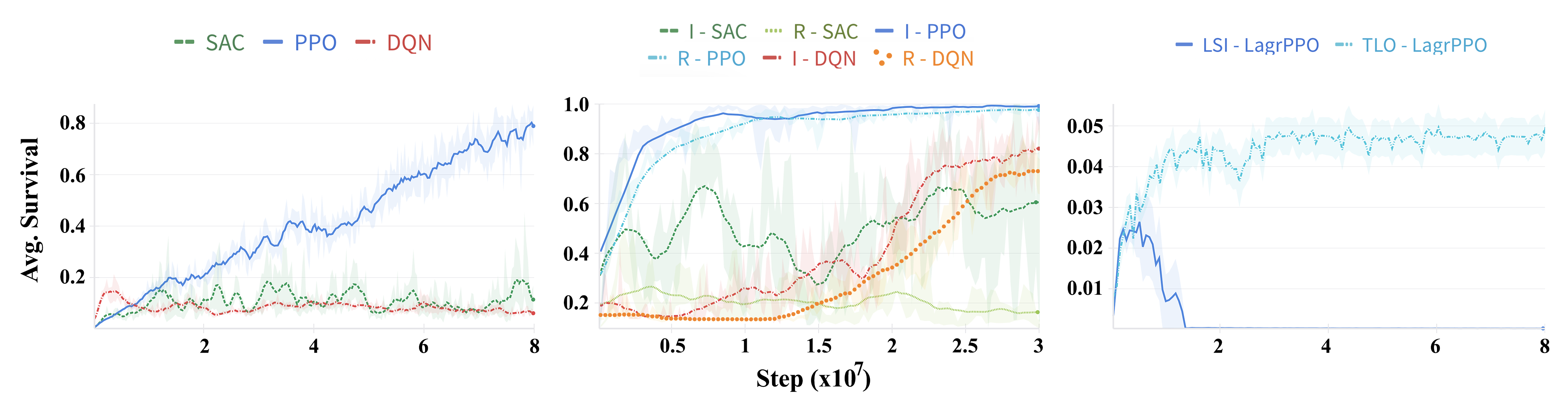
Figure 5: Average survival comparison of model-free RL baselines (left), heuristic-augmented versions (center), and constrained variants (right) on the bus14 task with topological actions at difficulty level 0 (higher values are better). Incorporating heuristics significantly enhances performance and sample efficiency. In contrast, enforcing operational constraints introduces additional challenges, leading to poor performance while failing to satisfy the imposed safety thresholds.

Performance analysis. Figure 6 analyzes how the agent is learning to control the grid. In particular, for each setup considered in the previous section (represented in each row), we show the following three operational components—for clarity, these are visualized as additional reward signals:

• Margin (first column): Represents the cumulative available margin across all transmission lines, where disconnections are penalized and lower power usage is rewarded. Higher values indicate that the agent maintains greater flexibility to handle contingencies. Overall, we find that successful agents tend to maximize line margins.

• Overloads (second column): Measures a cumulative penalty based on the severity and duration of transmission line overloads. Lower values imply that the agent maintains power flows within safe operational limits, which is a key characteristic of effective policies. Unsurprisingly, the unconstrained agents violate the overload constraints. Perhaps surprisingly, the constrained versions actually exhibit even more severe violations of these constraints, which we hypothesize is due to their overall difficulty in optimizing performance in the constrained environment.

• Topology (third column): Quantifies deviations from the initial grid configuration (where all elements are connected to the first bus). A lower value suggests minimal changes, while higher values indicate significant topological modifications. We find that successful agents tend to actively reconfigure the grid to optimize operations.

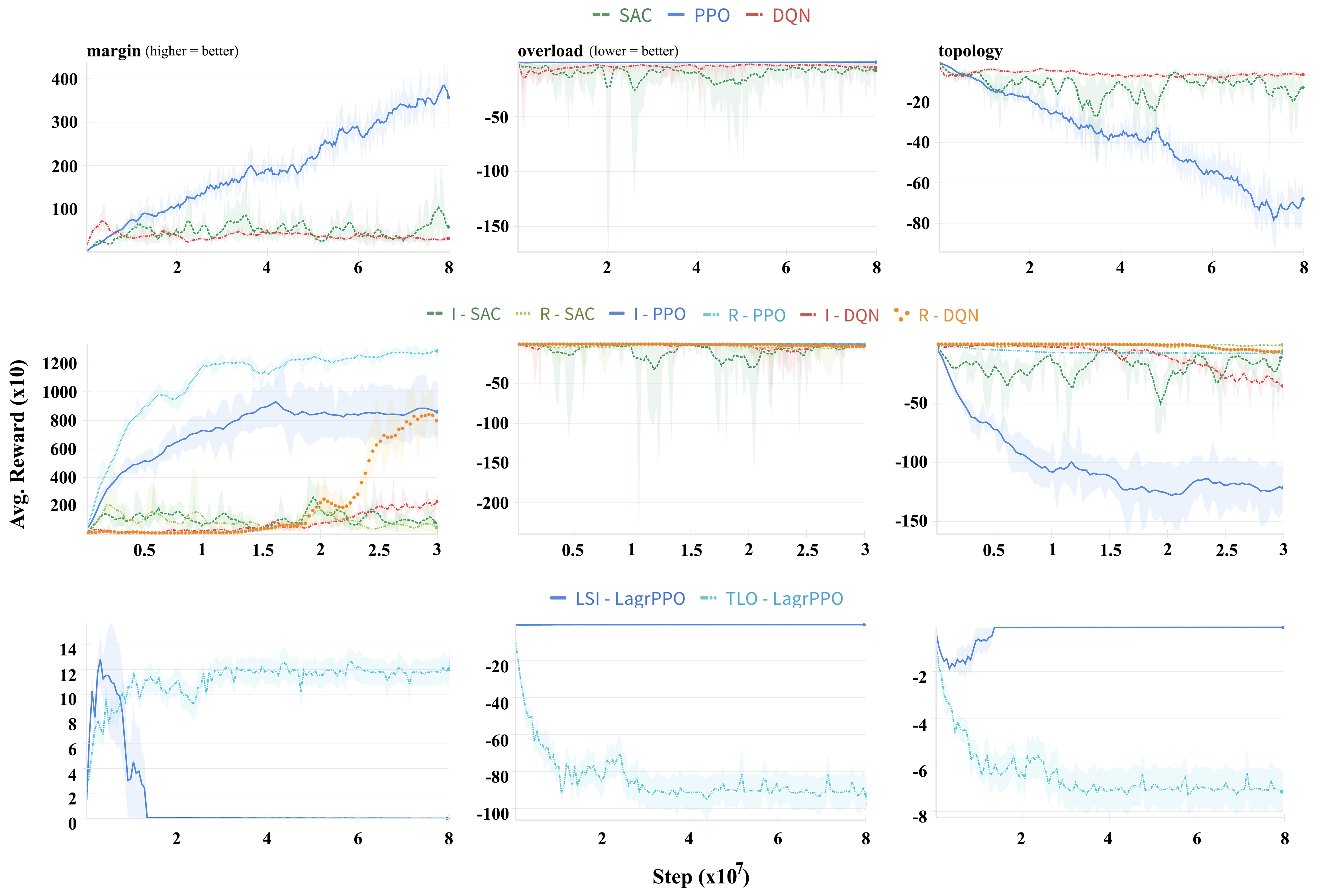
Figure 6: Average (non normalized) reward for key operational components across model-free, heuristic-based, and constrained setups (rows) during training. The first column represents line margins, where higher values indicate better contingency management. The second column tracks overload penalties, with lower values reflecting improved grid stability. The third column captures topology modifications, showing the extent to which agents reconfigure the grid.

5 Related Work

There have been several attempts to develop benchmarks for sequential decision-making in power system operations, but they often focus on smaller-scale problems and/or simplified setups (Chen et al.,, 2022). Examples include python-microgrid for simulating microgrids (Henri et al.,, 2020), CityLearn for demand response and urban energy management (Vazquez-Canteli et al.,, 2020), and gym-ANM for small electricity distribution networks (Henry and Ernst,, 2021). RL environments for electric vehicle (EV) charging and electricity markets have also been introduced (Zhang et al.,, 2020). Recently, SustainGym spanned diverse tasks ranging from EV charging to carbon-aware data center job scheduling (Yeh et al.,, 2023). The ARPA-E GO Competition provides a realistic, large-scale benchmark for power grid operations (ARPA-E,, 2023), but is more-so geared towards offline optimization approaches than online sequential decision-making. On the methodological side, recent contributions in the field include works on cascading failure mitigation, demand response optimization, and real-time grid control using RL (Matavalam et al.,, 2022; Lehna et al.,, 2023; van der Sar et al.,, 2024). Nonetheless, these works are more geared towards methodological advancements rather than proposing a benchmark. For this reason, we refer the reader to recent reviews for details on RL applications in power grid operations (Li et al.,, 2023; Su et al.,, 2024).

6 Tackling the Challenges of Power Grids with RL

Applying RL in power grids presents numerous open problems, each offering significant opportunities for advancing both grid operations and RL methodologies (Marot et al., 2022b, ). While we address a subset of these challenges via our benchmark, there remains ample room for future work.

6.1 RL Methodologies of Importance for Power Grids

Different RL techniques have the potential to be beneficial in addressing open grid problems. However, there are also potential risks—e.g., with respect to safety, reliability, and robustness—that are important to address. In the following, we summarize interesting avenues for future research.

Safe RL. Safety is paramount in grid operations. Safe RL methods aim to ensure that learning and control policies adhere to strict safety constraints, preventing actions that could lead to blackouts or equipment damage (Donnot,, 2020). Ensuring safety while optimizing performance is a critical area of research (Garcıa and Fernández,, 2015; Marzari et al.,, 2025). In particular, incorporating novel CMDP-based algorithms and formal methods can be particularly beneficial for ensuring that solutions adhere to physical and operational limits (Liu et al., 2021b, ; Marchesini et al.,, 2023).

Human-in-the-loop. Effective grid management requires human expertise and intervention. Incorporating human supervision, interaction, and feedback into RL systems allows for a synergistic approach where human operators and AI work together to optimize grid operations (Marot et al., 2022b, ). This collaboration can enhance decision-making and build trust in AI-driven solutions.

Hierarchical control and multi-agent RL. Power grids operate across many hierarchical levels, from individual substations to entire regions. Effective coordination within and across these levels is crucial for maintaining efficient and reliable operations. Hierarchical RL methods can be developed to manage multi-level control tasks, in a way that addresses the scale and complexity of grid operations (Pateria et al.,, 2021; Aydeniz et al.,, 2023). Another promising direction is the use of multi-agent representations. Given the vast and distributed nature of power grids, scalability can be enhanced by dividing the grid into distinct agents, each responsible for its own operations. Multi-agent RL (MARL) frameworks can enable these agents to learn and coordinate actions (Papoudakis et al.,, 2021; Marchesini et al.,, 2024), to improve overall grid performance while managing local contingencies more effectively.

Robust RL. The integration of renewable energy sources introduces significant variability and uncertainty into power grids, leading to non-stationary environments. RL algorithms need to adapt to these evolving dynamics to ensure stable and efficient grid operations despite fluctuating supply and demand profiles. Handling non-stationarity and generalization are thus critical research directions (Moos et al.,, 2022; Marchesini and Amato,, 2023).

Model-based RL. Model-based RL methods leverage models of the grid dynamics to improve learning efficiency and policy performance. These methods can provide more accurate predictions and better generalize across different scenarios, leading to faster and more robust solutions (Luo et al.,, 2022). Additionally, the AlphaZero algorithm, which combines tree search with deep learning, has shown remarkable success in games like chess and Go and could offer new strategies for handling complex, sequential decision-making tasks with high-dimensional spaces (Liu et al.,, 2023).

Better representations. Improving model representations for RL in power grids can also lead to more efficient learning and better policy performance. Leveraging graph neural networks (GNNs) offers a potential avenue for advancement. Power grids can be naturally represented as graphs, with nodes representing buses and edges representing transmission lines. GNNs can effectively model these structures, capturing the spatial and topological dependencies inherent in power grids. Integrating GNNs with RL algorithms can enhance the representation and learning of grid dynamics.

Non-RL approaches. While RL holds great promise, it is also essential to consider non-RL approaches such as optimization solvers, which are relevant particularly for problems with well-defined optimization objectives and constraints. In addition, exploring hybrid methods that combine RL with traditional optimization techniques can yield powerful tools for complex grid management tasks.

6.2 Improving Realism of Power Grid Environments

While RL2Grid aims to promote initial advancements in RL methodologies of relevance to power grids, it is important to acknowledge that this is only a first step. Notably, building on these advancements to develop “last-mile” deployed solutions will require further improvements in the realism of power grid environments. We highlight several important directions in this regard.

Scalability. Realistic power systems akin to those managed by RTE France and other transmission system operators may capture hundreds to thousands of buses. To ensure that RL solutions are applicable to real-world scenarios, improving the size and scale of grid environments is essential.

Real data. Grid2Op (and thus, RL2Grid) relies on realistic but synthetic data, which already provide significant challenges for RL. After scaling up RL to deal with the challenges provided by RL2Grid, future environments should (in a way that is cognizant of privacy issues) publicly release real or more realistic synthetic grid data to design to bridge the gap with real power grid operations.

N-1 security. Grid operators must ensure the system can withstand failure of any single component. Rather than modeling failures via random opponents, environments should handle this exhaustively and/or through adversarial agents tailored specifically to the method being tested.

Topology vs. redispatch. Different grid operators handle the relationship between redispatch and topology optimization differently (e.g., some co-optimize these processes, whereas others prefer to handle them separately). Future benchmarks should reflect this heterogeneity in how different power grids are managed. Moreover, Grid2Op’s current approach of disconnecting lines after unaddressed overloads does not fully capture real-world practices, where operators attempt to prevent overheating at all costs. Incorporating more realistic consequences for unaddressed overloads, such as system costs, can improve the fidelity of benchmarks. Additionally, grid operators cannot switch every element to every busbar, and there are limits on the number of connected components per substation. Reflecting these constraints can lead to more practical and applicable RL solutions. Storage assets also play an increasingly important role in grid operations. Future benchmarks should accurately model storage and clarify the extent of control grid operators have over these assets.

Phase-shift transformers. Phase-shift transformers, currently modeled as integer variables in the action space, should be represented more accurately to reflect their operational impact. Maintenance activities also vary significantly, with Type A involving physical presence at the site and Type B allowing remote interventions. Differentiating these types of maintenance activities in benchmarks can provide a more accurate representation of real-world constraints.

7 Conclusions

Power grids are essential in combating climate change, requiring a transition to low-carbon energy and enhanced resilience against climate-induced extremes. The integration of variable renewable energy sources introduces complexities and uncertainties in grid operations, posing significant challenges for human operators and traditional power system solvers. Our work aims to foster progress towards these challenges by introducing RL2Grid, a benchmark designed to bridge the gap between current grid management practices and methodological research in RL. RL2Grid provides a standardized interface for power grid environments, featuring common rewards, state spaces, action spaces, and safety constraints across a pre-designed set of diverse and complex grid tasks in order to provide a common ground for monitoring and promoting progress. We perform a comprehensive evaluation of the performance of DQN, PPO, LagrPPO, SAC, and TD3 on RL2Grid tasks, including versions augmented with domain-informed heuristics aimed at improving performance and sample efficiency, and find that there is still significant room for improvement in the performance of these methods. By offering a standardized platform for RL research in the context of power grids, RL2Grid aims to accelerate algorithmic innovation towards improving power grid operations amidst the evolving challenges posed by climate change.

Appendix A Relationship of RL2Grid to L2RPN tasks and solutions

In this section, we clarify the relationship of the tasks presented within RL2Grid, as well as the baseline methods evaluated, to the tasks and solutions presented within the L2RPN competition series.

Tasks. RL2Grid employs all the main Grid2Op “base environments” (which are likewise employed in L2RPN). However, the solutions developed for L2RPN relied on different customized components. Every competition relied on different time series, making effective comparisons far from trivial. For these reasons, on top of the standardization proposed in our work (see Section 3), we have made some underlying changes to the base environments to better reflect the current and future challenges of RL research. Examples include (i) episodes with longer horizons (i.e., an RL2Grid episode models a month of grid operations, $\sim$8000 steps, compared to weekly episodes of most prior work); (ii) making the tasks as uniform as possible (i.e., by integrating curtailment operations in all Grid2Op tasks); (iii) enabling simulation steps inside the Gymnasium interface (a feature added in our code revision, which is not currently available in Grid2Op). These decisions were driven by our goal of ensuring that our benchmark is accessible, standardized, and provides a clear starting point for researchers who may not be familiar with the nuances of these competitions and power grids.

Baselines. Due to the different choices of input features and action spaces considered by different methods submitted to the L2RPN challenges, it was not possible to directly benchmark these specific methods on the RL2Grid tasks. However, the baselines chosen are representative of the methods submitted to past L2RPN competitions, in addition to representing commonly-used methods within the RL community as a whole. In particular, within the L2RPN submissions, a common approach was to incorporate heuristics. These heuristics varied significantly between methods and pushed us to design one that mimicked human operations in real grid operations. We developed this heuristic in collaboration with power system operators who have contributed to our work, incorporating fundamental insights from previous solutions while keeping the focus on standardization and benchmarking.

Appendix B RL baselines

In this section, we briefly introduce the baseline RL algorithms employed in our evaluation, referring to the original papers for exhaustive details about these methods (Mnih et al.,, 2013; Schulman et al.,, 2017; Haarnoja et al.,, 2018; Fujimoto et al.,, 2018).

DQN (Mnih et al.,, 2013). A DQN agent uses a neural network to approximate the action value function $Q$ by taking as input the state of the environment and outputting $Q$-values for every possible action. During training, the agent uses an $\epsilon$-greedy policy to select random actions or follow the greedy policy on these $Q$-values, according to a linearly decaying probability $\epsilon$. The $Q$ network is thus updated to minimize the difference between predicted $Q$-values and a target derived from actual rewards and future $Q$-values. To deal with overestimation, we use Double-DQN (van Hasselt et al.,, 2016) and decouple action selection from action evaluation using a target $Q$ network. Due to its value-based nature, a DQN agent can only consider discrete (topological) actions.

PPO (Schulman et al.,, 2017) and Lagrangian PPO (LagrPPO) (Stooke et al.,, 2020). A PPO agent uses its neural network to directly approximate a policy. The agent learns the policy parameters by simplifying the TRPO (Schulman et al.,, 2015) algorithm, using a computationally tractable clipped objective. This clipping mechanism prevents large changes to the policy that could destabilize the training. At a high level, such a surrogate objective balances policy improvement and limits the divergence between policy updates. To drive the policy training, PPO also learns an advantage function to determine how much better (or worse) taking an action is compared to the expected value. By employing different probability distributions as a policy, a PPO agent can deal with both continuous (redispatching) and discrete (topological) actions. The Lagrangian version applies the same intuitions while learning additional value functions for each constraint. It then changes to policy training by considering the Lagrangian in Equation 2. In more detail, Lagrangian algorithms take gradient ascent steps in $\pi$ and descent steps in $\bm{\lambda}$ to trade off safety and task performance. These methods focus on satisfying the constraints using penalties $\bm{\lambda}$ that grows unbounded when constraints are violated. When constraints are satisfied, $\bm{\lambda}$ scale down (to zero), allowing the algorithm to maximize the task objective.

SAC (Haarnoja et al.,, 2018). Similarly to PPO, a SAC agent learns different networks to maintain a policy and two value functions that mitigate positive bias in value estimates. Overall, the agent maximizes both the expected return and the entropy of the policy. The entropy term encourages exploration by promoting stochastic policies, which helps prevent premature convergence to suboptimal policies. In terms of actions, the SAC agent can deal with the same action types as PPO.

TD3 (Fujimoto et al.,, 2018). A TD3 agent learns multiple networks similarly to SAC. However, unlike the stochastic policies learned by PPO and SAC, TD3 learns a deterministic policy and can only deal with continuous actions. To encourage exploration, the agent does not maximize the entropy of the policy but adds noise to the output of the policy network.

Appendix C Environments

Table C.1: Action space sizes for the considered environments. Left: Difficulty for environments with a (discrete) topology-based action space. Right: (continuous) redispatching and curtailment tasks.

	# Actions per difficulty level
	Topology (T)					Redispatching and curtailment (R)
	0	1	2	3	4	0
bus14	50	209	-	-	-	6
bus36-M	50	302	1829	11071	66978	22
bus36-MO-v0	50	302	1829	11071	66978	22
bus36-MO-v1	50	302	1829	11071	66978	22
bus118-M	50	308	1903	11744	72461	69
bus118-MOB-v0	50	309	1914	11849	73328	69
bus118-MOB-v1	50	309	1915	11852	73357	69

As discussed in Section 3, here we introduce the different levels of difficulty for the topological-based environments, as well as the reward function employed in all the tasks. Each increasing level of task difficulty corresponds to a higher dimensional discrete action space. Table C.1 summarizes the difficulty levels and the corresponding total number of actions.

C.1 Action Spaces Analysis

In this section, we visually analyze the action spaces of one representative environment for each power grid size (i.e., bus14, bus36-MO-v0, bus118-M).

For each difficulty level, Figures C.1, LABEL:, C.2, LABEL: and C.3 show the percentage of actions considered for each substation within the action space. The x-axis lists the substation IDs in descending order based on the number of available actions. The y-axis represents the ratio of actions used in the action space to the total number of available actions for each substation. Consequently, the highest difficulty level indicates that the action space includes all possible actions for all substations. Overall, this analysis suggests that the substation with the most electric components (i.e., the most possible topologies) is best suited to handle contingencies.

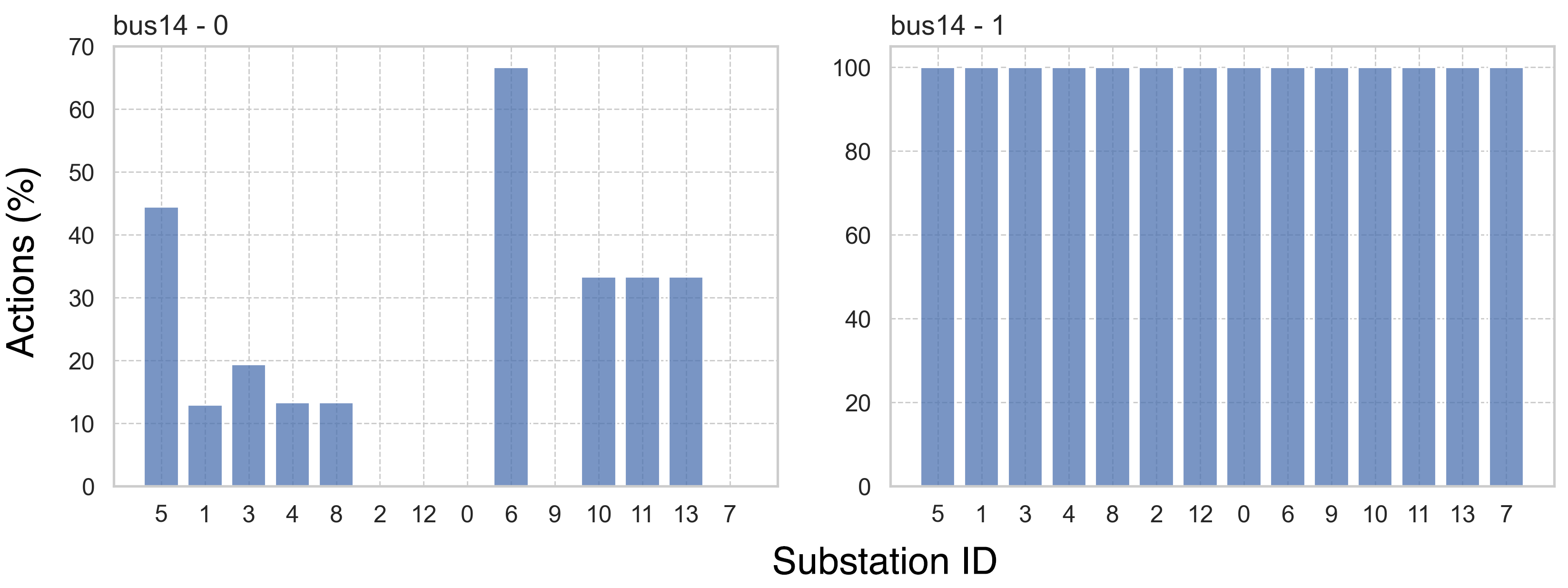
Figure C.1: Percentage of actions considered for each substation within the action space for bus14 (discrete) topological tasks (difficulty level is indicated with the number on the top left).

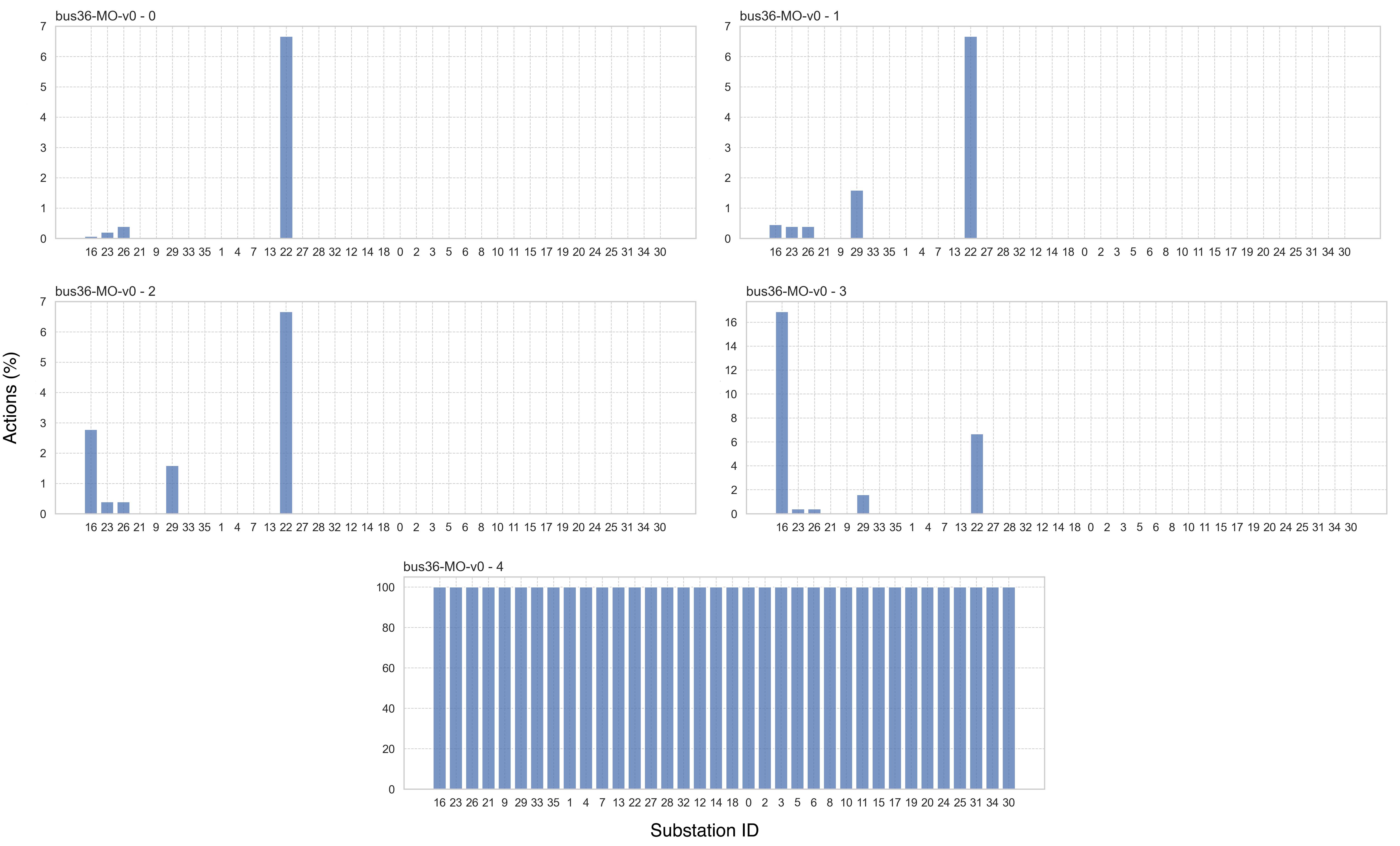
Figure C.2: Percentage of actions considered for each substation within the action space for bus36-MO-v0 (discrete) topological tasks (difficulty level is indicated with the number on the top left).

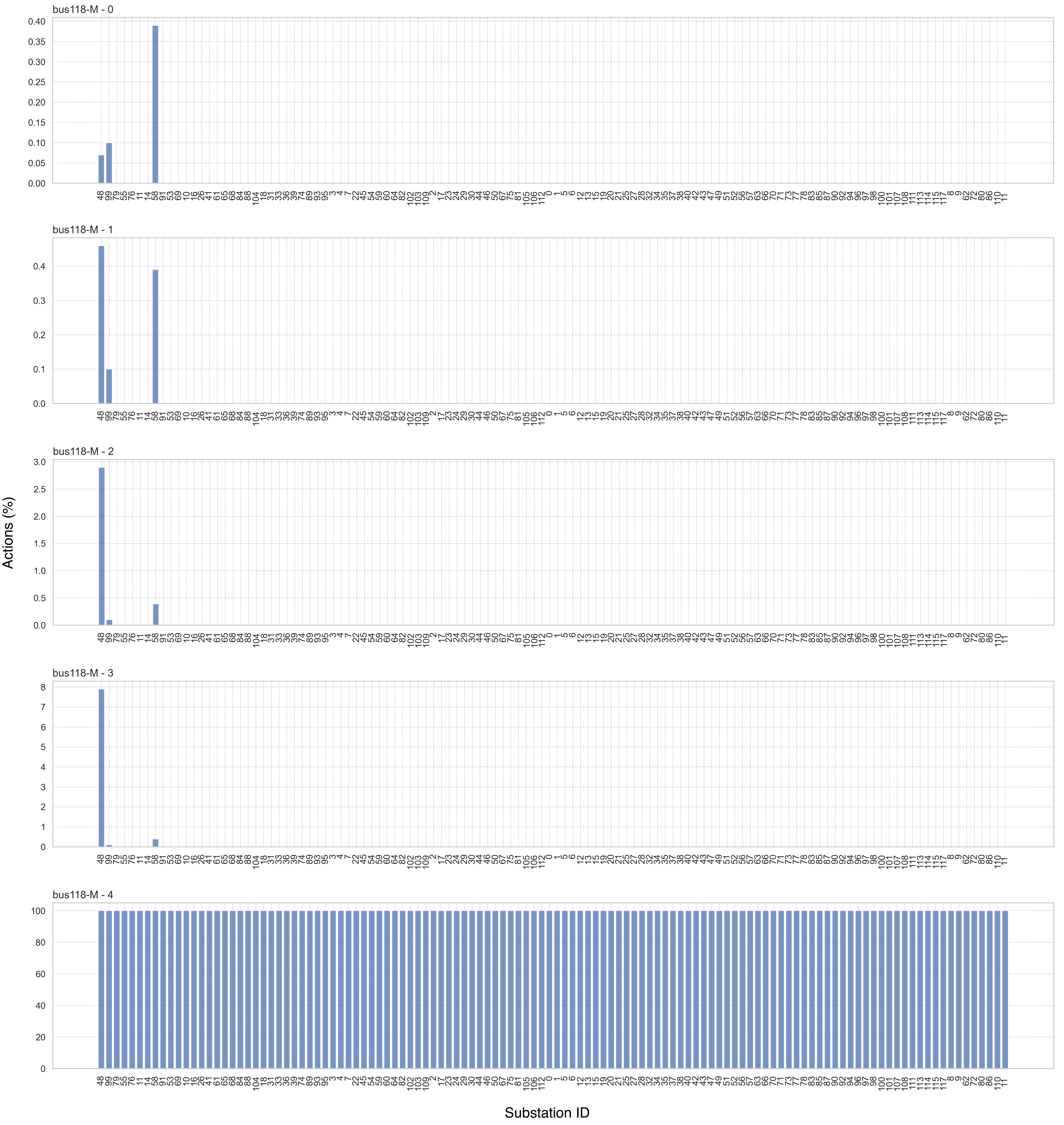
Figure C.3: Percentage of actions considered for each substation within the action space for bus118-M (discrete) topological tasks (difficulty level is indicated with the number on the top left).

Figures C.4, LABEL: and C.5 then present the data collected during the action ranking mechanism described in Section 3.

As a sanity check, Figure C.4 shows an example of the uniform sampling strategy used to select which action to simulate at each simulation step. The x-axis shows the total number of actions for the bus14 (discrete) topological task; the y-axis indicates the number of times each action was sampled during the ranking process.

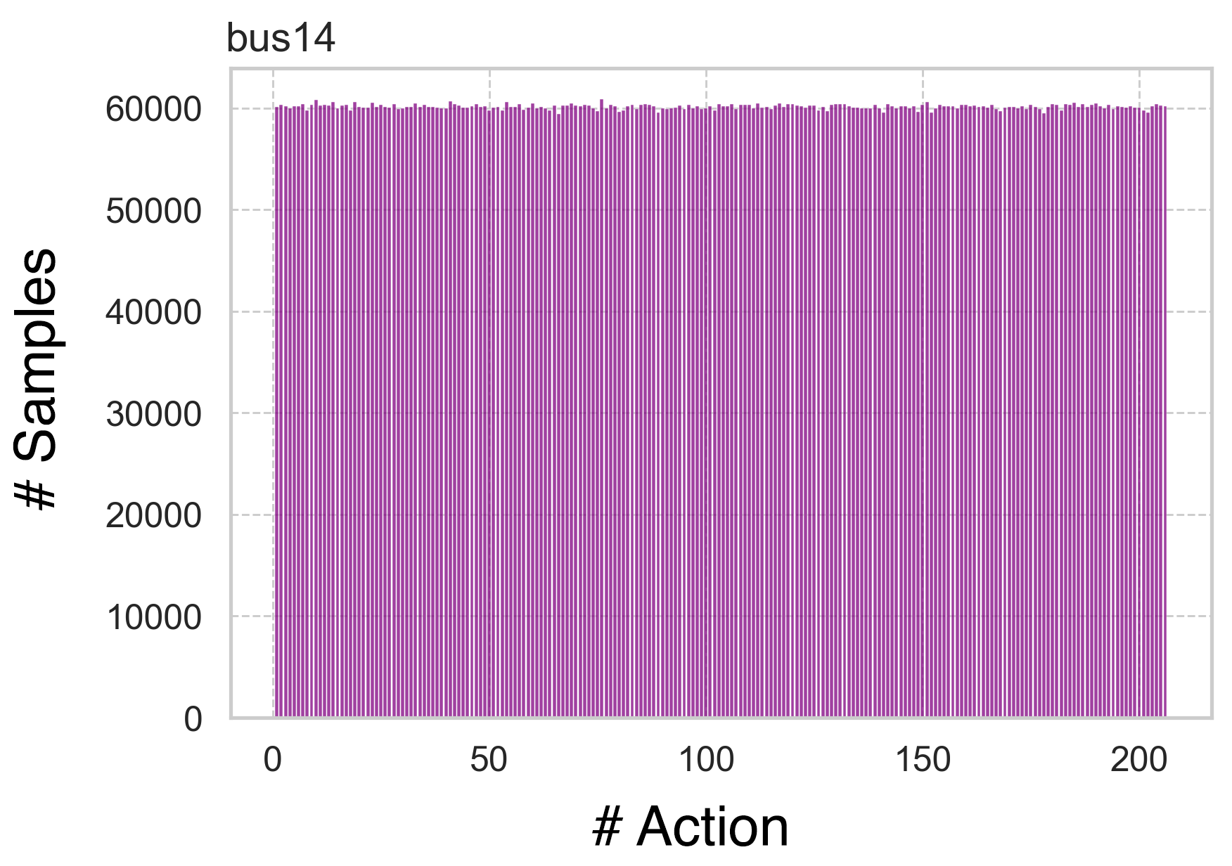
Figure C.4: Number of times each action is sampled over the ranking process time.

Figure C.5 shows the final ranking of the actions for the three representative environments. The x-axis shows the total number of actions for each task; the y-axis indicates the average survival rate of each action during the ranking process. Crucially, most of the actions are relevant (i.e., with a high survival rate) in the tasks, motivating the increasing levels of difficulty we proposed for the (discrete) topological environments.

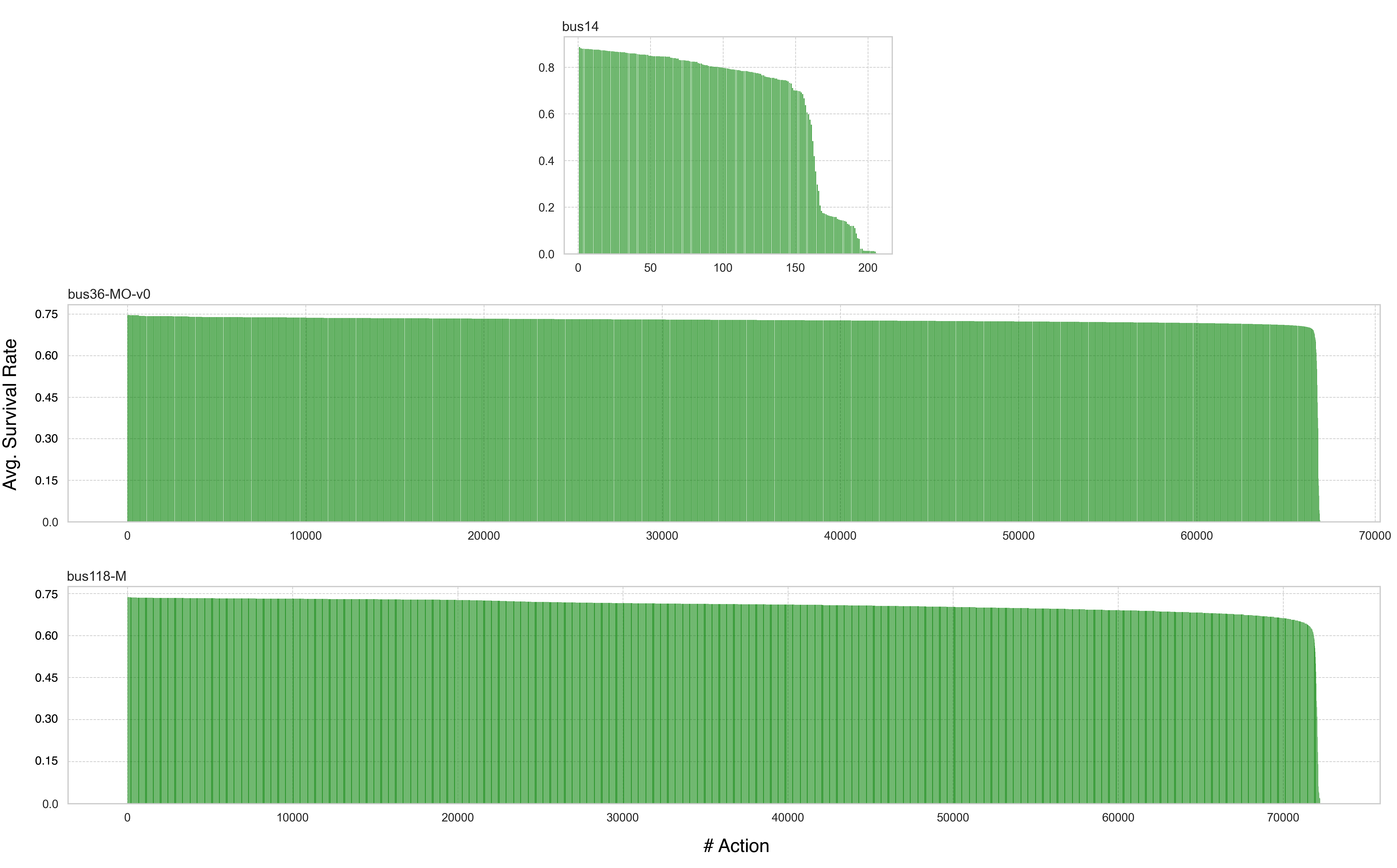
Figure C.5: Average survival rate of the action spaces after the ranking process time.

Appendix D State Space

Regardless of the task, at a certain time-step $t$ an agent gets the following set of features: $[t,\text{Gen}_{P},\text{Gen}_{\theta},\text{Load}_{P},\text{Load}_{\theta},\rho,\text{Cooldown}_{\text{lines}}]$. Additionally, based on the nature of the task, the agent can observe additional features as follows:

• Topological actions: when an agent operates using (discrete) topological actions, it observes $[$Topo_vect, Line_status, Time_overflow, Time_sub-cooldown$]$.

• Redispatching actions: when an agent operates using (continuous) redispatching actions, it observes $[$Tg_dispatch, Curr_dispatch, Gen_margin-up, Gen_margin-down$]$.

• Curtailment actions: when an agent operates using (continuous) curtailment actions, it observes $[$Gen_Pcurt, Curtail, Curtail_limit$]$.

• Maintenance: when the task has maintenance contingencies (see Table 1), the agent gets $[$Time_next-maint, Duration_next-maint$]$.

• Storage: when the task has batteries (see Table 1), the agent gets $[$Storage_charge, Storage_powertg, Storage_power, Storage_$\theta$$]$.

Such a distinction is useful to reduce the size of the space the agent can observe when there are features that are not relevant to a specific task. For example, if an agent uses only discrete actions (topology), then everything related to target dispatch, actual dispatch, and storage is irrelevant as they will not change. Likewise, if an agent uses only continuous actions, it is not necessary to include features related to “topology” as they will not be modified. Additionally, all the features related to voltage (e.g., voltage for generators, loads, $\dots$) and reactive values (e.g., reactive power for generator, loads, $\dots$) can be neglected.

For the interested RL practitioner, we refer to the original Grid2Op documentation for exhaustive descriptions of these features (Donnot,, 2020).

Appendix E Environmental Impact

Despite each training run being “relatively” computationally inexpensive due to the use of CPUs, the experiments of our evaluation led to cumulative environmental impacts due to computations that run on computer clusters for an extended time. Our experiments were conducted using a private infrastructure with a carbon efficiency of $\approx 0.275\frac{\text{kgCO${}_{2}$eq}}{\text{kWh}}$, requiring a cumulative $\approx$720 hours of computation. Total emissions are estimated to be $\approx 20.79\text{kgCO${}_{2}$eq}$ using the Machine Learning Impact calculator, and we purchased offsets for this amount through Treedom. We do not directly estimate or offset other categories of environmental impacts (such as water usage or embodied hardware impacts), though recognizing that these are additionally important to consider.

Appendix F Hyperparameters

Table F.1 lists the hyperparameters considered during our initial grid search and the final (best-performing) parameters used for our experiments.

Table F.1: Details of the grid search used to find the best-performing hyperparameters for each algorithm in the topological (T) and redispatching (R) cases.

Algorithm	Parameter	Grid search	Chosen value (T - R)
Shared	N° parallel envs	10	10
	Learning starts	20000	20000
	Time limit	48 hours	48 hours
	Max gradient norm	10, 20, 50	10
	Discount $\gamma$	0.9, 0.95, 0.99	0.9
	Batch size	64, 128, 256	128
	$\alpha$	0.1, 0.3, 0.6	0.1
	$\beta$	0.1, 0.3, 0.6	0.3
	$\eta$	0.1, 0.3, 0.6	0.3 - 0.6
	$\omega$	0.1, 0.3, 0.6	0.3
	$\lambda$	0, 50	0 (TLO), 50 (LSI)
DQN	Train frequency	20, 100, 1000	20
	Target network update	500, 1000, 10000	1000
	Buffer size	100000, 250000, 500000, 1000000	500000
	Learning rate	0.003, 0.0003, 0.00003	0.0003
	$\epsilon$-decay fraction	0.3, 0.5 0.7	0.5
PPO	N° steps	10000, 20000, 50000	20000
	N° update epochs	20, 40, 80	40
	Actor learning rate	0.003, 0.0003, 0.00003	0.0003 - 0.00003
	Critic learning rate	0.003, 0.0003, 0.00003	0.0003 - 0.00003
	$\epsilon$-clip	0.1, 0.2, 0.3	0.2
SAC	Train frequency	20, 100, 1000	20
	Actor delayed update	2, 4	2
	Noise clip	0.5	0.5
	Buffer size	100000, 250000, 500000, 1000000	500000
	Actor learning rate	0.003, 0.0003, 0.00003	0.0003 - 0.00003
	Critic learning rate	0.003, 0.0003, 0.0003	0.0003 - 0.00003
	Entropy regularization	0.2	0.2
	Noise clip	0.5	0.5
TD3	Actor delayed update	2, 4	2
	Buffer size	100000, 250000, 500000, 1000000	500000
	Actor learning rate	0.003, 0.0003, 0.00003	0.0003 - 0.00003
	Critic learning rate	0.003, 0.0003, 0.00003	0.0003 - 0.00003
	$\tau$	0.005, 0.0005	0.005
	Policy noise	0.2	0.2
	Exploration noise	0.1	0.1

Appendix G Omitted Figures in Section 5

Figure G.1 shows the training curves for the (discrete) topological action spaces. Due to the strict time limit imposed on the computation nodes (see Section 4) and the different computational requirements of the algorithms, not all the baselines perform the same number of steps in the time limit. Additionally, despite the grid search of Table F.1, some baselines achieved lower performance than expected (e.g., SAC and DQN in the bus14 scenarios). We will keep working on the benchmark to find better parameters, run longer experiments, and keep the following Figures updated.

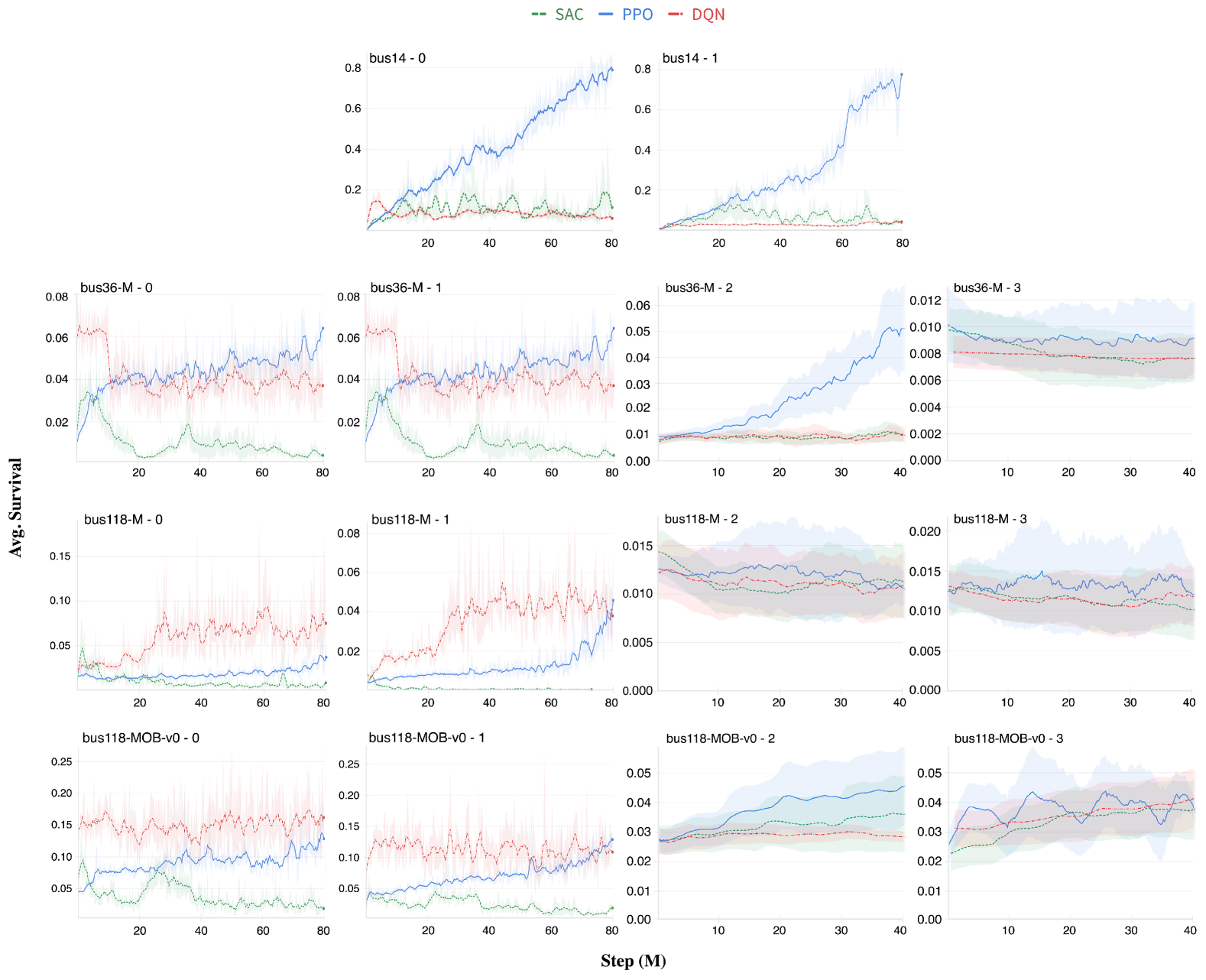
Figure G.1: Average survival rate for the discrete topological case in bus14, bus36-M, bus118-M, bus118-MOB-v0 using the SAC, PPO, and DQN baselines. We indicate the difficulty level (ranging from 0 to 3) next to the environment identifier.

Figure G.2 shows the training curves for the (continuous) redispatching action spaces.

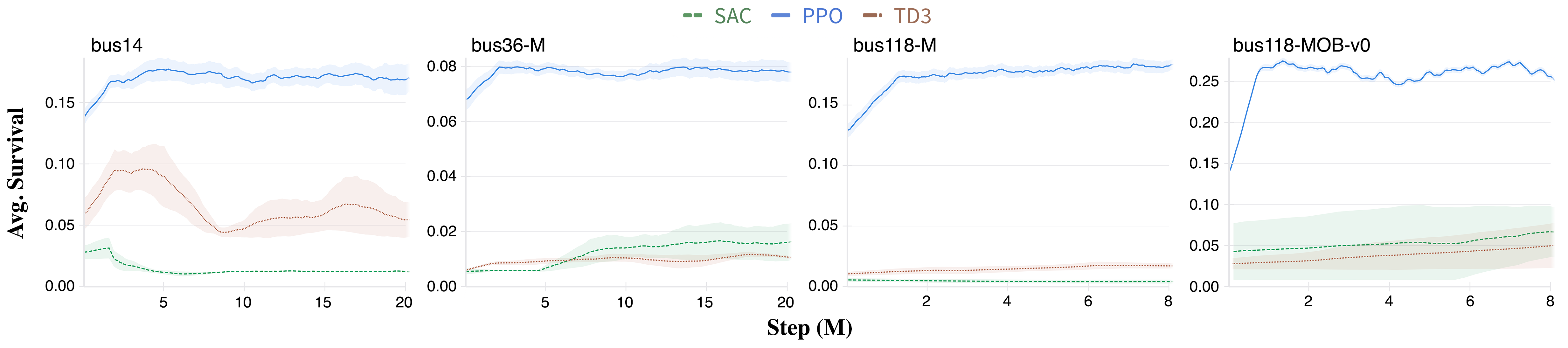
Figure G.2: Average survival rate for the continuous redispatching case in bus14, bus36-M, bus118-M, bus118-MOB-v0 using the SAC, PPO, and TD3 baselines.

Figure G.3 shows the cost obtained over the training for the constrained experiments.

Figure G.3: Average cost rate for constrained case in the representative bus14 using the LagrPPO baseline. The constrained threshold (red line) is set to 0 and 50 for the TLO and LSI cases, respectively.

References

- Altman, (1998) Altman, E. (1998). Constrained markov decision processes with total cost criteria: Lagrangian approach and dual linear program. In Mathematical methods of Operations Research.
- ARPA-E, (2023) ARPA-E (2023). Grid Optimization (GO) Competition. https://gocompetition.energy.gov/.
- Aydeniz et al., (2023) Aydeniz, A. A., Marchesini, E., Loftin, R., and Tumer, K. (2023). Entropy maximization in high dimensional multiagent state spaces. In 2023 International Symposium on Multi-Robot and Multi-Agent Systems (MRS), pages 92–99.
- Chauhan et al., (2023) Chauhan, A., Baranwal, M., and Basumatary, A. (2023). Powrl: A reinforcement learning framework for robust management of power networks. In AAAI.
- Chen et al., (2022) Chen, X., Qu, G., Tang, Y., Low, S., and Li, N. (2022). Reinforcement learning for selective key applications in power systems: Recent advances and future challenges. IEEE Transactions on Smart Grid, 13(4):2935–2958.
- Donnot, (2020) Donnot, B. (2020). Grid2op- A testbed platform to model sequential decision making in power systems. . https://GitHub.com/rte-france/grid2op.
- Fujimoto et al., (2018) Fujimoto, S., van Hoof, H., and Meger, D. (2018). Addressing function approximation error in actor-critic methods. In International Conference on Machine Learning (ICML).
- Garcıa and Fernández, (2015) Garcıa, J. and Fernández, F. (2015). A comprehensive survey on safe reinforcement learning. In Journal of Machine Learning Research (JMLR).
- Gu et al., (2024) Gu, S., Yang, L., Du, Y., Chen, G., Walter, F., Wang, J., and Knoll, A. (2024). A review of safe reinforcement learning: Methods, theories and applications. IEEE Transactions on Pattern Analysis and Machine Intelligence.
- Haarnoja et al., (2018) Haarnoja, T., Zhou, A., Abbeel, P., and Levine, S. (2018). Soft actor-critic: Off-policy maximum entropy deep reinforcement learning with a stochastic actor. In International Conference on Machine Learning (ICML).
- Henri et al., (2020) Henri, G., Tanguy Levent, A. H., Alami, R., and Cordier, P. (2020). pymgrid: An open-source python microgrid simulator for applied artificial intelligence research. arXiv.
- Henry and Ernst, (2021) Henry, R. and Ernst, D. (2021). Gym-anm: Open-source software to leverage reinforcement learning for power system management in research and education. Software Impacts, 9.
- Huang et al., (2022) Huang, S., Dossa, R. F. J., Ye, C., Braga, J., Chakraborty, D., Mehta, K., and Araújo, J. G. (2022). Cleanrl: High-quality single-file implementations of deep reinforcement learning algorithms. Journal of Machine Learning Research, 23(274):1–18.
- Kelly et al., (2020) Kelly, A., O’Sullivan, A., de Mars, P., and Marot, A. (2020). Reinforcement learning for electricity network operation. arXiv.
- Lehna et al., (2023) Lehna, M., Jan Viebahn, C. S., Marot, A., and Tomforde, S. (2023). Managing power grids through topology actions: A comparative study between advanced rule-based and reinforcement learning agents. Energy and AI.
- Li et al., (2023) Li, Y., Yu, C., Shahidehpour, M., Yang, T., Zeng, Z., and Chai, T. (2023). Deep reinforcement learning for smart grid operations: Algorithms, applications, and prospects. Proceedings of the IEEE, 111(9):1055–1096.
- Liu et al., (2023) Liu, S., Liu, J., Ye, W., Yang, N., Zhang, G., Zhong, H., Kang, C., Jiang, Q., Song, X., Di, F., et al. (2023). Real-time scheduling of renewable power systems through planning-based reinforcement learning. arXiv preprint arXiv:2303.05205.
- (18) Liu, Y., Halev, A., and Liu, X. (2021a). Policy learning with constraints in model-free reinforcement learning: A survey. In Proceedings of the Thirtieth International Joint Conference on Artificial Intelligence, IJCAI-21, pages 4508–4515.
- (19) Liu, Y., Halev, A., and Liu, X. (2021b). Policy learning with constraints in model-free reinforcement learning: A survey.
- Luo et al., (2022) Luo, F.-M., Xu, T., Lai, H., Chen, X.-H., Zhang, W., and Yu, Y. (2022). A survey on model-based reinforcement learning.
- Marchesini and Amato, (2023) Marchesini, E. and Amato, C. (2023). Improving deep policy gradients with value function search. In The Eleventh International Conference on Learning Representations.
- Marchesini et al., (2024) Marchesini, E., Baisero, A., Bhati, R., and Amato, C. (2024). On stateful value factorization in multi-agent reinforcement learning.
- Marchesini et al., (2023) Marchesini, E., Marzari, L., Farinelli, A., and Amato, C. (2023). Safe deep reinforcement learning by verifying task-level properties. In International Conference on Autonomous Agents and MultiAgent Systems (AAMAS).
- (24) Marot, A., Donnot, B., Chaouache, K., Kelly, A., Huang, Q., Hossain, R.-R., and Cremer, J. L. (2022a). Learning to run a power network with trust. Electric Power Systems Research, 212:108487.
- Marot et al., (2021) Marot, A., Donnot, B., Dulac-Arnold, G., Kelly, A., O’Sullivan, A., Viebahn, J., Awad, M., Guyon, I., Panciatici, P., and Romero, C. (2021). Learning to run a power network challenge: a retrospective analysis. In NeurIPS 2020 Competition and Demonstration Track, pages 112–132. PMLR.
- (26) Marot, A., Donnot, B., Romero, C., Donon, B., Lerousseau, M., Veyrin-Forrer, L., and Guyon, I. (2020a). Learning to run a power network challenge for training topology controllers. Electric Power Systems Research, 189:106635.
- (27) Marot, A., Kelly, A., Naglic, M., Barbesant, V., Cremer, J., Stefanov, A., and Viebahn, J. (2022b). Perspectives on future power system control centers for energy transition. Journal of Modern Power Systems and Clean Energy, 10(2):328–344.
- (28) Marot, A., Megel, N., Renault, V., and Jothy, M. (2020b). ChroniX2Grid - The Extensive PowerGrid Time-serie Generator. https://github.com/BDonnot/ChroniX2Grid.
- Marzari et al., (2025) Marzari, L., Liu, C., Donti, P., and Marchesini, E. (2025). Improving policy optimization via -retrain. In International Conference on Autonomous Agents and MultiAgent Systems (AAMAS).
- Matavalam et al., (2022) Matavalam, A. R. R., Guddanti, K. P., Weng, Y., and Ajjarapu, V. (2022). Curriculum based reinforcement learning of grid topology controllers to prevent thermal cascading. IEEE Transactions on Power Systems.
- Mnih et al., (2013) Mnih, V., Kavukcuoglu, K., Silver, D., Graves, A., Antonoglou, I., Wierstra, D., and Riedmiller, M. (2013). Playing atari with deep reinforcement learning. In Conference on Neural Information Processing Systems (NeurIPS).
- Moos et al., (2022) Moos, J., Hansel, K., Abdulsamad, H., Stark, S., Clever, D., and Peters, J. (2022). Robust reinforcement learning: A review of foundations and recent advances. Machine Learning and Knowledge Extraction, 4(1):276–315.
- Papoudakis et al., (2021) Papoudakis, G., Christianos, F., Schäfer, L., and Albrecht, S. V. (2021). Comparative evaluation of multi-agent deep reinforcement learning algorithms. In Conference on Neural Information Processing Systems Datasets and Benchmarks Track (NeurIPS).
- Pateria et al., (2021) Pateria, S., Subagdja, B., Tan, A.-h., and Quek, C. (2021). Hierarchical reinforcement learning: A comprehensive survey. ACM Comput. Surv., 54(5).
- RTE France, (2025) RTE France (2025). Dive into grid2op sequential decision process. Accessed: 2025-02-16.
- Schulman et al., (2015) Schulman, J., Levine, S., Abbeel, P., Jordan, M., and Moritz, P. (2015). Trust region policy optimization. In International Conference on Machine Learning (ICML).
- Schulman et al., (2017) Schulman, J., Wolski, F., Dhariwal, P., Radford, A., and Klimov, O. (2017). Proximal policy optimization algorithms. In arXiv.
- Silver et al., (2016) Silver, D., Huang, A., Maddison, C. J., Guez, A., Sifre, L., Van Den Driessche, G., Schrittwieser, J., Antonoglou, I., Panneershelvam, V., Lanctot, M., et al. (2016). Mastering the game of go with deep neural networks and tree search. Nature, 529:484–489.
- Stooke et al., (2020) Stooke, A., Achiam, J., and Abbeel, P. (2020). Responsive safety in reinforcement learning by pid lagrangian methods. In International Conference on Machine Learning (ICML).
- Su et al., (2024) Su, T., Wu, T., Zhao, J., Scaglione, A., and Xie, L. (2024). A review of safe reinforcement learning methods for modern power systems. arXiv preprint arXiv:2407.00304.
- van der Sar et al., (2024) van der Sar, E., Zocca, A., and Bhulai, S. (2024). Multi-agent reinforcement learning for power grid topology optimization.
- van Hasselt et al., (2016) van Hasselt, H., Guez, A., and Silver, D. (2016). Deep reinforcement learning with double q-learning. In AAAI Conference on Artificial Intelligence.
- Vazquez-Canteli et al., (2020) Vazquez-Canteli, J. R., Dey, S., Henze, G., and Nagy, Z. (2020). Citylearn: Standardizing research in multi-agent reinforcement learning for demand response and urban energy management. arXiv.
- Wurman et al., (2022) Wurman, P. R., Barrett, S., Kawamoto, K., MacGlashan, J., Subramanian, K., Walsh, T. J., Capobianco, R., Devlic, A., Eckert, F., Fuchs, F., Gilpin, L., Kompella, V., Khandelwal, P., Lin, H., MacAlpine, P., Oller, D., Sherstan, C., Seno, T., Thomure, M. D., Aghabozorgi, H., Barrett, L., Douglas, R., Whitehead, D., Duerr, P., Stone, P., Spranger, M., , and Kitano, H. (2022). Outracing champion gran turismo drivers with deep reinforcement learning. Nature, 62:223–28.
- Yeh et al., (2023) Yeh, C., Li, V., Datta, R., Arroyo, J., Zhang, C., Chen, Y., Hosseini, M., Golmohammadi, A., Shi, Y., Yue, Y., and Wierman, A. (2023). SustainGym: Reinforcement learning environments for sustainable energy systems. In Thirty-seventh Conference on Neural Information Processing Systems Datasets and Benchmarks Track.
- Zhang et al., (2020) Zhang, Z., Zhang, D., and Qiu, R. C. (2020). Deep reinforcement learning for power system applications: An overview. CSEE Journal of Power and Energy Systems, 6(1):213–225.