Tracy-Widom, Gaussian, and Bootstrap: Approximations for Leading Eigenvalues in High-Dimensional PCA

Abstract

Under certain conditions, the largest eigenvalue of a sample covariance matrix undergoes a well-known phase transition when the sample size $n$ and data dimension $p$ diverge proportionally. In the subcritical regime, this eigenvalue has fluctuations of order $n^{-2/3}$ that can be approximated by a Tracy-Widom distribution, while in the supercritical regime, it has fluctuations of order $n^{-1/2}$ that can be approximated with a Gaussian distribution. However, the statistical problem of determining which regime underlies a given dataset is far from resolved. We develop a new testing framework and procedure to address this problem. In particular, we demonstrate that the procedure has an asymptotically controlled level, and that it is power consistent for certain alternatives. Also, this testing procedure enables the design a new bootstrap method for approximating the distributions of functionals of the leading sample eigenvalues within the subcritical regime—which is the first such method that is supported by theoretical guarantees.

Keywords: High-dimensional statistics, hypothesis testing, bootstrap, covariance matrices, phase transition

1 Introduction

The eigenvalues of sample covariance matrices play a key role in many applications of high-dimensional inference that are related to principal component analysis (PCA), such as in signal processing, computer vision, finance, meteorology and others [21, 20, 49, 41]. Accordingly, an extensive literature has developed around the asymptotic analysis of the distributions of these eigenvalues, denoted $\lambda_{1}(\widehat{\mathbf{\Sigma}})\geq\cdots\geq\lambda_{p}(\widehat{\mathbf{\Sigma}})$, where $\widehat{\mathbf{\Sigma}}$ is a $p\times p$ sample covariance matrix constructed from $n$ observations [2, 54, 51].

Within this literature, one of the most prominent lines of research has dealt with a fundamental phenomenon known as the Baik-Ben Arous-Péché (BBP) phase transition [6]. Under certain conditions, when $n$ and $p$ diverge proportionally, the BBP phase transition refers to the fact that $\lambda_{1}(\widehat{\mathbf{\Sigma}})$ exhibits two types of behavior, depending on whether the largest eigenvalue $\lambda_{1}(\mathbf{\Sigma})$ of the population covariance matrix $\mathbf{\Sigma}$ resides in the “subcritical” or “supercritical” regime. (A precise formulation of these regimes will be given in (1.5) below.) In brief, the phase transition entails that if $\lambda_{1}(\mathbf{\Sigma})$ is subcritical, then $\lambda_{1}(\widehat{\mathbf{\Sigma}})$ has fluctuations of order $n^{-2/3}$ that can be approximated with a Tracy-Widom distribution [28, 10, 38, 34], whereas if $\lambda_{1}(\mathbf{\Sigma})$ is supercritical, then $\lambda_{1}(\widehat{\mathbf{\Sigma}})$ has fluctuations of order $n^{-1/2}$ that can be approximated with a Gaussian distribution [47, 4, 12, 57]. Due to this phase transition, it is crucial for practitioners to determine which regime underlies a given dataset, so that the correct type of distributional approximation can be used in inference procedures related to $\lambda_{1}(\widehat{\mathbf{\Sigma}})$. Yet, the statistical problem of using data to answer this question is far from resolved.

In this paper, we propose a solution that is framed in terms of a hypothesis testing problem that can be informally stated as

$$\mathsf{H}_{0}:\lambda_{1}(\mathbf{\Sigma})\textnormal{ is subcritical \quad vs. \quad}\mathsf{H}_{1}:\lambda_{1}(\mathbf{\Sigma})\textnormal{ is supercritical}.$$ (1.1)

To the best of our knowledge, the problem (1.1) has not been systematically addressed in the literature. But, at first sight, this problem might be conflated with one that has been extensively studied—the problem of detecting “spike” population eigenvalues [18, 44, 29] —and so it is important to clarify why the two problems are essentially different. For this purpose, it is helpful to consider the simplest scenario of a spike detection problem, which deals a population covariance matrix of the form $\mathbf{\Sigma}=\textup{diag}(\lambda_{1}(\mathbf{\Sigma}),1,\dots,1)$, where the largest population eigenvalue is said to be a spike if $\lambda_{1}(\mathbf{\Sigma})>1$. In this context, the goal is to test the null $\mathsf{H}_{0}^{\prime}:\lambda_{1}(\mathbf{\Sigma})=1$ against the alternative $\mathsf{H}_{1}^{\prime}:\lambda_{1}(\mathbf{\Sigma})>1$ [30]. When $\mathbf{\Sigma}$ has this particular structure, $\lambda_{1}(\mathbf{\Sigma})$ is regarded as subcritical (resp. supercritical) if it is slightly below (resp. above) the threshold $1+\sqrt{p/n}$ [3, 30]. The key distinction with respect to the problem (1.1) is that it is possible for $\lambda_{1}(\mathbf{\Sigma})$ to be either subcritical or supercritical under $\mathsf{H}_{1}^{\prime}$. Consequently, even when $\mathsf{H}_{1}^{\prime}$ is correctly detected, this does not reveal the type of fluctuations that $\lambda_{1}(\widehat{\mathbf{\Sigma}})$ has. Furthermore, this issue persists in more general forms of spiked covariance models.

1.1 Contributions

In our effort to determine the regime that $\lambda_{1}(\mathbf{\Sigma})$ occupies, we offer four main contributions:

1. We provide a new perspective, by developing a novel formulation of the hypotheses in (1.1). Also, this formulation is applicable to a broad class of population covariance matrices $\mathbf{\Sigma}$, and is not limited to stylized spiked models that are often used in the literature.

2. We propose a test statistic of the form

   $$T_{n}=\textstyle\frac{n^{2/3}}{\widehat{\sigma}_{n}}(\lambda_{1}(\widehat{\mathbf{\Sigma}})-\lambda_{2}(\widehat{\mathbf{\Sigma}}))$$ (1.2)

   which involves a new estimate $\widehat{\sigma}_{n}$ for a certain scale parameter $\sigma_{n}$ of the leading sample eigengap $\lambda_{1}(\widehat{\mathbf{\Sigma}})-\lambda_{2}(\widehat{\mathbf{\Sigma}})$. (See (2.7) and (3.5) for definitions of $\sigma_{n}$ and $\widehat{\sigma}_{n}$ respectively.) The estimation of $\sigma_{n}$ has been recognized as an important problem in the literature [46, 12, 18], and our proposed estimate $\widehat{\sigma}_{n}$ is the first that is supported by a consistency guarantee in the subcritical regime.

   It is also notable that previous works on related test statistics, such as the widely-used Onatski’s statistic (1.6), have sidestepped this scale estimation problem by relying on ratios of sample eigengaps. As we will explain in Section 1.3, the use of gap ratios has substantial drawbacks that our approach is able to overcome. Furthermore, we demonstrate empirically that $T_{n}$ often achieves higher power than Onatski’s statistic in the context of the problem (1.1).

3. We prove that the level of the test statistic $T_{n}$ can be controlled asymptotically, and that it is power consistent for certain alternatives.

4. As an application of the ideas underlying our proposed test, we develop a new bootstrap method for functionals of leading sample eigenvalues—which is the first method of this type that is known to be consistent in the subcritical regime. This is of particular interest, as the breakdown of the standard non-parametric bootstrap in the subcritical regime has been highlighted elsewhere in the literature as a serious issue [19].

1.2 Problem formulation

A complete set of theoretical assumptions will be given in Section 2, but it is possible to explain our problem formulation here with only a bit of notation. For any $k=0,1,\dots,p-1$ such that $\lambda_{k+1}(\mathbf{\Sigma})>0$, define the parameter $\xi_{n,k}$ to be the unique value in the interval $(0,1/\lambda_{k+1}(\mathbf{\Sigma}))$ that solves the equation

$$\frac{1}{p}\sum_{j=k+1}^{p}\Big{(}\frac{\lambda_{j}(\mathbf{\Sigma})\xi_{n,k}}{1-\lambda_{j}(\mathbf{\Sigma})\xi_{n,k}}\Big{)}^{2}=\frac{n}{p}.$$ (1.3)

In the random matrix theory literature, the subcritical regime is often defined in an asymptotic manner by requiring that $\lambda_{1}(\mathbf{\Sigma})$ satisfy

$$\limsup_{n\to\infty}\lambda_{1}(\mathbf{\Sigma})\xi_{n,0}<1,$$ (1.4)

where $\mathbf{\Sigma}$ is implicitly regarded as a function of $n$, and $p/n$ converges to a positive constant as $n\to\infty$ [38, 32]. Consequently, the reciprocal $1/\xi_{n,0}$ is often interpreted as a threshold, such that the size of $\lambda_{1}(\mathbf{\Sigma})$ relative to $1/\xi_{n,0}$ determines whether the subcritical or supercritical regime holds.

However, with regard to hypothesis testing, the condition (1.4) is unsuitable as a null hypothesis in several respects:

• First, we wish to formulate the testing problem (1.1) from the perspective of a practitioner who is trying to understand the distribution that generated the data at hand. From this standpoint, the condition (1.4) is not a natural hypothesis to test, because it involves a sequence of many distributions, and it does not refer specifically to the data-generating distribution of interest.

• Second, if the condition (1.4) is viewed as a null hypothesis, it allows the class of “null models” to contain members that are arbitrarily close to the “decision boundary” where $\lambda_{1}(\mathbf{\Sigma})\xi_{n,0}=1$. This is problematic, because when the quantity $\lambda_{1}(\mathbf{\Sigma})\xi_{n,0}$ is very close to 1, asymptotic approximations based on the subcritical and supercritical regimes may both be inappropriate, as will be discussed below.

• Third, the definition of $\xi_{n,0}$ makes it impossible for the condition $\lambda_{1}(\mathbf{\Sigma})>1/\xi_{n,0}$ to hold, which complicates the issue of defining an alternative hypothesis that negates (1.4).

To deal with the considerations just discussed, we propose to formalize the problem (1.1) as

$$\mathsf{H}_{0,n}:\lambda_{1}(\mathbf{\Sigma})\leq\frac{1}{(1+\varepsilon)\xi_{n,1}}\quad\textnormal{vs.}\quad\mathsf{H}_{1,n}:\lambda_{1}(\mathbf{\Sigma})\geq\frac{1}{(1-\varepsilon)\xi_{n,1}},$$ (1.5)

where $\varepsilon\in(0,1)$ is a user-specified parameter that is regarded as fixed with respect to $n$. Here, we use $\xi_{n,1}$ rather than $\xi_{n,0}$ for two reasons. One is that the definition of $\xi_{n,1}$ allows for the condition $\lambda_{1}(\mathbf{\Sigma})>1/\xi_{n,1}$ to occur, whereas the definition of $\xi_{n,0}$ does not allow $\lambda_{1}(\mathbf{\Sigma})>1/\xi_{n,0}$. Another reason is that $\xi_{n,1}$ is close enough to $\xi_{n,0}$ so that it can still be interpreted in the same way as $\xi_{n,0}$. In particular, the difference $\xi_{n,0}-\xi_{n,1}$ turns out to be of order $1/p$ under conventional assumptions (see Lemma 4), and so if $\mathsf{H}_{0,n}$ holds for all large $n$, then it can be shown that the usual subcritical condition (1.4) also holds (see Proposition 3).

The necessity of $\varepsilon$. The parameter $\varepsilon$ represents a degree of separation between $\mathsf{H}_{0,n}$ and $\mathsf{H}_{1,n}$, and it provides flexibility to control the difficulty of the testing problem. Parameters of this type appear frequently in non-parametric settings, where testing problems can become intractable without such a degree separation [22, §6.2] [26, §1.3]. Further examples of settings where similar types of parameters are used include property testing problems in large-scale computing [48, §11.3] [23, §12.1], as well as the testing of “relevant hypotheses,” which has recently gained traction in the statistical literature [14, 13].

In the present context, there is a specific reason why the phase transition leads to formulating the problem (1.5) in terms of $\varepsilon$. It is due to a very fine-grained effect that can occur when $|\lambda_{1}(\mathbf{\Sigma})-1/\xi_{n,1}|=\mathcal{O}(n^{-1/3})$, i.e. when $\lambda_{1}(\mathbf{\Sigma})$ is in a vanishing interval of radius $\mathcal{O}(n^{-1/3})$ centered at the threshold $1/\xi_{n,1}$. In this exceptional boundary case, the fluctuations of $\lambda_{1}(\widehat{\mathbf{\Sigma}})$ may not be well approximated by a Tracy-Widom or a Gaussian distribution, but by some hybrid of the two [7, 8]. Hence, the separation provided by $\varepsilon$ ensures that the hypotheses in (1.5) meaningfully distinguish between Tracy-Widom and Gaussian fluctuations. Moreover, because the statistical literature generally focuses on approximations based on either the Tracy-Widom or Gaussian distributions, the formulation in (1.5) poses the question of interest for a user who is trying to determine the right way to apply inference procedures that are related to $\lambda_{1}(\widehat{\mathbf{\Sigma}})$.

Regarding the selection and interpretation of $\varepsilon$, it should be noted first that this parameter is unitless, as it specifies a proportion of the unitless quantity $\lambda_{1}(\mathbf{\Sigma})\xi_{n,1}$, and so there is no need to match the scale of $\varepsilon$ to data. Likewise, simplest way of selecting $\varepsilon$ is in the same type of discretionary manner that a significance level is usually selected. Another way of thinking about $\varepsilon$ is to consider the relationship between significance levels and p-values, and then pursue an analogous relationship involving $\varepsilon$. More specifically, it is possible to compute the smallest $\varepsilon$ for which rejection of $\mathsf{H}_{0,n}$ occurs while holding the significance level $\alpha$ fixed. If this computed value is denoted as $\widehat{\varepsilon}$ (i.e. a p-value analogue), and if it turns out that $\widehat{\varepsilon}$ is small compared to $n^{-1/3}$, then this could be interpreted as solid evidence against the subcritical regime. This is because smaller values of $\varepsilon$ expand the set of distributions satisfying $\mathsf{H}_{0,n}$ (making rejection harder), while the notion of “small” should be judged relative to $n^{-1/3}$, based on the radius of the interval around $1/\xi_{n,1}$ discussed earlier.

The quantity $\widehat{\varepsilon}$ can also provide further insights, such as by producing an asymptotically valid one-sided confidence interval for $\lambda_{1}(\mathbf{\Sigma})$ under $\mathsf{H}_{0,n}$, which will be established in Corollary 1. In any case, these various possibilities should not overshadow a more fundamental point: A certain degree of separation $\varepsilon$ really is necessary to make the distinction between the Tracy-Widom and Gaussian approximations for $\lambda_{1}(\widehat{\mathbf{\Sigma}})$ conceptually meaningful.

1.3 Gap statistics and scale estimation

The leading sample eigengap $\lambda_{1}(\widehat{\mathbf{\Sigma}})-\lambda_{2}(\widehat{\mathbf{\Sigma}})$ is an intuitive statistic for detecting the alternative $\mathsf{H}_{1,n}$. However, this statistic by itself is not adequate for testing, since its scale is unknown. This issue also occurs when $\lambda_{1}(\widehat{\mathbf{\Sigma}})-\lambda_{2}(\widehat{\mathbf{\Sigma}})$ is considered as a possible statistic for the distinct task of spike detection. In the spike detection context, a well-established strategy for dealing with the unknown scale is to use statistics that are constructed from gap ratios. This strategy owes much of its popularity and influence to the seminal work of Onatski [43], who introduced the statistic

$$R_{n}(\kappa)=\max_{1\leq j\leq\kappa}\frac{\lambda_{j}(\widehat{\mathbf{\Sigma}})-\lambda_{j+1}(\widehat{\mathbf{\Sigma}})}{\lambda_{j+1}(\widehat{\mathbf{\Sigma}})-\lambda_{j+2}(\widehat{\mathbf{\Sigma}})},$$ (1.6)

where $\kappa\geq 1$ is a fixed integer that plays the role of a tuning parameter. A valuable feature of the statistic $R_{n}(\kappa)$ is that it is asymptotically pivotal in the subcritical regime [43], so that no parameters in the limiting distribution need to be estimated. Likewise, it would be reasonable to consider $R_{n}(\kappa)$ as a candidate test statistic for the proposed testing problem (1.5), but as we explain below, this statistic has serious limitations that we seek to overcome.

Limitations of gap ratios. The asymptotically pivotal property of $R_{n}(\kappa)$ comes at a steep price, as the performance of this statistic is contingent on the selection of $\kappa$. In essence, the source of difficulty is that the statistic $R_{n}(\kappa)$ will typically not be power consistent for $\mathsf{H}_{1,n}$ whenever $\mathbf{\Sigma}$ has more than $\kappa$ leading eigenvalues that are well-separated from the bulk eigenvalues. This phenomenon arises because if $\lambda_{1}(\mathbf{\Sigma}),\dots,\lambda_{\kappa+1}(\mathbf{\Sigma})$ are well-separated from the bulk, then for each $j=1,\dots,\kappa$, both the numerator and the denominator in (1.6) tend to be of the same order of magnitude [57], and in such cases, the statistic $R_{n}(\kappa)$ will fail to diverge asymptotically.

To avoid this breakdown in the power of $R_{n}(\kappa)$, users might try to “hedge their bets” by favoring conservatively large choices of $\kappa$. That is, if $\kappa$ is large enough so that there exists some $j\in\{1,\dots,\kappa\}$ such that $\lambda_{j}(\mathbf{\Sigma})$ is well separated from the bulk and $\lambda_{j+1}(\mathbf{\Sigma})$ is near the bulk, then the sample eigengaps $\lambda_{j}(\widehat{\mathbf{\Sigma}})-\lambda_{j+1}(\widehat{\mathbf{\Sigma}})$ and $\lambda_{j+1}(\widehat{\mathbf{\Sigma}})-\lambda_{j+2}(\widehat{\mathbf{\Sigma}})$ will tend to be of different orders—which will cause $R_{n}(\kappa)$ to diverge asymptotically. (See [34, 57] or the proof of Theorem 2.) However, it turns out that conservatively large choices of $\kappa$ still erode power, because the critical values of $R_{n}(\kappa)$ increase substantially with $\kappa$. Thus, there is a higher “hurdle” that must be cleared in order for rejections to occur, and the negative impact on power has previously been noted in the literature [18]. A conceptual illustration of how the choice of $\kappa$ affects the power of $R_{n}(\kappa)$ in the testing problem (1.5) is given in Figure 1. Furthermore, we empirically demonstrate these drawbacks of $R_{n}(\kappa)$ in the numerical results presented in Section 7.

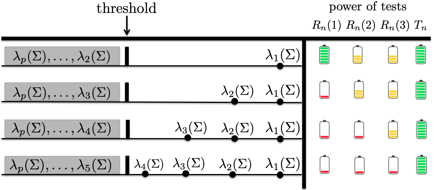
Figure 1: A conceptual comparison of the proposed statistic $T_{n}$ with $R_{n}(\kappa)$ for $\kappa=1,2,3$ in detecting four instances of $\mathsf{H}_{1,n}$. Green cells correspond to cases where a test is expected to have power approaching 1 as $n\to\infty$. Yellow cells correspond to cases where $R_{n}(\kappa)$ may have power approaching 1 as $n\to\infty$, but the power may be reduced from taking a maximum over several gap ratios. Red cells correspond to cases where $R_{n}(\kappa)$ is not expected to have power approaching 1 as $n\to\infty$.

Direct scale estimation. Based on the limitations of gap ratios, we propose a different approach, which is to construct a direct estimate $\widehat{\sigma}_{n}$ for the unknown scale of $\lambda_{1}(\widehat{\mathbf{\Sigma}})-\lambda_{2}(\widehat{\mathbf{\Sigma}})$, and use a test statistic of the form

$$T_{n}=\frac{n^{2/3}}{\widehat{\sigma}_{n}}\big{(}\lambda_{1}(\widehat{\mathbf{\Sigma}})-\lambda_{2}(\widehat{\mathbf{\Sigma}})\big{)}.$$ (1.7)

Although this statistic may appear simple at first sight, estimating the scale of $\lambda_{1}(\widehat{\mathbf{\Sigma}})-\lambda_{2}(\widehat{\mathbf{\Sigma}})$ is a challenging problem. As a matter of fact, we are not aware of any consistency guarantees for scale estimates of $\lambda_{1}(\widehat{\mathbf{\Sigma}})-\lambda_{2}(\widehat{\mathbf{\Sigma}})$ in settings like those considered here, but there are some estimates that have been proposed without guarantees [12, 46]. In Section 3, we propose a new method for this scale estimation problem, and in Proposition 1 we establish its consistency within the subcritical regime. Consequently, it is not necessary for us to rely on gap ratios, and the proposed test statistic $T_{n}$ is able to avoid the power losses associated with the statistic $R_{n}(\kappa)$ discussed earlier. Furthermore, in Section 7.2, we confirm that this power advantage holds in simulations across a range of settings, and we present a real data example in which $T_{n}$ yields smaller p-values than $R_{n}(\kappa)$. More generally, considering that $R_{n}(\kappa)$ has been extensively used in applications [e.g. 25, 11, 42, 31] and has been widely embraced in theoretical works [18, 38, 17], the statistic $T_{n}$ may have benefits that extend beyond the scope of the problem (1.5).

1.4 A consistent bootstrap for the subcritical regime

In recent years, there has been growing interest in bootstrapping statistics that depend on the eigenvalues of $\widehat{\mathbf{\Sigma}}$ in high-dimensional settings [e.g. 24, 19, 40, 30, 16, 52, 55, 56]. Much of this interest is motivated by the fact that bootstrap methods allow the distributions of many types of statistics to be approximated in a user-friendly and unified way—which can bypass the inconveniences of working with intricate asymptotic formulas on a case-by-case basis. Consequently, this flexibility provides practitioners with greater freedom to explore a wider range of statistics for developing new inference procedures.

However, in spite of the potential benefits of bootstrap methods, there are currently no theoretically-supported methods for bootstrapping functionals of the leading sample eigenvalues when the subcritical regime holds. This state of affairs can be attributed to the fact that the behavior of $\lambda_{1}(\widehat{\mathbf{\Sigma}}),\dots,\lambda_{k}(\widehat{\mathbf{\Sigma}})$ for fixed $k\geq 1$ depends heavily on which regime the model occupies. More specifically, because bootstrap methods are based on using an estimated model to generate simulated data, they are unlikely to work for statistics depending on $\lambda_{1}(\widehat{\mathbf{\Sigma}}),\dots,\lambda_{k}(\widehat{\mathbf{\Sigma}})$ if the estimated model is in the wrong regime.

To deal with this challenge, we apply our proposed test to the problem (1.5), and if $\mathsf{H}_{0,n}$ is not rejected, then we generate data from a “bootstrap world” that is designed to satisfy an approximate version of $\mathsf{H}_{0,n}$. In particular, the population eigenvalues in the bootstrap world are constructed so that they are upper bounded by an estimate of $1/[(1+\varepsilon)\xi_{n,1}]$, which is detailed in Section 3. Another key idea in designing the bootstrap world is to take advantage of a fundamental universality property of $\lambda_{1}(\widehat{\mathbf{\Sigma}}),\dots,\lambda_{k}(\widehat{\mathbf{\Sigma}})$ that holds in the subcritical regime. Namely, the joint distribution of $\lambda_{1}(\widehat{\mathbf{\Sigma}}),\dots,\lambda_{k}(\widehat{\mathbf{\Sigma}})$ is asymptotically the same as if the data in the real world are generated from the Gaussian distribution $\mathcal{N}(0,\mathbb{\Lambda})$, where $\mathbb{\Lambda}=\textup{diag}(\lambda_{1}(\mathbf{\Sigma}),\dots,\lambda_{p}(\mathbf{\Sigma}))$ [34, 53]. Accordingly, our proposed bootstrap method generates data from a fitted Gaussian distribution $\mathcal{N}(0,\tilde{\mathbb{\Lambda}})$, where $\tilde{\mathbb{\Lambda}}$ is a specially designed estimate of $\mathbb{\Lambda}$ that approximately conforms with the subcritical regime.

1.5 Outline

After laying out some technical preliminaries and assumptions in Section 2, we describe our proposed testing procedure in Section 3. Our theoretical results under the null and alternative hypothesis are respectively given in Sections 4 and 5. Next, in Section 6, we cover a methodological application to bootstrapping functionals of the leading sample eigenvalues. Numerical results involving both simulated data and financial data are presented in Section 7. Lastly, all proofs are deferred to Section 8.

2 Preliminaries and setup

Let $\mathbb{Y}\in\mathbb{R}^{n\times p}$ be a random data matrix whose rows consist of $n$ centered i.i.d. observations in $\mathbb{R}^{p}$. The associated sample covariance matrix is defined as

$$\widehat{\mathbf{\Sigma}}=\frac{1}{n}\mathbb{Y}^{\top}\mathbb{Y}$$ (2.1)

and its population counterpart is

$$\mathbf{\Sigma}=\mathbb{E}(\widehat{\mathbf{\Sigma}}).$$ (2.2)

In addition, define the $n\times n$ companion matrix associated with $\widehat{\mathbf{\Sigma}}$ as

$$\widehat{\underline{\mathbf{\Sigma}}}=\frac{1}{n}\mathbb{Y}\mathbb{Y}^{\top}.$$ (2.3)

For any real $p\times p$ symmetric matrix $\mathbf{A}$, let $F^{\mathbf{A}}$ denote the empirical spectral distribution function of $\mathbf{A}$, which satisfies

$$F^{\mathbb{A}}(t)=\frac{1}{p}\sum_{j=1}^{p}1\{\lambda_{j}(\mathbb{A})\leq t\}$$

for any $t\in\mathbb{R}$, where $1\{\cdot\}$ is an indicator function. In the particular case when $\mathbb{A}=\mathbf{\Sigma}$, we write

$$H_{n}=F^{\mathbf{\Sigma}}.$$

Stieltjes transforms and related parameters. For any distribution $F$, we denote its Stieltjes transform by

$$s_{F}(z)=\int\frac{1}{\lambda-z}dF(\lambda),\quad z\in\mathbb{C}^{+}=\{z\in\mathbb{C}:\operatorname{Im}(z)>0\}.$$

We use the notation $\underline{s}_{n}^{0}=s_{\underline{F}^{y_{n},H_{n}}},$ where $\underline{s}_{n}^{0}$ characterizes the distribution $\underline{F}^{y_{n},H_{n}}$, and is the unique solution to the equation

$$z=-\frac{1}{\underline{s}_{n}^{0}(z)}+y_{n}\int\frac{\lambda}{1+\underline{s}_{n}^{0}(z)\lambda}dH_{n}(\lambda),\quad z\in\mathbb{C}^{+},$$ (2.4)

where $y_{n}=p/n$ is the dimension-to-sample-size ratio. Further background on this equation and the characterization of the distribution $\underline{F}^{y_{n},H_{n}}$ can be found in [34, 54]. The rightmost endpoint of the support of the distribution $\underline{F}^{y_{n},H_{n}}$ is denoted by $r_{n}$ and is given by the formula [34, Lemma 2.5-2.6],

$$r_{n}=\frac{1}{\xi_{n,0}}\left(1+y_{n}\int\frac{\lambda\xi_{n,0}}{1-\lambda\xi_{n,0}}dH_{n}(\lambda)\right).$$ (2.5)

The critical parameter $\xi_{n,0}$ is also related to $\underline{s}_{n}^{0}$ and $r_{n}$ through the relation

$$\xi_{n,0}=-\lim_{\eta\to 0}\underline{s}_{n}^{0}(r_{n}+i\eta)=-\underline{s}_{n}^{0}(r_{n}),$$ (2.6)

which was established in [50]. Furthermore, the parameter $\xi_{n,0}$ is needed to define the scale parameter $\sigma_{n}$ for the leading sample eigengap $\lambda_{1}(\widehat{\mathbf{\Sigma}})-\lambda_{2}(\widehat{\mathbf{\Sigma}})$ in the subcritical regime through the formula

$$\sigma_{n}^{3}=\frac{1}{\xi_{n,0}^{3}}\bigg{(}1+y_{n}\int\Big{(}\frac{\lambda\xi_{n,0}}{1-\lambda\xi_{n,0}}\Big{)}^{3}dH_{n}(\lambda)\bigg{)}.$$ (2.7)

The interpretation of $\sigma_{n}$ as a scale parameter arises from the following fundamental result [10, 38, 34]: If the subcritical regime holds within the data-generating model given by (A1), (A2), and (A3) below, then for any fixed number $d\geq 1$, the random vector $\frac{n^{2/3}}{\sigma_{n}}(\lambda_{j}(\widehat{\mathbf{\Sigma}})-r_{n})_{1\leq j\leq d}$ converges in distribution to a $d$-dimensional Tracy-Widom distribution, as defined below.

The multivariate Tracy-Widom distribution. Let ${\bf{G}}\in\mathbb{R}^{N\times N}$ be a random matrix with i.i.d. $\mathcal{N}(0,1)$ entries, and let ${\bf{W}}=\frac{1}{\sqrt{2}}({\bf{G}}+{\bf{G}}^{\top})$, which is commonly referred to as a Wigner or GOE$(N)$ matrix. For any fixed $d\geq 1$, it is known that as $N\to\infty$, the random vector $N^{2/3}(\lambda_{j}(\mathbf{W})-2)_{1\leq j\leq d}$ has a weak limit, which is referred to as the $d$-dimensional Tracy-Widom distribution. In particular, this definition shows that the $d$-dimensional Tracy-Widom distribution can be numerically approximated by generating GOE$(N)$ matrices for large $N$.  

Data-generating model. Throughout the paper, our work will be based on a data-generating model that is defined by the following conditions.

1. There is a number $y\in(0,\infty)\setminus\{1\}$ such that $y_{n}=p/n$ satisfies $\lim_{n\to\infty}y_{n}=y$.

2. The data matrix $\mathbb{Y}\in\mathbb{R}^{n\times p}$ has the form $\mathbb{Y}=\mathbb{X}\mathbf{\Sigma}^{1/2}$, where the matrix $\mathbb{X}$ is the upper-left $n\times p$ block of a doubly-infinite array of i.i.d. random variables $\{x_{ij}:i\geq 1,j\geq 1\}$ such that $\mathbb{E}(x_{11})=0,\mathbb{E}(x_{11}^{2})=1$ and $\sup_{q\geq 1}q^{-1/\beta}(\mathbb{E}|x_{11}|^{q})^{1/q}<\infty$ for some $\beta>0$.

3. As $n\to\infty$, the distribution $H_{n}$ has a weak limit $H$. Also, the support of $H$ is a finite union of closed intervals in $(0,\infty)$, and there is a fixed compact interval in $(0,\infty)$ containing the support of $H_{n}$ for all large $n$.

3 Testing procedure

Before formally defining our testing procedure, we will assemble estimators for $\xi_{n,0}$, $\xi_{n,1}$, $H_{n}$, and $\sigma_{n}$ in the following three paragraphs.

Estimation of $\xi_{n,0}$ and $\xi_{n,1}$. Recall the formula $\xi_{n,0}=-\underline{s}_{n}^{0}(r_{n})$ from equation (2.6). Since $r_{n}$ approximately corresponds to the right edge of the limiting bulk sample spectrum, it is naturally estimated by $\lambda_{1}(\widehat{\mathbf{\Sigma}})$. Meanwhile, the Stieltjes transform $\underline{s}_{n}^{0}$ is the limit of $\underline{s}_{n}=s_{F^{\underline{\widehat{\mathbf{\Sigma}}}}}$, but because the latter function is not defined at $\lambda_{1}(\widehat{\mathbf{\Sigma}})$, we will use the modified version

$$\tilde{}\underline{s}_{n}(z)=\frac{1}{n}\sum\limits_{j=2}^{n}\frac{1}{\lambda_{j}(\underline{\widehat{\mathbf{\Sigma}}})-z},\quad z\in\mathbb{C}\setminus[\lambda_{n}(\underline{\widehat{\mathbf{\Sigma}}}),\lambda_{2}(\underline{\widehat{\mathbf{\Sigma}}})].$$ (3.1)

Likewise, we define the estimate

$$\widehat{\xi}_{n}=\begin{cases}-\tilde{}\underline{s}_{n}(\lambda_{1}(\widehat{\mathbf{\Sigma}}))&\textnormal{ if }\lambda_{1}(\widehat{\mathbf{\Sigma}})>\lambda_{2}(\widehat{\mathbf{\Sigma}}),\\ -\tilde{\underline{s}}_{n}(\lambda_{1}(\widehat{\mathbf{\Sigma}})+1)&\textnormal{ if }\lambda_{1}(\widehat{\mathbf{\Sigma}})=\lambda_{2}(\widehat{\mathbf{\Sigma}}).\end{cases}$$ (3.2)

We have intentionally chosen to write $\widehat{\xi}_{n}$ rather than $\widehat{\xi}_{n,0}$, because the parameters $\xi_{n,0}$ and $\xi_{n,1}$ are sufficiently close asymptotically that $\widehat{\xi}_{n}$ may be regarded as an estimate of either of them. (It will be shown in Lemma 4 that $0<\xi_{n,1}-\xi_{n,0}\lesssim 1/p$.)

Estimation of $H_{n}$. We estimate the empirical spectral distribution $H_{n}$ using a modified version of the QuEST procedure (see [36, 37]). The modification is needed to ensure that the estimate for $H_{n}$ conforms with the subcritical regime, and this is achieved with specially designed truncation. To be precise, for each $j=1,\dots,p$, let $\tilde{\lambda}_{j,Q}$ be the $j/p$ quantile of the QuEST estimator for $H_{n}$, and let

$$\tilde{\lambda}_{j}=\tilde{\lambda}_{j,Q}\wedge\textstyle\frac{1}{\widehat{\xi}_{n}(1+\varepsilon)}\quad 1\leq j\leq p.$$ (3.3)

In turn, our estimate of $H_{n}$ is defined as

$$\tilde{H}_{n}(t)=\frac{1}{p}\sum\limits_{j=1}^{p}1\{\tilde{\lambda}_{j}\leq t\}$$ (3.4)

for all real $t$.

Estimation of $\sigma_{n}$. Based on the formula (2.7) for the scale parameter $\sigma_{n}$, we estimate it by directly substituting the estimates for $\xi_{n,0}$ and $H_{n}$ constructed above. That is, we define

$$\widehat{\sigma}_{n}^{3}=\frac{1}{\widehat{\xi}_{n}^{3}}\bigg{(}1+y_{n}\int\bigg{(}\frac{\lambda\widehat{\xi}_{n}}{1-\lambda\widehat{\xi}_{n}}\bigg{)}^{3}d\tilde{H}_{n}(\lambda)\bigg{)}.$$ (3.5)

Test statistic. To test the null hypothesis (1.5) for a specified value of $\varepsilon\in(0,1)$, we propose to use the statistic

$$T_{n}=\frac{n^{2/3}}{\widehat{\sigma}_{n}}\big{(}\lambda_{1}(\widehat{\mathbf{\Sigma}})-\lambda_{2}(\widehat{\mathbf{\Sigma}})\big{)}.$$

Note that the statistic depends on $\varepsilon$ through the eigenvalue estimates in (3.3) that underpin $\tilde{H}_{n}$ and $\widehat{\sigma}_{n}$.

To specify the rejection criterion, let $(\zeta,\zeta^{\prime})$ follow a two-dimensional Tracy-Widom distribution and let $q_{1-\alpha}$ be the $(1-\alpha)$-quantile of the difference $\zeta-\zeta^{\prime}$. For a prescribed level $\alpha$, the proposed testing procedure rejects the null hypothesis in (1.5) when

$$T_{n}>q_{1-\alpha}.$$ (3.6)

4 Theoretical results under the null hypothesis

In this section, we establish the limiting null distribution of the proposed test statistic $T_{n}$ in Theorem 1. Since this theorem hinges on the performance of the estimates $\widehat{\xi}_{n}$, $\widehat{\sigma}_{n}$, and $\tilde{H}_{n}$, we first demonstrate their consistency in the following proposition. For the purpose of stating this result, convergence in probability and distribution are respectively denoted by $\xrightarrow{\mathbb{P}}$ and $\stackrel{{\scriptstyle\mathcal{D}}}{{\to}}$.

Proposition 1.

Suppose that assumptions (A1)-(A3) are satisfied and that $\mathsf{H}_{0,n}$ holds for all large $n$. Then, the estimates $\widehat{\xi}_{n}$, $\widehat{\sigma}_{n}$, and $\tilde{H}_{n}$ satisfy the following limits as $n\to\infty$

$$\widehat{\xi}_{n}-\xi_{n,k} \xrightarrow{\mathbb{P}}0\textup{ \ \ for }k\in\{0,1\},$$ (a)

$$\tilde{H}_{n} \stackrel{{\scriptstyle\mathcal{D}}}{{\to}}H\textnormal{ in probability},$$ (b)

$$\frac{\widehat{\sigma}_{n}}{\sigma_{n}} \xrightarrow{\mathbb{P}}1.$$ (c)

These three limits are proven in Section 8.2.1. The limit $\widehat{\sigma}_{n}/\sigma_{n}\xrightarrow{\mathbb{P}}1$ may be of independent interest, since consistent estimation of $\sigma_{n}$ has not previously been established.

The following theorem is the main result of this section and ensures that the rejection criterion (3.6) corresponds to a test with an asymptotically controlled level.

Theorem 1.

If (A1)-(A3) are satisfied and $\mathsf{H}_{0,n}$ holds for all large $n$, then as $n\to\infty$,

$$T_{n}\stackrel{{\scriptstyle\mathcal{D}}}{{\to}}\zeta-\zeta^{\prime},$$

where $(\zeta,\zeta^{\prime})$ follows a two-dimensional Tracy-Widom distribution. In particular, for any fixed $\alpha\in(0,1)$, we have $\mathbb{P}(T_{n}>q_{1-\alpha})\to\alpha$ as $n\to\infty$.

Theorem 1 follows by combining Slutsky’s theorem with Proposition 1(c) and the limit (8.5) given later. Thus, the primary technical challenge in establishing Theorem 1 lies in proving Proposition 1.

As an added benefit of our work so far, it is possible to develop confidence intervals for the parameters $\lambda_{1}(\mathbf{\Sigma})$ and $r_{n}$. For this purpose, define $\widehat{\varepsilon}$ as the smallest $\varepsilon>0$ for which $\mathsf{H}_{0,n}$ is rejected based on the statistic $T_{n}=T_{n}(\varepsilon)$ at a fixed nominal level $\alpha$. More formally, since $T_{n}(\varepsilon)$ is a non-decreasing function of $\varepsilon$, we may define $\widehat{\varepsilon}=T_{n}^{-1}(q_{1-\alpha}),$ where $T_{n}^{-1}(q)=\inf\{\varepsilon>0:T_{n}(\varepsilon)\geq q\}$ denotes the generalized inverse.

Corollary 1.

Fix any $\alpha\in(0,1)$. If assumptions (A1)-(A3) are satisfied and if $\mathsf{H}_{0,n}$ holds for all large $n$, then

$$\mathbb{P}\bigg{(}\lambda_{1}(\mathbf{\Sigma})\in\Big{(}\textstyle\frac{1}{(1+\widehat{\varepsilon})\widehat{\xi}_{n}},\infty\Big{)}\bigg{)}\geq 1-\alpha+o(1)$$

and

$$\mathbb{P}\bigg{(}r_{n}\in\Big{[}\lambda_{1}(\widehat{\mathbf{\Sigma}})\pm\textstyle\frac{q_{\alpha/2}^{\prime}\widehat{\sigma}_{n}}{n^{2/3}}\Big{]}\bigg{)}=1-\alpha+o(1).$$

where $q_{\alpha/2}^{\prime}$ denotes the $(\alpha/2)$-quantile of the one-dimensional Tracy-Widom distribution.

The proof of Corollary 1 is given in Section 8.2.

5 Theoretical results under alternative hypotheses

In this section, we study the power of the proposed test under alternative hypotheses that are particular instances of $\mathsf{H}_{1,n}$, defined in (1.5). These instances specify the particular number of supercritical population eigenvalues, whereas $\mathsf{H}_{1,n}$ allows for various numbers of such eigenvalues. In detail, if $\varepsilon\in(0,1)$ and $K\geq 1$ are fixed with respect to $n$, then the alternative $\mathsf{H}_{1,n}(K)$ defined below has the interpretation that there are exactly $K$ supercritical population eigenvalues,

$$\small\mathsf{H}_{1,n}(K):\ \ \lambda_{j}(\mathbf{\Sigma})\geq\frac{1}{(1-\varepsilon)\xi_{n,j}}\textup{ \ for \ $j=1,\dots,K$, \ \ \ \ and \ \ \ \ }\lambda_{K+1}(\mathbf{\Sigma})\leq\frac{1}{(1+\varepsilon)\xi_{n,K}}.$$ (5.1)

Before stating the main result on power consistency, it is worth pointing out a connection between the hypothesis $\mathsf{H}_{1,n}(K)$ and a standard formulation of supercritical eigenvalues in the random matrix theory literature. For any $\beta\not\in\textup{supp}(H)$, define the function

$$\psi(\beta)=\beta+y\beta\int\frac{\lambda}{\beta-\lambda}dH(\lambda).$$ (5.2)

The derivative $\psi^{\prime}(\beta)$ exists for all $\beta\not\in\operatorname{supp}(H)$, and for convenience of presentation, we define $\psi^{\prime}(\beta)=0$ for all $\beta\in\operatorname{supp}(H)$. Conceptually, the derivative is important, because the condition

$$\psi^{\prime}(\lambda_{j}(\mathbf{\Sigma}))>0$$

is often interpreted to mean that $\lambda_{j}(\mathbf{\Sigma})$ is supercritical [39, 57, 27]. As a concrete example, note that in a simple model where $\mathbf{\Sigma}=\textup{diag}(\lambda_{1}(\mathbf{\Sigma}),\dots,\lambda_{K}(\mathbf{\Sigma}),1,\dots,1)$ and $H$ is the pointmass at 1, it can be verified by direct calculation that $\psi^{\prime}(\lambda_{j}(\mathbf{\Sigma}))>0$ is equivalent to $\lambda_{j}(\mathbf{\Sigma})>1+\sqrt{y}$. The main point of Proposition 2 below is that it gives general conditions under which $\mathsf{H}_{1,n}(K)$ implies that $\psi^{\prime}(\lambda_{j}(\mathbf{\Sigma}))>0$ holds for all $1\leq j\leq K$. Its proof is given in Section 8.4.

Proposition 2.

Suppose that (A1) and (A3) hold. Also, suppose that $\lambda_{1}(\mathbf{\Sigma})>\dots>\lambda_{K}(\mathbf{\Sigma})$ are fixed with respect to $n$, and that $\mathsf{H}_{1,n}(K)$ holds for all large $n$. Then, the condition $\psi^{\prime}(\lambda_{j}(\mathbf{\Sigma}))>0$ holds for all $1\leq j\leq K.$

The following theorem establishes the power consistency of the proposed test, and is proved in Section 8.4.

Theorem 2.

Suppose that (A1)-(A3) hold. Also, suppose that $\lambda_{1}(\mathbf{\Sigma})>\dots>\lambda_{K}(\mathbf{\Sigma})$ are fixed with respect to $n$, and that $\mathsf{H}_{1,n}(K)$ holds for all large $n$. Then,

$$\lim_{n\to\infty}\mathbb{P}\left(T_{n}>q_{1-\alpha}\right)=1.$$

If the null hypothesis in (1.5) is rejected, it is natural to ask for the number of supercritical eigenvalues in the underlying model. Indeed, this quantity is of fundamental interest in the literature on high-dimensional sample covariance matrices [e.g. 43, 45, 15, 33, 12]. To illustrate the versatility of our testing approach, we will show how it can be adapted to this task. Specifically, if $\mathsf{H}_{1,n}(K)$ holds for some unknown value of $K\geq 1$, then a consistent estimate of $K$ can be constructed as follows.

For each $j=1,\dots,p-1$, define the $j$th gap statistic

$$\frac{n^{2/3}}{\widehat{\sigma}_{n}}\left(\lambda_{j}(\widehat{\mathbf{\Sigma}})-\lambda_{j+1}(\widehat{\mathbf{\Sigma}})\right),$$

which specializes to $T_{n}$ when $j=1$. The estimate of $K$ is then defined by

$$\widehat{K}_{n}=\min\{k\in\mathbb{N}:T_{n,k}<t_{n}\}-1,$$

where $t_{n}$ is a suitably chosen threshold. The next result shows that any choice of $t_{n}$ satisfying $t_{n}\asymp n^{\nu}$ with $0<\nu<2/3$ leads to a consistent estimate of $K$.

Corollary 2.

If the conditions of Theorem 2 hold, and if $t_{n}\asymp n^{\nu}$ with $0<\nu<2/3$, then

$$\lim_{n\to\infty}\mathbb{P}(\widehat{K}_{n}=K)=1.$$

This result is proven in Section 8.4.

6 A consistent bootstrap for the subcritical regime

In this section, we introduce a new bootstrap method for approximating the distributions of functionals of leading sample eigenvalues in the subcritical regime. That is, the statistics of interest $\widehat{\theta}$ have the form

$$\widehat{\theta}=\varphi(\lambda_{1}(\widehat{\mathbf{\Sigma}}),\dots,\lambda_{k}(\widehat{\mathbf{\Sigma}})),$$

where $\varphi:\mathbb{R}^{k}\to\mathbb{R}^{m}$ is a generic function, and $k,m\geq 1$ are fixed integers. As has been highlighted elsewhere in the literature [19], the non-parametric bootstrap based on sampling with replacement often fails to approximate the distributions of such statistics in the subcritical regime. The bootstrap method proposed here provides a solution to this problem.

At a conceptual level, the method is based on three ingredients. The first ingredient is the test from Section 3, which guides the user to determine whether or not a bootstrap for the subcritical regime is appropriate. The second ingredient is a fundamental universality result, which ensures that within the subcritical regime, the sample eigenvalues $\lambda_{1}(\widehat{\mathbf{\Sigma}}),\dots,\lambda_{k}(\widehat{\mathbf{\Sigma}})$ behave asymptotically as if the data were generated from the Gaussian distribution $\mathcal{N}(\mathbf{0},\mathbf{\Lambda})$, where $\mathbb{\Lambda}=\textup{diag}(\lambda_{1}(\mathbf{\Sigma}),\dots,\lambda_{p}(\mathbf{\Sigma}))$ [34, 53]. The third ingredient is the matrix of truncated eigenvalue estimates $\tilde{\mathbf{\Lambda}}=\textup{diag}(\tilde{\lambda}_{1},\dots,\tilde{\lambda}_{p})$ defined in (3.3), which is specially designed to conform with an approximate version of the subcritical condition. Altogether, the method generates bootstrap data from the fitted Gaussian distribution $\mathcal{N}(\mathbf{0},\tilde{\mathbf{\Lambda}})$, as shown in the following algorithm.

Algorithm 1 Bootstrap method for the subcritical regime

the matrix $\tilde{\mathbf{\Lambda}}$.

for $b=1$ to $B$ do

  Generate independent random vectors $\mathbf{y}_{1}^{\star},\ldots,\mathbf{y}_{n}^{\star}$ from $\mathcal{N}(\mathbf{0},\tilde{\mathbf{\Lambda}})$.

  Compute the sample covariance matrix $\widehat{\mathbf{\Sigma}}^{\star}=\frac{1}{n}\sum\limits_{i=1}^{n}\mathbf{y}_{i}^{\star}(\mathbf{y}_{i}^{\star})^{\top}$.

  Compute the statistic $\widehat{\theta}^{\star}=\varphi(\lambda_{1}(\widehat{\mathbf{\Sigma}}^{\star}),\dots,\lambda_{k}(\widehat{\mathbf{\Sigma}}^{\star}))$.

end for

Output: Empirical distribution of $\widehat{\theta}_{1}^{\star},\dots,\widehat{\theta}_{B}^{\star}$.

While the outward appearance of the algorithm is straightforward, this appearance conceals two major challenges that the method overcomes. These are determining whether or not the subcritical regime holds, and estimating $\lambda_{1}(\mathbf{\Sigma}),\dots,\lambda_{p}(\mathbf{\Sigma})$ in a way that respects the subcritical regime. So, in essence, the simple form of Algorithm 1 is made possible by the insights that are embedded in the design of the test $T_{n}$ and the eigenvalue estimates $\tilde{\boldsymbol{\Lambda}}$.

Consistency. To formulate a consistency guarantee for the proposed bootstrap, let $d$ denote any metric on the space of probability distributions on $\mathbb{R}^{m}$ whose topology coincides with that of weak convergence. For example, it suffices to take $d$ to be the Lévy-Prohorov metric. Next, let $\tilde{\xi}_{n,0}\in(0,1/\tilde{\lambda}_{1})$ be the unique value that solves the equation

$$\frac{1}{p}\sum_{j=1}^{p}\bigg{(}\frac{\tilde{\lambda}_{j}\tilde{\xi}_{n,0}}{1-\tilde{\lambda}_{j}\tilde{\xi}_{n,0}}\bigg{)}^{2}=\frac{n}{p}.$$ (6.1)

Also, define

$$\tilde{r}_{n} =\frac{1}{\tilde{\xi}_{n,0}}\bigg{(}1+y_{n}\int\frac{\lambda\tilde{\xi}_{n,0}}{1-\lambda\tilde{\xi}_{n,0}}d\tilde{H}_{n}(\lambda)\bigg{)},$$ (6.2)

$$\tilde{\sigma}_{n}^{3} =\frac{1}{\tilde{\xi}_{n,0}^{3}}\bigg{(}1+y_{n}\int\bigg{(}\frac{\lambda\tilde{\xi}_{n,0}}{1-\lambda\tilde{\xi}_{n,0}}\bigg{)}^{3}d\tilde{H}_{n}(\lambda)\bigg{)}.$$ (6.3)

These quantities only serve a formal purpose, which is to normalize $\lambda_{1}(\widehat{\mathbf{\Sigma}}^{\star}),\dots,\lambda_{k}(\widehat{\mathbf{\Sigma}}^{\star})$ so that their fluctuations can be theoretically compared with those of $\lambda_{1}(\widehat{\mathbf{\Sigma}}),\dots,\lambda_{k}(\widehat{\mathbf{\Sigma}})$. In detail, for any fixed integers $k,m\geq 1$ and continuous function $g:\mathbb{R}^{k}\to\mathbb{R}^{m}$, the comparison will be made between the random vectors

$$V_{n} =g\Big{(}\textstyle\frac{n^{2/3}}{\sigma_{n}}(\lambda_{1}(\widehat{\mathbf{\Sigma}})-r_{n}),\dots,\textstyle\frac{n^{2/3}}{\sigma_{n}}(\lambda_{k}(\widehat{\mathbf{\Sigma}})-r_{n})\Big{)}$$

$$V_{n}^{\star} =g\Big{(}\textstyle\frac{n^{2/3}}{\tilde{\sigma}}(\lambda_{1}(\widehat{\mathbf{\Sigma}}^{\star})-\tilde{r}_{n}),\dots,\textstyle\frac{n^{2/3}}{\tilde{\sigma}}(\lambda_{k}(\widehat{\mathbf{\Sigma}}^{\star})-\tilde{r}_{n})\Big{)}.$$

Lastly, in order to refer to the conditional distribution of $V_{n}^{\star}$ given the original matrix of observations $\mathbf{Y}$, we write $\mathcal{L}\left(V_{n}^{\star}|\mathbf{Y}\right).$ With this notation in hand, we are now in position to state the following bootstrap consistency result.

Theorem 3.

If $\mathsf{H}_{0,n}$ holds for all large $n$ and (A1)-(A3) are satisfied, then as $n\to\infty$

$$d\!\left(\mathcal{L}\left(V_{n}^{\star}|\mathbf{Y}\right),\mathcal{L}\left(V_{n}\right)\right)\xrightarrow{\mathbb{P}}0.$$

From a practical standpoint, it should be emphasized that the bootstrapped eigenvalues $\lambda_{1}(\widehat{\mathbf{\Sigma}}^{\star}),\dots,\lambda_{k}(\widehat{\mathbf{\Sigma}}^{\star})$ do not need to be normalized as above in order to apply Algorithm 1 to solve various inference tasks. For instance, consider the problem of estimating the bias $\mathbb{E}(\lambda_{1}(\widehat{\mathbf{\Sigma}}))-\lambda_{1}(\mathbf{\Sigma})$ of the largest sample eigenvalue. In this case, the bootstrap estimate is defined as $\mathbb{E}(\lambda_{1}(\widehat{\mathbf{\Sigma}}^{\star})|\mathbf{Y})-\tilde{\lambda}_{1}$, where the conditional expectation is numerically approximated by averaging the $B$ realizations of $\lambda_{1}(\widehat{\mathbf{\Sigma}}^{\star})$ in Algorithm 1. In the experiments presented in Section 7.2, we show that the bootstrap reliably estimates the bias across a range of conditions.

7 Numerical experiments

This section presents three collections of empirical results on the performance of the proposed methods. First, in Section 7.1 we use simulated data to compare the proposed statistic $T_{n}$ with Onatski’s statistic $R_{n}(\kappa)$ in testing $\mathsf{H}_{0,n}$. This comparison shows that both statistics have a well-controlled level, while $T_{n}$ delivers substantially higher power. Second, in Section 7.2, we look at the empirical performance of the proposed bootstrap, showing that it can accurately approximate the distributions of normalized versions of $\lambda_{1}(\widehat{\mathbf{\Sigma}})$ and $\lambda_{1}(\widehat{\mathbf{\Sigma}})-\lambda_{2}(\widehat{\mathbf{\Sigma}})$, and also accurately estimate the bias $\mathbb{E}(\lambda_{1}(\widehat{\mathbf{\Sigma}}))-\lambda_{1}(\mathbf{\Sigma})$. Lastly, in Section 7.3, we apply $T_{n}$ and $R_{n}(\kappa)$ to test $\mathsf{H}_{0,n}$ using two high-dimensional datasets derived from the stock market returns of companies in the S&P 500. In these real-data examples, $T_{n}$ produces smaller p-values, which aligns with the power advantage observed in the simulations from Section 7.1. Throughout all of the experiments, we always put $\varepsilon=0.2$ in the definition of $\mathsf{H}_{0,n}$ and the alternatives.

7.1 Testing the subcritical condition

To generate data under the null $\mathsf{H}_{0,n}$ and the alternatives $\mathsf{H}_{1,n}(K)$ with $K\in\{1,2\}$, we used the model given in (A2) with $(n,p)=(600,400)$ and varying choices of the leading eigenvalues of $\mathbf{\Sigma}$.

Experiments with varying $\lambda_{1}(\mathbf{\Sigma})$. First, we describe a subset of simulations in which only $\lambda_{1}(\mathbf{\Sigma})$ was varied over a grid of values in the interval $[1,3.5]$, while keeping $\lambda_{2}(\mathbf{\Sigma}),\dots,\lambda_{p}(\mathbf{\Sigma})$ fixed. This was done using $\mathbf{\Sigma}=\textup{diag}(\lambda_{1}(\mathbf{\Sigma}),\dots,\lambda_{p}(\mathbf{\Sigma}))$ and choosing the eigenvalues $\lambda_{2}(\mathbf{\Sigma}),\dots,\lambda_{p}(\mathbf{\Sigma})$ to have two types of structures, that that we refer to as the ‘spiked spectrum’ and ‘decaying spectrum’. In the case of the spiked spectrum, we put $\lambda_{j}(\mathbf{\Sigma})=1$ for all $j=2,\dots,p$, while in the case of the decaying spectrum, we put $\lambda_{j}(\mathbf{\Sigma})=1$ for $j\in\{2,\dots,151\}$ and $\lambda_{j}(\mathbf{\Sigma})=j^{-c}$ for $j\in\{152,\dots,p\}$ with $c\in\{0.5,1\}$. For each setting of $\mathbf{\Sigma}$, we generated 800 realizations of the data matrix $\mathbf{Y}=\mathbf{X}\mathbf{\Sigma}^{1/2}$ with $\mathbf{X}\in\mathbb{R}^{n\times p}$ having i.i.d. entries, and taking the random variable $x_{11}$ to follow either a $\mathcal{N}(0,1)$ distribution or a standardized $t_{10}$ distribution. Next, for each realization of $\mathbf{Y}$, we computed test statistics $T_{n}$ and $R_{n}(\kappa)$ with $\kappa\in\{1,10\}$, and recorded whether or not $\mathsf{H}_{0,n}$ was rejected at a nominal level of $\alpha=0.05$. We refer to the proportion of rejections occurring among these 800 trials as the rejection probability. Note also that the critical value for $R_{n}(\kappa)$ is given by the $(1-\alpha)$-quantile of the random variable $\max_{1\leq j\leq\kappa}\{(\zeta_{j}-\zeta_{j+1})/(\zeta_{j+1}-\zeta_{j+2})\}$, where $(\zeta_{1},\dots,\zeta_{\kappa+2})$ follows a $(\kappa+2)$-dimensional Tracy-Widom distribution.

The results are displayed in Figure 2 by plotting the rejection probabilities of the tests as a function of $\lambda_{1}(\mathbf{\Sigma})$. The four panels correspond to different model configurations that are indicated in the caption. As $\lambda_{1}(\mathbf{\Sigma})$ increases from $1$ to 3.5 in each panel, there is a transition from $\mathsf{H}_{0,n}$ to $\mathsf{H}_{1,n}(1)$, and the range of values of $\lambda_{1}(\mathbf{\Sigma})$ corresponding to each hypothesis are marked below the x-axis. Under the null hypothesis $\mathsf{H}_{0,n}$, all three statistics produce rejection probabilities that agree closely with the nominal level of $\alpha=0.05$. On the other hand, when $\mathsf{H}_{1,n}(1)$ holds, we see that $T_{n}$ has substantially higher power than $R_{n}(1)$ and $R_{n}(10)$.

There are a few more aspects of the results in Figure 2 to discuss. First, the ideal choice of $\kappa$ for detecting $\mathsf{H}_{1,n}(1)$ with the statistic $R_{n}(\kappa)$ is $\kappa=1$, and so it is notable that even when $R_{n}(\kappa)$ is favorably tuned, the statistic $T_{n}$ still provides higher power. Second, the loss of power suffered by $R_{n}(10)$ in comparison to $R_{n}(1)$ illustrates the practical drawback of using a conservatively large value of $\kappa$ that was explained in the introduction (page 1.3). Third, the decaying spectrum violates the theoretical condition (A3), and the standardized $t_{10}$ distribution has tails that are too heavy to satisfy the moment assumptions in (A2). Thus, the results in Figure 2 show that the statistic $T_{n}$ has a scope of application that extends beyond those conditions.

\begin{overpic}[width=433.62pt]{n600_p400.pdf} \put(-6.0,35.0){\rotatebox{90.0}{rejection probability}} \put(6.0,11.5){$\alpha$} \put(9.0,-12.0){ $\leftarrow\!\!\mathsf{H}_{0,n}\!\!\rightarrow$ } \put(53.0,-12.0){ $\xleftarrow{\ \ \ \ \ \ }\mathsf{H}_{1,n}(1)\xrightarrow{\ \ \ \ }$ } \put(35.0,-4.0){ value of $\lambda_{1}(\mathbf{\Sigma})$ } \end{overpic}

\begin{overpic}[width=433.62pt]{n600_p400_nonnormal.pdf} \put(-6.0,35.0){\rotatebox{90.0}{rejection probability}} \put(6.0,11.5){$\alpha$} \put(9.0,-12.0){ $\leftarrow\!\!\mathsf{H}_{0,n}\!\!\rightarrow$ } \put(53.0,-12.0){ $\xleftarrow{\ \ \ \ \ \ }\mathsf{H}_{1,n}(1)\xrightarrow{\ \ \ \ }$ } \put(35.0,-4.0){ value of $\lambda_{1}(\mathbf{\Sigma})$ } \end{overpic}

\begin{overpic}[width=433.62pt]{poly_decay_1.pdf} \put(-6.0,35.0){\rotatebox{90.0}{rejection probability}} \put(6.0,11.5){$\alpha$} \put(7.0,-12.0){ $\footnotesize\shortleftarrow\!\!\displaystyle\mathsf{H}_{0,n}\!\!\!\!\footnotesize\shortrightarrow$ } \put(40.0,-12.0){ $\xleftarrow{\ \ \ \ \ \ \ \ }\mathsf{H}_{1,n}(1)\xrightarrow{\ \ \ \ \ \ \ \ \ }$ } \put(35.0,-4.0){ value of $\lambda_{1}(\mathbf{\Sigma})$ } \end{overpic}

\begin{overpic}[width=433.62pt]{poly_decay_05.pdf} \put(-6.0,35.0){\rotatebox{90.0}{rejection probability}} \put(6.0,11.5){$\alpha$} \put(7.0,-12.0){ $\shortleftarrow\!\!\mathsf{H}_{0,n}\!\!\!\shortrightarrow$ } \put(41.0,-12.0){ $\xleftarrow{\ \ \ \ \ \ \ \ }\mathsf{H}_{1,n}(1)\xrightarrow{\ \ \ \ \ \ \ \ \ }$ } \put(35.0,-4.0){ value of $\lambda_{1}(\mathbf{\Sigma})$ } \end{overpic}

Figure 2: Rejection probabilities for the tests $T_{n}$ (triangle), $R_{n}(1)$ (diamond) and $R_{n}(10)$ (circle), plotted as a function of $\lambda_{1}(\mathbf{\Sigma})$. In each panel, the arrows below the x-axis specify the values of $\lambda_{1}(\mathbf{\Sigma})$ corresponding to $\mathsf{H}_{0,n}$ and $\mathsf{H}_{1,n}(1)$. The nominal level of $\alpha=0.05$ is marked with a horizontal line in each panel. First row: Spiked spectrum with $x_{11}\sim\mathcal{N}(0,1)$ (left panel) and $x_{11}\sim t_{10}/\sqrt{\operatorname{var}(t_{10})}$ (right panel). Second row: Decaying spectrum with $x_{11}\sim\mathcal{N}(0,1)$, and decay parameter $c=1$ (left panel) and $c=0.5$ (right panel).

Experiments with varying $\lambda_{1}(\mathbf{\Sigma}),\lambda_{2}(\mathbf{\Sigma}),\lambda_{3}(\mathbf{\Sigma})$. As an extension of the previous simulations, we compared the statistics $T_{n}$, $R_{n}(1)$ and $R_{n}(10)$ under varying choices of the leading three population eigenvalues when $\mathbf{\Sigma}=\textup{diag}(\lambda_{1}(\mathbf{\Sigma}),\lambda_{2}(\mathbf{\Sigma}),\lambda_{3}(\mathbf{\Sigma}),1,\dots,1)$ and $x_{11}\sim\mathcal{N}(0,1)$. The choices of the leading eigenvalues correspond to the hypotheses $\mathsf{H}_{0,n}$, $\mathsf{H}_{1,n}(1)$ and $\mathsf{H}_{1,n}(2)$, and are listed in Table 1. Overall, the relative performance of the statistics is similar to the previous settings—insofar as their rejection probabilities are close to the nominal level of $\alpha=0.05$ under the null, and $T_{n}$ achieves greater power under the alternatives. A distinct phenomenon shown in the boxed entries of Table 1 is that $R_{n}(1)$ fails to achieve any power under $\mathsf{H}_{1,n}(2)$, as anticipated by the discussion in the introduction (page 1.3). In particular, this illustrates the sensitivity of the statistic $R_{n}(\kappa)$ to the choice of $\kappa$.

			rejection probabilities
hypothesis	$K$	$(\lambda_{1}(\mathbf{\Sigma}),\lambda_{2}(\mathbf{\Sigma}),\lambda_{3}(\mathbf{\Sigma}))$	$T_{n}$	$R_{n}(1)$	$R_{n}(10)$
$\mathsf{H}_{0,n}$	0	$(1,1,1)$	0.05	0.05	0.04
$\mathsf{H}_{0,n}$	0	$(1.25,1.25,1.25)$	0.04	0.04	0.07
$\mathsf{H}_{0,n}$	0	$(1.25,1.25,1)$	0.06	0.07	0.06
$\mathsf{H}_{0,n}$	0	$(1.3,1.3,1.3)$	0.05	0.06	0.06
$\mathsf{H}_{0,n}$	0	$(1.3,1.3,1)$	0.05	0.06	0.06
$\mathsf{H}_{0,n}$	0	$(1.5,1.5,1.3)$	0.05	0.04	0.05
$\mathsf{H}_{0,n}$	0	$(1.5,1.5,1)$	0.06	0.05	0.05
$\mathsf{H}_{1,n}(K)$	1	$(2.5,1.5,1.3)$	0.96	0.42	0.12
$\mathsf{H}_{1,n}(K)$	1	$(3,1.5,1.3)$	1.00	0.79	0.28
$\mathsf{H}_{1,n}(K)$	1	$(3.5,1.5,1.3)$	1.00	0.97	0.46
$\mathsf{H}_{1,n}(K)$	1	$(4,1.5,1.3)$	1.00	1.00	0.66
$\mathsf{H}_{1,n}(K)$	1	$(4.5,1.5,1.3)$	1.00	1.00	0.84
$\mathsf{H}_{1,n}(K)$	1	$(5,1.5,1.3)$	1.00	1.00	0.93
$\mathsf{H}_{1,n}(K)$	2	$(4,3,1)$	1.00	$$0.00$$	0.28
$\mathsf{H}_{1,n}(K)$	2	$(5,3,1)$	1.00	$$0.00$$	0.27

Table 1: Rejection probabilities for the tests $T_{n}$, $R_{n}(1)$ and $R_{n}(10)$ under the null $\mathsf{H}_{0,n}$ and the alternatives $\mathsf{H}_{1,n}(K)$, $K\in\{1,2\}$ when $\mathbf{\Sigma}=\textup{diag}(\lambda_{1}(\mathbf{\Sigma}),\lambda_{2}(\mathbf{\Sigma}),\lambda_{3}(\mathbf{\Sigma}),1,\dots,1)$ and $x_{11}\sim\mathcal{N}(0,1)$. Recall that $K$ denotes the number of supercritical population eigenvalues, and the nominal level is $\alpha=0.05$. The boxed entries illustrate cases where $R_{n}(\kappa)$ has no power when $\kappa<K$.

7.2 Bootstrap

This subsection illustrates the performance of the proposed bootstrap method in two tasks: distributional approximation and bias estimation.

Distributional approximation. Here, we look at how well the bootstrap can approximate the distributions of the statistics

$$L_{n} =\frac{n^{2/3}}{\sigma_{n}}\big{(}\lambda_{1}(\widehat{\mathbf{\Sigma}})-r_{n}\big{)}$$ (7.1)

$$G_{n} =\frac{n^{2/3}}{\sigma_{n}}\big{(}\lambda_{1}(\widehat{\mathbf{\Sigma}})-\lambda_{2}(\widehat{\mathbf{\Sigma}})\big{)},$$ (7.2)

with respect to their means, standard deviations, and 0.95-quantiles.

Synthetic $n\times p$ data matrices of the form $\mathbf{Y}=\mathbf{X}\mathbf{\Sigma}^{1/2}$ were generated with $(n,p)=(500,300)$, and $\mathbf{X}$ having i.i.d. entries $x_{11}\sim\mathcal{N}(0,1)$ or $x_{11}\sim t_{10}/\sqrt{\operatorname{var}(t_{10})}$. The matrix $\mathbf{\Sigma}$ was chosen by considering a spectral decomposition $\mathbf{\Sigma}=\mathbf{Q}\mathbf{\Lambda}\mathbf{Q}^{\top}$, where $\mathbf{Q}$ was drawn uniformly at random from the set of $p\times p$ orthogonal matrices, and the matrix of eigenvalues $\mathbf{\Lambda}$ was taken to have the following three forms

1. $\mathbf{\Lambda}=\mathbf{I}$,

2. $\mathbf{\Lambda}=\operatorname{diag}(1.4,1.2,1,\ldots,1),$

3. $\mathbf{\Lambda}=\operatorname{diag}(1.3,1.3,1.3,1.3,1.3,1,\ldots,1)$.

For each choice of $\mathbf{\Sigma}$ and the distribution of $x_{11}$, we generated 30000 realizations of $\mathbf{Y}$, and computed the corresponding values of $L_{n}$ and $G_{n}$. The empirical means, standard deviations, and 0.95-quantiles associated with these samples were then treated as ground truth for the distributions of $L_{n}$ and $G_{n}$. For the first 600 realizations of $\mathbf{Y}$, we applied Algorithm 1 to generate $B=500$ bootstrap samples of the form $L_{n}^{\star}=\frac{n^{2/3}}{\tilde{\sigma}_{n}}\big{(}\lambda_{1}(\widehat{\mathbf{\Sigma}}^{\star})-\tilde{r}_{n}\big{)}$ and $G_{n}^{\star}=\frac{n^{2/3}}{\tilde{\sigma}_{n}}\big{(}\lambda_{1}(\widehat{\mathbf{\Sigma}}^{\star})-\lambda_{2}(\widehat{\mathbf{\Sigma}}^{\star})\big{)}$. The empirical mean, empirical standard deviation, and empirical 0.95-quantile of each set of 500 bootstrap samples were then treated as bootstrap estimates of the corresponding quantities for $L_{n}$ and $G_{n}$. So altogether, this produced 600 realizations of each type of bootstrap estimate.

$x_{11}$	$\mathbf{\Sigma}$	$\mathbb{E}(L_{n})$	$\sqrt{\textup{var}(L_{n})}$	$\mathbb{P}(L_{n}\leq\widehat{q}_{0.95})$
$\mathcal{N}(0,1)$	(a)	-1.26	1.23	-
		-1.31 (0.06)	1.25 (0.05)	0.95
	(b)	-1.29	1.24	-
		-1.31 (0.06)	1.25 (0.05)	0.95
	(c)	-1.29	1.32	-
		-1.31 (0.05)	1.25 (0.05)	0.93
$t_{10}/\sqrt{\operatorname{var}}(t_{10})$	(a)	-1.12	1.31	-
		-1.31 (0.06)	1.24 (0.05)	0.93
	(b)	-1.08	1.31	-
		-1.31 (0.06)	1.24 (0.05)	0.92
	(c)	-1.07	1.28	-
		-1.32 (0.06)	1.24 (0.06)	0.93

Table 2: Performance of bootstrap estimates for the mean, standard deviation and 0.95-quantile of $L_{n}$.

The results for $L_{n}$ and $G_{n}$ are shown in Tables 2 and 3 respectively. In each table, there are two rows associated with each model configuration, with the upper row displaying the ground truth values, and the lower row summarizing the bootstrap estimates. Specifically, each lower row contains the means of the bootstrap estimates (with standard deviation in parentheses) for $\mathbb{E}(L_{n})$, $\mathbb{E}(G_{n})$, $\sqrt{\operatorname{var}(L_{n})}$, and $\sqrt{\operatorname{var}(G_{n})}$, as well as the coverage probabilities $\mathbb{P}(L_{n}\leq\widehat{q}_{0.95})$ and $\mathbb{P}(G_{n}\leq\widehat{q}_{0.95})$, where $\widehat{q}_{0.95}$ denotes the corresponding bootstrap quantile estimate.

$x_{11}$	$\mathbf{\Sigma}$	$\mathbb{E}(G_{n})$	$\sqrt{\textup{var}(G_{n})}$	$\mathbb{P}(G_{n}\leq\widehat{q}_{0.95})$
$\mathcal{N}(0,1)$	(a)	2.03	1.10	-
		2.02 (0.06)	1.11 (0.04)	0.95
	(b)	2.04	1.16	-
		2.02 (0.06)	1.11 (0.04)	0.94
	(c)	2.01	1.07	-
		2.01 (0.08)	1.10 (0.05)	0.95
$t_{10}/\sqrt{\operatorname{var}}(t_{10})$	(a)	2.05	1.08	-
		2.01 (0.07)	1.10 (0.05)	0.95
	(b)	2.02	1.11	-
		2.01 (0.08)	1.10 (0.05)	0.96
	(c)	2.06	1.14	-
		2.01 (0.08)	1.10 (0.05)	0.94

Table 3: Performance of bootstrap estimates for the mean, standard deviation and 0.95-quantile of $G_{n}$.

$x_{11}$	$(\lambda_{1}(\mathbf{\Sigma}),\lambda_{2}(\mathbf{\Sigma}))$	$\mathbb{E}(\lambda_{1}(\widehat{\mathbf{\Sigma}}))-\lambda_{1}(\mathbf{\Sigma})$
$\mathcal{N}(0,1)$	$(1,1)$	3.34
		3.17 (0.19)
	$(1.1,1)$	3.24
		3.18 (0.18)
	$(1.2,1)$	3.14
		3.16 (0.20)
	$(1.2,1.1)$	3.14
		3.17 (0.18)
$t_{10}/\sqrt{\operatorname{var}}(t_{10})$	$(1,1)$	3.35
		3.10 (0.22)
	$(1.1,1)$	3.25
		3.10 (0.23)
	$(1.2,1)$	3.15
		3.10 (0.23)
	$(1.2,1.1)$	3.15
		3.11 (0.22)

Table 4: Performance of bootstrap estimate for the bias of $\lambda_{1}(\widehat{\mathbf{\Sigma}})$.

Overall, the bootstrap estimates are accurate for all three estimation tasks. Indeed, in the estimation of $\mathbb{E}(L_{n})$, $\mathbb{E}(G_{n})$, $\sqrt{\operatorname{var}(L_{n})}$, and $\sqrt{\operatorname{var}(G_{n})}$, both the bias and standard deviation of the bootstrap estimates are a small percentage of the target parameter value. Furthermore, with regard to quantile estimation, the coverage probabilities are typically within 2% of the desired nominal coverage of 95%.

Bias estimation. Due to the fact that the bias of $\lambda_{1}(\widehat{\mathbf{\Sigma}})$ is a well-known source of difficulty in high-dimensional inference, it is natural to ask if the bootstrap can be used to estimate this bias. That is, we seek to estimate the parameter $\mathbb{E}(\lambda_{1}(\widehat{\mathbf{\Sigma}}))-\lambda_{1}(\mathbf{\Sigma})$. In Table 4, we present results for this task under conditions similar to those used earlier in this subsection. The only differences were that we put $(n,p)=(500,600)$ and took the matrix $\mathbf{\Lambda}$ to be of the form $\mathbf{\Lambda}=\textup{diag}(\lambda_{1}(\mathbf{\Sigma}),\lambda_{2}(\mathbf{\Sigma}),1,\ldots,1)$ using several choices of $(\lambda_{1}(\mathbf{\Sigma}),\lambda_{2}(\mathbf{\Sigma}))$ that are given in the second column of Table 4. The results are presented in the same format as in Tables 2 and 3, demonstrating that the errors of the bootstrap estimates are typically only a few percent of the true parameter value.

7.3 Stock market data

In the context of finance, the largest eigenvalues of sample covariance matrices play a well-established role in capturing the primary sources of variance in asset returns [20, 35, 49]. Likewise, it is of fundamental interest for practitioners to determine appropriate distributional approximations for sample eigenvalues—which is a motivation for the problem of testing $\mathsf{H}_{0,n}$ versus $\mathsf{H}_{1,n}$.

As an illustration, we study this testing problem with two high-dimensional financial datasets derived from monthly and quarterly log returns of stocks in the S&P 500 index. Specifically, we used the quantmod R package to collect monthly log-returns over 53 months between 01/08/2010-01/09/2023, as well as quarterly log-returns over 93 quarters between 01/08/2000-01/09/2023 from Yahoo Finance. After excluding stocks with missing values, this process produced two $n\times p$ data matrices with $(n,p)\in\{(53,440),(93,364)\}$, where $p$ refers to the number of stocks.

Table 5 reports the p-values that arise from the two datasets when using the proposed statistic $T_{n}$ and Onatski’s statistic $R_{n}(\kappa)$ with $\kappa\in\{1,10\}$. Up to two decimal places, the proposed statistic gives p-values that are 0, whereas the p-values for $R_{n}(1)$ and $R_{n}(10)$ are non-zero. Furthermore, the p-values for $R_{n}(10)$ are larger than those for $R_{n}(1)$, which is not surprising in light of our earlier discussion of the role of the parameter $\kappa$. Note too that in the particular case of a 5% nominal level, the statistic $R_{n}(1)$ is only able to reject the null for one of the datasets, while $R_{n}(10)$ is not able to reject the null for either dataset. Overall, these results for the p-values of the three statistics are also well aligned with the power comparisons based on synthetic data in Section 7.1.

	p-values
$(n,p)$	$T_{n}$	$R_{n}(1)$	$R_{n}(10)$
$(53,440)$	0.00	0.02	0.11
$(93,364)$	0.00	0.05	0.12

Table 5: p-values computed from the statistics $T_{n},R_{n}(1),R_{n}(10)$, based on the stock-market data in Section 7.3.

8 Proofs

8.1 Notation and preliminaries for proofs

For two sequences of non-negative real numbers $(a_{n})$ and $(b_{n})$, we write $a_{n}\lesssim b_{n}$, if there exists a constant $C>0$, independent of $n$, such that $a_{n}\leq C\,b_{n}$ for all large $n\in\mathbb{N}$. Moreover, we write $a_{n}\asymp b_{n}$ if $a_{n}\lesssim b_{n}$ and $b_{n}\lesssim a_{n}.$

8.2 Preparations for the proof of Proposition 1

Let $[l_{n},r_{n}]$ denote the rightmost interval in $\operatorname{supp}(\underline{F}^{y_{n},H_{n}})$, which consists of a finite union of compact intervals [34, Lemma 2.6]. We say that the rightmost edge $r_{n}$ is regular with parameter $\eta>0$, if

$$r_{n}-l_{n}\geq\eta\quad\quad\text{and }\quad\quad\lambda_{1}(\mathbf{\Sigma})(\xi_{n,0}+\eta)\leq 1.$$ (8.1)

The following proposition is proved in Section 8.3.

Proposition 3.

Suppose that assumptions (A1)-(A3) are satisfied and $\mathsf{H}_{0,n}$ holds for all large $n$. Then, there is a fixed constant $\eta>0$ such that the rightmost edge of $\operatorname{supp}(\underline{F}^{y_{n},H_{n}})$ is regular in the sense of (8.1) for all large $n$. Moreover, under these conditions we have

$$\xi_{n,k} \asymp 1,\quad k\in\{0,1\},$$ (8.2)

$$\sigma_{n} \asymp 1,$$ (8.3)

$$r_{n} \asymp 1.$$ (8.4)

Remark 1.

Proposition 3 shows that all the conditions of [34, Corollary 3.19] are satisfied, which implies that for every $k\in\mathbb{N}$, we have

$$\frac{n^{2/3}}{\sigma_{n}}\left(\lambda_{i}(\widehat{\mathbf{\Sigma}})-r_{n}\right)_{1\leq i\leq k}\stackrel{{\scriptstyle\mathcal{D}}}{{\to}}(\zeta_{1},\dots,\zeta_{k})$$ (8.5)

as $n\to\infty$, where $(\zeta_{1},\dots,\zeta_{k})$ has a $k$-dimensional Tracy-Widom distribution. It is also worth noting that many other variations of this result have been established, such as in [10, 38, 17], among others.

8.2.1 Proof of Proposition 1 and Corollary 1

The consistency result given in Proposition 1(a) is a consequence of the following lemma.

Lemma 1.

Suppose, $\mathsf{H}_{0,n}$ holds for all large $n$ and (A1)-(A3) are satisfied. Under these conditions, there exists a $\delta\in(0,1/6)$ such that if $\eta_{n}:=n^{-1+\delta}$, then as $n\to\infty$

$$\widehat{\xi}_{n}\,+\,\underline{s}_{n}^{0}(\lambda_{1}(\widehat{\mathbf{\Sigma}})+i\eta_{n})=o_{\mathbb{P}}(1),$$ (a)

and

$$\xi_{n,k}\,+\,\underline{s}_{n}^{0}(\lambda_{1}(\widehat{\mathbf{\Sigma}})+i\eta_{n})=o_{\mathbb{P}}(1),\quad k\in\{0,1\}.$$ (b)

This result will be proven later.

The next result provides an upper bound on the number of sample eigenvalues in a small interval around $\lambda_{1}(\widehat{\mathbf{\Sigma}})$ and is based on an approximation in terms of the Marčenko–Pastur distribution $\underline{F}^{y_{n},H_{n}}$. To state the result, we define

$$\widehat{N}_{n}:=\sum_{j=1}^{n}1\{\lambda_{j}(\widehat{\underline{\mathbf{\Sigma}}})>\lambda_{1}(\widehat{\underline{\mathbf{\Sigma}}})-n^{-1/3}\}$$

as the number of sample eigenvalues greater than $\lambda_{1}(\widehat{\underline{\mathbf{\Sigma}}})-n^{-1/3}$.

Proposition 4.

Suppose that $\mathsf{H}_{0,n}$ holds for all large $n$ and that assumptions (A1)-(A3) are satisfied. Then,

$$\widehat{N}_{n}=\mathcal{O}_{\mathbb{P}}\left(n^{1/2}\right).$$

In the the proof of Proposition 4, we utilize the square-root behavior of the density of the Marčenko–Pastur distribution close to the rightmost edge of its support, as recorded below.

Lemma 2.

[9, Lemma 2.1] Suppose that Assumptions (A1) and (A3) hold, and that $\mathsf{H}_{0,n}$ holds for all large $n$. Then, $\underline{F}^{y_{n},H_{n}}$ has a continuous derivative, denoted $\rho_{n}^{0}$, on $\mathbb{R}\setminus\{0\}$, and there exists a constant $c>0$ not depending on $n$ such that

$$\rho_{n}^{0}(\lambda)\asymp\sqrt{r_{n}-\lambda}\textnormal{ for all }\lambda\in[r_{n}-c,r_{n}].$$

This sets us in the position to prove Proposition 4.

Proof of Proposition 4.

Observe that

$$\widehat{N}\ =\ n\Big{(}1-F^{\widehat{\underline{\mathbf{\Sigma}}}}(\lambda_{1}(\widehat{\underline{\mathbf{\Sigma}}})-n^{-1/3})\Big{)}.$$ (8.6)

By Theorem 3.3(i) in [10], there is a constant $C>0$ not depending on $n$ such that the event $\lambda_{1}(\widehat{\underline{\mathbf{\Sigma}}})\in[r_{n}\pm Cn^{-1/3}]$ occurs with probability approaching $1$ as $n\to\infty$, and so the event

$$\widehat{N}\ \leq\ n\Big{(}1-F^{\widehat{\underline{\mathbf{\Sigma}}}}(r_{n}-(C+1)n^{-1/3})\Big{)}$$ (8.7)

also holds with probability $1-o(1)$. Next, Theorem 3.3(ii) in [10] implies that the right side of the previous inequality can be further upper bounded by replacing $F^{\widehat{\underline{\mathbf{\Sigma}}}}$ with $\underline{F}^{y_{n},H_{n}}$ at the expense of an error of order $\mathcal{O}(n^{1/2})$. In other words, the inequality

$$\widehat{N}\ \leq\ n\Big{(}1-\underline{F}^{y_{n},H_{n}}(r_{n}-(C+1)n^{-1/3})\Big{)}\ +\ \mathcal{O}(n^{1/2})$$ (8.8)

holds with probability $1-o(1)$. Consequently, the square-root behavior in Lemma 2 implies that

$$\begin{split}\widehat{N}&\ \lesssim\ n\int_{r_{n}-(C+1)n^{-1/3}}^{r_{n}}\sqrt{r_{n}-\lambda}d\lambda\ +\ n^{1/2}\\ &\ \lesssim\ n^{1/2}\end{split}$$ (8.9)

holds with probability approaching 1, as needed. ∎

For the proof of Lemma 1(a), it is convenient to recall the local law at the rightmost edge $r_{n}$. For this purpose, we define the spectral domain

$$\mathbf{D}_{n}(\tau,\tau^{\prime})=\Bigg{\{}z\in\mathbb{C}^{+}:|\operatorname{Re}(z)-r_{n}|\leq\tau^{\prime}\ ,\ n^{-1+\tau}\leq\operatorname{Im}(z)\leq 1\Bigg{\}},$$

where $\tau,\tau^{\prime}>0$ are fixed with respect to $n.$ In the statement of this result, recall that $\underline{s}_{n}=s_{F^{\underline{\widehat{\mathbf{\Sigma}}}}}$ is the Stieltjes transformation of the empirical spectral distribution corresponding to the companion matrix $\underline{\widehat{\mathbf{\Sigma}}}$ defined in (2.3).

Lemma 3.

Suppose that $\mathsf{H}_{0,n}$ holds for all large $n$ and that assumptions (A1)-(A3) are satisfied. Let $\tau\in(0,1)$ be fixed. Then, there exist a constant $\tau^{\prime}>0$ such that the following limit holds for any fixed $\epsilon>0$ as $n\to\infty$,

$$\mathbb{P}\left(\sup_{z\in\mathbf{D}_{n}(\tau,\tau^{\prime})}|\underline{s}_{n}(z)-\underline{s}_{n}^{0}(z)|>\epsilon\right)=o(1).$$

The proof of Lemma 3 follows from the local law given in [10, Theorem 3.2] and Proposition 3. Now we are in the position to prove Lemma 1(a).

Proof of Lemma 1(a).

We will first show that

$$\widehat{\xi}_{n}+\underline{s}_{n}(\lambda_{1}(\widehat{\mathbf{\Sigma}})+i\eta_{n})=o_{\mathbb{P}}(1).$$ (8.10)

Recall from (3.2) that $\widehat{\xi}_{n}=-\underline{\tilde{s}}_{n}(\lambda_{1}(\widehat{\mathbf{\Sigma}}))$ holds when $\lambda_{1}(\widehat{\mathbf{\Sigma}})>\lambda_{2}(\widehat{\mathbf{\Sigma}})$. Using the limit (8.5) and the fact that $\zeta_{1}\neq\zeta_{2}$ holds almost surely when $(\zeta_{1},\zeta_{2})$ has a two-dimensional Tracy-Widom distribution [1, Theorem 2.5.2], it follows that the event $\lambda_{1}(\widehat{\mathbf{\Sigma}})>\lambda_{2}(\widehat{\mathbf{\Sigma}})$ occurs with probability approaching 1 as $n\to\infty$. For this reason, we may work asymptotically under assumption that $\widehat{\xi}_{n}=-\underline{\tilde{s}}_{n}(\lambda_{1}(\widehat{\mathbf{\Sigma}}))$. This leads to

$$|\widehat{\xi}_{n}+\underline{s}_{n}(\lambda_{1}(\widehat{\mathbf{\Sigma}})+i\eta_{n})| \leq\frac{1}{n}\sum_{j=2}^{n}\left|\frac{1}{\lambda_{j}(\underline{\widehat{\mathbf{\Sigma}}})-\lambda_{1}(\underline{\widehat{\mathbf{\Sigma}}})-i\eta_{n}}-\frac{1}{\lambda_{j}(\underline{\widehat{\mathbf{\Sigma}}})-\lambda_{1}(\underline{\widehat{\mathbf{\Sigma}}})}\right|+\frac{1}{n\eta_{n}}$$

$$=\mathcal{K}_{1,n}+\mathcal{K}_{2,n}+o(1),$$

where we define

$$\mathcal{K}_{1,n} =\frac{1}{n}\sum_{j:\lambda_{1}(\widehat{\mathbf{\Sigma}})-\lambda_{j}(\widehat{\underline{\mathbf{\Sigma}}})<n^{-1/3}}\left|\frac{i\eta_{n}}{\left(\lambda_{j}(\underline{\widehat{\mathbf{\Sigma}}})-\lambda_{1}(\underline{\widehat{\mathbf{\Sigma}}})\right)\left(\lambda_{j}(\underline{\widehat{\mathbf{\Sigma}}})-\lambda_{1}(\underline{\widehat{\mathbf{\Sigma}}})-i\eta_{n}\right)}\right|,$$

$$\mathcal{K}_{2,n} =\frac{1}{n}\sum_{j:\lambda_{1}(\widehat{\mathbf{\Sigma}})-\lambda_{j}(\widehat{\underline{\mathbf{\Sigma}}})\geq n^{-1/3}}\left|\frac{i\eta_{n}}{\left(\lambda_{j}(\underline{\widehat{\mathbf{\Sigma}}})-\lambda_{1}(\underline{\widehat{\mathbf{\Sigma}}})\right)\left(\lambda_{j}(\underline{\widehat{\mathbf{\Sigma}}})-\lambda_{1}(\underline{\widehat{\mathbf{\Sigma}}})-i\eta_{n}\right)}\right|.$$

To prove (8.10), it remains to show that $\mathcal{K}_{1,n}$, and $\mathcal{K}_{2,n}$ are both $o_{\mathbb{P}}(1)$. From the limit (8.5), we have $n^{-4/3}=\mathcal{O}_{\mathbb{P}}((\lambda_{1}(\underline{\widehat{\mathbf{\Sigma}}})-\lambda_{2}(\underline{\widehat{\mathbf{\Sigma}}}))^{2})$ and so Proposition 4 and $\delta\in(0,1/6)$ imply

$$\mathcal{K}_{1,n}\leq\frac{\widehat{N}_{n}}{n}\frac{\eta_{n}}{\left(\lambda_{1}(\underline{\widehat{\mathbf{\Sigma}}})-\lambda_{2}(\underline{\widehat{\mathbf{\Sigma}}})\right)^{2}}=\mathcal{O}_{\mathbb{P}}\left(n^{-1/2}n^{-1+\delta}n^{4/3}\right)=o_{\mathbb{P}}(1).$$

Turning to $\mathcal{K}_{2,n}$, the constraint $\lambda_{1}(\widehat{\mathbf{\Sigma}})-\lambda_{j}(\widehat{\underline{\mathbf{\Sigma}}})\geq n^{-1/3}$ in the sum implies

$$\mathcal{K}_{2,n} =\mathcal{O}_{\mathbb{P}}\left(\eta_{n}n^{2/3}\right)=o_{\mathbb{P}}(1).$$

Thus, (8.10) holds true, and it remains to show that

$$\underline{s}_{n}(\lambda_{1}(\widehat{\mathbf{\Sigma}})+i\eta_{n})-\underline{s}_{n}^{0}(\lambda_{1}(\widehat{\mathbf{\Sigma}})+i\eta_{n})=o_{\mathbb{P}}(1).$$ (8.11)

By Lemma 3, it suffices to verify that for any choices of $\tau^{\prime}>0$ and $\tau\in(0,1/6)$, the constant $\delta\in(0,1/6)$ can be chosen so that $\eta_{n}=n^{-1+\delta}$ implies

$$\mathbb{P}\Big{(}\lambda_{1}(\widehat{\mathbf{\Sigma}})+i\eta_{n}\in\mathbf{D}_{n}(\tau,\tau^{\prime})\Big{)}\to 1$$ (8.12)

as $n\to\infty$. For any $\tau^{\prime}>0$, the limit (8.5) implies that the event

$$|\lambda_{1}(\widehat{\mathbf{\Sigma}})-r_{n}|\leq\tau^{\prime}$$

has probability approaching 1. So, if we take $\delta=\tau$ in the definition of $\eta_{n}$, then we have $n^{-1+\tau}=\eta_{n}\leq 1$ for all $n$. Thus, the limit (8.12) holds, and the proof of (8.11) concludes. ∎

Before turning to the proof of Lemma 1(b), we need two auxiliary results, which will be proven in Section 8.3. The following lemma shows that the critical thresholds $\xi_{n,0}$ and $\xi_{n,1}$ are asymptotically equivalent.

Lemma 4.

If assumptions (A1) and (A3) are satisfied, and if $\mathsf{H}_{0,n}$ holds for all large $n$, then

$$0<\xi_{n,1}-\xi_{n,0}\lesssim\textstyle\frac{1}{p}.$$

The next lemma says that the sequences $(\xi_{n,k})_{n\in\mathbb{N}}$, $k\in\{0,1\},$ of critical thresholds are individually convergent.

Lemma 5.

Suppose that Assumptions (A1) and (A3) hold, and that $\mathsf{H}_{0,n}$ holds for all large $n$. Then, there is a value $\xi_{0}\in(0,\infty)$ such that

$$\lim_{n\to\infty}\xi_{n,k}\to\xi_{0}$$ (8.13)

holds for $k\in\{0,1\}$. Moreover, if $u$ denotes the rightmost endpoint of the support of $H$, then $\xi_{0}$ satisfies $u\xi_{0}\leq\frac{1}{1+\varepsilon}$.

Based on these preparations, we are in the position to prove Lemma 1(b).

Proof of Lemma 1(b).

By Lemma 4, it is enough to prove the result in the case of $k=0$. Let $\tau_{n}=n^{-2/3+\delta}$, where we recall the definition $\eta_{n}=n^{-1+\delta}.$ Then, we write

$$\xi_{n,0}+\underline{s}_{n}^{0}(\lambda_{1}(\widehat{\mathbf{\Sigma}})+i\eta_{n}) =\underline{s}_{n}^{0}(\lambda_{1}(\widehat{\mathbf{\Sigma}})+i\eta_{n})-\underline{s}_{n}^{0}(r_{n})$$

$$=\int_{0}^{r_{n}}\frac{\lambda_{1}(\widehat{\mathbf{\Sigma}})+i\eta_{n}-r_{n}}{\left(\lambda-r_{n}\right)\left(\lambda-\lambda_{1}(\widehat{\mathbf{\Sigma}})-i\eta_{n}\right)}d\underline{F}^{y_{n},H_{n}}(\lambda)$$

$$=\mathcal{J}_{1,n}+\mathcal{J}_{2,n}+\mathcal{J}_{3,n},$$

where the terms $\mathcal{J}_{1,n}$, $\mathcal{J}_{2,n}$, $\mathcal{J}_{3,n}$ correspond to decomposing the integral over $[0,r_{n}]$ into the three intervals $[0,r_{n}-c]$, $[r_{n}-c,r_{n}-\tau_{n}]$, and $[r_{n}-\tau_{n},r_{n}]$, with $c>0$ being the constant from Lemma 2. For the first of these terms, the limit (8.5) implies that there is some constant $c^{\prime}>0$ such that the event

$$\Omega_{1,n}=\bigg{\{}|\lambda-\lambda_{1}(\widehat{\mathbf{\Sigma}})|\geq|r_{n}-c-\lambda_{1}(\widehat{\mathbf{\Sigma}})|\geq c^{\prime}\textnormal{ for all }\lambda\in[0,r_{n}-c]\bigg{\}}$$

has probability approaching 1 as $n\to\infty$. This gives

$$|\mathcal{J}_{1,n}| =|\mathcal{J}_{1,n}|1\{\Omega_{1,n}\}+o_{\mathbb{P}}(1)$$

$$\lesssim|\lambda_{1}(\widehat{\mathbf{\Sigma}})+i\eta_{n}-r_{n}|+o_{\mathbb{P}}(1)$$

$$=o_{\mathbb{P}}(1).$$

Regarding $\mathcal{J}_{2,n}$, we define the event

$$\Omega_{2,n}=\{|\lambda-\lambda_{1}(\widehat{\mathbf{\Sigma}})|\geq|r_{n}-\tau_{n}-\lambda_{1}(\widehat{\mathbf{\Sigma}})|\textnormal{ for all }\lambda\in[r_{n}-c,r_{n}-\tau_{n}]\}.$$

By the definition of $\tau_{n}$ and the limit (8.5), we see that $\lambda_{1}(\widehat{\mathbf{\Sigma}})\geq r_{n}-\tau_{n}$ with probability converging to 1 and thus, $\mathbb{P}\left(\Omega_{2,n}\right)=1-o(1).$ Moreover, we get as a consequence of the limit (8.5) and the definitions of $\tau_{n}$ and $\eta_{n}$ that

$$\lambda_{1}(\widehat{\mathbf{\Sigma}})-r_{n}=o_{\mathbb{P}}(\tau_{n}),\quad\eta_{n}=o(\tau_{n}),\quad\left|\tau_{n}^{-1}\left(r_{n}-\lambda_{1}(\widehat{\mathbf{\Sigma}})\right)-1-\tau_{n}^{-1}i\eta_{n}\right|=1+o_{\mathbb{P}}(1).$$ (8.14)

Consequently, we have

$$|\mathcal{J}_{2,n}| =|\mathcal{J}_{2,n}|1\{\Omega_{2,n}\}+o_{\mathbb{P}}(1)$$

$$\lesssim\left|\frac{\lambda_{1}(\widehat{\mathbf{\Sigma}})+i\eta_{n}-r_{n}}{r_{n}-\tau_{n}-\lambda_{1}(\widehat{\mathbf{\Sigma}})-i\eta_{n}}\right|\int_{r_{n}-c}^{r_{n}-\tau_{n}}\frac{1}{r_{n}-\lambda}d\underline{F}^{y_{n},H_{n}}(\lambda)+o_{\mathbb{P}}(1)$$

$$\lesssim\left|\frac{\lambda_{1}(\widehat{\mathbf{\Sigma}})+i\eta_{n}-r_{n}}{r_{n}-\tau_{n}-\lambda_{1}(\widehat{\mathbf{\Sigma}})-i\eta_{n}}\right|\int_{r_{n}-c}^{r_{n}-\tau_{n}}\frac{1}{\sqrt{r_{n}-\lambda}}d\lambda+o_{\mathbb{P}}(1)\ \ \ \ \ \ \textup{(Lemma \ref{lem_sqrt_mp_density})}$$

$$\lesssim\left|\frac{\lambda_{1}(\widehat{\mathbf{\Sigma}})+i\eta_{n}-r_{n}}{r_{n}-\tau_{n}-\lambda_{1}(\widehat{\mathbf{\Sigma}})-i\eta_{n}}\right|+o_{\mathbb{P}}(1)$$

$$=\frac{\tau_{n}^{-1}\left|\lambda_{1}(\widehat{\mathbf{\Sigma}})+i\eta_{n}-r_{n}\right|}{\left|\tau_{n}^{-1}\left(r_{n}-\lambda_{1}(\widehat{\mathbf{\Sigma}})\right)-1-\tau_{n}^{-1}i\eta_{n}\right|}+o_{\mathbb{P}}(1)$$

$$=o_{\mathbb{P}}(1),$$

where we used (8.14) for the last step, implying that the numerator is of order $o_{\mathbb{P}}(1)$, whereas the denominator is of order $1+o_{\mathbb{P}}(1)$.

It is left to show that $\mathcal{J}_{3,n}=o_{\mathbb{P}}(1).$ Using Lemma 2, we see that

$$|\mathcal{J}_{3,n}| \lesssim\left|\frac{\lambda_{1}(\widehat{\mathbf{\Sigma}})+i\eta_{n}-r_{n}}{\eta_{n}}\right|\int_{r_{n}-\tau_{n}}^{r_{n}}\frac{1}{r_{n}-\lambda}d\underline{F}^{y_{n},H_{n}}(\lambda)$$

$$\lesssim\left|\frac{\lambda_{1}(\widehat{\mathbf{\Sigma}})+i\eta_{n}-r_{n}}{\eta_{n}}\right|\int_{r_{n}-\tau_{n}}^{r_{n}}\frac{1}{\sqrt{r_{n}-\lambda}}d\lambda$$

$$=\left|\frac{\sqrt{\tau_{n}}\left(\lambda_{1}(\widehat{\mathbf{\Sigma}})+i\eta_{n}-r_{n}\right)}{\eta_{n}}\right|=\mathcal{O}_{\mathbb{P}}\left(n^{-2/3}\tau_{n}^{1/2}\eta_{n}^{-1}\right)=\mathcal{O}_{\mathbb{P}}\left(n^{\delta/2-\delta}\right)=o_{\mathbb{P}}(1).$$

∎

Proof of Proposition 1(b).

For any probability distributions $\mu$ and $\nu$ on $\mathbb{R}$, define the bounded Lipschitz metric as

$$d_{\textup{BL}}(\mu,\nu)=\sup_{f\in\textup{BL}}\Bigg{|}\int f(x)d\mu(x)-\int f(x)d\nu(x)\Bigg{|},$$ (8.15)

where BL is the class of 1-Lipschitz functions $f:\mathbb{R}\to\mathbb{R}$ such that $\sup_{x\in\mathbb{R}}|f(x)|\leq 1$. It is a well known fact that a sequence of probability distributions $\{\mu_{n}\}$ on $\mathbb{R}$ satisfies $\mu_{n}\xrightarrow{\mathcal{D}}\nu$ as $n\to\infty$ if and only if $d_{\textup{BL}}(\mu_{n},\nu)=o(1)$. So, to prove Proposition 1(b) it is enough to show that $d_{\textup{BL}}(\tilde{H}_{n},H)=o_{\mathbb{P}}(1)$. Letting

$$H_{n,Q}(t)=\frac{1}{p}\sum_{j=1}^{p}1\{\tilde{\lambda}_{j,Q}\leq t\}$$

denote the QuEST estimator of $H$, it is known from [36, p.382] that $d_{\textup{BL}}(\tilde{H}_{n,Q},H)=o_{\mathbb{P}}(1)$, and so the remainder of the proof will focus on showing that $d_{\textup{BL}}(\tilde{H}_{n},\tilde{H}_{n,Q})=o_{\mathbb{P}}(1)$.

Letting $\widehat{b}_{n}=1/(\widehat{\xi}_{n}(1+\varepsilon))$ and letting $u$ denote the right endpoint of the support of $H$, Lemma 5 and Proposition 1(a) ensure there is some number $b_{0}\geq u$ such that $\widehat{b}_{n}\to b_{0}$ in probability. Now, consider the basic inequality

$$d_{\textup{BL}}(\tilde{H}_{n},\tilde{H}_{n,Q}) \leq\sup_{f\in\textup{BL}}\bigg{|}\frac{1}{p}\sum_{j=1}^{p}f(\tilde{\lambda}_{j,Q}\wedge\widehat{b}_{n})-f(\tilde{\lambda}_{j,Q}\wedge b_{0})\bigg{|}+\sup_{f\in\textup{BL}}\bigg{|}\frac{1}{p}\sum_{j=1}^{p}f(\tilde{\lambda}_{j,Q}\wedge b_{0})-f(\tilde{\lambda}_{j,Q})\bigg{|}$$

$$=:\sup_{f\in\textup{BL}}\textup{I}_{n}(f)+\sup_{f\in\textup{BL}}\textup{II}_{n}(f).$$

For any fixed $\delta>0$ and $f\in\textup{BL}$, the quantity $\textup{I}_{n}(f)$ can be bounded as

$$\textup{I}_{n}(f) =\textup{I}_{n}(f)\cdot 1\{|\widehat{b}-b_{0}|\leq\delta\}+\textup{I}_{n}(f)\cdot 1\{|\widehat{b}-b_{0}|>\delta\}$$

$$\leq\delta+2\cdot 1\{|\widehat{b}-b_{0}|>\delta\}.$$

Since $\widehat{b}_{n}\to b_{0}$ in probability and $\delta$ may be taken arbitrarily small, we conclude that $\sup_{f\in\textup{BL}}\textup{I}_{n}(f)=o_{\mathbb{P}}(1)$.

To handle $\textup{II}_{n}(f)$, observe that $f(\tilde{\lambda}_{j,Q}\wedge b_{0})$ and $f(\tilde{\lambda}_{j,Q})$ can only disagree when $\tilde{\lambda}_{j,Q}>b_{0}$, and so

$$\textup{II}_{n}(f)=\bigg{|}\frac{1}{p}\sum_{j=1}^{p}(f(b_{0})-f(\tilde{\lambda}_{j,Q}))\cdot 1\{\tilde{\lambda}_{j,Q}>b_{0}\}\bigg{|}.$$ (8.16)

Next, let $\delta>0$ be fixed, and consider decomposing $1\{\tilde{\lambda}_{j,Q}>b_{0}\}$ into $1\{\tilde{\lambda}_{j,Q}>b_{0}+\delta\}+1\{b_{0}+\delta\geq\tilde{\lambda}_{j,Q}>b_{0}\}$. Thus, for any $f\in\textup{BL}$, we have

$$\textup{II}_{n}(f) \leq\Bigg{(}\frac{2}{p}\sum_{j=1}^{p}1\{\tilde{\lambda}_{j,Q}>b_{0}+\delta\}\Bigg{)}+\delta$$

$$=2[1-\tilde{H}_{n,Q}(b_{0}+\delta)]+\delta,$$

where $\tilde{H}_{n,Q}$ is viewed as a distribution function. Since $b_{0}\geq u$, it follows that $b_{0}+\delta$ is a continuity point of $H$ with $H(b_{0}+\delta)=1$. So, the consistency of QuEST implies $\tilde{H}_{n,Q}(b_{0}+\delta)\to 1$ in probability. Moreover, since $\delta$ is arbitrary, we have $\sup_{f\in\textup{BL}}\textup{II}_{n}(f)=o_{\mathbb{P}}(1)$. ∎

Next, we provide the proof of the assertions regarding the estimator of the scale parameter given in Proposition 1(c). Its proof relies crucially on the consistency of $\widehat{\xi}_{n}$ and $\tilde{H}_{n}$ given in Proposition 1(a) and Proposition 1(b).

Proof of Proposition 1(c).

By (8.3), we have $\sigma_{n}\asymp 1$, and so in order to show $\widehat{\sigma}_{n}/\sigma_{n}=o_{\mathbb{P}}(1)$, it is enough to show $\widehat{\sigma}_{n}-\sigma_{n}=o_{\mathbb{P}}(1)$, which is in turn implied by $\widehat{\sigma}_{n}^{3}-\sigma_{n}^{3}=o_{\mathbb{P}}(1)$ (using a first-order Taylor expansion of the cube root function at $\sigma_{n}^{3}$). Moreover, since Lemma 4, Lemma 5, and Proposition 1(a) show that there is a positive value $\xi_{0}$ such that $\widehat{\xi}_{n}=\xi_{0}+o_{\mathbb{P}}(1)$ and $\xi_{n,0}=\xi_{0}+o(1)$, the limit $\widehat{\sigma}_{n}^{3}-\sigma_{n}^{3}=o_{\mathbb{P}}(1)$ reduces to showing that the quantity

$$\widehat{\Delta}_{n}:=\int\Big{(}\textstyle\frac{\lambda\widehat{\xi}_{n}}{1-\lambda\widehat{\xi}_{n}}\Big{)}^{3}d\tilde{H}_{n}(\lambda)-\displaystyle\int\Big{(}\textstyle\frac{\lambda\xi_{n,0}}{1-\lambda\xi_{n,0}}\Big{)}^{3}dH_{n}(\lambda)$$ (8.17)

satisfies $\widehat{\Delta}_{n}=o_{\mathbb{P}}(1)$.

To proceed, define the event $E_{n}=\{\tilde{\lambda}_{1}\xi_{0}\leq\frac{1}{1+\varepsilon/2}\}$, and write $f(x)=(x/(1-x))^{3}$ as a temporary shorthand so that we may upper bound $|\widehat{\Delta}_{n}|$ as

$$|\widehat{\Delta}_{n}| \ \leq\ 1\{E_{n}^{c}\}\!\!\int f(\lambda\widehat{\xi}_{n})d\tilde{H}_{n}\ +\ 1\{E_{n}\}\bigg{|}\int\big{(}f(\lambda\widehat{\xi}_{n})-f(\lambda\xi_{0})\big{)}d\tilde{H}_{n}(\lambda)\bigg{|}$$ (8.18)

$$\ \ \ \ +\ \bigg{|}1\{E_{n}\}\!\!\int f(\lambda\xi_{0})d\tilde{H}_{n}(\lambda)-\int f(\lambda\xi_{0})dH_{n}(\lambda)\bigg{|}$$ (8.19)

$$=:\textup{A}_{n}+\textup{B}_{n}+\textup{C}_{n}$$ (8.20)

With regard to the term $\textup{A}_{n}$, note that $f(\tilde{\lambda}_{j}\widehat{\xi}_{n})$ is upper bounded by $f(\frac{1}{1+\varepsilon})$ for all $j$ and $n$. Also, the definition of $\tilde{\lambda}_{1}$ ensures that $\tilde{\lambda}_{1}\leq\frac{1}{\widehat{\xi}_{n}(1+\varepsilon)}$, and so

$$\mathbb{P}(E_{n})\geq\mathbb{P}\Big{(}\textstyle\frac{1}{\widehat{\xi}_{n}(1+\varepsilon)}\leq\frac{1}{\xi_{0}(1+\varepsilon/2)}\Big{)}.$$

Furthermore, the probability on the right tends to 1 due to the limit $\widehat{\xi}_{n}\xrightarrow{\mathbb{P}}\xi_{0}$, which implies $\mathbb{P}(E_{n})\to 1$. Hence, we conclude that $\textup{A}_{n}=o_{\mathbb{P}}(1)$.

Turning to the term $\textup{B}_{n}$, note that $\tilde{\lambda}_{j}\widehat{\xi}_{n}$ and $\tilde{\lambda}_{j}\xi_{0}$ both reside in the interval $[0,\frac{1}{1+\varepsilon/2}]$ when the event $E_{n}$ holds, and that $f$ is has a $\mathcal{O}(1)$-Lipschitz constant on this interval. Thus,

$$\textup{B}_{n}\ \lesssim\ 1\{E_{n}\}\!\int\lambda|\widehat{\xi}_{n}-\xi_{0}|d\tilde{H}_{n}(\lambda)\ \leq\ \frac{|\widehat{\xi}_{n}-\xi_{0}|}{\xi_{0}(1+\varepsilon/2)}\ =\ o_{\mathbb{P}}(1).$$ (8.21)

To handle the term $\textup{C}_{n}$, define the function $g(x)$ to agree with $f(x)$ for all $x\in[0,\frac{1}{1+\varepsilon/2}]$ and satisfy $g(x)=f(\frac{1}{1+\varepsilon/2})$ for all $x>\frac{1}{1+\varepsilon/2}$. Hence, $g$ is a bounded continuous function on the non-negative real-line. Furthermore, the quantities $1\{E_{n}\}f(\lambda\xi_{0})$ and $1\{E_{n}\}g(\lambda\xi_{0})$ agree for all $\lambda$ in the support of $\tilde{H}_{n}$. So, by combining $1\{E_{n}\}\xrightarrow{\mathbb{P}}1$ with the limit $\tilde{H}_{n}\xrightarrow{\mathcal{D}}H$ in probability (by Proposition 1(b)), we have

$$1\{E_{n}\}\!\int f(\lambda\xi_{0})d\tilde{H}_{n}(\lambda)\xrightarrow{\mathbb{P}}\int g(\lambda\xi_{0})dH(\lambda).$$ (8.22)

Finally, the reasoning in (8.29) shows that $f(\lambda\xi_{0})$ and $g(\lambda\xi_{0})$ agree for all $\lambda$ in the support of $H_{n}$, and so the weak limit $H_{n}\xrightarrow{\mathcal{D}}H$ under (A3) implies that $\int f(\lambda\xi_{0})dH_{n}(\lambda)$ converges to $\int g(\lambda\xi_{0})dH(\lambda)$ as $n\to\infty$. Therefore $\textup{C}_{n}=o_{\mathbb{P}}(1)$, which completes the proof. ∎

Next, we establish the validity of the confidence intervals in Corollary 1.

Proof of Corollary 1.

Let $\breve{\varepsilon}>0$ be defined by $1/(1+\breve{\varepsilon})=\lambda_{1}(\mathbf{\Sigma})\widehat{\xi}_{n}.$ As a preparatory step, we want to show that

$$T_{n}(\breve{\varepsilon})\stackrel{{\scriptstyle\mathcal{D}}}{{\to}}\zeta-\zeta^{\prime},\quad n\to\infty.$$ (8.23)

For each $j\in\{1,\dots,p\}$, let

$$\breve{\lambda}_{j}=\tilde{\lambda}_{j,Q}\wedge\frac{1}{\widehat{\xi}_{n}(1+\breve{\varepsilon})}=\tilde{\lambda}_{j,Q}\wedge\lambda_{1}(\mathbf{\Sigma})$$

and define the associated distribution spectral distribution function

$$\breve{H}_{n}(t)=\frac{1}{p}\sum_{j=1}^{p}1\{\breve{\lambda}_{j}\leq t\}.$$

Using an argument analogous to the proof of Proposition 1(b), it can be shown that as $n\to\infty$,

$$\breve{H}_{n}\stackrel{{\scriptstyle\mathcal{D}}}{{\to}}H\quad\textnormal{in probability}.$$ (8.24)

Next, if we let

$$\breve{\sigma}_{n}^{3}=\frac{1}{\widehat{\xi}_{n}^{3}}\left(1+y_{n}\int\left(\frac{\lambda\widehat{\xi}_{n}}{1-\lambda\widehat{\xi}_{n}}\right)^{3}d\breve{H}_{n}(\lambda)\right),$$

then an argument similar to the proof of Proposition1(c) can be used to show that

$$\breve{\sigma}_{n}-\sigma_{n}=o_{\mathbb{P}}(1).$$ (8.25)

(In adapting that proof, note that $\breve{\lambda}_{j}\leq\lambda_{1}(\mathbf{\Sigma})$, and that Proposition 1(a) implies that the inequality $\lambda_{1}(\mathbf{\Sigma})\widehat{\xi}_{n}(1+\varepsilon^{\prime})<1$ holds with probability tending to 1 for some $\varepsilon^{\prime}>0$.) Applying Proposition 3 and using the limit (8.25), we obtain

$$T_{n}(\breve{\varepsilon})=\frac{n^{2/3}}{\breve{\sigma}_{n}}(\lambda_{1}(\widehat{\mathbf{\Sigma}})-\lambda_{2}(\widehat{\mathbf{\Sigma}}))\stackrel{{\scriptstyle\mathcal{D}}}{{\to}}\zeta-\zeta^{\prime},$$

which proves the preparatory limit (8.23).

To conclude the proof, note that

$$\mathbb{P}\left(\lambda_{1}(\mathbf{\Sigma})\leq\frac{1}{(1+\widehat{\varepsilon})\widehat{\xi}_{n}}\right) =\mathbb{P}(\widehat{\varepsilon}\leq\breve{\varepsilon})$$

$$=\mathbb{P}(T_{n}^{-1}(q_{1-\alpha})\leq\breve{\varepsilon}).$$

Recalling that $\widehat{\varepsilon}=T_{n}^{-1}(q_{1-\alpha})=\inf\{\varepsilon>0:T_{n}(\varepsilon)>q_{1-\alpha}\}$, there are two possibilities to consider, depending on whether the set in the infimum is empty, i.e. whether or not $T_{n}^{-1}(q_{1-\alpha})$ is finite. Since the event $T_{n}^{-1}(q_{1-\alpha})\leq\breve{\varepsilon}$ cannot occur when $T_{n}^{-1}(q_{1-\alpha})=\infty$, we have

$$\mathbb{P}\left(\lambda_{1}(\mathbf{\Sigma})\leq\frac{1}{(1+\widehat{\varepsilon})\widehat{\xi}_{n}}\right) =\mathbb{P}\Big{(}\big{\{}T_{n}^{-1}(q_{1-\alpha})\leq\breve{\varepsilon}\big{\}}\cap\big{\{}T_{n}^{-1}(q_{1-\alpha})<\infty\big{\}}\Big{)}.$$

Moreover, since the function $T_{n}(\cdot)$ is continuous, we have $q_{1-\alpha}\leq T_{n}(T_{n}^{-1}(q_{1-\alpha}))$ in the case that $T_{n}^{-1}(q_{1-\alpha})$ is finite. Combining this with the fact that $T_{n}(\cdot)$ is non-decreasing, it follows that

$$\mathbb{P}\left(\lambda_{1}(\mathbf{\Sigma})\leq\frac{1}{(1+\widehat{\varepsilon})\widehat{\xi}_{n}}\right) \leq\mathbb{P}\big{(}q_{1-\alpha}\leq T_{n}(\breve{\varepsilon})\big{)}$$

$$=\alpha+o(1),$$

where the limit (8.23) is used in the last step. This completes the proof. ∎

8.3 Proofs of Proposition 3, Lemma 4 and Lemma 5

Proof of Proposition 3.

We first verify (8.2). On one hand, (A3) implies

$$\xi_{n,1}\leq 1/\lambda_{2}(\mathbf{\Sigma})\lesssim 1.$$

On the other hand, the inequality $\xi_{n,0}\gtrsim 1$ follows from $\int(\lambda\xi_{n,0}/(1-\lambda\xi_{n,0}))^{2}dH_{n}(\lambda)=1/y_{n}$ and $\lambda_{1}(\mathbf{\Sigma})\lesssim 1$. Hence, it is enough to check the inequality $\xi_{n,1}>\xi_{n,0}$. For this purpose, define the functions $f_{j}:[0,1/\lambda_{j}(\mathbf{\Sigma}))\to\mathbb{R}$ for $j=1,\dots,p$ according to

$$f_{j}(x)=\Big{(}\frac{\lambda_{j}(\mathbf{\Sigma})x}{1-\lambda_{j}(\mathbf{\Sigma})x}\Big{)}^{2}.$$ (8.26)

From the definitions of $\xi_{n,0}$ and $\xi_{n,1}$, it is straightforward to check that they satisfy the equation

$$\sum_{j=2}^{p}\big{(}f_{j}(\xi_{n,1})-f_{j}(\xi_{n,0})\big{)}=f_{1}(\xi_{n,0}).$$

Since each function $f_{j}$ is monotone increasing and $f_{1}(\xi_{n,0})$ is positive, it follows that $\xi_{n,1}>\xi_{n,0}$. Thus, assertion (8.2) is true.

The first condition in (8.1) follows from [9, (2.19)]. The second condition in (8.1) follows from $\mathsf{H}_{0,n}$ and the inequality $\xi_{n,1}>\xi_{n,0}$. Finally, (8.3) and (8.4) follow from (8.2) under $\mathsf{H}_{0,n}$. ∎

Proof of Lemma 4.

The inequality $\xi_{n,1}>\xi_{n,0}$ was already shown in the proof of Proposition 3, and so it is only necessary to show $\xi_{n,1}-\xi_{n,0}\lesssim 1/p$. Let the functions $f_{1},\dots,f_{p}$ be as defined as in (8.26). Due to the convexity of each $f_{j}$, we must have

$$f_{j}(\xi_{n,1})\geq f_{j}(\xi_{n,0})+f_{j}^{\prime}(\xi_{n,0})(\xi_{n,1}-\xi_{n,0})$$

and so

$$(\xi_{n,1}-\xi_{n,0})\sum_{j=2}^{p}f_{j}^{\prime}(\xi_{n,0})\ \leq\ f_{1}(\xi_{n,0}).$$

Furthermore, we have $f_{j}^{\prime}(\xi_{n,0})=\frac{2\lambda_{j}(\mathbf{\Sigma})^{2}\xi_{n,0}}{[1-\lambda_{j}(\mathbf{\Sigma})\xi_{n,0}]^{3}}\geq 2\lambda_{j}(\mathbf{\Sigma})^{2}\xi_{n,0}$, and thus

$$(\xi_{n,1}-\xi_{n,0})\xi_{n,0}\sum_{j=2}^{p}2\lambda_{j}(\mathbf{\Sigma})^{2}\ \leq\ f_{1}(\xi_{n,0}).$$

By $\mathsf{H}_{0,n}$ and $\xi_{n,1}>\xi_{n,0}$, we have $f_{1}(\xi_{n,0})\lesssim 1$, and recall $\xi_{n,0}\asymp 1$ from (8.2). Combining these facts with assumption (A3), we have $\xi_{n,1}-\xi_{n,0}\ \lesssim\ \textstyle\frac{1}{p},$ which completes the proof. ∎

Proof of Lemma 5.

By Lemma 4, it is enough to prove the result in the case of $k=0$. By (8.2), the sequence $\{\xi_{n,0}\}$ is bounded, and so to prove that a limit exists, it is enough to show that all convergent subsequences of $\{\xi_{n,0}\}$ converge to the same value. To this end, let $J\subset\mathbb{N}$ be a subsequence along which $\xi_{n,0}$ converges to some limit $\xi_{0}^{\prime}$. It suffices to show that $\xi_{0}^{\prime}$ resides in the interval $(0,1/u)$ and solves the equation

$$\int\Big{(}\textstyle\frac{\lambda\xi_{0}^{\prime}}{1-\lambda\xi_{0}^{\prime}}\Big{)}^{2}dH(\lambda)=y,$$ (8.27)

because there is only one value of $\xi_{0}^{\prime}\in(0,1/u)$ that can solve this equation.

To see that $\xi_{0}^{\prime}$ must lie in $(0,1/u)$, note that (A3) implies

$$u\leq\limsup_{n\in J}\lambda_{1}(\mathbf{\Sigma})$$ (8.28)

and so when $\mathsf{H}_{0,n}$ holds for all large $n$, we have

$$u\xi_{0}^{\prime} \leq\textstyle\limsup_{n\in J}\big{(}\lambda_{1}(\mathbf{\Sigma})\xi_{n,0}\big{)}$$

$$\leq\textstyle\limsup_{n\in J}\big{(}\lambda_{1}(\mathbf{\Sigma})\xi_{n,1}\big{)}$$

$$\leq\textstyle\frac{1}{1+\varepsilon}.$$ (8.29)

It is also useful to notice that this reasoning shows that $\lambda_{1}(\mathbf{\Sigma})\xi_{0}^{\prime}\leq\frac{1}{1+\varepsilon/2}$ holds for all large $n$ along $J$, which ensures that the integral $\int h(\lambda\xi_{0}^{\prime})dH_{n}(\lambda)$ with $h(x)=(x/(1-x))^{2}$ is well defined for all large $n$ along $J$.

Next, observe that $h$ is a bounded continuous function on $[0,1/(1+\varepsilon/2)]$, and so the weak limit $H_{n}\xrightarrow{\mathcal{D}}H$ under (A3) implies $\int h(\lambda\xi_{0}^{\prime})dH_{n}(\lambda)\to\int h(\lambda\xi_{0}^{\prime})dH(\lambda)$ along $J$. Thus, to verify (8.27), it only remains to show that $\int h(\lambda\xi_{0}^{\prime})dH_{n}(\lambda)\to y$. Since the definition of $\xi_{n,0}$ gives $\int h(\lambda\xi_{n,0})dH_{n}(\lambda)=y_{n}\to y$, it is enough to check that the integrals of $h(\lambda\xi_{0}^{\prime})$ and $h(\lambda\xi_{n,0})$ under $H_{n}$ approach the same limit. This follows from the fact that $h$ is Lipschitz on $[0,1/(1+\varepsilon/2)]$ and $\lambda_{1}(\mathbf{\Sigma})\lesssim 1$ under (A3). ∎

8.4 Proofs for Section 5

For the proof of Proposition 2 below, it is worth noting that the derivative $\psi^{\prime}$ of the function $\psi$ defined in (5.2) is given by

$$\psi^{\prime}(\beta)=1-y\int\frac{\lambda^{2}}{(\beta-\lambda)^{2}}dH(\lambda),\quad\beta\not\in\textup{supp}(H).$$ (8.30)

Proof of Proposition 2.

Denote the empirical distribution function of $\lambda_{K+1}(\mathbf{\Sigma}),\ldots,\lambda_{p}(\mathbf{\Sigma})$ by

$$H_{n,K+1}(t)=\frac{1}{p-K}\sum_{j=K+1}^{p}1\{\lambda_{j}(\mathbf{\Sigma})\leq t\},\quad t\in\mathbb{R},$$ (8.31)

and for any $\beta\not\in\textup{supp}(H_{n,K+1})$ and $n\in\mathbb{N}$, define the function

$$\psi_{n}(\beta)=\beta+\frac{p-K}{n}\beta\int\frac{\lambda}{\beta-\lambda}dH_{n,K+1}(\lambda).$$ (8.32)

By definition of $\xi_{n,K}$, we know that

$$\psi_{n}^{\prime}(1/\xi_{n,K})=0\quad\textnormal{for all }n\in\mathbb{N}.$$ (8.33)

Similarly to the proof of Lemma 5, one can show that there exists some $\xi_{K}$ such that $\lim_{n\to\infty}\xi_{n,K}=\xi_{K}.$ Note that, due to $\mathsf{H}_{1,n}(K)$ and $H_{n,K+1}\stackrel{{\scriptstyle\mathcal{D}}}{{\to}}H$, the derivative $\psi^{\prime}$ is well defined at $1/\xi_{K}$ and $1/\xi_{n,K}$ for all large $n.$ Using $\mathsf{H}_{1,n}(K)$, we get

$$\left|\psi_{n}^{\prime}(1/\xi_{n,K})-\psi_{n}^{\prime}(1/\xi_{K})\right|\lesssim\left|\xi_{n,K}-\xi_{K}\right|=o(1),$$ (8.34)

and, from $H_{n,K+1}\stackrel{{\scriptstyle\mathcal{D}}}{{\to}}H$,

$$\psi_{n}^{\prime}(1/\xi_{K})-\psi^{\prime}(1/\xi_{K})=o(1).$$ (8.35)

Combining (8.33), (8.34) and (8.35) gives $\psi^{\prime}(1/\xi_{K})=0$. Note that $\psi^{\prime}(\beta)$ is strictly increasing for $\beta>1/\xi_{K}$. Since $\lambda_{j}(\mathbf{\Sigma})\geq 1/(\xi_{K}(1-\varepsilon))$ for $j=1,\dots,K$, we conclude that

$$\psi^{\prime}(\lambda_{j}(\mathbf{\Sigma}))>\psi^{\prime}(1/\xi_{K})=0$$

as needed. ∎

To provide the necessary context for our following analysis, we restate a central limit theorem for the sample eigenvalues in the supercritical case. To describe the covariance structure, we need to introduce further notation. Let $\mathbf{\Sigma}=\mathbf{U}\mathbf{\Lambda}\mathbf{U}^{\top}$ be a spectral decomposition of $\mathbf{\Sigma}$, where $\mathbf{\Lambda}=\textup{diag}(\lambda_{1}(\mathbf{\Sigma}),\dots,\lambda_{p}(\mathbf{\Sigma}))$ and the columns of $\mathbf{U}$ are the eigenvectors of $\mathbf{\Sigma}$. If $K\in\mathbb{N}$ denotes the number of supercritical eigenvalues, then we may define

$$\varsigma_{j,n}^{2} =(\mathbb{E}(x_{11}^{4})-3)\lambda^{2}_{j}(\mathbf{\Sigma})\left\{\psi^{\prime}(\lambda_{j}(\mathbf{\Sigma}))\right\}^{2}\sum_{k=1}^{p}u_{jk}^{4}+2\lambda_{j}^{2}(\mathbf{\Sigma})\psi^{\prime}(\lambda_{j}(\mathbf{\Sigma})),$$

$$\varsigma_{j,j^{\prime},n} =(\mathbb{E}(x_{11}^{4})-3)\lambda_{j}(\mathbf{\Sigma})\lambda_{j^{\prime}}(\mathbf{\Sigma})\psi^{\prime}(\lambda_{j}(\mathbf{\Sigma}))\psi^{\prime}(\lambda_{j^{\prime}}(\mathbf{\Sigma}))\sum_{k=1}^{p}u_{jk}^{2}u_{j^{\prime}k}^{2},\quad 1\leq j,j^{\prime}\leq K$$

and for $1\leq j<K,$

$$\gamma_{j,n}^{2} =\varsigma_{j,n}^{2}+\varsigma_{j+1,n}^{2}-2\varsigma_{j,j+1,n}.$$

In the following, we provide a central limit theorem for $\lambda_{1}(\widehat{\mathbf{\Sigma}}),\ldots,\lambda_{K}(\widehat{\mathbf{\Sigma}}).$ For this purpose, recall the definition of the function $\psi_{n}$ in (8.32), and define the difference of two consecutive sample eigenvalues as

$$D_{n,j}=\frac{\sqrt{n}}{\gamma_{j,n}}\left(\lambda_{j}(\widehat{\mathbf{\Sigma}})-\psi_{n}(\lambda_{j}(\mathbf{\Sigma}))\right)-\frac{\sqrt{n}}{\gamma_{j,n}}\left(\lambda_{j+1}(\widehat{\mathbf{\Sigma}})-\psi_{n}(\lambda_{j+1}(\mathbf{\Sigma}))\right),$$

which is scaled and shifted in a way such that $D_{n,j}$ satisfies a central limit theorem.

Proposition 5.

Let $K\in\mathbb{N}$. Suppose that assumptions (A1)-(A3) hold. Also, suppose that $\lambda_{1}(\mathbf{\Sigma})>\dots>\lambda_{K}(\mathbf{\Sigma})$ are fixed with respect to $n$, and that $\mathsf{H}_{1,n}(K)$ holds for all large $n$. Then, as $n\to\infty$, the following limit holds for all $1\leq j\leq K$

$$\frac{\sqrt{n}}{\varsigma_{j,n}}\left(\lambda_{j}(\widehat{\mathbf{\Sigma}})-\psi_{n}(\lambda_{j}(\mathbf{\Sigma}))\right)\stackrel{{\scriptstyle\mathcal{D}}}{{\to}}\mathcal{N}(0,1).$$ (8.36)

Also, if $\mathsf{H}_{1,n}(K)$ holds for $K\geq 2$, and if $1\leq j<K$, then as $n\to\infty$,

$$D_{n,j}\stackrel{{\scriptstyle\mathcal{D}}}{{\to}}\mathcal{N}(0,1).$$ (8.37)

Proof of Proposition 5.

This result follows from a combination of [57, Theorem 2.2] and its proof as well as Proposition 2. Note that the paper [57] assumes that $\varsigma_{j,n}$ and $\varsigma_{j,j+1,n}$ have limits as $n\to\infty$. This assumption, however, is not necessary for the for the weak convergence of the difference $D_{n,j}$ stated in (8.37), due to the normalization with $\gamma_{j,n}$. Likewise, the central limit theorem for an individual supercritical sample eigenvalue $\lambda_{j}(\widehat{\mathbf{\Sigma}})$, $1\leq j\leq K$, in (8.36) holds after normalization with $\varsigma_{j,n}$, even if $\varsigma_{j,n}$ is not guaranteed to have a limit. ∎

If the alternative hypothesis $\mathsf{H}_{1,n}(K)$ holds, we denote by $r_{n,K+1}$ the rightmost endpoint of the support of the Marčenko–Pastur distribution

$$\underline{F}^{\frac{n-K}{p},H_{n,K+1}},$$

where $\underline{F}^{y_{n},H_{n}}$ is defined through (2.4), and $H_{n,K+1}$ is defined in (8.31). (Note that for $K=0$ supercritical eigenvalues, we recover the definition $r_{n}=r_{n,1}$.) The following result is a consequence of [15, Theorem 3.2].

Lemma 6.

Suppose that assumptions (A1)-(A3) hold. Also, suppose that $\lambda_{1}(\mathbf{\Sigma})>\dots>\lambda_{K}(\mathbf{\Sigma})$ are fixed with respect to $n$, and that $\mathsf{H}_{1,n}(K)$ holds for all large $n$. Then, for every fixed $\eta>0$ and integer $j>K$, we have

$$n^{2/3-\eta}\left(\lambda_{j}(\widehat{\mathbf{\Sigma}})-r_{n,K+1}\right)=o_{\mathbb{P}}(1).$$

With these preparations, we are now in the position to give a proof for Theorem 2.

Proof of Theorem 2.

Recall the definition of the function $\psi_{n}$ in (8.32). First, we note that

$$\psi_{n}(\lambda_{K}(\mathbf{\Sigma}))-r_{n,K+1}\gtrsim 1$$ (8.38)

for all large $n$. To see this, we obtain from the fact $r_{n,K+1}=\psi_{n}(1/\xi_{n,K})$ (see, e.g., Lemma 6.2 in [2]) and $\mathsf{H}_{1,n}(K)$ that

$$\psi_{n}(1/\xi_{n,K}) =\frac{1}{\xi_{n,K}}+\frac{p-K}{n}\frac{1}{\xi_{n,K}}\int\frac{\lambda}{1/\xi_{n,K}-\lambda}dH_{n,K+1}(\lambda)$$

$$\leq\lambda_{1}(\mathbf{\Sigma})(1-\varepsilon)+\frac{p-K}{n}\lambda_{1}(\mathbf{\Sigma})\int\frac{\lambda}{\lambda_{1}(\mathbf{\Sigma})-\lambda}dH_{n,K+1}(\lambda)$$

$$\lesssim\psi_{n}(\lambda_{1}(\mathbf{\Sigma}))-1.$$

As a further preparation, we show that

$$\widehat{\sigma}_{n}=\mathcal{O}_{\mathbb{P}}(1).$$ (8.39)

We know from the definition of $\tilde{H}_{n}$ that

$$0\leq\int\bigg{(}\frac{\lambda\widehat{\xi}_{n}}{1-\lambda\widehat{\xi}_{n}}\bigg{)}^{3}d\tilde{H}_{n}(\lambda)\lesssim 1.$$

Thus, to prove (8.39), it is sufficient to show that $1/\widehat{\xi}_{n}=\mathcal{O}_{\mathbb{P}}(1).$ This follows from the fact that $\lambda_{1}(\widehat{\mathbf{\Sigma}})$ and $\lambda_{2}(\widehat{\mathbf{\Sigma}})$ are asymptotically separated, recalling (8.38). Indeed, under $\mathsf{H}_{1,n}(K)$ with $K=1$, we have by Lemma 6 and Proposition 5,

$$\lambda_{2}(\widehat{\mathbf{\Sigma}})-r_{n,2}=o_{\mathbb{P}}(1),\quad\lambda_{1}(\widehat{\mathbf{\Sigma}})-\psi_{n}(\lambda_{1}(\mathbf{\Sigma}))=o_{\mathbb{P}}(1).$$

Moreover, if $K>1$, then we have by Proposition 5

$$\lambda_{j}(\widehat{\mathbf{\Sigma}})-\psi_{n}(\lambda_{j}(\mathbf{\Sigma}))=o_{\mathbb{P}}(1),\quad j\in\{1,2\}.$$

Also, since $\lambda_{1}(\mathbf{\Sigma})>\lambda_{2}(\mathbf{\Sigma})$ and by the fact that $\psi_{n}(\beta)$ is strictly increasing for $\beta>1/\xi_{n,K}$, we conclude from $\mathsf{H}_{1,n}(K)$ that

$$\psi_{n}(\lambda_{1}(\mathbf{\Sigma}))>\psi_{n}(\lambda_{2}(\mathbf{\Sigma})).$$ (8.40)

These arguments imply that $\widehat{\xi}_{n}=-\tilde{}\underline{s}_{n}(\psi(\lambda_{1}(\mathbf{\Sigma})))+o_{\mathbb{P}}(1).$ Now let $\underline{s}^{0}$ denote the Stieltjes transform of $\underline{F}^{y,H}$. Since $\psi(\lambda_{1}(\mathbf{\Sigma}))\notin\operatorname{supp}(H)$, we also have $\tilde{}\underline{s}_{n}(\psi(\lambda_{1}(\mathbf{\Sigma})))=\underline{s}^{0}(\psi(\lambda_{1}(\mathbf{\Sigma})))+o_{\mathbb{P}}(1)$ (see, e.g., [5, Theorem 1.1]). This completes the proof of (8.39).

Let us now assume that $\mathsf{H}_{1,n}(K)$ holds with $K=1$. It follows from Lemma 6 that

$$\lambda_{2}(\widehat{\mathbf{\Sigma}})-r_{n,2}=o_{\mathbb{P}}\left(n^{-1/2}\right).$$ (8.41)

Moreover, we have

$$0<\inf_{n\in\mathbb{N}}\varsigma_{1,n}^{2}\leq\sup_{n\in\mathbb{N}}\varsigma_{1,n}^{2}<\infty,$$ (8.42)

which can be obtained using $\mathbb{E}(x_{11}^{4})\geq(\mathbb{E}(x_{11}^{2}))^{2}=1,~\sum_{j=1}^{p}u_{1j}^{4}\leq 1$ and $\psi^{\prime}(\lambda_{1}(\mathbf{\Sigma}))<1$. (Note that a formula for $\psi^{\prime}$ was given in (8.30).) Now define

$$Z_{n}=\frac{\sqrt{n}}{\varsigma_{1,n}}\left(\lambda_{1}(\widehat{\mathbf{\Sigma}})-\psi_{n}(\lambda_{1}(\mathbf{\Sigma}))\right)-\frac{\sqrt{n}}{\varsigma_{1,n}}\left(\lambda_{2}(\widehat{\mathbf{\Sigma}})-r_{n,2}\right).$$ (8.43)

Combining (8.41), (8.42) and (8.36), we have

$$Z_{n}\stackrel{{\scriptstyle\mathcal{D}}}{{\to}}\mathcal{N}(0,1).$$ (8.44)

By (8.38), we have $\psi_{n}(\lambda_{1}(\mathbf{\Sigma}))-r_{n,2}\gtrsim 1$ for all large $n.$ Combining (8.39), (8.44) and the representation

$$T_{n}=\frac{n^{1/6}\varsigma_{1,n}}{\widehat{\sigma}_{n}}Z_{n}+\frac{n^{2/3}}{\widehat{\sigma}_{n}}\left(\psi_{n}(\lambda_{1}(\mathbf{\Sigma}))-r_{n,2}\right),$$

the proof in the case when $K=1$ is complete.

Next, we turn to the case when $K>1$. By Proposition 5, we know that as $n\to\infty$,

$$D_{n,1}\stackrel{{\scriptstyle\mathcal{D}}}{{\to}}\mathcal{N}(0,1).$$ (8.45)

Moreover, note that $H_{n,K+1}\stackrel{{\scriptstyle\mathcal{D}}}{{\to}}H$ and $\lambda_{2}(\mathbf{\Sigma})-\lambda_{K+1}(\mathbf{\Sigma})\gtrsim 1$ under $\mathsf{H}_{1,n}(K)$. This gives

$$\lim_{n\to\infty}\psi_{n}(\lambda_{j}(\mathbf{\Sigma}))=\psi(\lambda_{j}(\mathbf{\Sigma})),\quad j\in\{1,2\}.$$ (8.46)

Using (8.39), (8.40), (8.45), (8.46) and the formula

$$T_{n}=\frac{n^{1/6}\gamma_{1,n}}{\widehat{\sigma}_{n}}D_{n,1}+\frac{n^{2/3}}{\widehat{\sigma}_{n}}\left\{\psi_{n}(\lambda_{1}(\mathbf{\Sigma}))-\psi_{n}(\lambda_{2}(\mathbf{\Sigma}))\right\},$$

it follows that $\mathbb{P}(T_{n}>q_{1-\alpha})=1+o(1)$ under $\mathsf{H}_{1,n}(K)$ with $K>1$, and the proof concludes. ∎

Lemma 7.

If the conditions of Corollary 2 hold with $t_{n}\asymp n^{\nu}$ for some fixed $\nu\in(0,2/3)$, then for any $1\leq k\leq K$ we have

$$\lim_{n\to\infty}\mathbb{P}\left(T_{n,k}<t_{n}\right)=0.$$

Proof of Lemma 7.

To begin with, consider the case $k=K$ and define

$$Z_{n,K}=\frac{\sqrt{n}}{\varsigma_{K,n}}\left(\lambda_{K}(\widehat{\mathbf{\Sigma}})-\psi_{n}(\lambda_{K}(\mathbf{\Sigma}))\right)-\frac{\sqrt{n}}{\varsigma_{K,n}}\left(\lambda_{K+1}(\widehat{\mathbf{\Sigma}})-r_{n,K+1}\right).$$

Using Proposition 5 and Lemma 6, we obtain

$$Z_{n,K}\stackrel{{\scriptstyle\mathcal{D}}}{{\to}}\mathcal{N}(0,1).$$ (8.47)

By using the representation

$$T_{n,K}=\frac{n^{1/6}\varsigma_{K,n}}{\widehat{\sigma}_{n}}Z_{n,K}+\frac{n^{2/3}}{\widehat{\sigma}_{n}}\left(\psi_{n}(\lambda_{K}(\mathbf{\Sigma}))-r_{n,K+1}\right),$$

as well as (8.38), (8.39) and (8.47), we obtain $n^{2/3}=\mathcal{O}_{\mathbb{P}}(T_{n,K}).$ Thus, the assertion of the lemma follows in the case $k=K.$

Now consider the case when $k<K$. By Proposition 5, we have

$$D_{n,k}\stackrel{{\scriptstyle\mathcal{D}}}{{\to}}\mathcal{N}(0,1).$$ (8.48)

Note that $T_{n,k}$ admits the representation

$$T_{n,k}=\frac{n^{1/6}\gamma_{k,n}}{\widehat{\sigma}_{n}}D_{n,k}+\frac{n^{2/3}}{\widehat{\sigma}_{n}}\left\{\psi_{n}(\lambda_{k}(\mathbf{\Sigma}))-\psi_{n}(\lambda_{k+1}(\mathbf{\Sigma}))\right\}.$$

It also holds that $\psi_{n}(\lambda_{k}(\mathbf{\Sigma}))-\psi_{n}(\lambda_{k^{\prime}}(\mathbf{\Sigma}))\gtrsim 1$ for $1\leq k<k^{\prime}\leq K$ (similarly to (8.40)). Combining these facts with (8.39) and (8.48), we obtain $n^{2/3}=\mathcal{O}_{\mathbb{P}}(T_{n,k})$ for $k<K.$ Thus, the proof concludes. ∎

We conclude this section with the proof of Corollary 2.

Proof of Corollary 2.

By Lemma 7, we have

$$\mathbb{P}(T_{n,k}<t_{n})=o(1)\quad\textnormal{ for }1\leq k\leq K.$$

Next, the same argument used to show $\widehat{\sigma}=\mathcal{O}_{\mathbb{P}}(1)$ in (8.39) can be used to show $1=\mathcal{O}_{\mathbb{P}}(\widehat{\sigma})$. Combining this with Lemma 6 implies

$$\mathbb{P}(T_{n,K+1}<t_{n})=1+o(1).$$ (8.49)

Altogether, the last two displays give

$$\mathbb{P}\left(\widehat{K}_{n}=K\right)=\mathbb{P}\left(\bigcap_{1\leq k\leq K}\{T_{n,k}\geq t_{n}\}\cap\{T_{n,K+1}<t_{n}\}\right)=1+o(1).$$

∎

8.5 Proofs for Section 6

For the proof of Theorem 3, we need the following auxiliary result, which involves the quantity $\tilde{\xi}_{n,0}$ defined in (6.1).

Lemma 8.

Assume that $\mathsf{H}_{0,n}$ holds for all large $n$ and (A1)-(A3) are satisfied. Then, as $n\to\infty$

$$\tilde{\xi}_{n,0}/\xi_{n,0}=1+o_{\mathbb{P}}(1).$$ (8.50)

Proof of Lemma 8.

To ease notation, if $G$ is compactly supported probability measure on $[0,\infty)$ and $c>0$ denotes the rightmost endpoint of its support, then for any $t\in(0,1/c)$, we define

$$I(t,G)=\int\left(\frac{\lambda t}{1-\lambda t}\right)^{2}dG(\lambda).$$

As an initial step, we show that

$$I(\xi_{n,0},\tilde{H}_{n})-I(\tilde{\xi}_{n,0},\tilde{H}_{n})=o_{\mathbb{P}}(1).$$ (8.51)

Since $I(\tilde{\xi}_{n,0},\tilde{H}_{n})$ and $I(\xi_{n,0},H_{n})$ are both equal to $1/y_{n}$, it is enough to show that $I(\xi_{n,0},\tilde{H}_{n})-I(\xi_{n,0},H_{n})=o_{\mathbb{P}}(1)$. Let $\Omega_{n}=\{\tilde{\lambda}_{1}\xi_{n,0}\leq 1/(1+\varepsilon/2)\}$ and note that $\mathbb{P}(\Omega_{n})=1-o(1)$ because of Proposition 1(a) and because $\mathsf{H}_{n,0}$ holds for all large $n$. It follows that

$$\begin{split}\big{|}I(\xi_{n,0},\tilde{H}_{n})-I(\xi_{n,0},H_{n})\big{|}&\ \leq\ \frac{1\{\Omega_{n}\}}{p}\sum_{j=1}^{p}\bigg{|}\Big{(}\textstyle\frac{\tilde{\lambda}_{j}\xi_{n,0}}{1-\tilde{\lambda}_{j}\xi_{n,0}}\Big{)}^{2}-\Big{(}\frac{\lambda_{j}(\mathbf{\Sigma})\xi_{n,0}}{1-\lambda_{j}(\mathbf{\Sigma})\xi_{n,0}}\Big{)}^{2}\bigg{|}\ +\ o_{\mathbb{P}}(1)\\ &\lesssim\ \frac{\xi_{n,0}}{p}\sum_{j=1}^{p}|\tilde{\lambda}_{j}-\lambda_{j}(\mathbf{\Sigma})|\ +\ o_{\mathbb{P}}(1)\\ &=\ o_{\mathbb{P}}(1)\end{split}$$ (8.52)

where the second step uses the fact that the function $x\mapsto(x/(1-x))^{2}$ is $\mathcal{O}(1)$-Lipschitz on $[0,1/(1+\varepsilon/2)]$, and the third step uses Proposition 1(b) and the fact that there is a fixed compact interval containing the supports of $\tilde{H}_{n}$ and $H_{n}$ with probability $1-o(1)$ [36, Corollary A.1]. This establishes (8.51).

To conclude the proof, it suffices to establish the almost-sure bound

$$\Big{(}\frac{\xi_{n,0}}{\tilde{\xi}_{n,0}}-1\Big{)}^{2}\ \lesssim\ \Big{|}I(\tilde{\xi}_{n,0},\tilde{H}_{n})-I(\xi_{n,0},\tilde{H}_{n})\Big{|}.$$ (8.53)

In the following calculation, we may assume without loss of generality that $\tilde{\xi}_{n,0}\geq\xi_{n,0}$, for otherwise the roles of these quantities may be interchanged. Observe that

$$\begin{split}\Big{|}I(\tilde{\xi}_{n,0},\tilde{H}_{n})-I(\xi_{n,0},\tilde{H}_{n})\Big{|}&\ =\ \bigg{|}\int\frac{\lambda^{2}(\tilde{\xi}_{n,0}-\xi_{n,0})(\tilde{\xi}_{n,0}+\xi_{n,0}-2\lambda\tilde{\xi}_{n,0}\xi_{n,0})}{(1-\lambda\tilde{\xi}_{n,0})^{2}\left(1-\lambda\xi_{n,0}\right)^{2}}d\tilde{H}_{n}(\lambda)\bigg{|}\\[5.69046pt] &\ \geq\ 1\{\Omega_{n}\}\cdot\int\frac{\lambda^{2}(\tilde{\xi}_{n,0}-\xi_{n,0})^{2}}{(1-\lambda\tilde{\xi}_{n,0})^{2}\left(1-\lambda\xi_{n,0}\right)^{2}}d\tilde{H}_{n}(\lambda)\\[5.69046pt] &\ \gtrsim\ I(\tilde{\xi}_{n,0},\tilde{H}_{n})\frac{(\tilde{\xi}_{n,0}-\xi_{n,0})^{2}}{\tilde{\xi}_{n,0}^{2}}\\[5.69046pt] &\ =\ (1/y_{n})\Big{(}\frac{\xi_{n,0}}{\tilde{\xi}_{n,0}}-1\Big{)}^{2}\end{split}$$

where the second step uses $\tilde{\xi}_{n,0}\tilde{\lambda}_{1}\leq 1$, and the third step uses the definition of the event $\Omega_{n}$. This establishes (8.53) and completes the proof. ∎

Proof of Theorem 3.

Let the function $g$ be as in the definition of $V_{n}$ and $V_{n}^{\star}$, and let $(\zeta_{1},\dots,\zeta_{k})$ have a $k$-dimensional Tracy-Widom distribution. It is known from [34, Corollary 3.19] that the limit

$$\lim_{n\to\infty}d(\mathcal{L}(V_{n}),\mathcal{L}(g(\zeta_{1},\dots,\zeta_{k}))=0$$ (8.54)

is implied by the conditions (8.1), (A1), (A2), and the following weaker version of (A3):

1. As $n\to\infty$, the distribution $H_{n}$ has a weak limit $H$, and the support of $H$ is a finite union of compact intervals in $(0,\infty)$.

If we can show that the “bootstrap-world” counterparts of these conditions hold almost surely along subsequences, then it will follow that

$$d(\mathcal{L}(V_{n}^{*}|\mathbf{Y}),\mathcal{L}(g(\zeta_{1},\dots,\zeta_{k}))\xrightarrow{\mathbb{P}}0$$ (8.55)

as $n\to\infty$, and the proof will be complete.

It is clear that (A1) and (A2) always hold in the bootstrap world. With regard to (A3’), Proposition 1(b) ensures that for any subsequence of $\mathbb{N}$, there is a further subsequence along which the random distribution $\tilde{H}_{n}$ converges weakly almost surely to $H$, whose support is a finite union of compact intervals.

With regard to (8.1), let $[\tilde{l}_{n},\tilde{r}_{n}]$ denote the rightmost interval in $\textup{supp}(\underline{F}^{y_{n},\tilde{H}_{n}})$ (which consists of a finite union of compact intervals by [34, Lemma 2.6]). It is enough to verify that there is a fixed constant $\eta>0$ such that for any subsequence of $\mathbb{N}$, there is a further subsequence along which the inequalities

$$\tilde{r}_{n}-\tilde{l}_{n} \geq\eta,$$ (8.56)

$$\tilde{\lambda}_{1}(\tilde{\xi}_{n,0}+\eta) \leq 1$$ (8.57)

hold almost surely for all large $n$. By Lemma 8, Proposition 1, and Proposition 3, we know that $\tilde{\xi}_{n,0}/\widehat{\xi}_{n}=1+o_{\mathbb{P}}(1)$, and since the inequality $\tilde{\lambda}_{1}\widehat{\xi}_{n}\leq 1/(1+\varepsilon)$ always holds, it follows that there is a choice of $\eta>0$ such that the inequality (8.57) holds almost surely along subsequences. Finally, since we know that (8.57) and the bootstrap-world counterparts of (A1) and (A3’) hold almost surely along subsequences, the argument used to establish [9, (2.19)] can be applied to show that (8.56) also holds almost surely along subsequences. ∎

References

- Anderson et al. [2010] Anderson, G. W., A. Guionnet, and O. Zeitouni (2010). An Introduction to Random Matrices. Cambridge University Press.
- Bai and Silverstein [2010] Bai, Z. and J. W. Silverstein (2010). Spectral Analysis of Large Dimensional Random Matrices. Springer.
- Bai and Yao [2012] Bai, Z. and J. Yao (2012). On sample eigenvalues in a generalized spiked population model. Journal of Multivariate Analysis 106, 167–177.
- Bai and Yao [2008] Bai, Z. and J.-F. Yao (2008). Central limit theorems for eigenvalues in a spiked population model. 44(3), 447–474.
- Bai and Zhou [2008] Bai, Z. and W. Zhou (2008). Large sample covariance matrices without independence structures in columns. Statistica Sinica, 425–442.
- Baik et al. [2005] Baik, J., G. B. Arous, and S. Péché (2005). Phase transition of the largest eigenvalue for nonnull complex sample covariance matrices. The Annals of Probability 33(5), 1643 – 1697.
- Baik et al. [2005] Baik, J., G. Ben Arous, and S. Péché (2005). Phase transition of the largest eigenvalue for nonnull complex sample covariance matrices. The Annals of Probability 33(5), 1643–1697.
- Bao et al. [2022] Bao, Z., X. Ding, J. Wang, and K. Wang (2022). Statistical inference for principal components of spiked covariance matrices. The Annals of Statistics 50(2), 1144–1169.
- Bao et al. [2013] Bao, Z., G. Pan, and W. Zhou (2013). Local density of the spectrum on the edge for sample covariance matrices with general population. Preprint. https://personal.ntu.edu.sg/gmpan/publications.html.
- Bao et al. [2015] Bao, Z., G. Pan, and W. Zhou (2015). Universality for the largest eigenvalue of sample covariance matrices with general population. The Annals of Statistics 43(1), 382 – 421.
- Bauer [2015] Bauer, M. D. (2015). Nominal interest rates and the news. Journal of Money, Credit and Banking 47(2-3), 295–332.
- Cai et al. [2020] Cai, T. T., X. Han, and G. Pan (2020). Limiting laws for divergent spiked eigenvalues and largest nonspiked eigenvalue of sample covariance matrices. The Annals of Statistics 48(3), 1255 – 1280.
- Dette et al. [2020] Dette, H., K. Kokot, and S. Volgushev (2020). Testing relevant hypotheses in functional time series via self-normalization. Journal of the Royal Statistical Society Series B: Statistical Methodology 82(3), 629–660.
- Dette and Wu [2019] Dette, H. and W. Wu (2019). Detecting relevant changes in the mean of nonstationary processes—a mass excess approach. Annals of Statistics 47(6), 3578–3608.
- Ding [2021] Ding, X. (2021). Spiked sample covariance matrices with possibly multiple bulk components. Random Matrices: Theory and Applications 10(01), 2150014.
- Ding et al. [2023] Ding, X., J. Xie, L. Yu, and W. Zhou (2023). Extreme eigenvalues of sample covariance matrices under generalized elliptical models with applications. arXiv:2303.03532.
- Ding and Yang [2018] Ding, X. and F. Yang (2018). A necessary and sufficient condition for edge universality at the largest singular values of covariance matrices. The Annals of Applied Probability 28(3), 1679–1738.
- Ding and Yang [2022] Ding, X. and F. Yang (2022). Tracy-Widom distribution for heterogeneous Gram matrices with applications in signal detection. IEEE Transactions on Information Theory 68(10), 6682–6715.
- El Karoui and Purdom [2019] El Karoui, N. and E. Purdom (2019). The non-parametric bootstrap and spectral analysis in moderate and high-dimension. In AISTATS 2019, pp. 2115–2124.
- Fabozzi et al. [2007] Fabozzi, F. J., P. N. Kolm, D. A. Pachamanova, and S. M. Focardi (2007). Robust Portfolio Optimization and Management. John Wiley & Sons.
- Feng et al. [2000] Feng, G.-C., P. C. Yuen, and D.-Q. Dai (2000). Human face recognition using PCA on wavelet subband. Journal of Electronic Imaging 9(2), 226–233.
- Giné and Nickl [2021] Giné, E. and R. Nickl (2021). Mathematical Foundations of Infinite-Dimensional Statistical Models. Cambridge University Press.
- Goldreich [2017] Goldreich, O. (2017). Introduction to Property Testing. Cambridge.
- Han et al. [2018] Han, F., S. Xu, and W.-X. Zhou (2018). On Gaussian comparison inequality and its application to spectral analysis of large random matrices. Bernoulli 24(3), 1787 – 1833.
- Heckman et al. [2013] Heckman, J., R. Pinto, and P. Savelyev (2013). Understanding the mechanisms through which an influential early childhood program boosted adult outcomes. American Economic Review 103(6), 2052–2086.
- Ingster and Suslina [2003] Ingster, Y. and I. A. Suslina (2003). Nonparametric Goodness-of-Fit Testing under Gaussian Models. Springer.
- Jiang and Bai [2021] Jiang, D. and Z. Bai (2021). Generalized four moment theorem and an application to CLT for spiked eigenvalues of high-dimensional covariance matrices. Bernoulli 27(1), 274 – 294.
- Johnstone [2001] Johnstone, I. M. (2001). On the distribution of the largest eigenvalue in principal components analysis. The Annals of Statistics 29(2), 295–327.
- Johnstone and Onatski [2020] Johnstone, I. M. and A. Onatski (2020). Testing in high-dimensional spiked models. The Annals of Statistics 48(3), 1231 – 1254.
- Johnstone and Paul [2018] Johnstone, I. M. and D. Paul (2018). PCA in high dimensions: An orientation. Proceedings of the IEEE 106(8), 1277–1292.
- Kabundi and De Simone [2020] Kabundi, A. and F. N. De Simone (2020). Monetary policy and systemic risk-taking in the euro area banking sector. Economic Modelling 91, 736–758.
- Karoui [2007] Karoui, N. E. (2007). Tracy–Widom limit for the largest eigenvalue of a large class of complex sample covariance matrices. The Annals of Probability 35(2), 663 – 714.
- Ke et al. [2023] Ke, Z. T., Y. Ma, and X. Lin (2023). Estimation of the number of spiked eigenvalues in a covariance matrix by bulk eigenvalue matching analysis. Journal of the American Statistical Association 118(541), 374–392.
- Knowles and Yin [2017] Knowles, A. and J. Yin (2017). Anisotropic local laws for random matrices. Probability Theory and Related Fields 169, 257–352.
- Laloux et al. [2000] Laloux, L., P. Cizeau, M. Potters, and J.-P. Bouchaud (2000). Random matrix theory and financial correlations. International Journal of Theoretical and Applied Finance 3(03), 391–397.
- Ledoit and Wolf [2015] Ledoit, O. and M. Wolf (2015). Spectrum estimation: A unified framework for covariance matrix estimation and pca in large dimensions. Journal of Multivariate Analysis 139, 360–384.
- Ledoit and Wolf [2017] Ledoit, O. and M. Wolf (2017). Numerical implementation of the QuEST function. Computational Statistics & Data Analysis 115, 199–223.
- Lee and Schnelli [2016] Lee, J. O. and K. Schnelli (2016). Tracy–Widom distribution for the largest eigenvalue of real sample covariance matrices with general population. The Annals of Applied Probability 26(6), 3786 – 3839.
- Li et al. [2020] Li, Z., F. Han, and J. Yao (2020). Asymptotic joint distribution of extreme eigenvalues and trace of large sample covariance matrix in a generalized spiked population model. The Annals of Statistics 48(6), 3138–3160.
- Lopes et al. [2019] Lopes, M. E., A. Blandino, and A. Aue (2019). Bootstrapping spectral statistics in high dimensions. Biometrika 106(4), 781–801.
- Lorenz [1956] Lorenz, E. N. (1956). Empirical orthogonal functions and statistical weather prediction, Volume 1. Massachusetts Institute of Technology, Department of Meteorology Cambridge.
- Miranda-Agrippino and Rey [2015] Miranda-Agrippino, S. and H. Rey (2015). World asset markets and the global financial cycle. National Bureau of Economic Research Cambridge, MA.
- Onatski [2009] Onatski, A. (2009). Testing hypotheses about the number of factors in large factor models. Econometrica 77(5), 1447–1479.
- Onatski et al. [2014] Onatski, A., M. J. Moreira, and M. Hallin (2014). Signal detection in high dimension: The multispiked case. The Annals of Statistics 42(1), 225 – 254.
- Passemier and Yao [2012] Passemier, D. and J.-F. Yao (2012). On determining the number of spikes in a high-dimensional spiked population model. Random Matrices: Theory and Applications 1(01), 1150002.
- Passemier and Yao [2014] Passemier, D. and J. F. Yao (2014). Estimation of the number of spikes, possibly equal, in the high-dimensional case. Journal of Multivariate Analysis 127, 173–183.
- Paul [2007] Paul, D. (2007). Asymptotics of sample eigenstructure for a large dimensional spiked covariance model. Statistica Sinica, 1617–1642.
- Ron [2010] Ron, D. (2010). Algorithmic and Analysis Techniques in Property Testing. Now Publishers, Inc.
- Ruppert and Matteson [2011] Ruppert, D. and D. S. Matteson (2011). Statistics and Data Analysis for Financial Engineering. Springer.
- Silverstein and Choi [1995] Silverstein, J. W. and S.-I. Choi (1995). Analysis of the limiting spectral distribution of large dimensional random matrices. Journal of Multivariate Analysis 54(2), 295–309.
- Tao [2012] Tao, T. (2012). Topics in Random Matrix Theory. American Mathematical Society.
- Wang and Lopes [2023] Wang, S. and M. E. Lopes (2023). A bootstrap method for spectral statistics in high-dimensional elliptical models. Electronic Journal of Statistics 17(2), 1848–1892.
- Wen et al. [2022] Wen, J., J. Xie, L. Yu, and W. Zhou (2022). Tracy-Widom limit for the largest eigenvalue of high-dimensional covariance matrices in elliptical distributions. Bernoulli 28(4), 2941–2967.
- Yao et al. [2015] Yao, J., S. Zheng, and Z. Bai (2015). Large Sample Covariance Matrices and High-Dimensional Data Analysis. Cambridge University Press.
- Yu et al. [2023] Yu, L., J. Xie, and W. Zhou (2023). Testing Kronecker product covariance matrices for high-dimensional matrix-variate data. Biometrika 110(3), 799–814.
- Yu et al. [2024] Yu, L., P. Zhao, and W. Zhou (2024). Testing the number of common factors by bootstrapped sample covariance matrix in high-dimensional factor models. Journal of the American Statistical Association, 1–22.
- Zhang et al. [2022] Zhang, Z., S. Zheng, G. Pan, and P.-S. Zhong (2022). Asymptotic independence of spiked eigenvalues and linear spectral statistics for large sample covariance matrices. The Annals of Statistics 50(4), 2205–2230.