Parameter estimation for fractional autoregressive process with seasonal structure
Abstract
This paper introduces a new kind of seasonal fractional autoregressive process (SFAR) driven by fractional Gaussian noise (fGn). The new model includes a standard seasonal AR model and fGn. The estimation of the parameters of this new model has to solve two problems: nonstationarity from the seasonal structure and long memory from fGn. We innovatively solve these by getting a stationary subsequence, making a stationary additive sequence, and then obtaining their spectral density. Then, we use one-step procedure for Generalized Least Squares Estimator (GLSE) and the Geweke Porter-Hudak (GPH) method to get better results. We prove that both the initial and one-step estimators are consistent and asymptotically normal. Finally, we use Monte Carlo simulations with finite-sized samples to demonstrate the performance of these estimators. Moreover, through empirical analysis, it is shown that the SFAR model can simulate some real world phenomena better than general models.
keywords:
Seasonal autoregressive process; fractional Gaussian noise; one-step procedure1 INTRODUCTION
The long memory phenomenon and seasonal phenomenon play important roles in economics, geography, and other fields. One classic type of seasonal model with long memory is the process, which has been extensively researched by Hosking (1984), Franco & Reisen (2007), Chan & Terrin (1995). As demonstrated below, these models are equivalent to the ARUMA model, which can be expressed as
| (1) |
where is the lag operator, is a short memory process, and satisfy the recurrence relation
| (2) |
where , and for , denoting that is a positive integer, the frequencies satisfy . Additionally, and .
In the present paper, we conduct a comprehensive study on a -order seasonal fractional autoregressive process (SFAR), denoted as . Here, the nonnegative integer signifies the number of seasons, suggesting that the time series data exhibits seasonal fluctuations with a period of . For example, when , it represents a quarterly seasonal pattern, and when , it corresponds to a monthly seasonal pattern. For any (where denotes the count of complete seasonal cycles), the model adheres to the following recursive relation:
| (3) |
where denotes the specific time points within each seasonal cycle, thus taking values from to , represents the order of the autoregressive part of the model. The are autoregressive seasonal coefficients, which may change with time and satisfy . represents fractional Gaussian noise, which explains the nonseasonal fluctuations. Fractional Gaussian noise exhabits long memory when . The long memory phenomenon indicates strong autocorrelation or dependence in time series data. We typically say that has long memory if its covariance satisfies
| (4) |
the spectral density is defined by the scheme
| (5) |
where , Q and V are constants greater than 0. Robinson (2010), Bisognin & Lopes (2009), Beran et al. (2013) did a great deal of detailed and excellent work in fractional Gaussian noise (fGn), especially in the estimation of .
The Seasonal Fractional Autoregressive (SFAR) model represents a natural expansion of the fractional autoregressive process (FAR). The FAR, recognized as a long memory model is formulated as
| (6) |
where . It is composed of fractional Gaussian noise, and its long range dependence characteristics are determined by the value of .
In this paper, we focus on the estimation and asymptotic properties of parameters in the SFAR model. Geweke & Porter‐Hudak (1983) and Carlin & Dempster (1989) conducted some research on such models in the early stage. We aim to extend related research and will use a one-step procedure to optimize our approach.
For the parameter estimation of SFAR model, two key problems need to be addressed: the nonstationarity resulting from the seasonal structure and the dependence within the fractional Gaussian noise.
Seasonality is a distinctive feature of time series data where patterns repeat at regular intervals, typically defined by a specific period T. Seasonal time series models are often nonstationary, which presents certain challenges for our research. A common solution is to perform seasonal differencing on the time series. Seasonal autoregressive process is a classical model was proposed by Harrison (1965) and Chatfield & Prothero (1973). Tsay (2013) has explored SAR model with white noise in detail, however, there still remain many interesting variations worthy of research. For instance, the study in Kong & Lund (2023) employed particle filtering likelihood methods to estimate seasonal count time series. The other category is the research on the SAR model driven by fGn.
Previous studies by Brouste et al. (2014) and Soltane (2024) have laid a foundation for the estimation of the parameters in FAR models. In this paper, we use the modified Generalized Least Squares Estimation (GLSE) proposed by Esstafa (2019) and Hariz et al. (2024) to obtain a consistent estimator of . Additionally, we will prove that this estimator is asymptotically normal.
Time series models with long memory show long range dependencies between distant observations, posing challenges to traditional statistical analysis and forecasting. In the SFAR model, long memory comes from fractional Gaussian noise, where the parameter determines this characteristic. Thus, estimating is crucial. The first method for estimating was the rescaled range analysis by Hurst (1951), but its lack of a limiting distribution complicates statistical inference. Now, popular estimation techniques are the GPH estimation by Geweke & Porter‐Hudak (1983) and the local Whittle estimation by Robinson (1995).
For the estimation of the Hurst index , we will adopt the Geweke Porter-Hudak (GPH) method, which exhibits a smaller bias, for an additive stationary time series derived from the samples. It is worth noting that it would be more straightforward to estimate by . However, this approach is not fundamentally different from the method in Hariz et al. (2024) and each cannot contain information about all the data. Meanwhile, considering that sequence represents data of the same nature, we assume that the long memory parameter is the same for each season and is independent of the season , and the differences between different seasons are only determined by the seasonal parameters. To obtain a unique , we sum up the data in each cycle to obtain a new sequence , then we prove the stationarity of , calculate its spectral density, and finally use the GPH method to get . This improvement enables us to address the issue of parameter estimation for in nonstationary time series with seasonality.
After obtaining the initial estimators of and , we modify our approach using a faster and asymptotically efficient method known as the one-step estimator. This method, first proposed by Le Cam (1956), has been widely applied in ergodic Markov chains (Kutoyants & Motrunich, 2016), diffusion processes (Gloter & Yoshida, 2021), and fractional autoregressive processes (Hariz et al., 2024). The primary challenge lies in calculating the Fisher information matrix, as discussed in Cohen et al. (2011). To tackle this issue, We extract the data from each season to form a new series, proving the stationarity of this new series and deriving its spectral density. Subsequently, we can utilize the results from Cohen et al. (2011) and Hariz et al. (2024) to obtain related findings.
This paper is organized as follows. Sections 2 and 3 present the main results. Section 2 introduces the initial estimator of the Hurst index, and discusses its asymptotic properties. Section 3 derives the one-step estimator and its asymptotic properties. Section 4 provides numerical illustrations to demonstrate the performance of both the initial and one-step estimators. Section 5 concludes the paper and considers the prospects and significance of our research. Section 6 illustrates that the SFAR model is superior to the traditional seasonal autoregressive model through a practical application. All technical proofs are gathered in Section 7, while Section 8 presents auxiliary results.
2 Initital estimator of SFAR(1) models
2.1 Problem statements and assumptions
Without loss of generality, based on the representation of the SFAR model in (3), we can consider the first order model in this paper and denote .
is said to be a SFAR(1) model if it admits the representation
| (7) |
where , represents the season length and denotes the -th season of the -th cycle. The term represents a stationary fractional Gaussian noise with a Hurst index . It is defined as the increment of the fractional Brownian motion, specifically , where is the fractional Brownian motion. The autocovariance of sequence takes the form of
| (8) |
the spectral density of defined by
| (9) |
where and , is Gamma function.
Here are some assumptions and notations bellow.
: Denote as a compact set with the following expression,
.
We define the set as the Cartesian product , where is a positive constant and .
: and .
Notation: By and , respectively, we denote convergence in law and convergence in probability. Let . Denote the parameters , where , and represents the interior of .
Define the parameter space , which encompasses all the required parameters. Given samples of size , we obtain the estimators and .
In this paper, we will present both the initial estimator and the one-step estimator for the parameters of the SFAR(1) model. The following sections will delve into the asymptotic properties and characteristics of these estimators in detail.
2.2 The GPH estimator for the hurst index
Due to the nonstationarity of , obtaining an estimator for using standard semiparametric methods is not feasible. To address this, we can extract stationarity from the data by splitting the time series into seasonal components, resulting in stationary subsequences and we construct a stationary additive series defined as .
In this subsection, we will estimate using the log-periodogram method, specifically the GPH estimator, applied to the additive series. The spectral density and stationarity properties of and are outlined in the following three propositions.
Proposition 2.1.
For each and any , Under conditions and , the process
| (10) |
| (11) |
are stationary process.
According to the above formula and Theorem 4.4.1 in Brockwell & Davis (1991), we deduce the spectral density of from the spectral density of . The proof will be presented in detail in Section 6.
Remark 1.
The stationary process encompasses all the information of . Therefore, we will utilize to obtain the estimation of and the one-step estimator.
Proposition 2.2.
Let be the spectral density of , then it can be rewritten as
| (12) |
Proposition 2.3.
Let be the spectral density of , then it can be rewritten as
| (13) |
where , .
Because the GPH estimator is a type of semi-parametric estimation as discussed in Geweke & Porter‐Hudak (1983), the explicit expression of does not affect the estimation of . Thus, the equation remains valid. We can then apply the GPH method directly to the stationary process .
Let new series be an observation sample generated via the equation (11) and choose a suitable integer m which can decrease the mean square error of estimation, where . we get the periodogram of given by
| (14) |
| (15) |
| (16) |
We estimate d by regressing with respect to , such that
| (17) |
The estimator is defined by
| (18) |
Remark 2.
There are several semi-parametric methods for estimating the long memory parameter and , such as whittle estimation and R/S estimation method proposed by Robinson (1995) and Marinucci & Robinson (1998). These models rely on the log-periodogram approach. However, these methods tend to exhibit greater bias compared to the GPH estimator.
2.3 Generalized least squares estimation of SFAR(1) models
We now focus on estimating given that the parameter has been estimated. When the noise in the seasonal autoregressive model is white noise, we can easily obtain the estimator of the parameters of these models using Least Squares Estimation (LSE). However, when the noise is fractional Gaussian noise (fGn), the covariance matrix of fGn is no longer diagonal, making LSE inappropriate. Therefore, we consider using Generalized Least Squares Estimation (GLSE).
To address the effect of seasonal structure on parameter estimation, we apply GLSE to the subsequences , where . This allows us to estimate the parameters sequentially, assuming the Hurst index is known.
We deduce the time series can be written in the form
| (19) |
and the autocovariance matrix is given by
| (20) |
where , . We can easily show that depends only on and not on . Hence, we will denote simply as from now on, without distinguishing between them.
The estimators are defined by
| (21) |
Now, due to the seasonal structure, we need to examine whether the elements of are finite to assess the feasibility of this method.
Thanks to Fox & Taqqu (1986), Esstafa (2019). We know that the elements of can be expressed as a function of the spectral density of fGn. The spectral representation of implies that
| (22) |
As , according to the definition of fractional Gaussian noise, we have
| (23) |
where is a constant. We can categorize the elements of the matrix into two types: diagonal elements and off-diagonal elements.
When , we have
| (24) |
One has when that
| (25) |
This implies that for there exists such that for any , we have
| (26) |
Thus, equation (24) have an upper bound when :
where is a constant.
When , according to Esstafa (2019), there exists a positive constant such that for any
| (28) |
Therefore, we have shown that the elements of are finite, which implies that is bounded. From these points we use the notations , and estimator , to present our results concerning the asymptotic properties of the initial estimator.
Theorem 2.4.
Remark 3.
In this proof, we demonstrate that the estimators for each pair of parameters are individually consistent. Consequently, it follows that the estimators for all parameters together are also consistent.
Theorem 2.5.
Let for some . Under conditions and , has a (T+1) dimension limiting normal distribution given by
where . The covariance matrix is of the form and is the asymptotic variance of , is a built-in singular matrix.
Remark 4.
(Hariz et al., 2024) represents , and Hurvich et al. (1998) states that if , where , it can ensure the asymptotic normality of . The condition is to ensure that and are asymptotically normal. But according to Kutoyants & Motrunich (2016), if , a multi-step estimator may be required, which contradicts our consideration of a one-step estimator. Thus, we consider restricting to the interval .
Remark 5.
These results can be extented to the SFAR(p), provided that is stationary.
3 One-step estimator of SFAR(1) models
In this section, we explore modifications to the initial estimator to develop a one-step estimator .
We assume that is stationary with a spectral density , as obtained in equation (13). For to satisfy the necessary regularity conditions as follow,
For any , where be an open subset of , is three times continuously differentiable on . In addition, for any and , the partial derivative
| (29) |
is a continue equation on , is continuously differentiable with respect to and its partial derivative
| (30) |
and is continuous on .
There also exists a continuous function : , such that for any compact set and , the following conditions hold for every are
| (31) |
and
| (32) |
for any and any . where
| (33) |
here, and is some positive finite constant which only depends upon and . We will prove the spectral density of satisfy regular condition in auxiliary results.
Proposition 3.1.
We let be the log-likelihood function of a stationary process . We assume that satisfies the regularity conditions and let (open ball of center and radius R) for some . For any ,
| (34) |
when , the score function satisfies
| (35) |
and
| (36) |
uniformly on each compact set. The Fisher information matrix is given in our case by
| (37) |
This result is a direct consequence of Theorem from Cohen et al. (2011).
Since satisfies the regularity conditions, the elements of the Fisher information matrix are finite. After obtaining the Fisher information matrix and the log-likelihood function of , we can compute the one-step estimator as follows
| (38) |
We can now analyze the asymptotic properties of the one-step estimator.
Theorem 3.2.
Let is the initial estimator of , is the one-step estimator of . When satisfy regular condition, we have a asymptotic normal distribution of that
Remark 7.
The parameter should not lie on the boundary of the parameter space .
Remark 8.
The one-step estimatior can be applied more generally even if the initial estimator does not satisfy asymptotic normality. According to proposition 2.3 in Hariz (2025), if the initial estimator with convergence speed lower than and the spectral density of time series meets the regular condition, then the one-step estimator can still achieve asymptotic normality.
4 Simulation study
According to equation (11), the likelihood function based on the sample is given by
| (39) |
where is the covariance matrix of . For any ,
| (40) |
where denotes the covariance. The score function with respect to is given by
| (41) |
where denotes the trace of a matrix. The Fisher information matrix (FIM) can be deduced from equation (37). We simulate the spectral density and its derivatives using the method described in Hariz et al. (2024), then plug the FIM and score functions into equation (38) to compute the one-step estimator numerically.
For each set of parameters, specifically and , we conduct Monte Carlo simulations. The sample sizes considered are , , and . The number of Fourier frequencies for the initial estimations is set as and remains fixed throughout the simulations. Without loss of generality, we assume , and the spectral density of in this case is given by
| (42) |
where , , and .
The Bias and RMSE of Initial estimator and One-step estimator for when n = 100 B IE B OS RMSE IE RMSE OS 0.1462 0.0683 0.2656 0.1106 -0.0143 0.0064 0.0807 0.0237 -0.0082 -0.0055 0.0972 0.0234
The Bias and RMSE of Initial estimator and One-step estimator for when n=1000 B IE B OS RMSE IE RMSE OS -0.0599 0.0471 0.1101 0.0660 -0.0015 -0.0002 0.0248 0.0212 -0.0010 -0.0081 0.0304 0.0218
The Bias and RMSE of Initial estimator and One-step estimator for when n=2000 B IE B OS RMSE IE RMSE OS -0.0497 0.0112 0.0864 0.0545 -0.0004 0.0001 0.0180 0.0212 0.0005 0.0003 0.0210 0.0186
The Bias and RMSE of Initial estimator and One-step estimator for when . n=100 B IE B OS RMSE IE RMSE OS 0.3597 0.1846 0.4227 0.2036 -0.0009 0.0010 0.0962 0.0530 -0.0140 0.0028 0.0651 0.0471
The Bias and RMSE of Initial estimator and One-step estimator for when . n=1000 B IE B OS RMSE IE RMSE OS 0.1351 0.0312 0.1644 0.0736 -0.0014 -0.0009 0.0309 0.0088 -0.0019 0.0014 0.0193 0.0104
The Bias and RMSE of Initial estimator and One-step estimator for when . n=2000 B IE B OS RMSE IE RMSE OS 0.0883 0.0274 0.1146 0.0735 0.0011 0.0006 0.0305 0.0245 -0.0032 0.0003 0.0186 0.0135
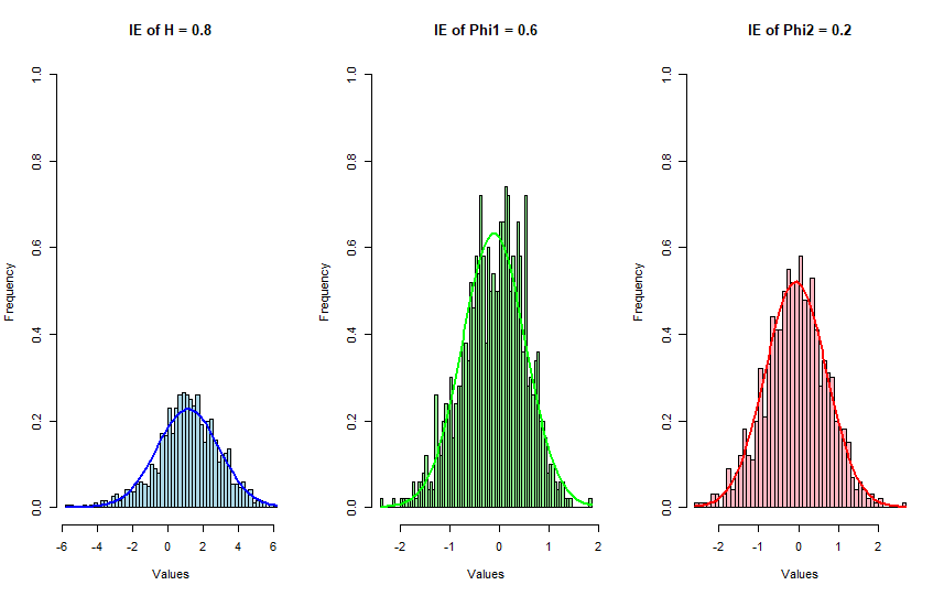
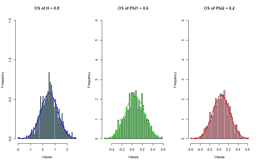
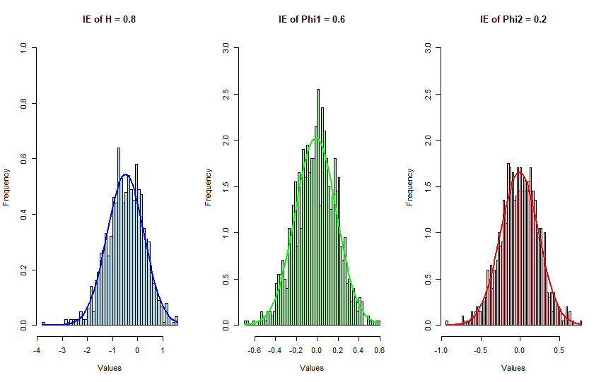
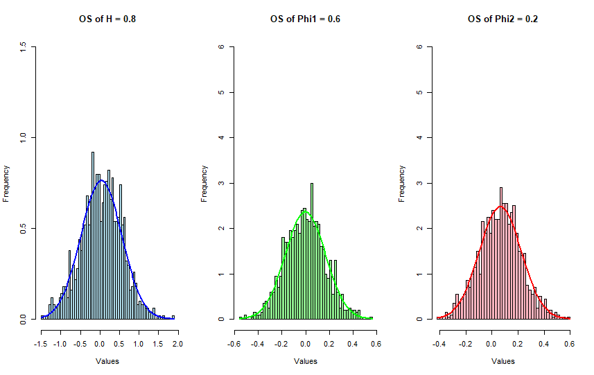
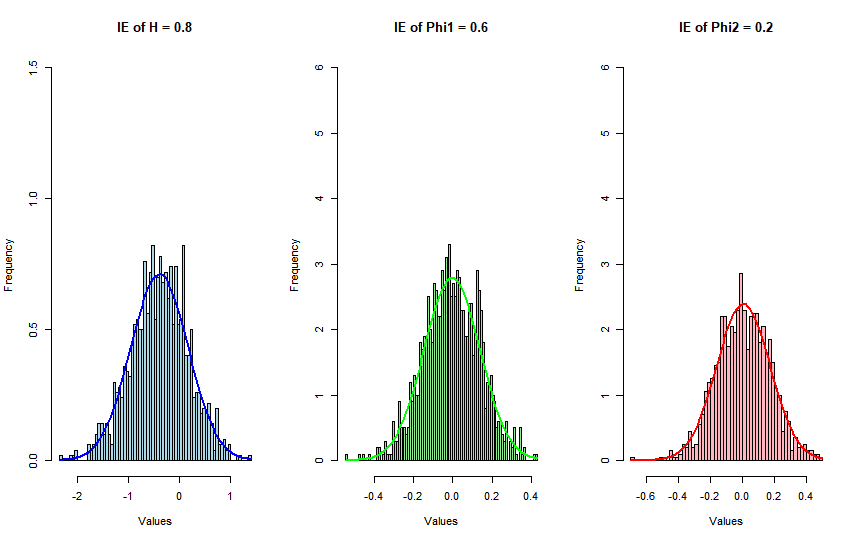
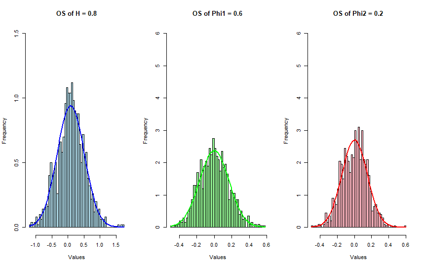
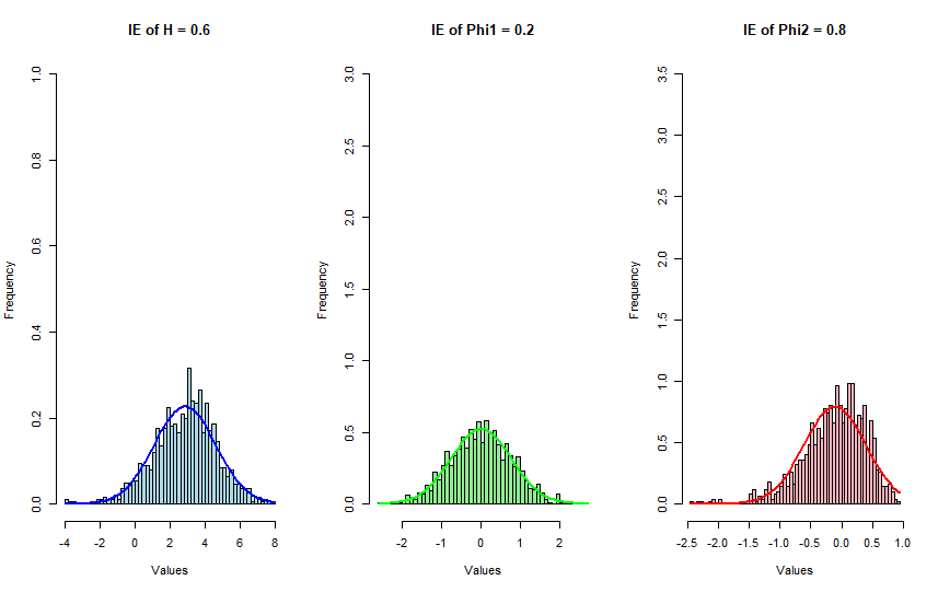
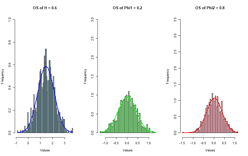
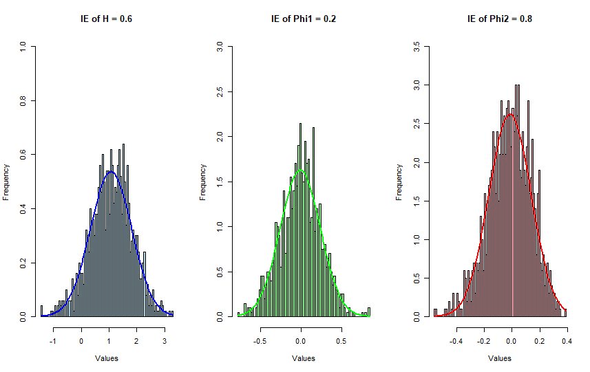
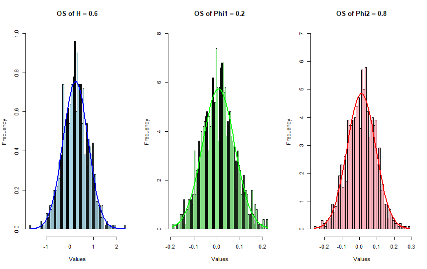
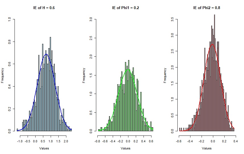
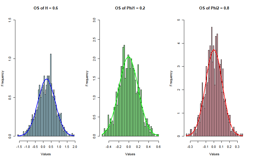
Figure 1 ,2 and 3 depict the frequency distribution of statistical errors for the initial estimatior and one-step estimatior of the SFAR(1) model with parameters , , and . Figure 4 ,5 and 6 depict the frequency distribution of statistical errors for the initial estimatior and one-step estimatior of the SFAR(1) model with parameters , , and .
In all the tables, B stands for Bias, IE represents initial estimator, and OS denotes one-step estimator. From the above tables, it can be seen that the OS estimator shows a significant improvement in the estimation of . From these figures and the accompanying table, it is evident that the one-step estimatior outperforms the initial estimation, with a particularly notable improvement in estimating the parameter , at the same time, we found that as the sample size increases, the estimation becomes more efficient. According to Hariz et al. (2024) and our simulations, the one-step estimation also has a faster running speed.
5 Conclusions and perspectives
In this paper, we propose a simple and effective method for estimating the parameters of the SFAR model individually, and we derive the asymptotic properties of this method. We address the difficulty of parameter estimation caused by the non-stationarity of the model by creating new subseries and obtaining an explicit form for the spectral density of the additive series.
The one-step procedure is essentially a gradient descent approach, achieving the rate with optimal variance.
Our results can be extended to SARIMA models by adjusting the calculation of the covariance matrix of the noise and the spectral density of . Additionally, more effective initial estimators can be utilized for the one-step procedure, similar to the approach taken by Hariz et al. (2024) in the estimation of FARIMA models.
An interesting aspect to consider is that when is sufficiently large, even larger than , but still finite, the effectiveness of this gradient descent approach may diminish. In such cases, alternative methods for optimizing the initial estimator should be explored.
6 Application on Real Data
In this section, we will conduct practical modeling and analysis to examine the application effectiveness of the seasonal autoregressive model driven by fractional Gaussian noise in real data.
The data on the Colorado River runoff in Arizona selected in this paper are from the public data of the United States Geological Survey. This dataset records the monthly river runoff of the Colorado River from 1922 to 2022, with the unit of cubic feet per second. To facilitate modeling, we average the data of each of the 12 months on a quarterly basis, obtaining the quarterly runoff data for the first, second, third, and fourth quarters respectively. First, we calculate and obtain the autocorrelation function (ACF) plot and partial autocorrelation function (PACF) plot of the quarterly runoff data as follows:
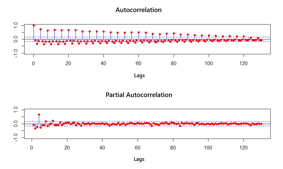
From the above figure, we can observe that the autocorrelation function shows a trailing pattern with a slow decay rate, while the partial autocorrelation function cuts off. Therefore, it is appropriate to consider using a fractional AR model with long memory properties.
To avoid data over crowding and considering that the river runoff around 1963 changed significantly for unknown reasons, we extract the runoff data from 1922 to 1962 and draw the following sample path plot.
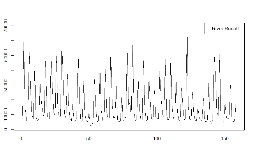
As can be seen from Figure 8, the runoff of this river exhibits obvious seasonality. Considering the above two points, in this empirical analysis, we consider using the SFAR(1) model to simulate the above observations and compare it with the simulation of the seasonal autoregressive model driven by white noise.
The seasonal autoregressive model driven by white noise is as follows:
| (43) |
where is white noise, and , , , are the model coefficients, satisfying .
We utilized the data from 1922 to 1962 to derive the parameter estimations of the two models. Subsequently, we computed their RMSEb and MAE against the real data. Finally, we randomly simulated 20 data points within these forty years using these two models. The results are shown in the following table and figure.
| Model | SFAR | SAR |
|---|---|---|
| Parameters | (, , , , ) | (, , , ) |
| Values | (0.96, 0.82, 0.80, 0.90, 0.60) | (0.80, 0.61, 0.16, 0.53) |
| RMSE | 9439.37 | 16773.58 |
| MAE | 6107.16 | 12264.90 |
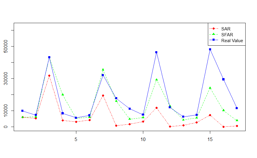
In the above figure, the values represents the parameters fitted by the SFAR and SAR model. From Figure 9 and Table 1, we can see that the seasonal autoregressive model driven by fractional noise has smaller RMSE and MAE values and better fitting performance. Therefore, the seasonal autoregressive model with long memory properties is more suitable for the study of the Colorado River runoff.
7 Proofs of the main results
For clarity, we divide the technical results into two parts. The first part addresses the stationarity and spectral density of the SFAR(1) model, as well as the asymptotic properties of the initial estimator. The second part focuses on the asymptotic properties related to the one-step estimator.
7.1 Proof of Proposition 2.1
We will utilize the following lemma to demonstrate the stationarity of .
Lemma 7.1.
For any , the SFAR(1) model is defined by the recursive scheme
| (44) |
where is a fractional Gaussian noise, , , then is a stationary process.
Proof.
We verify that the process satisfies the three conditions for weak stationarity individually.
(1) For any , is a finite constant.
Because the equation has a root outside the unit circle, the process is said to be an SFAR(1) process if it can be represented as follows
| (45) |
without loss of generality, we assume . For any time series under the monotone convergence theorem and the Cauchy-Schwarz inequality, we obtain
We know that as for . Consequently, is absolutely summable, i.e., . Thus, as shown in equation (7.1). By the monotone convergence theorem, is absolutely convergent almost surely.
Considering that
| (47) |
with the dominated convergence theorem,
| (48) |
(2) For any , .
From equation (45), we derive
by applying the conclusion above, we obtain
| (50) |
and the covariance of and is
| (51) |
Since is absolutely summable, it is also square summable. Additionally, as , , implying that there exists a constant such that . Based on the above discussion and equation (7.1), we have established that .
(3) For any , , which means that the autocovariance of and depends only on the time interval .
Without losing of generality, we assume and the covariance of be rewritten as
| (52) | ||||
for any , it follows directly from the above equation that
| (53) |
Thus, we have shown that is stationary. Since is a combination of in a cyclic manner, its stationarity naturally follows. ∎
7.2 Proof of Proposition 2.2
Since the stationarity of has been established, we can determine its spectral density using Theorem 4.4 (Brockwell & Davis, 1991). satisfies the recursion
From the above expression, we obtain the transfer function as follows
| (55) |
Thus, the spectral density function is given by
| (56) |
7.3 Proof of Proposition 2.3
Because the stationarlity of has been proved above, has the following expression
and the coefficient of transfer function has the form of
| (58) |
Then the transfer function is given by
| (59) |
To simplify the notation, we denote
| (60) |
Then, we have
| (61) |
and the spectral density of has the representation
| (62) |
Remark 10.
denote the modulus of .
7.4 Proof of Theorem 2.4
The first part of the proof to to establish the consistency of , while second part is to verify consistency of .
(1) Consistency of
This proof is based on Lemma 5.5 (Hariz et al., 2024) and the corollary (Hurvich et al., 1998). We can express in the following form
According to Hurvich et al. (1998), it can be concluded that
| (64) |
where is the error defined in Equation (3) of Hurvich et al. (1998). According to the theorem 1 from the aforementioned sources, we have
| (65) |
Hence, it is evident that
| (66) |
(2) Consistency of
Assuming
| (67) |
we can derive the following expression
| (68) |
We apply the taylor expansion of the matrix at to the the numerator, yielding
| (69) | ||||
thanks to the work of Hariz et al. (2024), we have the following three conclusions
| (70) |
| (71) |
| (72) |
where , are constants, , and , , are
| (73) |
| (74) | ||||
| (75) | ||||
It has been demonstrated in Esstafa (2019) that
| (76) |
the combination of equations (70), (71), (72), and (76) allows us to deduce that
| (77) |
Next, we consider the asymptotic properties of the denominator of equation (68). We can similarly expand the denominator using a Taylor series around , resulting in
| (78) | ||||
similarly, this part of the proof aligns with Lemma 1 (Esstafa, 2019) and satisfy
| (79) |
| (80) |
| (81) |
where is a constant. The denominator in equation (68) converges in probability as follows
| (82) |
Combining the above equations, we find that when the numerator of equation (68) is multiplied by , it approaches , while the denominator, also multiplied by , converges to a constant. Furthermore, since convergence in probability implies convergence in distribution, we conclude that
| (83) |
This establishes a clear relationship between the asymptotic behavior of the numerator and denominator, leading to the convergence of the estimated function.
7.5 Proof of Theorem 2.5
According to Theorem 2 (Hurvich et al., 1998), without loss of generality, we can assume for some . denotes convergence in distribution. We thus have
| (84) |
where is a constant related to and . Building on the results from equation (68), we establish that
| (85) |
according to the proof of consistency and some results on Esstafa (2019),the denominator of the first term on the right side of the above equation satisfies
| (86) |
the nominator converge to a normal distribution
| (87) |
when , the reminder converges to 0.
Thus, we can rewrite equation (85) as follows
by slutsky theorem, we can conclude that converges to a normal distribution.
Lastly, we aim to present these results in the form of a joint normal distribution. Drawing on the findings from Hariz et al. (2024), the asymptotic distribution of can be expressed as a constant multiple of the asymptotic distribution of . Moreover, according to the Cramer-Wold theorem, the asymptotic distribution of still adheres to an asymptotic normal distribution. Thus, the vector
converges to a Gaussian vector, tending towards a joint normal distribution. The covariance matrix of this vector is
| (89) |
where
| (90) |
is the constants related to and .
7.6 Proof of Theorem 3.1
To prove the theorem 3.1, we need to establish the following three lemmas and verify whether is regular. The regularity conditions of will be demonstrated in the auxiliary results.
Lemma 7.2.
Let , , such that for any , it holds that
| (91) |
where is some constant.
Proof.
Without loss of generality, let be a convex set in . For ease of notation, can be denoted as . According to the relevant conclusions in Cohen et al. (2011) and the discussion of regularity conditions for , it is known that for any that the following inequality holds
| (92) |
is defined as
| (93) |
which is related to and . Furthermore, since the conditions (A1) and (A2) (Cohen et al., 2011) hold, it follows that , hence the lemma holds. ∎
Lemma 7.3.
For any , it follows from the distribution of the parameter that
| (94) |
Proof.
The Lemma 3.6 (Cohen et al., 2011) implies that, from the distribution of , we have
| (95) |
To determine the convergence rate of the above expression, Lemma 3 and Lemma 4 (Lieberman et al., 2012) yield the following conclusion
| (96) |
where is a positive real number. Therefore,
| (97) |
Furthermore, by utilizing Lemma 3.6 (Cohen et al., 2011) once again, we obtain
| (98) |
Thus, the proof is concluded. ∎
Lemma 7.4.
Let be a stochastic sequence satisfying . Then, according to the distribution of parameter , for any , it holds that
| (99) |
Proof.
Let be a compact convex set depending on and , and . According to the proof of Lemma 3.7 (Cohen et al., 2011), we have
| (100) |
where , satisfying . In conclusion, for a finite positive random variable , we have
| (101) |
which implies holds. ∎
According to the hypothesis of this theorem, we can deduce
| (102) |
applying mean-value theorem to , we have
| (103) |
Substituting equation (103) to equation (102), we produce
| (104) |
where = , .
Next, we will discuss the consistency and asymptotic normality of one-step estimator.
(1) Consistency of
Observing equation (104) , the first and second terms on the right-hand side can be expressed as
and
| (106) |
Fristly, we analyze the properties of and derive the following equation
| (107) | ||||
based on equation (107) and lemmas 6.2, 6.3, and 6.4. The convergence order of is
| (108) |
when , we have .
Secondly, we consider the property of and it has the form of
| (109) |
according to Hariz et al. (2024) and theorem 1 in Lieberman et al. (2012), we have
| (110) |
When is a non-degenerate continuous function, as indicated by the above equation, it can be observed that both the first and second terms of tend to 0. Consequently, converges in probability to 0, and naturally, it also converges in distribution to 0.
Combining the above results, we can conclude the consistency of .
(2) Asymptotic normality of
8 Auxiliary results
Lemma 8.1.
Under the hypothesis on the parametric space have the following results
(1) For any and , .
(2) For any the functions are symmetric with respect to .
(3) For any and all
a.
b.
c.For any ,
where are constants for
Proof.
We start from Assertion 3a, which states that
| (112) |
where and denote the Gamma function. According to Lemma 5.4 in Hariz et al. (2024), we have
| (113) |
and
| (114) |
where and are the maximum and minimum values of , respectively. Thus, Assertion 3a has been proved and assertion 3b follows straightforwardly from Assertion 3a.
Next, we discuss Assertion 3c, which can be obtained directly from Lemma 5.4 in Hariz et al. (2024). The partial derivative of does not depend on , and the modulus is bounded.
∎
References
- Beran et al. (2013) Beran, J., Feng, Y., Ghosh, S., & Kulik, R. (2013). Long-memory processes. Long-Mem. Process. https://doi.org/10.1007/978-3-642-35512-7
-
Bisognin & Lopes (2009)
Bisognin, C., & Lopes, S. R. C. (2009). Properties of seasonal long memory processes. Mathematical and Computer Modelling, 49(9-10), 1837-1851. https://doi.org/10.1016/j.mcm.200
8.12.003 - Brockwell & Davis (1991) Brockwell, P. J., & Davis, R. A. (1991). Time series: theory and methods. Springer Science & Business Media. https://doi.org/10.2307/2982983
- Brouste et al. (2014) Brouste, A., Cai, C., & Kleptsyna, M. (2014). Asymptotic properties of the MLE for the autoregressive process coefficients under stationary Gaussian noise. Mathematical Methods of Statistics, 23, 103-115. https://doi.org/10.3103/S1066530714020021
- Brouste et al. (2020) Brouste, A., Soltane, M., & Votsi, I. (2020). One-step estimation for the fractional Gaussian noise at high-frequency. ESAIM: Probability and Statistics. https://doi.org/10.1007/978-3
- Carlin & Dempster (1989) Carlin, J. B., & Dempster, A. P. (1989). Sensitivity analysis of seasonal adjustments: empirical case studies. Journal of the American Statistical Association, 84(405), 6-20. https://doi.org/10.2307/2289837
- Chan & Terrin (1995) Chan, N. H., & Terrin, N. (1995). Inference for unstable long-memory processes with applications to fractional unit root autoregressions. The Annals of Statistics, 23(5), 1662-1683. https://doi.org/10.1214/aos/1176324318
- Chatfield & Prothero (1973) Chatfield, C., & Prothero, D. L. (1973). Box‐Jenkins seasonal forecasting: problems in a case‐study. Journal of the Royal Statistical Society: Series A (General), 136(3), 295-315. https://doi.org/10.2307/2344994
- Cohen et al. (2011) Cohen, S., Gamboa, F., Lacaux, C., & Loubes, J. M. (2011). LAN property for some fractional type Brownian motion. ALEA: Latin American Journal of Probability and Mathematical Statistics, 10(1), 91-106.
- Esstafa (2019) Esstafa, Y. (2019). Long-memory time series models with dependent innovations (Doctoral dissertation, Université Bourgogne Franche-Comté).
- Fox & Taqqu (1986) Fox, R., & Taqqu, M. S. (1986). Large-sample properties of parameter estimates for strongly dependent stationary Gaussian time series. The Annals of Statistics, 14(2), 517-532. https://doi.org/10.1214/aos/1176349936
- Franco & Reisen (2007) Franco, G. C., & Reisen, V. A. (2007). Bootstrap approaches and confidence intervals for stationary and non-stationary long-range dependence processes. Physica A: Statistical Mechanics and its Applications, 375(2), 546-562. https://doi.org/10.1016/j.physa.2006.08.027
- Geweke & Porter‐Hudak (1983) Geweke, J., & Porter‐Hudak, S. (1983). The estimation and application of long memory time series models. Journal of Time Series Analysis, 4(4), 221-238. https://doi.org/10.1111/j.1467-9892.1983.tb00371.x
- Gloter & Yoshida (2021) Gloter, A., & Yoshida, N. (2021). Adaptive estimation for degenerate diffusion processes. https://doi.org/10.1214/20-EJS1777
- Hariz et al. (2024) Hariz, S.B., Brouste, A., Cai, C., & Soltane, M. (2024). Fast and asymptotically-efficient estimation in an autoregressive process with fractional type noise. Journal of Statistical Planning and Inference. https://doi.org/10.1016/j.jspi.2024.106148
- Harrison (1965) Harrison, P. J. (1965). Short‐term sales forecasting. Journal of the Royal Statistical Society: Series C (Applied Statistics), 14(2-3), 102-139. https://doi.org/10.1287/mnsc.13.11.821
-
Hosking (1984)
Hosking, J. R. (1984). Modeling persistence in hydrological time series using fractional differencing. Water Resources Research, 20(12), 1898-1908. https://doi.org/10.1029/WR020i012
p01898 - Hurst (1951) Hurst, H. E. (1951). Long-term storage capacity of reservoirs. Transactions of the American Society of Civil Engineers, 116(1), 770–799. https://doi.org/10.1061/TACEAT.0006518
- Hurvich et al. (1998) Hurvich, C. M., Deo, R., & Brodsky, J. (1998). The mean squared error of Geweke and Porter‐Hudak’s estimator of the memory parameter of a long‐memory time series. Journal of Time Series Analysis, 19(1), 19-46. https://doi.org/10.1111/1467-9892.00075
- Kong & Lund (2023) Kong, J., & Lund, R. (2023). Seasonal count time series. Journal of Time Series Analysis, 44(1), 93-124. doi:10.1111/jtsa.12651
- Kutoyants & Motrunich (2016) Kutoyants, Y. A., & Motrunich, A. (2016). On multi-step MLE-process for Markov sequences. Metrika, 79, 705-724. https://doi.org/10.1007/s00184-015-0574-4
- Le Cam (1956) Le Cam, L. (1956). On the asymptotic theory of estimation and testing hypotheses. In Proceedings of the Third Berkeley Symposium on Mathematical Statistics and Probability, Volume 1: Contributions to the Theory of Statistics (Vol. 3, pp. 129-157). University of California Press. https://doi.org/10.1525/9780520313880-014
- Lieberman et al. (2012) Lieberman, O., Rosemarin, R., & Rousseau, J. (2012). Asymptotic theory for maximum likelihood estimation of the memory parameter in stationary Gaussian processes. Econometric Theory, 28(2), 457-470. https://doi.org/10.1017/S0266466611000399
- Marinucci & Robinson (1998) Marinucci, D., & Robinson, P. M. (1998). Semiparametric frequency domain analysis of fractional cointegration. https://doi.org/10.1093/oso/9780199257294.003.0015
- Robinson (1995) Robinson, P. M. (1995). Log-periodogram regression of time series with long range dependence. The Annals of Statistics, 1048-1072. https://doi.org/10.1214/aos/1176324636
-
Robinson (2010)
Robinson, P. M. (2010). Long memory models. In Macroeconometrics and Time Series Analysis (pp. 163-168). London: Palgrave Macmillan UK. https://doi.org/10.1093/acrefore/97801906
25979.013.173 - Soltane (2024) Soltane, M. (2024).Asymptotic efficiency in autoregressive processes driven by stationary Gaussian noise. Stochastic Models, 40(1), 70–96.https://doi.org/10.1080/15326349.2023.2202227
- Tsay (2013) Tsay, R. S. (2013). Multivariate time series analysis: with R and financial applications. John Wiley & Sons.