Theory of the correlated quantum Zeno effect in a monitored qubit dimer
Abstract
We theoretically investigate the stochastic dynamics of two qubits subject to one- and two-site correlated continuous weak measurements. When measurements dominate over the local unitary evolution, the system’s dynamics is constrained and part of the physical Hilbert space becomes inaccessible: a typical signature of the Quantum Zeno (QZ) effect. In this work, we show how the competition between these two measurement processes give rise to two distinct QZ regimes, we dubbed standard and correlated, characterised by a different topology of the allowed region of the physical Hilbert space being a simply and non-simply connected domain, respectively. We develop a theory based on a stochastic Gutzwiller ansatz for the wavefunction that is able to capture the structure of the phase diagram. Finally we show how the two QZ regimes are intimately connected to the topology of the flow of the underlying non-Hermitian Hamiltonian governing the no-click evolution.
Introduction – A watched pot never boils over, or does it? According to quantum mechanics, it depends on the rate at which we watch the pot. In a generic quantum system, the unitary evolution, which tends to delocalize the wavefunction over the entire Hilbert space, competes with quantum measurements, which, on the contrary, hamper the system’s dynamics [1]. When measurements dominate over the Hamiltonian dynamics, the wavefunction gets localized in a specific region of the Hilbert space, giving rise to the celebrated QZ effect [2, 3, 4, 5, 6, 7, 8, 9].
The accurate monitoring of quantum fluctuations of the measuring apparatus leads to the possibility of tracking individual quantum trajectories, i.e. to resolve single instances of the stochastic evolution of the system’s wavefunction [10, 11, 12, 13, 14]. By collecting many trajectories one can construct the statistical mixture of states explored by the system, i.e. the system density matrix. While the same mixture can be constructed in many different ways, a fact known as ensemble ambiguity [15, 16], the knowledge of its unravelling in terms of trajectories gives much more informations about the underlying monitored dynamics, including space-time correlations and the full counting statistics of the observables [17, 18, 19].
At a given time the statistics of the trajectories can be condensed in the probability density function (PDF) that provides the probability to find the quantum state in a specific position of the Hilbert space. For a single qubit, the structure of the PDF provides a direct proxy for the emergence of the QZ effect featuring forbidden regions where at long times the PDF vanishes [20]. When more than one body is considered, interactions play a crucial role in determining the onset of the QZ effect [21, 22, 23, 24, 25, 26, 27, 28, 29]. Furthermore, on a lattice, correlated multi-site measurements (i.e. the detection of the collective state of the sites involved) are possible and compete with one-site monitoring [30, 31]. In the latter case, the structure of the PDF is generally unknown, and the impact of different detection schemes and measurements remains unexplored.
(a)
(b)
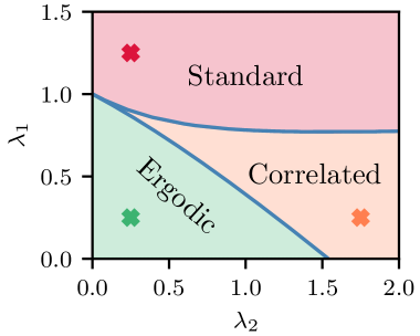
To address these fundamental questions, this study explores a minimal model composed of two qubits subject to one- and two-qubit measurements and undergoing local unitary dynamics. We show that the competition between the two kinds of measurements and Hamiltonian evolution leads to the emergence of two distinct QZ regimes characterized by a different topology of the PDF. Our main result is that simultaneous two-qubit measurements stabilize a correlated QZ regime where the topology of the PDF is a non-simply connected domain surrounding a non-accessible region. On a physical ground, this result establishes that each qubit can be found in any possible state, i.e. it fully spreads over its local Hilbert space, but some configurations of the two qubits are forbidden. Extending the famous proverb we claim that two pots watched simultaneously never boil together, however they do it separately.
When one-qubit measurements dominate over the correlated ones, the dynamics of the two qubits effectively decouples, and the system approaches a standard QZ regime where only a simply connected domain of the physical Hilbert space is explored during the dynamics. We determine the boundaries of the different phases in the parameter space, developing a theory based on the stochastic Gutzwiller ansatz for the dimer wavefunction [32, 33, 34, 35]. The phase diagram of the model is shown in Fig.1. We also show that the different topology of the PDF is in one-to-one correspondence with the topology of the flow [36] of the postselected non-Hermitian no-click evolution.
Model and measurement protocol – We consider two identical two-level systems each performing coherent oscillations between the states and ( and refer to the left and right spin, respectively) due to the Hamiltonian , where is the oscillation frequency (hereafter we set ). The two qubits also be monitored by a sequence of variable strength measurements at an interval .
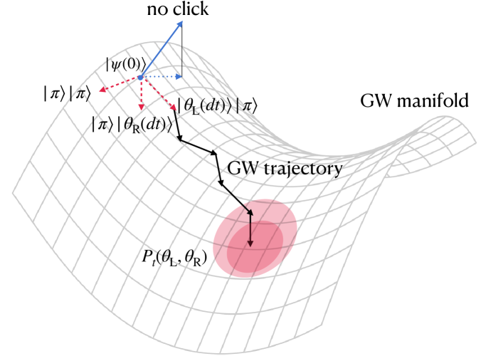
By coupling the system with ancillary qubits appropriately, it is possible to construct a protocol where both the on-site populations and the two-qubit density correlations are measured. A sketch of the setup under consideration is shown in Fig. 1 (see also [37] for details of the physical model). More formally, each measurement event is characterised by four possible readouts , which give rise to the following back-actions on the system
| (1) |
where , and control the measurement strength. Readouts account for on-site measurement of the and qubit population, respectively. The readout accounts for the correlated measurement of the two qubits. Finally, the event where none of the detectors click, , often referred in the literature as no-click event. We are interested in the regime where with and . According to the Born rule, the probability of obtaining each of the readouts on a state is given by for [15].
In each time step the unitary dynamics and measurement combine into the evolution
| (2) |
where and ensures the normalization of the post-measurement state.
Note that in the monitoring protocol we are considering, the two qubits do not interact because of the unitary evolution, but they are coupled via the readouts and of the measurement procedure. When , the no-click dynamics can be written in terms of a non-Hermitian Hamiltonian. Indeed where
| (3) |
The last term in Eq. (3) explicitly couples the two qubits and generates entanglement among them. When , we know that after the measurement the two-qubit state will coincide with the pointer state , thus completely correlating (classically) the states of the two qubits.
The stochastic Gutzwiller ansatz – In order to get further insights about the monitored dynamics, we propose a Gutzwiller ansatz that for the dimer under investigation takes the form
| (4) |
The ansatz (4) allows to capture the build up of classical correlations between the left and right qubit induced by the monitoring dynamics and will neglect the quantum ones due to the fact that the state is always factorisable. This approximation is well justified in our problem since clicks (, see Eq. (1)) collapse the system to factorised states. It is therefore reasonable to assume that the system will remain in the vicinity of a factorised state at all times. Only the no-click event () couples the two qubits, generating both classical and quantum correlation. The extent to which this approximation is justified quantitatively will be evaluated by comparing the approximate results to simulations of the full system dynamics for the quantities of interests.
Very conveniently, in the Gutzwiller approximation the state of the system can be represented on two Bloch spheres, one for each qubit. In fact, for a suitable set of initial states such that , the dynamics of the system is confined to a section of the two spheres. Hence, one angle for each qubit is sufficient for describing the state that can be parametrized as . Thus, the pair of variables fully determine the state of the dimer.
Within the Gutzwiller approximation, the dynamics of the system can then be rewritten as a time evolution of the two variables and . In terms of these Eq. (2) becomes (see [37] for the details of the derivation):
| (5) |
where and , with the effective adimensional measurement strengths . Equation (5), complemented with the readout probabilities in the Gutzwiller approximation
| (6) |
describes a stochastic evolution of the two variables and pictorially represented in Fig.2. Summarizing: measurements yielding readouts project the L (R) qubit onto the state (). Measurements yielding the readout take the system to the state . While when the readout (no-click) is obtained the variables evolve infinitesimally with velocity .
Finally, we stress that this approach can be easily extended to the -qubit scenario. In such case, this would translate into a set of non-linear stochastic equations for the angles fully parametrizing the state.
Probability density of the quantum state – The main quantity we are interested in is the PDF that represents the probability for the system of being in the state at time given the ensemble of trajectories generated by the monitored dynamics. In general, for a system of spins, this is a function of the parameters that are needed to pinpoint a state in the system’s Hilbert space. However, within the Gutzwiller framework, the state of the dimer is fully determined by the variables . Operationally, this function can be written as
| (7) |
where is the state at time along the -th trajectory, , and is the number of trajectories. This PDF directly probes the states’ spreading in the portion of the Hilbert space explored by the dynamics. It is thus a powerful tool to witness the onset the QZ effect, which hampers the state evolution creating forbidden regions in said portion of the Hilbert space. The master equation governing the dynamics of is derived in [37].
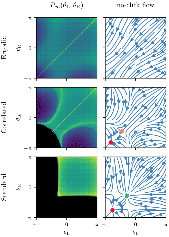
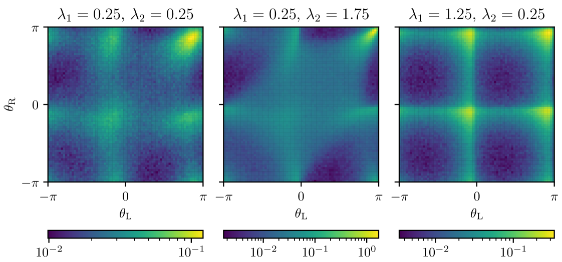
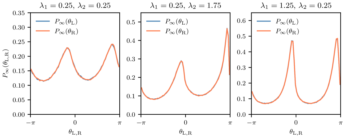
The left panels in Fig.3 show a Monte Carlo solution of the stationary distribution for a selection of measurement strengths, and . The three plots represent three different qualitative behaviours of the system. The transitions between these regimes are sharp and define a phase diagram for the dimersummarized in Fig. 1. For small coupling values, the system is in an ergodic phase, where the measurement strengths are too weak to create forbidden regions. As a result the whole Hilbert space can be populated at long times. At larger values of and small enough the system enters a correlated QZ phase where a forbidden region of angles pairs appears close to . However and can still assume all values individually. In other words, a single spin can be found everywhere on its Bloch sphere, but some combinations of the two angles are forbidden. This is a consequence of the structure of the two-qubit measurement operator that acts more and more effectively as both spins are close to . Finally, when is increased, regardless of the value of , the system enters a standard Zeno phase where entire intervals of and are never reached by the dynamics. We also note that given the symmetry of the unitary and measurement processes, we have .
From Fig. 3 it is clear that the correlated and the standard Zeno regions feature a different topology of the PDF describing the Hilbert space explored by the stochastic evolution. In the correlated Zeno region, upon mapping on a torus, the allowed portion of the Hilbert space becomes a non-simply connected domain surrounding a non-accessible region. In the standard Zeno region, local measurements dominates over the correlated ones. The system approaches the standard QZ regime where only a simply connected domain of the physical Hilbert space is explored during the dynamics. In the latter case, we observe that
| (8) |
reflecting the fact that strong local monitoring decouples the dynamics of the two qubits. In Eq.(8) the equality holds exactly when . We conclude by noticing that the structure of the PDF in the correlated Zeno region is a direct consequence of the correlation between the two qubits, which implies .
No-click dynamics – The three distinct behaviours exhibited by the PDF presented above can be understood by studying the no-click evolution of the model given by the part of Eq. (5). Upon this post-selection, the dynamics is deterministic and described by the non-Hermitian evolution of the variables as follows
| (9) |
The right panels of Fig. 3 show the flow determined by the differential equation (9) for a selection of values of measurement strengths and 111The flow represents the 2D velocity field of the variables under the no-click dynamics of Eq. (9). The velocity (tangent to the streamlines) at any point is given by . In the figure the flow should be thought of as periodic: flow-lines that exit at the bottom and left re-enter from the top and right respectively. The flow exhibits three qualitatively different behaviours in correspondence of the regions identified previously. In the ergodic region, the flow has no fixed points. In the correlated Zeno region the flow develops two fixed points along the diagonal . One of the two points is unstable (red dot), while the other is a saddle (orange dot). In the standard Zeno region, the flow develops four fixed points, two of which are again on the diagonal. Of these two, one is still an unstable point (red dot), while the second is stable (green dot).
The appearance of dynamically forbidden states can be understood from the no-click flow by considering how clicks combine with it. From a generic point , clicks can take the system to one of , , or , that is to the right edge, top edge, or right-top corner of the plots, respectively. In the limit that we are considering, all trajectories eventually click, independently of the initial conditions. Without loss of generality, we can thus focus on trajectories with starting points on the top or right edges of the figure. By inspecting the no-click flow in the right panels of Fig. 3, we can then conclude that in the ergodic region all states are reachable. In the correlated Zeno region, there is a region close to the bottom-left corner that cannot be reached by trajectories that have their starting point on the top and right edges; In standard Zeno region then entire intervals of and are eventually depleted by clicks that take the system to the state .
Summarizing, the three distinct regimes of the two-qubit system under varying measurement strengths and are in one-to-one correspondence with the structure of the flow of the no-click evolution. The boundaries between the different regimes depicted in Fig. 1 can be thus obtained by studying the structure of the PDF or, equivalently, computing the fixed points of the flow under the non-Hermitian evolution. Notably, the topologically distinct regimes are a key feature of the quantum jump dynamics. Different measurement schemes, such as Quantum State Diffusion, would lead to the disappearance of the forbidden region, as shown in Appendix .2, which is the case for a single qubit dynamics as well.
Comparison with full dynamics– The main difference between the Gutzwiller and full dynamics is that the former is not able to capture quantum entanglement between the two qubits. The disagreement between the results is a measure of the relevance of quantum correlations in the dynamics of the system.
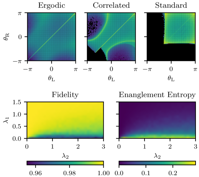
The top panels in Fig. 4 show that the stationary PDF for the two angles, and , computed by simulating the full dynamics of the system, exhibit the same qualitative behaviour, with three distinct regimes as described previously in the Gutzwiller approximation 222Given that the full wavefunction is in general not factorizable one has to compute the on-site reduced density matrix for the qubit and exploit the Bloch sphere representation which gives directly access to and thus compute the PDF.. In order to get further insights about the accuracy of the approximation in the different regimes we computed fidelity between the exact trajectories and the Gutzwiller ones and the entanglement entropy of the former, respectively
| (10) |
where is the exact state along the -th trajectory, is the corresponding reduced density matrix of the L qubit and is its closest Gutzwiller state.
Unsurprisingly, the quantitative differences that can be observed between the full and Gutzwiller PDFs are greater at high values of the ratio. This can be explained by observing that the only entangling coupling between the two qubits is given by the two-body measurement part of the non-Hermitian Hamiltonian (3), whose strength is set by . Interestingly, also at large values of , moderate values of are sufficient to strongly suppress quantum entanglement of the trajectories.
Conclusions – In this work, we have proposed a theory to explain the emergence of the QZ effect in a monitored qubit dimer. Our analysis has led to the identification of two qualitatively distinct QZ regimes, each characterized by a different topology in the probability density function (PDF). This behavior was further linked to the underlying topology of the no-click flow in the system.
Building on these foundational results, our theory can be extended to many-body spin systems. A promising direction for future research would be the exploration of how the topology of allowed and forbidden regions varies as a function of different multi-site measurement protocols via the generalization of the stochastic Gutzwiller ansatz.
Acknowledgements – We thank Rosario Fazio, Marcello Dalmonte, Philipp Hauke, Alessandro Roggero and Oded Zilberberg for inspiring discussions. AB acknowledges financial support from the Provincia Autonoma di Trento and by the European Union — NextGeneration EU, within PRIN 2022, PNRR M4C2, Project TANQU 2022FLSPAJ [CUP B53D23005130006]. AR and GC acknowledge support by EPSRC via Grant No. EP/W524438/1.
References
- Breuer and Petruccione [2002] H. P. Breuer and F. Petruccione, The theory of open quantum systems (Oxford University Press, Great Clarendon Street, 2002).
- Misra and Sudarshan [1977] B. Misra and E. C. G. Sudarshan, The zeno’s paradox in quantum theory, Journal of Mathematical Physics 18, 756 (1977), https://doi.org/10.1063/1.523304 .
- Peres [1980] A. Peres, Zeno paradox in quantum theory, American Journal of Physics 48, 931 (1980), https://doi.org/10.1119/1.12204 .
- Itano et al. [1990] W. M. Itano, D. J. Heinzen, J. J. Bollinger, and D. J. Wineland, Quantum zeno effect, Phys. Rev. A 41, 2295 (1990).
- Facchi et al. [2001] P. Facchi, H. Nakazato, and S. Pascazio, From the quantum zeno to the inverse quantum zeno effect, Phys. Rev. Lett. 86, 2699 (2001).
- Facchi and Pascazio [2002] P. Facchi and S. Pascazio, Quantum zeno subspaces, Phys. Rev. Lett. 89, 080401 (2002).
- Kwiat et al. [1999] P. G. Kwiat, A. G. White, J. R. Mitchell, O. Nairz, G. Weihs, H. Weinfurter, and A. Zeilinger, High-efficiency quantum interrogation measurements via the quantum zeno effect, Phys. Rev. Lett. 83, 4725 (1999).
- Wolters et al. [2013] J. Wolters, M. Strauß, R. S. Schoenfeld, and O. Benson, Quantum zeno phenomenon on a single solid-state spin, Phys. Rev. A 88, 020101 (2013).
- Signoles et al. [2014] A. Signoles, A. Facon, D. Grosso, I. Dotsenko, S. Haroche, J.-M. Raimond, M. Brune, and S. Gleyzes, Confined quantum zeno dynamics of a watched atomic arrow, Nature Physics 10, 715 (2014).
- Guerlin et al. [2007] C. Guerlin, J. Bernu, S. Deléglise, C. Sayrin, S. Gleyzes, S. Kuhr, M. Brune, J.-M. Raimond, and S. Haroche, Progressive field-state collapse and quantum non-demolition photon counting, Nature 448, 889 (2007).
- Sayrin et al. [2011] C. Sayrin, I. Dotsenko, X. Zhou, B. Peaudecerf, T. Rybarczyk, S. Gleyzes, P. Rouchon, M. Mirrahimi, H. Amini, M. Brune, J.-M. Raimond, and S. Haroche, Real-time quantum feedback prepares and stabilizes photon number states, Nature 477, 73 (2011).
- Murch et al. [2013a] K. W. Murch, S. J. Weber, K. M. Beck, E. Ginossar, and I. Siddiqi, Reduction of the radiative decay of atomic coherence in squeezed vacuum, Nature 499, 62 (2013a).
- Murch et al. [2013b] K. W. Murch, S. J. Weber, C. Macklin, and I. Siddiqi, Observing single quantum trajectories of a superconducting quantum bit, Nature 502, 211 (2013b).
- Weber et al. [2014] S. J. Weber, A. Chantasri, J. Dressel, A. N. Jordan, K. W. Murch, and I. Siddiqi, Mapping the optimal route between two quantum states, Nature 511, 570 (2014).
- Nielsen and Chuang [2011] M. A. Nielsen and I. L. Chuang, Quantum Computation and Quantum Information: 10th Anniversary Edition, 10th ed. (Cambridge University Press, USA, 2011).
- Minganti and Biella [2024] F. Minganti and A. Biella, Open quantum systems – a brief introduction (2024), arXiv:2407.16855 [quant-ph] .
- Garrahan [2018] J. P. Garrahan, Aspects of non-equilibrium in classical and quantum systems: Slow relaxation and glasses, dynamical large deviations, quantum non-ergodicity, and open quantum dynamics, Physica A: Statistical Mechanics and its Applications 504, 130 (2018), lecture Notes of the 14th International Summer School on Fundamental Problems in Statistical Physics.
- Landi et al. [2024] G. T. Landi, M. J. Kewming, M. T. Mitchison, and P. P. Potts, Current fluctuations in open quantum systems: Bridging the gap between quantum continuous measurements and full counting statistics, PRX Quantum 5, 020201 (2024).
- Fazio et al. [2025] R. Fazio, J. Keeling, L. Mazza, and M. Schirò, Many-body open quantum systems (2025), arXiv:2409.10300 [quant-ph] .
- Snizhko et al. [2020] K. Snizhko, P. Kumar, and A. Romito, Quantum zeno effect appears in stages, Phys. Rev. Research 2, 033512 (2020).
- Fröml et al. [2019] H. Fröml, A. Chiocchetta, C. Kollath, and S. Diehl, Fluctuation-induced quantum zeno effect, Phys. Rev. Lett. 122, 040402 (2019).
- Fröml et al. [2020] H. Fröml, C. Muckel, C. Kollath, A. Chiocchetta, and S. Diehl, Ultracold quantum wires with localized losses: Many-body quantum zeno effect, Phys. Rev. B 101, 144301 (2020).
- Biella and Schiró [2021] A. Biella and M. Schiró, Many-Body Quantum Zeno Effect and Measurement-Induced Subradiance Transition, Quantum 5, 528 (2021).
- Rossini et al. [2021] D. Rossini, A. Ghermaoui, M. B. Aguilera, R. Vatré, R. Bouganne, J. Beugnon, F. Gerbier, and L. Mazza, Strong correlations in lossy one-dimensional quantum gases: From the quantum zeno effect to the generalized gibbs ensemble, Phys. Rev. A 103, L060201 (2021).
- Seclì et al. [2022] M. Seclì, M. Capone, and M. Schirò, Steady-state quantum zeno effect of driven-dissipative bosons with dynamical mean-field theory, Phys. Rev. A 106, 013707 (2022).
- Rosso et al. [2022] L. Rosso, L. Mazza, and A. Biella, Eightfold way to dark states in su(3) cold gases with two-body losses, Phys. Rev. A 105, L051302 (2022).
- Rosso et al. [2023] L. Rosso, A. Biella, J. De Nardis, and L. Mazza, Dynamical theory for one-dimensional fermions with strong two-body losses: Universal non-hermitian zeno physics and spin-charge separation, Phys. Rev. A 107, 013303 (2023).
- Leung and Romito [2024] C. Y. Leung and A. Romito, Entanglement and operator correlation signatures of many-body quantum zeno phases in inefficiently monitored noisy systems (2024), arXiv:2407.11723 [quant-ph] .
- Wauters et al. [2025] M. M. Wauters, E. Ballini, A. Biella, and P. Hauke, Symmetry-protection zeno phase transition in monitored lattice gauge theories, Phys. Rev. B 111, 094315 (2025).
- Ippoliti et al. [2021] M. Ippoliti, M. J. Gullans, S. Gopalakrishnan, D. A. Huse, and V. Khemani, Entanglement phase transitions in measurement-only dynamics, Phys. Rev. X 11, 011030 (2021).
- Piccitto et al. [2023] G. Piccitto, A. Russomanno, and D. Rossini, Entanglement dynamics with string measurement operators, SciPost Phys. Core 6, 078 (2023).
- Jin et al. [2016] J. Jin, A. Biella, O. Viyuela, L. Mazza, J. Keeling, R. Fazio, and D. Rossini, Cluster mean-field approach to the steady-state phase diagram of dissipative spin systems, Phys. Rev. X 6, 031011 (2016).
- Huybrechts and Wouters [2020] D. Huybrechts and M. Wouters, Dynamical hysteresis properties of the driven-dissipative bose-hubbard model with a gutzwiller monte carlo approach, Phys. Rev. A 102, 053706 (2020).
- Verstraelen et al. [2023] W. Verstraelen, D. Huybrechts, T. Roscilde, and M. Wouters, Quantum and classical correlations in open quantum spin lattices via truncated-cumulant trajectories, PRX Quantum 4, 030304 (2023).
- Ares et al. [2024] L. Ares, J. Pinske, B. Hinrichs, M. Kolb, and J. Sperling, Restricted monte carlo wave function method and lindblad equation for identifying entangling open-quantum-system dynamics (2024), arXiv:2412.08735 [quant-ph] .
- Villa et al. [2024] G. Villa, J. del Pino, V. Dumont, G. Rastelli, M. Michałek, A. Eichler, and O. Zilberberg, Topological classification of driven-dissipative nonlinear systems (2024), arXiv:2406.16591 [cond-mat.mes-hall] .
- [37] See Supplemental Material at [URL will be inserted by publisher] for the details of a possible physical implementation of the protocol, a derivation of the stochastic Gutzwiller dynamics, and… .
- Note [1] The flow represents the 2D velocity field of the variables under the no-click dynamics of Eq. (9). The velocity (tangent to the streamlines) at any point is given by .
- Note [2] Given that the full wavefunction is in general not factorizable one has to compute the on-site reduced density matrix for the qubit and exploit the Bloch sphere representation which gives directly access to and thus compute the PDF.
- Jacobs [2014] K. Jacobs, Quantum measurement theory and its applications (Cambridge University Press, 2014).
Supplemental material
.1 Measurement protocol and its physical model
The system considered in this work is composed of two qubits, referred to as left () and right qubit (). Their evolution is the combined result of the unitary evolution under the non-interacting Hamiltonian
| (11) |
where , and continuous monitoring via a generalised measurement that is performed on them at time intervals . This protocol is represented schematically in figure 1.
The measurement that we consider has four possible outcomes, labelled . Outcomes and account for local weak measurements of the and qubit populations respectively. The corresponding back-actions on the system is given by the Kraus operators
| (12) |
where and controls the local measurement strength (which is the same for both qubits). The outcome accounts for the joint measurement of the and qubit populations. Its back-action is
| (13) |
where controls the two-body measurement strength. Finally, the outcome back-action is
| (14) |
In the literature, and for reasons that will become clear in what follows, the outcome is referred to as “no-click” while the outcomes are all referred to as “clicks”.
As usual, the probability of each of the outcomes is given by
| (15) |
for .
A physical model of the measurement consists of three auxiliary qubits, , and , that interact with the two qubits comprising the dimer. The three detector qubits are coupled to the dimer via the following Hamiltonians
| (16) |
The measurement procedure is repeated at short time intervals . At the beginning of each time interval, the three auxiliary qubits are initialised in their state, then they are left to interact coherently with the system, and are subsequently measured projectively in their basis at the end of the time interval. The initialisation and readout are assumed to last a negligible time.
Therefore, in the time interval between successive measurements, the system evolves under the total Hamiltonian given by the sum of the system’s plus the interaction with the detectors
| (17) |
While the effect of the measurement on the system is obtained by computing the following back-actions
| (18) |
where index the possible outcomes of the measurements on the ancillary qubits.
Since the system-detector Hamiltonians all commute with each other, the evolution operator in the equation above can be factorised
| (19) |
hence, the expression for the back-actions can also be factorised into contributions that involve only one detector each
| (20) |
with
| (21) |
where labels the detector, .
Straightforward manipulations of the system-detector evolution operators lead to
| (22) |
and
| (23) |
Performing the inner product in equation 21, and extracting the leading order correction in the small time interval , in the continuous monitoring limit where (i.e. ), yields
| (24) |
| (25) |
| (26) |
The total back-action matrices are obtained from these via equation 20 by multiplying the effects above for all combinations of However, of all eight possible combinations, the four with more than one detector click can be discarded. This can be seen by considering the probabilities associated with the possible outcomes, which for some state of the system are given by
| (27) |
Using the expressions of the single detector effects above, it is straightforward to see that their respective leading order in is
| (28) |
hence, the outcomes with more than 1 detector click have a negligible probability of happening and can be discarded. The remaining effects are (up to order )
| (29) |
i.e. those in equations 12, 13 and 14 with the measurement strength parameters now expressed as .
.2 Stochastic quantum dynamics
We present here the results for the PDF studied in the main text for a different measurement model, i.e. quantum state diffusion [40]. The model describes a continuous stochastic evolution of the quantum state, similar to that of the quantum jumps model in the main text, but with a continuous readout output (and associated Kraus operators) per measurement. In this case, the evolution of the system is also described by quantum trajectories , which follow a Stochastic Schrödinger Equation (SSE) given by [40]:
| (30) |
where are uncorrelated stochastic increments sampled from a Gaussian distribution satisfying and . Here, , and the operators are defined as , , and .
This framework differs from quantum jumps, which describe dynamics as a sequence of discrete, abrupt changes (jumps) interspersed with smooth deterministic evolution under a non-Hermitian Hamiltonian. In contrast, stochastic quantum dynamics focuses on gradual, continuous evolution influenced by noise, offering a different perspective on open quantum systems under continuous monitoring.
We numerically simulate the dynamics in 30 and compute the stationary probability distribution . The results, shown in Fig. 5, reveal that for weak measurements, the system under stochastic quantum dynamics behaves similarly to quantum jumps, whereas for strong measurements, the topology undergoes a qualitative change, and doesn’t show any Zeno effect.
.3 Derivation of the Gutzwiller stochastic dynamics
In this appendix the Gutzwiller stochastic equation (5) is derived. The focus is on the no-click outcome of the measurement procedure, as the other cases lead to projections of the system state (clicks).
The continuous part of the evolution is generated by the effective, non-Hermitian Hamiltonian
| (31) |
In the case at hand the system Hamiltonian is
| (32) |
and the jump operators
| (33) |
where the , are the projectors on the up state of the left, right, and both qubits respectively, , and and are parameters related to the strength of the local and non-local measurements respectively.
We want to find the (no-click) equation of motion of the system in the Gutzwiller approximation, that is assuming that the wavefunction of the system remains a product of two one-qubit wavefunctions at all times
| (34) |
Equations for the evolution of the and states can be found by plugging the Gutzwiller ansatz into the action
| (35) |
and, varying and respectively. For the qubit, this yields
| (36) |
while the equation for the qubit can be obtained from the above by exchanging the role of and . The two equations represent the evolution of the individual qubits coupled vie mean-field terms.
Because of the specific choice of system Hamiltonian and jump operators , the dynamics of the two qubits is confined to the plane of their respective Bloch spheres, when these are initialised on the same plane. This allows one to parametrise the state of each system with a single angle. By extending the usual angle of the Block sphere also to the interval, one can always write
| (37) |
where .
By plugging this form of the states into equation 36, and projecting it on the state, it is straightforward to obtain the the following coupled dynamical equations
| (38) |
where .
Supplemented with the click outcomes, this becomes equation 5.
.4 Gutzwiller master equation
If one considers an ensemble of systems, this can be described by the probability density of finding one of these in a given state, at a given time. Within the Gutzwiller ansatz, this can be written as a function of the two parameters and (as well as time ), . represents the joint probability of finding the left qubit in state and the right qubit in state (at time ).
Given an ensemble of trajectories, one can write the following formal definition
| (39) |
where is the state of the system at time along the -th trajectory and is the number of trajectories in the ensemble. From the definition above it is clear that only contains classical correlations between the two qubits.
From the Gutzwiller stochastic equation (Eq. 5) and the readout probabilities (Eq. 6), it is straightforward to derive the following master equation for the time evolution of the ensemble probability distribution
| (40) |
The terms of this equation can be interpreted as follows. The partial derivatives represent the drift due to the no-click evolution. The following two terms account for the depletion of the probability distribution function due to clicks. While the final, integral bits describe the accumulation of clicks onto the measurement outcome states.