Accelerating a restarted Krylov method for matrix functions with randomization

Abstract

Many scientific applications require the evaluation of the action of the matrix function over a vector and the most common methods for this task are those based on the Krylov subspace. Since the orthogonalization cost and memory requirement can quickly become overwhelming as the basis grows, the Krylov method is often restarted after a few iterations. This paper proposes a new acceleration technique for restarted Krylov methods based on randomization. The numerical experiments show that the randomized method greatly outperforms the classical approach with the same level of accuracy. In fact, randomization can actually improve the convergence rate of restarted methods in some cases. The paper also compares the performance and stability of the randomized methods proposed so far for solving very large finite element problems, complementing the numerical analyses from previous studies.

68W20, 65F60, 65F50, 65M20

1 Introduction

Matrix functions arise naturally in many scientific applications, for instance, in the solution of partial differential equations [11, 22, 28, 38], in the analysis of complex networks [8, 9, 27] and in the simulation of lattice quantum chromodynamics [10, 41]. Given a square matrix $\mathbf{A}\in\mathbb{C}^{n\times n}$, the matrix function $f(\mathbf{A})$ can be defined using the Cauchy integral representation [27]

(1) $$f(\mathbf{A})=\frac{1}{2\pi i}\int_{\Gamma}f(z)\;(z\mathbf{I}-\mathbf{A})^{-1}\;dz,$$

for any function $f$ that is analytical on and inside a closed contour $\Gamma$ that encloses the spectrum $\Lambda(\mathbf{A})$. Some common examples include the matrix exponential $e^{\mathbf{A}}$, matrix inverse $\mathbf{A}^{-1}$ and matrix square root $\sqrt{\mathbf{A}}$.

Most applications are only interested in the action of $f(\mathbf{A})$ over a vector $\mathbf{b}\in\mathbb{C}^{n}$. Since explicitly forming the full matrix $f(\mathbf{A})$ is unfeasible for a large $\mathbf{A}$, they generally employ Krylov subspace methods [22, 23] to approximate $f(\mathbf{A})\mathbf{b}$ directly. The key ingredient for these methods is the Arnoldi process that constructs an orthonormal basis for the Krylov subspace $\mathcal{K}_{m}(\mathbf{A},\mathbf{b})$. However, the Krylov approximation for $f(\mathbf{A})\mathbf{b}$ requires that the entire basis be stored in memory, limiting the size of the problem that can be solved. Furthermore, for non-Hermitian matrices, the cost of orthogonalization can quickly become overwhelming as it grows quadratically with the basis size $m$.

To overcome this challenge, restarted Krylov methods [2, 14, 15, 19, 23] employ a sequence of Krylov subspaces of fixed size, refining the approximation for $f(\mathbf{A})\mathbf{b}$ at each new “cycle”. In this manner, the program only needs to store and orthogonalize a fixed number of basis vectors at a time. However, restarted methods are often accompanied by a slower convergence rate and may even lead to stagnation or divergence.

In this paper, we propose a new randomized algorithm for accelerating restarted Krylov methods. In essence, we replace the standard Arnoldi procedure with the randomized version [39] to quickly construct a non-orthogonal, but well-conditioned Krylov basis at each restart cycle. We show that this modification significantly improves the performance of the restarted methods while maintaining the same level of accuracy and stability. Randomization has already been considered before in [13, 24] as a way to accelerate Krylov methods for evaluating general matrix functions. However, none explore restarting procedures.

Another contribution of this paper is to analyse the performance and stability of randomized methods for computing matrix functions that arise from finite element problems that are commonly found in many scientific applications. Although randomized methods behave rather well in moderately conditioned and small problems [13, 24], it is still unknown how they will act when facing a very large, sparse and ill-conditioned problem, which is the typical case when dealing with discretization matrices that arise from finite element methods.

The rest of the paper is organized as follows. Section 2 reviews the theoretical background for standard and randomized Krylov approximation. Section 3 presents other approaches for accelerating Krylov methods using randomization. Section 4 describes the restarting procedure for the randomized Krylov method. Section 5 illustrates the performance and convergence of the proposed method and compares it against the state-of-the-art. In Section 6, we conclude our paper.

2 Theory

In this section, we fix the notation, describe the main components of the Krylov subspace methods for evaluating $f(\mathbf{A})\mathbf{b}$, and provide the background theory of random sketching.

2.1 Notation

Throughout the manuscript, we use a lowercase letter, e.g., $\alpha$, to denote a scalar and a bold lowercase letter, e.g., $\mathbf{x}$, to denote a vector. For a given set of vectors $\mathbf{x}_{1},\mathbf{x}_{2},...,\mathbf{x}_{m}$, the matrix $[\mathbf{x}_{1}\;\mathbf{x}_{2}\;...\;\mathbf{x}_{m}]$ is denote by the Capital bold letter $\mathbf{X}_{m}$ and a $(i,j)$ entry of $\mathbf{X}_{m}$ is write as $x_{i,j}$. The notation $\mathbf{X}_{m}$ can be further simplified to $\mathbf{X}$ if $m$ is constant. We use $\mathbf{X}[i:j,k]$ to indicate a range from $i$-th row to $j$-th row over the column $k$ of $\mathbf{X}$. The transpose, adjoint and Moore-Penrose inverse of $\mathbf{X}$ are written as $\mathbf{X}^{T}$, $\mathbf{X}^{*}$ and $\mathbf{X}^{\dagger}$, respectively. A similar notation is used for vectors. $\|\cdot\|$ denote the $\ell_{2}$ norm and $\langle\cdot,\cdot\rangle$ denote the $\ell_{2}$ inner product. The $k$-th canonical unit vector is written as $\mathbf{e}_{k}$. For a matrix $\mathbf{X}$, $\kappa_{p}(\mathbf{X})$ is the condition number in $\ell_{p}$ norm, $\sigma_{k}(\mathbf{X})$ is the $k$-th singular value of $\mathbf{X}$ and $\lambda_{k}$ is the $k$-th eigenvalue of $\mathbf{X}$.

2.2 The FOM approximation for matrix functions

Recall that the Krylov subspace of order $m$ associated with $(\mathbf{A},\mathbf{b})$ is defined as

(2) $$\mathcal{K}_{m}(\mathbf{A},\mathbf{b})=\text{span}\{\mathbf{b},\mathbf{A}\mathbf{b},\,\ldots\,,\mathbf{A}^{m-1}\;\mathbf{b}\}\subseteq\mathbb{C}^{n}.$$

A orthonormal basis $\mathbf{V}_{m}=[\mathbf{v}_{1}\;\mathbf{v}_{2}\;...\mathbf{v}_{m}]\in\mathbb{C}^{n\times m}$ for $\mathcal{K}_{m}(\mathbf{A},\mathbf{b})$ can be constructed using the Arnoldi iteration (Algorithm 1), which is based on the Arnoldi decomposition,

(3) $$\mathbf{A}\mathbf{V}_{m}=\mathbf{V}_{m+1}\mathbf{\underline{H}}_{m}=\mathbf{V}_{m}\mathbf{H}_{m}+\mathbf{v}_{m+1}\,h_{m+1,m}\,\mathbf{e}^{T}_{m},$$

with

$$\mathbf{\underline{H}}_{m}=\begin{bmatrix}\mathbf{H}_{m}\\ h_{m+1,m}\mathbf{e}_{m}^{T}\end{bmatrix}\in\mathbb{C}^{(m+1)\times m}.$$

The columns of $\mathbf{V}_{m}$ spans $\mathcal{K}_{m}(\mathbf{A},\mathbf{b})$ and are ordered such that $\mathbf{v}_{1}=\mathbf{b}/\beta$ with $\beta=\|\mathbf{b}\|$. While $\mathbf{H}_{m}=\mathbf{V}_{m}^{*}\mathbf{A}\mathbf{V}_{m}\in\mathbb{C}^{m\times m}$ is an upper Hessenberg matrix representing the compression of $\mathbf{A}$ onto $\mathcal{K}_{m}(\mathbf{A},\mathbf{b})$ with respect to the basis $\mathbf{W}_{m}$. The FOM approximation for $f(\mathbf{A})\mathbf{b}$ is then defined as

(4) $$\mathbf{f}_{m}=\beta\mathbf{V}_{m}f(\mathbf{H}_{m})\mathbf{e}_{1}.$$

In each iteration, Algorithm 1 first forms the new basis vector $\mathbf{v}_{k+1}$ through a matrix-vector product with $\mathbf{A}$ (line 5), which has a cost of $O(N)$, assuming that $\mathbf{A}$ is sparse with $N$ nonzero entries. To orthogonalize $\mathbf{v}_{k+1}$ against the previous $k$ basis vectors, the modified Gram-Schmidt process (lines 6-9) requires an additional $O(mn)$ operations. As this process repeated $m$ times, the total cost of Algorithm 1 is $O(nm^{2}+N)$.

If the matrix $\mathbf{A}$ is Hermitian, we can use the Lanczos iteration [29] to generate $\mathbf{V}_{m}$ and $\mathbf{H}_{m}$ using a short-term recurrence, reducing the total orthogonalization cost to $O(mn)$. However, to evaluate (4), the program needs to store the full basis $\mathbf{V}_{m}$ regardless if $\mathbf{A}$ is Hermitian or not.

Algorithm 1 Arnoldi iteration for constructing an orthonormal basis $\mathbf{V}_{m+1}$ and the upper Hessenberg matrix $\mathbf{\underline{H}}_{m}$ using the modified Gram-Schmidt process. Adapted from [23, Algorithm 1].

1:function Arnoldi($\mathbf{A}$, $\mathbf{b}$, $m$)

2:  $\beta=\|\mathbf{b}\|_{2}$

3:  $\mathbf{v}_{1}=\mathbf{b}/\beta$

4:  for $k=1,...,m$ do

5:   $\mathbf{u}=\mathbf{A}\mathbf{v}_{k}$

6:   for $i=1,...,k$ do

7:     $h_{i,k}=\langle\mathbf{v}_{i},\mathbf{u}\rangle$

8:     $\mathbf{u}=\mathbf{u}-h_{i,k}\mathbf{v}_{i}$

9:   end for

10:   $h_{k+1,k}=\|\mathbf{u}\|_{2}$

11:   $\mathbf{v}_{k+1}=\mathbf{u}/h_{k+1,k}$

12:  end for

13:  return $\beta,\mathbf{\underline{H}}_{m}=[h_{i,j}],\mathbf{V}_{m+1}=[\mathbf{v}_{1}\;...\;\mathbf{v}_{m+1}]$

14:end function

2.3 Random Sketching

For a distortion parameter $\varepsilon\in(0,1)$, we say that the matrix $\mathbf{S}\in\mathbb{C}^{d\times n}$ is an $\ell_{2}$ embedding of a subspace $\mathbb{F}\subseteq\mathbb{C}^{n}$ if it satisfies

(5) $$(1-\varepsilon)\,\|\mathbf{x}\|^{2}\leq\|\mathbf{S}\mathbf{x}\|^{2}\leq(1+\varepsilon)\,\|\mathbf{x}\|^{2},\quad\forall\mathbf{x}\in\mathbb{F},$$

or, equivalently,

(6) $$|\langle\mathbf{S}\mathbf{x},\mathbf{S}\mathbf{y}\rangle-\langle\mathbf{x},\mathbf{y}\rangle|\leq\varepsilon\,\|\mathbf{x}\|\,\|\mathbf{y}\|,\quad\forall\mathbf{x},\mathbf{y}\in\mathbb{F}.$$

In practice, we do not have a priori knowledge of $\mathbb{F}$, e.g., the Krylov subspace $\mathcal{K}_{m}(\mathbf{A},\mathbf{b})$ is only available at the end of the algorithm. Therefore, we have to generate the matrix $\mathbf{S}$ from some random distribution that satisfies the relation (5) with high probability. In this case, we refer to $\mathbf{S}$ as oblivious subspace embedding of $\mathbb{F}$. There are many ways to construct a subspace embedding (e.g., see [32, Section 8 and 9]). Here, we focus on sparse matrix signs [12, 40, 43], which takes the form

(7) $$\mathbf{S}=\sqrt{\frac{n}{\zeta}}\begin{bmatrix}\mathbf{s}_{1}&\mathbf{s}_{2}&...&\mathbf{s}_{n}\end{bmatrix}\in\mathbb{R}^{d\times n},$$

where $\zeta$ is a “sparsity parameter”. The columns $\mathbf{s}_{k}\in\mathbb{R}^{d}$ are sparse random vectors with $\zeta$ nonzero entries drawn from an i.i.d. Rademacher distribution (i.e., each entry takes $\pm 1$ with equal probability). The coordinates of the nonzero entries are uniformly chosen at random. Storing $\mathbf{S}$ requires $O(\zeta n)$ memory, and applying to a vector requires $O(\zeta n)$ flops. However, it requires the usage of sparse structures and arithmetic. In terms of its quality as a random embedding, it often has similar performance to Gaussian embeddings [32].

2.4 Randomized Krylov

Let $\mathbf{R}_{m}$ be an upper Hessenberg matrix and $\mathbf{W}_{m}=[\mathbf{w}_{1}\;\mathbf{w}_{2}\;...\;\mathbf{w}_{m}]\in\mathbb{C}^{n\times m}$ be a matrix whose columns determine an ascending (but not necessarily orthogonal) basis of $\mathcal{K}_{m}(\mathbf{A},\mathbf{b})$. Then, we can define a Arnoldi-like decomposition [14] as

(8) $$\mathbf{A}\mathbf{W}_{m}=\mathbf{W}_{m+1}\mathbf{\underline{R}}_{m}=\mathbf{W}_{m}\mathbf{R}_{m}+\mathbf{w}_{m+1}\,r_{m+1,m}\,\mathbf{e}^{T}_{m}.$$

with

$$\mathbf{\underline{R}}_{m}=\begin{bmatrix}\mathbf{R}_{m}\\ r_{m+1,m}\mathbf{e}_{m}^{T}\end{bmatrix}\in\mathbb{C}^{(m+1)\times m},$$

Lemma 2.1 (Corollary 2.2 from [7]).

If $\mathbf{S}\in\mathbb{C}^{d\times n}$ is an oblivious subspace embedding of $\mathcal{K}_{m}(\mathbf{A},\mathbf{b})$, then the singular values of $\mathbf{W}_{m}$ are bounded by

(9) $$\frac{1}{\sqrt{1+\varepsilon}}\,\sigma_{min}(\mathbf{SW}_{m})\leq\sigma_{min}(\mathbf{W}_{m})\leq\sigma_{max}(\mathbf{W}_{m})\leq\frac{1}{\sqrt{1-\varepsilon}}\,\sigma_{max}(\mathbf{SW}_{m}).$$

Therefore, it is sufficient to orthogonalize the small sketched matrix $\mathbf{SW}_{m}$ for $\mathbf{W}_{m}$ to be well-conditioned. This observation serves as the foundation for the Randomized Gram-Schmidt (RGS) process [7, 39]. For each column $\mathbf{w}_{k+1}$, RGS orthogonalize the sketch $\mathbf{S}\mathbf{w}_{k+1}$ against the sketches of the previous $k$ columns, updating the values of $\mathbf{w}_{k+1}$ accordingly. This leads to a sketched-orthogonal matrix $\mathbf{W}_{m}$, where the sketch of the columns of $\mathbf{W}_{m}$ are orthogonal among themselves. Under a suitable set of assumptions, [7] shows that the RGS process is stable. Algorithm 2 describes the modified Arnoldi iteration based on the RGS process [39].

In terms of computational complexity, forming the new basis vector $\mathbf{w}_{k+1}$ requires $O(N)$ operations, while the cost of sketching $\mathbf{w}_{k+1}$ (line 7) depends on the choice of $\mathbf{S}$. For a sparse sign matrix with $d=O(m)$ and $\zeta n$ nonzeros, the sketch $\mathbf{S}\mathbf{w}_{k+1}$ can be constructed in $O(\zeta n)$ time. Orthogonalizing the sketch $\mathbf{S}\mathbf{w}_{k+1}$ (lines 8-11) requires $O(dm)=O(m^{2})$ operations and updating the vector $\mathbf{w}_{k+1}$ (line 12), an additional $O(nm)$ operations. Overall, the time complexity of Algorithm 2 is $O(N~+~\zeta nm~+~m^{3}~+~nm^{2})$.

The key difference here is that at each iteration $k$, Algorithm 1 has to interact twice with $\mathbf{W}_{k}$ to orthogonalize the basis, while Algorithm 2 only needs to interact with $\mathbf{W}_{k}$ once. Therefore, if $\mathbf{A}$ is very sparse, Algorithm 2 is expected to be up to twice as fast compared to the standard Arnoldi procedure [7]. Moreover, the orthogonalization of $\mathbf{SW}_{k}$ can be done in lower precision, further improving the performance of the randomized algorithm.

Algorithm 2 Randomized Arnoldi iteration for constructing the basis $\mathbf{W}_{m+1}$ and the upper Hessenberg matrix $\mathbf{\underline{R}}_{m}$. Adapted from [39, Algorithm 3].

1:function RandomizedArnoldi($\mathbf{A}$, $\mathbf{S}$, $\mathbf{b}$, $m$)

2:  $\alpha=\|\mathbf{S}\;\mathbf{b}\|_{2}$

3:  $\mathbf{u}_{1}=\mathbf{S}\;\mathbf{b}\;/\;\alpha$ $\triangleright$ $\mathbf{U}=[\mathbf{u}_{1}...\mathbf{u}_{m+1}]$ stores $\mathbf{SW}$

4:  $\mathbf{w}_{1}=\mathbf{b}\;/\;\alpha$

5:  for $k=1,2,...,m$ do

6:   $\mathbf{w}_{k+1}=\mathbf{A}\;\mathbf{w}_{k}$

7:   $\mathbf{p}=\mathbf{S}\;\mathbf{w}_{k+1}$

8:   for $i=1,2,...,k$ do

9:     $r_{i,k}=\langle\mathbf{u}_{i},\mathbf{p}\rangle$

10:     $\mathbf{p}=\mathbf{p}-r_{i,k}\;\mathbf{u}_{i}$

11:   end for

12:   $\mathbf{w}_{k+1}=\mathbf{w}_{k+1}-\mathbf{W}_{k}\;\mathbf{R}[1:k,k]$

13:   $r_{k+1,k}=\|\mathbf{u}_{k+1}\|_{2}$

14:   $\mathbf{w}_{k+1}=\mathbf{w}_{k+1}\;/\;r_{k+1,k}$

15:   $\mathbf{u}_{k+1}=\mathbf{u}_{k+1}\;/\;r_{k+1,k}$

16:  end for

17:  return $\alpha,\mathbf{\underline{R}}_{m}=[r_{i,j}],\mathbf{W}_{m+1}=[\mathbf{w}_{1}\;...\;\mathbf{w}_{m+1}]$

18:end function

Lemma 2.2.

Suppose that $\mathbf{W}_{m}$ and $\mathbf{R}_{m}$ were generated using Algorithm 2, then we can define the randomized Arnoldi approximation $\mathbf{\hat{f}}_{m}$ for $f(\mathbf{A})\mathbf{b}$ as

(10) $$f(\mathbf{A})\mathbf{b}\approx\mathbf{\hat{f}}_{m}=\alpha\mathbf{W}_{m}f(\mathbf{R}_{m})\mathbf{e}_{1},$$

Proof 2.3.

The expression (10) can be derived from $\mathbf{\hat{f}}_{m}=\mathbf{W}_{m}f(\mathbf{W}_{m}^{\dagger}\mathbf{A}\mathbf{W}_{m})\mathbf{W}_{m}^{\dagger}\mathbf{b}$ provided that $\mathbf{R}_{m}\approx\mathbf{W}_{m}^{\dagger}\mathbf{A}\mathbf{W}_{m}$ and $\mathbf{W}_{m}^{\dagger}~\mathbf{b}~=~\alpha~\mathbf{e}_{1}$.

Lemma 2.4 (Theorem 2.4 from [14]).

For an Arnoldi-like decomposition (8) and a function $f$ that is well defined for $f(\mathbf{A})$ and $f(\mathbf{R}_{m})$, it holds

(11) $$\mathbf{\hat{f}}_{m}=\alpha\mathbf{W}_{m}f(\mathbf{R}_{m})\mathbf{e}_{1}=\alpha\mathbf{W}_{m}q(\mathbf{R}_{m})\mathbf{e}_{1}=q(\mathbf{A})\mathbf{b},$$

where $q(\mathbf{A})$ is a unique polynomial of degree at most $m-1$ that interpolates $f$ at the eigenvalues of $\mathbf{R}_{m}$.

3 Related Works

There are a few papers that used randomization as a way to accelerate Krylov methods. [24] propose to first construct a non-orthogonal Krylov basis $\mathbf{W}_{m}$ using an incomplete Arnoldi process [36, Chapter 6.4.2], i.e., each new basis vector $\mathbf{w}_{m+1}$ is orthogonalized against the previous $k$ vectors in the basis $\mathbf{w}_{m},\mathbf{w}_{m-1},...,\mathbf{w}_{m-k}$ (with the nonpositive indexes ignored). Then, approximately orthogonalize $\mathbf{W}_{m}$ working only with the sketch of the basis (“basis whitening” [24, 33]). More specifically, in [24], they define a sketched FOM (sFOM) approximation for $f(\mathbf{A})\mathbf{b}$ as

(12) $$\mathbf{f}_{m}^{gs}=\mathbf{W}_{m}f((\mathbf{SW}_{m})^{\dagger}(\mathbf{SAW}_{m}))(\mathbf{SW}_{m})^{\dagger}(\mathbf{S}\mathbf{b}).$$

for a sketching matrix $\mathbf{S}$ that satisfies the oblivious subspace embedding relation (5). To apply the basis whitening, they calculate the thin QR decomposition of the sketched basis $\mathbf{SW}_{m}=\mathbf{Q}_{m}\mathbf{T}_{m}$, where $\mathbf{T}_{m}\in\mathbb{C}^{m\times m}$ is an upper triangular matrix and $\mathbf{Q}_{m}\in\mathbb{C}^{n\times m}$ is an orthonormal matrix and then replace $\mathbf{SW}_{m}$ in (12) as

(13) $$\mathbf{f}_{m}^{gs}=\mathbf{W}_{m}\mathbf{T}_{m}^{-1}\,f(\mathbf{Q}_{m}^{*}\mathbf{SAW}_{m}\mathbf{T}_{m}^{-1})\,\mathbf{Q}_{m}^{*}\mathbf{S}\mathbf{b}.$$

It is worth mentioning that in the same paper [24], the authors also propose another randomized Krylov method — sGMRES — that is tailored for evaluating Stieljes functions and requires numerical quadrature rules for other functions. For this reason, we will focus only on the sFOM approximation.

The formula (13) was later refined in [35]. Suppose that we obtain $\mathbf{W}_{m+1}$ and $\mathbf{\underline{R}}_{m}$ from an incomplete orthogonalization, then after computing the thin QR decomposition

(14) $$\mathbf{SW}_{m+1}=\mathbf{Q}_{m+1}\mathbf{T}_{m+1}=\begin{bmatrix}\mathbf{Q}_{m}&\mathbf{q}\end{bmatrix}\begin{bmatrix}\mathbf{T}_{m}&\mathbf{t}\\ \mathbf{0}&t_{m+1}\end{bmatrix},$$

we can write the whitened-sketched Arnoldi relation as

(15) $$\mathbf{SA}(\mathbf{Q}_{m}\mathbf{T}_{m}^{-1})=\mathbf{Q}_{m}\mathbf{X}_{m}+\frac{r_{m+1,m}t_{m+1}}{t_{m}}\mathbf{q}\mathbf{e}_{m}^{T}$$

with

(16) $$\mathbf{X}_{m}=\mathbf{T}_{m}\mathbf{R}_{m}\mathbf{T}_{m}^{-1}+\frac{r_{m+1,m}}{t_{m}}\mathbf{t}\mathbf{e}_{m}^{T}.$$

Using the relation (15), the approximation (13) for $f(\mathbf{A})\mathbf{b}$ can be rewritten as

(17) $$\mathbf{f}_{m}^{gs}=\|\mathbf{S}\mathbf{b}\|\mathbf{W}_{m}\mathbf{T}_{m}^{-1}\,f(\mathbf{X}_{m})\,\mathbf{e}_{1}.$$

Another approach is described in [13]. As the first step, this method generates a non-orthogonal basis $\mathbf{W}_{m}$ of $\mathcal{K}_{m}(\mathbf{A},\mathbf{b})$ using either the incomplete Arnoldi process or the RGS process described in Section 2.4. Then, the projection of $\mathbf{A}$ into the Krylov subspace can be computed as

(18) $$\mathbf{W}_{m}^{\dagger}\mathbf{A}\mathbf{W}_{m}=\mathbf{R}_{m}+r_{m+1,m}\mathbf{W}_{m}^{\dagger}\mathbf{w}_{m+1}\mathbf{e}^{T}_{m}.$$

Therefore, only the last column of $\mathbf{W}_{m}^{\dagger}\mathbf{A}\mathbf{W}_{m}$ differs from the matrix $\mathbf{R}_{m}$ that has already been computed. Moreover, the vector $\mathbf{y}_{m}=\mathbf{W}_{m}^{\dagger}\mathbf{w}_{m+1}$ is the solution of the least-square problem

(19) $$\mathbf{y}=\text{arg}\min_{\mathbf{x}\in\mathbb{C}^{m}}{\|\mathbf{W}_{m}\mathbf{x}-\mathbf{w}_{m+1}\|}.$$

For a well-conditioned basis $\mathbf{W}_{m}$ (e.g., when using Algorithm 2), they argue that a few iterations of LSQR [34] is sufficient to get a good approximation of $\mathbf{W}_{m}^{\dagger}\mathbf{w}_{m+1}$. If $\mathbf{W}_{m}$ is badly conditioned, which is often the case when using an incomplete orthogonalization, the LSQR then need to be combined with a preconditioner. They choose to use the sketch-and-precondition approach [5, 32], which consists in first constructing a sketch of the basis $\mathbf{SW}_{m}$, computing a thin QR factorization $\mathbf{SW}_{m}=\mathbf{Q}_{m}\mathbf{T}_{m}$ and then solving the preconditioned problem

(20) $$\mathbf{y}=\text{arg}\min_{\mathbf{x}\in\mathbb{C}^{m}}{\|(\mathbf{W}_{m}\mathbf{T}_{m}^{-1})(\mathbf{T}_{m}\mathbf{x})-\mathbf{S}\mathbf{w}_{m+1}\|},$$

starting from an initial guess $\mathbf{y}_{0}$ obtained as the solution for

$$\mathbf{y}_{0}=\text{arg}\min_{\mathbf{x}\in\mathbb{C}^{m}}{\|\mathbf{\Omega W}_{m}\mathbf{x}-\mathbf{S}\mathbf{w}_{m+1}\|}.$$

It is worth mentioning that solving the least-square problem can be quite expensive for large $n$ and/or $m$. In both cases, $f(\mathbf{A})\mathbf{b}$ can be approximated as

(21) $$\mathbf{f}_{m}^{ckn}=\eta\mathbf{W}_{m}f(\mathbf{Y}_{m})\,\mathbf{e}_{1}.$$

with $\mathbf{Y}_{m}=\mathbf{W}_{m}^{\dagger}\mathbf{A}\mathbf{W}_{m}=\mathbf{R}_{m}+r_{m+1,m}\,\mathbf{y}\,\mathbf{e}^{T}_{m}$ and $\eta=\|\mathbf{b}\|$ for the incomplete orthogonalization or $\eta=\|\mathbf{S}\mathbf{b}\|$ for the randomized Arnoldi (Algorithm 2).

Technically, the expression (21) is more accurate than (10) since in general $\mathbf{W}_{m}^{\dagger}\mathbf{A}\mathbf{W}_{m}\neq\mathbf{R}_{m}$. However, the upper Hessenberg matrices $\mathbf{Y}_{m}$ and $\mathbf{R}_{m}$ only differ in the last column, such that this difference only has a minor effect on the first column of $f(\mathbf{W}_{m}^{\dagger}\mathbf{A}\mathbf{W}_{m})$. Indeed, the approximations (21) and (10) are numerically indistinguishable according to the results in Section 5. A similar approach was proposed in [13, Section 3.2], but for the incomplete orthogonalization case.

Since both [13, Algorithm 3.2] and [24] use the incomplete Arnoldi process for generating the basis $\mathbf{W}_{m}$, it is important to discuss their numerical stability. As basis $\mathbf{W}_{m}$ grows, its columns gradually become linear dependent, causing the conditioning of the basis to rapidly deteriorate. In the worst case, this leads to a “serious breakdown” [42]. The magnitude of entries in $\mathbf{X}_{m}$ and $\mathbf{Y}_{m}$ also are quite large for a badly conditioned $\mathbf{W}_{m}$, which may lead to large numerical errors or even overflows during the computation of $f$.

To mitigate the effects of a badly conditioned basis, sFOM uses the basis whitening process, while [13, Algorithm 3.2] uses a preconditioner for solving the least square problem. However, both require solving a triangular system with $\mathbf{T}_{m}$ that is also ill-conditioned, or even numerically singular. For medium-sized problems with a moderate condition number, both strategies work reasonably well [13, 24, 35]. Still, they may fail when facing ill-conditioned or very large problems. Indeed, when using an incomplete orthogonalization, [13, Algorithm 3.2] either diverges or reports overflows when solving the numerical examples from Section 5. While sFOM shows signs of instability on the example of Section 5.2.

4 Restarted Randomized Krylov

Algorithm 3 Restarted Krylov method for evaluating $f(\mathbf{A})\mathbf{b}$ based on the Algorithm 2. $tol$ is the tolerance and $k_{max}$ is the maximum number of cycles.

1:function RandomizedRestartedKrylov($\mathbf{A}$, $\mathbf{S}$, $\mathbf{b}$, $m$, $tol$, $k_{max}$)

2:  $\alpha,\underline{\mathbf{R}}_{m}^{(1)},\mathbf{W}_{m+1}^{(1)}=$ RandomizedArnoldi($\mathbf{A}$, $\mathbf{S}$, $\mathbf{b}$, $m$)

3:  $\mathbf{y}=\alpha\mathbf{W}_{m}^{(1)}\;f(\mathbf{R}_{m}^{(1)})\mathbf{e}_{1}$

4:  $\mathbf{\hat{f}}_{1}=\mathbf{y}$

5:  while $k=2,...,k_{max}$ and $\|\mathbf{y}\|>tol$ do

6:   $\sim,\underline{\mathbf{R}}_{m}^{(k)},\mathbf{W}_{m+1}^{(k)}=$ RandomizedArnoldi($\mathbf{A}$, $\mathbf{S}$, $\mathbf{w}_{m+1}^{(k-1)}$, $m$)

7:   $\mathbf{R}_{km}=\begin{bmatrix}\mathbf{R}_{(k-1)m}&\mathbf{0}\\ r_{m+1,m}^{(k-1)}\mathbf{e}_{1}\mathbf{e}_{(k-1)m}^{T}&\mathbf{R}_{m}^{(k)}\end{bmatrix}$

8:   $\mathbf{F}=f(\mathbf{R}_{km})$

9:   $\mathbf{y}=\alpha\;\mathbf{W}_{m}^{(k)}\;\mathbf{F}[(k-1)m+1:km,\,1]$

10:   $\mathbf{\hat{f}}_{k}=\mathbf{\hat{f}}_{k-1}+\mathbf{y}$

11:  end while

12:  return $\mathbf{\hat{f}}_{m}^{(k)}$

13:end function

Instead of using a single, large Krylov subspace for computing $f(\mathbf{A})\mathbf{b}$, restarted methods [2, 14, 23] employs a sequence of Krylov subspaces of fixed size, refining the approximation $\mathbf{f}_{m}$ at each new “cycle”.

In this section, we propose a restarting procedure for the randomized Krylov method from Section 2.4. Let us consider the first two restart cycles. Suppose that after $m$ iterations from Algorithm 2, we obtain the following decomposition

$$\mathbf{A}\mathbf{W}_{m}^{(1)}=\mathbf{W}_{m}^{(1)}\mathbf{R}_{m}^{(1)}+\mathbf{w}_{m+1}^{(1)}\,r_{m+1,m}^{(1)}\,\mathbf{e}^{T}_{m},$$

with $\mathbf{w}_{1}^{(1)}=\mathbf{b}/\alpha$ and the approximation $\mathbf{\hat{f}}_{1}=\alpha\mathbf{W}_{m}^{(1)}\;f(\mathbf{R}_{m}^{(1)})\mathbf{e}_{1}$. We then “restart” the randomized Arnoldi process, now with $\mathbf{w}_{m+1}^{(1)}$ as the starting vector, and obtain a second decomposition

$$\mathbf{A}\mathbf{W}_{m}^{(2)}=\mathbf{W}_{m}^{(2)}\mathbf{R}_{m}^{(2)}+\mathbf{w}_{m+1}^{(2)}\,r_{m+1,m}^{(2)}\,\mathbf{e}^{T}_{m}.$$

Combining both decompositions, we have

(22) $$\mathbf{A}\mathbf{W}_{2m}=\mathbf{W}_{2m}\mathbf{R}_{2m}+\mathbf{w}_{m+1}^{(2)}\,r_{m+1,m}^{(2)}\,\mathbf{e}^{T}_{2m}$$

where

$$\mathbf{R}_{2m}=\begin{bmatrix}\mathbf{R}_{m}^{(1)}&\mathbf{0}\\ r_{m+1,m}^{(1)}\mathbf{e}_{1}\mathbf{e}_{m}^{T}&\mathbf{R}_{m}^{(2)}\end{bmatrix}\quad\text{and}\quad\mathbf{W}_{2m}=[\mathbf{W}_{m}^{(1)}\quad\mathbf{W}_{m}^{(2)}].$$

The Krylov approximation $\mathbf{\hat{f}}_{2}$ associated with (22) is then defined as

(23) $$\mathbf{\hat{f}}_{2}=\alpha\;\mathbf{W}_{2m}\;f(\mathbf{R}_{2m})\;\mathbf{e}_{1}.$$

Due to the block triangular structure of $\mathbf{R}_{2m}$, $f(\mathbf{R}_{2m})$ has the following form

$$f(\mathbf{R}_{2m})=\begin{bmatrix}f(\mathbf{R}_{m}^{(1)})&\mathbf{0}\\ \mathbf{F}_{2,1}&f(\mathbf{R}_{m}^{(2)})\end{bmatrix},$$

and thus, (23) can be rewritten as

(24) $$\mathbf{\hat{f}}_{2}=\mathbf{\hat{f}}_{1}+\alpha\;\mathbf{W}_{m}^{(2)}\;\mathbf{F}_{2,1}\;\mathbf{e}_{1}.$$

Therefore, as long as we can compute $\mathbf{F}_{2,1}$, we can update the Krylov approximation $\mathbf{\hat{f}}_{2}$ without needing to store the basis from the previous cycle. For the method to be numerically stable [14, 23], the matrix $\mathbf{F}_{2,1}$ is taken directly from bottom left block of $f(\mathbf{R}_{2m})$, which in turn entails the computation of the full matrix $f(\mathbf{R}_{2m})$. Algorithm 3 describes the complete restarting procedure for an arbitrary number of cycles.

Similar to other iterative procedures, we need to estimate the error $\|f(\mathbf{A})\mathbf{b}-\mathbf{\hat{f}}_{k}\|$ in order to determine when the restarted algorithm should stop. A simple error estimate that is often used in Krylov methods is the difference between two successive restart cycles:

$$\|f(\mathbf{A})\mathbf{b}-\mathbf{\hat{f}}_{k}\|\approx\|\mathbf{\hat{f}}_{k-1}-\mathbf{\hat{f}}_{k}\|$$

The convergence of restarted methods has only been established for entire functions of order $1$ [14, Theorem 4.2] and Stieljes functions [18], while the general case remains an open problem. With randomization, a rigorous analysis become even more challenging. For this reason, we analyse the convergence of the randomized methods based solely on numerical examples.

5 Numerical Experiments

To evaluate the performance and stability of the randomized Krylov methods, we solve a set of linear partial differential equations (PDEs) that arise in different scientific applications. Following the method of lines [37], we first discretized the spatial variables of the PDE, transforming the original problem into a system of coupled ordinary differential equations with time as the independent variable. The initial value problem can then be solved by evaluating some function $f$ over the coefficient matrix $\mathbf{A}$. In summary, we analyse the following methods in this section:

• arnoldi: Classical method from Section 2.2.

• incomplete: Classical method with an incomplete orthogonalization [36].

• rand: Randomized method from Section 2.

• rand-ls: Randomized method proposed in [13, Algorithm 3.1]. The Krylov basis is generated using Algorithm 2. The least-square problem is solved with LSMR [17].

• sFOM: Randomized method proposed in [24, 35].

• restart: Classical restarted method from [23].

• restart-rand: Randomized restarted method from Section 4.

We use a $d\times n$ sparse sign matrix with the sparsity parameter $\zeta$ as the sketching matrix $\mathbf{S}$ in all randomized methods. All algorithms were implemented in C++ using Intel MKL 2024.2 for all BLAS and LAPACK operations. The code was compiled using LLVM/Clang 18.1.8. The experiments were carried out on the Karolina supercomputer located at the IT4Innovations National Supercomputing Centre, Czech Republic. Each computational node has two AMD 7H12 64C @2.6GHz CPUs and 256 GB of RAM and runs Rocky Linux 8.9.

5.1 Convection-Diffusion

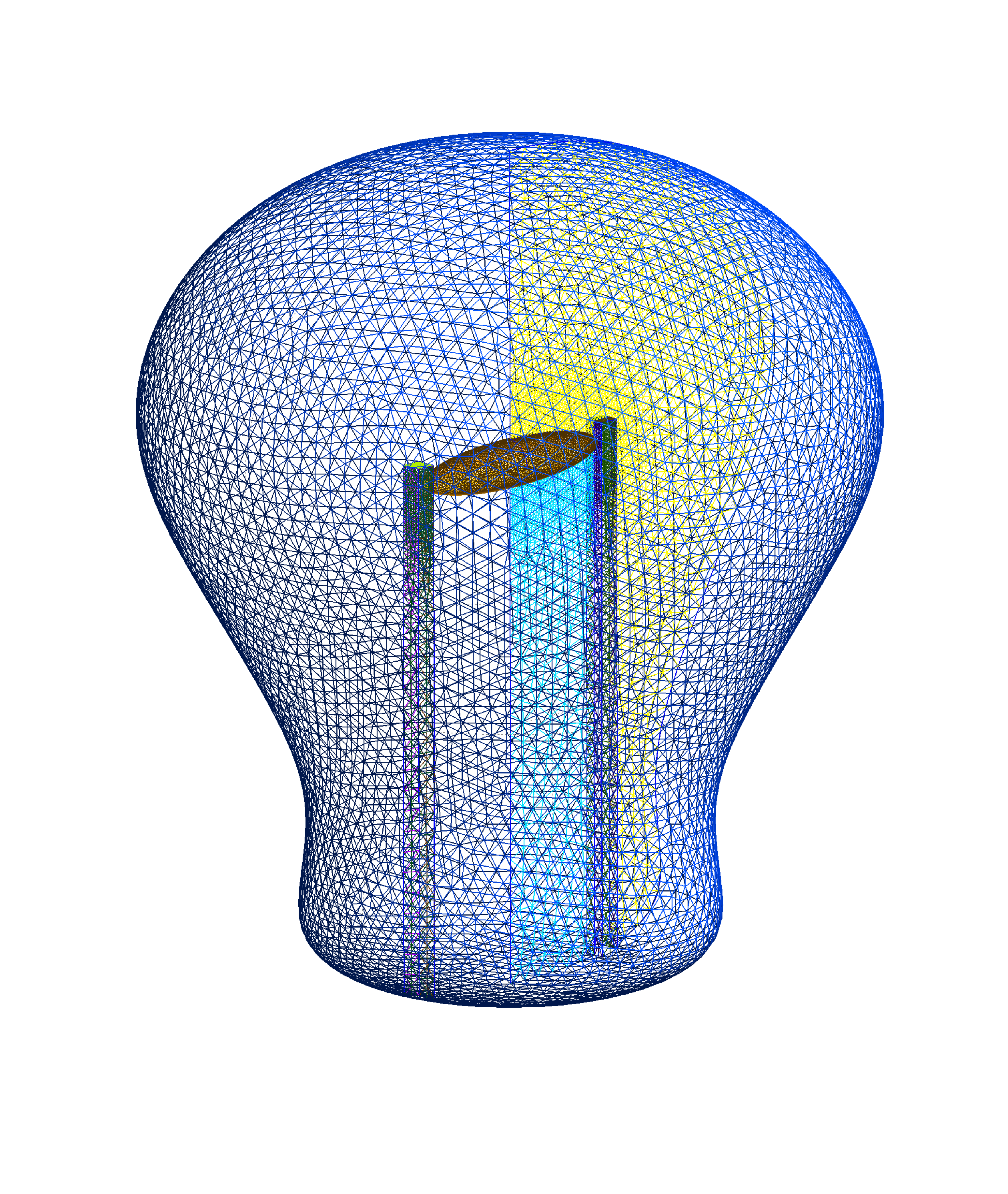
Figure 1: The finite element mesh and its boundary conditions for the convection-diffusion example.

The first example consists of solving a three-dimensional convection-diffusion equation over a domain $\Omega$

(25) $$\frac{\partial}{\partial t}u(\mathbf{x},t)=\nabla(\alpha\nabla u(\mathbf{x},t))+\beta\nabla u(\mathbf{x},t)+g(\mathbf{x},t),$$

for a time $t>0$, the space variable $\mathbf{x}=(x,y,z)\in\Omega$, a diffusion coefficient $\alpha$ and a convection coefficient $\beta$. In this example, we consider $\alpha,\beta$ constants in both time and space. For the problem to be well-defined, we set the initial condition as $u(\mathbf{x},0)=u_{0}(\mathbf{x})$ and impose some boundary conditions over $\partial\Omega$. After applying the standard Galerkin finite element procedure [30, 44] over the domain $\Omega$, we obtain the following system of equations:

(26) $$\mathbf{M}\frac{d}{dt}\mathbf{\hat{u}}=-\mathbf{A}\mathbf{\hat{u}}+\mathbf{M}\mathbf{g}(t),$$

where $\mathbf{M}$ is the mass matrix, $\mathbf{A}=\alpha\mathbf{D}+\beta\mathbf{C}$ is the stiffness matrix and $\mathbf{g}(t)$ is the load vector. Here, $\mathbf{D}$ and $\mathbf{C}$ correspond to the matrices related to the discretization of the diffusion and convection parts in the equation, respectively. We can then write the solution of (26) as

(27) $$\mathbf{\hat{u}}(t)=\exp(-\mathbf{L}\,t)\,\mathbf{\hat{u}}_{0}+\int_{0}^{t}\exp(-\mathbf{L}\,s)\,\mathbf{g}(t-s)\,ds.$$

with $\mathbf{L}=\mathbf{M}^{-1}\mathbf{A}$. To simplify the computation, we assume that the mass matrix $\mathbf{M}$ is lumped [30, 44], such that all of its mass is concentrated on the diagonal. We also assume that the load vector $\mathbf{g}$ remains constant through the entire simulation, such that the solution (27) can be simplified to

(28) $$\mathbf{\hat{u}}(t)=\exp(-\mathbf{L}\,t)\,\mathbf{\hat{u}}_{0}-\mathbf{L}^{-1}\exp(-\mathbf{L}\,t)\mathbf{g}+\mathbf{L}^{-1}\mathbf{g},$$

or, equivalently,

(29) $$\mathbf{\hat{u}}(t)=\mathbf{\hat{u}}_{0}+t\varphi_{1}(-\mathbf{L}t)\,\mathbf{b},\quad\varphi_{1}(z)=\frac{e^{z}-1}{z},$$

with $\mathbf{b}=\mathbf{g}-\mathbf{L}\mathbf{\hat{u}}_{0}$. $\varphi_{1}(z)$ is known as the “phi function” in the exponential integrator literature [28]. It is worth mentioning that evaluating (29) is more stable and faster than (28) as it avoids solving a linear system with $\mathbf{L}$, which can be quite problematic when $\mathbf{L}$ has an eigenvalue near the origin. This is not an issue when using (29) as $\varphi_{1}(z)$ is an entire function.

Fig. 1 shows the geometry of the domain used in this numerical experiment. The object has a finer discrete mesh near the boundary $\Gamma_{C}$ with the finite element size becoming larger as it moves in direction to the boundary $\Gamma_{A}$. The discrete mesh was generated with gmsh [21], while the mass and stiffness matrices were assembled using FreeFem++ [25] and P1 finite elements. We consider the following boundary conditions:

(30a) $$u(\mathbf{x},t)=0\quad\text{at}\quad x\in\Gamma_{A},$$

(30b) $$\nabla u(\mathbf{x},t)\cdot\mathbf{n}=0\quad\text{at}\quad x\in\Gamma_{B},$$

(30c) $$u(\mathbf{x},t)=1\quad\text{at}\quad x\in\Gamma_{C}.$$

Here, $\mathbf{n}$ denotes the outward normal vector to the boundary $\Gamma_{B}$. Let us assume that the rows of $\mathbf{L}$ are ordered such that the first $n_{i}$ rows corresponds to the nodes in the interior of $\Omega$ or on the boundary $\Gamma_{B}$, while the remaining $n_{b}$ rows correspond to the nodes at the boundaries $\Gamma_{A}$ and $\Gamma_{C}$. Then, to impose the boundaries conditions (30a) and (30c), we set the matrix $\mathbf{L}$, the load vector $\mathbf{g}$ and the initial conditions $\mathbf{u}_{0}$ as

$$\mathbf{L}=\begin{bmatrix}\mathbf{L}_{11}&\mathbf{L}_{12}\\ \mathbf{0}&\mathbf{I}\end{bmatrix}\qquad\mathbf{g}(\mathbf{x})=\begin{cases}1,\quad\mathbf{x}\in\Gamma_{C}\\ 0,\quad\text{otherwise}\end{cases}\qquad\mathbf{u}_{0}(\mathbf{x})=\begin{cases}0,\quad\mathbf{x}\in\Gamma_{A}\\ 1,\quad\mathbf{x}\in\Gamma_{C}\\ \xi,\quad\text{otherwise}\end{cases}$$

where $\mathbf{L}_{11}$ is the upper left $n_{i}\times n_{i}$ block from $\mathbf{L}$, $\mathbf{L}_{12}$ is the upper right $n_{i}\times n_{b}$ block from $\mathbf{L}$, $\mathbf{I}$ is the $n_{b}\times n_{b}$ identity matrix, and $\xi$ is random number drawn from the Gaussian distribution $\mathcal{N}(0.5,0.25)$. The Neumann boundary condition (30b) was satisfied during the assembly of the matrix $\mathbf{A}$.

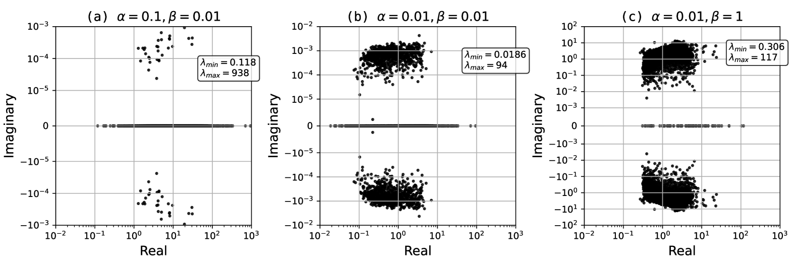
Figure 2: The spectrum of the matrix $\mathbf{L}$ for a coarse mesh with the size of the finite elements ranging between $0.12$ and $0.6$.

To gain some insight into the spectral properties of $\mathbf{L}$, we set the discrete mesh to be very coarse, such that the resulting matrix $\mathbf{L}$ is sufficiently small for its full eigendecomposition to be feasible. As shown in Fig. 2, the entire spectrum of $\mathbf{L}$ is located in the right half plane, which indicates that the solution (29) will converge to a steady state after a sufficiently long time $t$ has passed. If $\alpha\geq\beta$ (i.e., the diffusion term is equal or greater than the convection term), the majority of the eigenvalues of $\mathbf{L}$ are located near or at the real axis. If the dynamics of the problem are dominated by the convection (i.e., $\beta\gg\alpha$), most eigenvalues are complex with a large imaginary part. Generally speaking, the spectrum is wider for higher values of $\alpha$.

Table 1: Extremal eigenvalues and condition number of $\mathbf{L}$ for a mesh with a finite element size between $0.01$ and $0.05$.

	$\alpha$	$\beta$	$\lambda_{min}$	$\lambda_{max}$	$\sigma_{min}$	$\sigma_{max}$	$\kappa_{2}(\mathbf{A})$
Test (a)	$0.1$	$0.01$	$0.120$	$23,363$	$0.0706$	$25,842$	$365,898$
Test (b)	$0.01$	$0.01$	$0.0194$	$2,337$	$0.00813$	$2,585$	$317,921$
Test (c)	$0.01$	$1$	$1$	$2,437$	$0.0283$	$2,845$	$100,644$

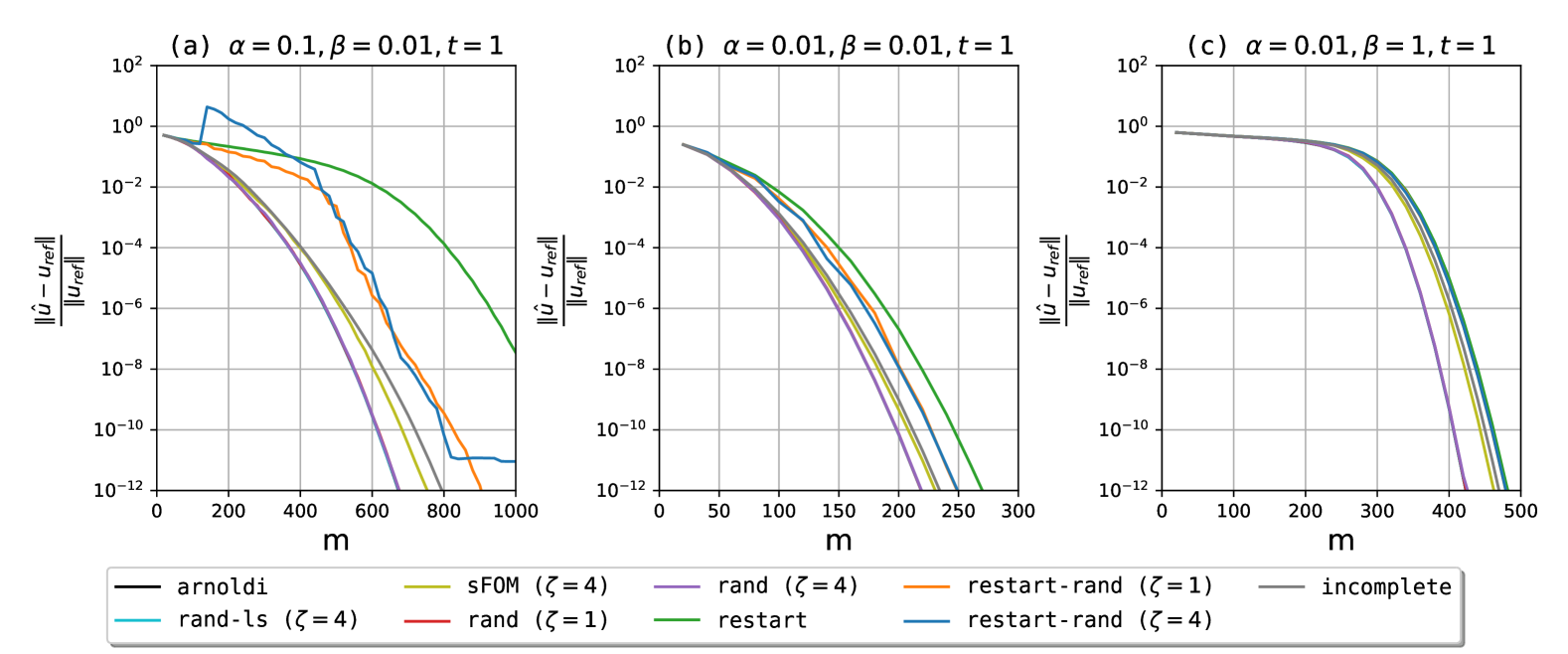
Figure 3: Convergence curves for different numerical methods when solving the convection-diffusion problem. Both the restart length $m_{r}$ and truncation parameter $k$ were set to $20$. In terms of the sketching dimension $d$, we set $d=2400$ for rand, rand-ls and sFOM and $d=320$ for restart-rand.

For the remaining numerical examples in this section, we consider a finite element size between $0.01$ and $0.05$, generating a matrix $\mathbf{L}$ with $4,801,565$ rows and $73,074,426$ nonzeros. Although the matrix is too large to compute the full eigendecomposition, we can estimate the extremal eigenvalues and singular values of $\mathbf{L}$ using ARPACK [31]. They are displayed in Table 1. We adopt as reference the solution obtained with the restart method with a tolerance of $3\times 10^{-12}$ and restart length $m_{r}=100$. The matrix phi-function $\varphi_{1}$ was calculated using the scaling-and-squaring method from [3, 26].

Fig. 3 shows the convergence curves for all numerical methods. From Table 1, we can infer that the spectrum of $\mathbf{L}$ in test (a) is significantly wider than others, and thus, it requires a much larger $m$ to approximate the entire spectrum. Likewise, assuming that the spectrum is similar to the examples plotted in Fig. 2, the complex eigenvalues in test (c) are farther away from the real axis than those in the other tests, which in turn slows down the convergence of the Krylov method.

In all examples, Algorithm 2 is able to produce a sufficiently well-conditioned Krylov basis $\mathbf{W}_{m}$, such that the errors of rand and rand-ls are virtually indistinguishable from the standard Arnoldi iteration (arnoldi), even with a small sparsity parameter $\zeta$. For instance, $\kappa_{2}(\mathbf{W}_{m})<8$ after $800$ iterations and only grows slightly between each iteration.

In contrast, with an incomplete orthogonalization, the Krylov basis $\mathbf{W}_{m}$ rapidly becomes ill-conditioned, reaching $\kappa_{2}(\mathbf{W}_{m})\geq 10^{15}$ after only $80$ iterations. As a result, incomplete converges significantly slower than arnoldi. The basis whitening in sFOM slightly improve the convergence rate, but it is not enough to match the other randomized methods. We observe that the incomplete method stagnates with $k=10$ and diverges with $k=5$ in test (a). The choice of $k$ only has a minor effect on the convergence of sFOM.

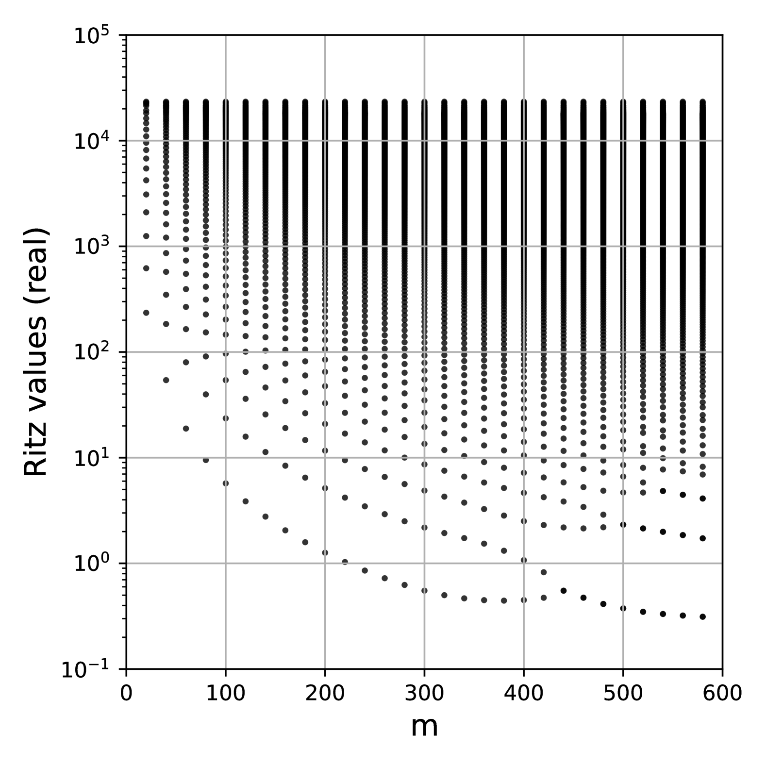
(a) arnoldi

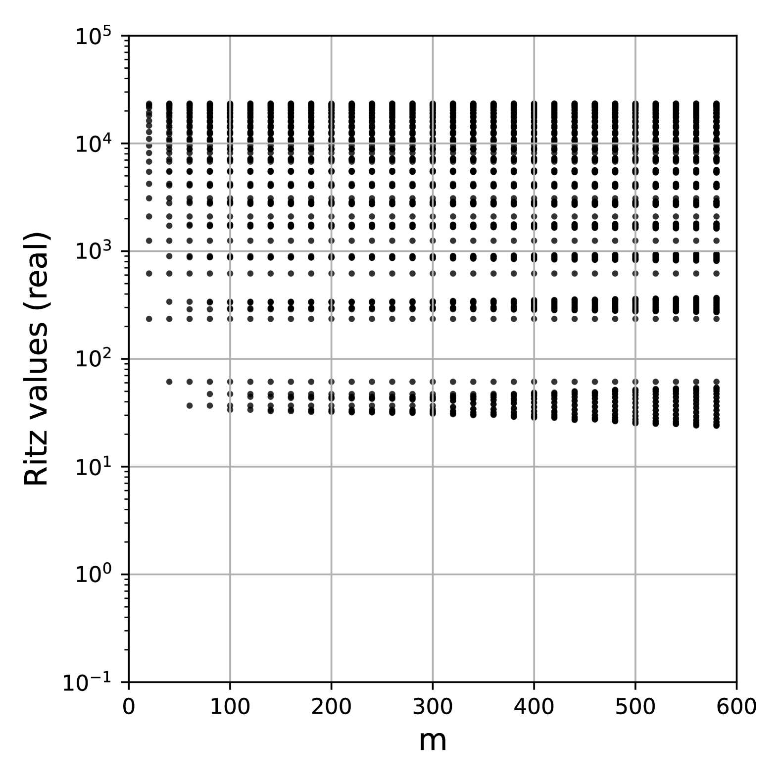
(b) restart

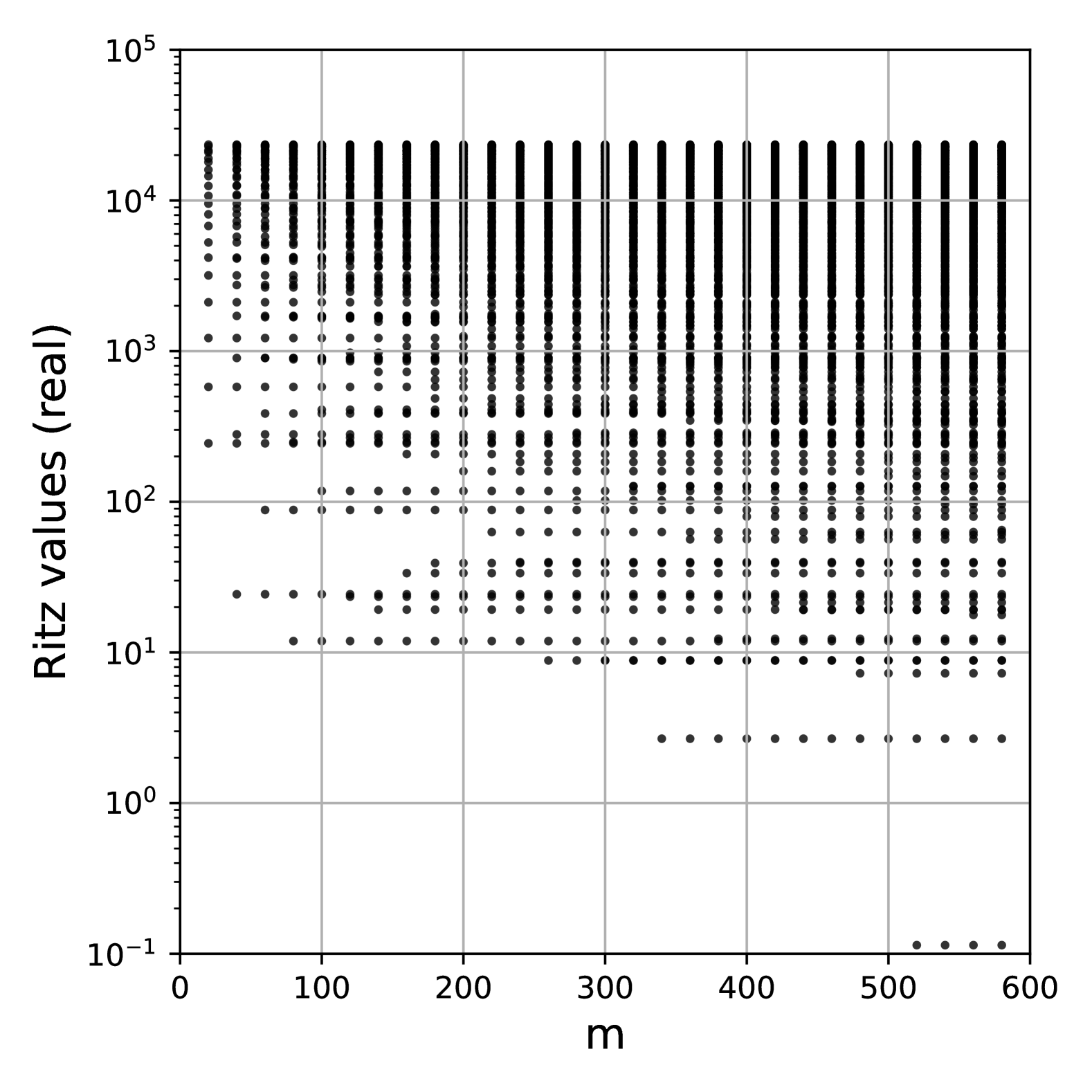
(c) restart-rand ($\zeta=1$)

Figure 4: The Ritz values for the convection-diffusion problem with $\alpha=0.1,\beta=0.01$, i.e., for test (a). The restart length was set to $20$.

As expected, restarting the Arnoldi procedure slows down the convergence of the method. Yet, surprisingly, restart-rand converges faster than standard restart with a significant lead in test (a). This can be explained in terms of the Ritz values as they determine the nodes of the underlying interpolation process from the Krylov approximant $\mathbf{f}_{m}\approx f(\mathbf{L})\mathbf{b}$ [14]. Fig. 4 shows the Ritz values from arnoldi, restart and restart-rand for test (a). Test (a) has a large value of $\alpha$, such that the spectrum of $\mathbf{L}$ is quite wide, ranging from $0.120$ to $23,363$ as shown in Table 1. Most eigenvalues of $\mathbf{L}$ are real or have a very small imaginary part.

After $m=600$ iterations, the Ritz values of arnoldi span the entire spectrum of $\mathbf{L}$ with the leftmost Ritz value located at $0.313$ (Fig. 4(a)). In contrast, restart has its Ritz values clustered around $20$ discrete points (see Fig. 4(b)), which is the same behavior observed in [1, 14, 15]. As a result, the minimum Ritz value of restart, located at $24.0$, is quite far away from the minimum eigenvalue of $\mathbf{L}$. The randomization in restart-rand introduces enough perturbation to the Ritz values to break the discrete behavior from restart. This leads to a better representation of the spectrum of $\mathbf{L}$ (Fig. 4(c)), such that now the leftmost Ritz value is located at $0.0.114$ after $m=600$ iterations. With $\zeta=4$, restart-rand shows an error spike around $m=140$ in test (a), but rapidly recovers its convergence towards the solution. It eventually stagnates around $10^{-11}$, which is near the tolerance of the reference solution. When using $\zeta=1$, restart-rand does not exhibit signs of instability.

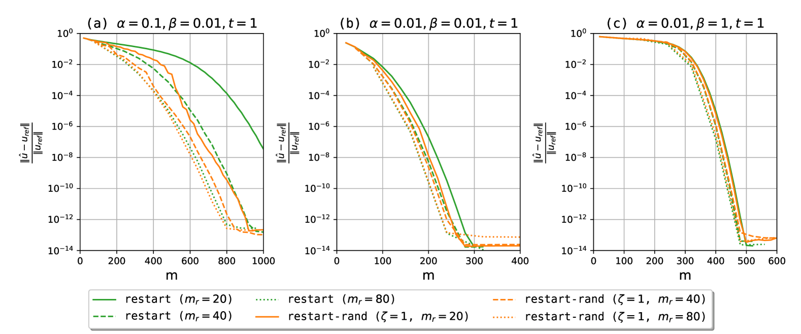
Figure 5: Convergence curves for restart and restart-rand for different restart lengths $m_{r}$ for the convection-diffusion example. The sketching dimension $d$ was set to $320$.

Fig. 5 shows the convergence curve of the restarted Krylov methods for different restart lengths $m_{r}$. Generally speaking, with a longer restart cycle (i.e., with a large $m_{r}$), the Ritz values are better distributed over the spectrum of $\mathbf{L}$, leading to a more accurate approximation of $f(\mathbf{L})\mathbf{b}$. Since $\mathbf{L}$ has the widest spectrum in test (a), we see a significant improvement in the convergence rate of the restarted methods after increasing the restart length $m_{r}$. In the other tests, a good representation of the spectrum of $\mathbf{L}$ is already attained with a restart length of $20$, and thus, increasing $m_{r}$ has a smaller impact on the convergence of the method compared to the test (a). The convergence of restart-rand can be slightly erratic due to randomization [39], especially for shorter restart lengths (i.e., with $m_{r}=20$). In all tests, the errors of restart-rand are equal to or lower than standard restart.

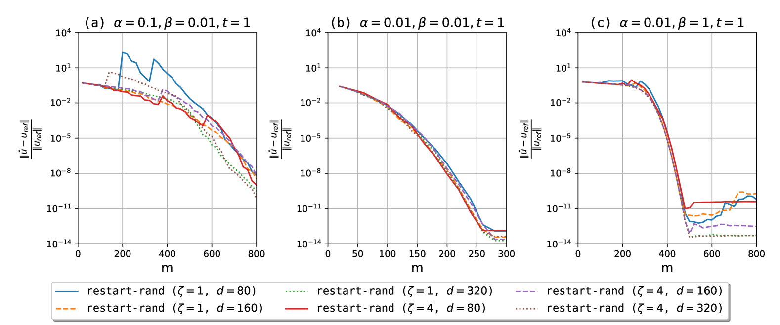
Figure 6: Convergence curves for restart-rand for different sketching dimensions $d$ for the convection-diffusion example. The restart length $m_{r}$ was set to $20$.

Fig. 6 shows the effect of the sketching dimension $d$ in the convergence of restart-rand. With $d\leq 160$, the sketch matrix $\mathbf{SW}_{m}$ does not contain enough information to build a fair representation of the Krylov basis $\mathbf{W}_{m}$ in each restart cycle. This causes the convergence of restart-rand to be quite erratic and may even lead to a temporary divergence, as seen in test (a). The method can also stagnate if the sketching dimension $d$ is too small, especially when the solution present an oscillatory behavior, e.g., in test (c). The stability do not seem to improve for $d\geq 320$.

5.2 Circular Membrane

The second example consists of simulating the vibrations of a circular membrane [38, Chapter 9]. Let us consider a membrane $\Omega$ of radius $\mu$ centred at the origin. At a time $t>0$, the height of the membrane in any point $(x,y)$ is given by $u(x,y,t)$, measured from the rest position. The membrane is attached to a rigid frame, such that $u(x,y,t)=0$ for $\forall x,y\in\partial\Omega$. The vibrations in the membrane can then be described as

(31) $$\frac{\partial^{2}}{\partial t^{2}}u(x,y,t)=-\nu^{2}\,\Delta u(x,y,t),$$

where $\nu>0$ is the speed at which the transversal waves propagate in the membrane. After using the finite element method [44] to describe (31) in terms of a discrete mesh over $\Omega$, we have

(32) $$\frac{d^{2}}{dt^{2}}\mathbf{\hat{u}}=-\nu^{2}\,\mathbf{L}\mathbf{\hat{u}},$$

where $\mathbf{L}=\mathbf{M}^{-1}\mathbf{A}$ for the stiffness matrix $\mathbf{A}$ and the lumped mass matrix $\mathbf{M}$. Suppose that the initial conditions are set to

(33) $$u(x,y,0)=J_{p}\left(\frac{\eta_{pk}\sqrt{x^{2}+y^{2}}}{\mu}\right),\qquad\frac{d}{dt}u(x,y,0)=0,$$

where $J_{p}(x)$ is the Bessel function

$$J_{p}(x)=\sum_{k=0}^{\infty}{\frac{(-1)^{k}}{k!\,(k+p)!}\left(\frac{x}{2}\right)^{2k+p}},$$

and $\eta_{pk}$ is the $k$-th zero of the $J_{p}(x)$. Then, the solution for (32) can be written as

(34) $$\mathbf{\hat{u}}(t)=\cos(\nu t\,\sqrt{\mathbf{L}})\,\mathbf{b},$$

where $\sqrt{\mathbf{L}}$ is any square root of $\mathbf{L}$ [20, p. 124] and $\mathbf{b}$ is a vector containing the value of $J_{p}(x)$ for each node in the discrete mesh. For our experiments, we consider a circular membrane with radius $\mu=1$ and set the initial conditions using a fourth-order Bessel function $J_{4}(x)$ and its fourth zero. The matrix $\mathbf{L}$ was generated with gmsh [21] and FreeFem++ [25] with a P1 finite element of size $0.0025$. To impose the Dirichlet boundary conditions $u(x,y,t)=0$ for $\forall x,y\in\partial\Omega$, we replace the corresponding rows of $\mathbf{L}$ with the identity matrix [30]. The resulting matrix $\mathbf{L}$ has $582,547$ rows and $4,062,636$ nonzeros. The maximum and minimum eigenvalues of $\mathbf{L}$ are $4.502\times 10^{6}$ and $1$, respectively. Its condition number $\kappa_{2}(\mathbf{L})$ is $7.11\times 10^{7}$. We adopted as reference the solution obtained by arnoldi with $m=2000$. The matrix cosine was computed using the scaling-and-squaring method from [4].

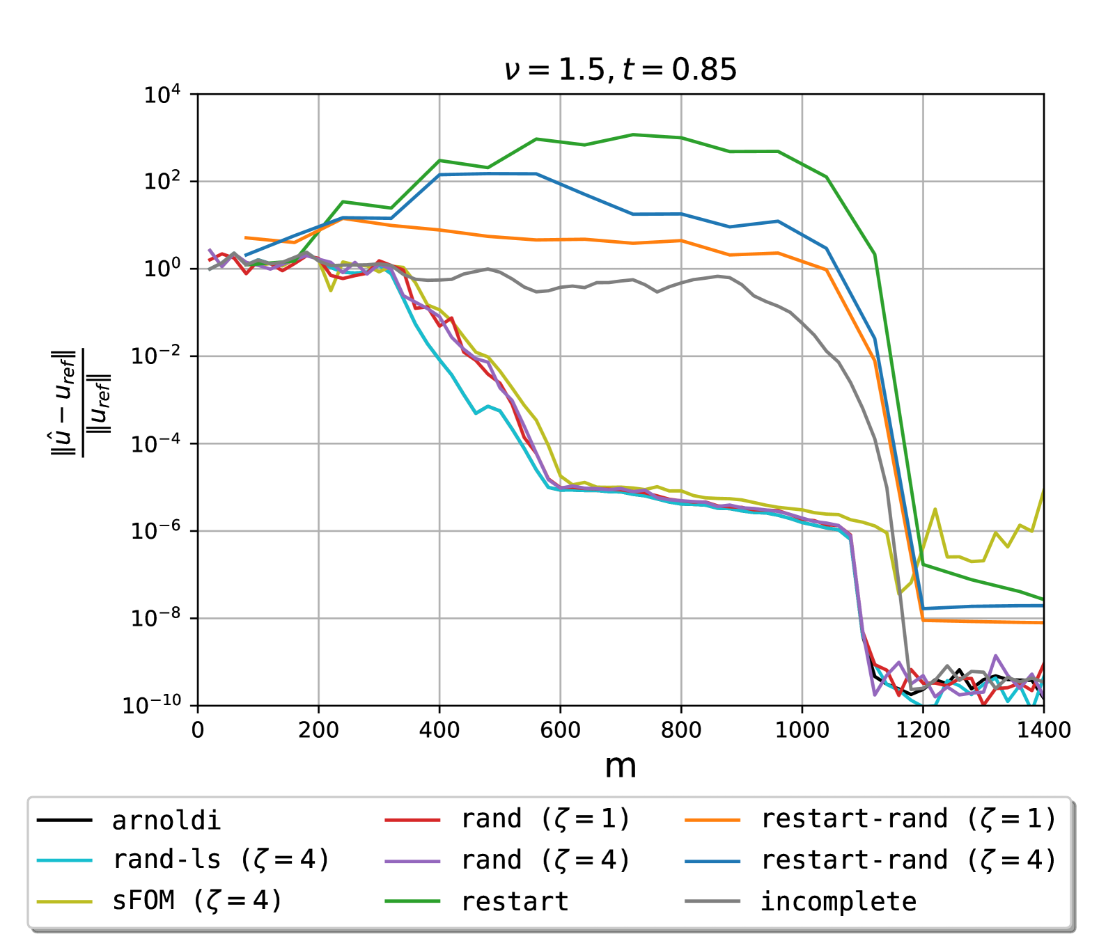
Figure 7: Convergence curves for different numerical methods when simulating the vibrations of a circular membrane. Both the restart length $m_{r}$ and truncation parameter $k$ were set to $80$. In terms of the sketching dimension $d$, we set $d=2800$ for rand, rand-ls and sFOM and $d=400$ for restart-rand.

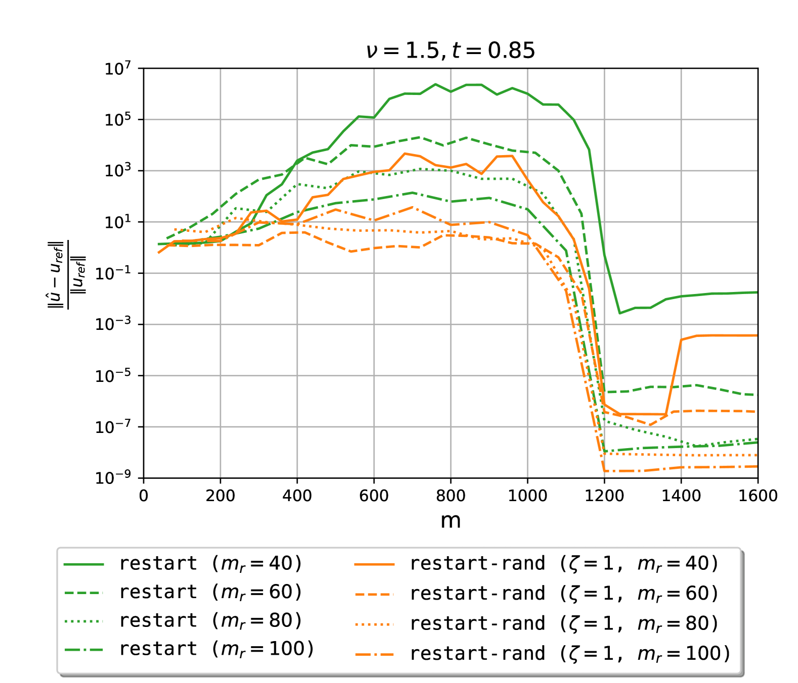
Figure 8: Convergence curves for restart and restart-rand for different restart lengths $m_{r}$ for the circular membrane example. The sketching dimension $d$ was set to $400$.

Fig. 8 shows the convergence curves for all numerical methods. As a consequence of the oscillatory nature of the problem, the classical arnoldi method has a stairway-shaped convergence and eventually stagnates around $10^{-10}$ after $m=1200$ iterations. The errors of rand and rand-ls closely follow those from the classical method, while incomplete takes around $m=900$ iterations to start converging to the solution. It achieves the same accuracy as the other methods at the end of the experiment. For the first $m=1040$ iterations, the error of sFOM is quite similar to the other randomized methods, but starts to diverge afterwards. The minimum error obtained by sFOM was $3.612\times 10^{-8}$.

For the first $12$ restarts (i.e., $m\leq 960$), the errors of restart and restart-rand are quite large, showing signs of instability. After that, they start to converge rapidly toward the solution but reach another plateau at $10^{-8}$. The final accuracy is primarily dictated by the restart length $m_{r}$ as shown in Fig. 8. It also controls how far away the method diverges from the reference solution. In general, the error of restart-rand is better than restart, although it still shows similar signs of instability.

After experimenting with different sketching dimensions $d$, we found out that the accuracy of restart-rand does not improve for $d>600$. At the same time, the method has low accuracy with $d<400$. Similarly, the errors of rand, rand-ls and sFOM do not improve by increasing the sketching dimension beyond $2800$.

5.3 Performance

Fig. 9 compares the execution time and accuracy of the numerical methods. For the conv-diff test (a-c), we set $m_{r}=k=20$; $d=2400$ for rand, rand-ls and sFOM; and $d=320$ for restart-rand. For the membrane test (d), $m_{r}=k=80$; $d=2800$ for rand, rand-ls and sFOM; and $d=400$ for restart-rand. The number of restarts and the basis size $m$ were adjusted in such a way that all methods have similar accuracy. The experiments were run on a single thread to avoid performance issues that arise during the parallelization.

In all tests, arnoldi has the highest execution time among all methods due to the full orthogonalization of the Krylov basis. Replacing the classical Arnoldi procedure with the randomized version (i.e., the rand method) leads to a speedup of up to $2.68$ and $2.92$ for $\zeta=4$ and $\zeta=1$, respectively. The performance gap between rand and arnoldi increases for larger values of $m$. In addition to the lower cost, the randomized Arnoldi has a few other attributes that result in faster execution times. In particular, the method may have better memory access times as the sketch $\mathbf{SW}_{m}$ is sufficiently small to fit in the L3 cache. For example, a $2400\times 800$ matrix $\mathbf{SW}_{m}$ consumes around $15$MB, while the AMD 7H12 CPU has $16$MB of L3 cache per CCX. Moreover, Algorithm 2 updates the basis $\mathbf{W}_{m}$ using a single BLAS-2 routine (gemv) instead of multiple calls to BLAS-1 routines (axpy and dot) like in the standard Arnoldi. Solving the least square problem using LSMR for rand-ls imposes a $10$ to $15\%$ performance penalty depending on the size of the input matrix and Krylov basis.

With a restarted Krylov method, the program spent significantly less time in the orthogonalization of the basis since it only needs to work with a small set of basis vectors at each restart cycle. As a result, the faster orthogonalization in Algorithm 2 has less impact on the overall performance of the program and it may be overshadowed by the overhead of constructing the sketch $\mathbf{SW}_{m}$. This is the case for tests (b) and (c), where the restart length is very short ($m_{r}=20$), such that restart-rand with $\zeta=4$ has very similar performance than restart. Reducing the sparsity parameter to $\zeta=1$, restart-rand become around $15\%$ faster due to lower sketching cost. In contrast, for the test (a), restart-rand shows a speedup of $1.29$ and $1.56$ over the standard restart method with $\zeta=4$ and $\zeta=1$, respectively. Recall from Section 5.1 that the convergence rate of restart-rand is significantly higher than restart in test (a), and thus, requires fewer restarts to achieve the same accuracy. Finally, in test (d), the restarted methods require a longer cycle ($m_{r}=80$) to be stable and the input matrix is smaller (i.e., lower sketching cost). As a result, with $\zeta=1$, restart-rand is around $1.55\times$ faster than restart, while being $10\times$ more accurate. It is worth mentioning that restart can only match the accuracy of restart-rand by increasing the restart length, which further widens the performance gap between the randomized and the classical method.

With an incomplete orthogonalization, both incomplete and sFOM have a fixed cost for building the basis regardless of its size, but require a larger number of iterations to achieve the target accuracy. As a result, the performance of incomplete is similar to the restarted procedures. sFOM is significantly slower than incomplete due to the relatively high cost of the basis whitening process. In test (c), the maximum accuracy attained by sFOM is $1.34\times 10^{-6}$, while the error of the other methods is below $10^{-8}$. The only exception is restart which has an error of $8.74\times 10^{-8}$.

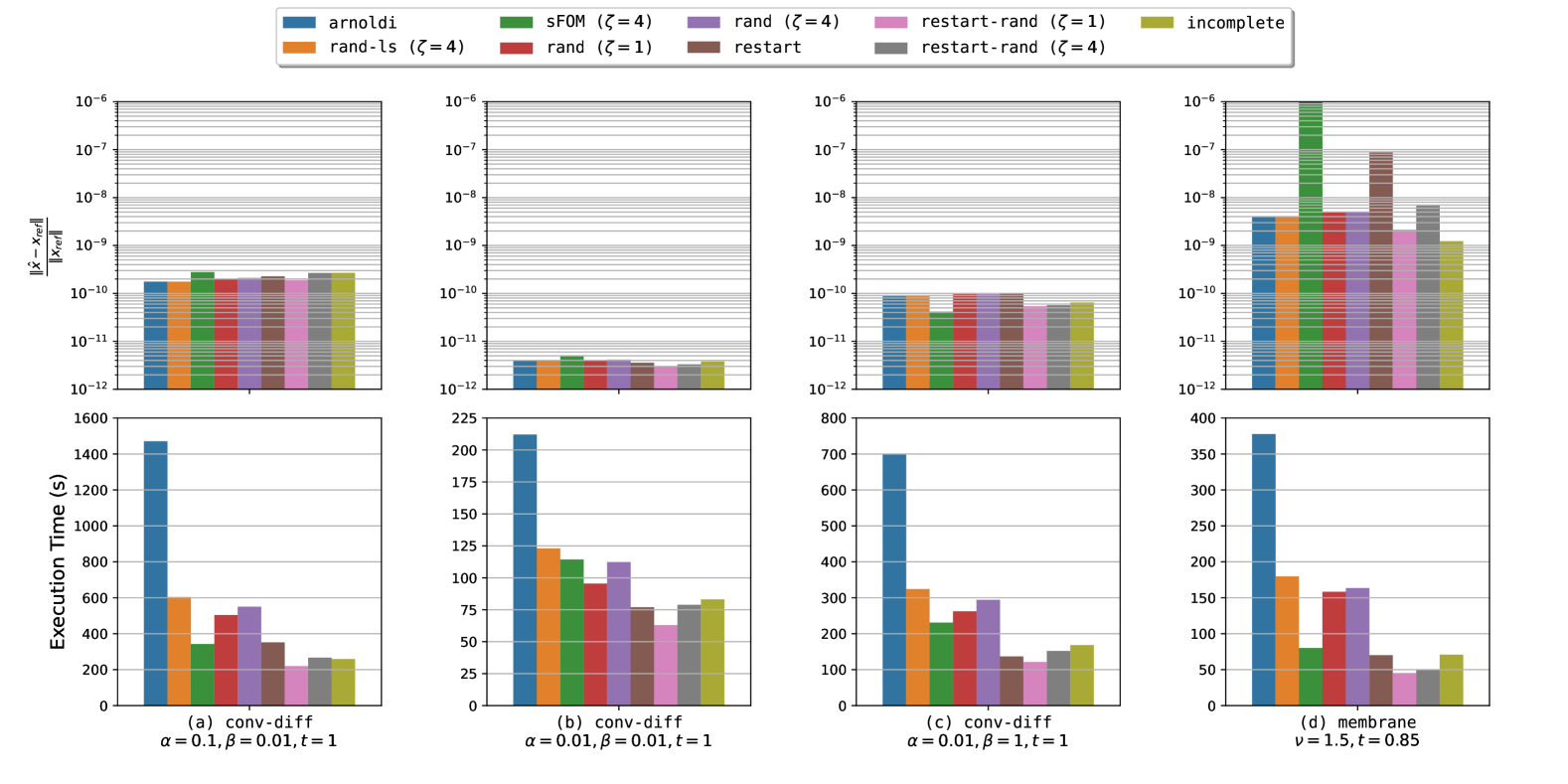
Figure 9: Comparison between the serial execution time and accuracy of the different Krylov methods.

6 Conclusion

In this article, we propose a new acceleration technique based on random sketching for restarted Krylov methods in the context of general matrix functions. Our numerical experiments show that our randomized algorithm significantly outperforms the classical method while producing a highly accurate solution for complex finite element problems. In some cases, the randomization can even lead to better convergence rates for the restarted method.

Although our randomized method performs well in practice, many features of these methods are not completely understood. In particular, a formal explanation of how the randomization affects the spectral properties of the method is still missing. This can help us understand why randomization is very effective for accelerating the convergence in some problems while showing minor improvement for others. Likewise, a stronger theory for the convergence of randomized methods may lead to a better error estimation, allowing greater control over the number of restarts.

As future work, we can also explore other acceleration techniques, such as spectral deflation [15], weighted inner products [16] or “thick” restarting [6], to further improve the performance of our randomized method.

Code Availability

The code for running the numerical examples can be found at https://gitlab.com/nlg550/randomized-krylov.

References

- [1] M. Afanasjew, M. Eiermann, O. Ernst, and A. Uttel, A generalization of the steepest descent method for matrix functions, Electronic Transactions on Numerical Analysis. Volume, 28 (2008), pp. 206–222.
- [2] M. Afanasjew, M. Eiermann, O. G. Ernst, and S. Güttel, Implementation of a restarted Krylov subspace method for the evaluation of matrix functions, Linear Algebra and its Applications, 429 (2008), pp. 2293–2314, https://doi.org/10.1016/j.laa.2008.06.029.
- [3] A. H. Al-Mohy and N. J. Higham, A New Scaling and Squaring Algorithm for the Matrix Exponential, SIAM Journal on Matrix Analysis and Applications, 31 (2010), pp. 970–989, https://doi.org/10.1137/09074721X.
- [4] A. H. Al-Mohy, N. J. Higham, and S. D. Relton, New Algorithms for Computing the Matrix Sine and Cosine Separately or Simultaneously, SIAM Journal on Scientific Computing, 37 (2015), pp. A456–A487, https://doi.org/10.1137/140973979.
- [5] H. Avron, P. Maymounkov, and S. Toledo, Blendenpik: Supercharging LAPACK’s Least-Squares Solver, SIAM Journal on Scientific Computing, 32 (2010), pp. 1217–1236, https://doi.org/10.1137/090767911.
- [6] A. H. Baker, E. R. Jessup, and T. Manteuffel, A Technique for Accelerating the Convergence of Restarted GMRES, SIAM Journal on Matrix Analysis and Applications, 26 (2005), pp. 962–984, https://doi.org/10.1137/S0895479803422014.
- [7] O. Balabanov and L. Grigori, Randomized Gram–Schmidt Process with Application to GMRES, SIAM Journal on Scientific Computing, 44 (2022), pp. A1450–A1474, https://doi.org/10.1137/20M138870X.
- [8] M. Benzi and P. Boito, Matrix functions in network analysis, GAMM-Mitteilungen, 43 (2020), p. e202000012, https://doi.org/10.1002/gamm.202000012.
- [9] M. Benzi and I. Simunec, Rational Krylov methods for fractional diffusion problems on graphs, BIT Numerical Mathematics, 62 (2022), pp. 357–385, https://doi.org/10.1007/s10543-021-00881-0.
- [10] J. C. R. Bloch and S. Heybrock, A nested Krylov subspace method to compute the sign function of large complex matrices, Computer Physics Communications, 182 (2011), pp. 878–889, https://doi.org/10.1016/j.cpc.2010.09.022.
- [11] R.-U. Börner, O. G. Ernst, and S. Güttel, Three-dimensional transient electromagnetic modelling using Rational Krylov methods, Geophysical Journal International, 202 (2015), pp. 2025–2043, https://doi.org/10.1093/gji/ggv224.
- [12] M. B. Cohen, Nearly Tight Oblivious Subspace Embeddings by Trace Inequalities, in Proceedings of the Twenty-Seventh Annual ACM-SIAM Symposium on Discrete Algorithms, Society for Industrial and Applied Mathematics, Jan. 2016, pp. 278–287, https://doi.org/10.1137/1.9781611974331.ch21.
- [13] A. Cortinovis, D. Kressner, and Y. Nakatsukasa, Speeding Up Krylov Subspace Methods for Computing f(A)b via Randomization, SIAM Journal on Matrix Analysis and Applications, 45 (2024), pp. 619–633, https://doi.org/10.1137/22M1543458.
- [14] M. Eiermann and O. G. Ernst, A Restarted Krylov Subspace Method for the Evaluation of Matrix Functions, SIAM Journal on Numerical Analysis, 44 (2006), pp. 2481–2504, https://doi.org/10.1137/050633846.
- [15] M. Eiermann, O. G. Ernst, and S. Güttel, Deflated Restarting for Matrix Functions, SIAM Journal on Matrix Analysis and Applications, 32 (2011), pp. 621–641, https://doi.org/10.1137/090774665.
- [16] M. Embree, R. B. Morgan, and H. V. Nguyen, Weighted Inner Products for GMRES and GMRES-DR, SIAM Journal on Scientific Computing, 39 (2017), pp. S610–S632, https://doi.org/10.1137/16M1082615.
- [17] D. C.-L. Fong and M. Saunders, LSMR: An Iterative Algorithm for Sparse Least-Squares Problems, SIAM Journal on Scientific Computing, 33 (2011), pp. 2950–2971, https://doi.org/10.1137/10079687X.
- [18] A. Frommer, S. Güttel, and M. Schweitzer, Convergence of Restarted Krylov Subspace Methods for Stieltjes Functions of Matrices, SIAM Journal on Matrix Analysis and Applications, 35 (2014), pp. 1602–1624, https://doi.org/10.1137/140973463.
- [19] A. Frommer, S. Güttel, and M. Schweitzer, Efficient and Stable Arnoldi Restarts for Matrix Functions Based on Quadrature, SIAM Journal on Matrix Analysis and Applications, 35 (2014), pp. 661–683, https://doi.org/10.1137/13093491X.
- [20] F. R. Gantmakher, The Theory of Matrices, vol. 1, Chelsea Publishing Company, New York, NY, 1959.
- [21] C. Geuzaine and J.-F. Remacle, Gmsh: A 3-D finite element mesh generator with built-in pre- and post-processing facilities, International Journal for Numerical Methods in Engineering, 79 (2009), pp. 1309–1331, https://doi.org/10.1002/nme.2579.
- [22] S. Güttel, Rational Krylov approximation of matrix functions: Numerical methods and optimal pole selection, GAMM-Mitteilungen, 36 (2013), pp. 8–31, https://doi.org/10.1002/gamm.201310002.
- [23] S. Güttel, D. Kressner, and K. Lund, Limited-memory polynomial methods for large-scale matrix functions, GAMM-Mitteilungen, 43 (2020), p. e202000019, https://doi.org/10.1002/gamm.202000019.
- [24] S. Güttel and M. Schweitzer, Randomized Sketching for Krylov Approximations of Large-Scale Matrix Functions, SIAM Journal on Matrix Analysis and Applications, 44 (2023), pp. 1073–1095, https://doi.org/10.1137/22M1518062.
- [25] F. Hecht, New development in freefem++, Journal of Numerical Mathematics, 20 (2012), pp. 251–266, https://doi.org/10.1515/jnum-2012-0013.
- [26] N. J. Higham, The Scaling and Squaring Method for the Matrix Exponential Revisited, SIAM Journal on Matrix Analysis and Applications, 26 (2005), pp. 1179–1193, https://doi.org/10.1137/04061101X.
- [27] N. J. Higham, Functions of Matrices, Other Titles in Applied Mathematics, Society for Industrial and Applied Mathematics, Philadelphia, PA, Jan. 2008, https://doi.org/10.1137/1.9780898717778.
- [28] M. Hochbruck and A. Ostermann, Exponential integrators, Acta Numerica, 19 (2010), pp. 209–286, https://doi.org/10.1017/S0962492910000048.
- [29] C. Lanczos, An iteration method for the solution of the eigenvalue problem of linear differential and integral operators, Journal of Research of the National Bureau of Standards, 45 (1950), p. 255, https://doi.org/10.6028/jres.045.026.
- [30] M. G. Larson and F. Bengzon, The Finite Element Method: Theory, Implementation, and Applications, vol. 10 of Texts in Computational Science and Engineering, Springer, Berlin, Heidelberg, 2013, https://doi.org/10.1007/978-3-642-33287-6.
- [31] R. B. Lehoucq, ARPACK Users’ Guide: Solution of Large-Scale Eigenvalue Problems with Implicitly Restarted Arnoldi Methods, no. 6 in Software, Environments, Tools, Society for Industrial and Applied Mathematics, Philadelphia, Pa, 1998, https://doi.org/10.1137/1.9780898719628.
- [32] P.-G. Martinsson and J. A. Tropp, Randomized numerical linear algebra: Foundations and algorithms, Acta Numerica, 29 (2020), pp. 403–572, https://doi.org/10.1017/S0962492920000021.
- [33] Y. Nakatsukasa and J. A. Tropp, Fast and Accurate Randomized Algorithms for Linear Systems and Eigenvalue Problems, SIAM Journal on Matrix Analysis and Applications, 45 (2024), pp. 1183–1214, https://doi.org/10.1137/23M1565413.
- [34] C. C. Paige and M. A. Saunders, LSQR: An Algorithm for Sparse Linear Equations and Sparse Least Squares, ACM Transactions on Mathematical Software, 8 (1982), pp. 43–71, https://doi.org/10.1145/355984.355989.
- [35] D. Palitta, M. Schweitzer, and V. Simoncini, Sketched and Truncated Polynomial Krylov Methods: Evaluation of Matrix Functions, Numerical Linear Algebra with Applications, 32 (2025), p. e2596, https://doi.org/10.1002/nla.2596.
- [36] Y. Saad, Iterative Methods for Sparse Linear Systems, Other Titles in Applied Mathematics, Society for Industrial and Applied Mathematics, Jan. 2003, https://doi.org/10.1137/1.9780898718003.
- [37] W. E. Schiesser, The Numerical Method of Lines: Integration of Partial Differential Equations, Elsevier, San Diego, CA, 1st ed., June 1991.
- [38] J. W. Strutt, The Theory of Sound, vol. 1 of Cambridge Library Collection - Physical Sciences, Cambridge University Press, Cambridge, 2011, https://doi.org/10.1017/CBO9781139058087.
- [39] E. Timsit, L. Grigori, and O. Balabanov, Randomized Orthogonal Projection Methods for Krylov Subspace Solvers, Mar. 2023, https://doi.org/10.48550/arXiv.2302.07466, https://arxiv.org/abs/2302.07466.
- [40] J. A. Tropp, A. Yurtsever, M. Udell, and V. Cevher, Streaming Low-Rank Matrix Approximation with an Application to Scientific Simulation, SIAM Journal on Scientific Computing, 41 (2019), pp. A2430–A2463, https://doi.org/10.1137/18M1201068.
- [41] J. van den Eshof, A. Frommer, Th. Lippert, K. Schilling, and H. A. van der Vorst, Numerical methods for the QCD overlap operator. I. Sign-function and error bounds, Computer Physics Communications, 146 (2002), pp. 203–224, https://doi.org/10.1016/S0010-4655(02)00455-1.
- [42] J. H. Wilkinson, The Calculation of the Eigenvectors of Codiagonal Matrices, The Computer Journal, 1 (1958), pp. 90–96, https://doi.org/10.1093/comjnl/1.2.90.
- [43] D. P. Woodruff, Sketching as a Tool for Numerical Linear Algebra, Foundations and Trends® in Theoretical Computer Science, 10 (2014), pp. 1–157, https://doi.org/10.1561/0400000060.
- [44] O. C. Zienkiewicz, R. L. Taylor, and J. Z. Zhu, The Finite Element Method: Its Basis and Fundamentals, Elsevier, Kidlington, Oxfor, 7nd ed., Aug. 2013.