Interpretable Deep Learning Paradigm for Airborne Transient Electromagnetic Inversion

Abstract

We established a unified and interpretable deep learning inversion paradigm for ATEM inversion based on disentangled representation learning. The network demonstrates the ability to decouple noisy data into noise and signal factors, using only the signal factor for inversion. This approach unifies the denoising and inversion processes for real-world data while incorporating physical information as guidance. By completing the entire data processing procedure based on the signal factor, the network yields more reliable and interpretable results. The inversion results on real-world data indicate that our method can directly utilize noisy data to accurately reconstruct the subsurface electrical structure. Moreover, it can handle data affected by significant environmental noise, which traditional methods struggle with, thereby achieving a better lateral structural resolution.

Key Laboratory of Earth Exploration and Information Techniques Ministry of Education, College of Geophysics, Chengdu University of Technology, Chengdu, China College of Computer Science and Cyber Security, Chengdu University of Technology, Chengdu, China College of Computer Science, Chengdu University, Chengdu, China

Xiaodong Yuyuxiaodong@cdu.edu.cn

We propose an interpretable deep learning inversion paradigm that enables accurate inversion.

By leveraging disentangled representation learning, we unify the denoising and inversion processes for field data, simplifying the overall data processing workflow and improving efficiency.

The network incorporates physical information as guidance and completes the entire data processing procedure based on the signal factor, enhancing both the reliability and interpretability of the results.

Plain Language Summary

The primary process of extracting geoelectric structural information from airborne transient electromagnetic (ATEM) data consists of data processing and inversion. Traditional methods struggle to handle complex field data with significant noise. Existing deep learning approaches treat denoising and inversion as separate processes, and independently trained denoising networks often fail to ensure the reliability of subsequent inversion. To address this issue, we established a unified and interpretable deep learning inversion paradigm based on disentangled representation learning. The network decouples noisy data into noise and signal factors, completing the entire data processing procedure using only the signal factor while incorporating physical information as guidance. This approach enhances the reliability and interpretability of the network’s results. The inversion results on real-world data demonstrate that our method can directly utilize noisy data to accurately reconstruct the subsurface electrical structure. Furthermore, it can effectively handle data influenced by significant environmental noise, which traditional methods struggle with, thereby achieving improved lateral structural resolution.

1 Introduction

The airborne transient electromagnetic (ATEM) method is a widely used technique in electromagnetic detection and a current focal point of research in geological exploration. It involves a transmitting loop that generates a time-varying current during flight, while receiving coils capture the induced secondary electromagnetic field produced by subsurface media to map underground structures [Palacky  West (1991)]. By mounting both the transmitting and receiving systems on the aircraft, ATEM facilitates rapid coverage of extensive and difficult-to-reach survey areas. It has been widely applied in geohazards investigations [Damhuis . (2020), Malehmir . (2016)], groundwater resource exploration [Ball . (2020), Minsley . (2021)], mineral prospecting [Koné . (2021), Okada (2021)], and geological mapping [Dzikunoo . (2020), Wong . (2020)].

The primary process of extracting geoelectric structural information from ATEM data involves data processing and inversion [X. Wu . (2022)]. The core task of data processing, beyond steps such as system response effect removal, is denoising. Due to the dynamic nature of data acquisition, complex noise conditions, long observation distances, and relatively weak signal strength, ATEM data processing presents significant challenges [X. Wu . (2019)]. Traditional physics-based methods, including principal component analysis [Asten (2009)], stationary wavelet transform [Li . (2017)], singular value decomposition [Reninger . (2011)], and ensemble empirical mode decomposition [F. Liu . (2017)], typically rely on the selection of empirical parameters. This limitation not only demands significant operator expertise but also restricts their effectiveness primarily to low-noise scenarios. Current field applications reveal notable performance degradation when these conventional approaches encounter complex geological environments with elevated noise contamination levels, particularly in challenging survey conditions involving strong electromagnetic interference and low signal-to-noise ratios [X. Wu . (2020)].

Inversion directly reflects the geoelectric structure. Conventional inversion methods, such as the Occam inversion method [Constable . (1987), Vallée  Smith (20091)] and some regularized approaches [Siemon . (2009), Vallée  Smith (20092), Vignoli . (2015), Christensen . (2017)], rely on forward modeling to iteratively refine the inversion results [Bai . (2021)]. This process is computationally expensive, with costs increasing geometrically as the number of observations grows, making it prohibitively expensive for large-scale datasets. Moreover, due to noise and the inherent non-uniqueness of inverse problems, regularization methods require relatively accurate prior information (initial models) of the subsurface structure, often encountering challenges with multiple local minima [K. Cheng . (20242)]. Probabilistic inversion methods, such as Bayesian-based approaches, provide a probability distribution of resistivity values, transforming the inversion problem into one of determining the probability distribution of inversion parameters [K. Cheng . (20242)]. While this method is suitable for highly nonlinear problems, however, its computational cost is high and increases exponentially with the number of model parameters [S. Wu . (2023)].

With the advancement of deep learning, its application in denoising and inversion of geophysical data has attracted significant attention as a means of overcoming the limitations of traditional methods. For example, denoising autoencoders have been used to remove multi-source noise from data [X. Wu . (2020)]; one-dimensional signals have been transformed into two-dimensional sequences for transient electromagnetic denoising using image denoising networks [Chen . (2020)]; wu2021noising employed a Long Short-Term Memory (LSTM) network combined with an autoencoder structure to denoise data. liu2024multi proposed a Transformer-based multi-task learning network architecture for denoising data. cheng2025pc utilized parallel convolution to extract multi-scale features from input data and then applied a bidirectional Long Short-Term Memory (BiLSTM) network to establish complex mapping relationships between features and clean data for transient electromagnetic denoising. Additionally, data-driven convolutional neural network (CNN)-based inversion has been employed [S. Wu . (20211)], LSTM utilized for fast inversion [S. Wu . (2022)]. wu2024physics developed a hybrid deep learning-based method that integrates deep learning-based forward modeling losses into the loss function to yield more consistent inversion results. kang2024deep designed a deep learning-based inversion process, while zhang2024airborne introduced a multi-input, single-output double-hidden wavelet neural network for ATEM data imaging. cheng2024multi proposed a TEM inversion algorithm based on a multi-scale expanded convolutional neural network, aiming to fully exploit the multi-scale information in the data to improve inversion reliability. Furthermore, cheng2024transient proposed an inversion method using CNN-LightGBM. However, these deep learning approaches treat denoising and inversion as separate processes, thereby creating a distinct boundary between them. This separation necessitates the training of two independent networks—one for denoising and another for inversion. Since inversion is a downstream task that heavily depends on the accuracy of the denoising results, it typically evaluates the reliability of the estimated model by calculating the deviation between the model’s response and the processed data, but it cannot simultaneously assess the ”purity” of the processed data. As a result, if residual interference remains in the processed data, the reliability of the inversion is compromised [X. Wu . (2022)]. Moreover, training two separate networks requires significant computational resources and time, and existing networks with end-to-end outputs often lack interpretability.

To address the aforementioned challenges, we propose a unified and interpretable deep learning inversion paradigm based on disentangled representation learning. The network effectively decouples noisy data into noise and signal factors, using the signal factors for inversion. This approach integrates denoising and inversion processes for field data, streamlining the overall data processing workflow and enhancing efficiency. The network incorporates physical information as guidance, completing the entire data processing procedure based on the signal factors, thereby improving both the reliability and interpretability of the results. Inversion results on field data demonstrate that our model can efficiently and accurately reconstruct the subsurface electrical structure without the need for manual data preprocessing.

2 Method

Existing deep learning methods are typically designed for specific stages of the data processing pipeline, such as denoising or inversion, without integrating both processes into a unified framework. However, because inversion inherently depends on denoised data, integrating these two stages can streamline the entire workflow.

Disentangled representation learning seeks to model key representations within data by separating task-relevant factors from task-irrelevant ones [Wang . (2024)]. In the context of denoising and inversion, the useful data representation within the signal corresponds to task-relevant factors, while noise represents task-irrelevant factors. Since the task-relevant factors for both denoising and inversion are the same—referred to as the signal factor—we leverage disentangled representation learning to decouple data into signal and noise factors, performing inversion based on the signal factor. This approach seamlessly integrates denoising and inversion into a unified framework. Additionally, we employ a data decoder to ensure that the encoder correctly disentangles the data. The overall framework is depicted in Fig. 1.

Figure 1: The overall framework, the data is encoded by the encoder $E$ into signal and noise factors. The inversion decoder $G_{r}$ decodes the signal factor to obtain accurate inversion results. $G_{s}$ is used to decode the combination of signal and noise factors into the signal, ensuring the correct disentangled representation. The loss function incorporates physical information to impose physical constraints.

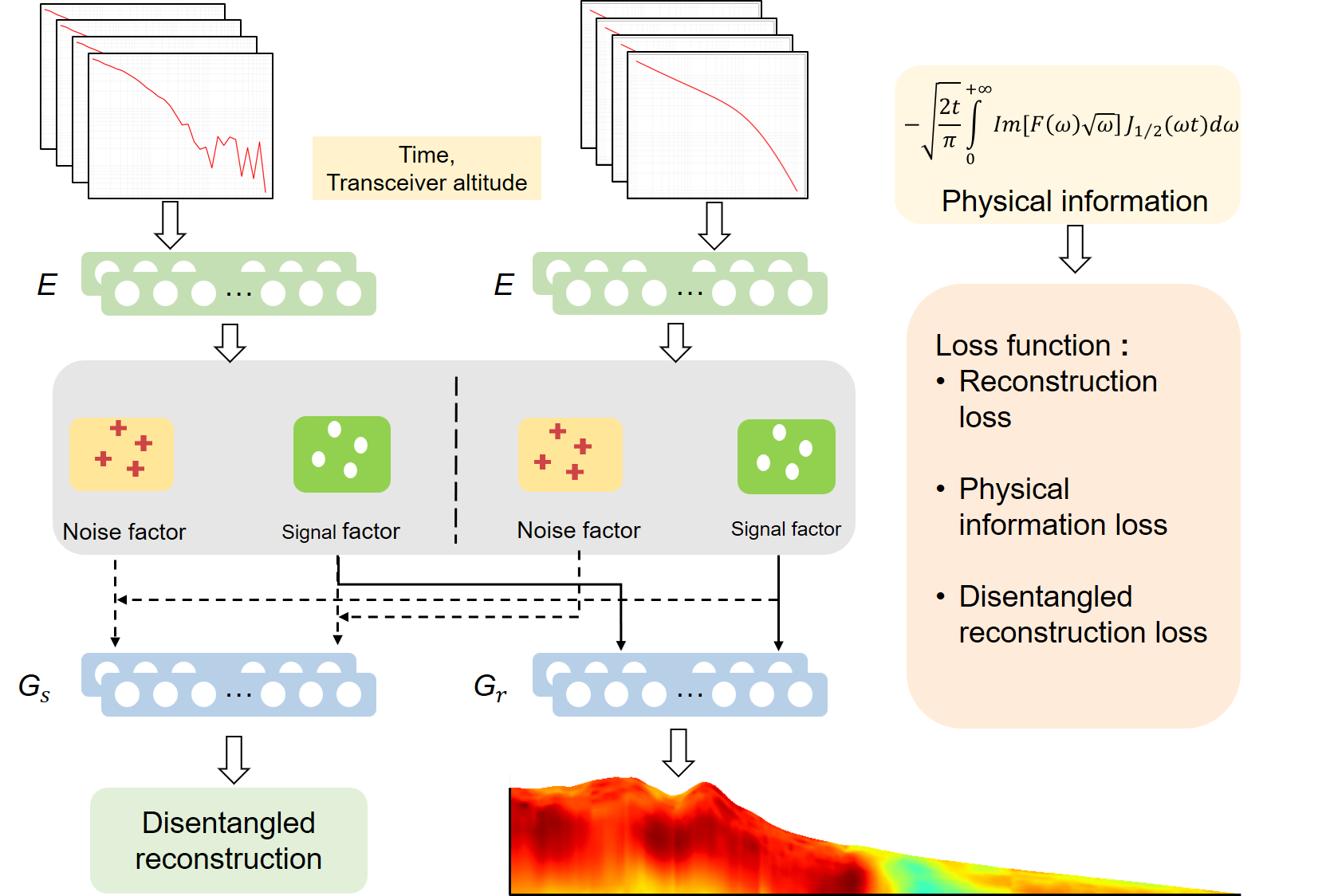
The network comprises an encoder $E$, an inversion decoder $G_{r}$, and a data decoder $G_{s}$. The encoder $E$ encodes the input data into signal and noise factors, while the inversion decoder $G_{r}$ decodes the signal factor to generate accurate inversion results. The data decoder $G_{s}$ decodes the combined signal and noise factors into the signal, ensuring the correctness of the disentangled representation.

Given the collected data $x$, the encoder $E$ encodes it into a pair of disentangled representations:

$$Z_{s},Z_{n}=E(x)$$ (1)

Here, $Z_{s}$ represents the signal factor, and $Z_{n}$ represents the noise factor. A mutual information upper bound estimator, CLUB [P. Cheng . (2020)], is employed to ensure that the distributions of $Z_{s}$ and $Z_{n}$ are fully separated, as the distributions of the signal and noise are entirely distinct.

During training, the encoder $E$ is used to encode both noisy signals $n$ and clean signals $s$. The network is expected to correctly obtain the disentangled representations $Z_{s}^{1},Z_{n}^{1}=E(n)$ and $Z_{s}^{2},Z_{n}^{2}=E(s)$. The signal factor representations, $Z_{s}^{1}$ and $Z_{s}^{2}$, should follow the same distribution, indicating they represent similar signal factors. In contrast, the noise factors differ, as the clean signal contains no noise. The noise factors are then swapped between the two representations, and the data decoder is employed to decode them. Decoding $(Z_{s}^{1},Z_{n}^{2})$ yields the clean signal, while decoding $(Z_{s}^{2},Z_{n}^{1})$ yields the noisy signal, demonstrating that the data has been fully disentangled. Finally, the inversion decoder $G_{r}$ is used to decode the signal factor and obtain the inversion result.

$$m=G_{r}(Z_{s}^{1})=G_{r}(Z_{s}^{2})$$ (2)

To address the challenge of data-driven networks relying on the completeness of training data, which necessitates that the training set adequately represent the variations in geophysical properties [S. Wu . (2024)], we incorporate physical information to guide and drive the network training process. This approach ensures that the model avoids biased interpretations of subsurface structures when applied to field observations. Given the resistivity model $m$, its forward response is:

$$s=F(m)$$ (3)

Here, $F$ represents the forward operator, and its computed response is as follows: Using the step waveform as an example, the current function is given by:

$$\begin{cases}I(t)=I_{0},t\leq 0\\ I(t)=0,t>0\end{cases}$$ (4)

The response result is given by:

$$f(t)=\frac{1}{2\pi}\int_{-\infty}^{+\infty}F(\omega)e^{i\omega t}d\omega$$ (5)

The term $e^{i\omega t}$ is the time-harmonic factor, where $\omega$ represents the angular frequency, and $F(\omega)$ is the frequency domain response. This can be further derived as [YIN . (2013)]:

$$f(t)=-\sqrt{\frac{2t}{\pi}}\int_{0}^{+\infty}\text{Im}\left[F(\omega)\sqrt{\omega}\right]J_{\frac{1}{2}}(\omega t)d\omega$$ (6)

Where $J_{\frac{1}{2}}(\omega t)$ is the half-integer order Bessel function. The response of an arbitrary emitted waveform is given by:

$$\frac{dB}{dt}=\frac{dI(t)}{dt}*f(t)$$ (7)

Where, $t$ represents the given time, and $I(t)$ is the emitted current. The forward operator is applied to the inversion result $m$ to obtain the physical constraint loss:

$$L_{physic}=||F(m)-s||^{2}$$ (8)

The overall loss function is:

$$L=L_{physic}+L_{clean}+L_{noise}+L_{rho}$$ (9)

$$L_{clean}=||G_{s}(Z_{s}^{2},Z_{n}^{2})-s||^{2}+||G_{s}(Z_{s}^{1},Z_{n}^{2})-s||^{2}$$ (10)

$$L_{noise}=||G_{s}(Z_{s}^{2},Z_{n}^{1})-n||^{2}+||G_{s}(Z_{s}^{1},Z_{n}^{1})-n||^{2}$$ (11)

$$L_{rho}=||m-m_{l}||^{2}$$ (12)

Where $m_{l}$ is the true resistivity model.

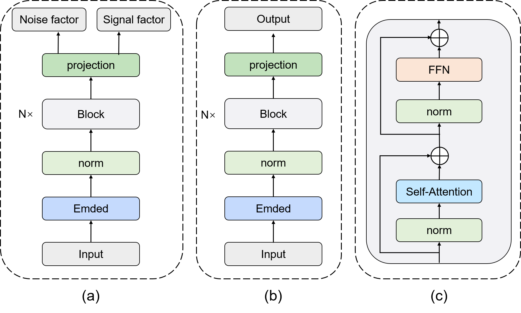
Since ATEM data exhibits strong temporal correlation, each data point is directly related to time. We also account for the influence of time on the data. Time embedding is applied during both encoding and decoding. Additionally, due to the varying heights of the transceiver, which also affect the data, we have embedded the heights of the transceiver into the network. Our focus is on the entire data processing pipeline rather than the network architecture itself. Therefore, the network structure follows the GPT-2 style [Lagler . (2013)], with the encoder depicted in Fig. 2(a). After embedding the input, it is processed by $N$ blocks, and the final output consists of a pair of decoded representations. The decoder, shown in Fig. 2(b), uses the decoupled representations output by the encoder as input to decode the target data. The block structure is illustrated in Fig. 2(c). The stackable block structure follows the general GPT design and consists of a self-attention module and a feedforward network (FFN) module.

Figure 2: (a) represents the architecture of the encoder E, (b) represents the architectures of the inversion decoder Gr and the data decoder Gs, and (c) shows the stacked block structure within the encoder and decoder.

3 Experiments

3.1 Dataset

We utilized the large resistivity model database (RMD) developed by [Asif . (2023)], which contains a variety of geologically plausible and geophysically resolvable subsurface structures. The database comprises approximately one million resistivity models, with resistivity values ranging from 1 to 2000 ohm-meters, consisting of 30 layers and a maximum depth of 500 meters. Each model adheres to physical constraints. RMD has been shown to improve performance and generalization while also enhancing the consistency and reliability of deep learning models [Y. Liu . (2024)].

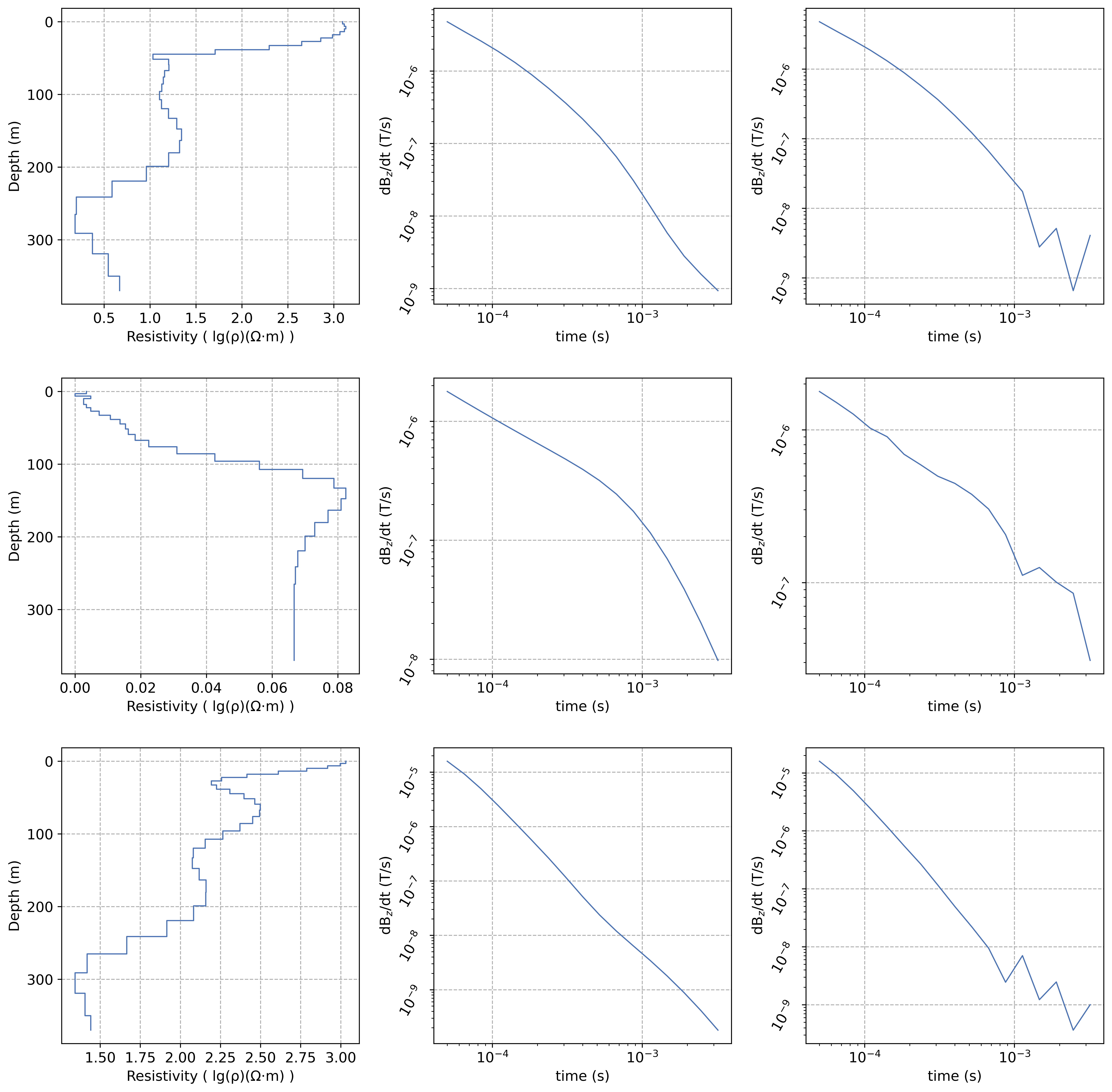
We conducted one-dimensional forward modeling [YIN . (2013)] on the entire model database to obtain the corresponding forward responses. The altitude of the transceiver varies uniformly within the range of 25–100 m above the surface. The ATEM system specifications, including transmit current and receiver configuration, align with those of the AeroTEM IV system described in [Bedrosian . (2014)]. Additionally, we introduced noise into the forward response data. Part of the noise was derived from actual field measurements, which includes motion-induced noise, nearby or moderately distant sferics noise, cultural and natural electromagnetic noise. As a type of incidental impulse noise, the amount of extraction of the nearby or moderately distant sferics noise was relatively small, while another part was Gaussian noise, as complex field noise distributions are often approximated by a Gaussian distribution [Chen . (2020)]. For the remaining noise, we selected a simulation method that has been shown to closely replicate actual noise [Auken . (2008)], which is defined as:

$$s_{n}=s+N(0,1)[STD^{2}+(\frac{n}{s})^{2}]^{\frac{1}{2}}s$$ (13)

Where, $s_{n}$ represents the obtained noisy signal, and $s$ is the forward theoretical data. $N(0,1)$ denotes the standard Gaussian distribution. STD is the uniform noise, and $n$ is the background noise contribution, which is defined as:

$$n=b{(\frac{t}{{10}^{-3}})}^{-\frac{1}{2}}$$ (14)

Where, $b$ is the noise level at 1 ms. It is typically taken between 1 nV/m² and 5 nV/m² [Auken . (2008)]. For some models, the forward data and the data after noise addition are shown in Fig. 3.

Figure 3: The 30-layer RMD model (on the left), forward response (in the middle), and the data after noise addition (on the right).

3.2 Train and Evaluation Metric

We randomly divided the obtained dataset into 10,000 validation sets and 10,000 test sets, with the remaining data designated as the training set. During training, the encoder and decoder each comprised 8 block stacks, with a batch size of 32. AdamW was used as the optimizer, and the learning rate was set to 0.0001. The model was trained for 200 epochs on an Nvidia A6000 GPU.

We use the Root Mean Square Percentage Error (RMSPE) to evaluate the accuracy of the inversion model and the signals generated by forward modeling based on this model.

$$RMSPE=\sqrt{\frac{1}{M}\sum_{j=1}^{M}(\frac{p_{j}^{r}-p_{j}^{t}}{p_{j}^{t}})^{2}\times 100\%}$$ (15)

Where $p_{j}^{r}$ and $p_{j}^{t}$ are the predicted values and the true values, respectively; M denotes the number of data points.

3.3 Inversion Performance on Test Dataset

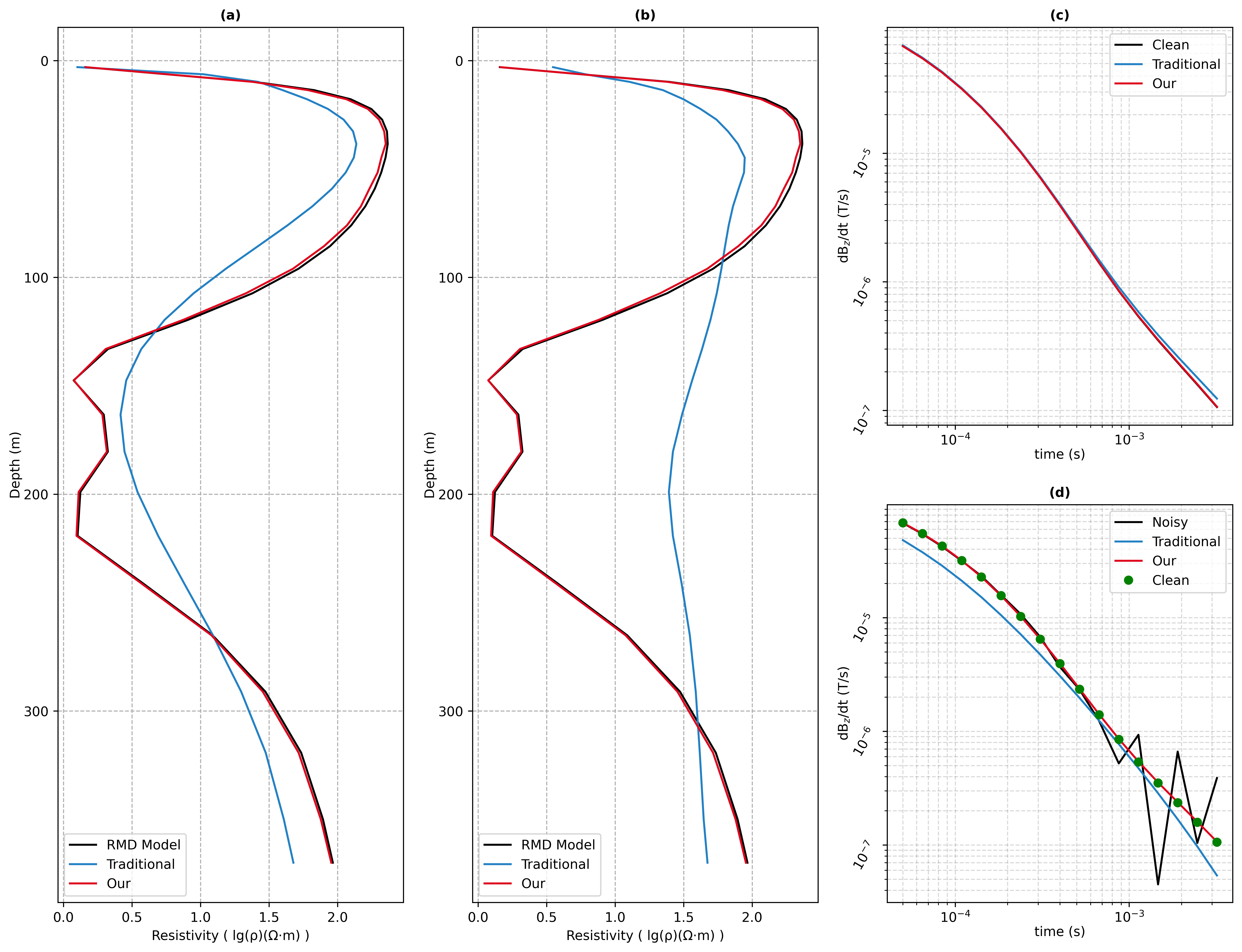
We first evaluated the performance of our method on the test set, comparing it with the traditional regularized inversion method [Yu . (2018)] that uses a combined regularization strategy, with conductivity-depth imaging (CDI) [Huang  Rudd (2008)] results serving as the initial model. As shown in Fig. 4 (a), when using clean signals for inversion, our method accurately fits the actual model, whereas the traditional approach provides a rough inversion and fails to capture the resistivity variation between 150m and 200m. We then performed forward modeling on the model, with the results shown in Fig. 4 (c). These results demonstrate that the forward signals from our method align better with the actual model’s forward signals, exhibiting smaller errors. Next, we tested the inversion capability on noisy signals. As shown in Fig. 4 (b), since our method decouples the noisy signal into signal and noise factors and uses the signal factor for inversion, it can still accurately decouple the same signal factor and obtain the same inversion result, even in the presence of noise. In contrast, the traditional method lacks adaptability to noisy signals, resulting in larger inversion errors. We performed forward modeling on the inversion results of the noisy signals, with the results shown in Fig. 4 (d). It is evident that our method still fits the actual model’s forward signals well, while the forward signals from the traditional method’s inverted model show significant deviation from the actual model’s forward signals.

Figure 4: (a) Inversion results using clean signals, (b) Inversion results using noisy signals, (c) Forward modeling response results using the inversion model from (a), (d) Forward modeling response results using the inversion model from (b).

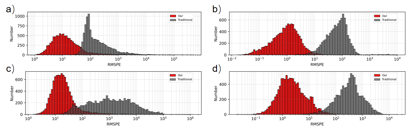
To evaluate the stability of the inversion, we analyzed the inversion results for the entire test set, as shown in Fig. 5. Fig. 5 (a) presents the RMSPE histogram of the inversion results for clean signals using both methods, compared to the true model. Our method demonstrates stable inversion results and accurately predicts the true model, while the traditional method exhibits a wider RMSPE distribution with some extreme values. This indicates that some traditional inversions failed to converge, leading to an increase in RMSPE values. Fig. 5 (b) shows the RMSPE histogram of the forward modeling response of the inversion result in (a) and clean signals. Although the forward modeling response closely matches the original signal values, the traditional method’s results still differ from the true model due to the non-uniqueness of ATEM inversion (multiple local minima). The inversion statistical histogram for noisy signals shows that our method maintains accurate inversion results even in the presence of noise, as it decouples the signal factor and performs stable inversion using this factor. In contrast, the traditional method is less robust to noise, resulting in significant deviation from the true model.

Figure 5: (a) RMSPE statistics of the inversion results for clean signals across the entire test set, (b) RMSPE statistics computed from the forward modeling response of the inversion results in (a) and the clean signals, (c) RMSPE statistics of the inversion results for noisy signals across the entire test set, (d) RMSPE statistics computed from the forward modeling response of the inversion results in (c) and the clean signals.

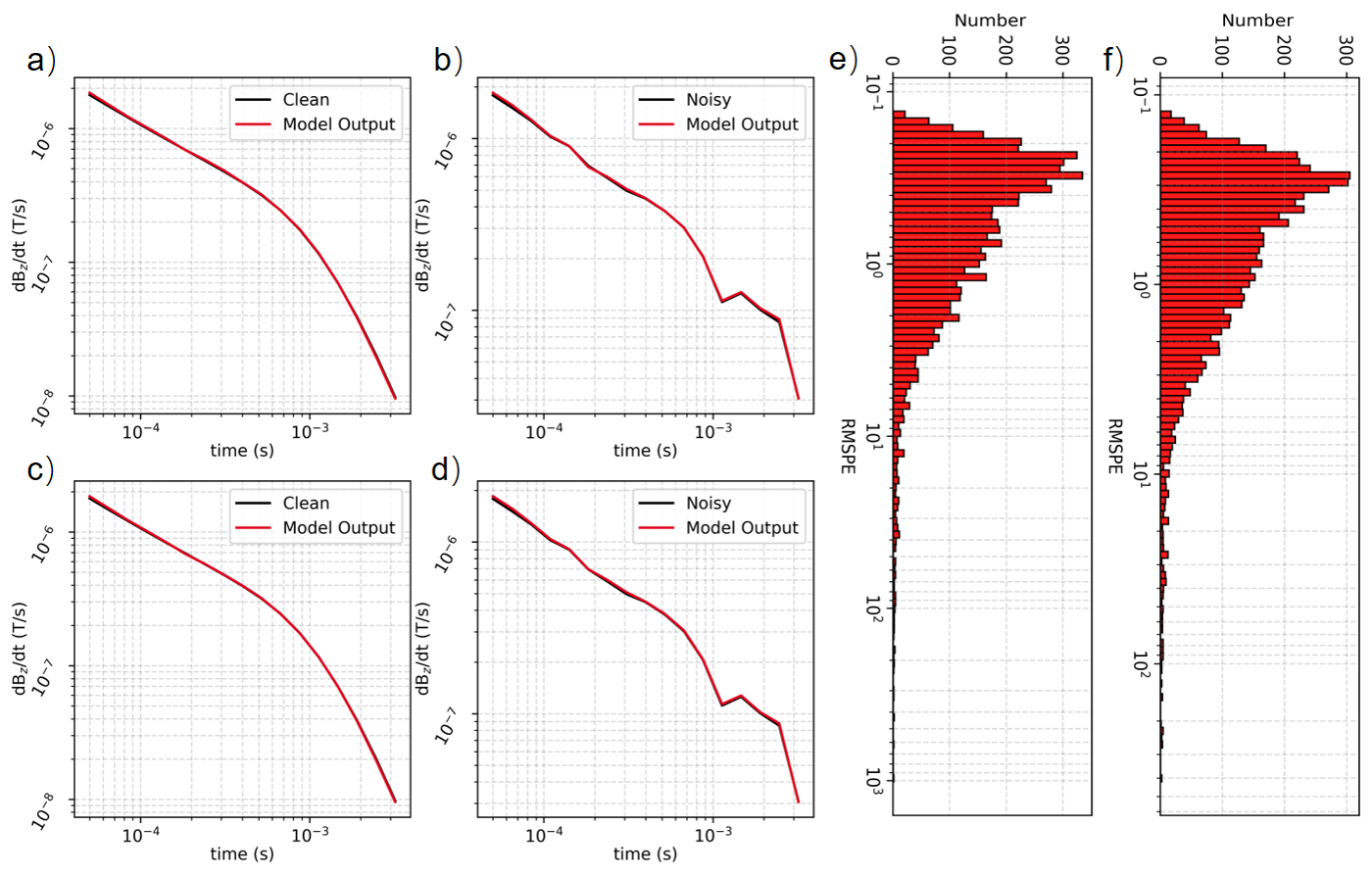
To ensure the network correctly decouples the data and that the encoder $E$ accurately encodes the data into signal and noise factors, we analyzed a set of clean and noisy signals and conducted statistical analysis on the test set, as shown in Fig. 6. The clean signal $s$ was decoupled into the signal factor $Z_{s}^{1}$ and the noise factor $Z_{n}^{1}$, while the noisy signal $n$ was decoupled into the signal factor $Z_{s}^{2}$ and the noise factor $Z_{n}^{2}$. By using various combinations of signal and noise factors, we were able to accurately reconstruct the corresponding signals, confirming that the network effectively decouples the data. We also performed a statistical analysis of the RMSPE histograms of the data decoded using $(Z_{s}^{1},Z_{n}^{1})$ and $(Z_{s}^{2},Z_{n}^{1})$, compared to the clean signal, as shown in Fig. 6 (e) and (f). These results highlight the network’s stable decoupling capability, demonstrating its ability to correctly encode the data into signal and noise factors.

Figure 6: The clean signal $s$ is decoupled into the signal factor $Z_{s}^{1}$ and the noise factor $Z_{n}^{1}$, while the noisy signal $n$ is decoupled into the signal factor $Z_{s}^{2}$ and the noise factor $Z_{n}^{2}$. (a) The clean signal decoded using $(Z_{s}^{1},Z_{n}^{1})$, (b) the noisy signal decoded using $(Z_{s}^{2},Z_{n}^{2})$, (c) the clean signal decoded using $(Z_{s}^{2},Z_{n}^{1})$, (d) the noisy signal decoded using $(Z_{s}^{1},Z_{n}^{2})$. (e) The RMSPE statistics of the clean signal decoded from $(Z_{s}^{1},Z_{n}^{1})$ on the test set, (f) The RMSPE statistics of the clean signal decoded from $(Z_{s}^{2},Z_{n}^{1})$ on the test set.

3.4 Field Data Application

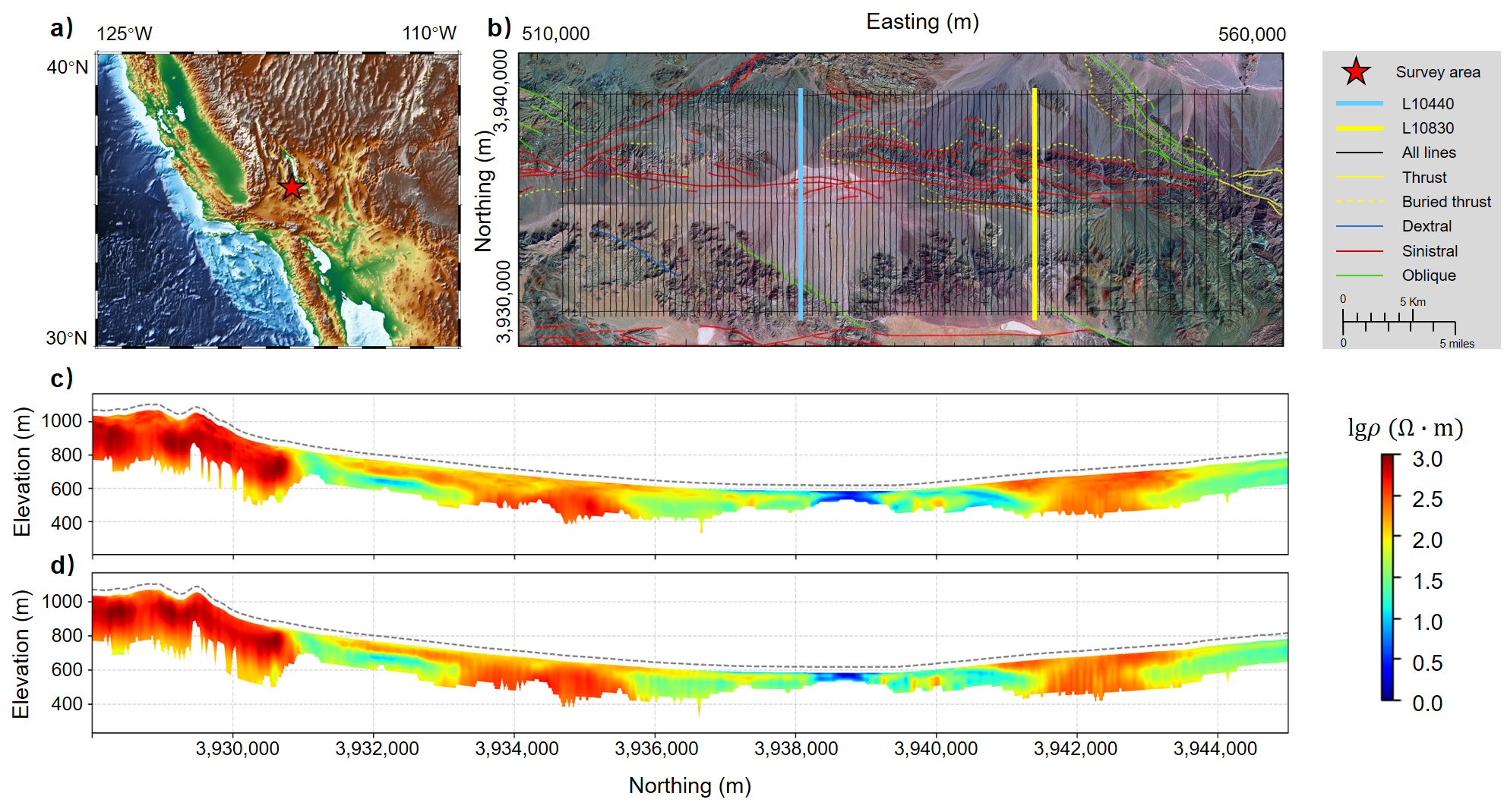
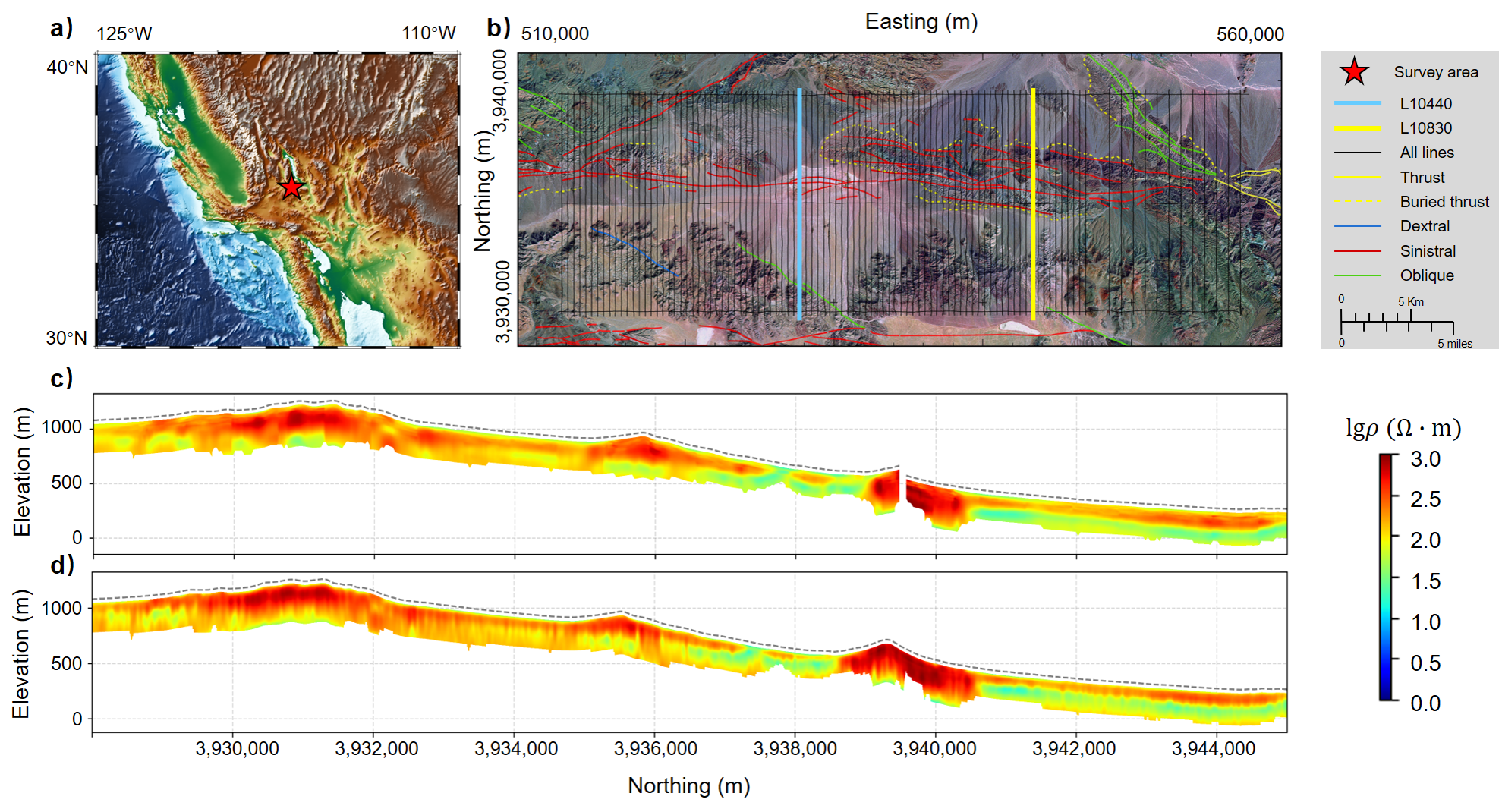
To demonstrate the applicability of the method, we tested the trained model on ATEM data collected by the United States Geological Survey (USGS) in the Leach Lake Basin at Fort Irwin, California, USA (Fig. 7 (a)). This survey area is a geologically complex, internally drained basin, characterized by numerous faults on both sides. The total length of the flight lines is 1,785.95 km, encompassing over 740,000 ATEM time series, as shown in Fig. 7 (b). Further details on the data can be found in the report by the USGS [Bedrosian . (2014)].

We present the inversion results for the L0440 survey line in Fig. 7. The USGS excluded data that could not be inverted due to severe noise interference and downsampled the remaining data by a factor of 10, resulting in 535 19-layer models, as shown in Fig. 7 (c). In contrast, our method successfully processed all 6,423 data points, yielding 6,423 30-layer models, as shown in Fig. 7 (d). Our method effectively reveals the subsurface electrical structure, aligning with the results obtained by the USGS. It clearly identifies faults, low-resistance areas, and high-resistance regions, demonstrating the accuracy and reliability of our inversion approach.

Figure 7: (a) Survey area, marked with a pentagram. (b) Distribution of flight lines (thin black lines). The thick blue line represents the L10440 survey line. (c) Resistivity profile of the L10440 survey line obtained by the USGS using traditional methods, consisting of 535 resistivity models. The black dashed line indicates the transceiver height. (d) Resistivity profile of the L10440 survey line obtained using our method, consisting of 6423 resistivity models.

We present the inversion results for the L0830 survey line in Fig. 8. The USGS excluded data significantly affected by environmental noise from their 515 19-layer inversion results, which led to gaps in the inversion profile and impacted the lateral resolution of the subsurface electrical structure. In contrast, our method processes all 6,412 data points without being influenced by noise, yielding 6,412 30-layer models, as shown in Fig. 8 (d). Our method provides subsurface electrical structures consistent with those obtained by the USGS, clearly identifying faults and other stratigraphic layers, while also revealing the gaps in the USGS inversion results, offering improved lateral resolution.

Figure 8: (a) Survey area, marked with a star. (b) Distribution of flight lines (thin black lines). The thick yellow line represents the L10830 survey line. (c) The resistivity profile of the L10830 survey line obtained by the USGS using traditional methods, consisting of 515 resistivity models. The black dashed line indicates the transmitter-receiver height. (d) The resistivity profile of the L10830 survey line obtained by our method, consisting of 6412 resistivity models.

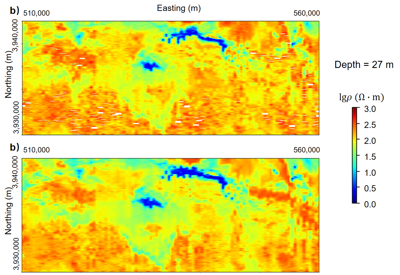
To validate the depth results obtained by the proposed method, we generated depth slices to analyze the lateral variations in resistivity. The depth slice at a depth of 27 meters is shown in Fig. 9. The results from our method are highly consistent with the USGS inversion results, clearly delineating the edge and extent of Leach Lake and the surrounding mountain contours. In contrast, the USGS inversion results excluded data affected by significant environmental noise, leading to gaps in the depth slice and affecting the lateral resolution of the subsurface electrical structure. Our method, however, processes all the data, providing a more accurate lateral representation.

Figure 9: Resistivity slices at a depth of 27 meters. (a) Inversion results obtained by USGS using traditional methods. (b) Inversion results obtained by our method.

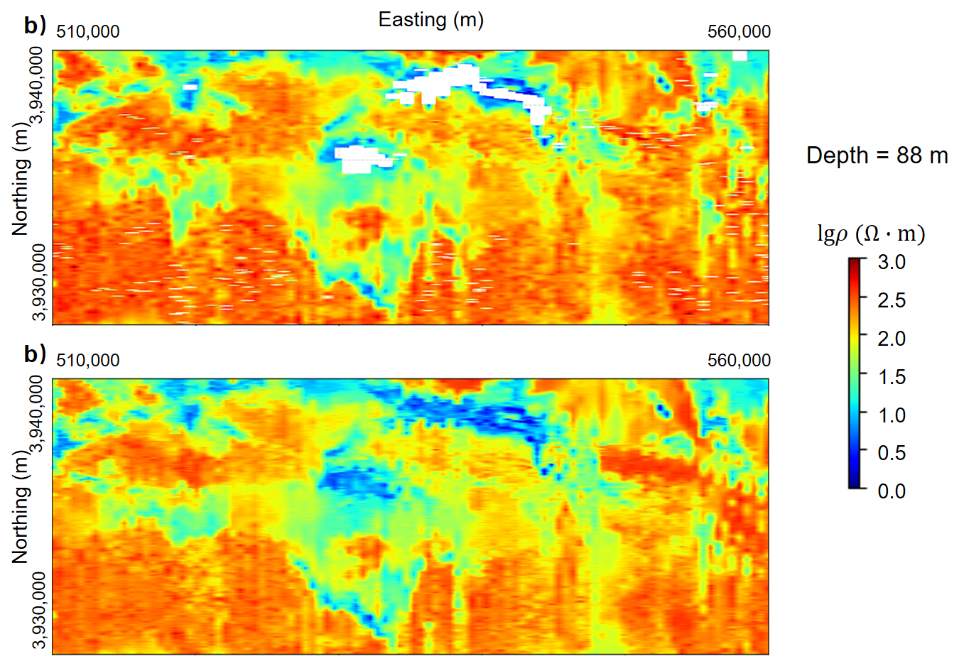
The depth slice at 88 meters, shown in Fig. 10, demonstrates that the results obtained by our method are consistent with the USGS inversion results, revealing well-defined lateral structures. This indicates that the inversion results produced by our proposed method are reliable at this depth and can be trusted for accurate interpretation.

Figure 10: Resistivity slices at a depth of 88 meters. (a) Inversion results obtained by USGS using traditional methods. (b) Inversion results obtained by our method.

The inversion results of field data from the Leach Lake Basin at Fort Irwin demonstrate that our method yields reliable results, accurately revealing the subsurface electrical structure. Additionally, it can directly handle noisy data, including data affected by significant environmental noise, which traditional methods struggle to process, providing enhanced lateral structural representations. Furthermore, the RMD used, with its well-structured and deep layers, enables the trained deep learning model to accurately reflect the actual subsurface electrical structure.

4 Conclusions

In this study, we propose a unified, interpretable deep learning inversion framework based on decoupled representation learning. The network effectively decouples noisy data into signal and noise factors, utilizing the signal factors for inversion. This approach integrates denoising and inversion processes for field data. By incorporating physical information as guidance and leveraging signal factors throughout the data processing pipeline, the network’s results are more reliable and interpretable. The inversion results from models trained on the RMD using field data demonstrate that our model can directly derive accurate subsurface electrical structures from noisy data. Moreover, it is capable of processing data affected by significant environmental noise, which traditional methods cannot handle, offering enhanced lateral structural representations.

Open Research

The airborne electromagnetic observations and resistivity models come from the U.S. Geological Survey report (http://dx.doi.org/10.3133/ofr20131024G).