DR-PETS: Learning-Based Control With Planning in Adversarial Environments

Abstract

Ensuring robustness against epistemic, possibly adversarial, perturbations is essential for reliable real-world decision-making. While the Probabilistic Ensembles with Trajectory Sampling (PETS) algorithm inherently handles uncertainty via ensemble-based probabilistic models, it lacks guarantees against structured adversarial or worst-case uncertainty distributions. To address this, we propose DR-PETS, a distributionally robust extension of PETS that certifies robustness against adversarial perturbations. We formalize uncertainty via a $p$-Wasserstein ambiguity set, enabling worst-case-aware planning through a min-max optimization framework. While PETS passively accounts for stochasticity, DR-PETS actively optimizes robustness via a tractable convex approximation integrated into PETS’ planning loop. Experiments on pendulum stabilization and cart-pole balancing show that DR-PETS certifies robustness against adversarial parameter perturbations, achieving consistent performance in worst-case scenarios where PETS deteriorates.

I INTRODUCTION

Deep reinforcement learning (RL) provides a powerful framework for sequential decision-making. However, deploying RL in practical settings demands robustness to epistemic uncertainty (e.g., adversarial perturbations or model mis-match) [1]. These uncertainties are often heterogeneous, non-stationary, or even adversarial, making robustness guarantees critical for safe deployment. While recent work has focused on robust RL methods that account for worst-case transitions [2], many state-of-the-art algorithms remain vulnerable to structured adversarial perturbations.

Model-based RL (MBRL) improves sample efficiency by learning an explicit environment model [3], enabling planning strategies like model predictive Control (MPC) [4] to simulate and optimize long-horizon decisions. Among MBRL methods, the probabilistic ensembles with trajectory sampling (PETS) algorithm [5] stands out: it combines probabilistic ensemble models with MPC to achieve high data efficiency and performance. However, PETS’ robustness stems implicitly from its ensemble-based uncertainty quantification, which assumes stochastic (not adversarial) deviations. This leaves it ill-equipped for scenarios where perturbations strategically exploit model inaccuracies [6].

Motivated by this, we propose DR-PETS, a distributionally robust version of PETS. In DR-PETS, planning is still achieved through MPC but, differently from PETS, the MPC cost is regularized and the regularizer arises from a suitable reformulation of the underlying control problem with ambiguity sets defined by the $p$-Wasserstein distance to capture epistemic uncertainties. Since this leads to an otherwise intractable problem, DR-PETS employs a tractable approximation, resulting in a regularized version of the original MPC cost. In what follows we briefly survey some closely related works on DR learning and MPC.

Related work

A common approach to handle uncertainty in RL is to consider worst-case transition models [7], often formalized via distributionally robust Markov decision processes (DR-MDPs) [8, 2], where ambiguity sets are modeled using the Wasserstein distance [9]. Building on this, [10] establishes a duality between robustness and regularization, a concept also leveraged in model-free DR RL, such as DR Q-learning [11], which recasts Q-values into a DR Bellman operator via strong duality. Convergence guarantees for Wasserstein-robust Q-learning in linear, time-invariant systems are provided in [12]. In [13], a robust RL framework for constrained MDP using optimal transport perturbations is proposed; however, unlike our method, it requires offline perturbation computation and application to training data. In DR-MPC, [14] formulates DR chance constraints and proposes a data-driven approach for value-at-risk under Wasserstein ambiguity, while [15] derives DR-MPC for conic moment-based ambiguity sets, assuming set shrinkage with more data. Finally, [16] proposes an ambiguity tube MPC for nonlinear stochastic systems with cost-to-go concavity.

Contributions

We propose DR-PETS, a DR extension of PETS that explicitly certifies robustness against adversarial perturbations. Our key contributions include: (i) integrating Wasserstein ambiguity sets into the MPC cost functional for worst-case-aware planning without perturbing training data [10, 13]; (ii) reformulating the intractable max-min problem via Wasserstein duality [17], yielding a convex maximization with a regularized cost; (iii) empirical validation on adversarial pendulum and cart-pole environments, demonstrating superior robustness over PETS; (iv) open-source implementation at https://tinyurl.com/595c76t6. Our work advances prior robust RL methods in three key ways: (1) unlike [13], which computes adversarial perturbations offline by corrupting training data and then deriving a policy, DR-PETS directly optimizes for a robust policy by maximizing a regularized reward function, eliminating the need for explicit perturbation injection; (2) avoids iterative forward simulations, unlike [hewing2019cautious], preserving PETS’ data efficiency; and (3) explicitly certifies robustness against adversarial perturbations, unlike PETS, which only accounts for stochastic uncertainty. While this work focuses on theoretical certification of robustness against adversarial perturbations in an unconstrained setting, it establishes a foundational framework for future research to rigorously integrate safety constraints; indeed, as showed in [13], the inclusion of safety constraints significantly amplifies the benefits of robust methods by reducing sensitivity to model perturbations. This is the objective of future researches.

II Preliminaries and problem setup

Sets are in calligraphic and vectors in bold. A random variable is denoted by $\mathbf{V}$ and its realization is $\mathbf{v}$. We denote the probability density function, or simply pdf, of $\mathbf{v}$ by $p(\mathbf{v})$. Whenever we take the integral involving a pdf we always assume that the integral exists. The expectation of a function $\mathbf{h}(\cdot)$ of $\mathbf{v}$ is $\mathbb{E}_{{p}}[\mathbf{h}(\mathbf{v})]:=\int\mathbf{h}(\mathbf{v})p(\mathbf{v})d\mathbf{\mathbf{v}}$, where the integration is over the support of $p(\mathbf{v})$. The conditional pdf of $\mathbf{v}_{1}$ with respect to $\mathbf{v}_{2}$ is $p\left(\mathbf{v}_{1}\mid\mathbf{v}_{2}\right)$. Countable sets are denoted by $w_{k_{1}:k_{n}}$, where $w_{k}$ is the generic set element, $k_{1}$ ($k_{n}$) is the index of the first (last) element and $k_{1}:k_{n}$ is the set of consecutive integers between (including) $k_{1}$ and $k_{n}$. We use $<\cdot,\cdot>$ as the inner product and $\bigotimes$ as the Cartesian product. Let $\mathcal{M}(\mathcal{B})$ represent set of distributions over a Borel set $\mathcal{B}$. Whenever it is clear from the context, a function $g(\cdot)$ is denoted by $g$. The norm is denoted by $\left\lVert\cdot\right\rVert$ and the dual norm by $\left\lVert\cdot\right\rVert_{*}$. The symbol $\approx$ denotes approximations.

II-A Probabilistic ensembles with trajectory sampling (PETS) algorithm

Consider a MDP [5] defined by the tuple $(\mathcal{X},\mathcal{U},f,r,\gamma)$, where $\mathcal{X}$ is the set of states and $\mathcal{U}$ is the set of actions, such that $f:\mathcal{X}\times\mathcal{U}\varrightarrow P(\mathcal{X})$ is the transition probability function where $P(\mathcal{X})$ denotes space of probability measures over $\mathcal{X}$, $r:\mathcal{X}\times\mathcal{U}\varrightarrow\mathbb{R}$ is the reward function, and $\gamma\in[0,1)$ is the discount factor. At time $t$, given state $\mathbf{x}_{t}\in\mathcal{X}\subseteq\mathbb{R}^{x}$, the agent applies action $\mathbf{u}_{t}\in\mathcal{U}\subseteq\mathbb{R}^{u}$, then the subsequent state $\mathbf{x}_{t+1}$ is determined by the conditional distribution $f(\mathbf{x}_{t+1}|\mathbf{x}_{t},\mathbf{u}_{t})$ i.e. $\mathbf{x}_{t+1}\sim f(\mathbf{x}_{t+1}|\mathbf{x}_{t},\mathbf{u}_{t}),\forall\mathbf{x}_{t+1}\in\mathcal{X}$, and $r(\mathbf{x}_{t},\mathbf{u}_{t})$ returns the immediate reward received when the MDP is in state $\mathbf{x}_{t}$ and $\mathbf{u}_{t}$ is applied. The results in [5] rely on the following:

Assumption 1

Given an MDP, $(\mathcal{X},\mathcal{U},f,r,\gamma)$ the transition probability function $f$ is unknown and reward $r$ is known.

Under Assumption 1, to estimate the transition probability function $f$, PETS collects a dataset $\mathcal{D}$ of $N\in\mathbb{Z}_{+}$ samples from the system, defined as $\{(\mathbf{x}_{t},\mathbf{u}_{t},\mathbf{x}_{t+1})\}_{t=0,1,\dots,N-1}$, where the actions are generated according to some criteria, e. g. randomly. Then an ensemble of $B\in\mathbb{Z}_{+}$ neural networks (NNs) can be trained on the collected dataset; formally, the $b$-th NN is modelled as a Gaussian distribution by $\hat{f}_{\theta_{b}}\sim\mathcal{N}(m_{\theta_{b}},\Sigma_{\theta_{b}})$, with $b=1,2,\dots,B$ and $\theta_{b}$ being the parameters of $b$-th NN. As in [5], given a system state $\mathbf{x}_{t}$ and an action $\mathbf{u}_{t}$, the output of the ensemble, i.e. the probability to reach the new expected state $\hat{\mathbf{x}}_{t+1}$, is the average over the NNs, i.e., $\hat{f}_{\theta}(\hat{\mathbf{x}}_{t+1}|\mathbf{x}_{t},\mathbf{u}_{t}):=\frac{1}{B}\sum\limits_{b=1}^{B}\hat{f}_{\theta_{b}}(\hat{\mathbf{x}}_{t+1}|\mathbf{x}_{t},\mathbf{u}_{t})$.

For planning and action selection, PETS uses an MPC-based policy. For a given current state $\hat{\mathbf{x}}_{t}$, system model $\hat{f}_{\theta}$ and a finite horizon $T\in\mathbb{Z}_{+}$, the RL planning through MPC maximizes the objective function

$$\begin{split}\mathcal{J}_{\hat{f}_{\theta}}(\hat{\mathbf{x}}_{t},\mathbf{u}_{t:t+T-1})=\mathbb{E}_{\hat{f}_{\theta}}\left[\sum\limits_{i=t}^{t+T-1}\gamma^{i-t}{r}(\hat{\mathbf{x}}_{i},\mathbf{u}_{i})|\hat{\mathbf{x}}_{t}\right],\end{split}$$ (1)

where we denote a simulated state by $\hat{\mathbf{x}}_{i}$, and for $i=t$ we initialize $\hat{\mathbf{x}}_{t}$ to $\mathbf{x}_{t}$ as system state. In (1) the expectation is over simulated future trajectories generated by $\hat{\mathbf{x}}_{i+1}\sim\hat{f}_{\theta}(\cdot|\hat{\mathbf{x}}_{i},\mathbf{u}_{i})$ given the initial state $\mathbf{x}_{t}$.

With this setting, PETS algorithm aims to find a finite sequence $\mathbf{u}_{t:t+T-1}^{*}:=\{\mathbf{u}_{t}^{*},\mathbf{u}_{t+1}^{*},\dots,\mathbf{u}_{t+T-1}^{*}\}$ such that

$$\begin{split}&\mathbf{u}_{t:t+T-1}^{\ast}\in\arg\max\limits_{\mathbf{u}_{t:t+T-1}}\mathcal{J}_{\hat{f}_{\theta}}(\hat{\mathbf{x}}_{t},\mathbf{u}_{t:t+T-1})\\ &s.t.\quad\mathbf{u}_{t:t+T-1}\in\mathcal{U}.\end{split}$$ (2)

II-B Distributionally robust MDPs

We introduce distributionally robust MDPs (DR-MDPs) following [10], where the unknown transition probability function $f$ is within an uncertainty set $\mathcal{F}$, i.e. $f\in\mathcal{F}$. As commonly assumed in the literature [13, 10], we let $\mathcal{F}$ to be $(\mathbf{x},\mathbf{u})$-rectangular i.e. $\mathcal{F}=\bigotimes_{(\mathbf{x},\mathbf{u})\in\mathcal{X}\times\mathcal{U}}\mathcal{F}_{\mathbf{x},\mathbf{u}}$ where $\mathcal{F}_{\mathbf{x},\mathbf{u}}$ is a set of transitions $f(\cdot|\mathbf{x},\mathbf{u})\in P(\mathcal{X})$ for a given state-action pair. Hence, $\mathcal{F}$ is a Borel set and we let any possible transition probability function $\tilde{f}$ be a random variable with support on $\mathcal{F}$, such that $\tilde{f}\sim\tilde{\mu}\in\mathcal{M}(\mathcal{F})$. Here, the class of the distributions $\mathcal{M}$ is the ambuiguity set each of which have support on $\mathcal{F}$.

Definition 1

($p$-Wasserstein distance [17]) Let $p\in[1,+\infty]$ and $(\mathcal{F},d)$ be a metric space, where $d:\mathcal{F}\times\mathcal{F}\rightarrow\mathbb{R}_{+}$ is a lower semicontinuous metric. The $p$-Wasserstein distance between $\hat{\mu},\tilde{\mu}\in\mathcal{M}$($\mathcal{F}$) is

$$\mathcal{W}_{p}(\tilde{\mu},\hat{\mu})=\inf\limits_{\psi\in\mathcal{Q}(\hat{\mu},\tilde{\mu})}\left(\int_{\mathcal{F}\times\mathcal{F}}d(\hat{f},\tilde{f})^{p}d\psi(\hat{f},\tilde{f})\right)^{\frac{1}{p}},$$ (3)

where $\mathcal{Q}(\hat{\mu},\tilde{\mu})$ is the set of distributions over $\mathcal{F}\times\mathcal{F}$ with marginals $\hat{\mu}$ and $\tilde{\mu}$.

Inspired by [10] and [18], we choose a $p$-Wasserstein ball $\Omega_{\epsilon}(\hat{\mu})$ as the ambiguity set over $\mathcal{F}$, centered in $\hat{\mu}$ and defined as

$$\Omega_{\epsilon}(\hat{\mu}):=\{\tilde{\mu}:\mathcal{W}_{p}(\tilde{\mu},\hat{\mu})\leq\epsilon\}$$ (4)

where $\epsilon>0$ is the radius of the ball, and $\hat{\mu}:=\frac{1}{B}\sum\limits_{b=1}^{B}\delta_{\hat{f}_{\theta_{b}}}$, with $\delta_{\hat{f}_{\theta_{b}}}$ being the Dirac distribution with full mass on $\hat{f}_{\theta_{b}}$.

II-C Problem statement

Following [10], we let the $p$-Wasserstein DR-MDP (WR-MDP) tuple as $(\mathcal{X},\mathcal{U},r,\mathcal{F},\Omega_{\epsilon}(\hat{\mu}))$, and we define corresponding DR formulation of (2) as:

Problem 1

Given a WR-MDP $(\mathcal{X},\mathcal{U},r,\mathcal{F},\Omega_{\epsilon}(\hat{\mu}))$, find the sequence of control inputs $\mathbf{u}_{t:t+T-1}^{*}:=\{\mathbf{u}_{t}^{*},\mathbf{u}_{t+1}^{*},\dots,\mathbf{u}_{t+T-1}^{*}\}$ such that,

$$\mathbf{u}_{t:t+T-1}^{*}\in\arg\max\limits_{\mathbf{u}_{t:t+T-1}}\inf_{\tilde{\mu}\in\Omega_{\epsilon}(\hat{\mu})}\mathbb{E}_{\tilde{f}\sim\tilde{\mu}}\left[\mathcal{J}_{\tilde{f}}(\mathbf{x}_{t},\mathbf{u}_{t:t+T-1})\right]$$

$$s.t.\quad{\mathbf{u}_{t},\mathbf{u}_{t+1},\dots,\mathbf{u}_{t+T-1}}\in\mathcal{U},$$ (5)

where $\mathcal{J}_{\tilde{f}}(\mathbf{x}_{t},\mathbf{u}_{t:t+T-1})$ is defined as in (1).

By evaluating the infimum over the ambiguity set $\Omega_{\epsilon}(\hat{\mu})$ in (1) we consider a worst-case scenario for the objective function in (1), and this corresponds to a robust formulation of (2). To lighten the notation, for any given transition probability function $\tilde{f}$ and time sequence $t+i:t+T-1$ starting from current time $t+i$, we denote $\mathcal{J}_{\tilde{f}}(\mathbf{x}_{t+i},\mathbf{u}_{t+i:t+T-1})$ with $\mathcal{J}_{t+i}(\tilde{f})$. In the subsequent analysis we make the following assumption:

Assumption 2

Consider Problem 1 with $\Omega_{\epsilon}(\hat{\mu})$ defined in (4). The radius of the ball, $\epsilon$, is such that $\mathcal{J}_{t}(\bar{f})\approx\mathcal{J}_{t}(\hat{f}_{\theta_{b}})+\left<\nabla_{\hat{f}_{\theta_{b}}}\mathcal{J}_{t}(\hat{f}_{\theta_{b}}),v_{b}\right>,$ for all $\bar{f}\in\Omega_{\epsilon}(\hat{\mu})$.

Remark 1

Assumption 2 is standard in the literature on DR-RL (see e.g. [10], [13] and [19]). Intuitively, it implies that $\epsilon$ is sufficiently small, i.e., within the feasibility domain of Problem 1 a first order approximation for the cost holds.

Authors in [18] and [13] showed that the objective function in Problem 1 is intractable. Our main objective is to derive a tractable reformulation of cost function in (1). We do this by leveraging the strong duality of (1), as established in [17],

$$\inf_{\tilde{\mu}\in\Omega_{\epsilon}(\hat{\mu})}\mathbb{E}_{\tilde{f}\sim\tilde{\mu}}\mathcal{J}_{t}(\tilde{f})$$

$$=\inf_{\tilde{\mu}}\sup\limits_{\lambda\geq 0}\Biggl{\{}\mathbb{E}_{\tilde{f}\sim\tilde{\mu}}\left[\mathcal{J}_{t}(\tilde{f})\right]$$ (6)

$$\qquad\qquad\qquad-\lambda\Biggl{(}\epsilon^{p}-\frac{1}{B}\sum\limits_{b=1}^{B}\mathbb{E}_{{f_{b}}\sim{\mu_{b}}}\left[d(f_{b},\hat{f}_{\theta_{b}})^{p}\right]\Biggr{)}\Biggr{\}}$$

$$=\sup\limits_{\lambda\geq 0}\Biggl{\{}\frac{1}{B}\sum\limits_{b=1}^{B}\inf_{\tilde{f}_{b}}\left\{\mathcal{J}_{t}(\tilde{f}_{b})+\lambda(d(\tilde{f}_{b},\hat{f}_{\theta_{b}})^{p})\right\}-\lambda\epsilon^{p}\Biggr{\}}.$$

Our approach aligns with the DR framework proposed in [11], although developed for a finite discrete state space. Indeed, for our framework of a continuous state space we use of an ensemble of neural networks to model the transition dynamics $f$ and the subsequent derivation of a regularized reward function through a Wasserstein ambiguity set.

III Main results

To develop the DR-PETS algorithm we need a tractable reformulation of (1) for which we employ the last equality in (II-C). In fact, in the following Theorem we show that (II-C) is formed of two terms: the empirical estimate of the performance index over the ensemble and a regularizer.

Theorem III.1

Let Assumption 2 hold. Then:

$$\sup_{\lambda\geq 0}\biggr{\{}\frac{1}{B}\sum\limits_{b=1}^{B}\inf_{\tilde{f}_{b}}\bigr{[}\mathcal{J}_{t}(\tilde{f}_{b})+\lambda(d(\tilde{f}_{b},\hat{f}_{\theta_{b}})^{p})\bigl{]}-\lambda\epsilon^{p}\biggl{\}}$$

$$=\frac{1}{B}\sum\limits_{b=1}^{B}\mathcal{J}_{t}(\hat{f}_{\theta_{b}})-\epsilon\biggr{(}\frac{1}{B}\sum\limits_{b=1}^{B}\left\lVert\nabla_{\hat{f}_{\theta_{b}}}\mathcal{J}_{t}(\hat{f}_{\theta_{b}})\right\rVert_{\ast}^{\frac{p}{p-1}}\biggl{)}^{\frac{p-1}{p}}.$$ (7)

Proof:

Motivated by the approach of [19] and relying on Assumption 2 we can write the last equality in (II-C) as

$$\sup_{\lambda\geq 0}\biggr{\{}\frac{1}{B}\sum\limits_{b=1}^{B}\inf_{\tilde{f}_{b}}\left[\mathcal{J}_{t}(\tilde{f}_{b})+\lambda(d(\tilde{f}_{b},\hat{f}_{\theta_{b}})^{p})\right]-\lambda\epsilon^{p}\biggl{\}}$$

$$\approx\frac{1}{B}\sum\limits_{b=1}^{B}\mathcal{J}_{t}(\hat{f}_{\theta_{b}})+\sup_{\lambda\geq 0}\biggr{\{}\frac{1}{B}\sum\limits_{b=1}^{B}\inf_{v_{b}}\Bigl{[}\left<\nabla_{\hat{f}_{\theta_{b}}}\mathcal{J}_{t}(\hat{f}_{\theta_{b}}),v_{b}\right>$$

$$\qquad\qquad+\lambda(\left\lVert v_{b}\right\rVert^{p})\Bigr{]}-\lambda\epsilon^{p}\biggl{\}}.$$ (8)

We begin our proof by solving the inner minimization problem in (III); we define $j(v_{b})$ as

$$\inf_{v_{b}}j(v_{b}):=\inf\limits_{v_{b}}\left\{\left<\nabla_{\hat{f}_{\theta_{b}}}\mathcal{J}_{t}(\hat{f}_{\theta_{b}}),v_{b}\right>+\lambda\left\lVert v_{b}\right\rVert^{p}\right\},$$ (9)

where we introduce the auxiliary variable $\delta_{b}$, such that $\left\lVert v_{b}\right\rVert\geq\delta_{b}$, obtaining

$$\begin{split}&\inf\limits_{v_{b},\delta_{b}}\left\{\left<\nabla_{\hat{f}_{\theta_{b}}}\mathcal{J}_{t}(\hat{f}_{\theta_{b}}),v_{b}\right>+\lambda\delta_{b}^{p}\mid\left\lVert v_{b}\right\rVert\leq\delta_{b}\right\}\\ &=\inf_{v_{b},\delta_{b}}\left\{h(v_{b},\delta_{b})\mid\left\lVert v_{b}\right\rVert\leq\delta_{b}\right\}.\end{split}$$ (10)

First, note that for any $v_{b}$, $j(v_{b})\leq h(v_{b},\delta_{b})$ for all feasible $\delta_{b}$ in (10). This implies $j(v_{b})\leq\inf_{\delta_{b}}\left\{h(v_{b},\delta_{b}\mid\left\lVert v_{b}\right\rVert\leq\delta_{b})\right\}$, and by minimizing both sides w.r.t $v_{b}$ we see that

$$\inf_{v_{b}}j(v_{b})\leq\inf_{v_{b},\delta_{b}}\left\{h(v_{b},\delta_{b})\mid\left\lVert v_{b}\right\rVert\leq\delta_{b}\right\}.$$

Let $\delta_{b}^{*}=\left\lVert v_{b}^{*}\right\rVert$, where $v_{b}^{*}$ is the optimal solution to (9), and note that $(v_{b}^{*},\delta_{b}^{*})$ is a feasible solution to (10) such that $h(v_{b}^{*},\delta_{b}^{*})=j(v_{b}^{*})$. Therefore, we can derive the optimal solution of (9) by finding the optimal solution of (10):

$$\inf\limits_{v_{b},\delta_{b}}\left\{\left<\nabla_{\hat{f}_{\theta_{b}}}\mathcal{J}_{t}(\hat{f}_{\theta_{b}}),v_{b}\right>+\lambda\delta_{b}^{p}\mid\left\lVert v_{b}\right\rVert\leq\delta_{b}\right\}$$

$$=\inf\limits_{\delta_{b}\geq 0}\left\{\inf\limits_{v_{b}}\left\{\left<\nabla_{\hat{f}_{\theta_{b}}}\mathcal{J}_{t}(\hat{f}_{\theta_{b}}),v_{b}\right>+\lambda\delta_{b}^{p}\mid\left\lVert v_{b}\right\rVert\leq\delta_{b}\right\}\right\}$$

$$=\inf\limits_{\delta_{b}\geq 0}\left\{\lambda\delta_{b}^{p}+\inf\limits_{\left\lVert v_{b}\right\rVert\leq\delta_{b}}\left\{\left<\nabla_{\hat{f}_{\theta_{b}}}\mathcal{J}_{t}(\hat{f}_{\theta_{b}}),v_{b}\right>\right\}\right\}$$

$$=\inf\limits_{\delta_{b}\geq 0}\left\{\lambda\delta_{b}^{p}-\delta_{b}\left\lVert\nabla_{\hat{f}_{\theta_{b}}}\mathcal{J}_{t}(\hat{f}_{\theta_{b}})\right\rVert_{*}\right\},$$ (11)

where the last step comes from the definition of the dual norm $\left\lVert\cdot\right\rVert_{*}$. The minimization over $\delta_{b}$ in (III) is dependent on $\lambda$ and the value $\delta_{b}^{*}(\lambda)$ that achieves the minimum can be obtained by exploiting the convexity of (III) in $\delta_{b}$. To obtain $\delta_{b}^{*}(\lambda)$ we set the derivative of $\lambda\delta_{b}^{p}-\delta_{b}\left\lVert\nabla_{\hat{f}_{\theta_{b}}}\mathcal{J}_{t}(\hat{f}_{\theta_{b}})\right\rVert_{*}$ with respect to $\delta_{b}$ equal to zero, which leads to

$$\delta_{b}^{*}(\lambda)=\left(\frac{\left\lVert\nabla_{\hat{f}_{\theta_{b}}}\mathcal{J}_{t}(\hat{f}_{\theta_{b}})\right\rVert_{*}}{p\lambda}\right)^{\frac{1}{p-1}}.$$

By plugging $\delta_{b}^{*}(\lambda)$ in (III) we obtain a solution to the inner minimization in (III):

$$\begin{split}&\inf\limits_{v_{b}}\left[\left<\nabla_{\hat{f}_{\theta_{b}}}\mathcal{J}_{t}(\hat{f}_{\theta_{b}}),v_{b}\right>+\lambda\left\lVert v_{b}\right\rVert^{p}\right]\\ &=\lambda(\delta_{b}^{*}(\lambda))^{p}-\delta_{b}^{*}(\lambda)\left\lVert\nabla_{\hat{f}_{\theta_{b}}}\mathcal{J}_{t}(\hat{f}_{\theta_{b}})\right\rVert_{*}\\ &=\frac{(1-p)\left\lVert\nabla_{\hat{f}_{\theta_{b}}}\mathcal{J}_{t}(\hat{f}_{\theta_{b}})\right\rVert_{*}^{\frac{p}{p-1}}}{p^{\frac{p}{p-1}}\lambda^{\frac{1}{p-1}}}.\end{split}$$ (12)

We can now solve the outer maximization in (III) by using (12) which leads to

$$\sup_{\lambda\geq 0}\biggr{\{}\frac{1}{B}\sum\limits_{b=1}^{B}\inf_{v_{b}}\left[\left<\nabla_{\hat{f}_{\theta_{b}}}\mathcal{J}_{t}(\hat{f}_{\theta_{b}}),v_{b}\right>+\lambda(\left\lVert v_{b}\right\rVert^{p})\right]-\lambda\epsilon^{p}\biggl{\}}$$

$$=\sup_{\lambda\geq 0}\left\{\frac{(1-p)\left(\frac{1}{B}\sum_{b=1}^{B}\left\lVert\nabla_{\hat{f}_{\theta_{b}}}\mathcal{J}_{t}(\hat{f}_{\theta_{b}})\right\rVert_{*}^{\frac{p}{p-1}}\right)}{p^{\frac{p}{p-1}}\lambda^{\frac{1}{p-1}}}-\lambda\epsilon^{p}\right\}.$$ (13)

Note that (III) is a maximization of a concave function in $\lambda$: the solution can be obtained by setting the derivative of (III) w.r.t. $\lambda$ equal to zero:

$$\frac{\mathrm{d}}{\mathrm{d}\lambda}\left(\frac{(1-p)\left(\frac{1}{B}\sum_{b=1}^{B}\left\lVert\nabla_{\hat{f}_{\theta_{b}}}\mathcal{J}_{t}(\hat{f}_{\theta_{b}})\right\rVert_{*}^{\frac{p}{p-1}}\right)}{p^{\frac{p}{p-1}}\lambda^{\frac{1}{p-1}}}-\lambda\epsilon^{p}\right)$$

$$=\frac{\left(\frac{1}{B}\sum_{b=1}^{B}\left\lVert\nabla_{\hat{f}_{\theta_{b}}}\mathcal{J}_{t}(\hat{f}_{\theta_{b}})\right\rVert_{*}^{\frac{p}{p-1}}\right)}{p^{\frac{p}{p-1}}\lambda^{\frac{p}{p-1}}}-\epsilon^{p}.$$ (14)

Setting (III) equal to zero and solving for $\lambda$ gives,

$$\lambda^{*}=\frac{\left(\frac{1}{B}\sum_{b=1}^{B}\left\lVert\nabla_{\hat{f}_{\theta_{b}}}\mathcal{J}_{t}(\hat{f}_{\theta_{b}})\right\rVert_{*}^{\frac{p}{p-1}}\right)^{\frac{p-1}{p}}}{p\epsilon^{p-1}}.$$

By plugging $\lambda^{*}$ into (III) we have

$$\begin{split}&\frac{(1-p)\left(\frac{1}{B}\sum_{b=1}^{B}\left\lVert\nabla_{\hat{f}_{\theta_{b}}}\mathcal{J}_{t}(\hat{f}_{\theta_{b}})\right\rVert_{*}^{\frac{p}{p-1}}\right)}{p^{\frac{p}{p-1}}\lambda^{*\frac{1}{p-1}}}-\lambda^{*}\epsilon^{p}\\ &=-\epsilon\left(\sum_{b=1}^{B}\left\lVert\nabla_{\hat{f}_{\theta_{b}}}\mathcal{J}_{t}(\hat{f}_{\theta_{b}})\right\rVert_{*}^{\frac{p}{p-1}}\right)^{\frac{p-1}{p}}.\end{split}$$ (15)

Finally, combining (15) with (III) we arrive at (III.1) as the closed form solution.∎

As in PETS algorithm, we compute the expectation over the estimated state trajectory in (1) using a particle-based propagation, i.e., propagating $Q\in\mathbb{Z}_{+}$ particles from initial state $\hat{\mathbf{x}}^{\text{q}}_{t}=\mathbf{x}_{t}$ at time $t$, where $\text{q}=1,2,\dots,Q$. Each particle is propagated using $\hat{\mathbf{x}}^{\text{q}}_{t+1}\sim\hat{f}_{\theta_{b}}$. Furthermore, as in PETS, we use cross entropy method (CEM) [20] to select actions, which iteratively samples $M\in\mathbb{Z}_{+}$ action sequences $\{\mathbf{u}_{t:t+T-1}^{i}\}_{i=1,2,\dots,M}$ from a candidate distribution $\mathbf{CEM}(\cdot):=\mathcal{N}(\varphi_{\mathbf{u}},\Sigma_{\mathbf{u}})$. Actions sampled from the candidate distribution are evaluated using (III.1), and parameters $\varphi_{\mathbf{u}}$ and $\Sigma_{\mathbf{u}}$ are updated iteratively based on best action sequence among $M$ samples.

By exploiting the B-NNs ensemble and letting $p=2$ we develop a simplified version of (III.1) that we use in our DR-PETS algorithm that is reported in the following result.

Theorem III.2

Given the problem in (1), the optimization objective can be reformulated as,

$$\begin{split}&\max_{\mathbf{u}_{t:t+T-1}}\biggr{\{}\frac{1}{B}\sum\limits_{b=1}^{B}\mathbb{E}_{\hat{f}_{\theta_{b}}}\biggr{[}\sum\limits_{i=t}^{t+T-1}\gamma^{i-t}r(\hat{\mathbf{x}}_{i},\mathbf{u}_{i})\biggl{]}\\ &-\epsilon\biggr{(}\frac{1}{B}\sum\limits_{b=1}^{B}\bigg{\|}\sum\limits_{k=1}^{T-1}\gamma^{k}\mathbb{E}_{\hat{\mathbf{x}}_{t+1:t+k}\sim\hat{f}_{\theta_{b}}}\\ &\biggr{[}\nabla_{\hat{f}_{\theta_{b}}}\ln(\hat{f}_{\theta_{b}}(\hat{\mathbf{x}}_{t+k}|\hat{\mathbf{x}}_{t+k-1},\mathbf{u}_{t+k-1}))\\ &\sum\limits_{i=t+k}^{t+T-1}\mathbb{E}_{\hat{\mathbf{x}}_{i+1}\sim\hat{f}_{\theta_{b}}}\bigr{[}\gamma^{i-t-k}r(\hat{\mathbf{x}}_{i},\mathbf{u}_{i})\bigl{]}\biggl{]}\bigg{\|}^{2}\biggl{)}^{\frac{1}{2}}\biggl{\}}\\ &s.t.\quad{\mathbf{u}_{t},\mathbf{u}_{t+1},\dots,\mathbf{u}_{t+T-1}}\in\mathcal{U}.\end{split}$$ (16)

Proof:

Considering Theorem III.1, when $p=2$, the l.h.s. of (III.1) can be rewritten as,

$$\begin{split}&\frac{1}{B}\sum\limits_{b=1}^{B}\mathcal{J}_{t}(\hat{f}_{\theta_{b}})-\epsilon\left(\frac{1}{B}\sum\limits_{b=1}^{B}\left\lVert\nabla_{\hat{f}_{\theta_{b}}}\mathcal{J}_{t}(\hat{f}_{\theta_{b}})\right\rVert^{2}\right)^{\frac{1}{2}}.\end{split}$$ (17)

Now, considering the horizon $T$, during the planning we sample $M$ possibly different sequences of actions, i.e., $\{\mathbf{u}_{t:t+T-1}^{k}\}_{k=1,2,\dots,M}$. Thus, the expectation in the first part of (17) is only w.r.t. $\hat{f}_{\theta_{b}}$, and it can be approximated by propagating $Q$ particles for each $k$. Next, we simplify the gradient term $\nabla_{\hat{f}_{\theta_{b}}}\mathcal{J}_{t}(\hat{f}_{\theta_{b}})$ in (17) by unrolling it over time horizon $T$. We use $\hat{\mathbf{x}}$ to emphasize that the state is predicted using the learned model. For brevity consider $\mathcal{J}_{t}=\mathcal{J}_{t}(\hat{f}_{\theta_{b}})$.

$$\begin{split}&\nabla_{\hat{f}_{\theta_{b}}}\mathcal{J}_{t}=\nabla_{\hat{f}_{\theta_{b}}}\biggr{[}\sum\limits_{i=t}^{t+T-1}\mathbb{E}_{\hat{f}_{\theta_{b}}}\bigr{[}\gamma^{i-t}r(\hat{\mathbf{x}}_{i},\mathbf{u}_{i})\bigl{]}\biggl{]}\\ &=\gamma\int\nabla_{\hat{f}_{\theta_{b}}}\biggr{(}\hat{f}_{\theta_{b}}(\hat{\mathbf{x}}_{t+1}|\hat{\mathbf{x}}_{t},\mathbf{u}_{t})\mathcal{J}_{t+1}\biggl{)}d{\hat{\mathbf{x}}_{t+1}}\\ &=\phi(\hat{\mathbf{x}}_{t},\mathbf{u}_{t})+\gamma\int\hat{f}_{\theta_{b}}(\hat{\mathbf{x}}_{t+1}|\hat{\mathbf{x}}_{t},\mathbf{u}_{t})\nabla_{\hat{f}_{\theta_{b}}}\left(\mathcal{J}_{t}\right)d{\hat{\mathbf{x}}_{t+1}},\end{split}$$ (18)

where $\phi(\hat{\mathbf{x}}_{t},\mathbf{u}_{t})=\gamma\int\nabla_{\hat{f}_{\theta_{b}}}\bigr{(}\hat{f}_{\theta_{b}}(\hat{\mathbf{x}}_{t+1}|\hat{\mathbf{x}}_{t},\mathbf{u}_{t})\bigl{)}\mathcal{J}_{t}d{\hat{\mathbf{x}}_{t+1}}.$

Continuing the unrolling of (18) with $\hat{f}_{\theta_{b}}(\hat{\mathbf{x}}_{t+i})=\hat{f}_{\theta_{b}}(\hat{\mathbf{x}}_{t+i}|\hat{\mathbf{x}}_{t+i-1},\mathbf{u}_{t+i-1})$ we have:

$$\nabla_{\hat{f}_{\theta_{b}}}\mathcal{J}_{t}=\phi(\hat{\mathbf{x}}_{t},\mathbf{u}_{t})+\gamma\int\hat{f}_{\theta_{b}}(\hat{\mathbf{x}}_{t+1})\nabla_{\hat{f}_{\theta_{b}}}\mathcal{J}_{t+1}d\hat{\mathbf{x}}_{t+1}$$

$$=\phi(\hat{\mathbf{x}}_{t},\mathbf{u}_{t})+\gamma\int\hat{f}_{\theta_{b}}(\hat{\mathbf{x}}_{t+1})\phi(\hat{\mathbf{x}}_{t+1},\mathbf{u}_{t+1})d\hat{\mathbf{x}}_{t+1}$$

$$+\gamma^{2}\int\hat{f}_{\theta_{b}}(\hat{\mathbf{x}}_{t+1})\int\hat{f}_{\theta_{b}}(\hat{\mathbf{x}}_{t+2})\phi(\hat{\mathbf{x}}_{t+2},\mathbf{u}_{t+2})d\hat{\mathbf{x}}_{t+2}d\hat{\mathbf{x}}_{t+1}+$$

$$\dots+\gamma^{T-1}\int\hat{f}_{\theta_{b}}(\hat{\mathbf{x}}_{t+1})\dots$$

$$\int\hat{f}_{\theta_{b}}(\hat{\mathbf{x}}_{t+T-1})\nabla_{\hat{f}_{\theta_{b}}}\mathcal{J}_{t+T-1}d\hat{\mathbf{x}}_{t+T-1:t+1}.$$ (19)

Note that, $\nabla_{\hat{f}_{\theta_{b}}}\mathcal{J}_{t+T-1}=\nabla_{\hat{f}_{\theta_{b}}}r(\hat{\mathbf{x}}_{t+T-1},\mathbf{u}_{t+T-1})=0.$ Then, by substituting $\phi$ in (III) we obtain:

$$\begin{split}&\nabla_{\hat{f}_{\theta_{b}}}\mathcal{J}_{t}=\gamma\int\nabla_{\hat{f}_{\theta_{b}}}\hat{f}_{\theta_{b}}(\hat{\mathbf{x}}_{t+1})\mathcal{J}_{t+1}d\hat{\mathbf{x}}_{t+1}\\ &+\gamma^{2}\int\hat{f}_{\theta_{b}}(\hat{\mathbf{x}}_{t+1})\int\nabla_{\hat{f}_{\theta_{b}}}(\hat{f}_{\theta_{b}}(\hat{\mathbf{x}}_{t+2}))\mathcal{J}_{t+2}d\hat{\mathbf{x}}_{t+2:t+1}\\ &+\dots+\gamma^{T-1}\int\hat{f}_{\theta_{b}}(\hat{\mathbf{x}}_{t+1})\dots\\ &\int\nabla_{\hat{f}_{\theta_{b}}}(\hat{f}_{\theta_{b}}(\hat{\mathbf{x}}_{t+T-1}))\mathcal{J}_{t+T-1}d\hat{\mathbf{x}}_{t+T-1:t+1}.\end{split}$$ (20)

Multiplying each term in (20) by $\frac{\hat{f}_{\theta_{b}}(\hat{\mathbf{x}}_{t+i})}{\hat{f}_{\theta_{b}}(\hat{\mathbf{x}}_{t+i})}$, and observing that $\int\hat{f}_{\theta_{b}}(\hat{\mathbf{x}}_{t+1})\nabla_{\hat{f}_{\theta_{b}}}\ln(\hat{f}_{\theta_{b}}(\hat{\mathbf{x}}_{t+1}))\mathcal{J}_{t+1}d\hat{\mathbf{x}}_{t+1}=\mathbb{E}_{\hat{\mathbf{x}}_{t+1}}\biggr{[}\nabla_{\hat{f}_{\theta_{b}}}\ln(\hat{f}_{\theta_{b}}(\hat{\mathbf{x}}_{t+1}))\mathcal{J}_{t+1}\biggl{]}$, we can write:

$$\nabla_{\hat{f}_{\theta_{b}}}\mathcal{J}_{t}=\gamma\mathbb{E}_{\hat{\mathbf{x}}_{t+1}}\biggr{[}\nabla_{\hat{f}_{\theta_{b}}}\ln(\hat{f}_{\theta_{b}})\mathcal{J}_{t+1}\biggl{]}$$

$$+\gamma^{2}\mathbb{E}_{\hat{\mathbf{x}}_{t+1:t+2}\sim\hat{f}_{\theta_{b}}}\biggr{[}\nabla_{\hat{f}_{\theta_{b}}}\ln(\hat{f}_{\theta_{b}}(\hat{\mathbf{x}}_{t+2}))\mathcal{J}_{t+2}\biggl{]}+\dots$$

$$+\gamma^{T-1}\mathbb{E}_{\hat{\mathbf{x}}_{t+1:t+T-1}\sim\hat{f}_{\theta_{b}}}\biggr{[}\nabla_{\hat{f}_{\theta_{b}}}\ln(\hat{f}_{\theta_{b}}(\hat{\mathbf{x}}_{t+T-1}))\mathcal{J}_{t+T-1}\biggl{]}$$

$$=\sum\limits_{k=1}^{T-1}\gamma^{k}\mathbb{E}_{\hat{\mathbf{x}}_{t+1:t+k}\sim\hat{f}_{\theta_{b}}}\biggr{[}\nabla_{\hat{f}_{\theta_{b}}}\ln(\hat{f}_{\theta_{b}}(\hat{\mathbf{x}}_{t+k}))\mathcal{J}_{t+k}\biggl{]}$$

$$\sum\limits_{i=t+k}^{t+T-1}\mathbb{E}_{\hat{\mathbf{x}}_{i+1}\sim\hat{f}_{\theta_{b}}}\bigr{[}\gamma^{i-t-k}r(\hat{\mathbf{x}}_{i},\mathbf{u}_{i})\bigl{]}\biggl{]}.$$ (21)

By combining (17) and (III) we obtain (16). ∎

To recap, we aim to solve (2) despite the unknown transition model $f$. We address this by formulating a DR version of (1), assuming $f$ follows a distribution within the ambiguity set $\Omega_{\epsilon}(\hat{\mu})$. Given the WR-MDP, we define the DR optimization problem in (1). Applying $p$-Wasserstein duality, we derive (III.1) as a tractable solution to Problem 1, comprising an empirical estimate over the ensemble performance index and a regularizer. Leveraging the B-NNs ensemble, we further simplify Theorem III.1, yielding (16).

IV Numerical results

We evaluate DR-PETS under epistemic uncertainty by testing its learned policy in perturbed environments distinct from the nominal training setup. Experiments on Pendulum and Cartpole swing-up tasks compare DR-PETS with PETS [5], using custom environments with parameter perturbations to challenge policy robustness. Each task runs for 200 steps with an ensemble of $B=5$ neural networks modeling transition probabilities and $Q=10$ propagated particles. The B-NN ensemble is trained on the nominal environment for 100 episodes, after which DR-PETS’ robustness is assessed across perturbed settings. The implementation and custom environments are available at https://tinyurl.com/595c76t6.

IV-A Example: Pendulum task

We start with a nominal pendulum of mass 1 kg and length 0.5 m. Using the algorithm and code from [5], we train an ensemble of 5 NNs to estimate the transition probability function and solve the MPC planning problem via CEM. DR-PETS differs from PETS by optimizing a distributionally robust MPC objective (16), whereas PETS uses (1). To compare performance, we simulate pendulums with masses varying from 0.5 kg to 1.5 kg i.e. uncertainty set and evaluate total rewards across the set of masses.

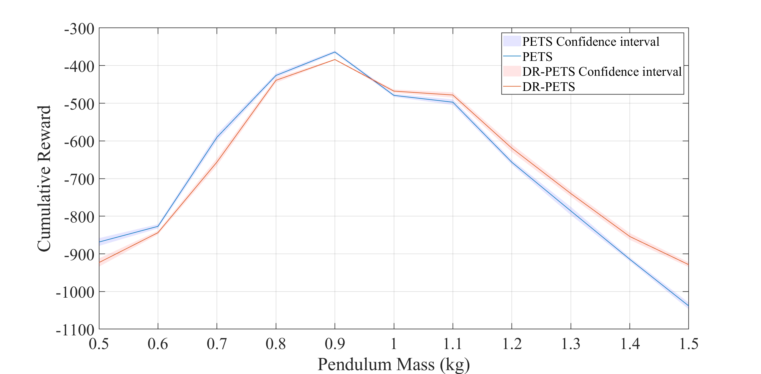
Figure 1: Total episodic reward obtained by the PETS (in blue) and DR-PETS (in red) for perturbation of pendulum mass. Shaded region denotes half of one standard error.

The plot in figure 1 is obtained after 50 simulations for each mass perturbation. The performance difference between PETS and DR-PETS is under parameter perturbations is marginal, although the proposed algorithm exhibits more robustness to model parameter uncertainty. Indeed, when the mass value is higher than 1 kg, the DR-PETS reaches slight higher cumulative reward.

IV-B Example: Cartpole task

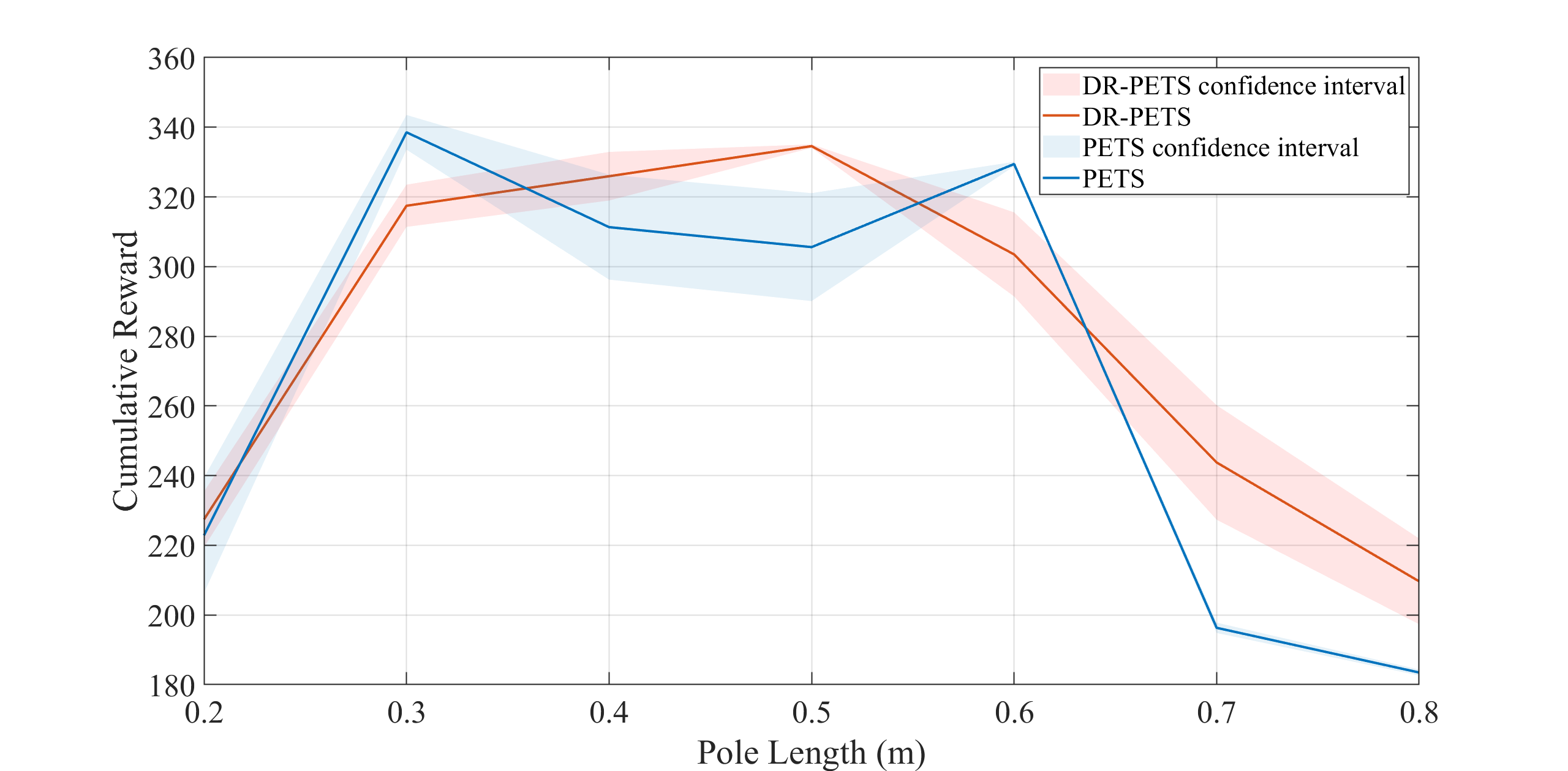
Figure 2: Total episodic reward obtained by the PETS (in blue) and DR-PETS (in red) for perturbation of pole length. Shaded region denotes half of one standard error.

We take a nominal cartpole system with the pole length ($l$) and mass ($m$) being 0.5 m and 1 kg respectively; we employ the algorithm and code provided by [5] to train an ensemble of 5 NNs that estimate the system dynamics. To assess the performance of DR-PETS relative to PETS, we conduct simulations involving cartpole with varying pole lengths, ranging from 0.2 m to 0.8 m, and then assess the total rewards achieved for each length value.

Figure 2 presents cumulative reward comparisons of DR-PETS and PETS over 50 simulations against length perturbation. Beyond a 0.6 m pole, both algorithms show a sharp performance decline, but DR-PETS degrades more gradually, maintaining higher cumulative rewards. Additionally, PETS exhibits a wider confidence interval, suggesting greater performance variability.

References

• [1] E. Garrabe and G. Russo, “Probabilistic design of optimal sequential decision-making algorithms in learning and control,” Annual Reviews in Control, vol. 54, pp. 81–102, 2022.
• [2] P. Yu and H. Xu, “Distributionally robust counterpart in Markov decision processes,” IEEE Transactions on Automatic Control, vol. 61, 01 2015.
• [3] F. D. Lellis, M. Coraggio, G. Russo, M. Musolesi, and M. di Bernardo, “Control-tutored reinforcement learning: Towards the integration of data-driven and model-based control,” in Proceedings of The 4th Annual Learning for Dynamics and Control Conference (R. Firoozi, N. Mehr, E. Yel, R. Antonova, J. Bohg, M. Schwager, and M. Kochenderfer, eds.), vol. 168 of Proceedings of Machine Learning Research, pp. 1048–1059, PMLR, 23–24 Jun 2022.
• [4] P. Klink, Model-Based Reinforcement Learning from PILCO to PETS, p. 165–175. Springer International Publishing, 2021.
• [5] K. Chua, R. Calandra, R. McAllister, and S. Levine, “Deep reinforcement learning in a handful of trials using probabilistic dynamics models,” in Proceedings of the 32nd International Conference on Neural Information Processing Systems, NIPS’18, (Red Hook, NY, USA), p. 4759–4770, Curran Associates Inc., 2018.
• [6] M. Okada and T. Taniguchi, “Variational inference mpc for bayesian model-based reinforcement learning,” in Proceedings of the Conference on Robot Learning (L. P. Kaelbling, D. Kragic, and K. Sugiura, eds.), vol. 100 of Proceedings of Machine Learning Research, pp. 258–272, PMLR, 30 Oct–01 Nov 2020.
• [7] G. Iyengar, “Robust dynamic programming,” Math. Oper. Res., vol. 30, pp. 257–280, 05 2005.
• [8] E. Derman, Y. Men, M. Geist, and S. Mannor, “Robustness and regularization in reinforcement learning,” in NeurIPS 2023 Workshop on Generalization in Planning, 2023.
• [9] R. Gao, “Finite-sample guarantees for wasserstein distributionally robust optimization: Breaking the curse of dimensionality,” Operations Research, vol. 71, no. 6, pp. 2291–2306, 2023.
• [10] E. Derman and S. Mannor, “Distributional robustness and regularization in reinforcement learning,” arXiv preprint arXiv:2003.02894, 2020.
• [11] Z. Liu, Q. Bai, J. Blanchet, P. Dong, W. Xu, Z. Zhou, and Z. Zhou, “Distributionally robust Q-learning,” in International Conference on Machine Learning, pp. 13623–13643, PMLR, 2022.
• [12] F. Zhao and K. You, “Minimax Q-learning control for linear systems using the wasserstein metric,” Automatica, vol. 149, p. 110850, 2023.
• [13] J. Queeney, E. C. Ozcan, I. Paschalidis, and C. Cassandras, “Optimal transport perturbations for safe reinforcement learning with robustness guarantees,” Transactions on Machine Learning Research, 2024.
• [14] C. Mark and S. Liu, “Stochastic MPC with distributionally robust chance constraints,” IFAC-PapersOnLine, vol. 53, no. 2, pp. 7136–7141, 2020.
• [15] P. Coppens and P. Patrinos, “Data-driven distributionally robust MPC for constrained stochastic systems,” IEEE Control Systems Letters, vol. 6, pp. 1274–1279, 2021.
• [16] F. Wu, M. E. Villanueva, and B. Houska, “Ambiguity tube MPC,” Automatica, vol. 146, p. 110648, 12 2022.
• [17] J. Blanchet and K. Murthy, “Quantifying distributional model risk via optimal transport,” Mathematics of Operations Research, vol. 44, no. 2, pp. 565–600, 2019.
• [18] L. Shi and Y. Chi, “Distributionally robust model-based offline reinforcement learning with near-optimal sample complexity,” Journal of Machine Learning Research, vol. 25, no. 200, pp. 1–91, 2024.
• [19] I. J. Goodfellow, J. Shlens, and C. Szegedy, “Explaining and harnessing adversarial examples,” in 3rd International Conference on Learning Representations, ICLR 2015, San Diego, CA (USA), Conference Track Proceedings, 5 2015.
• [20] Z. I. Botev, D. P. Kroese, R. Y. Rubinstein, and P. L’Ecuyer, “The cross-entropy method for optimization,” in Handbook of statistics, vol. 31, pp. 35–59, Elsevier, 2013.