The role of fluctuations in the nucleation process

Abstract

The emergence upon cooling of an ordered solid phase from a liquid is a remarkable example of self-assembly, which has also major practical relevance. Here, we use a recently developed committor-based enhanced sampling method [Kang et al., Nat. Comput. Sci. 4, 451-460 (2024); Trizio et al., arXiv:2410.17029 (2024)] to explore the crystallization transition in a Lennard-Jones fluid, using Kolmogorov’s variational principle. In particular, we take advantage of the properties of our sampling method to harness a large number of configurations from the transition state ensemble. From this wealth of data, we achieve precise localization of the transition state region, revealing a nucleation pathway that deviates from idealized spherical growth assumptions. Furthermore, we take advantage of the probabilistic nature of the committor to detect and analyze the fluctuations that lead to nucleation. Our study nuances classical nucleation theory by showing that the growing nucleus has a complex structure, consisting of a solid core surrounded by a disordered interface. We also compute from the Kolmogorov’s principle a nucleation rate that is consistent with the experimental results at variance with previous computational estimates.

Nucleation is a fundamental physical process which underpins a wide range of phenomena, from the formation of crystals in industrial applications to natural events such as ice formation. Kelton (1991); Oxtoby (1992) Our understanding of the phenomenon is still largely based on classical nucleation theory, which describes the process as due to fluctuations in the under cooled liquid phase in which nuclei of the ordered phase are fleetingly formed. For such fluctuations to eventually lead to crystallization, the size of the nucleus must be such that the free energy gain of the atoms in the crystallite balances the free energy cost of forming an interface between crystallite and liquid. The set of configurations for which this balance occurs identifies the transition state ensemble (TSE).

While in general terms this picture is accepted, the details of how this transition takes place are not fully understood and the fluctuations that drive this phenomenon have not yet been described. Unfortunately, the process of nucleation is difficult to investigate experimentally since it involves studying nanometer scale phenomena that take place in a very short time at random intervals. Molecular dynamics (MD) simulations are in principle well positioned to probe the early stages of nucleation. Mandell, McTague, and Rahman (1977); Stillinger and Weber (1978); Hsu and Rahman (1979) However, nucleation is a rare event that takes place on time scales that cannot be reached by brute-force MD simulations. Giberti, Salvalaglio, and Parrinello (2015); Sosso et al. (2016); Finney and Salvalaglio (2024) This obstacle has not stopped researchers, and a variety of enhanced sampling methods have helped alleviating this problem. Torrie and Valleau (1977); Laio and Parrinello (2002); Invernizzi and Parrinello (2020, 2022); Dellago et al. (1998); Van Erp, Moroni, and Bolhuis (2003); Allen, Valeriani, and Rein Ten Wolde (2009); Espinosa et al. (2016) Thanks to these simulations, much is known about this transition especially when it comes to its prototypical model system i.e. the nucleation of a Lennard-Jones (LJ) liquid. Rein Ten Wolde, Ruiz-Montero, and Frenkel (1996); Moroni, Ten Wolde, and Bolhuis (2005); Trudu, Donadio, and Parrinello (2006); Jungblut and Dellago (2011) Still, as we shall show below, these analyses have been performed on a relatively small set of crystallization trajectories.

Some researchers, have rightly focused their attention on the committor $q(\mathbf{x})$, Kolmogoroff (1931) which is the quantity that most rigorously describes rare events. We recall that given two metastable basins $A$ and $B$, the function $q(\mathbf{x})$ is the probability that a trajectory passing through configuration $\mathbf{x}$ ends in $B$ without having first visited $A$. E and Vanden-Eijnden (2010) Furthermore, computing $q(\mathbf{x})$ allows defining the TSE and it is believed to be the best possible collective variable. Berezhkovskii and Szabo (2005); Ma and Dinner (2005); Li and Ma (2014); He, Chipot, and Roux (2022) Unfortunately, the standard way of computing $q(\mathbf{x})$ involves launching a large number of trajectories, waiting for them to end either in $A$ or $B$ and evaluating from the statistics thus gathered the probability $q(\mathbf{x})$. Moroni, Ten Wolde, and Bolhuis (2005); Trudu, Donadio, and Parrinello (2006); Jungblut and Dellago (2011) In addition to being rather lengthy, this procedure may depend on the limits that are set to the time that one waits before declaring the trajectory committed to either $A$ or $B$. Lazzeri et al. (2023)

This complex procedure is in principle not necessary. In fact, it has been shown that q(x) can be computed using a variational principle due to Kolmogorov. Vanden-Eijnden and Tal (2005); Maragliano and Vanden-Eijnden (2006); Zinovjev and Tuñón (2015); Khoo, Lu, and Ying (2019); Li, Lin, and Ren (2019) Very recently, we have set up an efficient self-consistent procedure that is extremely efficient in computing not only the commitor Kang, Trizio, and Parrinello (2024) but also the free energy, Trizio, Kang, and Parrinello (2024) and like Ref. Vanden-Eijnden and Tal (2005); Maragliano and Vanden-Eijnden (2006); Zinovjev and Tuñón (2015) does not require previous knowledge of the reactive trajectories.

The Kolmogorov’s principle states that $q(\mathbf{x})$ can be computed by minimizing the functional $\mathcal{K}[q(\mathbf{x})]$, Kolmogoroff (1931)

$$\mathcal{K}[q(\mathbf{x})]=\Big{\langle}\big{|}\nabla_{\mathbf{u}}q(\mathbf{x})\big{|}^{2}\Big{\rangle}_{U(\mathbf{x})}$$ (1)

where the average is over the Boltzmann distribution associated with the interatomic potential $U(\mathbf{x})$ at the inverse temperature $\beta$, $\nabla_{\mathbf{u}}$ denotes the gradient with respect to the mass-weighted coordinates, and the boundary conditions $q({\mathbf{x}}_{A})=0$ and $q({\mathbf{x}}_{B})=1$ for configurations $\mathbf{x}_{A}$ and $\mathbf{x}_{B}$ in the two basins are imposed. At the minimum $\mathcal{K}[q(\mathbf{x})]$ is proportional to the reaction rate $\nu$: E and Vanden-Eijnden (2010)

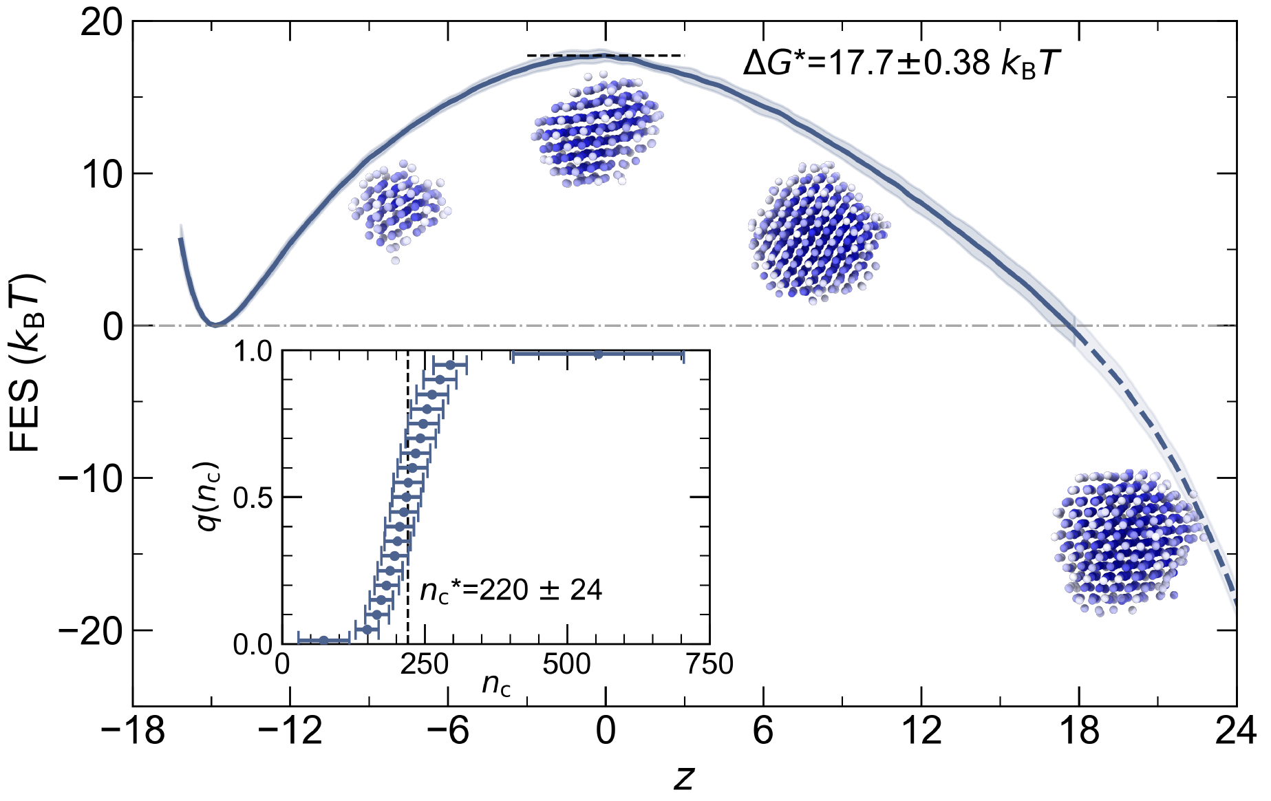
Figure 1: Free energy as function of $z$ for a 2916-atom Lennard-Jones (LJ) system at 0.725 $T_{m}$. The standard deviation over four different OPES+$V_{\mathcal{K}}$ simulations is also shown as a shaded region. We signal with a dashed line the region for $z>18$ where the results might have been influenced by the use of the radius restraint. Snapshots of representative during the nucleation process for different values of $z$, the largest one is taken from the $B$ state. The inset shows the variation of the committor function $q(n_{c})$ projected on the number of atoms in the largest crystalline cluster, $n_{\text{c}}$, as defined in Ref. Rein Ten Wolde, Ruiz-Montero, and Frenkel (1996).

$$\nu=\frac{\mathop{\mathcal{K}[q(\mathbf{x})]}}{\beta\gamma}$$ (2)

In a rare event scenario $q(\mathbf{x})\approx 0$ for $\mathbf{x}\in A$ and $q(\mathbf{x})\approx 1$ for $\mathbf{x}\in B$ thus $\big{|}\nabla_{\mathbf{u}}q(\mathbf{x})\big{|}^{2}$ is strongly peaked at the TSE, the very region that is difficult to sample. In Ref. Kang, Trizio, and Parrinello (2024) this problem was solved by introducing a bias potential dependent on $q(\mathbf{x})$ that is instead able to focus sampling on the transition state (TS) region:

$$V_{\mathcal{K}}(\mathbf{x})=-\frac{1}{\beta}\log(|\nabla q(\mathbf{x})|^{2})$$ (3)

However, since this bias depends on the solution of the variational principle, this appears to be just an academic observation. Luckily, this chicken and egg problem can be solved using an iterative procedure. As shown in Ref. Trizio, Kang, and Parrinello (2024) an extension of the method in combination with On-the-fly Probability Enhanced Sampling (OPES) Invernizzi and Parrinello (2020, 2022) allows a thorough and balanced sampling of both metastable and transition states.

In Ref. Kang, Trizio, and Parrinello (2024); Trizio, Kang, and Parrinello (2024), we have also extended the usual notion of TSE which is defined as the probability distribution:

$$p_{\mathcal{K}}(\mathbf{x})=\frac{|\nabla_{\mathbf{u}}q(\mathbf{x})|^{2}e^{-\beta U(\mathbf{(}x)}}{Z_{\mathcal{K}}}$$ (4)

where $Z_{\mathcal{K}}={\int e^{-\beta U_{\mathcal{K}}(\mathbf{x})}\,\mathrm{d}\mathbf{x}}$ is a normalizing constant. The rational for this choice is that $p_{\mathcal{K}}(\mathbf{x})$ is proportional to the contribution that the trajectories passing via $\mathbf{x}$ gives to the transition rate. This leads to a more nuanced description of the TSE than the standard $q(\mathbf{x})\simeq 0.5$ one.

Since $q(\mathbf{x})$ changes rapidly, we often plot the result as a function of the following logarithmic transformation of the committor $z(\mathbf{x})=\log{\big{(}\frac{q(\mathbf{x})}{1-q(\mathbf{x}\big{)}}\big{)}}$. This transformation has two positive effects, it helps handling the numericsKhoo, Lu, and Ying (2019); Trizio, Kang, and Parrinello (2024) and allows resolving better the TS region. Another helpful numerical trick is to minimize the functional $\log\mathcal{K}[q(\mathbf{x})]$ rather than the original one (see SI Sec. S3). The two functionals share the same minimum since $\mathcal{K}[q(\mathbf{x})]$ is positive definite and the logarithm is a monotonously growing function of its argument.

In this paper we demonstrate that our new method Kang, Trizio, and Parrinello (2024); Trizio, Kang, and Parrinello (2024) is able to tackle efficiently a real-life nucleation problem. In particular, we study here a Lennard-Jones system whose $\epsilon$ and $\sigma$ values have been fixed to values appropriate to argon. In addition we show that this method offers a tool to analyze the liquid fluctuations along the nucleation process and to derive a precise definition of the growing nucleus. Finally we show how from the Kolmogorov’s approach one can determine the nucleation rate of the system.

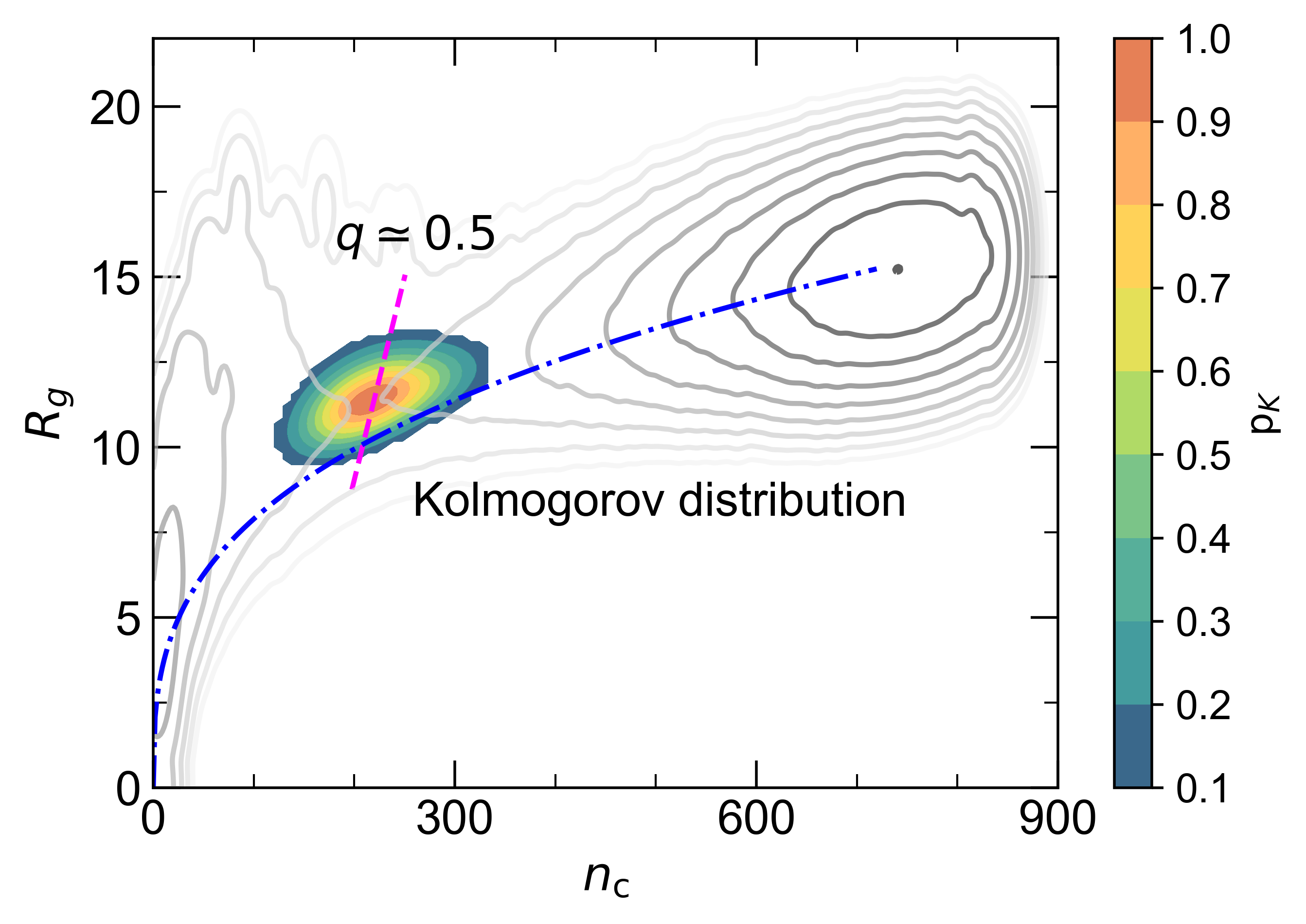
Figure 2: Distribution density of TSE (see Eq. 4) projected in the $n_{\text{c}}$, $R_{g}$ plane. The gray lines are free energy levels, the magenta dashed line shows the isocommittor line $q({n_{c},R_{g}})=0.5$. The blue dashed-dotted line shows the size-scaling $R_{g}\propto n_{\text{c}}^{1/3}$ where the proportionality constant is fitted to state $B$.

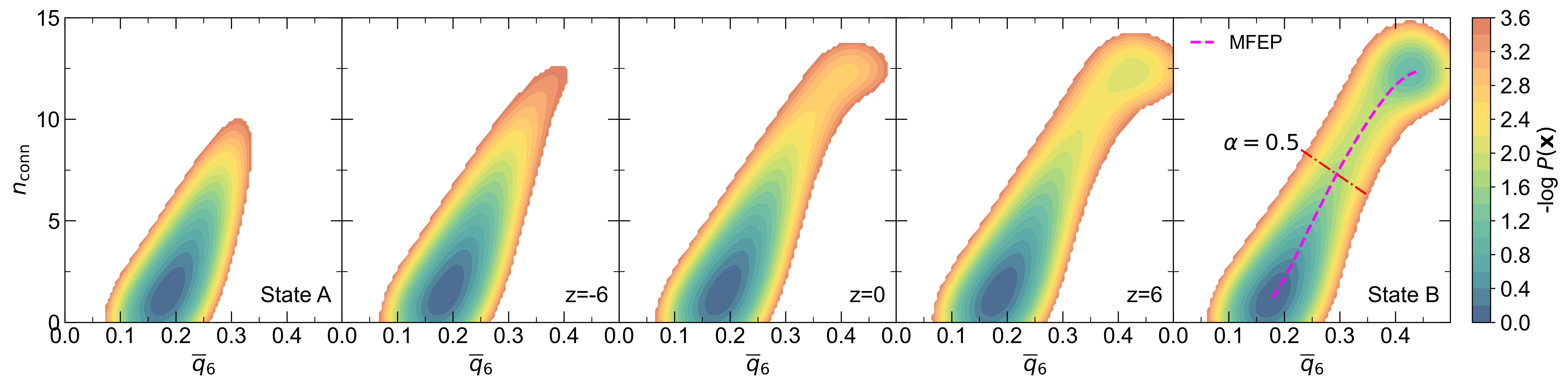
Figure 3: Joint probability distribution of $\overline{q}_{6}$ and $n_{\text{conn}}$ at different values of $z$. The magenta dashed line shows the highest probability path of the multi-modal distribution. For state $B$ the $\alpha=0.5$ is indicated with a magenta dotted line.

When studying crystallization, it is usually assumed that the initial state $A$ is the liquid and the final state $B$ the fully crystallized simulation box. Piaggi, Valsson, and Parrinello (2017); Niu, Yang, and Parrinello (2019); Deng, Du, and Li (2021) Since our focus is on studying the TSE and the reactive process, we depart from this procedure and follow the crystallization process until a sufficiently large crystallite is nucleated. The size of this end crystallite is chosen such that it will irreversibly evolve towards the ordered state. This approach reduces free energy difference $\Delta G_{A-B}$ and accelerates convergence. In such a way, we also reduce the finite size effects that might arise from the size of the growing nucleus and its associated perturbation to the liquid structure being larger than the simulation box, and by the imposition periodic boundary conditions. The latter implies that the final crystalline configuration has to be commensurate with the simulation box. If the crystallization axis are not aligned properly and the number of atoms is not correctly chosen, this can lead to defective structures. The formation of such defective structures can be prevented by the use of custom designed collective variables, however, this might induce some elements of artificiality. Karmakar et al. (2021); Deng et al. (2023) In the SI Sec. S1 we illustrate how the $B$ state is generated.

In order to solve the Kolmogorov variational problem, we express $q(\mathbf{x})$ as a feed forward Neural Network whose features are taken from the vast literature on the problem. Jung et al. (2023) In particular, we use as descriptors the Steinhardt parameter ${q}_{6}^{i}$, Steinhardt, Nelson, and Ronchetti (1983) its locally averaged value $\overline{q}_{6}^{i}$, and pair entropy $s_{S}^{i}$ Piaggi, Valsson, and Parrinello (2017); Piaggi and Parrinello (2017) (see SI Sec. S2). The rational behind this choice is that we want to describe the balance between enthalpy and entropy that characterize the transition, and these two sets of descriptors can be thought of as proxies these two quantities. The numerical details of the self-consistent iterative procedure can be also found in the SI Sec. S3.

In Fig. 1 we present the free energy as a function of $z$ and the committor projected along the number of crystal-like atoms in the largest solid cluster $n_{\text{c}}$ as conventionly done Rein Ten Wolde, Ruiz-Montero, and Frenkel (1996) (see SI Sec. S2.3). The marginal of the committor relative to $n_{\text{c}}$, $q(n_{\text{c}})$, exhibits the expected step-like behavior, and the critical nucleus estimated from $q(n_{\text{c}}^{*})=0.5$ is $n_{\text{c}}^{*}$=220 $\pm$ 20, in agreement with $n_{\text{c}}^{*}$ = 240 $\pm$ 34 in Ref. Trudu, Donadio, and Parrinello (2006). From the free energy plot as a function of $z$ the barrier to nucleation can be estimated to be $\Delta G^{*}=17.7\pm 0.38$ $k_{\text{B}}T$, where $T=0.725\,T_{m}$ is the simulation temperature and $T_{m}$ is the LJ melting temperature. This value is in good agreement with previous estimate of $\Delta G^{*}$ = 18.4 $\pm$ 2 $k_{\text{B}}T$. Trudu, Donadio, and Parrinello (2006)

Having satisfied ourselves of the validity of our approach we use it to better understand the nucleation process. We start by analyzing the TSE as defined by $p_{\mathcal{K}}(\mathbf{x})$ in Eq. 4, and project our result on the space spanned by the number of crystal-like atoms $n_{\text{c}}$ and the associated gyration ratio $R_{g}$. The TSE thus defined aligns with the minimum free energy path. In contrast if we were to use to define the TSE the standard $q(\mathbf{x})\simeq 0.5$ criterion, we would have found as TSE a line that is almost orthogonal to minimum free energy path. It is also interesting to observe that TSE does not follow the $R_{g}\propto n_{\text{c}}^{1/3}$ line, suggesting the critical nuclei are not spherical. A more detailed analysis of the TSE can be found in the SI Sec. S4 where the gyration ratio definition is reported in the SI Sec. S2.4.

We now proceed to study the fluctuations in local liquid order that accompany nucleation. This is made possible by our probabilistic approach and is facilitated by the fact that the variable $z(\mathbf{x})$ induces a natural ordering along the reactive event. We shall describe the local order by the joint distribution of $\overline{q}_{6}$ Steinhardt, Nelson, and Ronchetti (1983) and $n_{\text{conn}}$ Rein Ten Wolde, Ruiz-Montero, and Frenkel (1996) and follow how this distribution evolve as a function of $z$. Already in the under cooled liquid state regime, this distribution exhibits a tail towards larger values of $\overline{q}_{6}$ and $n_{\text{conn}}$. As nucleation progresses, this tail grows, and approximately at $z=0$, the distribution becomes multimodal, with a second peak corresponding to the emergence of well-defined growing nuclei. To simplify the analysis, we project the two-dimensional distribution along the line $\alpha(\overline{q}_{6},n_{\text{conn}})$ of highest probability, following a standard procedure used for analyzing multidimensional free energy surfaces E, Ren, and Vanden-Eijnden (2002) (see Fig. 3).

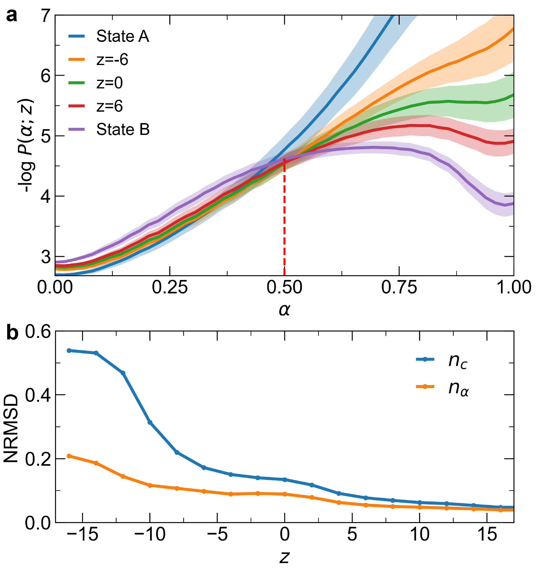
Figure 4: a) Probability distribution $-\text{log}\,P(\alpha;z)$ as function of $\alpha$. b) Normalized root mean square deviation (NRMSD) of $n_{\text{c}}$ and $n_{\alpha}$ along $z$.

As shown in Fig. 4a, the $\alpha$ coordinate reveals a clear bimodal distribution distinguishing two phases. The critical value $\alpha=\frac{1}{2}$ separates the liquid-like regime ($\alpha<\frac{1}{2}$) from the solid-like regime ($\alpha>\frac{1}{2}$). Thus, we use the $\alpha>\frac{1}{2}$ criteria to identify the configurations that belong to the growing crystalline nucleus. The bimodal character of the local order fluctuation suggests that all the atoms in the side peak $n_{\alpha}$ should be counted when measuring the size of the growing nucleus. The usefulness of this choice is evident in the substantially reduced uncertainty in $z(n_{\alpha})$ compared to $z(n_{\text{c}})$ (see SI Sec. S5), as measured by a much reduced normalized root mean square error (see Fig. 4b). Since the fluctuation of $n_{\alpha}$ are clearly smaller than those of $n_{\text{c}}$, it follows that the physics of the transition is better described by $n_{\alpha}$.

Finally, we use Eq.2 to calculate the reaction rate $\nu$ from which the nucleation rate $J$ can be estimated. This formula has been derived under the hypothesis of overdamped dynamics, and give for $\nu$ a result that is proportional to $\frac{1}{\gamma}$. If we want to use Eq.2 to compute $\nu$ we need to estimate what is the effective value of $\gamma$ in our standard Newtonian MD run. This can be done using a procedure that in the past has been applied in dynamical Monte Carlo. Binder (1995) We first measure the diffusion coefficient in the undercooled liquid with our standard unbiased MD algorithm, then we perform a number of overdamped Langevin dynamics simulations for different values of $\gamma$, choosing for $\gamma$ the value that best reproduces the computed diffusion coefficient. In such a fashion, we get for $J$ the value $\approx 1.9\times 10^{30}\,\text{m}^{-3}\text{s}^{-1}$ in a much better agreement with the experimental data ($1.5\text{ - }6.2\times 10^{30}\,\text{m}^{-3}\text{s}^{-1}$) Möller et al. (2024) than previous theoretical estimation of $3.1\times 10^{32}\,\text{m}^{-3}\text{s}^{-1}$. Tipeev, Zanotto, and Rino (2018) Details of the estimation of nucleation rate can be found in SI Sec.S6.

In this work, we found that the method is highly effective in describing nucleation and above all capable of describing in detail the fluctuations that eventually lead to the phase transition. The success of our approach opens the way to many developments that will be explored in the future. We only quote here the possibility applying a transfer learning approach similar to that of Ref. Das et al. (2024) to study with little effort system behavior across different temperatures and across families of similar compounds.

Code and Data Availability

The NN-based committor models are based on the Python machine learning library PyTorch. Paszke et al. (2019) The specific code for the definition and the training of the model is developed in the framework of the opensource mlcolvar Bonati et al. (2023) library. The committor-based enhanced sampling simulations have been performed using LAMMPS Thompson et al. (2022) patched with PLUMED Tribello et al. (2014) 2.9. All the reported molecular snapshots have been produced using the ovito. Stukowski (2010)

Bibliography

Supporting Information

S1 Generating the $B$ state

We implemented a radius restraint as shown in Fig. S1, to accelerate the convergence of OPES simulations and prevent the system from fully crystallizing. First, atoms in the system were identified as solid-like as defined in Eq. S7. It should be noted that this $n_{\overline{q}_{6}}$ differs from the $n_{c}$ and our probability-based $n_{\alpha}$, serving merely as a simplified method to distinguish solid-like atoms. An arbitrarily chosen atom was then designated as the reference center of the nucleus, with atoms within a radius $R_{\text{wall}}$ from this reference atom defined as the inner part, and those beyond it constituting the outer part. A bias potential, $V_{\text{wall}}$, was subsequently applied to the atoms in the outer part to suppress cluster growth beyond the radius $R_{\text{wall}}$. The bias potential is expressed as:

$$V_{\text{wall}}=\begin{cases}k(n_{\overline{q}_{6}}^{\text{out}}-n_{\text{th}})^{2},&\text{if }n_{\overline{q}_{6}}^{\text{out}}>n_{\text{th}},\\ 0,&\text{if }n_{\overline{q}_{6}}^{\text{out}}\leq n_{\text{th}}.\end{cases}$$ (S1)

where $k=0.02\,\text{kJ/mol}$, and a threshold value of $n_{\text{th}}=200$ was selected to ensure that the bias is activated only when the radius of cluster exceeds $R_{\text{wall}}$. Furthermore, state $B$ is defined as a sufficiently large crystallite that stabilizes under the influence of $V_{\text{wall}}$, meaning it will irreversibly transition to the ordered state when simulated with conventional MD.

To evaluate the effect of the radius restraint, we performed a series of simulations incorporating OPES with an optimal Kolmogorov bias $V_{\mathcal{K}}$, and additionally $V_{\text{wall}}$ with $R_{\text{wall}}$ values ranging from 16.5 Å to 18 Å. The time evolution of the CV $z$ under different $R_{\text{wall}}$ conditions is presented in Fig. S2, while the corresponding FES are shown in Fig. S3. As shown in Fig. S3, the FES exhibits gradual convergence with increasing $R_{\text{wall}}$. With a radius restraint of $R_{\text{wall}}=18\,\text{\r{A}}$, the FES in the region where $z<18$ closely matches that obtained at $R_{\text{wall}}=17.5\,\text{\r{A}}$. As a result, we adopted $R_{\text{wall}}=18\,\text{\r{A}}$ for all subsequent analyses, ensuring that the inner part encompasses the size of the critical nuclei while minimizing boundary effects. All the statistical analyses were conducted within the region $z<18$ which remains unaffected by the bias of radius restraint. To further ensure accuracy, configurations with $V_{\text{wall}}>0$ were excluded from the statistical calculations.

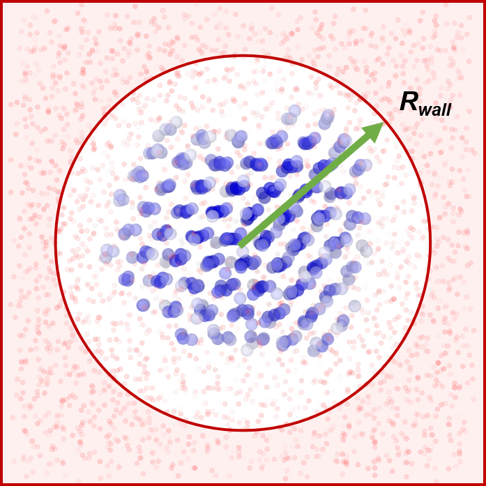
Figure S1: Diagram of the radius restraint setup. Only the atoms in the outer region (shown in red with transparency) contribute to $n_{\overline{q}_{6}}^{\text{out}}$, where the bias potential $V_{\text{wall}}$ is applied. This restraint prevents the inner region from driving complete crystallization of the system.

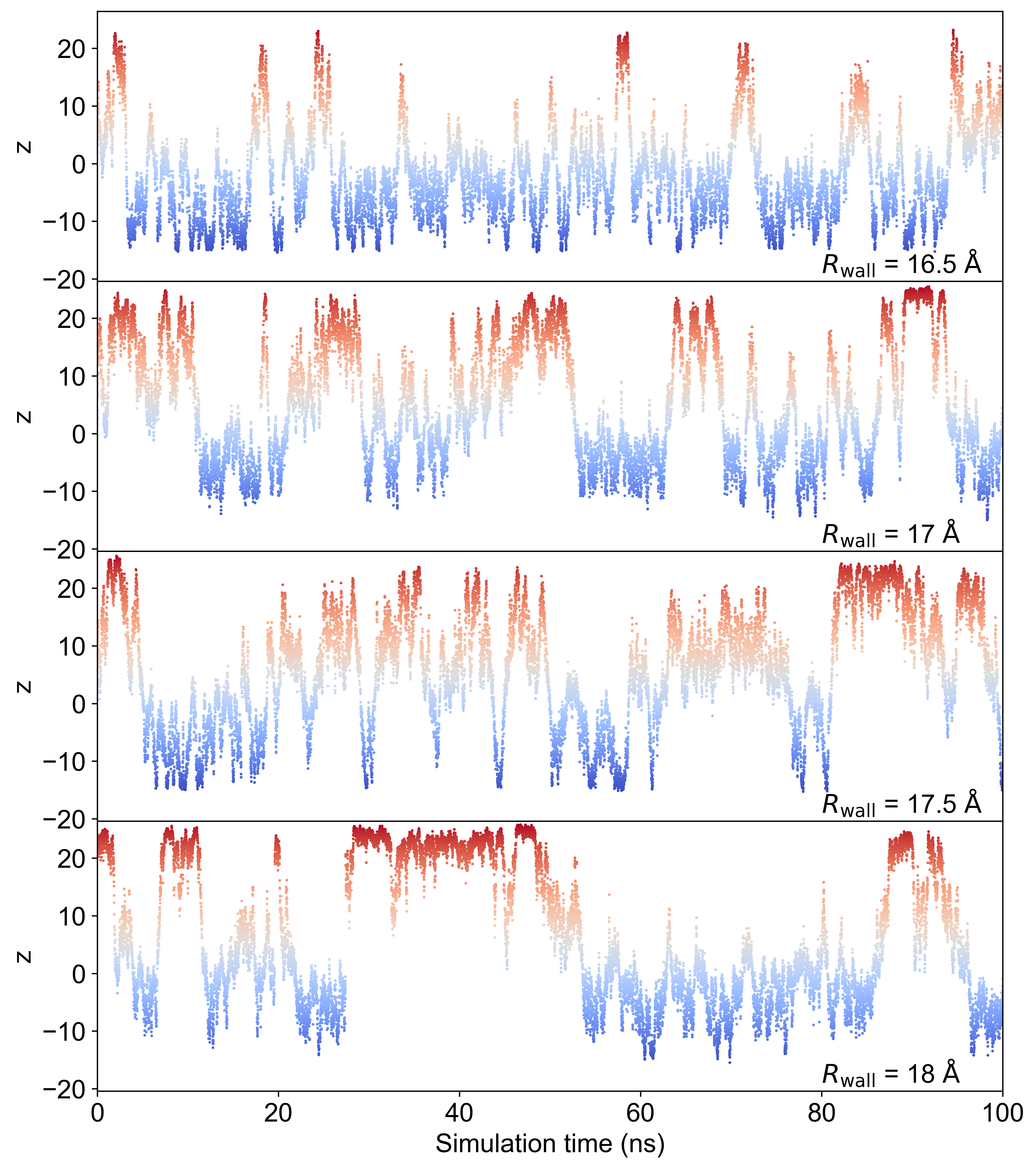
Figure S2: Evolution of $z$ CV as function of time for the 2916-atom LJ system at 67 K with the radius restraint of $R_{\text{wall}}$ = 16.5 Å, 17 Å, 17.5 Å, and 18 Å.

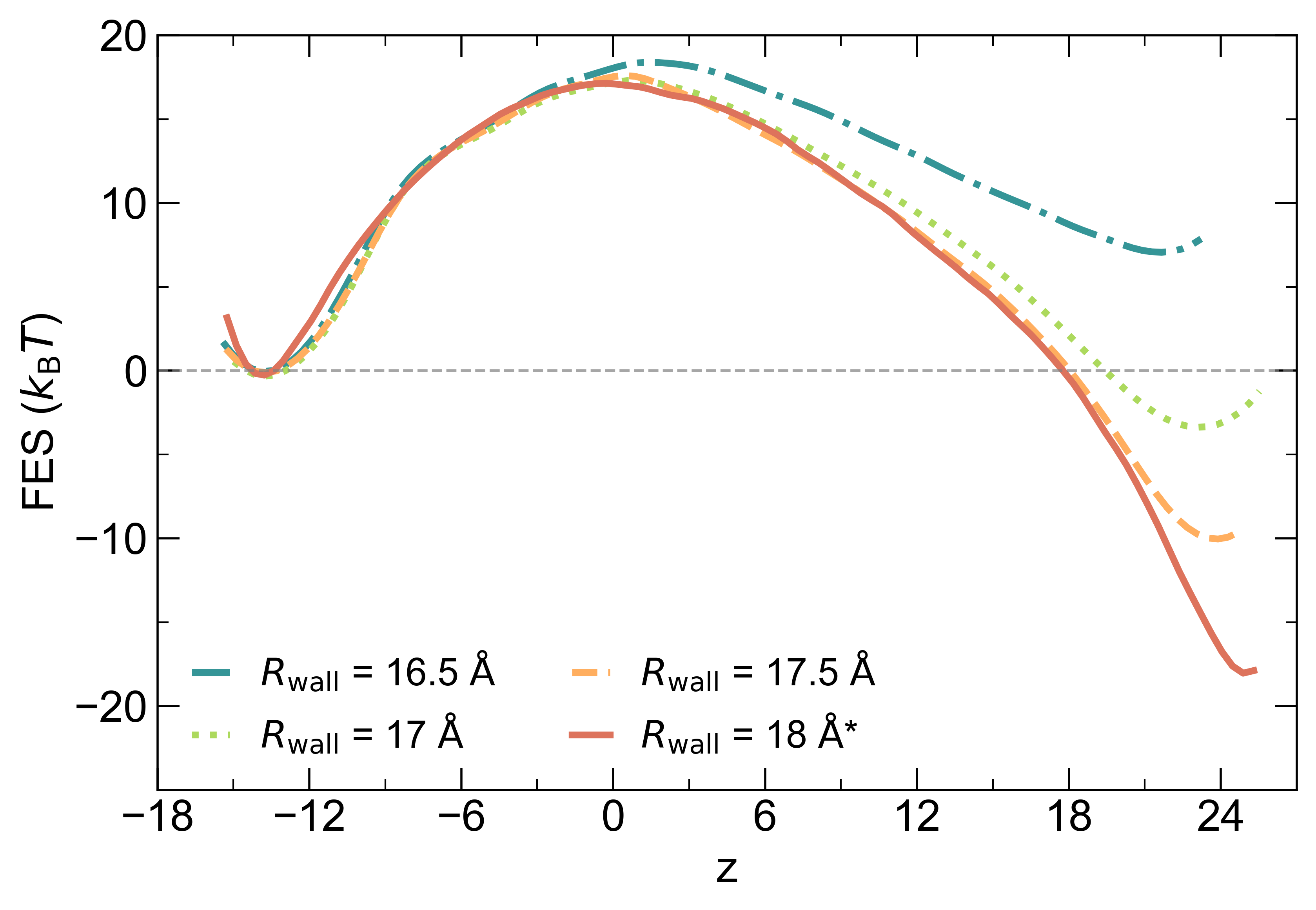
Figure S3: Free energy surface of the 2916-atom LJ system at 67 K with the radius restraint of $R_{\text{wall}}$ = 16.5 Å, 17 Å, 17.5 Å, and 18 Å.

S2 Symbols and their definition

S2.1 Steinhardt bond order descriptors

We selected a set of Steinhardt bond order descriptors Steinhardt, Nelson, and Ronchetti (1983); Rein Ten Wolde, Ruiz-Montero, and Frenkel (1996); Lechner and Dellago (2008) to characterize atomic local environment for LJ system. First, the complex vector of each atom, $q_{lm}(i)$, is defined as:

$$q_{lm}(i)=\frac{\sum_{j}\sigma(r_{ij})Y_{lm}(\mathbf{(}r_{ij}))}{\sum_{j}\sigma(r_{ij})}.$$ (S2)

where $Y_{lm}$ are spherical harmonics with degree of $l$, vector $\mathbf{(}r_{ij})$ connects atom $i$ and $j$, and $N_{b}$ is the number of neighbors of atom $i$. A switching function is used to make the function decays smoothly to 0 at the cutoff of first coordinate shell,

$$\sigma(r_{ij})=\begin{cases}\frac{1-(r_{ij}/r_{c})^{6}}{1-(r_{ij}/r_{c})^{12}},&\text{if }r_{ij}<r_{\text{max}},\\ 0,&\text{if }r_{ij}\geq r_{\text{max}}.\end{cases}$$ (S3)

where $r_{c}=4.5$ Å is set to ensure the contribution reduced smoothly at $r_{\text{max}}=5.1$ Å, corresponding to the first minimum of the radial distribution function of the liquid. Then, the $l$ order Steinhardt parameter $q_{l}(i)$ is given as:

$$q_{l}(i)=\sqrt{\frac{4\pi}{2l+1}\sum_{m=-l}^{l}|q_{lm}(i)|^{2}}.$$ (S4)

To improve its performance, we can replace the $q_{lm}$ vectors of atom $i$ by the average over its nearest neighbors and itself with the same switching function as Eq. S3,

$$\overline{q}_{lm}(i)=\frac{\sum_{j}\sigma(r_{ij})\sum_{m=-6}^{6}q_{6m}^{*}(i)q_{6m}(j)}{\sum_{j}\sigma(r_{ij})}.$$ (S5)

Then, the local averaged Steinhardt parameter, $\overline{q}_{l}(i)$, can be given as:

$$\overline{q}_{l}(i)=\sqrt{\frac{4\pi}{2l+1}\sum_{m=-l}^{l}|\bar{q}_{lm}(i)|^{2}},$$ (S6)

While $q_{l}(i)$ holds the structure information of the first coordinate shell around atom $i$, its averaged form $\overline{q}_{l}(i)$ incorporates the second shell, offering a more comprehensive description of the local environment. The histogram of $q_{6}^{i}$ and $\overline{q}_{6}^{i}$ are estimated using a Gaussian expansion to ensure continuous derivatives and are presented in Fig. S4a and b, respectively.

Given the critical role of the number of solid-like atoms in classical nucleation theory, we define $n_{\overline{q}_{6}}$ as a smooth descriptor approximating the count of atoms with $\overline{q}_{6}^{i}>0.325$, achieved by combining it with a switching function. This provides a simplified yet effective measure of the number of solid-like atoms, expressed as:

$$n_{\overline{q}_{6}}=\sum_{i}\frac{1-(\overline{q}_{6}^{i}/0.325)^{6}}{1-(\overline{q}_{6}^{i}/0.325)^{12}}$$ (S7)

For the Steinhardt bond-order parameters, we utilize a total of five bins from the histograms of $q_{6}^{i}$ and $\overline{q}_{6}^{i}$, along with the averaged $\overline{q}_{6}$ and $n_{\overline{q}_{6}}^{\text{in}}$ as descriptors.

S2.2 Pair Entropy

To better capture longer range atomic environment, we take the entropy-based fingerprint Piaggi and Parrinello (2017) to further identify local structures and used as descriptors for the training of committor model. The projection of an approximate evaluation of the entropy on atom $i$ can be expressed as:

$$s_{S}^{i}=-2\pi\rho k_{B}\int_{0}^{r_{m}}[g_{m}^{i}(r)\ln g_{m}^{i}(r)-g_{m}^{i}(r)+1]r^{2}dr,$$ (S8)

where $r_{m}$ = 7.5 Å is an upper integration limit , and $g_{m}^{i}(r)$ is the radial distribution function centered at the atom $i$ given as:

$$g_{m}^{i}(r)=\frac{1}{4\pi\rho r^{2}}\sum_{j}\frac{1}{\sqrt{2\pi\sigma^{2}}}e^{-(r-r_{ij})^{2}/(2\sigma^{2})},$$ (S9)

where $j$ are the neighbors of atom $i$, $r_{ij}$ is the distance between atoms $i$ and $j$, and $\sigma$ = 0.5 Å is a broadening parameter. The histogram of $s_{S}^{i}$ is estimated using a Gaussian expansion and is shown in Fig. S4c. The values of five bins from the histograms $s_{S}^{i}$ are selected as descriptors.

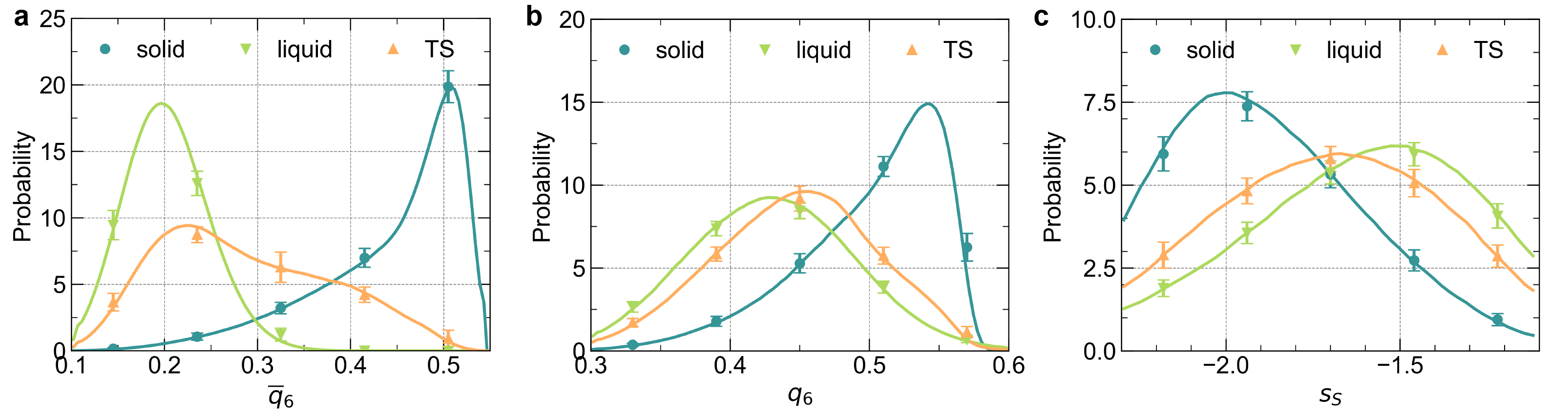
Figure S4: Histogram of a) $\overline{q}_{6}^{i}$,b) ${q}_{6}^{i}$, and c) $s_{S}^{i}$. Dotted point refer to the average of 5 bins selected as the descriptors.

S2.3 Counting the number of crystal-like atoms in the growing nuclei; $n_{\text{c}}$

We first identified crystal-like atoms within the largest cluster, $n_{\text{c}}$, based on the criterion introduced in Ref. Rein Ten Wolde, Ruiz-Montero, and Frenkel (1996). Two particles are classified as neighbors if their distance is less than 5 Å. The normalized scalar product of the complex vectors $q_{6m}$ for neighboring particles $i$ and $j$ is then given by:

$$S_{ij}=\frac{\sum_{m=-6}^{6}q_{6m}(i)q_{6m}^{*}(j)}{(\sum_{m=-6}^{6}|q_{6m}(i)|^{2})^{1/2}(\sum_{m=-6}^{6}|q_{6m}(j)|^{2})^{1/2}},$$ (S10)

which quantifies the degree of structural correlation between the local environments of particles $i$ and $j$. If this scalar product is larger than 0.5, the two particles are considered to be connected to each other. A particle is identified as crystal-like, if its number of connections $n_{\text{conn}}$ is larger than 8. Crystal-like particles that are neighbors belong to the same cluster. The size of the largest cluster is denoted as $n_{\text{c}}$.

S2.4 Gyration radius and asymmetry ratio; $R_{g}$

To gain deeper insight into the evolution of cluster shapes during the nucleation process, we analyzed the gyration matrix and its associated gyration radius and asymmetry ratio. Jungblut and Dellago (2011) The gyration matrix $\underline{R}_{g}$ of a cluster is computed as:

$$\underline{R}_{g}^{2}=\frac{1}{N}\sum_{i=1}^{N}(\mathbf{r}_{i}-\mathbf{r}_{\text{com}})\otimes(\mathbf{r}_{i}-\mathbf{r}_{\text{com}}),$$ (S11)

where $N$ is the number of atoms forming the cluster, $\mathbf{r}_{i}$ is the position of the particles belonging to the cluster, and $\mathbf{r}_{\text{com}}$ is the position of the center of mass of the cluster. The gyration radius $R_{g}$ is then given as:

$$R_{g}=[\langle R_{g,1}^{2}\rangle+\langle R_{g,2}^{2}\rangle+\langle R_{g,3}^{2}\rangle]^{1/2}.$$ (S12)

Furthermore, the shape of the cluster was characterized by the asymmetry ratio $R_{g,3}/R_{g,1}$:

$$R_{g,3}/R_{g,1}=[\frac{\langle R_{g,3}^{2}\rangle}{\langle R_{g,1}^{2}\rangle}]^{1/2}.$$ (S13)

Detailed results of the evolution of gyration radius and asymmetry ratio are discussed in Sec. S4.

S3 Committor model training

S3.1 Learning the committor function

We follow the similar self-consistent procedure described in Ref. Kang, Trizio, and Parrinello (2024); Trizio, Kang, and Parrinello (2024) for solving the comiitor function. The committor function is represented as a NN $q_{\theta}(\mathbf{x})=q(\mathbf{d}(\mathbf{x}))$ with learnable parameters $\theta$ that takes as inputs a set of physical descriptors $\mathbf{d}(\mathbf{x})$. The optimization of $q_{\theta}^{n}(\mathbf{x})$, at iteration $n$, is based on the minimization of an objective function $\mathcal{L}$ that formalizes the variational principle of Eq. 1, $\mathcal{L}_{v}$, and its boundary conditions $\mathcal{L}_{b}$. The relatively high nucleation barrier at temperature below $T_{m}$ Moroni, Ten Wolde, and Bolhuis (2005); Trudu, Donadio, and Parrinello (2006) may led to significant imbalance between $\mathcal{L}_{v}$ and $\mathcal{L}_{b}$. Specifically, the variational loss was several orders of magnitude smaller than the boundary loss, resulting in suboptimal performance.

To address this issue, here we modified an optimized logarithmic loss function as,

$$\mathcal{L}=\log\mathcal{L}_{v}+\alpha\mathcal{L}_{b}$$ (S14)

which is relatively scaled by the hyperparameter $\alpha$. The $L_{v}$ term derives from the variational principle and reads:

$$\mathcal{L}_{v}=\frac{1}{N_{n}}\sum_{i=1}^{N_{n}}w_{i}|\nabla_{\mathbf{u}}q(\mathbf{x}_{i})|^{2},$$ (S15)

where the weights $w_{i}$ weigh each configuration $\mathbf{x}_{i}$ to natural Boltzmann weight. The $L_{b}$ term enforces the boundary conditions $q(\mathbf{x}_{A})=0$ and $q(\mathbf{x}_{B})=1$ as:

$$\mathcal{L}_{b}=\frac{1}{N_{A}}\sum_{i\in A}(q(\mathbf{x}_{i})-0)^{2}+\frac{1}{N_{B}}\sum_{i\in B}(q(\mathbf{x}_{i})-1)^{2}.$$ (S16)

As discussed in Ref. Trizio, Kang, and Parrinello (2024), the $\mathcal{L}_{b}$ term was evaluated using a labeled dataset of $N_{A}$ and $N_{B}$ configurations collected at the first iteration via unbiased simulations. In contrast, the $\mathcal{L}_{v}$ term at the first iteration was solely influenced by these unbiased labeled configurations, whereas from the second iteration onward, only the biased configurations contributed to the $\mathcal{L}_{v}$ term. This strategy can help get rid of the slowdown arising from the incorrect weights of the unbiased configurations in the dataset.

S3.2 Self-consistent iterative procedure

In Ref. Kang, Trizio, and Parrinello (2024), we demonstrated that the variational principle, combined with the sampling of the Kolmogorov ensemble, can be used in a self-consistent iterative framework to obtain the committor function with the assistance of machine learning. This iterative procedure alternates between training a NN-based variational parametrization of the committor function and generating progressively improved data through sampling under the influence of the TS-oriented Kolmogorov bias $V_{\mathcal{K}}(\mathbf{x})$. In this work, the procedure begins with statistical sampling driven by $V_{\mathcal{K}}^{n}(\mathbf{x})$ to estimate the functional $\mathcal{K}[q(\mathbf{x})]$ and obtain an initial approximation of the committor $q^{0}(\mathbf{x})$. Subsequently, $q(\mathbf{x})$ is refined iteratively using a combination of the Kolmogorov bias $V_{\mathcal{K}}^{n}(\mathbf{x})$ and an adaptive bias $V_{\text{OPES}}(\mathbf{x})$Trizio, Kang, and Parrinello (2024). A schematic overview of the iterative steps is provided as below.

• Step 1: An initial approximation of the committor $q^{0}(\mathbf{x})$ is obtained through an iterative procedure involving the Kolmogorov bias potential $V_{\mathcal{K}}$. At the first iteration ($n=0$), a dataset is generated by performing short unbiased simulations within the metastable basins, and the sampled configurations are labeled accordingly. The initial committor model $q^{0}(\mathbf{x})$ is then trained using configurations $\mathbf{x}^{n}$ and weights $w_{i}^{n}$ obtained under $V_{\mathcal{K}}$, following the variational principle defined in Eq. S14.

• Step 2: Biased simulations are carried out under the combined influence of the Kolmogorov bias potential $V_{\mathcal{K}}^{n}$ and the OPES bias potential $V_{\text{OPES}}^{n}$. The OPES bias acts along the committor-based collective variable $z^{n}(\mathbf{x})$, promoting efficient sampling across the configurational space between metastable states. Meanwhile, the Kolmogorov bias ensures thorough sampling of the TS region, which is essential for refining the committor model via the variational principle.

• Step 3: The sampled configurations are added to the dataset and reweighted using the total effective bias potential $V_{\text{eff}}=V_{\mathcal{K}}+V_{\text{OPES}}$. The reweighting factor is given by $w_{i}^{n}=\frac{e^{\beta V_{\text{eff}}^{n}(\mathbf{x}_{i})}}{\langle e^{\beta V_{\text{eff}}^{n}(\mathbf{x})}\rangle_{U_{\text{eff}}^{n}}}$, where $\beta$ is the inverse temperature. This reweighting step ensures a progressively accurate estimate of the FES as the iterations proceed.

• Step 4: The updated dataset, containing reweighted configurations and their associated weights $w_{i}^{n}$, is used to re-optimize the neural-network-based committor $q^{n}(\mathbf{x})$ using the variational principle of Eq. S14. The refined committor model serves as input for the next iteration from step 2. This iterative process progressively improves the accuracy of both the committor and the estimated FES.

S3.3 Training parameters

To model the committor function $q_{\theta}(\mathbf{x})$ at each iteration, we used $n_{\overline{q}_{6}}^{\text{in}}$, $\overline{q}_{6}$, along with the histograms of $q_{6}^{i}$, $\overline{q}_{6}^{i}$, and $s_{S}^{i}$ as inputs to a NN with the architecture [17, 80, 40, 1], as discussed in Sec. S2. The optimization was performed using the ADAM optimizer with an initial learning rate of $10^{-3}$, modulated by an exponential decay with a multiplicative factor of $\gamma=0.99993$. The training ran for approximately $\sim$50,000 epochs, with the $\alpha$ hyperparameter in the loss function Eq. S14 set to 5. The $K_{m}$ values of the $q_{\theta}(\mathbf{x})$ model trained with different descriptor sets at final iteration are presented in Table S1. The number of iterations, corresponding dataset sizes, $\lambda$ values, and OPES BARRIER parameters used in the biased simulations are summarized in Tables S2 and  S3. Additionally, these tables report the lowest values of the functional $K_{m}$ as a measure of model quality and convergence, along with the simulation time $t_{s}$ and the output sampling time $t_{o}$.

S3.4 OPES+$V_{\mathcal{K}}$ biased simulations

We employed OPES enhanced sampling techniques to investigate the reversible nucleation process of the LJ system. The committor value $z$ was used as the CV to drive the OPES simulations.

In OPES method, the equilibrium probability distribution $P(z)$ is estimated on the fly, and a bias potential $V_{n}(s)$ is constructed to drive $P(z)$ toward a target distribution $P_{\text{tg}}(z)$. Here, we chose the well-tempered distribution Bonomi, Barducci, and Parrinello (2009) as the target:

$$P^{\text{tg}}(s)\propto\left[P(s)\right]^{\frac{1}{\gamma}},$$ (S17)

where $\gamma>1$ is the bias factor. In this framework, the bias potential at the $n$-th iteration is expressed as:

$$V_{n}(s)=\left(1-\frac{1}{\gamma}\right)\frac{1}{\beta}\log\left(\frac{P_{n}(s)}{Z_{n}}+\varepsilon\right),$$ (S18)

where $Z_{n}$ is a normalization factor, $\beta$ is the inverse temperature, and $\varepsilon=e^{-\beta\Delta E/(1-\frac{1}{\gamma})}$ is a regularization parameter that limits the maximum deposited bias $\Delta G$. In this study, we set the kernel deposition frequency to 500 and restricted $\Delta G$ to 15 kJ mol^-1 (corresponding to the STRIDE and BARRIER parameters in the PLUMED input files, respectively).

The sampling density and the time evolution of the $z$ CV are shown in Fig. S5 and Fig. S6, respectively. The convergence of the solid-liquid free energy difference $\Delta G_{A-B}$ is presented in Fig. S7.

For the sampling of dataset, we used LJ parameter for argon, with $\epsilon$ = 119.8 K and $\sigma$ = 3.405 nm. Rowley, Nicholson, and Parsonage (1975) The interaction potential cutoff is set at 9 Å and long-range corrections are considered in the computation of both total energy and pressure. Sun (1998) A timestep of 10 fs was used for the integral of motion in biased simulations. The Nosé-Hoover thermostat Hoover (1985) and Parrinello–Rahman barostat Parrinello and Rahman (1981) were used with a relaxation time of 0.1 ps and 1 ps, respectively. Based on the regression function of melting line in Ref. Mastny and De Pablo (2007), we take T = 67 K referred to 0.725 $T_{m}$ at P = 0.25 kbar for all the simulations in current work.

Table S1: Comparison of the performances of different descriptor sets for LJ system. The descriptor sets discussed in the main text are marked with an asterisk.

Set id	Descriptors $\mathbf{x}$	$K_{m}$
1	$n_{\overline{q}_{6}}^{\text{in}}$, $\overline{q}_{6}$	3.08
2	histogram of $\overline{q}_{6}^{i}$	3.68
3	Set 1 + Set 2	2.82
4	Set 1 + histogram of $q_{6}^{i}$ and $s_{S}^{i}$	2.81
5*	Set 2 + Set 4	2.54

Table S2: Summary of the initial estimation with $V_{\mathcal{K}}$ biased simulations for LJ system.

Iteration	Dataset size	$K_{m}$	$\lambda$	$t_{s}$ [ns]	$t_{o}$ [ps]
0	2000	$9.5\times 10^{11}$	-	2*0.5	0.5
1	6000	$7.3\times 10^{4}$	3	2*0.4	0.2
2	6000	$9.5\times 10^{3}$	2	2*0.4	0.2
3	10000	$6.2\times 10^{3}$	1.2-1.35	4*0.4	0.2

Table S3: Summary of the iterative procedure with OPES+$V_{\mathcal{K}}$ biased simulations for LJ system.

Iteration	Dataset size	$K_{m}$ [au]	OPES BARRIER [kJ/mol]	$t_{s}$ [ns]	$t_{o}$ [ps]
1	22000	835.5	15	4*4	0.4
2	22000	144.7	15	4*10	1
3	22000	3.43	15	2*50	5
4	22000	4.11	15	4*50	10
5	22000	2.54	15	4*100	20

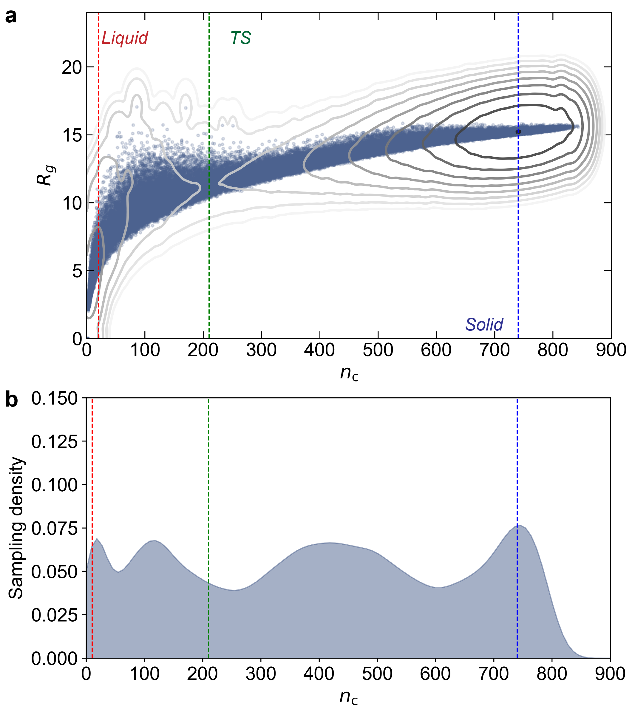
Figure S5: a) Scatter plot of the sampled points under the bias of OPES+$V_{\mathcal{K}}$. In the background, the FES is represented by its isolines. b) Distribution of the sampled configurations along $n_{\text{c}}$ in the simulation. This picture demonstrates that the sampling is uniform in both metastable and TS region.

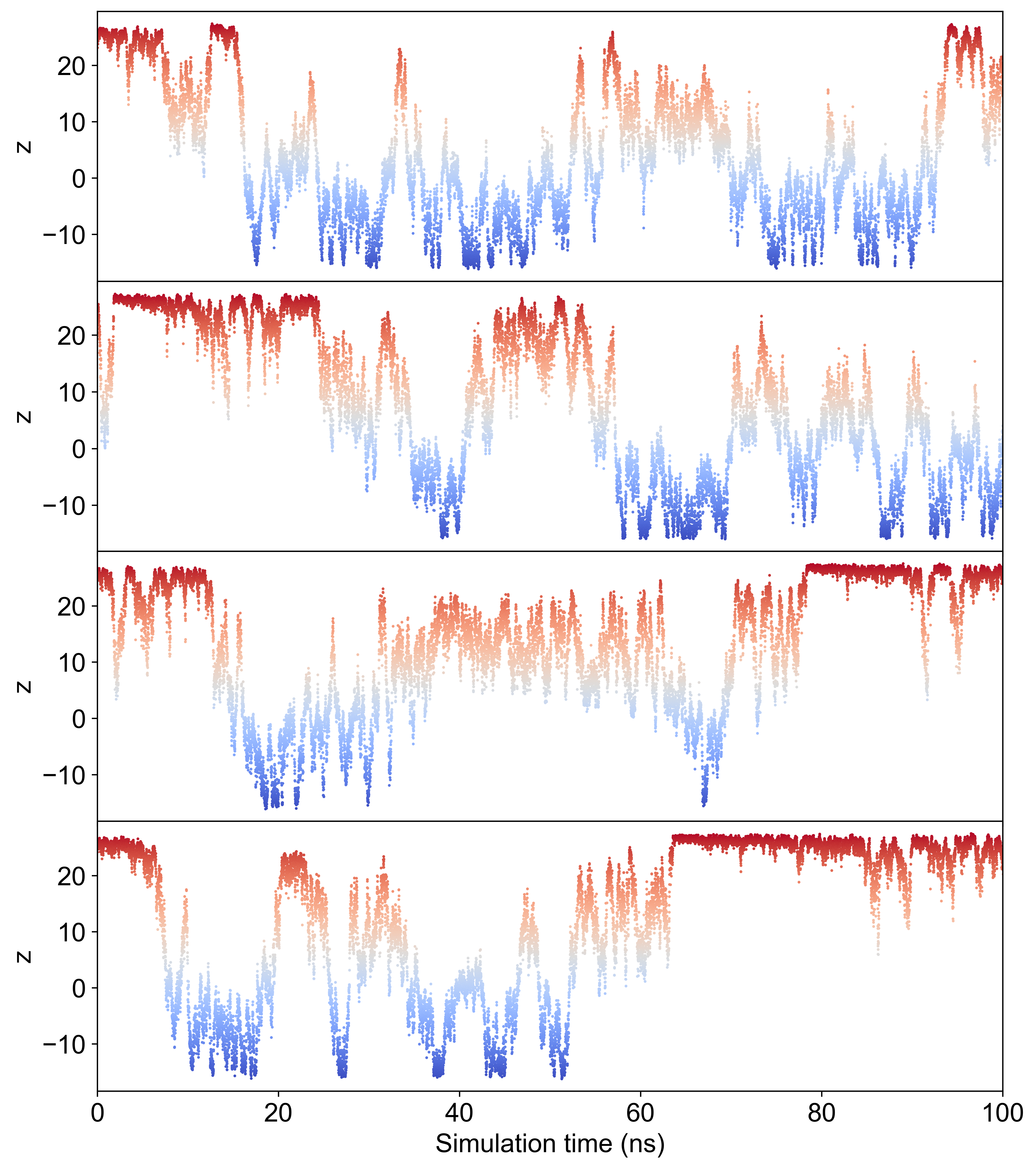
Figure S6: Evolution of $z$ CV as function of time for the 2916-atom LJ system at 67 K. Four independent simulations with different random seeds are shown, demonstrating the efficiency of our sampling method.

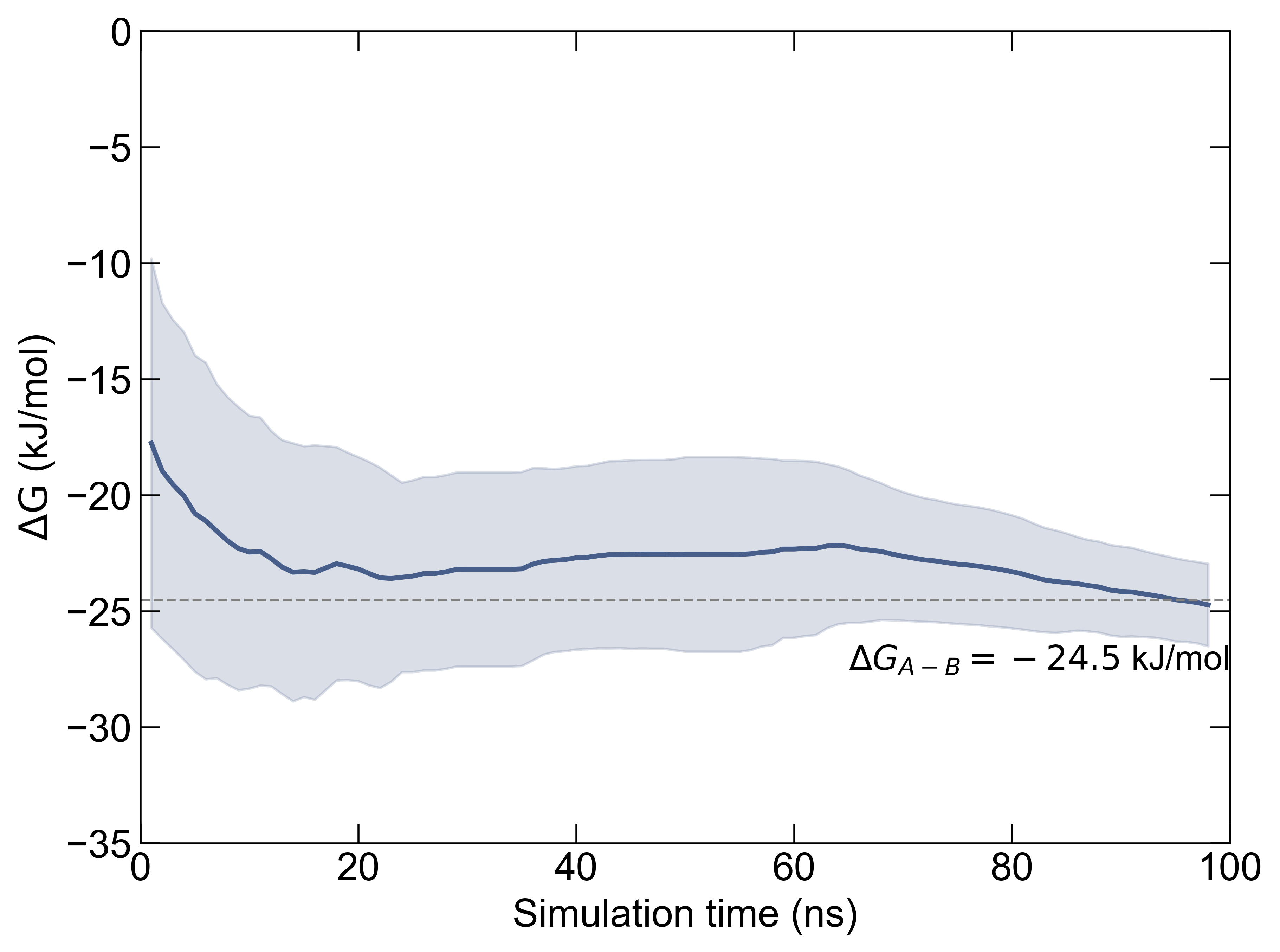
Figure S7: Convergence with simulation time of the estimate $\Delta G_{A-B}$ over four set of OPES+$V_{\mathcal{K}}$ simulations for the 2916-atom LJ system at 67 K.

S4 Analysis of TSE

To investigate the shape evolution and aspherical nature of critical nuclei, we analyzed the TSE defined by $p_{\mathcal{K}}(\mathbf{x})$ in Eq. 4, projecting the results onto spaces spanned by $n_{\text{c}}$, $n_{\alpha}$, and the asymmetry ratio $R_{g,3}/R_{g,1}$. As shown in Fig. S8a and b, the $p_{\mathcal{K}}$-based TSE in both the $n_{\text{c}}$-asymmetry ratio plane and $n_{\alpha}$-asymmetry ratio plane reveals a broad distribution of asymmetry ratios, with a central value of $R_{g,3}/R_{g,1}\approx 1.5$ and a range from 1 to 2.2. This observation strengthens the finding that critical nuclei are not spherical. Additionally, Fig. S8c projects the TSE onto the $n_{\alpha}$-$R_{g}$ plane, showing trends consistent with those observed in Fig. 2 of the main text.

Furthermore, the violin plot of the asymmetry ratio as a function of each bin of $z$, shown in Fig. 2b, reveals the initial distribution of the asymmetry ratio along the reaction coordinate $z$, exhibiting a broad spread. This indicates significant shape fluctuations at the early stages of nucleation. As the nucleation progresses, this distribution narrows and shifts towards smaller values, reflecting a gradual transition towards more spherical clusters.

To highlight the diversity of nuclei shapes, we selected representative TS configurations and visualized them in Fig. S9. These include spherical TS configurations ($R_{g,3}/R_{g,1}<1.4$), aspherical ones at the center of $p_{\mathcal{K}}$ ($1.4<R_{g,3}/R_{g,1}<1.6$), and highly aspherical ones ($R_{g,3}/R_{g,1}>1.6$). To clarify the distinction between $n_{\text{c}}$ and $n_{\alpha}$, atoms forming the conventional $n_{\text{c}}$ nucleus are colored blue, with additional atoms identified by $n_{\alpha}$ colored cyan.

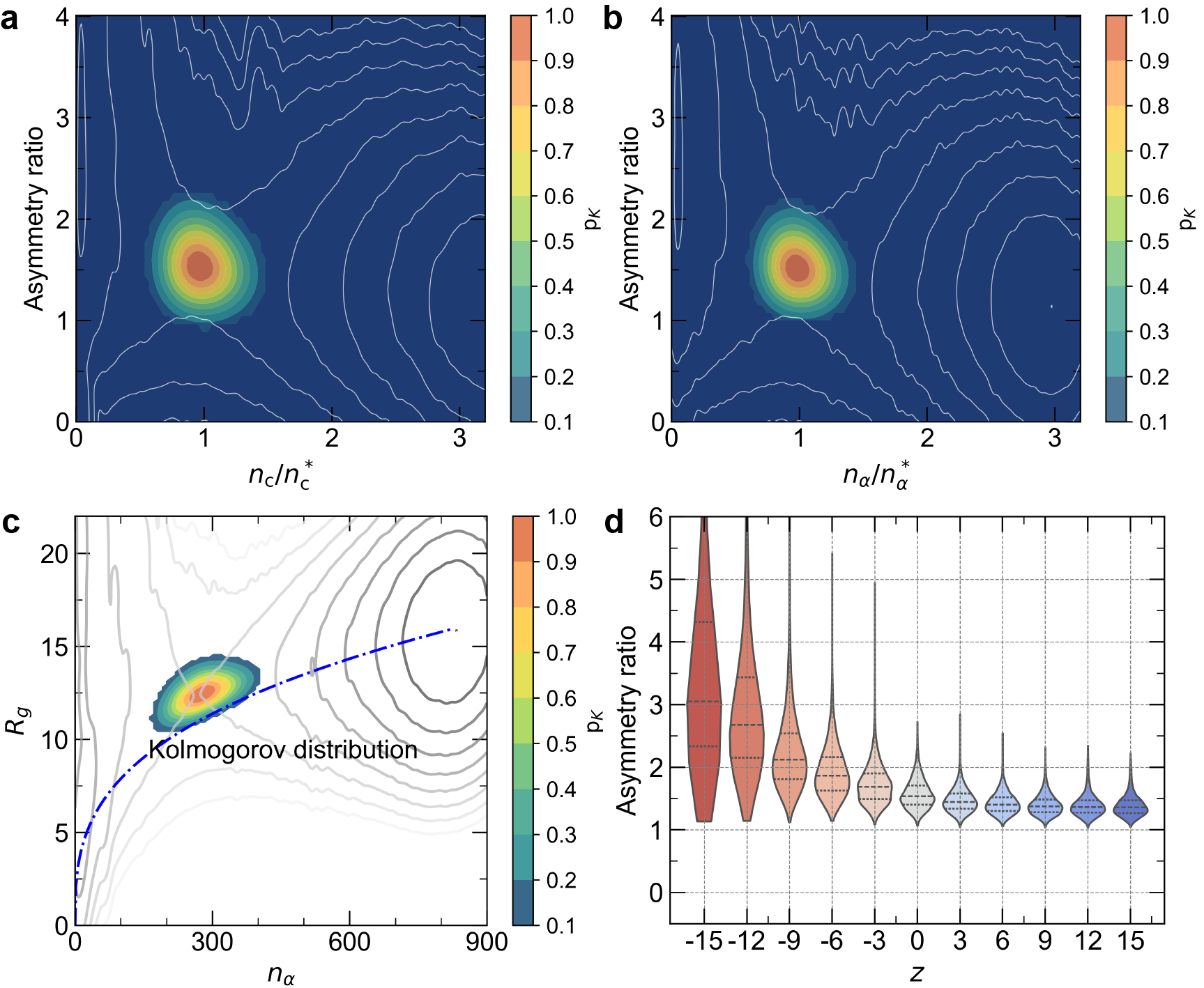
Figure S8: Kolmogorov distribution density in the plane of a) $n_{\text{c}}$ and asymmetry ratio and b) $n_{\alpha}$ and asymmetry ratio. The x coordinates are rescaled according to the values of their critical numbers, respectively. The white isolines represent the reference free energy levels. c) Kolmogorov distribution density in the $n_{\alpha}$-$R_{g}$ plane. The gray lines are free energy levels, while the blue dashed-dotted line shows the size-scaling relation $R_{g}\propto n_{\alpha}^{1/3}$ where the proportionality constant is fitted to state $B$. d) Violin plot of the distribution of asymmetry ratio of each bin along $z$.

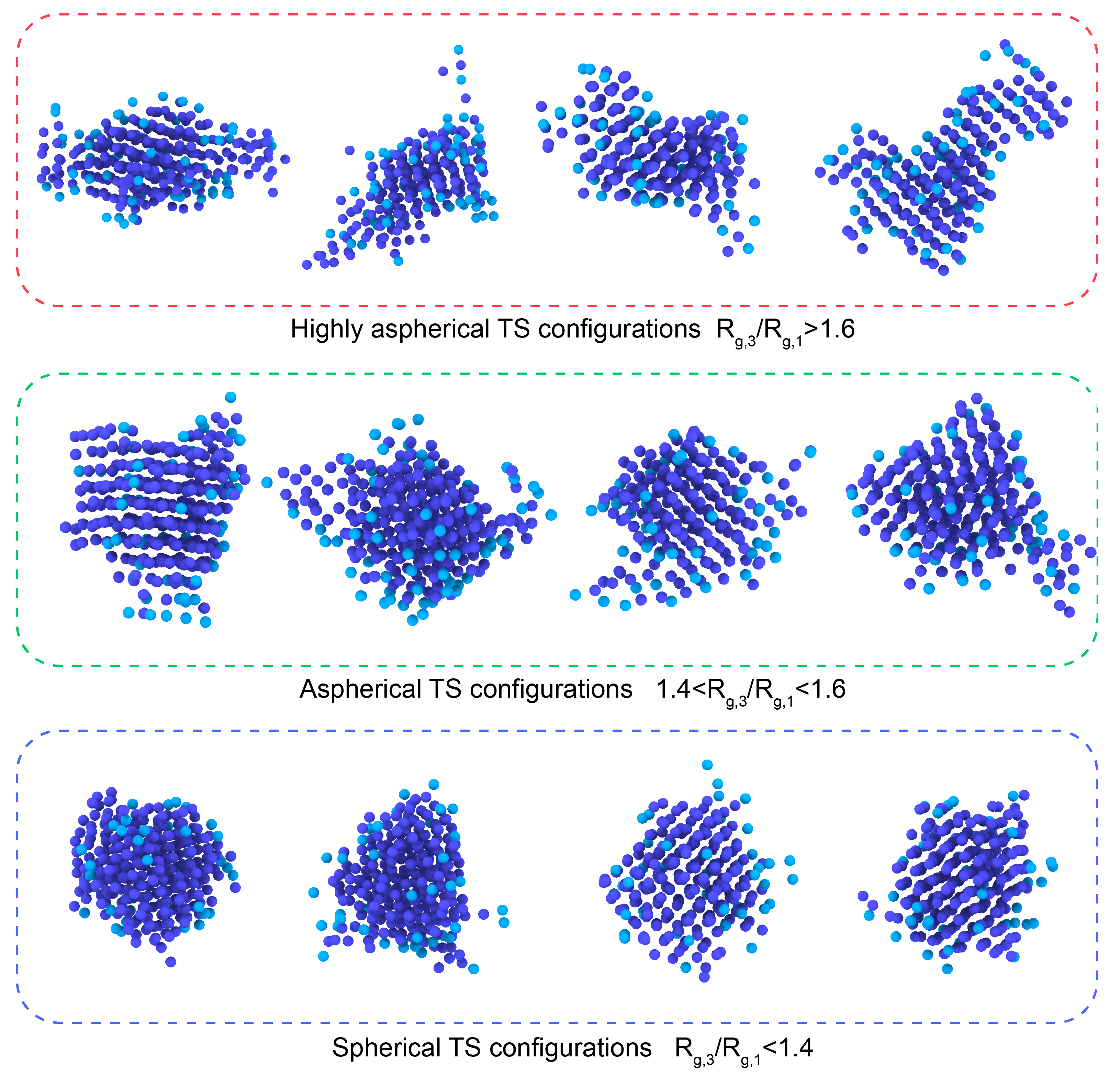
Figure S9: Snapshots of representative spherical, aspherical, and highly aspherical transition state (TS) configurations. Atoms forming the conventional $n_{\text{c}}$ nucleus are colored in blue, while the additional atoms included in the $n_{\alpha}$ definition are colored in cyan.

S5 Probability-based $n_{\alpha}$

We further validate $n_{\alpha}$ as a descriptor of the nucleation transition by correlating it with the committor probability and comparing it against convetional $n_{\text{c}}$. We project the committor function $q(\mathbf{x})$ and $z(\mathbf{x})$ onto both $n_{\text{c}}$ and $n_{\alpha}$ metrics. Fig. S10 shows that $n_{\alpha}$ exhibits fluctuations comparable to those of $n_{\text{c}}$, suggesting that both descriptors yield similar fluctuation levels. However, a balanced evaluation requires accounting for the number of atoms per bin under each criterion. To quantify their differences, we compute the normalized root mean square deviation (NRMSD) along each bin of $q$ and $z$. As shown in Fig. 4b and Fig. S11, the $\alpha>\frac{1}{2}$ criterion minimizes NRMSD when normalized by the average atom count per bin, while capturing more atoms surrounding the emerging nucleus at comparable fluctuation levels. This precision arises from $n_{\alpha}$’s probabilistic definition, which comprehensively includes all atoms in the solid-like peak, making it a more reliable and physically meaningful measure of nucleus size than $n_{\text{c}}$. To more clearly illustrate the effect of our probability-based $n_{\alpha}$, we highlight in Fig. S9 the atoms characterized by $n_{\text{c}}$ and those additionally included as part of the nucleus by $n_{\alpha}$ using distinct colors.

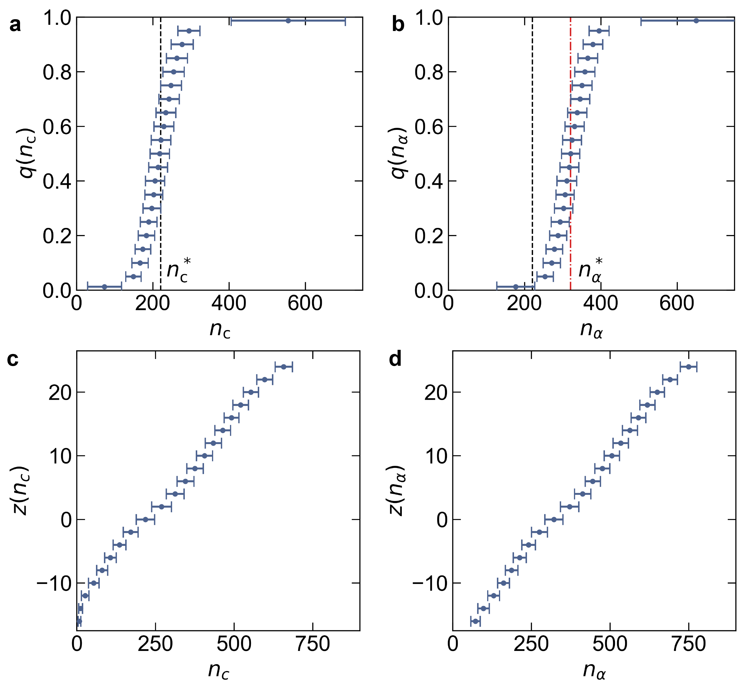
Figure S10: Projection of committor function $q$ as a function of a) $n_{\text{c}}$ and b) $n_{\alpha}$. Dashed lines referred to the critical nucleus size estimated from $q(n_{\text{c}}^{*})=0.5$, while the red dashed-dotted line referred to the critical nucleus size estimated from $q(n_{\alpha}^{*})=0.5$. Projection of $z$ as a function of c) $n_{\text{c}}$ and d) $n_{\alpha}$.

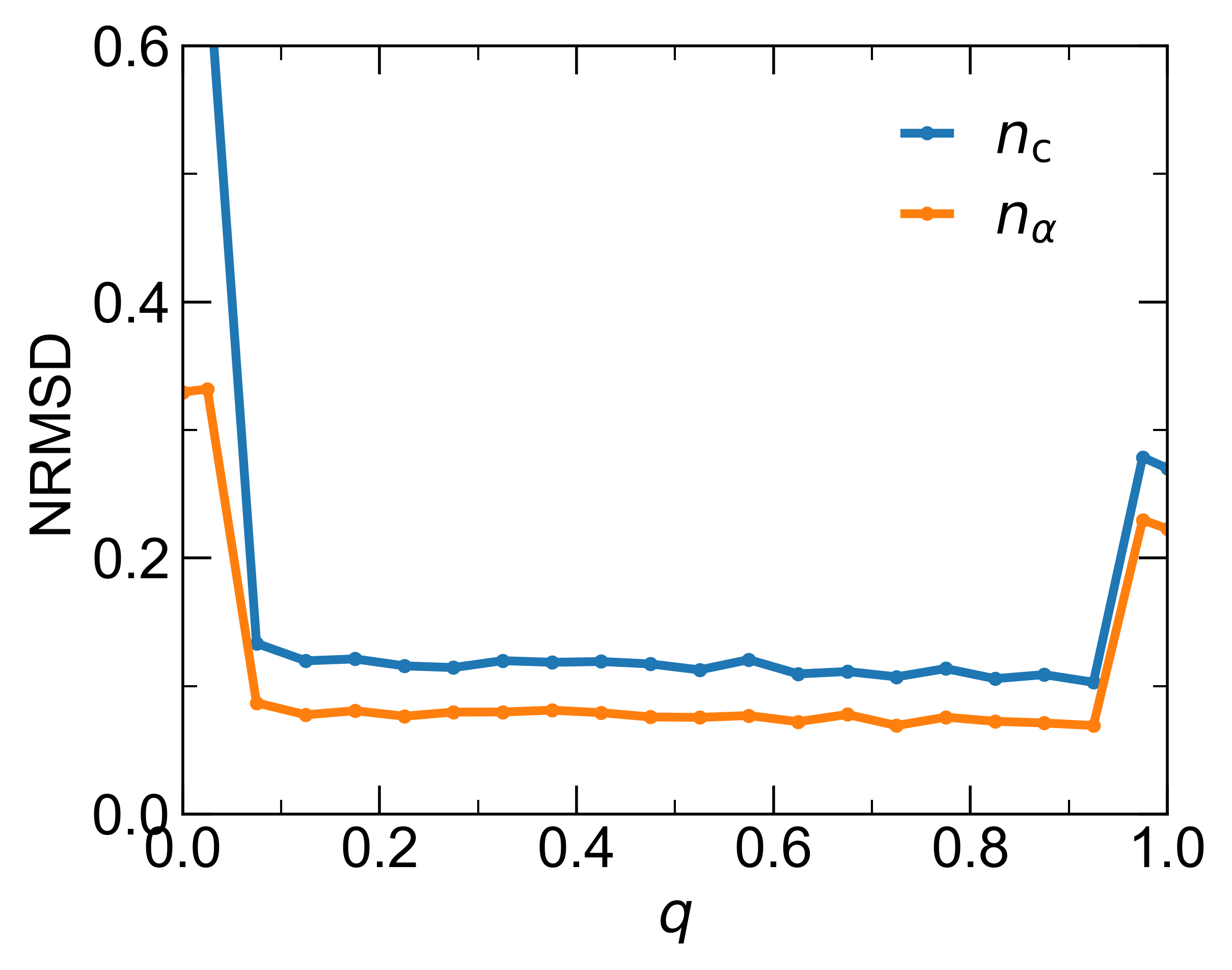
Figure S11: NRMSD of $n_{\text{c}}$ and $n_{\alpha}$ as functions of $q$.

S6 Estimation of nucleation rate

We first determine the self diffusion coefficient $D$ of the under cooled liquid with the mean square displacement (MSD), defined as:

$$D=\frac{\text{MSD}}{6t}\text{ , where }\text{MSD}=\frac{1}{N}\sum_{i=1}^{N}[\vec{r_{i}}(t)-\vec{r_{i}}(0)]^{2}$$ (S19)

where $\vec{r}_{i}(t)$ represents the position of particle $i$ at time $t$, and $N$ is the total number of particles. Next, we perform a number of overdamped Langevin dynamics simulations with varying friction coefficient $\gamma$. As shown in Fig. S12, we chose $\gamma^{-1}=5\,\text{ps}$ that best reproduces the diffusion coefficient of the under cooled liquid.

By fully exploring each metastable states reversibly, we achieve an optimal functional value of $\mathcal{K}_{m}\approx 2.45\times 10^{-20}\,\textup{~\AA }^{-2}(\text{g/mol})^{-1}$, leading to a reaction rate of $\nu=7.07\times 10^{-6}\,\text{s}^{-1}$ according to Eq.2. Furthermore, the rate $k_{A\to B}$ is expressed as,

$$k_{A\to B}=\frac{v_{R}}{\rho_{A}}$$ (S20)

where $\rho_{A}=\lim_{T\to+\infty}\frac{T_{A}}{T}$ is derived from the free energy difference in Fig. S7,

$$\frac{\rho_{A}}{\rho_{B}}=e^{-\beta\Delta G_{A-B}}$$ (S21)

Finally, the nucleation rate is calculated as $J=k_{A\to B}/V\approx 1.9\times 10^{30}\,\text{m}^{-3}\text{s}^{-1}$.

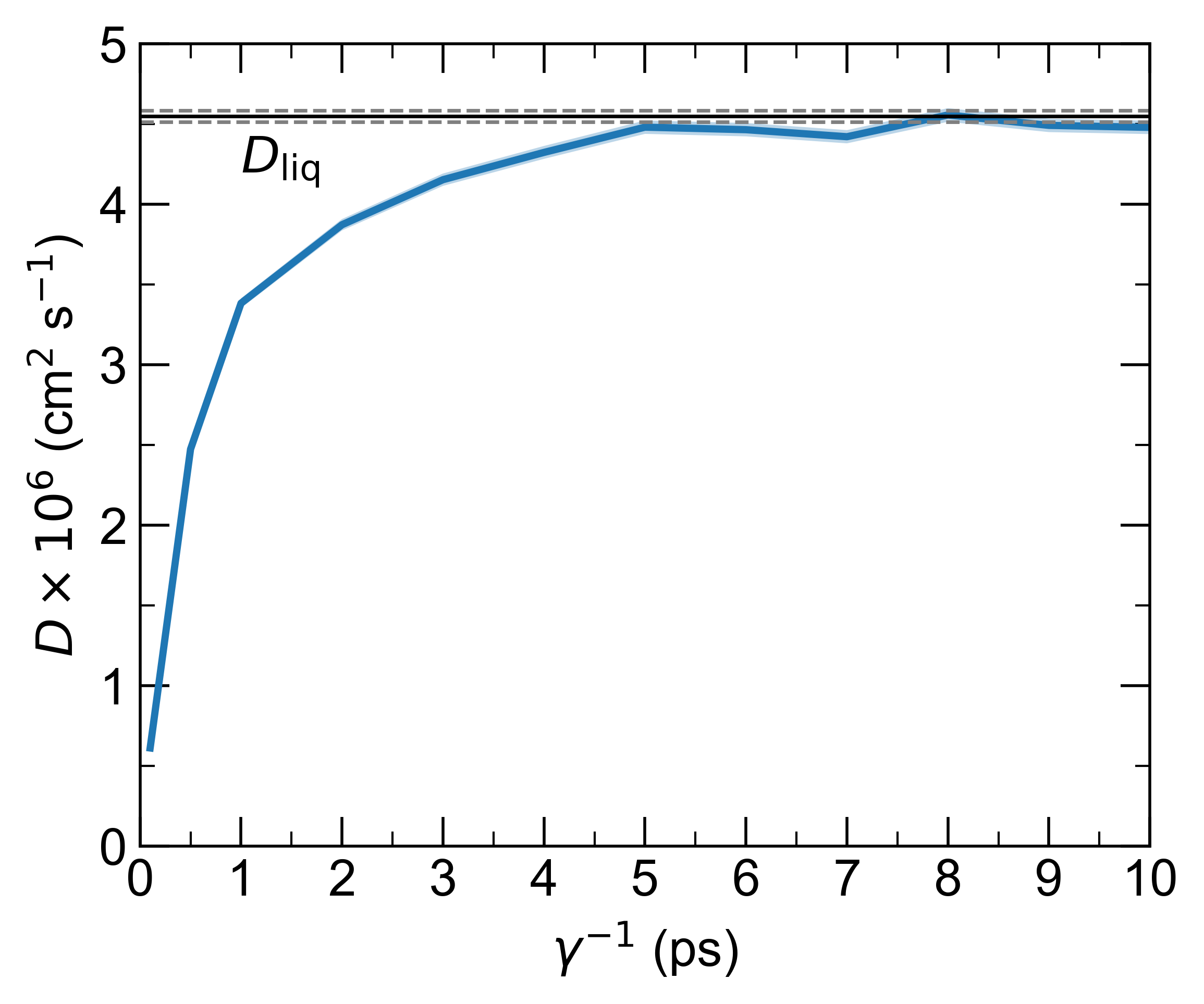
Figure S12: Diffusion coefficient $D$ as a function of $\gamma^{-1}$ from overdamped Langevin dynamics simulations of a 2916-atom LJ liquid. The diffusion coefficient $D_{\text{liq}}$ from Newtonian dynamics is represented by a dashed line as a reference.

Bibliography

- Kelton (1991) K. F. Kelton, “Crystal Nucleation in Liquids and Glasses,” in Solid State Physics, Vol. 45, edited by H. Ehrenreich and D. Turnbull (Academic Press, 1991) pp. 75–177.
- Oxtoby (1992) D. W. Oxtoby, “Homogeneous nucleation: theory and experiment,” Journal of Physics: Condensed Matter 4, 7627 (1992).
- Mandell, McTague, and Rahman (1977) M. J. Mandell, J. P. McTague, and A. Rahman, “Crystal nucleation in a three-dimensional Lennard-Jones system. II. Nucleation kinetics for 256 and 500 particles,” The Journal of Chemical Physics 66, 3070–3075 (1977).
- Stillinger and Weber (1978) F. H. Stillinger and T. A. Weber, “Study of melting and freezing in the Gaussian core model by molecular dynamics simulation,” The Journal of Chemical Physics 68, 3837–3844 (1978).
- Hsu and Rahman (1979) C. S. Hsu and A. Rahman, “Crystal nucleation and growth in liquid rubidium,” The Journal of Chemical Physics 70, 5234–5240 (1979).
- Giberti, Salvalaglio, and Parrinello (2015) F. Giberti, M. Salvalaglio, and M. Parrinello, “Metadynamics studies of crystal nucleation,” IUCrJ 2, 256–266 (2015).
- Sosso et al. (2016) G. C. Sosso, J. Chen, S. J. Cox, M. Fitzner, P. Pedevilla, A. Zen, and A. Michaelides, “Crystal Nucleation in Liquids: Open Questions and Future Challenges in Molecular Dynamics Simulations,” Chemical Reviews 116, 7078–7116 (2016).
- Finney and Salvalaglio (2024) A. R. Finney and M. Salvalaglio, “Molecular simulation approaches to study crystal nucleation from solutions: Theoretical considerations and computational challenges,” WIREs Computational Molecular Science 14, e1697 (2024).
- Torrie and Valleau (1977) G. M. Torrie and J. P. Valleau, “Nonphysical sampling distributions in Monte Carlo free-energy estimation: Umbrella sampling,” Journal of Computational Physics 23, 187–199 (1977).
- Laio and Parrinello (2002) A. Laio and M. Parrinello, “Escaping free-energy minima,” Proceedings of the National Academy of Sciences 99, 12562–12566 (2002).
- Invernizzi and Parrinello (2020) M. Invernizzi and M. Parrinello, “Rethinking Metadynamics: From Bias Potentials to Probability Distributions,” The Journal of Physical Chemistry Letters 11, 2731–2736 (2020).
- Invernizzi and Parrinello (2022) M. Invernizzi and M. Parrinello, “Exploration vs Convergence Speed in Adaptive-Bias Enhanced Sampling,” Journal of Chemical Theory and Computation 18, 3988–3996 (2022).
- Dellago et al. (1998) C. Dellago, P. G. Bolhuis, F. S. Csajka, and D. Chandler, “Transition path sampling and the calculation of rate constants,” The Journal of Chemical Physics 108, 1964–1977 (1998).
- Van Erp, Moroni, and Bolhuis (2003) T. S. Van Erp, D. Moroni, and P. G. Bolhuis, “A novel path sampling method for the calculation of rate constants,” The Journal of Chemical Physics 118, 7762–7774 (2003).
- Allen, Valeriani, and Rein Ten Wolde (2009) R. J. Allen, C. Valeriani, and P. Rein Ten Wolde, “Forward flux sampling for rare event simulations,” Journal of Physics: Condensed Matter 21, 463102 (2009).
- Espinosa et al. (2016) J. R. Espinosa, C. Vega, C. Valeriani, and E. Sanz, “Seeding approach to crystal nucleation,” The Journal of Chemical Physics 144, 034501 (2016).
- Rein Ten Wolde, Ruiz-Montero, and Frenkel (1996) P. Rein Ten Wolde, M. J. Ruiz-Montero, and D. Frenkel, “Numerical calculation of the rate of crystal nucleation in a Lennard-Jones system at moderate undercooling,” The Journal of Chemical Physics 104, 9932–9947 (1996).
- Moroni, Ten Wolde, and Bolhuis (2005) D. Moroni, P. R. Ten Wolde, and P. G. Bolhuis, “Interplay between Structure and Size in a Critical Crystal Nucleus,” Physical Review Letters 94, 235703 (2005).
- Trudu, Donadio, and Parrinello (2006) F. Trudu, D. Donadio, and M. Parrinello, “Freezing of a Lennard-Jones Fluid: From Nucleation to Spinodal Regime,” Physical Review Letters 97, 105701 (2006).
- Jungblut and Dellago (2011) S. Jungblut and C. Dellago, “Crystallization of a binary Lennard-Jones mixture,” The Journal of Chemical Physics 134, 104501 (2011).
- Kolmogoroff (1931) A. Kolmogoroff, “Über die analytischen Methoden in der Wahrscheinlichkeitsrechnung,” Mathematische Annalen 104, 415–458 (1931).
- E and Vanden-Eijnden (2010) W. E and E. Vanden-Eijnden, “Transition-Path Theory and Path-Finding Algorithms for the Study of Rare Events,” Annual Review of Physical Chemistry 61, 391–420 (2010).
- Berezhkovskii and Szabo (2005) A. Berezhkovskii and A. Szabo, “One-dimensional reaction coordinates for diffusive activated rate processes in many dimensions,” The Journal of Chemical Physics 122, 014503 (2005).
- Ma and Dinner (2005) A. Ma and A. R. Dinner, “Automatic Method for Identifying Reaction Coordinates in Complex Systems,” The Journal of Physical Chemistry B 109, 6769–6779 (2005).
- Li and Ma (2014) W. Li and A. Ma, “Recent developments in methods for identifying reaction coordinates,” Molecular Simulation 40, 784–793 (2014).
- He, Chipot, and Roux (2022) Z. He, C. Chipot, and B. Roux, “Committor-Consistent Variational String Method,” The Journal of Physical Chemistry Letters 13, 9263–9271 (2022).
- Lazzeri et al. (2023) G. Lazzeri, H. Jung, P. G. Bolhuis, and R. Covino, “Molecular Free Energies, Rates, and Mechanisms from Data-Efficient Path Sampling Simulations,” Journal of Chemical Theory and Computation 19, 9060–9076 (2023).
- Vanden-Eijnden and Tal (2005) E. Vanden-Eijnden and F. A. Tal, “Transition state theory: Variational formulation, dynamical corrections, and error estimates,” The Journal of Chemical Physics 123, 184103 (2005).
- Maragliano and Vanden-Eijnden (2006) L. Maragliano and E. Vanden-Eijnden, “A temperature accelerated method for sampling free energy and determining reaction pathways in rare events simulations,” Chemical Physics Letters 426, 168–175 (2006).
- Zinovjev and Tuñón (2015) K. Zinovjev and I. Tuñón, “Transition state ensemble optimization for reactions of arbitrary complexity,” The Journal of Chemical Physics 143, 134111 (2015).
- Khoo, Lu, and Ying (2019) Y. Khoo, J. Lu, and L. Ying, “Solving for high-dimensional committor functions using artificial neural networks,” Research in the Mathematical Sciences 6, 1–13 (2019).
- Li, Lin, and Ren (2019) Q. Li, B. Lin, and W. Ren, “Computing committor functions for the study of rare events using deep learning,” The Journal of Chemical Physics 151 (2019).
- Kang, Trizio, and Parrinello (2024) P. Kang, E. Trizio, and M. Parrinello, “Computing the committor with the committor to study the transition state ensemble,” Nature Computational Science 4, 451–460 (2024).
- Trizio, Kang, and Parrinello (2024) E. Trizio, P. Kang, and M. Parrinello, “Everything everywhere all at once, a probability-based enhanced sampling approach to rare events,” (2024).
- Piaggi, Valsson, and Parrinello (2017) P. M. Piaggi, O. Valsson, and M. Parrinello, “Enhancing Entropy and Enthalpy Fluctuations to Drive Crystallization in Atomistic Simulations,” Physical Review Letters 119, 015701 (2017).
- Niu, Yang, and Parrinello (2019) H. Niu, Y. I. Yang, and M. Parrinello, “Temperature Dependence of Homogeneous Nucleation in Ice,” Physical Review Letters 122, 245501 (2019).
- Deng, Du, and Li (2021) Y. Deng, T. Du, and H. Li, “Relationship of structure and mechanical property of silica with enhanced sampling and machine learning,” Journal of the American Ceramic Society 104, 3910–3920 (2021).
- Karmakar et al. (2021) T. Karmakar, M. Invernizzi, V. Rizzi, and M. Parrinello, “Collective variables for the study of crystallisation,” Molecular Physics , e1893848 (2021).
- Deng et al. (2023) Y. Deng, S. Fu, J. Guo, X. Xu, and H. Li, “Anisotropic Collective Variables with Machine Learning Potential for Ab Initio Crystallization of Complex Ceramics,” ACS Nano 17, 14099–14113 (2023).
- Jung et al. (2023) H. Jung, R. Covino, A. Arjun, C. Leitold, C. Dellago, P. G. Bolhuis, and G. Hummer, “Machine-guided path sampling to discover mechanisms of molecular self-organization,” Nature Computational Science 3, 334–345 (2023).
- Steinhardt, Nelson, and Ronchetti (1983) P. J. Steinhardt, D. R. Nelson, and M. Ronchetti, “Bond-orientational order in liquids and glasses,” Physical Review B 28, 784–805 (1983).
- Piaggi and Parrinello (2017) P. M. Piaggi and M. Parrinello, “Entropy based fingerprint for local crystalline order,” The Journal of Chemical Physics 147, 114112 (2017).
- E, Ren, and Vanden-Eijnden (2002) W. E, W. Ren, and E. Vanden-Eijnden, “String method for the study of rare events,” Physical Review B 66, 052301 (2002).
- Binder (1995) K. Binder, Monte Carlo and Molecular Dynamics Simulations in Polymer Science (Oxford University Press, 1995).
- Möller et al. (2024) J. Möller, A. Schottelius, M. Caresana, U. Boesenberg, C. Kim, F. Dallari, T. A. Ezquerra, J. M. Fernández, L. Gelisio, A. Glaesener, C. Goy, J. Hallmann, A. Kalinin, R. P. Kurta, D. Lapkin, F. Lehmkühler, F. Mambretti, M. Scholz, R. Shayduk, F. Trinter, I. A. Vartaniants, A. Zozulya, D. E. Galli, G. Grübel, A. Madsen, F. Caupin, and R. E. Grisenti, “Crystal Nucleation in Supercooled Atomic Liquids,” Physical Review Letters 132, 206102 (2024).
- Tipeev, Zanotto, and Rino (2018) A. O. Tipeev, E. D. Zanotto, and J. P. Rino, “Diffusivity, Interfacial Free Energy, and Crystal Nucleation in a Supercooled Lennard-Jones Liquid,” The Journal of Physical Chemistry C 122, 28884–28894 (2018).
- Das et al. (2024) S. Das, U. Raucci, R. P. P. Neves, M. J. Ramos, and M. Parrinello, “Correlating enzymatic reactivity for different substrates using transferable data-driven collective variables,” Proceedings of the National Academy of Sciences 121, e2416621121 (2024).
- Paszke et al. (2019) A. Paszke, S. Gross, F. Massa, A. Lerer, J. Bradbury, G. Chanan, T. Killeen, Z. Lin, N. Gimelshein, L. Antiga, A. Desmaison, A. Köpf, E. Yang, Z. DeVito, M. Raison, A. Tejani, S. Chilamkurthy, B. Steiner, L. Fang, J. Bai, and S. Chintala, “PyTorch: An Imperative Style, High-Performance Deep Learning Library,” (2019).
- Bonati et al. (2023) L. Bonati, E. Trizio, A. Rizzi, and M. Parrinello, “A unified framework for machine learning collective variables for enhanced sampling simulations: mlcolvar,” The Journal of Chemical Physics 159, 014801 (2023).
- Thompson et al. (2022) A. P. Thompson, H. M. Aktulga, R. Berger, D. S. Bolintineanu, W. M. Brown, P. S. Crozier, P. J. In ’T Veld, A. Kohlmeyer, S. G. Moore, T. D. Nguyen, R. Shan, M. J. Stevens, J. Tranchida, C. Trott, and S. J. Plimpton, “LAMMPS - a flexible simulation tool for particle-based materials modeling at the atomic, meso, and continuum scales,” Computer Physics Communications 271, 108171 (2022).
- Tribello et al. (2014) G. A. Tribello, M. Bonomi, D. Branduardi, C. Camilloni, and G. Bussi, “PLUMED 2: New feathers for an old bird,” Computer Physics Communications 185, 604–613 (2014).
- Stukowski (2010) A. Stukowski, “Visualization and analysis of atomistic simulation data with OVITO–the Open Visualization Tool,” Modelling and Simulation in Materials Science and Engineering 18, 015012 (2010).
- Lechner and Dellago (2008) W. Lechner and C. Dellago, “Accurate determination of crystal structures based on averaged local bond order parameters,” The Journal of Chemical Physics 129, 114707 (2008).
- Bonomi, Barducci, and Parrinello (2009) M. Bonomi, A. Barducci, and M. Parrinello, “Reconstructing the equilibrium Boltzmann distribution from well-tempered metadynamics,” Journal of Computational Chemistry 30, 1615–1621 (2009).
- Rowley, Nicholson, and Parsonage (1975) L. Rowley, D. Nicholson, and N. Parsonage, “Monte Carlo grand canonical ensemble calculation in a gas-liquid transition region for 12-6 Argon,” Journal of Computational Physics 17, 401–414 (1975).
- Sun (1998) H. Sun, “COMPASS: An ab Initio Force-Field Optimized for Condensed-Phase ApplicationsOverview with Details on Alkane and Benzene Compounds,” The Journal of Physical Chemistry B 102, 7338–7364 (1998).
- Hoover (1985) W. G. Hoover, “Canonical dynamics: Equilibrium phase-space distributions,” Physical Review A 31, 1695–1697 (1985).
- Parrinello and Rahman (1981) M. Parrinello and A. Rahman, “Polymorphic transitions in single crystals: A new molecular dynamics method,” Journal of Applied Physics 52, 7182–7190 (1981).
- Mastny and De Pablo (2007) E. A. Mastny and J. J. De Pablo, “Melting line of the Lennard-Jones system, infinite size, and full potential,” The Journal of Chemical Physics 127, 104504 (2007).