Fast relaxation of a viscous vortex in an external flow
Martin Donati and Thierry Gallay
(April 5, 2025)
Abstract
We study the evolution of a concentrated vortex advected by a smooth, divergence-free velocity field in two space dimensions. In the idealized situation where
the initial vorticity is a Dirac mass, we compute an approximation of the
solution which accurately describes, in the regime of high Reynolds numbers, the
motion of the vortex center and the deformation of the streamlines under the
shear stress of the external flow. For ill-prepared initial data, corresponding
to a sharply peaked Gaussian vortex, we prove relaxation to the previous
solution on a time scale that is much shorter than the diffusive time, due to
enhanced dissipation inside the vortex core.
1 Introduction
We revisit the classical problem of the evolution of a concentrated vortex in a
background flow, which was carefully studied in the monographs [24, 25]
and the previous works [26, 14]. We assume that the external velocity
field is smooth, divergence-free, and uniformly bounded together with its
derivatives. Our goal is to give a rigorous description of the solution of the
two-dimensional Navier-Stokes equations in such a background flow, for
concentrated initial data corresponding either to a point vortex or to a sharply
peaked Gaussian vortex. In both cases the solution remains concentrated for
quite a long time provided the kinematic viscosity is sufficiently
small. The leading order approximation is a Lamb-Oseen vortex whose center is
advected by the external flow, whereas the vortex core spreads diffusively due
to viscosity. Higher order corrections describe the deformation of the
streamlines under the external shear stress, and appear to be sensitive to the
choice of the initial data.
From the point of view of mathematical analysis, it is convenient to consider
first the idealized situation where the initial vorticity is just a Dirac mass.
Despite the singular nature of such data, the initial value problem remains
globally well-posed, as can be seen by adapting to the present case the
results that are known for the two-dimensional vorticity equation in the space
of finite measures [11, 8, 10]. By construction, the size of the
vortex core vanishes at initial time, and is therefore infinitely small compared
to the typical length scale defined by the external flow. For such
well-prepared initial data, the approximate solution constructed in
[26, 24] depends only on the “normal” time scale associated with
the external field, and describes the deformation of the vortex core under
the external shear stress.
The situation is quite different if the initial vorticity is a radially
symmetric vortex patch or vortex blob with finite extension . Such data can be described as ill-prepared, in the sense that the
resulting solution exhibits a transient regime during which the initially
symmetric vortex gets deformed to adapt its shape to the external strain. The
streamlines near the vortex core become elliptical, with an eccentricity that
undergoes damped oscillations on a short time scale until it settles down to the
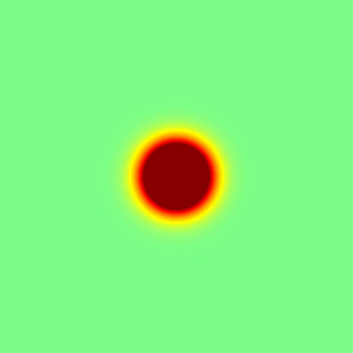
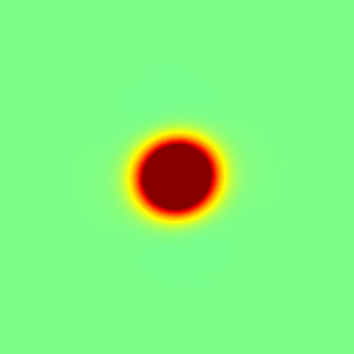
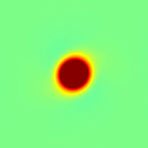
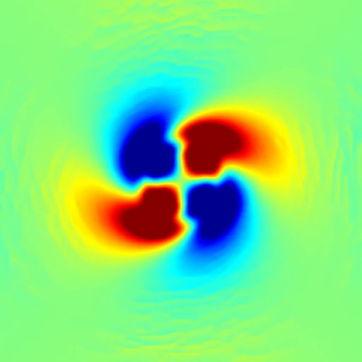
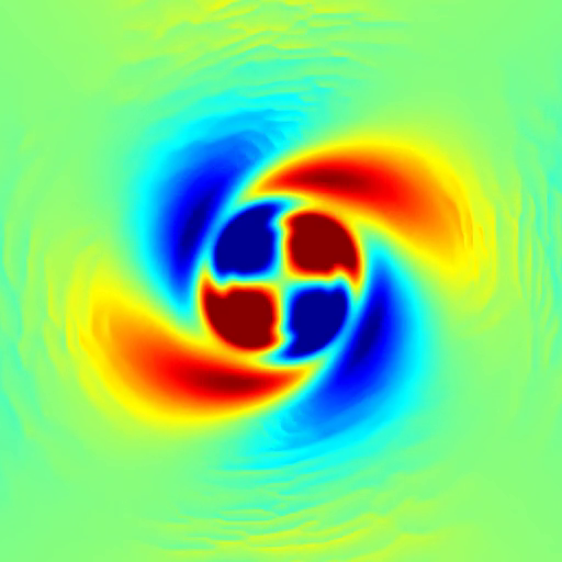
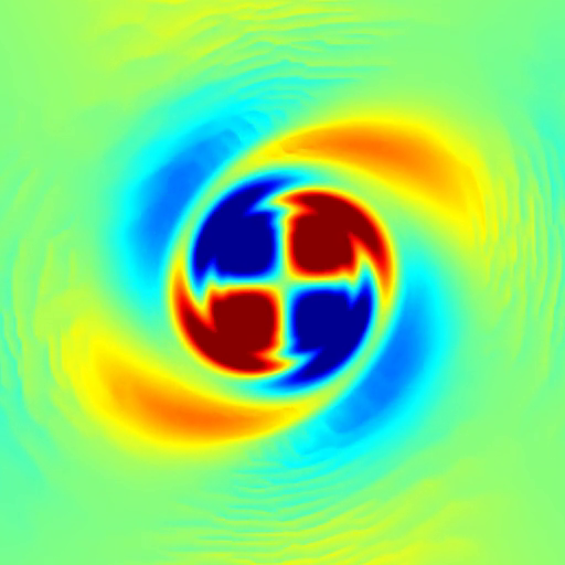
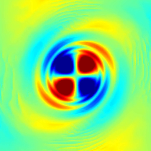
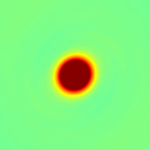
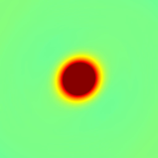
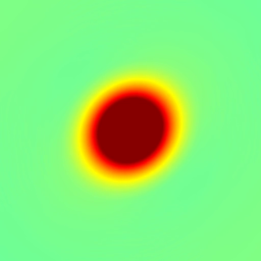
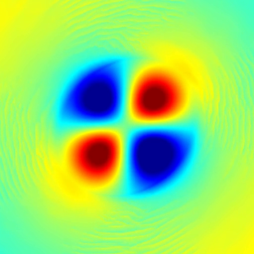
value predicted by the well-prepared solution. This evolution is illustrated by a
numerical simulation in Figure 1. In a second stage, the vorticity
distribution inside the core slowly relaxes to a Gaussian profile under the
action of viscosity. This two-step process was carefully studied by Le Dizès
and Verga [12] in the related case of a co-rotating vortex pair, for
which the deformation of the vortex cores is just the first stage of a complex
dynamics eventually leading to vortex merging [21]. In the
perturbative approach of Ting and Klein [24], a two-time analysis is
necessary to obtain an accurate description of the solution in the ill-prepared
case.
()
()
()
()
()
()
()
()
()
()
()
()
()
()
()
()
()
()
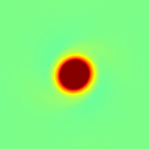
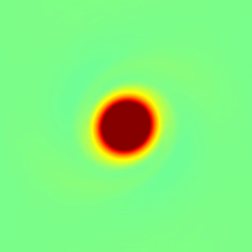
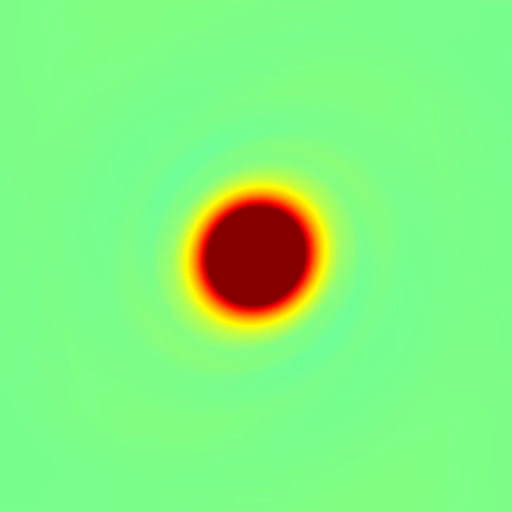
Figure 1: Numerical simulation of a vortex in an external field with Gaussian initial data.
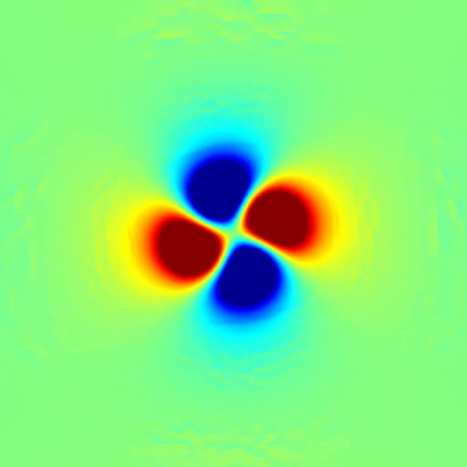
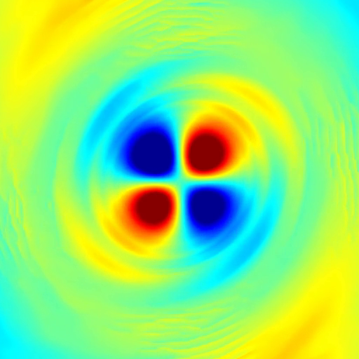
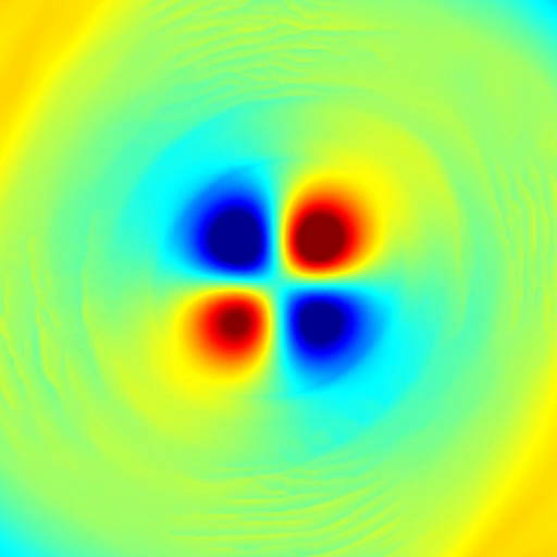
The vorticity distribution (left) and the deviation from the Lamb-Oseen vortex (right)
are represented at nine different times, using standard color codes for the vorticity
levels. The final state at is close to the approximate solution defined
in (1.10). This simulation is made with the free software
Basilisk, and the external field is chosen as
in Appendix A.1.
The purpose of this paper is twofold. First, we show that the techniques
introduced in [4] to study the solution of the two-dimensional
Navier-Stokes equations with a finite collection of point vortices as initial
data can be adapted to the emblematic case of a single vortex in an external
flow, which is at the same time simpler and more general. In particular, if the
initial vorticity is a Dirac mass, we construct perturbatively an accurate
approximation of the solution, and we verify that the exact solution remains
close to it over a long time interval if the viscosity is small enough. Next, we
consider ill-prepared data for which the initial vorticity is a sharply
concentrated Gaussian function, and we prove that the resulting solution rapidly
relaxes towards the approximate solution computed in the well-prepared case.
That part of the analysis relies on enhanced dissipation estimates for the
linearized Navier-Stokes equations at the Lamb-Oseen vortex, which are due to
Li, Wei, and Zhang [13]. Such estimates were already applied in
[5] to quantify the stability properties of a Gaussian vortex in the
regime of high Reynolds numbers, but to our knowledge they were never used to
study the deformation of vortices under external strain.
We now present our results in a more precise way. We give ourselves a
smooth, time-dependent velocity field
which is uniformly bounded together with its derivatives with respect to the space
variable and the time . We assume that
is divergence-free, namely
The characteristic time of the velocity field is defined by
the classical formula
(1.1)
where denotes the first order differential of with respect to the
space variable. To avoid trivial situations, we suppose from now on that
, which means that .
We consider the evolution of a concentrated vortex embedded
in the external flow described by the velocity field . The vorticity
distribution is a scalar function satisfying the evolution equation
(1.2)
where the parameter is the kinematic viscosity of the the fluid.
The velocity field associated with is given by the
Biot-Savart formula
(1.3)
where we use the notation and for
all . We denote and we observe that
and .
Equations (1.2), (1.3) form a closed system, which corresponds
when to the usual two-dimensional incompressible Navier-Stokes
equations in vorticity form. We refer the reader to [18, 20] for
general results on these equations.
Remark 1.1.
Equation (1.2) appears in at least two physical contexts. The first
one is the evolution of a finite number of isolated vortices under the dynamics
of the Navier-Stokes equations in . A natural strategy in this situation
is to concentrate on the motion of one particular vortex, in which case the
corresponding vorticity distribution satisfies the evolution equation
(1.2) with and being the velocity field
associated with all the other vortices in the flow, see for example
[19, 10, 4]. Note that the vorticity is advected by the velocity field , so that the
external flow is not independent of the solution of (1.2).
Alternatively, following [24, 25], we can consider the evolution of a
single vortex in a background potential flow , which is typically due to
an inflow condition at infinity. In that case , so that the
dynamics of the vortex does not influence the external flow.
We first consider the idealized situation where the initial vorticity is a
Dirac mass, which means that for some
and some . Without loss of generality, we assume henceforth that
. Adapting the results of [11, 10], which hold
for , it is not difficult to verify that Eq. (1.2) has a unique
(mild) solution such that
(1.4)
where the half-arrow denotes the weak convergence of measures.
In the simple case where , the solution takes the explicit form
(1.5)
for all , where the vorticity and the
velocity are given by
(1.6)
Note that , so that actually solves
the linear heat equation . The self-similar
solution (1.5) of the two-dimensional vorticity equation is referred
to as the Lamb-Oseen vortex with circulation , centered at the point
. More generally, for solutions of (1.2), (1.3),
the total circulation is the conserved quantity defined by
The dimensionless ratio is called the circulation Reynolds number.
In the more interesting situation where , no explicit expression
is available in general, but if the viscosity is weak enough so that the
diffusion length is small compared to the characteristic length
defined by the external flow, we can approximate the solution of (1.2)
by a sharply concentrated Lamb-Oseen vortex which is simply advected by the
external velocity field. This fact is rigorously stated in the following result.
Proposition 1.2.
Fix and . There exist positive constants
such that, if , the unique solution of (1.2),
(1.3) satisfying (1.4) has the following property:
(1.7)
where and is the unique solution of the
differential equation
(1.8)
Remark 1.3.
The dimensionless constants depend only on the ratio
and on the quantity
(1.9)
which measures the intensity of the external flow. We expect that
and as or . We emphasize, however, that estimate (1.7) holds uniformly in
provided the inverse Reynolds number is sufficiently
small. In particular we see that
for all as .
Remark 1.4.
The quantity can be interpreted as the effective size of
a vortex of circulation in an external field, namely the size of the
neighborhood of the vortex center in which the external strain is weaker than
the strain of the vortex itself. It should not be confused with the size of the vortex
core, which depends on the vorticity distribution and can be considerably smaller.
In the setting of Proposition 1.2, the latter quantity is proportional to the
diffusion length , which is indeed much smaller than if
. Under these assumptions, estimate (1.7)
provides a good approximation of the solution of (1.2).
Estimate (1.7) is simple and elegant, but does not describe the
deformation of the vortex core under the action of the external flow, which is
the main phenomenon we want to study in this paper. Therefore we need a more
precise asymptotic expansion of the solution of (1.2), which includes
non-radially symmetric corrections that were neglected in (1.7).
To this end, we propose the following approximation of a Gaussian vortex of
circulation and core size , located at a point
, and undergoing the strain of an external velocity field :
(1.10)
Here, for all , we denote by the polar angle of the
rescaled variable , which is adapted to the description of the
vortex core. The strain rates are defined by
(1.11)
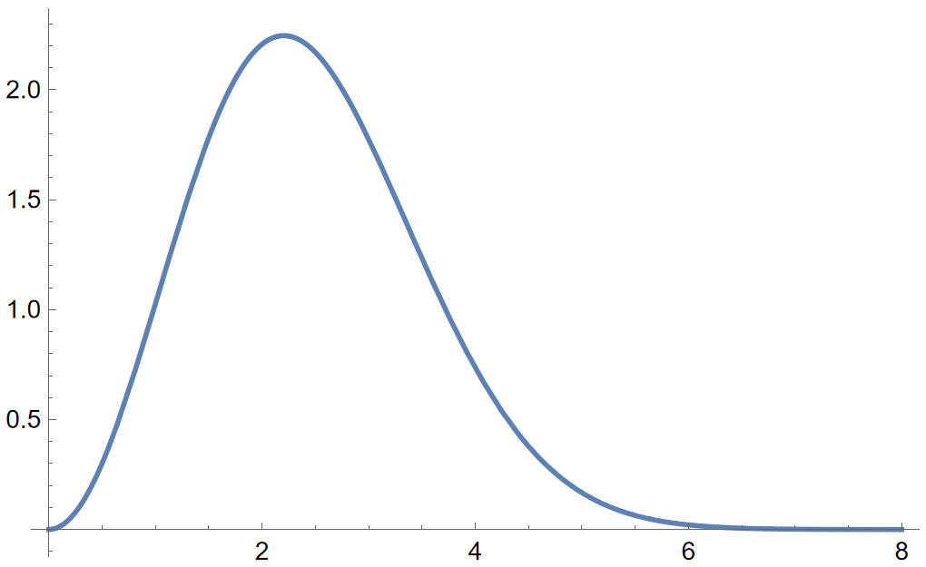
and the smooth function can be expressed
in terms of the solution of a linear differential equation, see
Remark 2.7 and Figure 2. For our purposes it is enough
to know that as and as
.
Remark 1.5.
The expression (1.10) is not new and appears in related contexts,
in particular in the large-Reynolds-number expansion of Burgers vortices,
see [23, 22] and Section A.1 below.
Identifying the core size with the diffusion length , we see
that the first term in the right-hand side of (1.10) is the
exactly Lamb-Oseen vortex (1.5), which is a radially symmetric
function of the rescaled variable ; in contrast, the correction term
involving depends explicitly on the polar angle . In view of
(1.1) the strain rates (1.11) are bounded by , so that
(1.12)
for some constant . If , as
is the case under the assumptions of Proposition 1.2, we deduce
that the Lamb-Oseen vortex is the leading term in the approximation
(1.10). We also observe that, since the correction term is a
linear function of and , the streamlines of the
corresponding velocity field are elliptical in a first approximation, which is of
course a well-known fact [12, 21].
We are now in a position to state our first main result, which subsumes Proposition 1.2.
Theorem 1.6.
Fix and . There exist positive constants
such that, if , the unique solution of (1.2),
(1.3) satisfying (1.4) has the following property:
(1.13)
where , , ,
and is the unique solution of the ODE
(1.14)
with initial condition .
Estimate (1.13) shows that the solution of (1.2) stays very
close to the approximation (1.10) with and
, provided the vortex position evolves according to the
ODE (1.14), which contains the viscous correction term
. We observe that, if the external velocity field is
irrotational, then so that
(1.14) reduces to (1.8). In the general case, the
solutions of (1.8), (1.14) do not coincide, but
they stay close to each other, and a simple calculation that is postponed
to Section 3.3.4 shows that estimate (1.13) implies
(1.7).
Remark 1.7.
The most natural way of locating the position of a concentrated vortex with
nonzero circulation is to use the center of vorticity ,
which satisfies
(1.15)
Under the assumptions of Theorem 1.6, we show in Section 3.3.4
that for some
constant . This means that the motion of the center of vorticity is
accurately described by the ODE (1.14), and that estimate (1.13)
still holds if is replaced by . In contrast, using the
approximate vortex position leads to a less precise control on
the solution, as in (1.7).
We now consider the different situation where the initial vorticity
is not a Dirac mass, but a Gaussian vortex of circulation and
small characteristic length . To facilitate the comparison with
the previous results, it is convenient to fix an initial time and
to assume that . Our second main result can be stated
as follows.
Theorem 1.8.
Fix , , and . There exist positive
constants such that, if , the unique
solution of (1.2), (1.3) with initial data
(1.16)
satisfies, for all , the estimate
(1.17)
where , , ,
, and is the unique solution of the ODE (1.14)
with initial condition .
Remark 1.9.
It is important to realize that the left-hand side of (1.17) does not
vanish at initial time , unless the strain rates and
are both equal to zero. Indeed, it follows from
(1.10), (1.16) that
and the norm of the right-hand side is proportional to .
In that sense our initial data (1.16) are ill-prepared if :
being radially symmetric around the point , they do not take into account the strain
of the external velocity field .
Since we have when
, where
for some . The right-hand side of (1.17) is therefore of
size as soon as
. In other words, the solution of (1.2)
rapidly relaxes towards the approximate solution (1.10),
which takes into account the effect of the external strain, and remains close to
it up to the final time . This description agrees with the numerical observation
in Figure 1. That the relaxation rate depends on the
inverse Reynolds number is a consequence of the enhanced dissipation effect in the vortex core, see [5] and
Section 4.
Theorem 1.8 can be seen as an extension of Theorem 1.6, in the sense
that the latter is obtained from the former by taking, at least formally, the
the limit . This connection can be made rigorous if we write the
the approximation formula (1.17) in a slightly more precise form,
see Section 4. The comparison of (1.13), (1.17) also
shows that the solution starting from a Dirac mass can be considered as a
canonical model for the deformation of a concentrated vortex in an
external field, in the sense that it attracts solutions of (1.2)
starting from ill-prepared initial data.
Remark 1.10.
In the context of Theorem 1.8, it is perfectly natural to start with a
radially symmetric vortex, but a priori there is no reason to restrict oneself
to the Gaussian case. As a matter of fact, numerical experiments show that
relaxation to the well-prepared solution occurs for a large class of initial
profiles, even though the damped oscillations that are observed in the transient
period after initial time strongly depend on the choice of the profile
[12]. In this paper we consider the particular initial data (1.16)
because we want to use the enhanced dissipation estimates of [13], which have
been established so far only in the Gaussian case.
The proof of our results relies on the construction of an approximate solution
of the initial value problem in self-similar variables, which is carried out in
Section 2. This part of the argument closely follows the previous works
[4, 3] where particular situations were considered. The proof of
Theorem 1.6 is carried out in Section 3, first under the
simplifying assumption that , and then for any . In both
cases the desired control on the solution is obtained by an energy estimate in
some weighted space, but the construction of the weight function is much
more complicated if is not small compared to . Improving upon the
results of [4], we construct a Gaussian-like weight that provides
an optimal control on the solution as far as the decay at infinity is
concerned, and implies in particular the estimate (1.13).
In Section 4, we show how these arguments can be combined with
the enhanced dissipation estimates obtained by Li, Wei, and Zhang [13]
to yield a proof of Theorem 1.8. Finally, a few auxiliary results
are collected in the Appendix. In particular, we clarify the link between our
approximate solution (1.10) and the Burgers vortex in an asymmetric
strain, and we investigate the motion of the center of vorticity under the
assumptions of Theorem 1.6.
2 Self-similar variables and approximate solution
We first explain the common strategy in the proofs of Theorems 1.6
and 1.8. Fix , , and let
be the solution of (1.2), (1.3) satisfying either
(1.4) or (1.16). In both cases, the solution
is sharply concentrated near a time-dependent point
if the viscosity is sufficiently small. To desingularize the
problem, it is useful to make the self-similar change of coordinates
(2.1)
In what follows we denote
(2.2)
The new space variable measures the distance to the vortex center
in units of the diffusion length . As already
explained, the small parameter is the inverse Reynolds number,
and the time-dependent aspect ratio compares the size
of the vortex core to the effective size of the
vortex.
As is easily verified, the evolution equation satisfied by the
rescaled vorticity is
(2.3)
where is the diffusion operator defined by
(2.4)
The position of the vortex center is unknown at this stage, but will be
chosen so as to minimize the quantity in
an appropriate sense. The leading order approximation corresponds to the natural
choice , but higher order corrections, leading to the
modified ODE (1.14), will be needed to achieve the desired
precision. We also observe that the rescaled velocity is divergence-free and satisfies , which means that
is obtained from by the Biot-Savart formula (1.3),
namely .
It is important to observe that (2.3) is not a regular
evolution equation at time , due to the singular time derivative
in the left-hand side. Nevertheless, if we adapt to the
present case the results of [8, 10], which hold for and
, it is not difficult to show that (2.3) has a unique
(mild) solution that
satisfies as .
This is precisely the solution we study in Theorem 1.6. Note that
the Gaussian profile (1.5) is, up to normalization, the only
possible choice for the initial vorticity at time . The situation
considered in Theorem 1.8 is much different: the Cauchy problem
for equation (2.3) is well-posed at any positive positive
time , and we could therefore choose arbitrary initial data at
. However, for reasons that are explained in Remark 1.10
above, our choice is to take the same initial vorticity as
in Theorem 1.6.
Since and is fixed, it is clear that the
evolution equation (2.3) becomes highly singular in the vanishing
viscosity limit , and this is actually the main problem in the
proof of both Theorems 1.6 and 1.8. To overcome this
difficulty, we use the approach introduced in [4, 6, 3]
which relies on the construction of an approximate solution of the form:
(2.5)
where . The vorticity profiles
and the velocity profiles depend on the small parameter
, and will be determined so that equality (2.3) holds
up to corrections terms of size .
Remark 2.1.
It is not obvious at this point that the aspect ratio
is the correct parameter for our perturbative expansion, since
it does not appear explicitly in the evolution equation (2.3).
However this parameter naturally occurs when expanding the external
velocity field in (2.3), as we now demonstrate.
2.1 Expansion of the external velocity
We first rewrite the evolution equation (2.3) in the
equivalent form
so that . To obtain a better approximation, we
use a fourth-order Taylor expansion of the quantity
in powers of the diffusion length , which leads to
the following result.
Lemma 2.2.
For all we have the expansion
(2.7)
where
(2.8)
Moreover the remainder in (2.7) satisfies the estimate
Proof.
The proof is a straightforward calculation which can be omitted.
∎
As is clear from (2.8), if , the leading term
in (2.7) vanishes, so that . For
any , the term is a homogeneous polynomial of degree
in the variable , the coefficients of which are linear
combinations of -th order derivatives of evaluated at the point
. The following more precise information about and will be
needed.
Lemma 2.3.
For the quantity
satisfies
(2.9)
where is the polar angle of the variable , and
denote the following derivatives of evaluated
at :
Proof.
Since is divergence-free, the Jacobian matrix
takes the form
Introducing polar coordinates
and using the elementary identities
we arrive at (2.10) after straightforward calculations.
∎
2.2 Functional framework
This section is almost entirely taken from the previous works
[4, 6, 3], and is reproduced here for the reader’s
convenience. Our goal is to introduce the function spaces in which the
approximate solution (2.5) will be constructed, and to study the
properties of a pair of linear operators in that framework. We first define the
weighted space
(2.11)
which is a Hilbert space equipped with the natural scalar product. If we use
polar coordinates such that ,
we have the direct sum
decomposition
(2.12)
where is the subspace of all radially symmetric functions in , and,
for each , the subspace contains all of the
form . It is clear that the
decomposition (2.12) is orthogonal, in the sense that
if . We also introduce the dense subset
defined by
(2.13)
where is the space of smooth functions on with moderate
growth at infinity. In other words a function
belongs to if, for any multi-index there exists and such that for all .
The linear operators we are interested in are the diffusion operator
introduced in (2.4) and the advection operator defined by the
formula
(2.14)
where are given by (1.6). If we consider the
operators as acting on the function space (2.11), with
maximal domain, we have the following result:
Proposition 2.5.
[7, 8, 17]
1) The linear operator is self-adjoint in , with purely
discrete spectrum
The kernel of is one-dimensional and spanned by the Gaussian function
. More generally, for any , the eigenspace corresponding
to the eigenvalue is spanned by the Hermite functions
where and
.
2) The linear operator is skew-adjoint in , so that
. Moreover,
(2.15)
where is the subspace of all radially symmetric
elements of .
Another important feature of both operators is rotation
invariance. As is easily verified, if for
some , then belongs to the domain of and
. The same property holds for the
integro-differential operator , and can be established using
the definitions (1.6), (2.14) together with the
properties of the Biot-Savart law.
As we shall see in the next section, the construction of the approximate
solution (2.5) requires solving elliptic equations of
the form
(2.16)
Since the operator is skew-adjoint in we have , where is the range of .
Thus a necessary condition for the solvability of (2.16) is that
. In view of (2.15), this is equivalent to
(2.17)
It turns out that, in the subspace (2.13), the solvability conditions
above are also sufficient. This is the content of the following result,
whose proof is recalled in Section A.2.
Proposition 2.6.
If , there is a unique such that .
2.3 Construction of the approximate solution
We now explain how to construct the vorticity profiles
in (2.5) so as to obtain a precise approximate solution of
(2.6). From now on, we denote by the unique solution of the
ODE (1.14), and we use the decomposition ,
where
(2.18)
Taking into account the correction term in (2.18), the velocity
expansion (2.7) can be written in the slightly modified form
Our goal is to choose and so as to minimize
the remainder . Since the external velocity has a power
series expansion in the (time-dependent) parameter , it is natural
to expand and in powers of too, as in
(2.5). Note that equation (2.6) also involves the small
parameter , which means that the profiles in
(2.5) are functions of . This dependence will
not be indicated explicitly, but it is understood that all quantities
we consider are uniformly bounded as .
To obtain a more explicit expression of , we insert the expansions
(2.5), (2.19) into (2.21), and we use the facts
that and for
all , see (2.2). Recalling also the definition (2.14)
of the operator , we arrive at the decomposition
(2.22)
where
(2.23)
The exact expression of the higher-order terms for is not important
for our analysis. We now determine the profiles so as
to minimize the quantities . Since the quantities ,
, involve derivatives of the external field , which is
time-dependent, the vorticity profiles also depend on time, as
indicated in (2.5). However, they are determined by solving
“elliptic” equations which can be studied at frozen time.
2.3.1 Second order vorticity profile
We take , where
satisfy
(2.24)
This is indeed possible because, using (2.9) and the identity
, we see that
(2.25)
where are as in Lemma 2.3. In view of the definitions
(2.11)–(2.13), this expression shows that . Applying Lemma A.1, we deduce
that there exists a unique such that
. Now, as already
observed, the diffusion operator leaves the subspace
invariant. So, applying Lemma A.1 again, we see that there
exists a unique such that
. Finally, combining
(2.23) and (2.24), we obtain
(2.26)
Remark 2.7.
Using (2.25) and the formulas reproduced in Section A.2,
it is straightforward to verify that where
and is the unique solution of the differential equation
such that as and
as . In particular for all , as , and as .
Figure 2: The function , which enters the definition of the approximate
solution (1.10) and describes to leading order the deviation
of the vorticity distribution from the Gaussian profile, is represented as a
function of the radius .
2.3.2 Third order vorticity profile
Let be the subspace introduced
in (A.11). We take ,
where satisfy
(2.27)
The strategy for solving (2.27) is the
same as before. Using (2.20) and Lemma 2.4, we easily
find
(2.28)
where the first line is the expression of ,
and the second one is the correction due to the additional velocity
of the vortex center. This shows that , which is not quite sufficient since
we cannot invert the operator in the full subspace .
Actually, thanks to the correction term in (2.28), we have
, because
a direct calculation shows that
Thus, applying Lemmas A.1 and A.2, we conclude that
there exists a unique such
that . The profile
is then constructed as before, and we arrive at
(2.29)
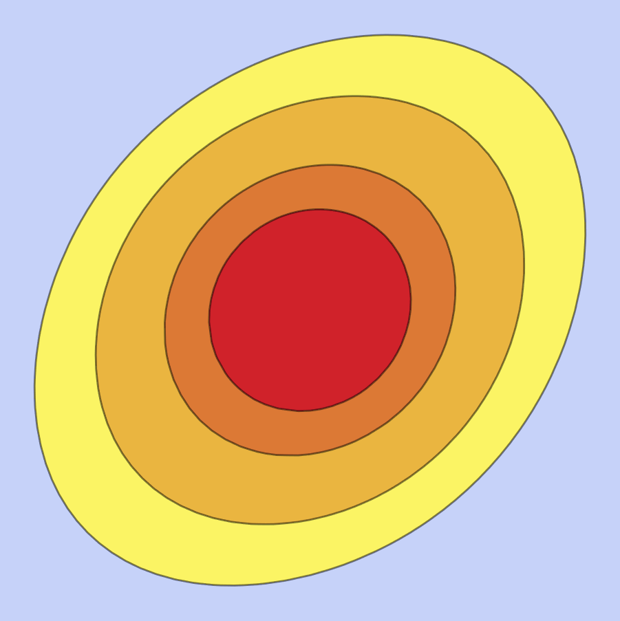
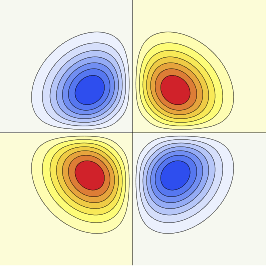
Figure 3: Level lines of the perturbation
on the square (right), and of the approximate solution on the smaller square (left).
2.3.3 Fourth order vorticity profile
We start from the following observation.
Lemma 2.8.
One has .
Proof.
Since , it follows from the definition
(2.8) that where
is a homogeneous polynomial of degree in the variable
. In particular
we have . In addition, since is radially symmetric,
we have for any :
where in the last equality we used the divergence theorem and the fact that
. This shows that has zero
radial average, hence zero projection onto the subspace .
Next we recall that , see Remark 2.7. According to
(A.6), the associated velocity field takes the form
By a direct calculation, we deduce that
Similarly, using the expression of in Lemma 2.3, we obtain
Finally, the expression above of shows that . This concludes the proof.
∎
According to Lemmas 2.8 and A.1, there
exists a unique profile
such that
(2.30)
We that choice, we obviously have
(2.31)
The results obtained in this section can be summarized as follows.
Proposition 2.9.
There exist and such that, if the profiles
of the approximate solution
(2.5) are given by (2.24), (2.27),
(2.30), then the remainder defined by
(2.21) satisfies the estimate
(2.32)
Proof.
This is a straightforward consequence of the calculations above and of the
choice of the function space . We consider the expression
(2.22) of the remainder . Using Lemma 2.2
and the fact that , we see that the last term
satisfies an estimate of the form
(2.32). This is also the case for the terms
for , because and .
Finally, in view of (2.26), (2.29), (2.31),
we have
in the topology of , which again implies an inequality of the
form (2.32).
∎
Remark 2.10.
Since , , and
, the approximate solution (2.5)
satisfies for all positive times
(2.33)
3 The solution starting from a point vortex
In this section we complete the proof of Theorem 1.6. We assume
throughout that the kinematic viscosity is small compared to the
circulation parameter , which is fixed once and for all. Given any
, we consider the unique solution of the vorticity
equation (1.2), (1.3) satisfying the conditions (1.4),
which imply that the initial vorticity is a Dirac mass of strength located
at point . Since (1.2) is a viscous conservation law, we know
in particular that for all positive times.
To desingularize the solution in the regime where is small, we make the
change of variables (2.1), where denotes the unique solution of
the modified ODE (1.14) such that . The rescaled vorticity
and the associated velocity then satisfy
the evolution equation (2.6) with initial data (1.6).
To obtain precise estimates on and , we use the decomposition
(3.1)
for all and all , where is the
approximate solution (2.5) and is the associated velocity
field. By construction, the correction terms in (3.1)
vanish at initial time , and our goal is to show that they remain small in
an appropriate topology for all . In view of (2.6),
the vorticity satisfies the evolution equation
(3.2)
for , where and is the remainder
term (2.21). The velocity is obtained from
by the usual Biot-Savart formula. Since , it follows
from Remark 2.10 that
(3.3)
The main difficulty in our analysis is the necessity of controlling the solution
of (3.2) uniformly in the small parameter . Since we
consider zero initial data, the evolution is entirely driven by the source term
in the right-hand side, which is of size according to Proposition 2.9. Note
that the fifth power of in estimate (2.32) is due to
our choice of constructing the approximate solution (2.5) as
a fourth order expansion in . Now, it follows from the
definitions (2.2) that , which
means that as long as is comparable
with .
To prove that the solution of (3.2) remains of size
over the whole time interval , we have to show that the contributions of
the source term do not get excessively amplified by the linear terms in
(3.2), which are multiplied by the large factor . This
can be done using an appropriate energy estimate in a weighted space,
where the weight function is carefully chosen so as to minimize the
contributions of the dangerous linear terms in (3.2). Note that the
nonlinear term is not multipled by , because we
chose to include a factor of in the definition (3.1) of the
corrections terms .
3.1 The short time estimate
If the observation time is small compared to the time scale defined by
(1.1), the solution of (3.2) can be controlled using a simple
energy estimate in the space defined by (2.11). To show this,
we introduce the functionals
(3.4)
where , and we observe that . We have the
following result:
Proposition 3.1.
There exist positive constants such that, if
and , the solution of (3.2) with zero initial data satisfies
(3.5)
In particular
(3.6)
Proof.
Using the definition (2.14) of the operator , we can write
the evolution equation (3.2) in the more compact form
where is the (time-dependent) linear operator defined by
(3.7)
and is the bilinear map
(3.8)
Since , it follows that
(3.9)
where denotes the scalar product in the Hilbert
space . Here we used the well known fact that
since is skew-symmetric in , see Proposition 2.5.
Our task is to estimate the various terms in (3.9).
First of all, we know that the diffusion operator is negative in the subspace of
all with zero integral, see Proposition 2.5. In fact, there
exists a constant such that
(3.10)
see [5, Lemma 5.1]. On the other hand, using Proposition 2.9, we
easily obtain
(3.11)
Note that , which also implies that since we assumed that . To bound the trilinear term in (3.9),
we integrate by parts, using the incompressibility condition , to obtain
the convenient expression
where we used the fact that . Since satisfies (3.3),
we can apply Lemma A.4 with and to obtain the bound
. By Hölder’s inequality, we thus find
where in the last step we applied the interpolation estimate to the function . Observing that and using the notation (3.4), we conclude that
(3.12)
where the last inequality follows from the fact that .
We now consider the quadratic term in (3.9)
which is multiplied by the large factor . Integrating by parts as before
we easily find
because by Lemma A.4 and . Finally, we recall that
so that
where is defined by (1.9). Assuming that is small enough so that
, we thus obtain
Altogether, since , we have shown that
(3.13)
Collecting all estimates (3.10)–(3.13), we deduce from (3.9) that
(3.14)
for some positive constants and . Since , it follows that
(3.15)
Taking small enough, we can ensure that
for all . We now define
(3.16)
with the convention that if the set above is empty. Since ,
it is clear that by continuity. By construction, on the time interval ,
the differential inequality (3.15) reduces to (3.5). In particular,
we have
where we recall that . Since we deduce that,
for all ,
(3.17)
As , the right-hand side of (3.15) is no larger
than if is small enough. We assume finally that .
Then for all , and in view of
the definition (3.16) this implies that . Thus inequalities
(3.15), (3.17) hold for all , and imply (3.5),
(3.6). This concludes the proof.
∎
3.2 Construction of the energy functional
The approach of the previous section is relatively simple and provides a control
of the solution of (3.2) in the natural function space .
However, as can be seen from the left-hand side of (3.14), the argument
completely breaks down when . To reach longer times, it is necessary
to use a more sophisticated energy functional which allows us to treat separately
three regions of the physical space: a small neighborhood of the vortex center,
an intermediate region, and a far field region where the influence of the
vortex is negligible. This idea is implemented in the previous work [4],
which deals with the interaction of localized vortices. In this section,
we provide a simplified version of the argument, which gives slightly stronger
results.
Given a small parameter , we consider the non-radially symmetric
function
Next, given positive numbers with we define the time-dependent regions
(3.20)
which are pairwise distinct and satisfy for any . Finally, we introduce the weight function
defined by the formula
(3.21)
where .
It is not difficult to verify that, if is small enough and , the inner region defined by (3.20) is
a small deformation of the disk of radius centered at the origin:
Lemma 3.2.
If is sufficiently small and for some ,
then for all the inner region is given by
(3.22)
where is smooth, -periodic, and satisfies
(3.23)
Proof.
Fix , , and assume that .
If we denote , we observe that where
(3.24)
The function is increasing on with for all
. Moreover, we know from (1.1) that and
. Assuming that , we thus find
(3.25)
provided and are small enough. This implies that the function
is strictly increasing on the interval with and
. By the intermediate value theorem, the
equation has a unique solution in
that interval, and the implicit function theorem ensures that is a smooth
function of and . Moreover, we easily deduce from (3.25) that
. If we assume that
for some , this implies that , hence . Returning to (3.24), we deduce that
(3.26)
Now, in view of the definition (3.20), we have if and only
if , which gives the formula (3.22) where
is defined by the relation
(3.27)
The expansion (3.23) follows directly from (3.26), (3.27).
∎
According to the definition (3.21), the weight function
is equal to in the (elliptical) inner region ,
at the boundary of which it takes the value by
construction. It is then extended as a constant function in the intermediate
(annular) region , and as a Gaussian function in the exterior region
. Since , we observe that when , which implies that
is a Lipschitz continuous function of . We also have
uniform bounds of the form
(3.28)
where and as .
In analogy with (3.4), we introduce the functionals that will be used
to control the solution of (3.2). The first one is the weighted energy
(3.29)
which depends explicitly on time because the coefficients
in the definition (3.18) are time-dependent. Our second functional
is
(3.30)
where
(3.31)
We can now state the main result of this section, which provides an accurate
estimate of the solution of (3.2) on the whole time interval .
Unlike in Proposition 3.1, there is no smallness assumption
on the ratio , but the various constants in the statement depend on
and on the quantity defined in (1.9).
Proposition 3.3.
If is small enough and is large enough, there exist positive constants
, , and such that, if ,
the solution of (3.2) with zero initial data satisfies
(3.32)
where , ,
and . In particular
(3.33)
3.3 The large time estimate
The goal of this section is to prove Proposition 3.3.
If is the solution of (3.2) with zero initial
data, a direct calculation shows that the energy function (3.29)
satisfies, as in (3.9),
(3.34)
for all , where the diffusion terms , the
advection terms , the nonlinear term
, and the source term are defined by
(3.35)
In (3.34) it is understood that as usual,
so that . Except for that relation, we can
consider the quantities introduced in (3.35) as defined for any fixed
and for an arbitrary value of the (small) parameter .
Useful estimates on these quantities are derived in the following paragraphs.
3.3.1 Control of the diffusion terms
Using the definition (2.4) of the differential operator and integrating
by parts, we see that
(3.36)
where
(3.37)
The quadratic form is everywhere coercive except in the region
where the weight function is independent of . The following lower
bound can be established as in [6, Prop. 4.15]. For the reader’s convenience, we
provide the details in Section A.4.
Lemma 3.4.
Assume that is small enough and . There exists a positive
constant such that, if , the following estimate holds
(3.38)
where is given by (3.31) and the regions ,
, are defined in (3.20).
Corollary 3.5.
Under the assumptions of Lemma 3.4, the diffusion term defined
in (3.35) satisfies
(3.39)
Proof.
In view of (3.36) and (3.38), what remains is to estimate
the time derivative of the weight function . In the region
we have where is given by (3.18).
Recalling that , we find
(3.40)
Using the definitions of in Lemma 2.3 and the ODE (1.14)
for , it is straightforward to verify that
(3.41)
where the constant only depends on the quantity defined in (1.9).
Since and in region ,
we deduce from (3.40), (3.41) that
where the constant depends only on and .
On the other hand, it is clear that in region , and in region
. Summarizing, we have shown that
(3.42)
Now, combining (3.36), (3.38) and (3.42), we obtain
As is easily verified, we have in region ,
so that the quantity inside square brackets is larger than
if is small enough. Similarly in region
, which implies that
if . So, assuming that , we find
where , is given by (2.9),
, and .
To estimate the quantity , we first assume that
, so that . Using the explicit
expression (3.18), we find by a direct calculation
where the last equality follows from (2.9). We thus have a partial
cancellation between the terms and , which is the reason for which we included a
non-radially symmetric correction in the definition (3.18)
of the function . It follows that
Since and for , we easily obtain
(3.44)
because in region and .
Obviously, we do not need to consider the case where ,
because in that region. When ,
we have , so that . Observing
that where is defined in (1.9),
we conclude that
(3.45)
because in region .
Combining (3.44) and (3.45), we have shown that
Multiplying by and integrating over , we obtain (3.43).
∎
We next consider the nonlocal term
Lemma 3.7.
There exists a positive constant such that .
Proof.
We deduce from (2.5) that , where is given by (1.6) and the correction
satisfies for some ,
because belongs to the function space defined in (2.13).
We can thus decompose
where
The second term is easily estimated using Hölder’s inequality:
because , see
Lemma A.3, and is uniformly
bounded. Here and in what follows, we use the uniform bounds (3.28)
satisfied by the weight function . Next, denoting ,
we observe that
by the same arguments as before. When we use the crude bound
together with the estimates (3.28)
to obtain
for some . We deduce that , which concludes the proof.
∎
3.3.3 End of the proof of Proposition 3.3 and
Theorem 1.6
In the previous paragraphs we obtained accurate bounds on the diffusion terms
and the advection term in (3.35).
As for the nonlinear term and the source term ,
they can be estimated exactly as in the proof of Proposition 3.1.
We thus find
(3.46)
for some positive constants depending on and .
It is now a straightforward task to complete the proof of Proposition 3.3.
If is the solution of (3.2) with zero initial data, we consider
the weighted energy , which evolves according
to (3.34). It is understood here that , so that
. Using the bounds (3.46) and the estimates collected
in Corollary 3.5, Lemma 3.6 and Lemma 3.7, we obtain the
differential inequality
(3.47)
where . We next choose small enough
and large enough so that
Under this assumption, inequality (3.47) implies (3.32) with
, , and replaced by .
To deduce (3.33) from (3.32), we proceed as in the
proof of Proposition 3.1. Since , we know that
at least for short times. As long as that
inequality holds, we deduce from (3.32) that
and that differential inequality can be integrated using Grönwall’s lemma
to give the estimate in (3.33). As , the conclusion remains true for all provided
is chosen small enough so that
We consider the solution of (1.2), (1.3) satisfying
(1.4), and we make the change of variables (2.1) where
is the solution of the ODE (1.14) with initial condition
. Comparing the definition (1.10) with the
expression of given in Remark 2.7, we see that
where is defined in (2.5). Using (3.1),
(3.28) and Proposition 3.3, we find
(3.48)
On the other hand, we have ,
as can be seen from the expansion (2.5) and the definition of
in Section 2.3. We deduce that ,
and together with (3.48) this concludes the proof of estimate (1.13).
∎
3.3.4 Alternative definitions of the vortex position
The results stated in the introduction are sensitive to the precise
definition of the vortex position, because they concern sharply
concentrated solutions. As is mentioned in Remark 1.7,
it is natural to consider the center of vorticity defined
by (1.15), which however does not satisfy an ODE
such as (1.8) or (1.14). Under the assumptions
of Theorem 1.6, it turns out that stays very close
to the solution of (1.14) with . To see
this, we observe that
where is defined in (2.1). Using the decomposition
(3.1) and the moment identities (2.33), (3.3),
we deduce
The right-hand side can be estimated using Proposition 3.3,
which gives
As is easily verified, this implies that estimate (1.13) in
Theorem 1.6 remains valid if the vortex position is replaced by the
center of vorticity .
On the other hand, the approximate vortex solution given by
the simple ODE (1.8) is only close to
the solution of (1.14), unless of course the additional
term in (1.14) vanishes identically. As was already
mentioned, this is the case if the external velocity field is
irrotational, see the discussion in Remark 1.1. In general, taking the
difference of (1.8) and (1.14), we obtain the inequality
which can be integrated using Grönwall’s lemma to give
(3.49)
With estimate (3.49) at hand, it is not difficult to verify that
(1.13) implies (1.7), so that Proposition 1.2
follows from Theorem 1.6. Indeed, using the bound (1.12) with
and the fact that and under
the assumptions of Theorem 1.6, we deduce from (1.13) that
(3.50)
for some constant . This estimate is similar to (1.7), except that the
Lamb-Oseen vortex is centered at the modified position , which differs
from . To obtain (1.7) from (3.50), we use the
elementary bound
together with the estimate (3.49) for the difference .
3.3.5 Alternative choice of the weight function
There is a certain amount of freedom in the choice of the weight function that is
used to control the solution of (3.2) for large times. In particular,
the diameter of the inner region should tend to infinity as
, but does not need to be proportional to , as in
(3.20). Arguably the definition (3.21) gives the
largest possible weight for which our energy estimates apply.
Compared with the previous works [4, 6, 3], where a similar approach
is implemented, our argument here provides a stronger control of the solution of
(1.2). One can also observe that the diameters of the regions
and defined by (3.20) are in the
self-similar variable , hence in the original variable , which is
quite remarkable. A minor drawback of the definition (3.21) is that
the weight is not a small perturbation of , even in the inner
region . In particular, as indicated in (3.28),
it satisfies an upper bound of the form
for , but not for .
Another interesting possibility is to use the alternative weight
(3.51)
where and the new regions ,
are defined by
Up to inessential details, this is the choice made in [4] in a related context.
The main difference with the previous definition is that the inner region is
now smaller, with a diameter proportional to instead of .
Since the outer region is unchanged, the intermediate region is proportionally larger.
The new weight satisfies uniform estimates of the form
(3.52)
for some constant . As is easily verified, the analogue of
Proposition 3.3 holds for the functionals (3.29),
(3.30) defined with the new weight , provided the
function introduced in (3.31) is replaced by
(3.53)
The estimates are even simpler because the intermediate region, where the
dangerous advection terms give no contribution, is now larger. Although
somewhat weaker, the result is still sufficient to imply Theorem 1.6.
4 The solution starting from a Gaussian vortex
In this section we prove our second main result, Theorem 1.8, by combining
the energy estimates developed in Section 3 with the enhanced dissipation
estimates established by Li, Wei, and Zhang in [13]. Let
denote the solution of (1.2), (1.3) with initial data
(1.16) at time . We make the change of variables
(2.1) for , where is the solution of the ODE (1.14)
with initial condition . The new functions and
still satisfy the evolution equation (2.6). To eliminate
the slightly unusual time derivative , it is convenient here to introduce
the new dimensionless variable
(4.1)
which is nonnegative and vanishes precisely at initial time .
the only difference being that the perturbations are now considered as functions
of the dimensionless time , instead of the original time .
As in (3.2), they satisfy the evolution equation
(4.3)
where is defined in (2.21). Here and in what follows,
it is understood that all quantities that depend explicitly on time, such
as the vortex position or the aspect ratio ,
should be considered as functions of the dimensionless variable (4.1)
via the relation .
At initial time , we have by construction
(4.4)
Using the notations of Section 2.2, we observe that , and that is of size
where . Since ,
this means that the initial data (4.4) are not small in the limit
where , which is in contrast with the situation considered in
the proof of Theorem 1.6. However, as we shall see, it is possible to decompose
the perturbation into a linear component that is initially
of size but decays rapidly as time evolves, and a correction term
which vanishes initially and remains small for all times.
4.1 Enhanced dissipation estimates
Given and , we define as the unique solution of
the linear equation
(4.5)
The spectral and pseudospectral properties of the linear operator
have been thoroughly studied in previous works, including [8, 17, 2, 5, 13].
Combining the optimal resolvent estimates obtained by Li, Wei, Zhang [13]
with the quantitative Gearhart-Prüss theorem due to Wei [27], we
immediately obtain the following result.
Proposition 4.1.
There exist positive constants and such that, for all
and all , the solution of (4.5)
satisfies
(4.6)
In particular, denoting , we have
(4.7)
Remark 4.2.
Unfortunately, it is impossible to obtain an estimate of the form (4.7)
for the gradient norm . Indeed, since the operator
is skew-symmetric in , an easy calculation shows that
where the last equality is obtained after integrating by parts. It follows that
Taking the limit and using (4.6), we see that
,
a lower bound that holds uniformly for all .
Our main result regarding the linear equation (4.5) is the following
integrated estimate for the weighted norm .
Proposition 4.3.
For any , there exists a constant such that,
for all and all
satisfying
Since , we first observe that for
some constant depending on . Next, we give ourselves a cut-off parameter
satisfying , for some (large) integer that will
be chosen later, depending only on . In view of (4.7), we have
(4.9)
which gives the first half of the desired bound. To complete the proof of (4.8),
we need an integral estimate of the quantity . This can be obtained using appropriate energy estimates, as we now explain.
First of all, we introduce the function , where
. It is easy to verify that , where
As asserted in Proposition 2.5, the operator is self-adjoint in
the space , whereas is skew-adjoint. Moreover, we have
by definition. We are interested in estimating the
norm of the function outside the disk of radius
centered at the origin. The desired localization is obtained by setting
, where and
is a smooth function satisfying
A direct calculation leads to the evolution equation , where
and with
(4.10)
The idea is now to perform a standard energy estimate in , namely
In particular, since and , we have
(4.11)
where . It remains to estimate the various terms in the
right-hand side of (4.11). We already know from (4.7) that
To bound the other terms, the following elementary observation will be useful.
Since when and
otherwise, we have for any :
(4.12)
provided with .
As a first application of (4.12), we consider the initial data . Taking such that , we can bound
and using (4.12) we deduce that .
Similarly, if , we have
Applying (4.10) and Hölder’s inequality, we thus obtain
Observing that , we see that estimate (4.8)
is a direct consequence of (4.9), (4.13).
∎
It is unclear if enhanced dissipation estimates of the form (4.6)
hold in weighted norms for . The following bound is certainly
not optimal, but will be sufficient for our purposes.
Lemma 4.4.
Assume that satisfies for some . Then there exists a constant
such that, for any , the solution of (4.5) satisfies
(4.14)
Proof.
We recall that the linear operator is the generator of a
strongly continuous semigroup in which satisfies, for any and
any , the following estimates
(4.15)
where , see [5, Section 5.1]. To prove (4.14)
we start from the integral formulation of equation (4.5), namely
We now come back to the evolution equation (4.3) for the
vorticity perturbation . We introduce the following decomposition
(4.17)
where is the solution of the linear equation (4.5). The correction
satisfies
(4.18)
where is the linear operator (3.7) and the bilinear map
(3.8). Since , the correction
vanishes at initial time, and our goal is to show that this quantity remains
small in an appropriate function space for all . As in
Section 3, the proof is much simpler if we assume that the observation
time is small compared to . So, for the sake of clarity, we first
provide the details of the argument in the simpler situation, and we return to
the general case at the end of this section.
4.2.1 Relaxation for small time
Under the assumption that , the solution of (4.18) with zero
initial data can be controlled using a simple energy estimate in the function
space , as in Section 3.1.
Proposition 4.5.
There exists a constant such that, if and , the solution of (4.18) with zero initial data
satisfies
(4.19)
for all .
Proof.
Following (3.4) we introduce the energy functional which satisfies
(4.20)
We first recall the estimates already obtained in Section 3.1. According to
(3.10), there exists a constant such that
, where
is defined in (3.4). In view of (3.12), (3.13), there
exists such that
(4.21)
Finally, the contribution of the source term can be bounded as in (3.11):
What remains is to estimate all the terms in (4.20) that involve
the solution of the linear equation (4.5). We start with the
advection term . Integrating by parts, we obtain
where . We know that ,
that for any , and
that . This gives
On the other hand we have
where . Since
we conclude that
(4.22)
We next consider the various terms involving in the quadratic form
. Integrating by parts as above, we
observe that, for all ,
We first take and , in which case
.
To estimate the norm of , we invoke [5, Lemma 5.5]
which asserts that
where in the last inequality we used the a priori estimate on
given by Lemma 4.4. We arrive at
(4.23)
The second case to consider is and . Here we
invoke [5, Lemma 5.6] which directly gives
and we conclude that
(4.24)
Summarizing, if we collect all estimates (4.21)–(4.24) we obtain
the inequality
for some positive constants and . As in Section 3.1, we suppose
that , and we work under the assumption that
, which will be verified a posteriori.
Using Young’s inequality and the fact that ,
we obtain the simpler relation
for some constant . Similarly, using Propositions 4.1 and
4.3 with , we find
because . So,
applying Grönwall’s lemma to the differential inequality (4.25), we
obtain
(4.26)
If is sufficiently small, this ensures that the a priori estimate holds whenever . Finally, since and , we see that (4.19) follows
from (4.26).
∎
4.2.2 Relaxation for large time
In the general situation where is not small, more complicated energy
functionals are needed to control the solutions of (4.18), even in
the particular case which was considered in Sections 3.2 and
3.3. As a matter of fact, the terms involving in (4.18)
do not create any real trouble, and can be treated exactly as in the proof of
Proposition 4.5. Since the estimates given by
Propositions 4.1 and 4.3 hold in the space , it is
preferable here to use the weight function defined in
(3.51), which satisfies the upper bound in (3.52).
Also, as already explained, it is convenient to express all quantities in terms
of the logarithmic time (4.1), instead of the original time .
We thus consider the energy functionals
where is defined in (3.53). Here and in what
follows it is understood that with .
The analogue of Proposition 4.5 is:
Proposition 4.6.
There exists a constant such that, if is small enough,
the solution of (4.18) with zero initial data satisfies
(4.27)
for all .
Proof.
We only give a sketch of the argument, which simply combines the estimates already
obtained in the proofs of Propositions 3.3 and 4.5.
In analogy with (3.32) we have
(4.28)
where the additional term collects all terms contributions due to ,
namely
Integrating by parts and proceeding as in (4.22), (4.23),
(4.24), we easily find
(4.29)
Here we used the fact that , see (3.52).
Applying Young’s inequality to (4.29) and returning to (4.28),
we arrive at a differential inequality of the form
where and are exactly as in (4.25).
Estimate (4.27) is then obtained by the same argument as
in Proposition 4.5.
∎
As in the proof of Theorem 1.6 we estimate the quantity
where we used the decompositions (4.2) and (4.17).
To bound the first term in the right-hand side, we apply Proposition 4.1,
and we recall that where , see (4.4). Since ,
we find
where . For the second term we invoke
Proposition 4.6 which gives
where we used again the relation . Altogether arrive at
(4.30)
and the second integral that appears in the the proof of Theorem 1.6 satisfies
, so that .
Estimate (1.17) thus follows from (4.30).
∎
Appendix A Appendix
A.1 Comparison with the Burgers vortex
We consider here the simple example of a time-independent velocity field
of the form
(A.1)
where the strain rate is a parameter. Using the definitions
(1.1), (1.11), we see that , ,
and in the present case. Let be the solution of
(1.2), (1.3) satisfying
as . Applying the self-similar change of coordinates (2.1) with
, we obtain the evolution equation (2.3) which takes the form
(A.2)
where is defined in (2.4) and . If we freeze time in (A.2), we arrive
at the elliptic equation
(A.3)
where . This is exactly the equation satisfied by
the profile of a Burgers vortex with Reynolds number
and asymmetry parameter , see [23, 22, 9]. In particular
the results of [9, 15, 16] show that, if is
fixed and is sufficiently small, equation (A.3)
has a unique solution which satisfies
(A.4)
where is precisely the function considered in Remark 2.7.
Comparing (A.4) with approximate solution (1.10)
in the particular case of the external field (A.1), we deduce
that
This means that, for and sufficiently small,
the approximate solution (1.10) is a simple rescaling of the
vorticity profile of a Burgers vortex with asymmetry parameter and Reynolds number .
A.2 Partial inverse for the advection operator
In this section, for completeness, we recall the known formulas for the
(partial) inverse of the integro-differential operator defined in
(2.14). More details can be found in the references
[4, 6]. Since leaves invariant the direct sum decomposition
(2.12), it is sufficient to study the restriction of to each
subspace . Actually by (2.15),
so we can assume that . To exploit the rotational symmetry, we use polar
coordinates in defined by , and we
introduce the radially symmetric functions
Assume that takes the form for some
function . As is easily verified, the associated velocity field is
(A.6)
where , , and is the unique
solution of the ordinary differential equation
(A.7)
satisfying the boundary conditions as and
as . Using (A.5), (A.6),
we easily obtain
(A.8)
Similarly, if , then .
Now we give ourselves a function of the form .
If the inhomogeneous differential equation
(A.9)
has a (unique) solution satisfying the boundary conditions, we define
with
(A.10)
which is depicted in Figure 2 in the case .
Then (A.7) is obviously satisfied, and (A.8) implies
that . The same conclusion holds if and
. The level lines of in the case are depicted on
the right of Figure 3.
This discussion shows that the invertibility of the operator in
the subspace is linked to the solvability of the ODE (A.9).
The favorable case is , because the coefficient is positive,
which ensures that (A.9) has a unique solution satisfying the boundary
conditions. If is the function space (2.13), we thus obtain the
following result:
Lemma A.1.
[4]
If and , there exists a unique such that . Moreover, if
(respectively, ) then
(respectively, ) where is defined
by (A.10) with given by (A.9).
If , the homogeneous differential equation (A.9) with
has a nontrivial solution which satisfies the boundary
conditions. As a consequence, the inhomogeneous equation can be solved only if
the right-hand side satisfies , and the solution
is never unique. The solvability condition ensures that belongs to the subspace
defined by
(A.11)
see also (2.17). We have the following result, which
complements Lemma A.1.
Lemma A.2.
[6]
If and , there exists a unique such that . Moreover, if
(respectively, ) then
(respectively, ) where is defined
by (A.10) with given by (A.9).
A.3 Estimates on the velocity field
We collect here, for easy reference, a few classical estimates on the Biot-Savart
operator (1.3) which are used in the proof of our main results. Given
a vorticity distribution , we define as in (1.3).
Lemma A.3.
[7, Lemma 2.1] Assume that
.
1) If then .
2) If with ,
then .
Let be the weight function defined by for .
Lemma A.4.
[7, Proposition B.1]
Assume that .
If and , then
for all .
In particular, by Hölder’s inequality, .
Let be the function space defined by (2.13). The following
statement can be established using the same arguments as in
[7, Appendix B].
Lemma A.5.
If , then and . Moreover:
1) If , then ;
2) If and for ,
then .
The parameter does not play any role in the argument here, so we
omit the time dependence of all quantities. Given sufficiently
small, we give ourselves two smooth and radially symmetric functions
such that
for all , whenever ,
and whenever . It is well-known
that such a partition of unity exists, and we can also assume that for all .
Given we define and , so
that . A direct calculation shows that .
Thus, recalling the definition (3.37) of , we have
(A.12)
It is therefore sufficient to obtain lower bounds on the quantities
and .
To estimate we apply Hölder’s inequality to obtain
so that
(A.13)
Using the definition (3.21) of the weight , it is not
difficult to verify that, under the assumptions of Lemma 3.2,
We further observe that as soon as
, and that vanishes for , which
implies that
for some . Thus, assuming that are as in
Lemma 3.2, we obtain the lower bound
(A.14)
On the other hand, since is supported in the region where the weight
is smooth, we can define and
integrate by parts to show that , where
It is easy to verify that when , so that is close to when
is small. Note that and ,
so that is the quadratic form of the quantum harmonic oscillator with
ground state , see [7, Appendix A]. In particular,
if , it is known that .
In our case, since we assume that , the orthogonality
condition above is nearly satisfied in the sense that
where we used that for ,
and that . If is sufficiently small, we deduce that
(A.15)
Observing that inequality (A.13) also holds with replaced by ,
we add of (A.15) and of (A.13) to arrive at the
lower bound
(A.16)
for some . Finally, estimate (3.38) is a direct
consequence of (A.12), (A.14), (A.16).
Acknowledgements. The research of both authors is supported
by the grant BOURGEONS ANR-23-CE40-0014-01 of the French National Research Agency.
References
[1]
[2] Wen Deng, Pseudospectrum for Oseen vortices operators,
Int. Math Res. Notices 2013 (2013), 1935–1999.
[3]
M. Dolce and Th. Gallay,
The long way of a viscous vortex dipole, preprint arXiv:2407.13562.
[4] Th. Gallay,
Interaction of vortices in weakly viscous planar flows,
Arch. Rational Mech. Anal. 200 (2011), 445–490.
[5] Th. Gallay,
Enhanced dissipation and axisymmetrization of two-dimensional viscous vortices,
Arch. Rational Mech. Anal. 230 (2018), 939–975.
[6]
Th. Gallay and V. Šverák,
Vanishing viscosity limit for axisymmetric vortex rings, Invent. Math.
237 (2024), 275–348.
[7] Th. Gallay and C. E. Wayne,
Invariant manifolds and the long-time asymptotics of the
Navier-Stokes and vorticity equations on ,
Arch. Ration. Mech. Anal. 163 (2002), 209–258.
[8]
Th. Gallay and C.E. Wayne,
Global stability of vortex solutions of the two-dimensional
Navier-Stokes equation, Commun. Math. Phys. 255 (2005),
97–129.
[9]
Th. Gallay and C.E. Wayne,
Existence and stability of asymmetric Burgers vortices,
J. Math. Fluid Mech. 9 (2007), 243–261.
[10]
I. Gallagher and Th. Gallay,
Uniqueness for the two-dimensional Navier-Stokes equation with a measure as initial
vorticity, Math. Ann. 332 (2005), 287–327.
[11]
Y. Giga, T. Miyakawa, and H. Osada,
Two-dimensional Navier-Stokes flow with measures as initial vorticity,
Arch. Rational Mech. Anal.104 (1988), 223–250.
[12]
S. Le Dizès and A. Verga,
Viscous interactions of two co-rotating vortices before merging,
J. Fluid Mech. 467 (2002), 389–410.
[13]
Te Li, Dongyi Wei, and Zhifei Zhang,
Pseudospectral and spectral bounds for the Oseen vortices operator,
Ann. Sci. Ecole Normale Supérieure 53 (2020), 993–1035.
[14]
C.H. Liu and L. Ting, Interaction of decaying trailing vortices in spanwise shear
flow. Comput. Fluids 15 (1987), 77–92.
[15]
Y. Maekawa,
On the existence of Burgers vortices for high Reynolds numbers.
J. Math. Anal. Appl. 349 (2009), 181–200.
[16]
Y. Maekawa,
Existence of asymmetric Burgers vortices and their asymptotic behavior at large
circulations, Math. Models Methods Appl. Sci. 19 (2009), 669–705.
[17] Y. Maekawa,
Spectral properties of the linearization at the Burgers vortex
in the high rotation limit, J. Math. Fluid Mech. 13 (2011), 515–532.
[18] A. J. Majda and A. L. Bertozzi,
Vorticity and Incompressible Flow, Cambridge University Press, 2002.
[19]
C. Marchioro, On the inviscid limit for a fluid with a concentrated
vorticity, Commun. Math. Phys. 196 (1998), 53–65.
[20]
C. Marchioro and M. Pulvirenti, Mathematical theory of
incompressible nonviscous fluids, Appl. Math. Sci. 96, Springer, 1994.
[21]
P. Meunier, S. L. Dizès, and T. Leweke, Physics of vortex
merging, C. R. Phys. 6 (2005), 431–450.
[22]
H. K. Moffatt, S. Kida, and K. Ohkitani,
Stretched vortices—the sinews of turbulence; large-Reynolds-number asymptotics,
J. Fluid Mech. 259 (1994), 241–264.
[23]
A. C. Robinson and P. G. Saffman,
Stability and structure of stretched vortices,
Stud. Appl. Math. 70 (1984), 163–181.
[24]
L. Ting and R. Klein,
Viscous vortical flows, Lecture Notes in Physics 374,
Springer, 1991.
[25]
L. Ting, R. Klein, and O. Knio,
Vortex Dominated Flows. Analysis and Computation for Multiple Scale
Phenomena, Appl. Math. Sci. 161, Springer, 2007.
[26]
L. Ting and C. Tung, Motion and decay of a vortex in a nonuniform stream,
Phys. Fluids8 (1965), 1039–1051.
[27] Dongyi Wei, Diffusion and mixing in fluid flow via the resolvent
estimate, Sci. China Math. 64 (2021), 507–518.
Martin Donati
Institut Fourier, Université Grenoble Alpes, CNRS
100 rue des Maths, 38610 Gières, France
Email Martin.Donati@univ-grenoble-alpes.fr
Thierry Gallay
Institut Fourier, Université Grenoble Alpes, CNRS, Institut Universitaire de France
100 rue des Maths, 38610 Gières, France
Email Thierry.Gallay@univ-grenoble-alpes.fr