O0pt O.8 m t! e_^ #3\IfValueT#5 \IfBooleanTF#4_\scaleobj#2#5_#5 \IfValueT#6^#6 \RenewDocumentCommandßO0pt O0pt O.8 m e_^ #4\IfValueT#5 _\scaleobj#3#5 \IfValueT#6 ^\scaleobj#3#6
Tropical function fields, finite generation, and faithful tropicalization
Abstract.
Given an algebraic variety defined over a discrete valuation field and a skeleton of its Berkovich analytification, the tropicalization process transforms function field of the variety to a semifield of tropical functions on the skeleton. Our main result offers a purely polyhedral characterization of this semifield: we show that a tropical function is in the image of the tropicalization map if and only if it takes the same slope near infinity along parallel half-lines of the skeleton. This extends a result of Baker and Rabinoff in dimension one to arbitrary dimensions. We use this characterization to establish that this semifield is finitely generated over the semifield of tropical rational numbers, providing a new proof of a recent result by Ducros, Hrushovski, Loeser and Ye in the discrete valued field case. As a second application, we present a new proof of the faithful tropicalization theorem by Gubler, Rabinoff and Werner in the discrete valuation field case. The proof is constructive and provides explicit coordinate functions for the embedding of the skeleton, extending the existing results in dimension one to arbitrary dimensions.
1. Introduction
Throughout this paper, let be a complete discrete valuation field with valuation , valuation ring with maximal ideal , and residue field .
Let be a smooth projective geometrically connected variety over and let be a strictly semistable model of , defined over the valuation ring of some finite extension of . Let denote a horizontal divisor of such that forms a strictly semistable pair. The special fiber of is denoted by . After performing a possible finite base change, we assume that each connected component of the intersection of any collection of irreducible components of is geometrically connected.
Let be the dual complex of , an abstract polyhedral complex with a recession fan defined as follows. Let for be the irreducible components of and for the irreducible components of . To any connected component of an intersection of the form
where is nonempty and , we associate a copy of the polyhedron . Here, is the standard simplex in consisting of points with non-negative coordinates summing to one. The collection of these polyhedra forms , which glue together to define the polyhedral space to which we refer as the support of . Moreover, the collection of cones consisting of a copy of associated with each connected component of a nonempty intersection of the form , as above, forms an abstract fan referred to as the recession fan of . These cones glue together and form the support of . In particular, the rays of correspond to the components of . See Sections 2.2 and 3 for more details.
Two rays in are said to be parallel if they are associated with the same component of , meaning they correspond to the same ray in . More generally, two half-lines in are parallel if the corresponding half-lines issued from the origin in are the same.
Let denote the Berkovich analytification of (see [Ber90]). The dual complex (more precisely, its support) naturally embeds in forming a subspace called the skeleton of associated with . This allows to identify with .
Let denote the function field of . Identifying with the skeleton , we associate to each point a valuation
For any , the (abstract) tropicalization of is defined as
More generally, consider the base change of to an algebraic closure of . The tropicalization map naturally extends to , and for , it yields a function , as described above, on .
The set of tropicalized rational functions on is a semifield with the operation of addition corresponding to taking pointwise minimum of functions, and the operation of multiplication corresponding to the usual addition.
Our first main result gives a characterization of this semifield. This is done as follows.
We define as the union of and the space of facewise integral -affine functions on which take the same slope near infinity along parallel rays of . Similarly, we define as the union of and the space of piecewise integral -affine functions on which exhibit the same slope near infinity along parallel half-lines of . Equivalently, is the union of over integral -affine refinements of (see Section 2.2). We refer to as the tropical function field of .
Theorem 1.1 (Characterization Theorem).
For every , the tropicalization belongs to . The resulting map
| (1.1) |
is surjective.
Consequently, the tropical function field coincides with the semifield of tropicalized rational functions on .
This result generalizes the work of Baker and Rabinoff [BR15] in dimension one to arbitrary dimensions, while also accounting for the presence of horizontal divisors. See also the work of Amini and Iriarte [AI22], which addresses the case of trivially valued fields of characteristic zero, and establishes the surjectivity of an analogous tropicalization map, defined relative to a compactification. We note that our proof of the characterization theorem gives the surjectivity of tropicalization map from to for an extension of with value group .
To state our second main result, we recall that a semifield is said to be finitely generated over a semifield if there exist finitely many elements of such that every element of can be expressed as with and -variable polynomials over .
Let denote the semifield of rational numbers with the operations of min for addition and for multiplication. We observe that the definition of tropical function fields extends to any abstract polyhedral complex endowed with a recession fan (see Section 2.2).
Theorem 1.2 (Finite generation of tropical function fields).
Let be an abstract polyhedral complex with a recession fan. The tropical function field is finitely generated over .
In particular, as above is finitely generated over . In a recent work [DHLY24], using model theory of valued fields, Ducros, Hrushovski, Loeser, and Ye prove that is finitely generated as a semifield over the value group. A combination of our Theorems 1.1 and 1.2 yields a new proof of their result in the discrete valued field case, showing in addition the finite generation of for an extension of with value group without requiring to be defectless. Note that as it was stated in [DHLY24], finite generation property does not hold in general for .
As an application of Theorems 1.1 and 1.2, we provide an alternative proof of the faithful tropicalization theorem of Gubler, Rabinoff, and Werner [GRW16] in the discrete valued field case. See also [Duc12, Thm 5.1] and [DHLY24, §1.2].
Theorem 1.3 (Gubler–Rabinoff–Werner [GRW16]).
Let be a smooth projective variety over with a strictly semistable pair , as above. Then, there exist such that, setting , the map
provides a faithful tropicalization of the skeleton of , that is, the restriction of to is a homeomorphism onto its image that preserves the integral structures.
Our proofs of Theorems 1.1, 1.2 and 1.3 yield additional insights. We explicitly construct such that the map
is a homeomorphism onto its image preserving the integral structures. By Theorem 1.1, there exist satisfying . Our proof shows that the embedding given by provides a faithful tropicalization of the skeleton as stated in Theorem 1.3. Moreover, generate , which is equal to by Theorem 1.1. In particular, the proof provides explicit coordinate functions for the embedding of the skeleton. This way, we extend the existing results on effective tropicalization in dimension one [BPR16, CM19, Hel19, KMM08, KY21, MRS23], and for special varieties of higher dimension [CHW14, DP16, Kut16, KY19, Ran17], to arbitrary varieties in all dimension.
Our proof of Theorem 1.2 gives a stronger result. Let be an integral -affine polyhedral complex in . We define to be the set consisting of and piecewise integral -affine functions on which that take the same slope near infinity along any pair of parallel half-lines in (see Definition 2.2).
Let denote the subsemifield of the semifield of piecewise integral -affine functions on generated by the coordinate functions . Then, we have a natural restriction map
We denote by the kernel of as a congruence. For the notion of a congruence, which serves as the analogue of an ideal when forming a quotient in the context of semirings, see Section 3.6.
Theorem 1.4.
The restriction map is surjective, meaning that the restrictions of the coordinate functions to generate the semifield over . Moreover, is finitely generated as a congruence.
This generalizes a result of Song [Son24] in dimension one to arbitrary dimensions when is defined over .
As a final remark, although we have restricted our focus to the case of discretely valued fields in order to avoid technicalities and have a clearer presentation, we are confident that the arguments employed in this work can be extended to more general valued fields. Moreover, the condition on being smooth, projective and geometrically connected is not restrictive, since our results on tropicalizations concern birational geometry of varieties over an algebraic closure of .
The text is organized as follows. In Section 2, we provide preliminaries on polyhedral geometry, followed by background materials on tropical and non-Archimedean geometry in Section 3. Theorem 1.1 is proved in Section 4. The proofs of Theorems 1.2, 1.3, and 1.4 are given in Section 5.
Acknowledgment. This project started during the workshop “Nonarchimedean geometry and related fields” in Kyoto in January 2024. We thank the organizers of the workshop and Kyoto University for hospitality. We thank Matthieu Piquerez and Kazuhiko Yamaki for helpful discussions. O.A. is part of the ANR project AdAnAr (ANR-24-CE40-6184). S.K. is partially supported by KAKENHI 23K03041 and 20H00111.
2. Polyhedral complexes
We gather some definition and notation regarding embedded and abstract polyhedral complexes.
2.1. Polyhedral complexes in
We denote the points of with bold letters with coordinates .
Let denote the standard inner product of . An integral -affine function on is a function of the form
for some and . A function of the above form with and is called an affine function.
An integral -affine polyhedron in is a subset of the form
for integral -affine functions on . Each face of an integral -affine polyhedron is again integral -affine. When is compact, it is called an integral -affine polytope. If the s in the definition of are integral linear, then is called a rational cone.
An integral -affine polyhedral complex in is a polyhedral complex whose cells are integral -affine. Recall that this means is a finite collection of integral -affine polyhedra such that
-
•
for each , any face of is included in .
-
•
for each pair with nonempty intersection, is a common face of and .
Let be an integral -affine polyhedral complex in . For , we write if is a face of . A ray of is an unbounded one-dimensional element in . The support of denoted by is the union of polyhedra . We say that is complete if .
Each integral -affine polyhedron in can be expressed as a sum , where is an integral -affine polytope and is a rational cone, uniquely determined by . We refer to as the recession fan of , and denote it by . When the collection , for , forms a fan, we call it the recession fan of , see [BGS11].
Let be two integral -affine polyhedral complexes in . We say that is a refinement of if and for each , there exists with .
Let be an integral -affine polyhedron. An (integral -)affine function on is by definition the restriction to of an (integral -)affine function .
We define the space of facewise, resp. piecewise, (integral -)affine functions on , resp. , as follows.
Definition 2.1 (Facewise (integral -)affine functions and ).
Let be an integral -affine polyhedral complex in . We say that is facewise (integral -)affine on if is (integral -)affine for any .
We denote by the union of and the space of facewise integral -affine functions on which take the same slope at infinity along any pair of parallel rays in . Similarly, we define as the union of and the space of all facewise affine functions on which take the same slope at infinity along any pair of parallel rays in . ∎
Definition 2.2 (Piecewise (integral -)affine functions and ).
Let be an integral -affine polyhedral complex in . We say that is piecewise integral -affine if there exists an integral -affine refinement of such that the restriction is an integral -affine function on for each . We denote by the union of and the space of all piecewise integral -affine functions , as above, where takes the same slopes at infinity along any two parallel half-lines of .
Similarly, we define piecewise affine functions on and , by removing the integrality constraint. ∎
Note that each element belongs to for some integral -affine refinement of . Moreover, a pair of integral -affine refinements and have a common integral -affine refinement. Therefore, is closed under addition and taking minimum. This turns into a semifield (see Section 3.5). The same remark applies to .
For future use, we define convex functions on integral -affine polyhedral complexes.
Definition 2.3 (Convex function).
Let be an integral -affine polyhedral complex in and let be a facewise (integral -)affine function on . We say that is convex if, for any , there exists an (integral -)affine function such that and
on for each with . We say that is strictly convex if the inequalities above are strict on . ∎
We say that a function is concave if is convex.
Definition 2.4 (Convexity of a polyhedral complex).
An integral -affine polyhedral complex is said to be convex if there exists a strictly convex function . ∎
2.2. Abstract polyhedral complex with a recession fan
For a set , we denote by the power set of .
An abstract polyhedral complex with a recession fan is defined as follows. Let and be two disjoint finite sets, with nonempty. Let be a finite delta-complex on the set . This means that is a finite set endowed with a partial order and there exists a map with the following properties:
-
()
There exists a minimum element in , denoted by , with .
-
()
For each , there exists a unique element of with .
-
()
For each , the restriction of to the interval is a bijection with the poset of subsets of . Here, the partial order on subsets is given by inclusion.
In particular, for each pair of elements in , we have .
Denote by the set of all elements of with nonempty intersection with . We call an abstract polyhedral complex with vertex set and recession rays . By an abuse of the notation, we denote the restriction of to by . The complement is itself a delta-complex. Let be the abstract polyhedral complex with vertex set and recession rays which as a set is equal to endowed with the same partial order , with the map defined by for all . Although the definition of is dependent on , by an abuse of the notation we refer to as the recession fan of , and call an abstract polyhedral complex with recession fan .
Given a nonempty subset and a subset , we define the extended simplex
where denotes the non-negative orthant in , and denotes the standard simplex in ,
| (2.1) |
We denote by , , the standard basis of .
Given an abstract polyhedral complex with recession fan as defined above, we associate to each element a copy of the polyhedron . The property () ensures that the polyhedra are nonempty and they glue together, along inclusions, for each pair of elements in , of as a face of .
The resulting space is denoted by and is called the support of . When there is no risk of confusion, we simplify the notation and write in place of .
Using this simplified notation:
-
•
The finite part of is denoted by and corresponds to the simplex .
-
•
The infinite part of is denoted by , it corresponds to the cone and naturally belongs to .
Similarly, we define , the support of the recession fan , by gluing the collection of , identified with , for all . (This can be viewed as a multifan in .)
A ray in is an element with and each have size one. Two rays and are parallel if they correspond to the same element of .
More generally, two half-lines in are parallel if they correspond to the same half-line issued from the origin in .
Example 2.5.
-
(1)
Let and . We set
and set
Then, a half-line in is parallel to a half-line in if they are either parallel to or they are parallel to .
-
(2)
We take the same example as above, but we change to
In this second example, the recession cones of and are the same, and so a half-line in is parallel to a half-line in if they are the same half-line in . ∎
An integral -affine refinement of consists in a collection of integral -affine refinements of each , in the sense of the previous section when is viewed as embedded in . These refinements are required to be compatible with each other along inclusion of faces. Two rays in are parallel if they are parallel half-lines in .
Given an abstract polyhedral complex with recession fan , we define as the union of and the space of facewise integral -affine functions on which take the same slope near infinity along parallel rays of . We define as the union of and the collection of all facewise integral -affine functions on some integral -affine refinement which take the same slopes near infinity along parallel rays of . Equivalently, is the union of and the collection of all piecewise integral -affine functions on which take the same slope near infinity along two parallel half-lines in . The set has the structure of a semifield with addition corresponding to taking pointwise minimum of functions, and multiplication corresponding to the usual addition (see Section 3.5).
3. Tropical preliminaries
The purpose of this section is primarily to provide definitions and establish notation. For further details, we refer the reader to [Ber90, Ber99, Ber04, GRW16, BFJ16, dJ96, KY19, MN15].
3.1. Notation and conventions
As in the introduction, let be a complete discrete valuation field. Let be the valuation ring of , the maximal ideal of , and the residue field. We fix a uniformizer of . Let be the valuation map with .
By a variety over we mean an irreducible, reduced, and separated scheme of finite type over . By a variety over , we mean an irreducible, reduced, and separated scheme , flat and of finite type over . The special fiber of is denoted by , and the generic fiber of is denoted by .
3.2. Semistable models and skeleta
Let be a projective variety over of dimension . Let , , denote the irreducible components of the special fiber . For a subset , we put . We say that is strictly semistable if is covered by open subsets that admit an étale morphism
Under these conditions, is regular, the special fiber is reduced, and for each subset , each connected component of is smooth over . For further details, see [GRW16, Definition 3,1] and [dJ96, 2.16].
Let be a smooth projective variety of dimension over . A strictly semistable model of over is a strictly semistable projective variety over endowed with an isomorphism over .
Let be a projective variety over of dimension . Let be a sum of finitely many hypersurfaces on , where the are irreducible and pairwise distinct. We set .
We say that the pair is a strictly semistable pair if is covered by open subsets which admit an étale morphism
for such that the restriction of to is either trivial or defined by for some . In this case, is strictly semistable, is a divisor with strict normal crossings on , and for each , is a disjoint union of varieties over , which are themselves strictly semistable over , cf. [GRW16, Definition 3,1] and [dJ96, 6.3, 6.4]. We refer to the , , as the horizontal components and to the , , as the vertical components of .
Given a smooth projective variety defined over , we say that is a strictly semistable pair of if is a strictly semistable model of .
From a strictly semistable pair of , we obtain a delta-complex giving rise to an abstract polyhedral complex and a recession fan , and the corresponding skeleton in , with its integral polyhedral complex structure, as follows.
Stratification
Let be a strictly semistable pair of . By the definition of a strictly semistable pair, is a reduced divisor on , and each irreducible component of is either a connected smooth projective variety over (for the , ), or a connected regular projective variety over (for the , ).
We define a stratification of as follows. We put , and for each , we let be the complement of the set of regular points in . Thus, we obtain a chain of closed subsets:
where .
We say that is a stratum of if there exist subsets and such that is a nonempty connected component of . We say that is special if . Note that is a special stratum if and only if and .
Dual complex and (extended) simplices associated with special strata
Let be the set consisting of an element and other elements in bijection with the strata of . We endow this set with the partial order corresponding to the reverse inclusion of strata, and declaring that is the minimum element. We define the map , by setting and sending each stratum to the union of the corresponding index sets and . This turns into a delta-complex on the set .
Let be the corresponding abstract polyhedral complex and the corresponding recession fan in the sense of Section 2.2. Specifically, is the set of elements in bijection with the special strata of . We refer to as the dual complex of .
Let , , be a special stratum of with the corresponding index sets and as above. We associate to the extended simplex .
There is a canonical embedding of in , defined as follows. To each , we associate an absolute value on the function field which extends . Let be the generic point of . For each and , we choose a local equation of and of in at .
Let be the completion of . By [MN15, §2.4], each element has an expansion of the form
where each coefficient is either zero or a unit in . Such an expansion is called an admissible expansion of .
We write , and set
| (3.1) |
By [MN15, Proposition 2.4.4], is a well-defined absolute value on . This absolute value extends to an absolute value on . Furthermore, since for some unit in , we have , which shows that agrees with for elements in . Thus, for each , we have a point lying on the generic point of .
With the above notation, the assignment
| (3.2) |
is a homeomorphism, cf. [MN15, Proposition 3.4], [GRW16, 4.2, 4.3]. We thus get an identification
| (3.3) |
The polyhedron is endowed with a natural integral affine structure.
Note that by the construction, is independent of the choice of local equations and for and . Thus, the embedding of in the Berkovich space given in (3.2) is intrinsic, cf. [GRW16, p. 169].
Let be another special stratum such that the Zariski closure of contains . Then, is a face of . Moreover, the embedding of and in are compatible, as we now explain. Since and is a special stratum, there exist a subset of and a subset of such that is defined in at its generic point by for all and for all . The extended simplex is the face of consisting of those points with for and for .
Then, by the very definition of , we see that for any . It follows that the embedding of in coincides with the restriction to the face of the embedding of in .
Skeleton
The skeleton associated with the strictly semistable pair is defined by
The skeleton can be identified with the support of , embedded in .
In the following, we often denote by the elements of . For two elements in , we write
| (3.4) |
if is a face of , equivalently, if .
Parallel rays in and parallel half-lines in
We define parallel rays of as in Section 2.2. Identifying with the support of , we define the notion of parallel half-lines for the skeleton.
3.3. Tropicalization and the tropical function field of
We retain the notation and assumptions introduced in the previous subsection.
We define and as in Section 2.2. The latter, , is referred to as the tropical function field of .
Let be a nonzero element. Let , and let and such that , see (3.3). We set
This yields a function
We extend the definition by setting .
Proposition 3.1.
For each , we have .
Proof.
We may assume that . Take a special stratum , . Let and be the subsets such that is a connected component of . We write with , where is the generic point of .
Using the notation from (3.1), we represent and by admissible expansions
For each , we have
It follows that is a continuous piecewise integral -affine function.
Furthermore, let be a ray in parallel to . Let be the horizontal irreducible component of corresponding to . The slope of near infinity along equals to the order of vanishing of along , which remains constant for rays parallel to .
More generally, on each , is the difference of the two functions , where each is the tropicalization of . Since is the minimum of affine functions consisting of a bounded term () and an unbounded term (), and similarly for , the asymptotic behavior near infinity of is captured by the minimum of their unbounded term
Let be the stratum of which contains and is a connected component of the intersection . Denote by the generic point of . The admissible expansion for at given above provides an admissible expansion of at of the form
where and . The associated cone of lives in the Berkovich analytification of , when is viewed as a trivially valued field. The tropicalization of on is given by the admissible expansions in the form and , and does not depend on the choice of admissible expansions (see [JM12, Proposition 3.1]). This is equal to .
By the definition of parallel half-lines in , we infer that has the same slope near infinity along two parallel half-lines in .
We infer that belongs to . ∎
Let be an algebraic closure of . Let . Recall that we assume that and each connected component of the intersection of any collection of irreducible components of are geometrically connected.
Proposition 3.2.
The tropicalization map extends to .
Proof.
Let be a finite field extension of , and let , where . Denote by the integral closure of in . Then, is a discrete valuation ring (see [Mat80, Chap. 12, Th. 72]). Let be a uniformizer of , and recall that denotes a uniformizer of . We can write
The base change is expressed étale locally as
By Theorem 4.1, there exists a regular strictly semistable model along with a surjective morphism . Let be the natural morphism and set . Let be the strict transform of by . Then, is a strictly semistable pair on , and forms an integral -affine refinement of . In particular, the skeleton is naturally identified with . By our assumption, the recession fan of is the same as that of .
By applying Proposition 3.1 to , we obtain the tropicalization map
For , viewed in , the tropicalization obtained above coincides with the previously defined tropicalization.
Hence, we obtain the tropicalization map . ∎
3.4. Faithful tropicalization
We recall the definition of faithful tropicalization; see [GRW16, §9] for further details.
Let be a strictly semistable pair, where is a strictly semistable model of defined over .
Given nonzero rational functions , let be the open subset of obtained by removing the support of the divisors , . Consider the map from to the algebraic torus . The tropicalization of induces a map .
Since the skeleton is included in , the restriction of gives a map
We say that is faithful if the following conditions are satisfied:
-
•
The restriction of to the skeleton is injective.
-
•
On each , , the restriction is piecewise integral -affine.
-
•
The inverse of from to is also piecewise integral -affine.
Equivalently, is faithful if it is injective, its image is an integral -affine polyhedral complex in , and the inverse map from the image of to is piecewise integral -affine.
3.5. Semifields and finite generation
We set
For , we set
With these operations, forms a semifield, where is the identity element for and is the identity element for . We call the tropical semifield.
Similarly, we define the tropical subsemifield as
Let be a semiring with binary operations and . We say that is a semiring over if there exists an injective semiring homomorphism . In this case, for any and , the operation is well-defined via this homomorphism. Moreover, if is a semifield, we call it a semifield over .
Example 3.3 ().
Let be defined as in Definition 2.2. For and , we define
Under these operations, , , and all belong to . Moreover, forms a semiring over . Furthermore, for any other than , we have . This shows that is a semifield over . ∎
Let be a semiring over , and . Define the subsemiring of generated by as
The semifield of fractions of denoted is defined by localizing at its nonzero elements. If is a semifield, then .
Definition 3.4 (Finitely generated semifields).
Let be a semifield over . We say that is finitely generated as a semifield over if there exist such that . ∎
3.6. Congruences
Let be a semiring with binary operations for addition and for multiplication. An equivalence relation on is a congruence if it satisfies the following property: For any , if and , then
We refer to [HW93, §I.7] for further details.
If is a congruence on , then the quotient is itself a semiring. Conversely, if is a semiring homomorphism, then the kernel
is a congruence on . In the context of semirings, the operation of taking the quotient of a ring by an ideal is replaced by taking the quotient by a congruence.
Definition 3.5 (Finite generation property for congruences).
Let be a congruence on . We say that is finitely generated if there exist elements with for all such that the following holds:
If denotes the minimal congruence on generated by the relations , then coincides with . ∎
4. Characterization theorem
As before, let be a complete discrete valuation field. Given a finite extension of , we denote by the integral closure of in , and by the residue field of .
Let be a smooth, geometrically connected, projective variety over , and suppose that admits a strictly semistable model over . Let be a strictly semistable pair, and assume that each connected component of the intersection of any collection of irreducible components of is geometrically connected. Let be the dual complex of , and let be the associated skeleton. Denote by the recession fan of .
In this section, we prove Theorem 1.1. Specifically, we show that for any in the tropical function field , there exists an element such that .
Theorem 4.1.
Notation as above:
-
(C1)
There exist a finite extension field , a strictly semistable model of and a morphism with the following properties:
-
(i)
Let be the strict transform of by . Then, is a strictly semistable pair, and is a subdivision of with the same recession fan.
-
(ii)
Let , , be the irreducible components of , and , be the irreducible components of . Then, for any subset and , the intersection is either empty or irreducible.
-
(i)
-
(C2)
Let . Then, there exists a finite extension field and a strictly semistable model of satisfying Properties (i) and (ii) of (C1) such that .
Proof.
We follow the desingularization procedure described in [Har01], which involves performing successive below-ups, adapted to the strata obtained from intersections of the components of and those of the special fiber. This process results in a semistable model with a map . The corresponding dual complex yields a triangulation of the dual complex of . More precisely, it forms an order subdivision of , in the sense of [Car21], where is the ramification index of . For , this subdivision has no multiple faces. Moreover, by our assumption on , the recession fan does not change, from which (C1) follows.
For each , there exists a large and an -subdivision of as above over which is facewise integral -affine. The second statement follows. ∎
Our strategy for proving Theorem 1.1 goes as follows. By replacing with and with , we may and do assume that our model satisfies the properties stated in (C1) and (C2) of Theorem 4.1, and that is facewise integral -affine on each (extended simplex) associated with a special stratum of . Moreover, passing to a large field extension of if necessary, we can assume that the constant terms determined by the restriction of to (see proof of Proposition 4.8) belong to the value group of , for all , and that the residue field has sufficiently large cardinality (if it is finite).
Recall that (see Section 3.2). Given a function and a pair in , we denote by and the restrictions of to and , respectively.
For each , we will construct two functions with opposite behaviors. The first function denoted by satisfies
-
(i)
;
-
(ii)
for any . Furthermore, if , then the slope of near infinity along any half-line of that is not parallel to is positive.
We will show from the construction that is concave and the slope of near infinity along any ray of that is not parallel to a ray of is positive, from which we deduce the more general statement about half-lines.
The second function denoted by satisfies
With these two functions , we set
| (4.1) |
where the coefficients and the integers will be suitably chosen. We then show that , as desired.
4.1. Construction of
By the definition of a strictly semistable pair, is covered by open subsets that admit an étale morphism .
Let be an element of , and let be the special stratum of corresponding to defined by and . Let denote the generic point of .
Recall that . To simplify the notation, we set
We pick an ample line bundle over .
Lemma 4.2.
For a sufficiently large positive integer , there exists a section
such that .
Proof.
Since is ample, the restriction is also ample. Therefore, for sufficiently large , is globally generated. It follows that there exists such that . ∎
Lemma 4.3.
Proof.
The restriction map induces, after tensoring by , the exact sequence
In the corresponding long exact sequence of cohomologies, let be the push-out of . In other words, is the zero extension of to . Then, has the desired properties. ∎
Lemma 4.4.
Proof.
The first assertion follows from the vanishing for sufficiently large . The second statement follows directly from the first. ∎
Proposition 4.5.
Notation as above, for each , there exists such that
Furthermore, is concave for any , and the slope of near infinity along any ray of that is not parallel to a ray of is positive.
Proof.
Let be as in Lemma 4.4. For each , let denote the generic point of stratum in . Since is ample, for sufficiently large , there exists such that for all . Taking larger if necessary, we may and do assume that the integer is the same for both and .
We define
and we aim to show that has desired properties.
First, we verify that . Recall that and are the subsets with . We choose local equations for and for in at the generic point of .
Since by Lemma 4.2, for an admissible expansion of in
with each coefficient is either zero or a unit in , we have , and so we get
It follows that , proving the first claim.
Next, we verify that for each element of . We may assume that , otherwise, there is nothing to prove. This implies that .
For the special stratum of corresponding to with generic point , consider the corresponding subsets and with
Let , with and . Since , we have .
We choose local equations and at in for and , respectively, for .
Let . Since , does not appear in . By the construction of , we see that . It follows that for each .
Let now . Since , does not appear in . By the construction of , we see that . It follows that for each
Identifying and , the inclusion is given by
Since and and both vanish for and , the admissible expansion of in
| (4.2) |
verifies and for all and . It follows that if . We conclude that , giving the second claim.
It remains to show the last assertion. It follows from (4.2) that is concave, being the minimum of a collection of affine functions.
The rays of that are not parallel to rays of correspond precisely to the elements of . Let be such an element. Since , we see that for all with . Therefore, the slope of is positive along , as required. ∎
Corollary 4.6.
For any and in , the slope of near infinity along any half-line of that is not parallel to is positive.
Proof.
By Proposition 3.1, . The statement now follows from the concavity of and positivity of the slope of near infinity along any ray of that is not parallel to a ray of . ∎
4.2. Construction of
In this subsection, we construct . We need the following lemma.
Lemma 4.7.
Let be an irreducible divisor. Given points on and points in , there is a rational function which vanishes on with order of vanishing one, belongs to each local ring , , and is a unit in for each .
Proof.
We take an ample line bundle on . There is a global section for sufficiently large such that for any and for any . Let . Then, , and does not pass through , and does not contain . We choose another large integer such that is very ample. Taking a generic section , the corresponding rational function satisfies all the required properties. ∎
We will apply this lemma to for (resp. for ). The points will be the generic points of the special strata with (resp. ), while the points will be the generic points of the special strata with (resp. ).
Proposition 4.8.
Let . Then, for each , there exists such that belongs to and .
Note that, in particular, is integral -affine on each cell of .
Proof.
As before, let be the special stratum corresponding to , and and be such that . Applying Lemma 4.7, we choose local equations for and for in at the generic point of . with the property that and belong to all the local rings for , and they are unit if is not a vertex and is not a ray of .
Identifying with , the restriction can be written in the form
| (4.3) |
for rational and integers . Since the belongs to the valuation group by assumption, we can find with . If we set
then , which gives the second half of the proposition.
To get the first half, we write
Let be a cell of . We need to show that is integral -affine on . By the choice of the parameters and , if (resp. ), then the parameter (resp. ) is a unit in . Moreover, if (resp. ), the parameter (resp. ) is in and has order of vanishing one along the component (resp. ). It follows that both the numerator and the denominator are admissible expansions in the local ring for each . This implies that the tropicalization of is integral -affine on . ∎
4.3. Proof of Theorem 1.1
Before giving the proof of Theorem 1.1, we state useful lemmas.
Lemma 4.9.
Let for and . Assume that the residue field has cardinality larger than . Then, there exist for such that, for any , we have .
Proof.
We can assume without loss of generality that for all . Let be the reduction of in the residue field. Consider the by matrix . It will be enough to show the existence of a vector in such that the coordinates of are all nonzero. Indeed, for such , we will choose with reduction in equal to . It will follow that the reduction of in will be nonzero, and we conclude that , as required.
It remains to show the existence of . For each , the equation defines a hyperplane in . Since the cardinality of is larger than , the union of these hyperplanes does not cover the full space, and therefore, there exists which does not belong to any of these hyperplanes. For this element, the coordinates of are all nonzero. ∎
Let and be extended simplices with and . We allow in which case we set , but we assume that and so . We regard as the subset of given by
Lemma 4.10.
Let be a piecewise integral -affine function and an integral -affine function on such that
Assume that is concave. For , consider the vector . We assume that
-
(i)
Either, the slope of near infinity in the direction of is positive,
-
(ii)
Or, if the slope of near infinity along is zero, then the slope of near infinity along is also zero.
Then, for any sufficiently large , we have .
Proof.
We choose a refinement of such that on any polyhedron of the refinement and are integral -affine. Since is strictly positive on , for any sufficiently large , is strictly positive on compact cells of the refinement. We claim that for any half-line on an unbounded cell of the refinement, the slope of is non-negative for sufficiently large . Since is concave on , it is enough to prove the statement for the slopes of near infinity along the rays of . This comes from our assumptions (i) and (ii). To conclude, for any unbounded cell of the refinement, since is affine on the cell, takes positive values on vertices away from , and has non-negative slopes along rays, it remains positive on the cell everywhere outside . ∎
We begin the proof of Theorem 1.1. With the notation of the previous sections, we set
| (4.4) |
as in (4.1), where the coefficients and the integers will be suitably chosen later. We claim that on .
Fix an element . Then, we write
We will show that .
First, note that since , and , we have
We now evaluate for any , dividing into three cases.
Case 1. Suppose that (). Then, by the property of , we have and . We also have .
Restricting to , we have
And, on , we have
We apply Lemma 4.10 to and , and and . Then, is concave, piecewise integral -affine and is integral -affine. We have , , and . Furthermore, by the last statement of Proposition 4.5, the slope of near infinity along any ray of is positive.
Case 2. Suppose that (). Since , we have . Also, we have . Thus,
Case 3. In the remaining case, we have and . We divide this into two subcases.
3.1. Suppose first that . By the properties of , we have
Additionally, we have
Thus, we get
Next, as in Case 1, apply Lemma 4.10 to and , and two piecewise integral -affine functions and . Again, is concave and is affine. Moreover, we have , , and . Furthermore, by the last statement of Proposition 4.5, the slope of near infinity along each ray of is positive. We conclude that
Note that is again independent of the choice of , because .
3.2. Suppose that . In this case, we have .
We are going to apply Lemma 4.10 to and , and two piecewise integral -affine functions and . Note that is concave and is affine.
We observe that . Next, we check the slope conditions for and . Let be the special strata corresponding to , with generic points , respectively. Let and be the corresponding subsets. Since , we have .
Consider a ray . Two cases can occur depending on whether belongs to or not. In the latter case, does not appear in . By the choice of , since vanishes on the complement of , the slope of along the ray given by will be positive.
In the former case, let be the ray of defined by . Then, and are parallel. By the definition of , the slope of along and that of along are the same. Now, in the analogue equation to (4.3) for ,
consider the coefficient of . Let be the local equation for at the generic point . By the definition of , the exponent of in is equal to , and so the order of along the horizontal divisor is equal to . It follows that the slope of along and that of along are the same integer . Thus, for , the slope of along is zero.
We have confirmed that and satisfy the slope conditions in Lemma 4.10. We apply that lemma to conclude that
Note that, once again, is independent of the choice of , because .
Proof of Theorem 1.1.
In the definition of given in (4.4), for each , we choose sufficiently large (which depends on and , but not on cells of other than ).
By Lemma 4.9, since has large enough cardinality, we can choose suitably so that by what we have seen in Cases 1, 2, 3, we get, for any ,
| (4.5) | ||||
Indeed, recall from Case 2 that and ’s with are monomials whose tropicalizations give the same function on , and the constant term of and ’s with are all units in , where is the generic point of the special stratum corresponding to . Thus, we can choose () suitably so that holds for any . Since implies for any nonzero elements in a non-Archimedean field, Cases 1 and 3 then give (4.5).
We infer that on , completing the proof of Theorem 1.1. ∎
5. Finite generation
Let be an abstract polyhedral complex with recession fan , set of vertices and set of rays . For a finite set , we denote by the point of with coordinates all equal to one.
For and , let be the corresponding extended simplex in . The point belongs to the extended simplex , and we refer to it as the barycenter of . For each with , we denote by the barycenter of .
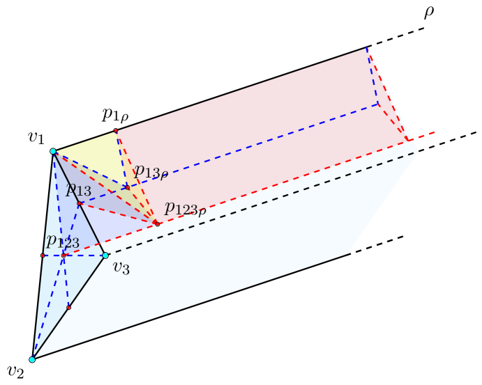
The barycentric subdivision of is defined as follows. The vertex set of is the collection of the barycenters one for each in . A chain in of length is a collection of elements . Given a subset , a chain in of length is a collection of nonempty subsets of . For , we get the empty chain with no element. To each pair consisting of a chain in of some length and a chain in of some length , we associate the polyhedron defined by taking the convex-hull in of the points and all the rays . Then, is the collection of all the polyhedra , see Figures 1 and 2.
Note that for each vertex , we have , so that we get an inclusion . It is easy to check that the recession fan of is the barycentric subdivision of the recession fan of . Denote by the set of recession rays of . We have .
Denote by the partial order on defined by the inclusion of faces. It is described as follows. Given elements and , we have provided that
-
•
is included in , that is, each element coincides with an element in , and
-
•
we have , that is, each element coincides with an element in .
We next embed , preserving its integral structure. Let denote a collection of elements , one for each . The embedding of will be defined in , with integral structure given by the lattice . First, we define the map
Specifically, if with and , then we set .
For each pair with a chain of length in and a chain of length in , let denote the convex hull in of the points and the rays . Using linear interpolation, we extend to a bijective map
for each pair as above.
Let be the collection of the polyhedra , where is a chain in and is a chain in . Note that forms a subcomplex of the product where is the simplex in obtained as the convex hull of the points for . It follows directly from this observation that is an integral -affine polyhedral complex in .
Proposition 5.1.
Notation as above, the maps glue together to define a bijective map . Moreover, under this bijection, the recession fan of is identified with the recession fan of .
The maps and its inverse preserve the integral affine structures. In particular, we have .
Proof.
The first assertion is straightforward. To show that and its inverse preserve the integral structure, it suffices to prove that each map
is induced from an isomorphism between the lattice of and the lattice of . Let and denote the former and the latter lattices, respectively.
Write , with , where and . Write .
Let be the least common multiple of and for each pair . The lattice is generated by the vectors
Similarly, the lattice is generated by the vectors
The map is the restriction of a linear map from the vector space spanned by and to the vector space spanned by and . This map is defined by and . It is straightforward to verify that and its inverse are both integral maps. This establishes the preservation of the integral structure and proves the second statement in the proposition. The final assertion follows immediately as a consequence of the first two statements. ∎
Note that the embedding of induces an embedding of the recession fan of as a subfan of the fan corresponding to the positive orthant . Denote by the recession fan of .
Proposition 5.2.
There exists an integral -affine polyhedral complex structure on that contains as a polyhedral subcomplex, and has a recession fan which is a completion of to a complete fan in . Additionally, we can choose to be convex with a convex recession fan .
Proof.
As observed, is a polyhedral subcomplex of the product , where is the simplex with vertices for . We extend to a convex, integral -affine polyhedral complex structure on the entire space , ensuring that it has a convex recession fan.
Similarly, the positive orthant is a polyhedral subcomplex of the polyhedral complex formed by all the orthants, which is also convex. The product of these polyhedral complex structures on and yields a polyhedral complex structure with the desired properties stated in the proposition. ∎
We fix a polyhedral tubular neighborhood of in , which deformation retracts to via a facewise affine map.
Next, we select a family of integral -affine polyhedral complexes with support , such that:
-
•
Each is a simplicial refinement of ;
-
•
For each , there exists a strictly convex function ; and
-
•
For any refinement of , there exists an such that is a refinement of .
Furthermore, by restricting to a suitable subfamily if necessary, we can assume without loss of generality that every face of intersecting lies entirely within .
For each , let denote the induced subdivision of from . Thus, we have and
We define as the union of all faces of that have nonempty intersection with . It follows from the assumption made above that .
Proposition 5.3.
Each facewise affine function on can be expressed as the difference of two strictly convex facewise affine functions and on . Moreover, if , we can choose and such that both and belong to .
Proof.
For sufficiently large , the functions and are both strictly convex. This proves the first part of the proposition.
To prove the second part, we observe that since , the restriction belongs to . Therefore, we conclude that both and are elements of , as required. ∎
Let be any strictly convex facewise affine function on such that the restriction belongs to . For each , we choose an affine function such that , and for all . Moreover, since , we can assume that is integral -affine for all .
Proposition 5.4.
Notation as above, we have
Proof.
The inequality is straightforward. Indeed, let , and suppose for . Then,
Similarly, we have .
For the reverse inequality, we use the lemma below which asserts that a facewise affine function on that is convex according to Definition 2.3 is also convex as a real-valued function on . We claim that for each , we have globally on .
Fix a point in the relative interior of . Let be any point of , and consider the segment . The restriction is convex, and the restriction of to is affine. There exists a small segment containing such that , with . The function is convex, it takes value zero at , and is non-negative on . We conclude that is non-negative everywhere, i.e., . This gives .
Thus, we obtain both inequalities and . ∎
Lemma 5.5.
Let be a polyhedral complex with support . Let be a facewise affine function on . The following properties are equivalent:
-
(1)
is convex according to Definition 2.3.
-
(2)
is convex as a real-valued function on .
Proof.
The result is well-known, and we provide only a sketch of the proof.
To show (1) implies (2), take a segment in . It will be enough to show that is convex. Since is a piecewise affine function, Definition 2.3 ensures that at points of where there is a change of slopes, the sum of outgoing slopes is positive, which proves the convexity.
To prove the other direction, consider the upper-graph of , defined as the set of all points with . Since is convex, is a convex subset of .
Let be a point in the relative interior of a face of . There exists an affine hyperplane passing through such that the upper-graph of is entirely above . Since is affine, we can assume that contains the affine space generated by . Thus, is of the form for an affine function on . We have , and the inequalities hold for all , as required. ∎
5.1. Proof of Theorem 1.2
Taking the barycentric subdivision of as above, we embed as an integral -affine polyhedral complex in some linear space , with the notation introduced above. We also keep the notation for , , . Let be the fixed retraction map induced from the polyhedral tubular neighborhood of to .
Note that we have for all . We prove is generated over by the restriction of coordinate functions of to .
Let be a piecewise integral -affine function. There exists some such that belongs to . Using the retraction map , we extend to an integral facewise -affine function on , i.e., we set .
Let denote the recession fan of .
Next, we extend to a facewise (not necessarily integral -) affine function on . The extension process works as follows.
First, for each ray in , if is parallel to a ray in , we denote by the slope of along any ray of parallel to . This is well-defined because .
Then, for rays of which are not parallel to any ray in , we set .
We define for every vertex of not contained in .
Once the values of at the vertices of each polyhedron in and the slopes along the rays of are fixed, since is simplicial, we can extend by linear interpolation to the entire polyhedron . This way, we obtain an element . Note that the restriction is integral -affine.
By Proposition 5.3, we can write for strictly convex functions and on such that the restrictions and both belong to . By Proposition 5.4, we can express and as
where are integral -affine functions on with
for all .
From the above, we conclude that belongs to the semifield generated by and the restriction of the coordinate functions of to . Thus, the theorem is proven. ∎
5.2. Proof of Theorem 1.4
To prove the first statement, using the work by Ewald and Ishida [EI06], we extend to an integral -affine polyhedral complex with full support which verifies the properties stated in Proposition 5.2. The rest of the arguments leading to the proof of Theorem 1.2 remains unchanged and gives the first part of Theorem 1.4.
We prove the second part. For a subset of , let
Then, is a congruence on . It is proved in [Son24] that the following are equivalent:
-
(i)
is a finitely generated congruence.
-
(ii)
is the support of an integral -affine polyhedral complex.
(The result is stated over in loc.cit., but the same proof works over .)
Consider the map from the introduction. The kernel of is by definition equal to . Since verifies (ii), is a finitely generated congruence. ∎
5.3. Proof of Theorem 1.3
Let be a smooth projective variety over with a strictly semistable pair . As before, we denote by the dual complex of with the set of vertices and the set of rays , and we identify with .
Let
be the map in Proposition 5.1, so that is bijective and that both and preserve the integral -affine structures. Here, is a subdivision of with the same recession fan, and we have .
Let be the coordinate functions on , where . We define . Then we have . Since is generated by over by Theorem 1.2, is generated by over .
References
- [AI22] Omid Amini and Hernan Iriarte. Geometry of higher rank valuations. arXiv preprint arXiv:2208.06237, 2022.
- [Ber90] Vladimir G. Berkovich. Spectral theory and analytic geometry over non-Archimedean fields, volume 33 of Mathematical Surveys and Monographs. American Mathematical Society, Providence, RI, 1990.
- [Ber99] Vladimir G. Berkovich. Smooth -adic analytic spaces are locally contractible. Invent. Math., 137(1):1–84, 1999.
- [Ber04] Vladimir G. Berkovich. Smooth -adic analytic spaces are locally contractible. II. In Geometric aspects of Dwork theory. Vol. I, II, pages 293–370. Walter de Gruyter, Berlin, 2004.
- [BFJ16] Sébastien Boucksom, Charles Favre, and Mattias Jonsson. Singular semipositive metrics in non-Archimedean geometry. J. Algebraic Geom., 25(1):77–139, 2016.
- [BGS11] José Ignacio Burgos Gil and Martín Sombra. When do the recession cones of a polyhedral complex form a fan? Discrete & Computational Geometry, 46(4):789–798, 2011.
- [BPR16] Matthew Baker, Sam Payne, and Joseph Rabinoff. Nonarchimedean geometry, tropicalization, and metrics on curves. Algebr. Geom, 3(1):63–105, 2016.
- [BR15] Matthew Baker and Joseph Rabinoff. The skeleton of the Jacobian, the Jacobian of the skeleton, and lifting meromorphic functions from tropical to algebraic curves. International Mathematics Research Notices, 2015(16):7436–7472, 2015.
- [Car21] Dustin Cartwright. A specialization inequality for tropical complexes. Compos. Math., 157(5):1051–1078, 2021.
- [CHW14] Maria Angelica Cueto, Mathias Häbich, and Annette Werner. Faithful tropicalization of the Grassmannian of planes. Mathematische Annalen, 360:391–437, 2014.
- [CM19] Maria Angelica Cueto and Hannah Markwig. Tropical geometry of genus two curves. Journal of Algebra, 517:457–512, 2019.
- [DHLY24] Antoine Ducros, Ehud Hrushovski, François Loeser, and Jinhe Ye. Tropical functions on a skeleton. Journal de l’École Polytechnique, 11:613–654, 2024.
- [dJ96] A. J. de Jong. Smoothness, semi-stability and alterations. Inst. Hautes Études Sci. Publ. Math., (83):51–93, 1996.
- [DP16] Jan Draisma and Elisa Postinghel. Faithful tropicalisation and torus actions. Manuscripta Mathematica, 149:315–338, 2016.
- [Duc12] Antoine Ducros. Espaces de Berkovich, polytopes, squelettes et théorie des modèles. Confluentes Mathematici, 4(4), 2012.
- [EI06] Günter Ewald and Masa-Nori Ishida. Completion of real fans and Zariski–Riemann spaces. Tohoku Mathematical Journal, Second Series, 58(2):189–218, 2006.
- [GRW16] Walter Gubler, Joseph Rabinoff, and Annette Werner. Skeletons and tropicalizations. Advances in Mathematics, 294:150–215, 2016.
- [Har01] Urs T Hartl. Semi-stability and base change. Archiv der Mathematik, 77(3):215–221, 2001.
- [Hel19] Paul Alexander Helminck. Faithful tropicalizations of elliptic curves using minimal models and inflection points. Arnold Mathematical Journal, 5(4):401–434, 2019.
- [HW93] Udo Hebisch and Hanns Joachim Weinert. Semirings: algebraic theory and applications in computer science, volume 5. World Scientific, 1993.
- [JM12] Mattias Jonsson and Mircea Mustaţă. Valuations and asymptotic invariants for sequences of ideals. Annales de l’Institut Fourier, 62(6):2145–2209, 2012.
- [KMM08] Eric Katz, Hannah Markwig, and Thomas Markwig. The j-invariant of a plane tropical cubic. Journal of Algebra, 320(10):3832–3848, 2008.
- [Kut16] Max B Kutler. Faithful tropicalization of hypertoric varieties. arXiv preprint arXiv:1604.08271, 2016.
- [KY19] Shu Kawaguchi and Kazuhiko Yamaki. Effective faithful tropicalizations associated to adjoint linear systems. Int. Math. Res. Not. IMRN, (19):6089–6112, 2019.
- [KY21] Shu Kawaguchi and Kazuhiko Yamaki. Effective faithful tropicalizations associated to linear systems on curves, volume 270 of Memoirs of the AMS. American Mathematical Society, 2021.
- [Mat80] Hideyuki Matsumura. Commutative algebra, volume 56 of Mathematics Lecture Note Series. Benjamin/Cummings Publishing Co., Inc., Reading, MA, second edition, 1980.
- [MN15] Mircea Mustaţă and Johannes Nicaise. Weight functions on non-Archimedean analytic spaces and the Kontsevich-Soibelman skeleton. Algebr. Geom., 2(3):365–404, 2015.
- [MRS23] Hannah Markwig, Lukas Ristau, and Victoria Schleis. Faithful tropicalization of hyperelliptic curves. arXiv preprint arXiv:2310.02947, 2023.
- [Ran17] Dhruv Ranganathan. Skeletons of stable maps I: rational curves in toric varieties. Journal of the London Mathematical Society, 95(3):804–832, 2017.
- [Son24] JuAe Song. Finitely generated congruences on tropical rational function semifields. arXiv preprint arXiv:2405.14087, 2024.