Uniformly Expanding Full Branch Maps with a Wild Attracting Point

Abstract.

We give a counterintuitive example of a uniformly expanding full branch map such that the point zero is a wild attractor.

1. Introduction and Main Result

For any dynamical system $f:M\to M$ defined on a manifold $M$, define the basin of attraction of a point $p$ as follows:

$$B_{p}:=\{x|f^{n}(x)\xrightarrow[]{n\to\infty}p\}.$$

There are two different notions of an attractor, based on two different notions of size for a set. If $B_{p}$ is residual on an open subset of $M$, then $p$ is a topological attractor. If $B_{p}$ has positive Lebesgue measure, then $p$ is a metric attractor. These notions were first posited in [1]. These two notions often coincide, but not always. A metric attractor that is not a topological attractor is called a wild attractor. The existence of a wild Cantor attractor was proven in [2] for a polynomial unimodal map. In this paper we prove the following existence result.

Theorem 1.1 (Main Theorem).

There exists $f:[0,1]\to[0,1]$ a uniformly expanding full branch map with countably infinite branches that are each $C^{\infty}$, such that $B_{0}$ is a meagre set and

$$|B_{0}|=1.$$

Thus the point $0$ is a wild attractor.

As a consequence, $\delta_{0}$ is the unique physical measure of $f$. Furthermore by the Poincare recurrence theorem, any invariant measure of $f$ must be singular with respect to the Lebesgue measure. Therefore $f$ has no ACIP. Another example of a uniformly expanding full branch map without ACIP was presented in [3], which has finitely many branches but required a lower regularity ($C^{1}$) on each branch.

Before we define precisely our setting of uniformly expanding full branch maps, we begin with a nontechnical discussion on the role of contraction and expansion in dynamical systems. Contraction typically gives us dynamics that are more simple. By the Banach fixed point theorem, a contraction mapping on a metric space gives a unique globally attracting fixed point, which is a very simple dynamics.

On the other hand, expansion typically gives us systems that are more chaotic. One famous result for expanding maps is the folklore theorem on expanding circle maps. Let $f$ be an expanding circle endomorphism with $C^{2}$ regularity, then $f$ admits a unique ergodic invariant probability measure $\mu$ which is equivalent to Lebesgue measure. As a consequence, the orbit of a typical point will spread around the space in a dense and chaotic way, visiting each open set with positive frequency. This is not true for lower regularity, in fact for a generic $C^{1}$ expanding circle map there is a unique physical measure which is singular with respect to Lebesgue measure [4]. But the singular measure is still fully supported, so the orbit of a typical point will still visit every open set with a positive frequency. Expanding circle maps also have a natural generalization as full branch maps. We now define our setting of uniformly expanding full branch maps.

Definition 1.1 (Full Branch Map).

Given a bounded closed interval $I$ with a modulo $0$ partition $\mathcal{P}$ (finite or countably infinite), a full branch map is a map $f:I\to I$ such that $\forall J\in\mathcal{P},f:\mathring{J}\to\mathring{I}$ is a homeomorphism.

Each partition element $J$ together with the restriction $f|_{J}$ is called a branch. An iterate of a full branch map $f^{n}$ is also a full branch map, with a new partition denoted $\mathcal{P}_{n}$.

Definition 1.2 (Uniformly Expanding Full Branch Map).

A full branch map is called uniformly expanding if there exists a constant of expansion $\lambda>1$ with another constant $C\in\mathbb{R}$ such that for all $n\geq 1$, for all $x$ where ${f^{n}}^{\prime}(x)$ is defined:

$${f^{n}}^{\prime}(x)\geq C\lambda^{n}.$$

Note that a sufficient condition for uniform expansion with $C=1,\lambda>1$ is $f^{\prime}(x)\geq\lambda$ where it is defined.

We now discuss several results on the physical measures of uniformly expanding full branch maps. Typically they begin with assumptions that imply some form of bounded distortion, which is an upper bound on the quantity

$$\sup_{I\in\mathcal{P}^{n}}\sup_{x,y\in I}|f^{\prime}(x)|/|f^{\prime}(y)|.$$

This bound is then applied to obtain a unique ergodic invariant probability measure $\mu$ which is equivalent to Lebesgue measure. For a map with finitely many branches, we have a generalization of the folklore theorem. If $f$ has $C^{2}$ regularity on each branch, then $f$ admits a unique ergodic invariant probability measure $\mu$ which is equivalent to Lebesgue measure. For a map with infinite branches, bounded distortion is given by the Adler condition [5]. $f$ has the Adler condition if:

$$\sup_{I\in\mathcal{P}}\sup_{x,y\in I}|f^{\prime\prime}(x)|/|f^{\prime}(y)|^{2}<\infty.$$

If a uniformly expanding map satisfies the Adler condition, then it admits a unique ergodic invariant probability measure $\mu$ which is equivalent to Lebesgue measure. One famous example of a map satisfying it is the Gauss continued fraction map, defined as $f(x):=1/x\mod 1$, which admits the following invariant measure $\mu(E):=1/(\log 2)\int_{E}1/(1+x)dx$.

Theorem 1.1 is an example of the counterintuitive behavior that we can obtain on uniformly expanding full branch maps without bounded distortion. It shows us how the topological chaos of uniform expansion can coexist with the metric attraction on a full measure basin.

2. Outline of Proof

For this paper, we consider $f:[0,1]\to[0,1]$ to be a full branch map with countably infinite branches, with the following structure and labeling of branches:

• There exists a strictly decreasing sequence $(a_{n})_{n=1}^{\infty}$ such that $a_{1}=1$ and $a_{n}\xrightarrow[]{n\to\infty}0$

• $I_{n}:=]a_{n+1},a_{n}]$

• $f:I_{n}\to]0,1]$ are orientation preserving homeomorphisms.

• $f(0)=0$.

We now define some more subsets of $]0,1]$.

$$\widehat{I_{n}} :=\bigcup_{k\geq n}I_{k}=]0,a_{n}], I_{n}$$ i.e. the union of and branches to its left.

$$L_{n} :=I_{n}\cap f^{-1}(\widehat{I_{n+1}}), I_{n}$$ i.e. the subinterval of that maps to its left.

Note that $f:L_{n}\to\widehat{I_{n+1}}$ is a homeomorphism. Because $f|_{I_{n}}$ is orientation preserving, $L_{n}$ shares the left endpoint of $I_{n}$. Visually, these $L_{n}$ are mapped below the diagonal, which means they get mapped closer to $0$. We are naturally interested in how large $L_{n}$ is compared to $I_{n}$ in terms of Lebesgue measure. So we define the sequence of proportions $(p_{n})_{n=1}^{\infty}$ and its product as follows:

$$p_{n}:=\frac{|L_{n}|}{|I_{n}|},\quad P:=\prod_{n\geq 1}p_{n}.$$

We will prove in Section 3 the following result:

Proposition 2.1.

For any $f$, $B_{0}$ is a meagre set.

In this paper we define an important property for $f$, called subdiagonal structure property (SSP). This property essentially says that a large majority of points are mapped to the left by the subintervals $L_{n}$.

Definition 2.1 (Subdiagonal Structure Property (SSP)).

A map $f$ has SSP if it satisfies the following:

• Every branch $f|_{I_{n}}:I_{n}\to]0,1]$ is convex.

• $(p_{n})$ is an increasing sequence.

• $P>0$.

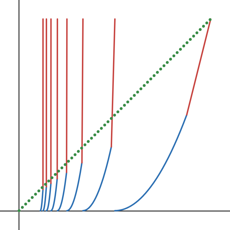
Figure 1. Example of map with SSP

In Section 6 we will obtain the following result.

Theorem 2.1.

Let $f$ be a map with SSP. Then:

$$|B_{0}|=1.$$

Also observe that SSP is a $C^{0}$ notion that is defined independently from regularity and expansion assumptions. So we still need to show that SSP is compatible with branchwise $C^{\infty}$ regularity and uniform expansion. In Section 7 we will obtain the following result.

Theorem 2.2.

There exists a map $f$ with SSP, such that $f$ is uniformly expanding and each branch is $C^{\infty}$.

The main Theorem 1.1 is a consequence of applying Proposition 2.1 and Theorem 2.1 to the map $f$ obtained from Theorem 2.2.

3. Topology of Basin

Let $f$ be a map, with or without SSP. In this section we show that $B_{0}$ is meagre. The key observation here is the fact that $f$ is a uniformly expanding full branch map, thus it is locally eventually onto. First we define the sets $D_{n}$ to be set of points that do not recur to $I_{1}$ after time $n$, and $D$ to be the set of points that eventually do not recur to $I_{1}$:

$$D_{n} :=\{x|\forall k\geq n,f^{k}(x)\notin I_{1}\}$$

$$D :=\bigcup_{n\geq 1}D_{n}$$

Because $I_{1}$ is not a neighborhood of $0$, points that converge to $0$ must eventually not recur to $I_{1}$. Therefore, $B_{0}\subset D$.

Lemma 3.1.

$D$ is a meagre set.

Proof.

Fix any time $n$. Fix any open interval $J$. Because $f$ is a uniformly expanding full branch map, it is locally eventually onto. So there must be a sufficiently large time $m\geq n$ and a subinterval $J^{\prime}\subset J$ that is homeomorphic by $f^{m}$ to $I_{1}$. Thus $D_{n}$ is nowhere dense. Therefore the countable union $D$ is a meagre set. ∎

Because $B_{0}\subset D$, by Lemma 3.1 $B_{0}$ is a meagre set. Thus we obtain Proposition 2.1.

4. Symbolic Dynamics

Let $f$ be a map, with or without SSP. We will study the itineraries of points. For a point $x$ in a full branch map, its itinerary is the sequence of indices of the branch that $x$ visits in any given time. In particular for our setting:

$$\forall x\in]0,1],\quad\exists(k_{i})_{i=0}^{\infty}:f^{i}(x)\in I_{k_{i}}$$

Define $C$ to be the set of points with itineraries that are strictly increasing:

$$C:=\{x|\forall i\geq 0,k_{i}<k_{i+1}\}.$$

Note that $C\subset B_{0}$. We also define the set $E$ to be the set of points with itineraries that have strictly increasing tails.

$$E:=\{x|\exists N:\forall i\geq N,k_{i}<k_{i+1}\}.$$

Also note that $E\subset B_{0}$. We can also interpret $E$ as the set of points that eventually fall into $C$.

In Section 5 we will estimate the measure of preimages of $C$, and in Section 6 we will show $E$ has full measure, which proves Theorem 2.1.

4.1. C as a nested intersection of $C_{n}$

We now study the set $C$ in greater detail. We will view $C$ as a nested intersection of decreasing sets $C_{n}$, and each $C_{n}$ is defined using branches of iterations of $f$. We will conclude with two Lemmas 4.1 and 4.2, to describe the nesting of $C_{n+1}\subset C_{n}$ in terms of left subintervals of branches.

First, recall that a full branch map $f$ is associated with a partition of branches $\mathcal{P}$. In our case,

$$\mathcal{P}=\{I_{1},I_{2},I_{3},...\}.$$

$\forall n\geq 1$, $f^{n}$ is also a full branch map, so we also have $\mathcal{P}_{n}$, the partition of $I$ into the branches of $f^{n}$. Also note that each member of $\mathcal{P}_{n+1}$ is an intersection that is obtained by an itinerary from time $0$ to $n$.

$$\mathcal{P}_{n+1}=\{J|\exists(k_{i})_{i=0}^{n}:J=(I_{k_{0}})\cap f^{-1}(I_{k_{1}})\cap...\cap f^{-n}(I_{k_{n}})\}$$

For brevity, we use the notation for cylinder sets from symbolic dynamics. Given an itinerary up to time $n$, i.e. $(k_{i})_{i=0}^{n}$, we define:

$$[k_{0},k_{1},...,k_{n}]:=(I_{k_{0}})\cap f^{-1}(I_{k_{1}})\cap...\cap f^{-n}(I_{k_{n}}).$$

We define $C_{n}$ as the union of branches which have strictly increasing itinerary up to time $n$.

$$C_{n}:=\bigcup_{1\leq k_{0}<k_{1}<...<k_{n}}[k_{0},k_{1},...,k_{n}].$$

Observe that $(C_{n})$ is a nested decreasing sequence of sets. Also by definition, $C_{n}$ is the set of points whose itineraries increase up to time $n$. So by definition of $C$:

$$C=\bigcap_{n\geq 1}C_{n}.$$

We know the sets $C_{n}$ are nested, but we need to understand the structure of the nesting better. We begin by the following observation that $C_{1}$ is also the union of the left subintervals of the branches of $C_{0}$.

$$C_{0} =\bigcup_{1\leq k_{0}}[k_{0}]=\bigcup_{1\leq k_{0}}I_{k_{0}}.$$

$$C_{1} =\bigcup_{1\leq k_{0}<k_{1}}[k_{0},k_{1}]=\bigcup_{1\leq k_{0}}\bigcup_{k_{0}<k_{1}}[k_{0},k_{1}]=\bigcup_{1\leq k_{0}}\bigcup_{k_{0}<k_{1}}I_{k_{0}}\cap f^{-1}(I_{k_{1}})$$

$$=\bigcup_{1\leq k_{0}}\left[I_{k_{0}}\cap\bigcup_{k_{0}<k_{1}}f^{-1}(I_{k_{1}})\right]=\bigcup_{1\leq k_{0}}\left[I_{k_{0}}\cap f^{-1}(\widehat{I_{k_{0}+1}})\right]=\bigcup_{1\leq k_{0}}L_{k_{0}}.$$

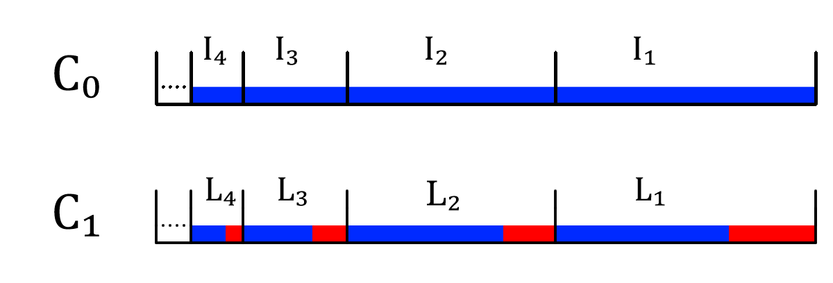
Figure 2. How $C_{1}$ is nested inside $C_{0}$.

To extend this observation, we need a generalization of the left subintervals $L_{k}\subset I_{k}$. We will define the left subinterval of a branch of higher iterate. Take a branch $[k_{0},...,k_{n}]$ contained in $C_{n}$. We collect the subbranches whose index increases at time $n+1$, and take their union:

$$L([k_{0},k_{1},...,k_{n}]):=\bigcup_{k_{n}<k_{n+1}}[k_{0},k_{1},...,k_{n},k_{n+1}].$$

Note that $L([k_{0},k_{1},...,k_{n}])\subset[k_{0},k_{1},...k_{n}]$ as a left subinterval. Now we observe two important lemmas that explain this nesting in terms of left subintervals:

Lemma 4.1 (Partition lemma).

Take any $n\geq 1$. Then we can partition $C_{n+1}$ by the left subintervals of $C_{n}$:

$$C_{n+1}=\bigcup_{1\leq k_{0}<...<k_{n+1}}[k_{0},k_{1},...,k_{n},k_{n+1}]=\bigcup_{1\leq k_{0}<...<k_{n}}L([k_{0},k_{1},...,k_{n}]).$$

Proof.

The first equation is true by definition of $C_{n+1}$. The second equation is true by definition of $L([k_{0},k_{1},...,k_{n}])$. ∎

Lemma 4.2 (Image of left subinterval).

Take any branch $[k_{0},k_{1},...,k_{n}]$. Then:

$$f^{n}:[k_{0},k_{1},...,k_{n}] \to I_{k_{n}}$$ is a homeomorphism by definition, and

$$f^{n}:L([k_{0},k_{1},...,k_{n}]) \to L_{k_{n}}$$ is also a homeomorphism.

Proof.

Because a restriction of a homeomorphism is a homeomorphism, we only need to compute the image.

$$f^{n}(L([k_{0},k_{1},...,k_{n}])) =\bigcup_{k_{n}<k_{n+1}}f^{n}([k_{0},k_{1},...,k_{n},k_{n+1}])=\bigcup_{k_{n}<k_{n+1}}[k_{n},k_{n+1}]=L_{k_{n}}.$$

∎

By the Lemmas 4.1 and 4.2 we can now picture how $C_{n+1}$ is nested in $C_{n}$.

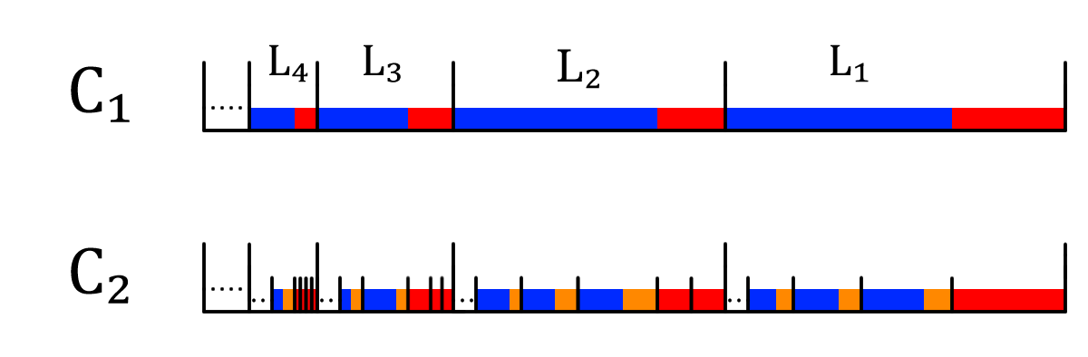
Figure 3. How $C_{2}$ is nested inside $C_{1}$.

5. SSP and Convex Preimages of $C$

In the previous Section 4, given a map $f$, we can define the set $C$. The key technical idea of this paper is to use the assumptions of SSP to give a lower bound for the Lebesgue measure of preimages of $C$ by convex homeomorphisms.

Proposition 5.1.

(Convex Preimages of $C$) Let $f$ be a map with SSP. Let $C$ be the set defined by $f$. Take any bounded interval $J$ such that there exists a convex orientation preserving homeomorphism $g:J\to]0,1]$. Then $\forall n\geq 1$:

$$|g^{-1}(C_{n})|\geq|J|\prod_{i=1}^{n}p_{i}.$$

And because $C$ is the nested intersection of $C_{n}$,

$$|g^{-1}(C)|\geq|J|P.$$

We begin with an elementary observation for preimages of left subintervals.

Lemma 5.1 (Convex Preimages of Left Subintervals).

Let $J,I$ be bounded intervals. Let $f:J\to I$ be a convex orientation preserving homeomorphism. Let $L$ be a left subinterval of $I$ (i.e. they share a left endpoint.) Then the proportion of Lebesgue measure contained in the subinterval increases by preimage:

$$\frac{|f^{-1}(L)|}{|J|}=\frac{|f^{-1}(L)|}{|f^{-1}(I)|}\geq\frac{|L|}{|I|}.$$

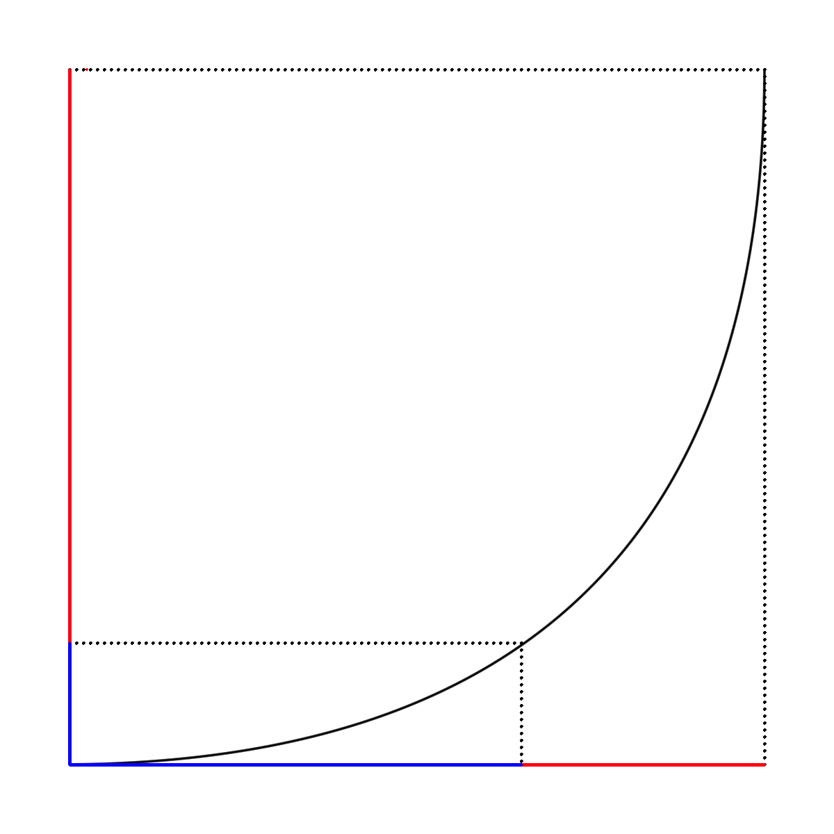
Figure 4. Visual Proof of Lemma 5.1

We now prove the Proposition 5.1.

Proof.

Our strategy is to apply Lemma 5.1 with a proof by induction. For the base case $C_{1}$, recall that $C_{1}=\bigcup_{n\geq 1}L_{n}$. We use this decomposition to obtain the estimate:

$$|g^{-1}(C_{1})| =\sum_{n\geq 1}|g^{-1}(L_{n})|$$

$$\geq\sum_{n\geq 1}|g^{-1}(I_{n})|\frac{|L_{n}|}{|I_{n}|}$$ (g is convex, apply Lemma 5.1)

$$=\sum_{n\geq 1}|g^{-1}(I_{n})|p_{n} p_{n}$$ (by definition of )

$$\geq\left(\sum_{n\geq 1}|g^{-1}(I_{n})|\right)p_{1} (p_{n})$$ ( is increasing by SSP)

$$=|J|p_{1}$$

Now we perform the inductive step. Recall the partition for $C_{n}$ by definition, and the alternative partition for $C_{n+1}$ from Lemma 4.1 in Section 5:

$$C_{n}=\bigcup_{k_{0}<...<k_{n}}[k_{0},...,k_{n}],\quad C_{n+1}=\bigcup_{k_{0}<...<k_{n}}L([k_{0},...,k_{n}]).$$

We use the two partitions to obtain the estimate:

$$|g^{-1}(C_{n+1})|$$

$$=\sum_{k_{0}<...<k_{n}}|g^{-1}(L([k_{0},...,k_{n}]))|$$

$$\geq\sum_{k_{0}<...<k_{n}}|g^{-1}([k_{0},...,k_{n}])|\frac{|L([k_{0},...,k_{n}])|}{|[k_{0},...,k_{n}]|}$$ (g is convex, apply Lemma 5.1)

$$\geq\sum_{k_{0}<...<k_{n}}|g^{-1}([k_{0},...,k_{n}])|\frac{|f^{n}(L([k_{0},...,k_{n}]))|}{|f^{n}([k_{0},...,k_{n}])|} f^{n}$$ ( branchwise convex by SSP)

$$\geq\sum_{k_{0}<...<k_{n}}|g^{-1}([k_{0},...,k_{n}])|\frac{|L_{k_{n}}|}{|I_{k_{n}}|}$$ (by Lemma 4.2)

$$=\sum_{k_{0}<...<k_{n}}|g^{-1}([k_{0},...,k_{n}])|p_{k_{n}} p_{k_{n}}$$ (by definition of )

$$\geq\left(\sum_{k_{0}<...<k_{n}}|g^{-1}([k_{0},...,k_{n}])|\right)p_{n+1} k_{n}\geq n+1 (p_{n})$$ (, and is increasing)

$$=|g^{-1}(C_{n})|p_{n+1}$$

$$\geq\left(|J|\prod_{i=1}^{n}p_{i}\right)p_{n+1}=|J|\prod_{i=1}^{n+1}p_{i}.$$

∎

6. Full Measure Basin

Let $f$ be a map with SSP. We begin with a consequence of Proposition 5.1. By letting $J=]0,1]$ and $g$ to be the identity, we obtain:

$$|B_{0}|\geq|C|\geq P>0.$$

Note that $C_{1}$ is obviously not full measure, so $C$ cannot have full measure. To show $B_{0}$ is full measure, we need a way to find elements of $B_{0}$ outside of $C$.

Recall from Section 4 the set $E\subset B_{0}$, and that $E$ is the set of points whose itineraries have strictly increasing tails. We define the complement:

$$D:=]0,1]\setminus E.$$

By negating the definition of $E$, $D$ is the set of points whose itineraries do not have a strictly increasing tail. We can also interpret $D$ as the set of points that do not fall into $C$. To show $|E|=1$, we want to show that $|D|=0$. Our strategy is to express $D$ as the nested intersection of decreasing sets $D_{m}$ which we will define below.

Define $D_{1}:=]0,1]\setminus C$. Define the collection of branches that strictly increase except at the last index.

$$\mathcal{F}_{1}:=\{[k_{0},k_{1},...,k_{n}]|k_{0}<k_{1}<k_{2}<...<k_{n-1},k_{n-1}\geq k_{n}\}.$$

Notice that this collection is pairwise disjoint, and it forms a partition for $D_{1}$:

$$D_{1}=\bigcup_{J\in\mathcal{F}_{1}}J.$$

To obtain $D_{2}$, we want to remove the points of $D_{1}$ that fall into $C$. Let $J\in\mathcal{F}_{1}$ be a branch with time $n$. Because $f^{n}|_{J}:J\to]0,1]$ is a homeomorphism, we can partition $J$ into two disjoint subsets:

$$]0,1]=D_{1}\bigsqcup C\implies J=(f^{n}|_{J})^{-1}{(D_{1})}\bigsqcup(f^{n}|_{J})^{-1}{(C)}$$

We now define $D_{2}$ by the union of preimages of $D_{1}$:

$$D_{2}:=\bigcup_{J\in\mathcal{F}_{1}}(f^{n}|_{J})^{-1}{(D_{1})}$$

(Note that $$n J$$ depends on , but we omit this in the notation for brevity.)

Similar to $D_{1}$, $D_{2}$ is also a union of pairwise disjoint branches. Observe:

$$D_{2} =\bigcup_{J\in\mathcal{F}_{1}}(f^{n}|_{J})^{-1}(D_{1})$$

$$=\bigcup_{J\in\mathcal{F}_{1}}(f^{n}|_{J})^{-1}(\bigcup_{J^{\prime}\in\mathcal{F}_{1}}J^{\prime})$$

$$=\bigcup_{J,J^{\prime}\in\mathcal{F}_{1}}(f^{n}|_{J})^{-1}(J^{\prime}).$$

We collect these new branches in the family $\mathcal{F}_{2}$, and obtain a partition for $D_{2}$.

$$\mathcal{F}_{2} :=\{(f^{n}|_{J})^{-1}(J^{\prime})|J,J^{\prime}\in\mathcal{F}_{1}\}$$

$$D_{2} =\bigcup_{J\in\mathcal{F}_{2}}J.$$

We repeat this process inductively for any $m\geq 1$. Given a set $D_{m}$ and a collection of branches $\mathcal{F}_{m}$ which partitions it, we can obtain them for $m+1$:

$$D_{m+1} :=\bigcup_{J\in\mathcal{F}_{m}}(f^{n}|_{J})^{-1}(D_{1})$$

$$\mathcal{F}_{m+1} :=\{(f^{n}|_{J})^{-1}(J^{\prime})|J\in\mathcal{F}_{m},J^{\prime}\in\mathcal{F}_{1}\}$$

$$D_{m+1} =\bigcup_{J\in\mathcal{F}_{m+1}}J.$$

We also have a symbolic description of these sets. We begin with the branches. Let $J=[k_{0},...,k_{n-1}]$ (note that a branch of time $n$ is defined by an itinerary from time $0$ to $n-1$), and $J^{\prime}=[k_{0}^{\prime}...,k^{\prime}_{n^{\prime}-1}]$, then we obtain the new branch by their concatenation:

$$(f^{n}|_{J})^{-1}(J^{\prime})=[k_{0},...,k_{n-1},k_{0}^{\prime},...,k^{\prime}_{n^{\prime}-1}].$$

So a branch of $\mathcal{F}_{m}$ is a finite concatenation of $m$ branches of $\mathcal{F}_{1}$. Take the nested intersection $\bigcap_{m\geq 1}D_{m}$. It is the set of points whose itinerary is an infinite concatenation of branches of $\mathcal{F}_{1}$. By definition of $\mathcal{F}_{1}$, $\bigcap_{m\geq 1}D_{m}$ is the set of points whose itineraries do not have strictly increasing tails. Therefore:

$$D=\bigcap_{m\geq 1}D_{m}.$$

Now we estimate $|D|$. Denote $\varepsilon:=1-P$. Observe that

$$|D_{1}|=1-|C|\leq 1-P=\varepsilon.$$

Recall that $D_{m+1}$ is obtained from $D_{m}$ by removing convex preimages of $C$. Applying Proposition 5.1, we obtain the following computational lemma:

Lemma 6.1.

$\forall m\geq 1$,

$$|D_{m+1}|\leq\varepsilon|D_{m}|.$$

Proof.

Recall we obtain $D_{m+1}$ by refining the branches of $\mathcal{F}_{m}$. We observe what happens on a branch $J\in\mathcal{F}_{m}$. Let $n$ be the time of $J$. So $f^{n}:J\to]0,1]$ is a strictly increasing homeomorphism. By SSP, $f^{n}|_{J}$ is also convex. So by Proposition 5.1:

$$|(f^{n}|_{J})^{-1}(C)|\geq|J|P$$

We obtain the estimate for $|D_{m+1}|$:

$$|D_{m+1}| =\sum_{J\in\mathcal{F}_{m}}\left|J\cap(f^{n}|_{J})^{-1}(D_{1})\right|$$

$$=\sum_{J\in\mathcal{F}_{m}}(|J|-|(f^{n}|_{J})^{-1}(C)|)$$

$$\leq\sum_{J\in\mathcal{F}_{m}}(|J|-|J|P)$$

$$=\left(\sum_{J\in\mathcal{F}_{m}}|J|\right)(1-P)$$

$$=|D_{m}|(1-P)=|D_{m}|\varepsilon.$$

∎

As a consequence of Lemma 6.1,

$$|D| =\lim_{m\to\infty}|D_{m}|\leq\lim_{m\to\infty}\varepsilon^{m}=0,$$

$$|E| =|1|-|D|=1-0,$$

$$|B_{0}| =|E|=1.$$

We obtain Theorem 2.1.

7. Construction of Example

In this section we will construct a map that satisfies Theorem 2.2. We begin by fixing several parameters, the domains $I_{n}$, and subintervals $L_{n}$. Fix $c\in]1,2[$. We then fix the sequence $a_{n}:=c^{-n+1}$, which automatically fixes the branch domains:

$$I_{n}:=[a_{n+1},a_{n}]=[c^{-n},c^{-n+1}].$$

We also fix the constant of expansion:

$$\lambda\>=\frac{1}{c-1}\geq 1.$$

We now fix the sequence of proportions $(p_{n})_{n\geq 1}$ with an additional requirement that $p_{1}$ is large enough such that:

$$\frac{p_{1}}{1-p_{1}}\geq\lambda.$$

On each depth $n\geq 1$, these proportions $p_{n}$ detemines the left subintervals $L_{n}\subset I_{n}$. Now we need to define the branches $f|_{I_{n}}$. The properties we require are:

• $f|_{I_{n}}$ is a convex orientation-preserving homeomorphism.

• $f|_{I_{n}}$ has $C^{\infty}$ regularity.

• $f^{\prime}|_{I_{n}}\geq\lambda$.

• The left subinterval $L_{n}$ must be mapped to $\widehat{I_{n+1}}$.

• The right subinterval $R_{n}:=I_{n}\setminus L_{n}$ must be mapped to $]0,1]\setminus\widehat{I_{n+1}}$.

The following computational lemma will help us define $f|_{I_{n}}$ in a way that satisfies all the properties:

Lemma 7.1.

$\forall n\geq 1$, we have:

$$\frac{|\widehat{I_{n+1}}|}{|L_{n}|}=\frac{\lambda}{p_{n}},\quad\frac{|]0,1]\setminus\widehat{I_{n+1}}|}{|R_{n}|}\geq\frac{\lambda}{p_{n}}.$$

Proof.

We prove the first item.

$$\frac{|\widehat{I_{n+1}}|}{|L_{n}|} =\frac{|\widehat{I_{n+1}}|}{p_{n}|I_{n}|}=\frac{1}{p_{n}}\frac{a_{n+1}}{a_{n}-a_{n+1}}$$

$$=\frac{1}{p_{n}}\frac{c^{-n}}{c\cdot c^{-n}-c^{-n}}=\frac{1}{p_{n}}\frac{1}{c-1}=\frac{\lambda}{p_{n}}.$$

Now we prove the second item.

$$\frac{|]0,1]\setminus\widehat{I_{n+1}}|}{|R_{n}|} =\frac{1-|\widehat{I_{n+1}}|}{(1-p_{n})|I_{n}|}=\frac{1}{(1-p_{n})}\frac{1-a_{n+1}}{a_{n}-a_{n+1}}$$

$$=\frac{1}{(1-p_{n})}\frac{1-c^{-n}}{c\cdot c^{-n}-c^{-n}}=\frac{1}{(1-p_{n})}\frac{c^{n}-1}{c-1}$$

$$\geq\frac{1}{(1-p_{n})}\frac{c-1}{c-1}=\frac{1}{(1-p_{n})}.$$

Now recall by our choice of $(p_{n})$,

$$\frac{p_{1}}{1-p_{1}}\geq\lambda\implies\frac{p_{n}}{1-p_{n}}\geq\lambda\implies\frac{1}{1-p_{n}}\geq\frac{\lambda}{p_{n}}.$$

Then we obtain:

$$\frac{|]0,1]\setminus\widehat{I_{n+1}}|}{|R_{n}|}\geq\frac{1}{(1-p_{n})}\geq\frac{\lambda}{p_{n}}.$$

∎

We now define $f|_{L_{n}}:L_{n}\to\widehat{I_{n+1}}$ to be affine. By the second item of Lemma 7.1, we can extend it to $I_{n}$ to obtain $f|_{I_{n}}$, such that it maps $R_{n}$ to $]0,1]\setminus\widehat{I_{n+1}}$ and $f^{\prime}(x)$ is smoothly increasing. Which means the branch $f|_{I_{n}}$ is a $C^{\infty}$ convex orientation-preserving homeomorphism. By the first item of Lemma 7.1, the minimum derivative in the branch is $\frac{\lambda}{p_{n}}$, which is greater than $\lambda$.

By defining $f|_{I_{n}}$ in this manner for all branches $I_{n}$, we obtain a map $f$ that is branchwise $C^{\infty}$, uniformly expanding with constant $\lambda$, and has SSP. We conclude Theorem 2.2.

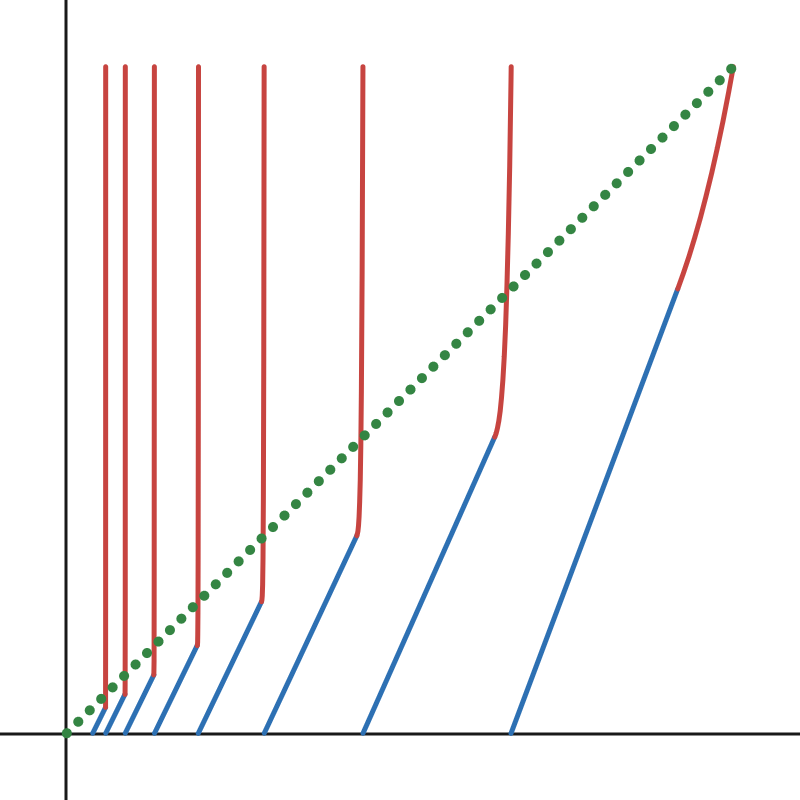
Figure 5. A map $f$ satisfying Theorem 2.2, with $c=1.5$.

For the sake of presenting a dichotomy we have this following lemma.

Lemma 7.2.

Let $f$ be a map with SSP with branchwise $C^{1}$ regularity, such that $a_{n}=c^{-n}$ with $c\in[2,\infty[$. Then $f^{\prime}(x)$ is not uniformly bounded above $1$.

Proof.

Because $f$ has SSP, $p_{n}=\frac{|L_{n}|}{|I_{n}|}$ converges to $1$ as $n\to\infty$. We can now compute the limit of $\frac{|f(L_{n})|}{|L_{n}|}$:

$$\lim_{n\to\infty}\frac{|f(L_{n})|}{|L_{n}|} =\lim_{n\to\infty}\frac{|\widehat{I_{n+1}}|}{|L_{n}|}=\lim_{n\to\infty}\frac{|a_{n+1}|}{|L_{n}|}$$

$$=\lim_{n\to\infty}\frac{a_{n+1}}{p_{n}|I_{n}|}=\lim_{n\to\infty}\frac{1}{p_{n}}\lim_{n\to\infty}\frac{a_{n+1}}{|I_{n}|}$$

$$=1\cdot\lim_{n\to\infty}\frac{a_{n+1}}{|I_{n}|}=\lim_{n\to\infty}\frac{a_{n+1}}{a_{n}-a_{n+1}}$$

$$=\lim_{n\to\infty}\frac{c^{-n}}{c^{-n+1}-c^{-n}}=\lim_{n\to\infty}\frac{c^{-n}}{c\cdot c^{-n}-c^{-n}}$$

$$=\frac{1}{c-1}\leq\frac{1}{2-1}=1.$$

So for any $\varepsilon>0$, there exists $n$ sufficiently large such that

$$\frac{|f(L_{n})|}{|L_{n}|}\leq 1+\varepsilon$$

And by the mean value theorem, there exists $x\in L_{n}$ such that $f^{\prime}(x)\leq 1+\varepsilon$, which means $f^{\prime}(x)$ is not uniformly bounded away from $1$. ∎

References

- [1] John Milnor. On the concept of attractor. Communications in Mathematical Physics, 99(2):177 – 195, 1985.
- [2] H. Bruin, G. Keller, T. Nowicki, and S. van Strien. Wild cantor attractors exist. Annals of Mathematics, 143(1):97–130, 1996.
- [3] P. Gora and B. Schmitt. Un exemple de transformation dilatante et c1 par morceaux de l’intervalle, sans probabilité absolument continue invariante. Ergodic Theory and Dynamical Systems, 9(1):101–113, 1989.
- [4] James T. Campbell and Anthony N. Quas. A generic expanding map has a singular s-r-b measure. Communications in Mathematical Physics, 221(2):335–349, February 2001.
- [5] Roy L. Adler. F-expansions revisited. In Anatole Beck, editor, Recent Advances in Topological Dynamics, pages 1–5, Berlin, Heidelberg, 1973. Springer Berlin Heidelberg.