Gravitational $p\to\Delta^{+}$ transition form factors in chiral perturbation theory

Abstract

The proton to $\Delta^{+}$ resonance transitional gravitational form factors are calculated to leading one-loop order using chiral perturbation theory in our recent work [1]. We take into account the leading electromagnetic and strong isospin-violating effects to obtain non-vanishing contributions. The loop contributions to the transition form factors are found to be free of power-counting violating pieces, which is consistent with the absence of tree-level diagrams at the considered order. Our results involve no free parameters and can be regarded as predictions of chiral perturbation theory.

1 Introduction

Hadrons including proton and neutron are building blocks of our universe. Nevertheless, their fundamental properties, such as mass, spin, and three-dimensional structures are still unclear in many aspects. These properties are closely related to the energy-momentum tensor (EMT) operator. The matrix elements of EMT can be written in terms of the gravitational form factors (GFFs) [2]. At zero momentum transfer, these form factors correspond to the hadron mass, spin, and the so-called D-term which characterizes the distribution of forces inside the particles. Although the D-term is a property as fundamental as the mass and spin, it is much less understood. For a long time, it was believed that the GFFs can be accessed only through the graviton exchange, which is too weak to measure in any practical experiments.

After the introduction of the generalized parton distributions (GPDs) in the ’90s, it was soon realized that the GFFs are the second Mellin moments of the unpolarized GPDs [3]. Since GPDs can be measured in the scattering experiments, their relations to the GFFs open a new window for the study of hadron structures. Unfortunately, due to the low statistics in the previous measurements, the extracted GFFs suffer from large uncertainties. For example, the measurement of the proton D-term by JLab data gives $-2.04\pm 0.14(\text{stat.})\pm 0.33(\text{syst.})$, which leads to a large error band in the calculation of the internal pressure distribution [4]. To live with the large uncertainties, various effective approaches or models based on different assumptions of hadrons have been proposed in the past decades. These very different assumptions coexist within the large uncertainties of the experimental measurements.

Beyond the scope of single particle, the transition processes are also interesting for the study of hadron structures. While the electromagnetic $p\to\Delta^{+}$ transition has been extensively studied over the past two decades on both the theoretical and experimental sides, see, e.g., Refs. [5], the gravitational $p\to\Delta^{+}$ transition form factors (GTFFs) gained attention only since a few years [6]. The GTFFs can also be accessed experimentally through their connection to the transition GPDs [7, 8, 9], obtained by expanding the non-local QCD operators with various quantum numbers. Non-perturbative properties of the nucleon-$\Delta$ transition GPDs have been studied, e.g., by applying the approach of large $N_{c}$ limit of QCD, as discussed in Sec. 2.7 of Ref. [10]. In Ref. [11], the transition GPDs have been connected with the DVCS amplitude within the process $e^{-}N\to e^{-}\gamma\pi N,$ while in Ref. [12] these quantities have been studied using exclusive electroproduction of $\pi^{-}\Delta^{++}$. Recently, a complete definition of the $N\to\Delta$ transition GPDs has been provided in Ref. [13].

In Ref. [6], the matrix element of the symmetric EMT corresponding to the $p\to\Delta^{+}$ transition has been studied for the first time, where a parametrization for the transitions $\frac{1}{2}^{\pm}\to\frac{3}{2}^{\pm}$ and $\frac{1}{2}^{\pm}\to\frac{3}{2}^{\mp}$ has been suggested in terms of five conserved and four non-conserved GTFFs. The first calculations of the GTFFs of the $N\to\Delta$ transition were done in Ref. [14] using the QCD light-cone sum rules. The interpretation and understanding of the GTFFs have generated much interest recently, including the relation with the concept of QCD angular momentum (AM) [15], etc.

For systematic studies of low-energy hadronic processes involving the $\Delta$ resonances and induced by gravity one may rely on the effective chiral Lagrangian for the nucleons, pions, photons and delta resonances in curved spacetime. Effective Lagrangian of pions in curved spacetime has been obtained in Ref. [16], and the GFFs of the pion are considered in Ref. [17]. The leading and subleading effective chiral Lagrangians for nucleons, delta resonances and pions in curved spacetime, along with the calculation of the leading one-loop contributions to the GFFs of the nucleons and the $\Delta$ resonances can be found in Refs. [18, 19] .

In this proceeding we present our calculation in Ref. [1] of the GTFFs of the $p\to\Delta^{+}$ transition in the framework of manifestly Lorentz-invariant chiral perturbation theory (ChPT) up-to-and-including the third order in the small-scale expansion [23]. Since the gravitational interaction respects the isospin symmetry, such kind of processes are possible only if the isospin symmetry is broken, i.e. if $m_{u}\neq m_{d}$ and/or if the electromagnetic interaction is taken into account. We include both effects at the corresponding leading orders to calculate the one-loop contributions to the GTFFs.

This proceeding is organized as follows: In section 2, we specify the relevant terms of the effective Lagrangian in curved spacetime and expression for the parts of the EMT. We calculate the GTFFs of the $p\to\Delta^{+}$ transition in section 3. The results of our calculations are summarized in section 4.

2 Effective Lagrangian in curved spacetime and the energy-momentum tensor

The action corresponding to the leading-order effective Lagrangian for nucleons, pions, photons and delta resonances, interacting with an external gravitational field, can be obtained from the corresponding expressions in flat spacetime [18, 19]. It has the following form:

$$S_{\rm\gamma}^{(2)} = \int d^{4}x\sqrt{-g}\,\biggl{\{}\,-\frac{1}{4}F_{\mu\nu}F^{\mu\nu}+\frac{m_{\gamma}^{2}}{2}A_{\mu}A^{\mu}\biggl{\}},$$ (1)

$$S_{\rm\pi}^{(2)} = \int d^{4}x\sqrt{-g}\,\left\{\frac{F^{2}}{4}\,{\rm Tr}(D_{\mu}U(D^{\mu}U)^{\dagger})+\frac{F^{2}}{4}\,{\rm Tr}(\chi U^{\dagger}+U\chi^{\dagger})\right\}\,,$$ (2)

$$S_{\rm N\pi}^{(1)} = \int d^{4}x\sqrt{-g}\,\biggl{\{}\,\bar{\Psi}\,i\gamma^{\mu}\overset{\leftrightarrow}{\nabla}_{\mu}\Psi-m\bar{\Psi}\Psi+\frac{g_{A}}{2}\,\bar{\Psi}\gamma^{\mu}\gamma_{5}u_{\mu}\Psi\biggr{\}}\,,$$ (3)

$$S_{\Delta\pi}^{(1)} = -\int d^{4}x\sqrt{-g}\biggl{\{}\bar{\Psi}^{i\mu}\,i\gamma^{\alpha}\overset{\leftrightarrow}{\nabla}_{\alpha}\Psi^{i}_{\mu}-m_{\Delta}\,\bar{\Psi}^{i}_{\mu}\Psi^{i\mu}-g^{\lambda\sigma}\left(\bar{\Psi}^{i}_{\mu}i\gamma^{\mu}{\overset{\leftrightarrow}{\nabla}_{\lambda}}\Psi^{i}_{\sigma}+\bar{\Psi}^{i}_{\lambda}i\gamma^{\mu}{\overset{\leftrightarrow}{\nabla}_{\sigma}}\Psi^{i}_{\mu}\right)$$ (4)

$$+i\bar{\Psi}^{i}_{\mu}\gamma^{\mu}\gamma^{\alpha}\gamma^{\nu}\overset{\leftrightarrow}{\nabla}_{\alpha}\Psi^{i}_{\nu}+m_{\Delta}\bar{\Psi}^{i}_{\mu}\gamma^{\mu}\gamma^{\nu}\Psi^{i}_{\nu}+\frac{g_{1}}{2}\,g^{\mu\nu}\bar{\Psi}^{i}_{\mu}u_{\alpha}\gamma^{\alpha}\gamma_{5}\Psi^{i}_{\nu}$$

$$+\frac{g_{2}}{2}\bar{\Psi}^{i}_{\mu}\left(u^{\mu}\gamma^{\nu}+u^{\nu}\gamma^{\mu}\right)\gamma_{5}\Psi^{i}_{\nu}+\frac{g_{3}}{2}\bar{\Psi}^{i}_{\mu}u_{\alpha}\gamma^{\mu}\gamma^{\alpha}\gamma_{5}\gamma^{\nu}\Psi^{i}_{\nu}\biggr{\}}\,,$$

$$S_{\Delta\rm N\pi}^{(1,2)} = \int d^{4}x\sqrt{-g}~\Biggl{\{}-g_{\pi N\Delta}\bar{\Psi}\left(g^{\mu\nu}-\gamma^{\mu}\gamma^{\nu}\right)u_{\mu,i}\Psi_{\nu,i}$$ (5)

$$+d_{3}^{(2)}i\bar{\Psi}f_{+}^{i\mu\nu}\gamma_{5}\gamma_{\mu}\left(g_{\nu\lambda}-\left[z_{n}+\frac{1}{2}\right]\gamma_{\nu}\gamma_{\lambda}\right)\Psi^{i\lambda}+\text{H.c.}\Biggl{\}}\,.$$

where $\Psi^{\mu}_{i}$ represent the $\Delta$ resonances, $\gamma_{\mu}\equiv e_{\mu}^{a}\gamma_{a}$ with $e_{\mu}^{a}$ being the vielbein gravitational fields, $u$ is the matrix of pion fields, etc. More details on the definitions for the building blocks of the effective Lagrangian and the choice of the external sources can be found in Ref. [1]. The mass term ${m_{\gamma}^{2}}\,A_{\mu}A^{\mu}/2$ is introduced to regularize possible infrared divergences (actually no IR divergences here), and the limit $m_{\gamma}\to 0$ should be performed at the end.

As gravity conserves isospin, the $p\to\Delta^{+}$ transition process exists only via the isospin-symmetry breaking effect, including strong interaction and electromagnetic interaction. The leading isospin breaking effects due to the strong interaction is from the mass difference of the iso-multiplets: delta resonances, proton and neutron, and charged and neutral pions. To incorporate different masses, it’s more connivent to work with fields in the physical basis than that in the isospin basis. The explicit relations for two basis is as follows:

$$\Psi = \begin{pmatrix}\Psi_{p}\\ \Psi_{n}\end{pmatrix},\Psi_{\mu,1}=\frac{1}{\sqrt{2}}\begin{pmatrix}\frac{1}{\sqrt{3}}\Delta^{0}_{\mu}-\Delta^{++}_{\mu}\\ \Delta^{-}_{\mu}-\frac{1}{\sqrt{3}}\Delta^{+}_{\mu}\end{pmatrix},~\Psi_{\mu,2}=-\frac{i}{\sqrt{2}}\begin{pmatrix}\frac{1}{\sqrt{3}}\Delta^{0}_{\mu}+\Delta^{++}_{\mu}\\ \Delta^{-}_{\mu}+\frac{1}{\sqrt{3}}\Delta^{+}_{\mu}\end{pmatrix},~\Psi_{\mu,3}=\sqrt{\frac{2}{3}}\begin{pmatrix}\Delta^{+}_{\mu}\\ \Delta^{0}_{\mu}\end{pmatrix}\,,$$

$$\pi^{1} = \frac{1}{\sqrt{2}}\left(\pi^{+}+\pi^{-}\right),\,\pi^{2}=\frac{i}{\sqrt{2}}\left(\pi^{+}-\pi^{-}\right),\,\pi^{3}=\pi^{0}.$$ (6)

After substituting the above definition of the fields into the action, e.g., Eq.  (5), we get the terms relevant for the leading one-loop order contributions to the $p\to\Delta^{+}$ transition:

$$S_{\Delta\rm N\pi}^{(1)} = \int d^{4}x\sqrt{-g}\,\frac{g_{\pi n\Delta}}{F}\Biggl{\{}\bar{\Psi}_{n}\partial_{\mu}\pi^{+}O_{2}^{\mu\nu}\Delta^{-}_{\nu}-\bar{\Psi}_{p}\partial_{\mu}\pi^{-}O_{2}^{\mu\nu}\Delta^{++}_{\nu}+\frac{1}{\sqrt{3}}\left(\sqrt{2}~\bar{\Psi}_{n}\partial_{\mu}\pi^{0}O_{2}^{\mu\nu}\Delta^{0}_{\nu}\right.$$ (7)

$$-\bar{\Psi}_{n}\partial_{\mu}\pi^{-}O_{2}^{\mu\nu}\Delta^{+}_{\nu}+\left.\bar{\Psi}_{p}\partial_{\mu}\pi^{+}O_{2}^{\mu\nu}\Delta^{0}_{\nu}+\sqrt{2}~\bar{\Psi}_{p}\partial_{\mu}\pi^{0}O_{2}^{\mu\nu}\Delta^{+}_{\nu}\right)\Biggl{\}}\,,$$

where $O_{2}^{\mu\nu}=g^{\mu\nu}-\gamma^{\mu}\gamma^{\nu}$.

The electromagnetic interaction also contributes to the mass splittings within iso-multiplets. To obtain the leading isospin breaking effects due to the radiative corrections we do not distinguish between the masses of the isospin partners, i.e. we take $m_{\Delta^{++}}=m_{\Delta^{+}}=m_{\Delta^{0}}=m_{\Delta^{-}}$, and $m_{p}=m_{n}$. The mass difference effect in electromagnetic interaction would be of higher order correction and therefore beyond the accuracy of our consideration. Note that the separation of these contributions is afflicted with some uncertainties [24].

The EMT for bosonic matter fields can be obtained by varying the action $S$ coupled to a weak classical torsionless gravitational background field with respect to the metric $g_{\mu\nu}(x)$ according to

$$T_{\mu\nu}(g,\psi) = \frac{2}{\sqrt{-g}}\frac{\delta S_{\rm m}}{\delta g^{\mu\nu}}\,.$$ (8)

For example, from the action of Eqs. (1), we obtain the EMT terms in flat spacetime:

$$T^{{(2)}}_{\gamma,\mu\nu} = F_{\mu}^{\alpha}F_{\alpha\nu}+m_{\gamma}^{2}A_{\mu}A_{\nu}+\eta_{\mu\nu}\left(\frac{1}{4}F_{\alpha\beta}F^{\alpha\beta}-\frac{m_{\gamma}^{2}}{2}A_{\alpha}A^{\alpha}\right),\,$$ (9)

where $\eta_{\mu\nu}$ is the Minkowski metric tensor with the signature $(+,-,-,-)$.

For the fermionic fields interacting with the gravitational vielbein fields we use the definition [25]

$$T_{\mu\nu}(g,\psi) = \frac{1}{2e}\left[\frac{\delta S}{\delta e^{a\mu}}\,e^{a}_{\nu}+\frac{\delta S}{\delta e^{a\nu}}\,e^{a}_{\mu}\right]\,.$$ (10)

For example, from the action of Eq. (3) we obtain the following terms for the EMT in flat spacetime:

$$T^{{(1)}}_{\rm N,\mu\nu} = \frac{i}{2}\bar{\Psi}\,\gamma_{\mu}\overset{\leftrightarrow}{D}_{\nu}\Psi-\frac{\eta_{\mu\nu}}{2}\biggl{(}\,\bar{\Psi}\,i\gamma^{\alpha}\overset{\leftrightarrow}{D}_{\alpha}\Psi-m\bar{\Psi}\Psi\biggr{)}+\left(\mu\leftrightarrow\nu\right)\,.$$ (11)

The superscripts indicate the orders which are assigned to the corresponding terms of the action. The complete expressions of EMT can be found in Ref. [1].

3 Gravitational transition form factors to one loop

The matrix element of the total EMT for the transition $p\to\Delta^{+}$ can be parameterized in terms of five form factors as follows [6]:

$$\langle\Delta,p_{f},s_{f}|T^{\mu\nu}|N,p_{i},s_{i}\rangle$$ (12)

$$= \bar{u}_{\alpha}(p_{f},s_{f})\Biggl{\{}F_{1}(t)\left(g^{\alpha\{\mu}P^{\nu\}}+\frac{m_{\Delta^{+}}^{2}-m_{p}^{2}}{\Delta^{2}}g^{\mu\nu}\Delta^{\alpha}-\frac{m_{\Delta^{+}}^{2}-m_{p}^{2}}{2\Delta^{2}}g^{\alpha\{\mu}\Delta^{\nu\}}-\frac{1}{\Delta^{2}}P^{\{\mu}\Delta^{\nu\}}\Delta^{\alpha}\right)$$

$$+ F_{2}(t)\left(P^{\mu}P^{\nu}\Delta^{\alpha}+\frac{(m_{\Delta^{+}}^{2}-m_{p}^{2})^{2}}{4\Delta^{2}}g^{\mu\nu}\Delta^{\alpha}-\frac{m_{\Delta^{+}}^{2}-m_{p}^{2}}{2\Delta^{2}}P^{\{\mu}\Delta^{\nu\}}\Delta^{\alpha}\right)$$

$$+ F_{3}(t)\left(\Delta^{\mu}\Delta^{\nu}-\Delta^{2}g^{\mu\nu}\right)\Delta^{\alpha}$$

$$+ F_{4}(t)\left(g^{\alpha\{\mu}\gamma^{\nu\}}+\frac{2(m_{p}+m_{\Delta^{+}})}{\Delta^{2}}g^{\mu\nu}\Delta^{\alpha}-\frac{m_{p}+m_{\Delta^{+}}}{\Delta^{2}}g^{\alpha\{\mu}\Delta^{\nu\}}-\frac{1}{\Delta^{2}}\gamma^{\{\mu}\Delta^{\nu\}}\Delta^{\alpha}\right)$$

$$+ F_{5}(t)\left(P^{\{\mu}\gamma^{\nu\}}\Delta^{\alpha}+\frac{(m_{\Delta^{+}}^{2}-m_{p}^{2})(m_{p}+m_{\Delta^{+}})}{\Delta^{2}}g^{\mu\nu}\Delta^{\alpha}-\frac{m_{p}+m_{\Delta^{+}}}{\Delta^{2}}P^{\{\mu}\Delta^{\nu\}}\Delta^{\alpha}\right.$$

$$- \left.\frac{m_{\Delta^{+}}^{2}-m_{p}^{2}}{2\Delta^{2}}\gamma^{\{\mu}\Delta^{\nu\}}\Delta^{\alpha}\right)\Biggl{\}}\gamma^{5}u(p_{i},s_{i})\,,$$

where $m_{p}$ and $m_{\Delta^{+}}$ are the proton and the $\Delta^{+}$ masses, respectively, $P=\left(p_{f}+p_{i}\right)/2$, $\Delta=p_{f}-p_{i}$ and $t=\Delta^{2}$, and $P^{\{\mu}\gamma^{\nu\}}=P^{\mu}\gamma^{\nu}+P^{\nu}\gamma^{\mu}$. As discussed before, the above matrix element is zero if the isospin symmetry is exact.

To calculate the leading one-loop contributions to the above matrix elements, one needs to organize different contributions according to a systematic expansion, for which we employ the so-called $\epsilon$-counting scheme (also referred to as the small scale expansion) [23] : the soft scale $Q$ is the order of the pion mass, and the chiral orders for the involving quantities are the following,

$$m_{\pi} \sim Q,\quad m_{\pi^{+}}^{2}-m_{\pi^{0}}^{2}\sim Q^{2},\quad\text{$m_{\Delta}$ and $m_{N}$}\sim Q^{0},\quad m_{\Delta}-m_{N}\sim Q^{1},\quad m_{p}-m_{n}\sim Q^{2},\quad$$

$$\nabla_{\mu}\Psi_{(i)} \sim Q^{0},\quad\text{$\mathcal{L}^{(N)}$ vertex}\sim Q^{N},\quad\text{electric charge }e\sim Q^{1},\quad\text{loop momenta}\sim Q^{1},\quad$$

$$t \sim Q^{2},\quad\text{pion lines}\sim Q^{-2},\quad\text{$N$ and $\Delta$ lines}\sim Q^{-1},\quad\text{photon lines}\sim Q^{-2},$$ (13)

where $\mathcal{L}^{(N)}$ is the interaction terms of the Lagrangian with chiral order $N$. The above power counting is realized after performing an appropriate renormalization to the manifestly Lorentz-invariant calculations, for which we choose the EOMS scheme of Refs. [27].

To obtain the one-loop contributions to the GTFFs due to strong isospin-breaking interactions one has to compute 25 diagrams, where there are only 10 topologically differing diagrams and the rest can be obtained by just changing the masses and overall factors. These 10 diagrams are shown in Fig. 1, which give contributions of orders two and three. We have verified that the result of diagrams in Fig. 1 does not contain power counting violating contributions and all ultraviolet divergences can be absorbed into redefinition of the low-energy coupling constants of the effective Lagrangian. The electromagnetic corrections can be obtained by replacing the pion line with the photon line in Fig. 1, which also does not involve power-counting violating terms, and all ultraviolet divergences can be absorbed as in the case of strong isospin-breaking interactions.

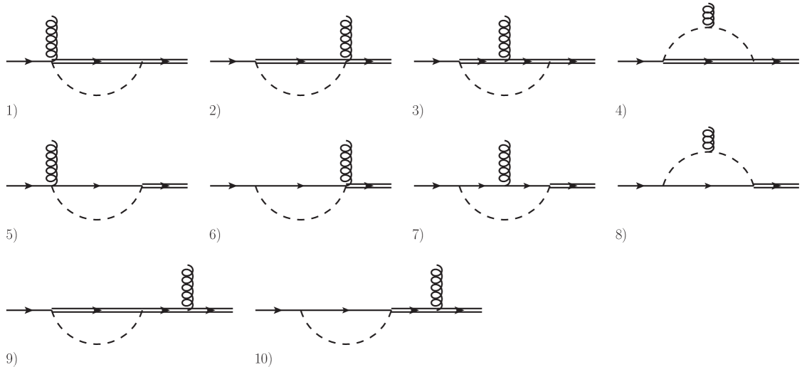
Figure 1: Strong contributions to the gravitational transition form factors. Solid and double lines correspond to nucleons and $\Delta$ resonances, respectively. Dashed lines represent the pions, while the curly lines correspond to gravitons. Initial and final states refer to $p$ and $\Delta^{+}$, respectively, while the baryon lines inside loops refer to propagators of one of the following particles: $\{\Delta^{++},\Delta^{+},\Delta^{0},p,n\}$. Notice that the total contribution of these diagrams vanishes in the limit of exact isospin symmetry.

For the numerical results, we used the following values of the involved parameters:

$$g_{A} = 1.289,\quad g=1.35,\quad m_{\pi^{0}}=0.135,\quad m_{p}=0.938,\quad m_{n}=0.940,\quad$$

$$m_{\Delta} = 1.232,\quad F=0.092,\quad m_{\pi^{+}}=0.140,\quad m_{\Delta^{++}}=1.231,\quad m_{\Delta^{+}}=m_{\Delta},$$

$$m_{\Delta^{0}} = 1.233,\quad g_{1}=9g_{A}/5,\quad e=0.303\,,\quad d_{3}^{(2)}=2.72\,{\rm GeV}^{-1}\,,$$ (14)

where the various masses and the pion decay constant $F$ are given in GeV. In Fig. 2, we present the numerical results of the obtained strong and electromagnetic contributions to the real parts of the transition form factors. There are also imaginary parts which are generated solely by the loop contributions with internal nucleon lines and we do not show them here. The plots demonstrate that the diagrams with radiative corrections give smaller contributions than the ones with pion loops in line with the power counting estimations. On the other hand the groups of diagrams with internal nucleon and delta lines give comparable contributions.

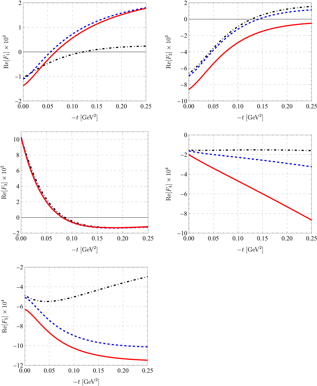
Figure 2: The real parts of the gravitational $p\to\Delta^{+}$ transition form factors. Dash-dotted (black), dashed (blue) and solid (red) lines correspond to the form factors containing contributions of loop diagrams with inner pion and nucleon lines only, diagrams with inner pion and nucleon lines plus radiative corrections, and all loop contributions, respectively.

The leading contributions are given by terms proportional to the pion mass differences. This is because these contributions involve integrals, whose integrands are proportional to

$$\sim\frac{1}{p^{2}-m_{\pi^{+}}^{2}}-\frac{1}{p^{2}-m_{\pi^{0}}^{2}}\simeq\frac{m_{\pi^{+}}^{2}-m_{\pi^{0}}^{2}}{\left(p^{2}-m_{\pi^{+}}^{2}\right)\left(p^{2}-m_{\pi^{0}}^{2}\right)}\,,$$ (15)

and the contributions proportional to the proton-neutron mass difference (analogous for the case of the delta resonances) are given by integrals, whose integrands are proportional to

$$\sim\frac{1}{\not{p}-m_{p}}-\frac{1}{\not{p}-m_{n}}\simeq\frac{m_{p}-m_{n}}{\left(\not{p}-m_{p}\right)\left(\not{p}-m_{n}\right)}\,.$$ (16)

According to the $\epsilon$-counting scheme in (13), the right-hand side of Eq. (15) has chiral order two, the same order as each of the terms in the left-hand side. In contrast, the right-hand side of Eq. (16) has chiral order zero, one order higher than each of the terms on the left-hand side. Therefore the total contribution of diagrams, which is proportional to the proton-neutron mass difference, has the same order as the individual diagrams. While, the total contribution of diagrams, which is proportional to the proton-neutron mass difference squared is suppressed by $Q$. To show it more explicitly, we calculate the real parts of GTFFs with same and different pion masses and only the radiative corrections, given in Fig. 3. As one can see from the plots, for the absolute values of FFs at zero momentum, the case with different pion masses is at least twice as large as the case with same pion masses, and the radiative corrections are much smaller. The numerical result is what we would expect from above analysis. In region of momentum transfer squared that deviates from zero, the radiative corrections give contributions of comparable sizes as the strong isospin violating effects.

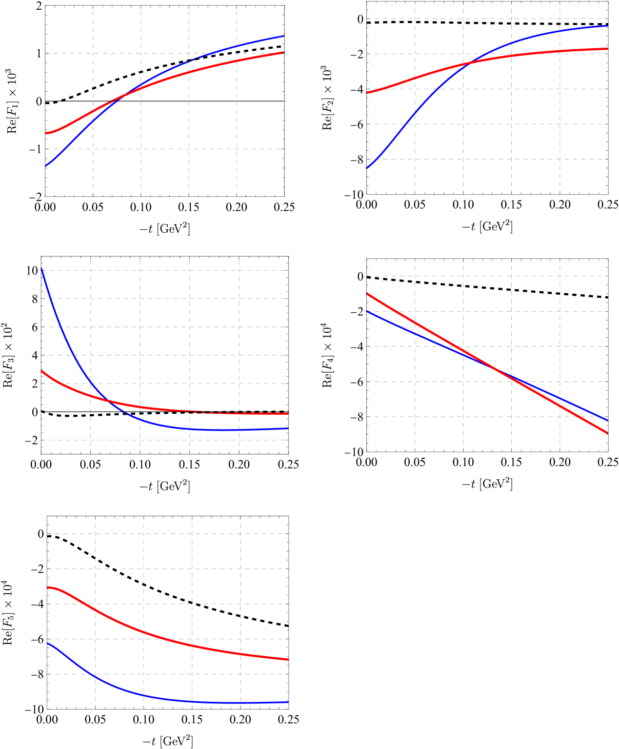
Figure 3: The real parts of the gravitational $p\to\Delta^{+}$ transition form factors with same and different pion masses. The solid (blue), solid (red) and dashed (black) lines correspond to the form factors containing all loop contributions with charged pions having different mass than neutral pion, and that with same pion masses, and the radiative corrections only, respectively.

4 Conclusions and outlook

In the framework of manifestly Lorentz-invariant ChPT for pions, nucleons, photons and the delta resonances interacting with an external gravitational field, we calculated the leading one-loop contributions to the gravitational transition form factors of the $p\to\Delta^{+}$ transition process. As the gravitational interaction respects the isospin symmetry, the amplitude of the $p\to\Delta^{+}$ transition receives non-vanishing contributions due to isospin symmetry breaking. The results of the current work take into account the leading-order electromagnetic and strong isospin-breaking effects. Ultraviolet divergences and power counting violating pieces generated by loop diagrams in the manifestly Lorentz-invariant formulation of ChPT can be treated using the EOMS renormalization scheme. However, at the order of our calculations, the one-loop contributions to the form factors are found to be free of contributions that violate the chiral power counting. This is consistent with the absence of tree-level contributions at the considered order. For this reason, our results involve no free parameters and can be regarded as predictions of ChPT. Notice, however, that the empirical information on the mass splittings between the $\Delta$ resonance states, which enters as an input in our calculations, is presently rather poor. Numerical results for the obtained transition form factors demonstrate that the electromagnetic and strong isospin violating effects give contributions of comparable sizes. This holds true for contributions with both internal nucleon and delta lines.

References

- [1] H. Alharazin, B.-D. Sun, E. Epelbaum, J. Gegelia and U.-G. Meißner, JHEP 03 (2024), 007.
- [2] M. V. Polyakov and P. Schweitzer, Int. J. Mod. Phys. A 33 (2018) no.26, 1830025.
- [3] X. D. Ji, Phys. Rev. Lett. 78 (1997), 610-613.
- [4] V. D. Burkert, L. Elouadrhiri and F. X. Girod, Nature 557 (2018) no.7705, 396-399.
- [5] M. Hilt, T. Bauer, S. Scherer and L. Tiator, Phys. Rev. C 97 (2018) no. 3, 035205.
- [6] J. Y. Kim, Phys. Lett. B 834 (2022), 137442.
- [7] L. L. Frankfurt, M. V. Polyakov and M. Strikman, [arXiv:hep-ph/9808449 [hep-ph]].
- [8] L. L. Frankfurt, M. V. Polyakov, M. Strikman and M. Vanderhaeghen, Phys. Rev. Lett. 84 (2000), 2589-2592.
- [9] S. Diehl, K. Joo, K. Semenov-Tian-Shansky, C. Weiss, V. Braun, W. C. Chang, P. Chatagnon, M. Constantinou, Y. Guo and P. T. P. Hutauruk, et al. [arXiv:2405.15386 [hep-ph]].
- [10] K. Goeke, M. V. Polyakov and M. Vanderhaeghen, Prog. Part. Nucl. Phys. 47 (2001), 401-515.
- [11] K. M. Semenov-Tian-Shansky and M. Vanderhaeghen, Phys. Rev. D 108, no.3, 034021 (2023).
- [12] P. Kroll and K. Passek-Kumerički, Phys. Rev. D 107 (2023) no. 5, 054009.
- [13] J. Y. Kim, K. M. Semenov-Tian-Shansky, H. Y. Won, S. Son and C. Weiss, [arXiv:2501.00185 [hep-ph]].
- [14] U. Özdem and K. Azizi, JHEP 03 (2023), 048.
- [15] J. Y. Kim, Phys. Rev. D 108 (2023) no.3, 034024.
- [16] J. F. Donoghue and H. Leutwyler, Z. Phys. C 52, 343 (1991).
- [17] B. Kubis and U.-G. Meißner, Nucl. Phys. A 671 (2000), 332-356.
- [18] H. Alharazin, D. Djukanovic, J. Gegelia and M. V. Polyakov, Phys. Rev. D 102, no.7, 076023 (2020).
- [19] H. Alharazin, E. Epelbaum, J. Gegelia, U.-G. Meißner and B.-D. Sun, Eur. Phys. J. C 82 (2022) no.10, 907.
- [20] B. Wang, L. Meng and S. L. Zhu, Phys. Rev. D 101 (2020) no.3, 034018.
- [21] L. Meng, G. J. Wang, B. Wang and S. L. Zhu, Phys. Rev. D 104 (2021) no.5, 051502.
- [22] B. Wang, L. Meng and S. L. Zhu, JHEP 11 (2019), 108.
- [23] T. R. Hemmert, B. R. Holstein and J. Kambor, Phys. Lett. B 395, 89-95 (1997).
- [24] U.-G. Meißner and A. Rusetsky, “Effective Field Theories,” Cambridge University Press, 2022, ISBN 978-1-108-68903-8.
- [25] N. D. Birrell and P. C. W. Davies, “Quantum Fields in Curved Space,” Cambridge Univ. Press, Cambridge, UK, 1984.
- [26] V. Pascalutsa and D. R. Phillips, Phys. Rev. C 67, 055202 (2003).
- [27] J. Gegelia and G. Japaridze, Phys. Rev. D 60, 114038 (1999).