Estimation and variable selection in high dimension in nonlinear mixed-effects models.

Abstract. We consider nonlinear mixed effects models including high-dimensional covariates to model individual parameters. The objective is to identify relevant covariates and estimate model parameters. We combine a penalized LASSO-type estimator with an eBIC model choice criterion to select the covariates of interest. Then we estimate the parameters by maximum likelihood in the reduced model. We calculate the LASSO-type penalized estimator by a weighted proximal gradient descent algorithm with an adaptive learning rate. This choice allows us in particular to consider models that do not necessarily belong to the curved exponential family. We compare first the performance of the proposed methodology with those of the glmmLasso procedure in a linear mixed effects model in a simulation study. We then illustrate its performance in a nonlinear mixed-effects logistic growth model through simulation.

Keywords. nonlinear mixed effects model, high dimension, variable selection, LASSO penalty, stochastic gradient descent, weighted proximal.

1 Introduction

Mixed effects models are very fine and very useful statistical modeling tools for analyzing data with hierarchical structures and repeated measurements (see Pinheiro and Bates [2006]). In particular it is possible to account for several levels of variability of a phenomenon observed within a population of individuals. They are widely used in many applied fields such as agronomy, pharmacology, and even economics. Mixed effects models are composed of two nested levels of modeling: on the one hand a common structural modeling of the phenomenon of interest parameterized for each individual in the population by specific individual parameters, on the other hand a modeling of these individual parameters as random variables which accounts for their variability within the population. The first modeled the intra individual variability among the repeated measurements of each individual, the latter stands for the inter individual variability between individuals in the population.

The structural modeling of the phenomenon of interest can be linear or non-linear in the individual parameters. Non-linear type modeling can in particular account for complex phenomena modeled mechanistically by models which integrate, for example, physical or biological knowledge. The parameters of such models are often of strong practical interest because they are interpretable from an applied point of view. In such setting a central objective is to characterize and explain the variation of these individual parameters within the population. Therefore the modeling of individual parameters is done through random effects at the individual level and can also integrate descriptive covariates of the individuals.

Depending on the context, these descriptive covariates can be of high dimension and the objective is then to identify those which are the most relevant to explain the variabilities observed within the population by estimating the associated vector of regression parameters. Let us consider the field of plant ecophysiology. Mechanistic models have been proposed to describe plant development processes. These models integrate descriptive variables of the environment as covariates acting directly on the plant development process. The parameters of these models are often physical quantities such as leaf appearance speeds or light interception capacities. These parameters may vary when considering a population of plants from different varieties each characterized by its genotype. Their variations can be modeled into a mixed effects model and also integrate large genetic markers characterizing the genotypic variability within the population. In this context, identifying the relevant covariates among a set of high-dimensional covariates amounts to identifying the genetic markers that influence the phenomenon of interest (e.g. SNP, Bhatnagar et al. [2020]).

From the point of view of inference in mixed effects models including high-dimensional covariates, the objective is on the one hand to select the relevant covariates from a set of high-dimensional covariates in order to identify a parsimonious model with a reduced number of parameters and on the other hand to estimate the parameters in the reduced model. There are two main difficulties for the inference task. The first one is the high dimension of the covariates. The selection of relevant covariates can be done via a regularization approach. Furthermore, in the context of mixed effects models, an additional difficulty appears due to the presence of random effects which are not observed. This is a classic context of latent variable models. Inference is complex to carry out in this framework due to the latent structure and involves the use of efficient numerical methods. Parameter inference can be done for example by maximum likelihood via Expectation Maximization (EM) or stochastic gradient type algorithms. In the context of exponential family models, EM type algorithms are easy to implement and have good theoretical properties. On the other hand, to our knowledge, there are no theoretical results of convergence outside the framework. In addition, the implementation of these algorithms outside the exponential family is more complex. To get around this limitation, a trick called exponentialization trick is sometimes used in practice. However, its limits have been highlighted in Debavelaere and Allassonnière [2021]. In particular, this procedure can generate significant estimation biases due to the fact that the inference of the parameters is carried out in an extended model different from the initial model. Stochastic gradient methods can be applied in more generic models, in particular outside the exponential family. Theoretical guarantees of convergence towards an extremum of the target function have been established. However, these methods are quite in practice sensible to the tuning of the sequence of gradient steps, in particular in high-dimensional parameter spaces due to the heterogeneity of the different components of the gradient. Adaptive choices of the gradient step and procedures based on gradient preconditioning have been proposed in generic contexts to overcome this computational difficulty. More recently in the context of maximum likelihood estimation in general latent variable models, a stochastic gradient algorithm integrating a gradient preconditioning step based on an estimator of the Fisher information matrix obtained as a product A derivative of the algorithm has also been proposed, opening new possibilities for maximum likelihood inference.

In order to achieve the objective of selecting variables from a set of high-dimensional variables in mixed effects models, several regularization approaches have been developed. Jürg Schelldorfer and Bühlmann [2014] Schelldorfer et all proposed a maximum likelihood estimator with a LASSO penalty (Tibshirani [1996]) in the context of linear mixed effects models with a Gaussian error term and developed a R package Schelldorfer et al. [2014]. Fort et al. [2019] and Ollier [2022] proposed estimators with more general penalties in the case of nonlinear mixed effects models belonging to the curved exponential family. Bertrand and Balding [2013] have also proposed an stochastic penalized versions of the EM (Delyon et al. [1999b]) algorithm to take into account multiple parmeters in pharmacokinetic models. Bayesian approaches based on “spike and slab” distributions have also been developed by Heuclin Heuclin et al. [2020] in the case of mixed linear models and by Naveau et al Naveau et al. [2024] in the non-linear case. On the other hand, to our knowledge, there are no high-dimensional variable selection methods for nonlinear mixed-effects models outside the exponential family.

In this contribution, we consider a maximum likelihood estimate regularized via a LASSO-type penalty in a general mixed effects model. In particular, it is not required that the model belongs to the curved exponential family. Moreover it is possible to consider a wide range of modeling choices for the error term. To calculate this estimator, we propose an adaptive stochastic gradient algorithm to simultaneously handle gradient descent and high dimensionality of the covariates. This paper is organised as follows. The second section introduces the mixed-effects models with high-dimensionla covariates and presents some usual examples. The third section is devoted to the description of the proposed estimation and variable selection procedure dedicated to the high-dimensional setting. The fourth section presents details of the numerical methodology. Finally, we present a simulation study and discuss the potential of the proposed method.

2 Nonlinear Mixed Effects Model in a high dimensional setting

2.1 Model description

Let $N$ be a positive integer. We consider $J$ repeated measurements for each individual $i$. Therefore we have $J$ observations per individual. Let us denoted by $Y_{i,j}$ the $j-$th observation of the $i-$th individual for $1\leq i\leq N$ and $1\leq j\leq J$. We assume that $Y_{i,j}$ takes value in $\mathbb{R}^{d}$. We model this observation with a nonlinear mixed effects model (see Pinheiro and Bates [2006] and Davidian [2017]):

$$\left\{\begin{array}[]{ll}Y_{i,j}&=m(\alpha,t_{i,j},Z_{i})+\varepsilon_{i,j},\\ Z_{i}&\overset{i.i.d}{\sim}\mathcal{N}(X_{i}\beta,\Omega),\\ \varepsilon_{i,j}&\overset{i.i.d}{\sim}\mathcal{N}(0,\Sigma).\end{array}\right.$$

where $m$ is a nonlinear function depending on population parameter $\alpha$ taking values in $\mathbb{R}^{a}$, individual covariates $(t_{i,j})$ and individual parameters modeled by the latent variable $Z_{i}$. Note that in the case of longitudinal data, the covariates $t_{i,j}$ stands for the $j-$th observation time of individual $i$. The term $\varepsilon_{i,j}$ is a centered additive noise with covariance matrix $\Sigma$. The latent variable $Z$ describes the inter-individual variability of the population. Individual parameters $Z_{i}$ for the $i-$th subject are $q-$dimensional random vectors, independent of $\varepsilon_{i,j}$ and assumed to be distributed as a Gaussian distribution with expectation $X_{i}\beta$ and covariance matrix $\Omega$, where $X_{i}$ is a matrix of size $q\times p$ and $\beta$ is a vector of size $p$. The noise term $\varepsilon_{i,j}$ is usually assumed centered Gaussian with unknown covariance matrix $\Sigma$. The unknown parameters of the nonlinear mixed-effects model are therefore $\theta=(\alpha,\beta,\Omega,\Sigma)\in\mathbb{R}^{a}\times\mathbb{R}^{p}\times\mathbb{S}^{++}_{q}\times\mathbb{S}^{++}_{d}$ where $\mathbb{S}^{++}_{d}$ stands for the set of symmetric positive definite matrices of size $d\times d$.

We emphasize that our model formulation is very general and allows us to consider model function $m$ depending on both population parameters and individual parameters. We consider the setting of high-dimensional covariates where $p$ can be much larger than $N$.

Remark 2.1.

More general distributions can be chosen for the noise term. More general settings with various numbers of observations per individual can also be considered.

Remark 2.2.

It may be useful in practice to reparametrize the latent variables and/or the parameters. For example, consider as individual parameter $\log(Z)$ rather than $Z$ if individual parameters are assumed to be positive. We refer to the excellent reparametrization cookbook (Leger [2023]).

2.2 Practical examples

2.2.1 Logistic growth curves

We consider as a first example the specific case of the logistic growth curve model, which is commonly used in the nonlinear mixed-effect models’ community (see e.g. Pinheiro and Bates [2006] and their famous example of orange trees growth), where function $m$ is given by:

$$m(\alpha,t_{ij},Z_{i})=\frac{Z_{i1}}{1+\exp{\left(-\frac{t_{ij}-Z_{i2}}{\alpha}\right)}},$$ (1)

where the individual parameters are $\log(Z_{i})={\left(\log(Z_{i1}),\log(Z_{i2})\right)}^{T}\sim\mathcal{N}(X_{i}\beta,\Omega)$, with $X_{i}$ the covariates of individual $i$ of size $p$, $\beta\in\mathbb{R}^{p}$ and $\Omega$ a symmetric positive definite matrix. $Z_{1i}$ represents the asymptotical maximum value of the curve, $Z_{2i}$ represents the value of the sigmoid’s midpoint, and $\tau$ represents the logistic growth rate. The model parameters are $\alpha\in\mathbb{R}^{*}_{+}$, $\beta\in\mathbb{R}^{p}$, $\Omega\in\mathbb{S}^{++}_{p}$ and $\Sigma$ the covariance matrix of the noise term. Note that the reparametrization of the latent variable with a logarithm transformation is very common. Due to the presence of the fixed effect $\alpha$, the joint density of $(Y_{i},Z_{i})$ does not belong to the curved exponential family as defined in Delyon et al. [1999a]. Note that the implementation of stochastic versions of the EM algorithm are not trivial in such cases, involving complex terms evaluated by induction.

2.2.2 Pharmacodynamic model

We consider as a second example the two compartments pharmacodynamic model used by Pinheiro and Bates [2006]. $Y_{i,j}$ is the serum concentration measured at time $t_{i,j}$. The model is given by:

$$m(t_{ij},Z_{i})=\frac{D_{i}k_{ai}}{V_{i}(k_{ai}-Cl_{i}/V_{i})}\left(\exp(-k_{ai}t_{ij})-\exp\left(-\frac{Cl_{i}}{V_{i}}t_{ij}\right)\right),$$ (2)

where $V_{i}$ is the distribution volume, $k_{ai}$ the absorption rate and $Cl_{i}/V_{i}$ the elimination rate constants where $Cl_{i}$ is the clearance; $D_{i}$ is the known dose of the drug receive by $i$. The individual parameters are $\log(Z_{i})={\left(\log(V_{i}),\log(k_{ai}),\log(Cl_{i})\right)}^{T}\sim\mathcal{N}(X_{i}\beta,\Omega)$, with $X_{i}$ the covariates of individual $i$ of size $p$, $\beta\in\mathbb{R}^{p}$ and $\Omega$ a symmetric positive definite matrix. The model parameters are $\beta\in\mathbb{R}^{3}$, $\Omega\in\mathbb{S}^{++}_{3}$ and the noise covariance matrix $\Sigma$.

3 Estimation and Variable Selection

In this section, we propose a method for estimating the model parameters presented above. We will define two estimators to deal first with the classical latent variable context and then with the high dimensional covariates. We also detail the strategy to perform variable selection on the covariates and parameter estimation in the constrained model.

3.1 Estimation in Latent Variable Model

We consider the maximum likelihood estimator to infer the Non-Linear Mixed-Effects model’s parameters. In the context of latent variable models, the marginal likelihood, denoted by $g$, is obtained by integrating the complete likelihood over the latent variables, which are not observed.

$$g(\theta;Y) = \prod_{i=1}^{N}\int p_{\theta}(Y_{i},Z_{i})dZ_{i}=\prod_{i=1}^{N}\int p_{\theta}(Y_{i}|Z_{i})p_{\theta}(Z_{i})dZ_{i}$$ (3)

$$= \prod_{i=1}^{N}\int\left\{\prod_{j=1}^{J}p_{\theta}(Y_{i,j}|Z_{i})\right\}p_{\theta}(Z_{i})dZ_{i}$$

where $f(\theta;Y,Z)$, $p_{\theta}(Y|Z)$, $p_{\theta}(Z)$ are respectively the density of the pair $(Y,Z)$, the density of $Y$ conditionally to $Z$, and the density of $Z$.

One can usually estimate the model parameters by maximizing the likelihood using the maximum likelihood estimator written as follows :

$$\hat{\theta}^{\text{MLE}}=\operatorname*{arg\,max}_{\theta\in\Theta}\left\{\log g(\theta;Y)\right\},$$ (4)

where $\Theta$ denotes the parameter space.

3.2 Penalized likelihood in high-dimensional setting

However, in our context, we must deal with the high dimension of the covariates, so we introduce a penalty and consider a penalized maximum likelihood estimator. We aim to select relevant variables among the covariates. We use the LASSO (Least Absolute Shrinkage and Selection Operator) procedure, which was initially developed   for linear regression models in Tibshirani [1996]. This method enables us to handle high-dimensional data and select a subset of explanatory covariates from a large collection. We consider a LASSO penalty, which only depends on the parameter $\beta$:

$$\mathrm{pen}_{\lambda}(\theta)=\lambda\left\|\beta\right\|_{1}=\lambda\sum_{k=1}^{p}\left|\beta_{k}\right|,$$ (5)

where $\lambda$ is a positive real called the regularization parameter. Our goal is then to maximize the logarithm of the marginal likelihood where the penalty is integrated as follows. Let us define the penalized maximum likelihood estimator by:

$$\hat{\theta}^{LASSO}_{\lambda}=\operatorname*{arg\,max}_{\theta\in\Theta}\left\{\log g(\theta;Y)-\mathrm{pen}_{\lambda}(\theta)\right\}.$$ (6)

where $\Theta$ denotes the parameter space and where $\lambda$ is a positive parameter. The larger the value of $\lambda$, the more $\beta$ will be constrained to have zero components. Conversely, the smaller the value of $\lambda$, the freer the components of $\beta$ will be. It is customary to determine the value of $\lambda$ using cross-validation (see Tibshirani [1996]). But here, without any predictive context, we study the eBIC criterion to find the best regularization value (see Chen and Chen [2008]).

Usually, when we deal with latent variables, since the marginal likelihood is non-analytic, classical methods used to infer the unknown parameters are Expectation Maximization like algorithms (see Ng et al. [2012]). The inconvenience of these procedures is that they are well adapted to models of the curved exponential family. Ones can use the exponentiation trick by defining certain parameters as Gaussian variables and study an augmented model that belongs to the exponential family.

Recently Baey et al. [2023] have presented a preconditioned stochastic gradient descent for estimation in a latent variable model adapted to general latent variables models, in particular it is not required that the model belongs to the curved exponential family. Moreover, due to the non-differentiability of the considered penalty, we will use a proximal algorithm as presented by Fort et al. [2019]. Thus, we will propose a preconditioned stochastic proximal gradient algorithm to calculate the estimator.

3.3 Regularization Path

In order to compute the maximum likelihood estimate 4, it is essential to select only the most explanatory covariates. To achieve this, it’s important to choose a well-balanced value for the regularization parameter. We choose the best parameter by minimizing the extended Bayesian Information Criterion (eBIC) (see Chen and Chen [2008]). The eBIC adds a penalty to the high-dimensional model, whereas the BIC (see Schwarz [1978]) will tend to under-penalize these large models. The eBIC is calculated with the maximum likelihood estimate 4. Guided by the intuition given by Delattre et al., we penalize the number of degrees of freedom by the log of the total number of observations $N\times J$. We therefore divide the inference into two steps. An exploratory one that allows us to select the support of the vector $\beta$ through a LASSO penalization estimation by calculating the penalized estimate 6. And a second step of inference without penalization, where we have restricted the number of covariates with respect to the selected support. We thus apply these two steps for a grid $\Lambda$ of values for the regularization parameter $\lambda$. We conduct the following inference methodology :

1. For all $\lambda\in\Lambda$, we estimate

   $$\hat{\theta}^{LASSO}_{\lambda}=\operatorname*{arg\,max}_{\theta\in\Theta}\left\{\log g(\theta;Y)-\mathrm{pen}_{\lambda}(\theta)\right\}.$$

   For each $\hat{\theta}^{LASSO}_{\lambda}$, we deduce the associated support $\hat{S}_{\lambda}=\{j\in\{1,\dots,p\},\hat{\beta}_{j}^{LASSO}\neq 0\}$. We then define $g_{\lambda}$ the marginal log-likelihood in the restricted model where $\beta_{j}\neq 0$ for $j\in\hat{S}_{\lambda}$.

2. For all $\lambda\in\Lambda$, we perform a second estimation estimate

   $$\hat{\theta}^{\text{MLE}}_{\lambda}=\operatorname*{arg\,max}_{\theta\in\Theta}\left\{\log g_{\lambda}(\theta;Y)\right\}.$$

   We then calculate the eBIC criterion (see Schwarz [1978]) to select the regularization parameter:

   $$\text{eBIC}(\lambda)=-2\log g_{\lambda}(\hat{\theta}^{MLE}_{\lambda};Y)+|\hat{S}_{\lambda}|\log(NJ)+2\log\left(\binom{p}{|\hat{S}_{\lambda}|}\right)$$ (7)

   Note that the quantity $g_{\lambda}(\hat{\theta}^{MLE}_{\lambda};Y)$ does not have an explicit form. This is due to the presence of the latent variables $Z$ and the non-linearity of $m$ in the latter. We use a Monte Carlo procedure to calculate an approximation of $g_{\lambda}(\hat{\theta}^{MLE}_{\lambda};Y)=\int f(\hat{\theta}^{MLE}_{\lambda};Y,Z)dZ$.

3. We choose the parameter $\lambda$ that minimizes the eBIC:

   $$\hat{\lambda}=\operatorname*{arg\,min}_{\lambda\in\Lambda}\text{eBIC}(\lambda),$$

   and the final estimator is defined as $\hat{\theta}^{MLE}_{\hat{\lambda}}$.

Now that we have a procedure for choosing a good regularization parameter, we need a procedure to calculate the maximum likelihood. But due to the integral, it is difficult to directly compute the maximum of the marginal likelihood, which does not have an analytical form in this latent variable model. Therefore, we will use numerical methods to solve this maximization problem. We propose a stochastic gradient algorithm preconditioned. We explain in the following the work on which we rely to present this algorithm and finally the steps to implement it.

4 Numerical methodology

4.1 Preconditioned Stochastic Weighted Proximal Gradient Descent Algorithm

Baey et al. propose a new Preconditioned Stochastic Gradient descent algorithm (PSG) for maximum likelihood estimation in models with latent variables. In particular, it does not require the joint density to belong to the curved exponential family. They provide theoretical convergence results in this setup. The authors propose to use as preconditioner a Fisher Information Matrix (FIM) estimator based on Delattre and Kuhn [2023]. In our context of high-dimensional setting, it is difficult to manage as a full matrix as preconditioner from a computational point of view. Therefore we consider rather an adaptive vectorial learning rate. We also add a step to take into account the non differentiable penalization term. The main idea is to combine the PSG with a Proximal Forward-Backward algorithm (Chen and Rockafellar [1997]; Tseng [2000]). The algorithm is divided into three steps; a realization of the latent variables is sampled with a first step called Simulation, which uses a direct sampling from the posterior distribution or a Metropolis-Hastings sampler (Geman and Geman [1984]). The second step is the preconditioned gradient descent on the approximate complete likelihood, the Forward step. The last step, called Backward, deals with the penalty term. We apply the proximal operator (Moreau [1962]; Rockafellar [1976]; Chouzenoux et al. [2014]). We present in detail in the following sections the adaptive learning rate procedure, the associated proximal operator and finally we present the proposed Preconditioned Stochactic Weighted Proximal Gradient descent algorithm called PSPG.

4.2 Adaptive vectorial learning rate in Stochastic Gradient Descent Algorithm

Adaptative algorithms such as AdaGrad [Duchi et al., 2011], RMSPprop [Tieleman, 2012] and Adam [Kingma and Ba, 2017] have proved their worth. We propose to benefit from the advantages offered by the Adam algorithm. Given random effect realizations $Z^{(k)}$ we can calculate and store the values of the gradient of the log-likelihood, we define the preconditioning diagonal matrix as follows in order to scale the different components of the gradient, homogenizing the evolution of the algorithm. On the other hand, we introduce a momentum in the gradient, guided by Adam, using an exponentially weighted moving average of past gradients.

4.3 Description of the Weighted Proximal Operator

First of all, for any symmetric positive-definite matrix $A\in\mathbb{S}^{++}_{d}$, let’s denote by $\left\|.\right\|_{A}$ the $A$-weighted norm defined with the $A$-weighted scalar product by $\forall(x,y)\in\mathbb{R}^{d},\left\langle x,y\right\rangle_{A}=\left\langle x,Ax\right\rangle$ and $\left\|x\right\|^{2}_{A}=\left\langle x,x\right\rangle_{A}$.

Definition 4.1.

Weighted Proximal Operator Assume that $A\in\mathbb{S}^{++}_{d}$. Let $\psi:\Theta\rightarrow\mathbb{R}$ be a proper, lower semicontinuous, convex function and $\theta\in\Theta$. The weighted proximal operator of $\psi$ in $\theta$ relative to the metric induced by $A$ is the unique minimizer of $\psi(\theta^{\prime})+\frac{1}{2}\left\|.-\theta\right\|_{A}^{2}$:

$$\operatorname{Prox}_{A,\psi}(\theta)=\operatorname*{arg\,min}_{\theta^{\prime}\in\mathbb{R}^{d}}\left(\psi(\theta^{\prime})+\frac{1}{2}\left\|\theta^{\prime}-\theta\right\|_{A}^{2}\right)$$ (8)

Remark 4.2.

If $A=\gamma^{-1}Id$, where $\gamma>0$, then $\operatorname{Prox}_{\gamma^{-1}Id,f}:=\operatorname{Prox}_{\gamma f}$ is the proximal operator defines by Moreau [1962].

The $\theta$ update step of the PSPG, the pairing of PSDG and a proximal Forward-Backward procedure, can then be written :

$$\theta_{k+1}=\operatorname{Prox}_{A_{k},\mathrm{pen}}(\theta_{k}-A^{-1}_{k}\nabla_{\theta}f(\theta_{k}))$$

where $(\gamma_{k})_{k\geq 1}$ is a sequence of step-size.

Remark 4.3.

If $A_{k}=\gamma^{-1}_{k}Id$, i.e. not using preconditioning, we obtain the standard proximal stochastic gradient descent. Where $(\gamma_{k})_{k\geq 1}$ is a step size such that $\forall k\in\mathbb{N},\gamma_{k}\in[0,1],\sum_{k=1}^{\infty}\gamma_{k}=\infty$ and $\sum_{k=1}^{\infty}\gamma_{k}^{2}<\infty$.

In general, $\operatorname{Prox}_{A,\mathrm{pen}}$ is well defined but may not be quickly computable. Becker and Fadili explains several assumptions on $A$ and the function $\mathrm{pen}$ that allow the proximal operator to be computable. For example, rank restriction and $\mathrm{pen}$ is separable, i.e. $\mathrm{pen}(x)=\sum_{i=1}^{p}\mathrm{pen}_{i}(x_{i})$. If no assumptions are made, the proximal operator is often not explicit and will require additional steps. To limit computational costs, we propose to use an adaptative preconditioning diagonal matrix and LASSO penalization. From now on will be denoted $s=diag(A)$ for the sake of clarity. In this configuration the proximal operator has an explicit form :

$$(\operatorname{Prox}_{s,\mathrm{pen}_{\lambda}}(\beta))_{i}=\left\{\begin{array}[]{cr}0&\text{if }\left|\beta_{i}\right|<\lambda s_{i}\\ \beta_{i}-\lambda s_{i}&\text{if }\beta_{i}\geq\lambda s_{i}\\ \beta_{i}+\lambda s_{i}&\text{if }\beta_{i}\leq-\lambda s_{i}\end{array}\right.~;~\forall i\in\{1,...,p\}.$$ (9)

Algorithm 1 provides in detail the steps of the stochastic proximal gradient.

Require : $\gamma_{0}$ learning rate

Require : $\gamma_{1},\gamma_{2}$ exponential decat rates for the moment estimate

1 Initialize Starting point $\theta_{0}\in\mathbb{R}^{d}$,

2 $m_{0}\leftarrow 0$ Initialize moment vector,

3 $s_{0}\leftarrow 0$ Initialize Adaptive stepsize vector.

4while $\theta_{k}$ not converged do

5    $k\leftarrow k+1$

6    $\bullet~$Simulation step :

7     Draw $Z^{(k)}$from the posterior distribution $p(.|\theta_{k})$ or using a single step of a Hastings Metropolis procedure

8    $\bullet~$Gradient computation : $v_{k}\leftarrow\frac{1}{N}\sum_{i=1}^{N}\nabla\log f_{\theta_{k}}(Y_{i},Z^{(k)}_{i})$

9    $\bullet~$Moment estimate : $m_{k}\leftarrow\gamma_{1}m_{k-1}+(1-\gamma_{1})v_{k}$

10    $\bullet~$Adaptive stepsize : $s_{k,l}^{2}\leftarrow\gamma_{2}s_{k-1,l}^{2}+(1-\gamma_{2})v_{k,l}^{2}$ for $l\in\{1,\dots,p\}$

11    $\bullet~$Update parameters :

12     $\bullet~$Forward step : $\omega_{k,l}\leftarrow\theta_{k-1,l}+\gamma_{0}m_{k,l}/s_{k,l}$ for $l\in\{1,\dots,p\}$

13     $\bullet~$Backward step : $\theta_{k,l}\leftarrow\operatorname{Prox}_{s_{k,l}^{2},\mathrm{pen}_{\lambda}}(\omega_{k,l})$ for $l\in\{1,\dots,p\}$

14 end while

Return $\hat{\theta}=\theta_{k}$

Algorithm 1 Adaptive Stochastic Proximal Weighted Gradient (PSPG)

4.4 Regularization Path

In this section, we give more detail about the procedure used to choose a regularization value $\lambda$ (see section 3.3). The minimization of the eBIC (7) criterion calculated on a $\Lambda$ proposal grid can be represented by the following regularization path. In practice, the $\Lambda$ proposal grid is built on a logarithmic scale. In fact, it’s preferable to explore the smaller values a little more, in order to capture rapid changes in the support of $\beta$. This way, we don’t spend too much time on ranges of regularization values that would have returned the same support.

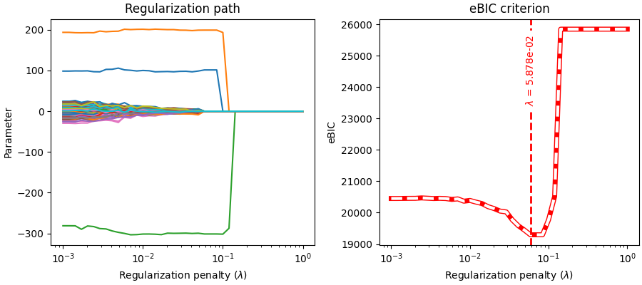
Figure 2: Regularization path, i.e. values of $\beta$, in solid line and the eBIC criterion in dotted line; the dotted vertical lines represent the chosen regularization values

Regularization Path can be plotted to visualize the evolution of the support of $\beta$ with respect to the regularization parameter $\lambda$ (e.g. figure 2). This type of graph shows that the larger the regularization parameter, the more the component of the vector $\beta$ is restricted to zero. The smaller $\lambda$ is, the more $\beta$ components are free. The eBIC criterion is minimized for a value of $\lambda$ that allows us to select the true support of $\beta$.

5 Numerical experiments

In this section, we propose to study the performance of the procedure we have just presented. The numerical study is divided into two parts. First, we present results linear mixed-effect model. The goal is to demonstrate the versatility of our method in a context beyond the one for which it was initially developed ; non-linear model that does not belong to the curved exponential family. The second part will test the robustness of our method for fitting a nonlinear mixed-effect model in different configurations. For each scenario, we generate $n_{\text{run}}$ independent data set, and each time, we fit the corresponding model using the routine described in section 3.3 and get an estimate $\hat{\theta}^{\text{MLE}}_{i}$ for each run $i\in\{1,...,n_{\text{run}}\}$. To compare the results across different scenarios, we evaluate several metrics: the Relative Root Mean Square Errors (RRMSE) to measure the estimation quality of the method and the sensitivity, specificity, and accuracy to study the selection capacity of the method. Sensitivity (Se) measures the proportion of true positives (TP) correctly identified, while Specificity (Sp) quantifies the proportion of true negatives (TN) correctly identified. Accuracy (Ac) represents the overall proportion of correctly classified instances, including both TP and TN. We abbreviated false negatives and false positives by respectively FN and FP.

$$\text{RRMSE}(\hat{\theta}^{\text{MLE}}_{k,i})=\sqrt{\frac{1}{n_{\text{run}}}\sum_{i=1}^{n_{\text{run}}}\frac{(\hat{\theta}^{\text{MLE}}_{i,k}-\theta_{k})^{2}}{\theta_{k}}}~~\text{mse}(\theta^{\text{MLE}}_{k,i})=\frac{1}{n_{\text{run}}}\sum_{i=1}^{n_{\text{run}}}(\hat{\theta}^{\text{MLE}}_{i,k}-\theta_{k})^{2}$$ (10)

$$\text{Se}=\frac{TP}{TP+FN}~~\text{Sp}=\frac{TN}{TN+FP}~~\text{Ac}=\frac{TP+TN}{P+N}$$

where $\hat{\theta}^{\text{MLE}}_{i,k}$ is $i$-th estimate of the $k$-th component of $\hat{\theta}^{\text{MLE}}_{i}$.

5.1 Simulation study in a Linear Mixed Effects Model in high dimension

In this section, we compare our method the PSPG to the R package glmmLasso (Groll and Tutz [2014]). We have used the same procedure to select the regularization parameter. We use the following linear model :

$$\left\{\begin{array}[]{rl}Y_{i,j}&=Z_{ij1}+Z_{i2}\times t_{j}+\varepsilon_{i,j}\\ Z_{ij1}&\sim\mathcal{N}(\mu_{1}+X_{i,j}\beta,\gamma_{1}^{2})\\ Z_{2}&\overset{i.i.d}{\sim}\mathcal{N}(\mu_{2},\gamma_{2}^{2})\\ \varepsilon_{i,j}&\overset{i.i.d}{\sim}\mathcal{N}(0,\sigma)\end{array}\right.$$ (11)

The model parameters are $\beta\in\mathbb{R}^{p}$, $\mu={\left(\mu_{1},\mu_{2}\right)}\in\mathbb{R}^{2}$, and $\gamma_{1},\gamma_{2},\sigma\in{\left(\mathbb{R}^{*}_{+}\right)}^{3}$. In this model, high-dimensional covariates add variability between individuals. We generated $30$ data sets independently according to equation 11 for several scenarios . It is assumed that each individual was observed at the same time $J=10$ over a range between $0$ and $1$, equally spaced. We used the following value for the parameter : $\mu={\left(2,5\right)}$, $\gamma_{1}=1,\gamma_{2}=2$ and $\sigma=1$. For each different value of $p$, we choose the vector $\beta$ such that the first three components are equal to $(\beta_{1},\beta_{2},\beta_{3})=(8,-10,20)$ and the rest are equal to zero. Additionally, we generate the matrix of covariates $X$ with $N$ rows and $p$ columns, following a uniform distribution $X_{i,k}\sim\mathcal{U}([-1,1]);~\forall i\in\{1,...,N\},\forall k\in\{1,...,p\}$.

By testing scenarios with increasing numbers of individuals $N\in\{100,100\}$, we show how our method estimates more accurately. In parallel we show different scenarios where the number of covariates increases $P\in\{200,500\}$. We then show how our method, despite the high-dimensional context, manages to select the most explanatory variables. tables 5 and 1 shows the mean value over the $30$ data sets of the Relative Root Mean Square Errors (RRMSE see 10) for each model parameter (see 11), along with their estimates. To assess the selection variable capacity of our method , we present selection scores in table 2 (the higher the better, except for mse). Whatever the configuration, our method PSPG and glmmLasso perform very similar in selecting the right covariates. However, we emphasize that PSPG adequately estimates the variances of the random effects in this model, unlike glmmLasso.

Table 1: Average Relative Root Mean Square Errors (RRMSE) and parameter estimates over 30 repetitions for the Linear Mixed Effects Model (LMEM) with $P=500$. Where $\hat{\theta}_{\textsc{PSPG}}$ and $\hat{\theta}_{\textsc{glmmLasso}}$ are the estimates using the PSPG and glmmLasso methods, respectively.

		P = 500
		N = 100				N = 200
		PSPG		glmmLasso		PSPG		glmmLasso
	$\theta^{*}$	$\hat{\theta}_{\textsc{PSPG}}$	RRMSE	$\hat{\theta}_{\textsc{glmmLasso}}$	RRMSE	$\hat{\theta}_{\textsc{PSPG}}$	RRMSE	$\hat{\theta}_{\textsc{glmmLasso}}$	RRMSE
$\mu_{1}$	2.00	1.98	6.36	1.98	6.15	1.98	3.97	2.00	3.64
$\mu_{2}$	5.00	5.03	4.03	5.03	3.69	5.01	2.70	5.01	3.49
$\gamma_{1}^{2}$	1.00	1.00	20.55	0.61	39.38	1.01	13.92	0.61	39.53
$\gamma_{2}^{2}$	4.00	3.93	17.32	0.88	78.11	4.03	12.72	0.88	77.92
$\sigma^{2}$	1.00	0.99	4.99	0.98	5.00	1.01	3.91	0.98	3.97
$\beta_{1}$	8.00	8.14	7.33	8.13	7.45	8.08	5.35	7.98	5.45
$\beta_{2}$	-10.00	-9.98	6.05	-10.00	6.63	-9.99	3.91	-9.96	4.22
$\beta_{3}$	20.00	19.98	3.30	19.97	3.42	19.98	1.91	19.97	2.14

Table 2: Average of sensitivity (Se), specificity (Sp), accuracy (Ac), mean square error (mse) over $30$ repetitions within the LMEM.

	P = 200				P = 500
	N = 100		N = 200		N = 100		N = 200
	PSPG	glmmLasso	PSPG	glmmLasso	PSPG	glmmLasso	PSPG	glmmLasso
Ac	1.000	1.000	1.000	1.000	1.000	1.000	1.000	1.000
Se	1.000	1.000	1.000	1.000	1.000	1.000	1.000	1.000
Sp	1.000	1.000	1.000	1.000	1.000	1.000	1.000	1.000
mse	4.25e-03	3.44e-03	1.96e-03	1.87e-03	1.90e-03	1.94e-03	5.99e-04	8.17e-04

5.2 Simulation study in a Non-Linear Mixed-Effects Model in high dimension

We study this section the model presented in (1), but we only position the high-dimensional variables on the logistic’s midpoint. The model can be written as follows:

$$\left\{\begin{array}[]{rl}Y_{i,j}&=\dfrac{Z_{i1}}{1+\exp{\left(-\frac{t_{ij}-Z_{i2}}{\alpha}\right)}}+\varepsilon_{i,j}\\ Z_{1}&\overset{i.i.d}{\sim}\mathcal{N}(\mu_{1}+X_{i}\beta,\gamma_{1}^{2})\\ Z_{2}&\overset{i.i.d}{\sim}\mathcal{N}(\mu_{2},\gamma_{2}^{2})\\ \varepsilon_{i,j}&\overset{i.i.d}{\sim}\mathcal{N}(0,\sigma)\end{array}\right.$$ (12)

The model parameters are $\beta\in\mathbb{R}^{p}$, $\mu={\left(\mu_{1},\mu_{2}\right)}\in\mathbb{R}^{2}$, and $\gamma_{1},\gamma_{2},\sigma\in{\left(\mathbb{R}^{*}_{+}\right)}^{3}$. $Z_{i1}$ represents the asymptotic maximum value of the curve, $Z_{i2}$ represents the value of the logistic’s midpoint, and $\alpha$ represents the logistic growth rate. This model does not belong to the curved exponential family as explain before. We chose to explain a part of the variability of the logistic’s midpoint by the high-dimensional covariates. We generated $100$ data sets independently according to equation 12 each times for several scenarios. It is assumed that each individual was observed at the same time $J=15$ over a range between $150$ and $3000$, equally spaced. We used the following value for the parameter : $\mu={\left(200,1200\right)}$, $\gamma=\operatorname{\text{diag}}(7^{2},30^{2})$, $\alpha=300$ and $\sigma^{2}=30$. For each different value of $p$, we choose the vector $\beta$ such that the first three components are equal to $(100,200,-300)$ and the rest is equal to zero. Additionally, we generate the matrix of covariates $X_{i}$ with $N$ rows and $p$ columns, following a uniform distribution $X_{i,k}\sim\mathcal{U}([-1,1]);~\forall i\in{1,...,N},\forall k\in\{1,...,p\}$.

As with the linear model, we present scenarios with an increasing number of individuals $N\in\{100,200\}$ and covariates size $p\in\{200,500,1000\}$. Tables 3 and 6 summarize the results of the estimation of the model parameters for $N=100$ and $N=200$ respectively. And table 4 summarize selection scores of the covariates. We observe that parameter estimation is accurate in all configurations. As expected, the Relative Root mean squared errors decrease with $N$ for a given covariate size $p$. For $N=100$, we observe that the relative root mean square errors increase with $p$, which can be explained by the fact that the enormous size of the covariates increases the difficulty of the selection procedure. The phenomenon is less pronounced as the sample size increases, which reflects the asymptotically expected behaviour.

Table 3: Average Relative Root Mean Square Errors (RRMSE) and parameter estimates over 100 repetitions for the Non Linear Mixed Effects Model (NLMEM) with $N=100$.

		N = 100
		P = 200		P = 500		P = 1000
	$\theta^{*}$	$\hat{\theta}$	RRMSE	$\hat{\theta}$	RRMSE	$\hat{\theta}$	RRMSE
$\mu_{1}$	200.00	200.08	0.51	199.95	0.51	199.98	0.48
$\mu_{2}$	1200.00	1200.87	0.28	1200.69	0.28	1200.47	0.30
$\gamma_{1}^{2}$	49.00	48.61	14.91	49.01	15.33	48.68	15.16
$\gamma_{2}^{2}$	900.00	847.08	19.46	832.47	20.33	967.13	98.62
$\tau$	300.00	300.24	0.58	300.03	0.65	300.23	0.64
$\sigma^{2}$	30.00	30.11	3.99	30.10	3.96	30.05	4.15
$\beta_{0}$	100.00	100.45	4.33	99.90	3.96	97.99	14.75
$\beta_{1}$	200.00	200.13	1.83	200.06	1.95	199.63	2.02
$\beta_{2}$	-300.00	-300.50	1.19	-300.40	1.34	-299.67	1.58

Table 4: Average sensitivity (Se), specificity (Sp), accuracy (Ac), and mean square error (mse) over 100 repetitions for the Non-Linear Mixed Effects Model (NLMEM)

	N = 100			N = 200
	P = 200	P = 500	P = 1000	P = 200	P = 500	P = 1000
Ac	1.000	1.000	1.000	1.000	1.000	1.000
Se	1.000	1.000	0.993	1.000	1.000	1.000
Sp	0.999	1.000	1.000	1.000	1.000	1.000
mse	2.61e-01	1.10e-01	2.72e-01	1.22e-01	4.98e-02	2.54e-02

As an illustration, figure 1 display the estimated parameter as a function of iterations during the execution of the PSPG algorithm. We can observe the convergence of the algorithm to the true parameter values used in the simulation.

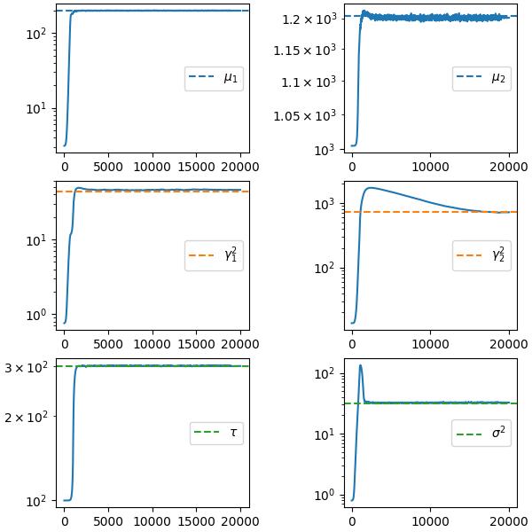
Figure 1: Parameter estimates across the PSPG iterations within the logistic NLMEM. Dotted lines : simulated value

6 Conclusion and perspectives

In this work, we jointly addressed variable selection in high dimension and parameter estimation in the nonlinear mixed-effect model that does not belong to the exponential family. To estimate the unknown parameters, we conduct a preconditioned stochastic proximal gradient to deal with the latent variables and the LASSO penalty. We use the eBIC criterion to perform an model selection procedure. Our methodology has been thoroughly evaluated in simulation study to demonstrate its performance. One interesting perspective of this work consists of studying theoretical properties of the estimator and the prediction after the model selection step.

Funding and Acknowledgements

This work was funded by the https://stat4plant.mathnum.inrae.fr/(Stat4Plant) project ANR-20-CE45-0012.

Appendix

Appendix A. Simulation study results for LMEM and NLMEM

Table 5: Average Relative Root Mean Square Errors (RRMSE) and parameter estimates over 30 repetitions for the Linear Mixed Effects Model (LMEM) with $P=200$. Where $\hat{\theta}_{\textsc{PSPG}}$ and $\hat{\theta}_{\textsc{glmmLasso}}$ are the estimates using the PSPG and glmmLasso methods, respectively.

		P = 200
		N = 100				N = 200
		PSPG		glmmLasso		PSPG		glmmLasso
	$\theta^{*}$	$\hat{\theta}_{\textsc{PSPG}}$	RRMSE	$\hat{\theta}_{\textsc{glmmLasso}}$	RRMSE	$\hat{\theta}_{\textsc{PSPG}}$	RRMSE	$\hat{\theta}_{\textsc{glmmLasso}}$	RRMSE
$\mu_{1}$	2.00	1.97	6.85	1.98	6.13	2.00	4.35	2.00	3.90
$\mu_{2}$	5.00	5.03	3.71	5.03	3.70	5.01	3.00	5.01	3.54
$\gamma_{1}^{2}$	1.00	0.99	19.59	0.61	39.74	0.99	15.24	0.61	39.24
$\gamma_{2}^{2}$	4.00	3.94	17.35	0.88	78.10	4.09	12.94	0.89	77.86
$\sigma^{2}$	1.00	0.99	5.09	0.98	5.07	0.99	3.52	0.98	4.08
$\beta_{1}$	8.00	8.04	7.22	8.05	7.20	8.05	4.40	8.03	4.61
$\beta_{2}$	-10.00	-9.98	5.49	-9.97	5.81	-10.04	3.88	-9.97	4.05
$\beta_{3}$	20.00	19.99	2.79	19.98	2.89	19.95	2.17	19.99	2.15

Table 6: Average Relative Root Mean Square Errors (RRMSE) and parameter estimates over 100 repetitions for the Non-Linear Mixed Effects Model (NLMEM) with $N=200$.

		N = 200
		P = 200		P = 500		P = 1000
	$\theta^{*}$	$\hat{\theta}$	RRMSE	$\hat{\theta}$	RRMSE	$\hat{\theta}$	RRMSE
$\mu_{1}$	200.00	200.01	0.33	199.96	0.35	199.89	0.36
$\mu_{2}$	1200.00	1199.95	0.23	1200.04	0.26	1200.07	0.24
$\gamma_{1}^{2}$	49.00	47.72	11.90	48.38	11.89	48.05	11.55
$\gamma_{2}^{2}$	900.00	903.22	12.96	904.94	14.41	902.09	13.90
$\tau$	300.00	299.63	0.46	299.84	0.45	299.86	0.42
$\sigma^{2}$	30.00	30.08	3.06	30.13	3.02	30.14	3.11
$\beta_{0}$	100.00	100.16	2.74	100.11	2.71	100.09	3.11
$\beta_{1}$	200.00	200.10	1.34	200.27	1.42	199.57	1.28
$\beta_{2}$	-300.00	-299.96	0.90	-299.67	1.02	-300.27	1.00

References

- Baey et al. [2023] Charlotte Baey, Maud Delattre, Estelle Kuhn, Jean-Benoist Leger, and Sarah Lemler. Efficient preconditioned stochastic gradient descent for estimation in latent variable models. In Proceedings of the 40th International Conference on Machine Learning, ICML’23. JMLR.org, 2023.
- Becker and Fadili [2012] Stephen Becker and Jalal Fadili. A quasi-newton proximal splitting method. In F. Pereira, C.J. Burges, L. Bottou, and K.Q. Weinberger, editors, Advances in Neural Information Processing Systems, volume 25. Curran Associates, Inc., 2012. URL https://proceedings.neurips.cc/paper_files/paper/2012/file/e034fb6b66aacc1d48f445ddfb08da98-Paper.pdf.
- Bertrand and Balding [2013] Julie Bertrand and David J Balding. Multiple single nucleotide polymorphism analysis using penalized regression in nonlinear mixed-effect pharmacokinetic models. Pharmacogenetics and genomics, 23(3):167–174, 2013.
- Bhatnagar et al. [2020] Sahir R Bhatnagar, Yi Yang, Tianyuan Lu, Erwin Schurr, JC Loredo-Osti, Marie Forest, Karim Oualkacha, and Celia MT Greenwood. Simultaneous snp selection and adjustment for population structure in high dimensional prediction models. PLoS genetics, 16(5):e1008766, 2020.
- Chen and Rockafellar [1997] George H.-G. Chen and R. Tyrrell Rockafellar. Convergence rates in forward-backward splitting. SIAM J. Optim., 7:421–444, 1997. URL https://api.semanticscholar.org/CorpusID:7104716.
- Chen and Chen [2008] Jiahua Chen and Zehua Chen. Extended bayesian information criteria for model selection with large model spaces. Biometrika, 95(3):759–771, 2008. ISSN 00063444, 14643510. URL http://www.jstor.org/stable/20441500.
- Chouzenoux et al. [2014] Emilie Chouzenoux, Jean-Christophe Pesquet, and Audrey Repetti. Variable metric forward—backward algorithm for minimizing the sum of a differentiable function and a convex function. J. Optim. Theory Appl., 162(1):107–132, July 2014. ISSN 0022-3239. doi: 10.1007/s10957-013-0465-7. URL https://doi.org/10.1007/s10957-013-0465-7.
- Davidian [2017] Marie Davidian. Nonlinear models for repeated measurement data. Routledge, 2017.
- Debavelaere and Allassonnière [2021] Vianney Debavelaere and Stéphanie Allassonnière. On the curved exponential family in the stochastic approximation expectation maximization algorithm. ESAIM: Probability & Statistics, 25, 2021.
- Delattre and Kuhn [2023] Maud Delattre and Estelle Kuhn. Computing an empirical Fisher information matrix estimate in latent variable models through stochastic approximation. Computo, 2023. ISSN 2824-7795. doi: 10.57750/r5gx-jk62. URL https://computo.sfds.asso.fr/published-202311-delattre-fim/.
- Delattre et al. [2014] Maud Delattre, Marc Lavielle, and Marie-Anne Poursat. A note on BIC in mixed-effects models. Electronic Journal of Statistics, 8(1):456 – 475, 2014. doi: 10.1214/14-EJS890. URL https://doi.org/10.1214/14-EJS890.
- Delyon et al. [1999a] Bernard Delyon, Marc Lavielle, and Eric Moulines. Convergence of a stochastic approximation version of the em algorithm. Annals of statistics, pages 94–128, 1999a.
- Delyon et al. [1999b] Bernard Delyon, Marc Lavielle, and Eric Moulines. Convergence of a stochastic approximation version of the EM algorithm. The Annals of Statistics, 27(1):94–128, 1999b. ISSN 00905364. URL http://www.jstor.org/stable/120120. Publisher: Institute of Mathematical Statistics.
- Duchi et al. [2011] John Duchi, Elad Hazan, and Yoram Singer. Adaptive subgradient methods for online learning and stochastic optimization. Journal of Machine Learning Research, 12(61):2121–2159, 2011. URL http://jmlr.org/papers/v12/duchi11a.html.
- Fort et al. [2019] Gersende Fort, Edouard Ollier, and Adeline Samson. Stochastic proximal-gradient algorithms for penalized mixed models. Statistics and Computing, 29:231–253, 2019.
- Geman and Geman [1984] Stuart Geman and Donald Geman. Stochastic relaxation, gibbs distributions, and the bayesian restoration of images. IEEE Transactions on Pattern Analysis and Machine Intelligence, PAMI-6(6):721–741, 1984. ISSN 0162-8828. doi: 10.1109/TPAMI.1984.4767596. URL http://ieeexplore.ieee.org/document/4767596/.
- Groll and Tutz [2014] Andreas Groll and Gerhard Tutz. Variable selection for generalized linear mixed models by l1-penalized estimation. Statistics and Computing, 24(2):137–154, 2014. ISSN 1573-1375. doi: 10.1007/s11222-012-9359-z. URL https://doi.org/10.1007/s11222-012-9359-z.
- Heuclin et al. [2020] Benjamin Heuclin, Frédéric Mortier, Catherine Trottier, and Marie Denis. Bayesian varying coefficient model with selection: An application to functional mapping. Journal of the Royal Statistical Society: Series C (Applied Statistics), 70, 11 2020. doi: 10.1111/rssc.12447.
- Jürg Schelldorfer and Bühlmann [2014] Lukas Meier Jürg Schelldorfer and Peter Bühlmann. Glmmlasso: An algorithm for high-dimensional generalized linear mixed models using l1-penalization. Journal of Computational and Graphical Statistics, 23(2):460–477, 2014. doi: 10.1080/10618600.2013.773239. URL https://doi.org/10.1080/10618600.2013.773239.
- Kingma and Ba [2017] Diederik P. Kingma and Jimmy Ba. Adam: A method for stochastic optimization, 2017. URL https://arxiv.org/abs/1412.6980.
- Leger [2023] Jean-Benoist Leger. Parametrization cookbook: A set of bijective parametrizations for using machine learning methods in statistical inference. arXiv preprint arXiv:2301.08297, 2023.
- Moreau [1962] Jean Jacques Moreau. Fonctions convexes duales et points proximaux dans un espace hilbertien. Comptes rendus hebdomadaires des séances de l’Académie des sciences, 255:2897–2899, 1962.
- Naveau et al. [2024] Marion Naveau, Guillaume Kon Kam King, Renaud Rincent, Laure Sansonnet, and Maud Delattre. Bayesian high-dimensional covariate selection in non-linear mixed-effects models using the saem algorithm. Statistics and Computing, 34(1):53, 2024.
- Ng et al. [2012] Shu Kay Ng, Thriyambakam Krishnan, and Geoffrey J McLachlan. The em algorithm. Handbook of computational statistics: concepts and methods, pages 139–172, 2012.
- Ollier [2022] Edouard Ollier. Fast selection of nonlinear mixed effect models using penalized likelihood. Computational Statistics & Data Analysis, 167:107373, 2022.
- Pinheiro and Bates [2006] José Pinheiro and Douglas Bates. Mixed-effects models in S and S-PLUS. Springer science & business media, 2006.
- Rockafellar [1976] R. Tyrrell Rockafellar. Monotone operators and the proximal point algorithm. SIAM Journal on Control and Optimization, 14(5):877–898, 1976. ISSN 0363-0129, 1095-7138. doi: 10.1137/0314056. URL http://epubs.siam.org/doi/10.1137/0314056.
- Schelldorfer et al. [2014] Jürg Schelldorfer, Lukas Meier, and Peter Bühlmann. Glmmlasso: an algorithm for high-dimensional generalized linear mixed models using -penalization. Journal of Computational and Graphical Statistics, 23(2):460–477, 2014.
- Schwarz [1978] Gideon Schwarz. Estimating the dimension of a model. The Annals of Statistics, 6(2):461–464, 1978. ISSN 00905364. URL http://www.jstor.org/stable/2958889. Publisher: Institute of Mathematical Statistics.
- Tibshirani [1996] Robert Tibshirani. Regression shrinkage and selection via the lasso. Journal of the Royal Statistical Society: Series B (Methodological), 58(1):267–288, 1996. ISSN 00359246. doi: 10.1111/j.2517-6161.1996.tb02080.x. URL https://onlinelibrary.wiley.com/doi/10.1111/j.2517-6161.1996.tb02080.x.
- Tieleman [2012] T. Tieleman. Lecture 6.5‐rmsprop: Divide the gradient by a running average of its recent magnitude, 2012. URL https://cir.nii.ac.jp/crid/1370017282431050757.
- Tseng [2000] P. Tseng. A modified forward-backward splitting method for maximal monotone mapping. Siam Journal on Control and Optimization - SIAM, 38, 01 2000.