Study of Multi-Wavelength Variability, Emission Mechanism and Quasi-Periodic Oscillation for Transition Blazar S5 1803+784

Abstract

This work present the results of a multi-epoch observational study of the blazar S5 1803+784, carried out from 2019 to 2023. The analysis is based on simultaneous data obtained from the Swift/UVOT/XRT, ASAS-SN, and Fermi-LAT instruments. A historically high $\gamma$-ray flux observed for this source on march 2022 ($\mathrm{2.26\pm 0.062)\times 10^{-6}~phcm^{-2}s^{-1}}$. This study investigates the $\gamma$-ray emission from a blazar, revealing a dynamic light curve with four distinct flux states: quiescent and high-flux by using the Bayesian Blocks (BB) algorithm. A potential transient quasi-periodic signal with an oscillation timescale of $\sim$411 days was identified, showing a local significance level surpassing 99.7$\%$ from the Lomb-Scargle Periodogram (LSP) and Damped Random Walk (DRW) analysis and exceeds 99.5$\%$ from the Weighted Wavelet Z-Transform (WWZ) analysis. The observed QPO was confirmed through an autoregressive process (AR(1)), with a significance level exceeding 99$\%$, suggesting a potential physical mechanism for such oscillations involves a helical motion of a magnetic plasma blob within the relativistic jet. Log parabola modeling of the $\gamma$-ray spectrum revealed a photon index ($\alpha_{\gamma}$) variation of 1.65$\pm$0.41 to 2.48$\pm$0.09 with a steepening slope, potentially indicative of particle cooling, changes in radiative processes, or modifications in the physical parameters. The $\alpha_{\gamma}$ of 2.48$\pm$0.09 may hint at an evolutionary transition state from BL Lac to FSRQ. A comparative analysis of variability across different energy bands reveals that Optical/UV and GeV emissions display greater variability compared to X-rays. Broadband SED modeling shows that within a one-zone leptonic framework, the SSC model accurately reproduces flux states without external Compton contributions, highlighting magnetic fields crucial role.

[first]Department of Physics,, University of Kashmir,, city=Srinagar, postcode=190006, state=Kashmir, country=India

[second]S N Bose National Centre for Basic Sciences,,addressline=Block JD, Salt Lake, city=Kolkata, postcode=700106, state=West Bengal, country=India

[third]Department of Physics, Central University of Kashmir,, addressline=Ganderbal, postcode=191131, state=Kashmir, country=India

1 Introduction

Blazars are a peculiar class of radio-loud AGNs, distinguished by relativistic jets that are closely aligned with the observer’s line of sight Urry and Padovani (1995). The relativistic jets in the blazar are efficient particle accelerators and emit non-thermal radiation across the electromagnetic spectrum. This non-thermal emission from the relativistic jets dominates the entire broadband spectra Dondi and Ghisellini (1995); Urry and Padovani (1995). Strong $\gamma-$ray emissions, a high degree of polarization, and frequent variability in flux and spectra are some other characteristics of blazars Wills et al. (1992); Ackermann and et al. (2015); Fan et al. (2018); Ajello et al. (2020); Zhang et al. (2021).

The broadband spectral energy distribution (SED) of blazars shows a two-humped structure, with the low-energy component (peaking in the submillimeter to soft X-ray range) attributed to synchrotron radiation from relativistic electrons in the jet, while the high-energy component (peaking at MeV to TeV energies) is explained by using either the leptonic model or hadronic model Abdo et al. (2010a). According to the leptonic model, the high-energy component is attributed to the inverse Compton scattering of low-energy photons. This can involve low-energy synchrotron photons within the jet, known as the synchrotron self-Compton (SSC) process, or photons originating from external sources outside the jet (such as from the accretion disk, broad line region (BLR) and Dusty Torus), referred to as the external Compton process Finke (2013); Bloom and Marscher (1996); Dermer and Schlickeiser (2002); Dermer et al. (2009). Alternatively, hadronic models could also explain the high energy emission in blazars. The high energy peak may be the consequence of secondary decay products of charged particles, primarily pions, or synchrotron radiation from protons Böttcher et al. (2013).

Blazars are often classified as BL Lacertae objects (BL Lacs), and flat-spectrum radio quasars (FSRQs) based on their spectral properties. In their optical spectrum, FSRQs show strong emission line characteristics, while BL Lacs have weak or no emission line features (Urry and Padovani, 1995). Based on the peak frequency of the synchrotron component, blazars are also classified into low synchrotron peak (LSP; $\nu_{p}<10^{14}$ Hz), intermediate-synchrotron peaked (ISP; $10^{14}<\nu_{p}<10^{15}$) and high synchrotron peaked (HSP; $\nu_{p}>10^{15}$) blazars (Padovani and Giommi, 1995). The FSRQs belong to the LSP category, while a large fraction of BL Lacs are HSP sources (Rajput et al., 2020). Additionally, blazars that exhibit properties of both FSRQs and BL Lacs in varying flux states are known as transition blazars/changing look blazars (CLB) (Ghisellini et al., 2013; Mishra et al., 2021; Xiao et al., 2022; Pandey et al., 2024; Ren et al., 2024). The shifting poses significant challenges to the AGN unification model (Mishra et al., 2021; Peña-Herazo et al., 2021). A promising explanation for this transition is a sudden change in accretion ratio.

Blazars exhibit stochastic flux variability across multiple wavelengths, with timescales ranging from minutes to years. However, some blazars exhibit persistent or transient quasi-periodic variability Sobolewska et al. (2014); Gierliński et al. (2008); Abdo et al. (2010b); King et al. (2013); Alston et al. (2014); Ackermann et al. (2015a); Peñil et al. (2022); Ren et al. (2023); Sharma et al. (2024a). The $\gamma$-ray emission in blazars is believed to originate from their relativistic jets, making the investigation of quasi-periodic signals in this band crucial for understanding jet physics and particle acceleration mechanisms. The continuous sky monitoring by Fermi’s Large Area Telescope (LAT) provides an excellent opportunity to explore such features in $\gamma$-rays using long-term temporal observations. Notably, the blazar PG 1553+113 was the first $\gamma$-ray source reported to exhibit a quasi-periodic oscillation (QPO) with a period of 2.18$\pm$0.08 years, completing three full cycles Ackermann et al. (2015a). It is believed that the blazer is in a binary system, thus a persistent QPO source Tavani et al. (2018). Since its discovery, this source has become an ideal candidate for continuous monitoring in $\gamma$-rays and across other wavelengths. Numerous transient and persistent quasi-periodic oscillations (QPOs) have been reported in the $\gamma$-ray emission of blazars, with oscillation timescales ranging from days to years Zhou et al. (2018); Benkhali et al. (2020); Sarkar et al. (2020, 2021); Peñil et al. (2022); Das et al. (2023); Banerjee et al. (2023); Prince et al. (2023); Li et al. (2023); Sharma et al. (2024a). Peñil et al. (2022) analyzed a sample of 24 blazars using approximately 12 years of Fermi-LAT observations, identifying five sources with persistent periodic behavior at high significance levels. Zhou et al. (2018) were the first to report a significant transient QPO in a blazar, with a period of $\sim$34.5 days and a significance exceeding 4.6$\sigma$. More recently, Ren et al. (2023) conducted a QPO study on a sample of 35 AGNs observed in $\gamma$-rays and identified a transient QPO with a period of $\sim$39 days in the source B2 1520+31, persisting for 17 complete cycles. Additionally, several studies have documented both transient and persistent multi-wavelength QPOs in blazars. A widely considered physical explanation for these $\gamma$-ray QPOs involves the helical jet model, where the periodic variation in the viewing angle of the emission region modulates the observed flux. However, the precise physical mechanisms driving this behavior remain elusive.

Blazar S5 1803+78 is a BL Lac type identified by Biermann et al. (1981). The redshift of this blazar is z = 0.684, determined by Lawrence et al. (1996) and confirmed by Rector and Stocke (2001) . The source has been identified as LSP in the AGN unification scheme (Urry and Padovani (1995)). Initially, the source was extensively used for geodynamics studies Gabuzda (1999); Gabuzda et al. (2000). Later, optical and radio study of this source was carried out by Nesci et al. (2002, 2012) during the optical active state of the source. During that period, the radio (8.4 GHz) light curves showed modest fluctuations lacking periodic signatures. Interestingly, Kun et al. (2018) investigated the relativistic jet dynamics using 30 VLBI observations, revealing a significant 6-year periodicity. However, previous long-term optical observations showed no evidence of periodicity Nesci et al. (2002, 2012). Recently, Butuzova et al. (2025) studied the variability evolution of this source using TESS observations, finding that its variability timescales span from several hours to days. The authors suggested that such a pattern of variability can be attributed to contributions from different regions within the emission zone. Alternatively, it may also be explained by the continuous formation and evolution of sub-components in the emitting region, each with varying sizes and Doppler factors. Another study on this source examined morphological changes in its radio structure following the $\gamma$-ray flares, during the period between MJD 59063.5 – 59120.5, and reported the emergence of two new components from the core propagated outwards Nesci et al. (2021). The broadband spectra of the source during intense flaring episodes were modeled using a single-zone leptonic framework that incorporated external Compton scattering from a dusty torus, providing constraints on the underlying physical parameters Omojola and Chen (2021). Furthermore, a multi-wavelength study spanning MJD 58727 – 59419, utilizing data from Fermi-LAT, SWIFT/XRT/UVOT, NuSTAR, and TUBITAK observations, explored the source’s high-flux state. Although simultaneous optical and X-ray data were unavailable, the study revealed that blazar flares exhibit day-scale variability with similar rise and decay timescales, indicating a compact emission region near the central engine Priya et al. (2022). Notably, a bright optical flare was observed between May 2020 and May 2021, however, the optical variability during this period was less pronounced compared to the non-flaring state Agarwal et al. (2022).
Our study presents a comprehensive analysis of the blazar S5 1803+784, utilizing simultaneous observations from Swift/XRT/UVOT, ASAS-SN, and Fermi-LAT. We investigate the source’s temporal behavior, identifying variability patterns and spectral changes in $\gamma$-ray emission that provide insights into the underlying physical processes. Additionally, we also search for a transient quasi-periodic oscillation in a 10-day binned $\gamma$-ray light curve. By employing the one-zone leptonic model, we fitted the broadband spectrum in different flux states and constrained the underlying physical parameters in different flux states. This work is structured in the following ways: §1 introduction of the Source. Section §2 details observations and data processing techniques. In section §3, we report the multi-wavelength temporal and spectral results of S5 1803+784 using Swift/UVOT/XRT, ASAS-SN, and Fermi-Lat data. Finally, the paper concludes with a summary and discussion in Section §4.

2 Observations and Data reduction

2.1 Swift-XRT

Swift is a multi-wavelength space-based observatory equipped with Burst Alert Telescope (BAT), X-ray Telescope (XRT), and Ultraviolet/Optical Telescope (UVOT) (Burrows et al., 2005). Covering a broad spectrum of electromagnetic radiation, the Swift observes the sky across multiple wavebands, including Optical, Ultraviolet, soft, and hard X-rays. The Swift XRT is sensitive to soft X-rays in the energy range of 0.3 – 10 keV, it helps in measuring the fluxes, light curves, and spectra of the source. Swift conducted a total of 43 observations of the source S5 1803+784, these observations include both the quiescent and flaring states. Using “xrtpipeline” Version: 0.13.5, and the calibration file (CALDB, version: 20190910), we created the cleaned event files for the photon counting (PC) mode of the data. The “xselect” (v2.5b) tool was used to extract the source and background spectrum files. A circular region with a radius of 25 pixels was centered on the source location to define the source region, while a background region was selected as a circular area offset by 50 pixels from the source. To create the required auxiliary response file (ARF), “xrtmkarf” tool was used. The “grppha” task was applied to ensure the validity of the spectrum for $\chi^{2}$ statistics. This involved binning the spectrum to ensure a minimum of 20 counts per bin. The HEASOFT package ”XSPEC” (v12.13.0c) (Arnaud, 1996) was used to perform X-ray spectra analysis in the energy range 0.3 – 10.0  keV. The X-ray spectra were fitted with a Tbabs $\times$ power law (PL)/broken power law (BPL)/log parabola model. However, power law and log parabola provide a better fit during the X-ray spectral fit. During the spectral fitting, the neutral hydrogen column density for this source was fixed at $N_{H}=3.64\times 10^{20},\text{cm}^{-2}$ (Murphy et al., 1996), while other parameters of the model were allowed to vary freely.

2.2 Swift-UVOT

Swift-UVOT offers Optical/UV data through six filters U (3465 Å), V (5468 Å), B (4392 Å), UVW1 (2600 Å), UVM2 (2246 Å), and UVW2 (1928 Å) (Roming et al., 2005). Swift-UVOT telescope (Roming et al., 2005) has also observed the BL Lac source S5 1803+784 simultaneously with the Swift-XRT. The Swift-UVOT data for the source covers all six filters during epoch S4 but exhibits limited filter availability during epochs S1 (U, UVW1, UVW2), S2 (UVW1, UVM2), and S3 (U, UVW1, UVW2, UVM2). We obtained data of S5 1803+784 from the HEASARC Archive and utilized HEASoft (v6.26.1) to process it into a usable scientific format. The UVOTSOURCE package included in HEASoft (v6.26.1) was used for image processing, while the UVOTIMSUM package combined multiple images across filters. Photometry adhered to the procedures outlined by Poole et al. (2008), with a circular source region of 5 arcsecs centered at the source location and a background region two times larger than the source region. The uvotsource tool was utilized to obtain the magnitude, which was then adjusted for reddening and galactic extinction using a $E(B-V)$ value of 0.0448 Schlafly and Finkbeiner (2011). Subsequently, these corrected magnitudes were converted into flux values using the zero point magnitudes specific to Swift-UVOT, as described by Giommi et al. (2006).

2.3 Fermi-LAT

Fermi-LAT serves as one of the two instruments onboard Fermi $\gamma$-ray space telescope, featuring a wide field of view of approximately 2.4 Sr (Atwood et al., 2009). It has functioned as a pair conversion telescope in near-Earth orbit since June 2008, capable of detecting high-energy $\gamma$-rays within the energy range of 20 MeV to 1 TeV Atwood et al. (2009). Functioning in all-sky scanning mode, it systematically scans the entire sky every three hours, enabling the identification of numerous $\gamma$-ray sources. One of the sources that Fermi-LAT frequently monitored is S5 1803+784 and has been continuously observed since August 4, 2008, at 15:43:36 UTC. Using Fermitools version 2.2.0, the data was processed following the standard analysis specified in the Fermi-LAT documentation Wood et al. (2017). A circular region of radius $15^{\circ}$ centered on the source location (RA: 270.173, Dec: 78.467) was used to extract events. Following the recommendations in the Fermitools document, the data were filtered using “evclass = 128” and “evtype = 3”. In the analysis, we have used the most recent instrument response function (IRF), “P8R3 SOURCE V3”. In order to reduce contamination from $\gamma$-rays originating from the Earth limb, a zenith angle cut greater than $90^{\circ}$ is applied. Two models were used to produce XML files: the isotropic background model “$\rm iso_{-}P8R3_{-}SOURCE_{-}V3_{-}v1.txt$” and the galactic diffusion model “$\rm gll_{-}iem_{-}v07.fits$10”.

We adopted criteria to filter out the sources with low Test Statistics (TS) i.e. below TS = 9 and generated a 10-day binned $\gamma$-ray light curve of the source of interest with TS$\>(\geq 9)$. In this process, parameters for sources positioned beyond 15^∘ from the center of ROI were fixed, while for $\leq 15^{\circ}$ were left free and were allowed to vary freely. In this project, We used the FERMIPY package to generate the 10-day binned $\gamma$-ray light curve.

2.4 ASAS-SN

All-Sky Automated Survey for Supernovae (ASAS-SN; Shappee et al. (2014); Kochanek et al. (2017) is a global network of 24 telescopes that has been monitoring the extragalactic sky since 2012. With a limiting magnitude of $\sim$17.5-18.5 in the g-band and $\sim$16.5-17.5 in the V-band depending on lunation, ASAS-SN provides valuable observations across the entire sky. For this study, we utilized g-band data, Figure 1 collected through the ASAS-SN Sky Patrol (V2.0; Shappee et al. (2014); Hart et al. (2023).

3 Multi-wavelength Temporal and Spectral results

To investigate the temporal behavior of LSP blazar S5 1803+784, Swift-XRT/UVOT observed 43 observations between MJD 58748 – 60152 along with Fermi-LAT . The X-ray and optical/UV data were analyzed using the methods outlined in §2. Figure 1 displays the resulting multi-wavelength light curves, including 10-day binned $\gamma$-ray observations in the top panel of Figure 1 along with the Bayesian Blocks. The X-ray, optical, and UV data are given in the second, third, and fourth panels from the top, respectively. The bottom panel of Figure 1 presents the ASAS-SN simultaneous observations.

The identification of flare events in the $\gamma$-ray light curve lacks a universally accepted method. However, the Bayesian Blocks (BB) algorithm has gained some popularity for detecting flares in AGN light curves. In this study, we employed the Bayesian Blocks (BB) algorithm of the Astropy package, setting the false-alarm probability to $p_{0}=0.05$, Figure 1. While applying the BB algorithm, we excluded upper limits from the $\gamma$-ray light curve analysis, as the algorithm is well-suited for handling non-uniform light curves. To estimate the flaring temporal regions, we utilized the HOP algorithm, defining a flare as any event satisfying the condition $F_{\text{BB}}>3\times\overline{F}$, where $\overline{F}=1.152\times 10^{-7}ph\ cm^{-2}\ s^{-1}$. Accordingly, we identified four epochs having simultaneous multi-wavelength observations, in which epoch S1 represents a low flux state and epochs S2, S3, and S4 represent three flaring states, see the Figure 1.

The average $\gamma$-ray flux was $6.05\times 10^{-08}ph\ cm^{-2}\ s^{-1}$ during 58819 – 58928 (S1). A high-flux state (S2) occurred during MJD 58928 – 58974, characterized by an increased average $\gamma$-ray flux of $4.40\times 10^{-07}ph\ cm^{-2}\ s^{-1}$ . Similarly, a flux state (S3) occurred during MJD 59645 - 59695, with average $\gamma$-ray flux of $6.78\times 10^{-07}ph\ cm^{-2}\ s^{-1}$. This was followed by another state (S4), identified during MJD 60100 – 60150, with an average $\gamma$-ray flux of $4.19\times 10^{-07}ph\ cm^{-2}\ s^{-1}$. A comprehensive multi-wavelength analysis of an LSP blazar was conducted, covering four epochs (S1, S2, S3, S4) and multiple energy bands. The study revealed complex variability patterns across the four epochs, with each epoch displaying distinct behaviors in three energy bands. Specifically, epoch S1 showed consistently low flux levels, while epoch S2 displayed high flux levels across all bands. In contrast, epoch S3 exhibited high $\gamma$-ray and X-ray flux, but low UVOT flux, and epoch S4 was characterized by the elevated flux in UVOT, X-ray, and $\gamma$-ray bands, offers clues to understanding the elusive nature of orphan blazars.

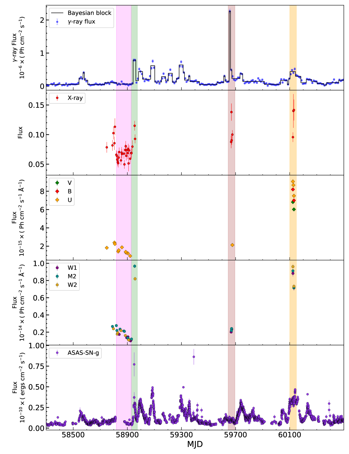
Figure 1: Multi-wavelength light curve (MWLC) obtained from ASAS-SN, Swift-XRT/UVOT, and Fermi-LAT. The top panel displays a 10-day binned $\gamma$-ray light curve (blue) obtained in the energy range of 100 MeV to 300 GeV along with the Bayesian Block (black). The top second is the light curve of X-ray data using Swift/XRT. The third and fourth panels depict Optical/UV light curves, where each point corresponds to a single observation ID. The last panel represents the ASAS-SN g-band light curve. The shaded regions in pink, green, brown, and orange throughout all five panels represent the S1, S2, S3, and S4 selected observation epochs, respectively.

3.1 Fractional Variability

To comprehensively study the statistical variability characteristic of the blazar S5 1803+784, we utilized the simultaneous multi-wavelength observations from Fermi-LAT, Swift-XRT/UVOT, and ASAS-SN, following the approach described in Edelson et al. (2002); Vaughan et al. (2003).

To measure the variability in a given sample of $\mathcal{N}$ data points $x_{i}$, the variance $\mathcal{S}^{2}$ is used, defined as:

$$\mathcal{S}^{2}=\frac{1}{\mathcal{N}-1}\sum_{i=1}^{\mathcal{N}}(\langle x\rangle-x_{i})^{2}$$ (1)

In the case of blazars, the light curve is the sample, which consists of measurement uncertainties $\sigma_{\text{err},i}$. The fractional variability tool is considered to account for these uncertainties. It incorporates the variance of the data points and the cumulative variance that is created from these measurement uncertainties. This is commonly called fractional variance excess or normalized excess variance, given by Edelson et al. (2002). To measure the variability of a source in different energy bands, the fractional variability amplitude expression has been used and is given by Vaughan et al. (2003):

$$F_{\text{var}}=\sqrt{\frac{S^{2}-\overline{\sigma_{\text{err}}^{2}}}{\overline{F}^{2}}}$$ (2)

where $S^{2}$ is the variance, $\overline{F}$ is the mean, and $\overline{\sigma_{\text{err}}^{2}}$ is the mean square of the measurement error on the flux points. The uncertainty on $F_{\text{var}}$ is given by Vaughan et al. (2003):

$$F_{\text{var,err}}=\sqrt{\frac{1}{2N}\left(\frac{\overline{\sigma_{\text{err}}^{2}}}{F_{\text{var}}\overline{F}^{2}}\right)^{2}+\frac{1}{N}\frac{\overline{\sigma_{\text{err}}^{2}}}{\overline{F}^{2}}}$$ (3)

Here, N represents the number of flux points in the light curve.

For the $\gamma$-ray, swift X-ray, swift-Optical/UV, and ASAS-SN light curves, the values of $F_{\text{var}}$ and their uncertainties are shown in Table 6. Figure 2 shows the relation between $F_{\text{var}}$ and frequency. The X-ray band has a lower variability amplitude value when compared to the values seen in the $\gamma$-ray, optical, and UV bands. Remarkably, it represents a distinct pattern to what we have observed in the BL Lac class of earlier sources such as Mrk 501 and Mrk 421 i.e., higher in X-rays compared to $\gamma$-rays Schleicher et al. (2019); Abe et al. (2023, 2024); Tantry et al. (2024). The $F_{var}$ displays a double-peak structure with higher variability at UV/Optical and $\gamma$-ray from the 4-year data set. Previous studies by Rajput et al. (2020) utilized $\gamma$-ray Space Telescope data to analyze monthly $\gamma$-ray flux variability in blazars; the dataset comprises 1120 blazars, including 481 FSRQs and 639 BL Lacs. Mean $F_{var}$ of 0.55 ± 0.33 for FSRQs, while for LSP blazars mean $F_{var}$ value of 0.54 ± 0.32. Furthermore, we quantify the variability of the $\gamma$-ray light curve by comparing the fractional amplitude values between low and high flux states, using $\sim$15 yr long lightcurve with the binning of 3-day and 7-day, as illustrated in Figure11.

Table 1: Fractional variability amplitude $F_{var}$ obtained in different energy bands. Columns 1: energy band 2: fractional variability amplitude with uncertainty.

Data set (2019–2023)
Energy band	$\rm F_{var}$
Fermi $\gamma$-ray (0.1 – 300 GeV)	1.15$\pm$0.01
Swift X-ray (0.3–10 keV)	0.27$\pm$0.02
Swift UVOT-W2	0.88$\pm$0.01
Swift UVOT-M2	0.83$\pm$0.009
Swift UVOT-W1	0.96$\pm$0.01
Swift UVOT-U	0.93 $\pm$ 0.01
ASAS-SN g-band	0.60$\pm$0.001

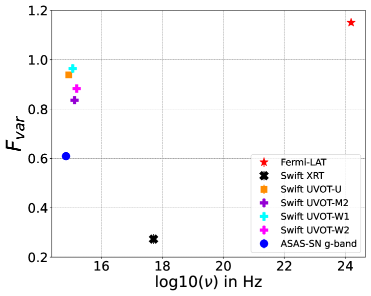
Figure 2: Fractional variability amplitude obtained in different energy bands is plotted against the frequency

3.2 Transient quasi-periodic oscillation

To investigate the presence of a transient Quasi-Periodic Oscillation (QPO) in the gamma-ray emission of the blazar S5 1803+784, we employed several analytical approaches, including the Lomb-Scargle periodogram (LSP), the Weighted Wavelet Z-transform (WWZ), a first-order autoregressive AR(1) process, the Date-Compensated Discrete Fourier Transform (DCDFT), and Damped Random Walk (DRW). Below, we provide a detailed description of these methods and the results obtained from the analysis.

3.2.1 Lomb-Scargle Periodogram

The Lomb-Scargle periodogram is a widely used and popular technique for detecting periodic signals in time series data with unevenly spaced observations Lomb (1976); Scargle (1982). It is particularly well-suited for analyzing non-uniformly sampled light curves to identify potential periodicities. In our study, we utilized the LOMB-SCARGLE class from the ASTROPY library to perform the analysis. Additionally, the uncertainties associated with the flux measurements were incorporated into the analysis. The periodogram function of the Lomb-Scargle method is defined as VanderPlas (2018)

$$\begin{split}P_{LS}(f)=\frac{1}{2}\bigg{[}&\frac{\left(\sum_{i=1}^{N}x_{i}\cos(2\pi f(t_{i}-\tau))\right)^{2}}{\sum_{i=1}^{N}\cos^{2}(2\pi f(t_{i}-\tau))}\\ &+\frac{\left(\sum_{i=1}^{N}x_{i}\sin(2\pi f(t_{i}-\tau))\right)^{2}}{\sum_{i=1}^{N}\sin^{2}(2\pi f(t_{i}-\tau))}\bigg{]}\end{split}$$ (4)

where, $\tau$ is

$$\tau=\rm{tan^{-1}}\left(\frac{\sum_{i=1}^{N}sin\left(2\pi f(t_{i}-\tau)\right)}{2(2\pi f)\sum_{i=1}^{N}cos\left(2\pi f(t_{i}-\tau)\right)}\right)$$ (5)

In our analysis, we selected the minimum ($f_{min}$ and maximum ($f_{max}$) temporal frequencies as 1/T and 1/2$\Delta T$, respectively. Here, T represents the total observation duration, and $\Delta T$ denotes the binning interval of the light curve or the time difference between consecutive data points. These parameters are critical for the Lomb-Scargle periodogram (LSP) analysis. The analysis identified a potential peak corresponding to a frequency of $0.00243\pm 0.00045\ day^{-1}$ ($\sim$411 days). The uncertainty in the detected period was estimated by fitting a Gaussian function to the periodogram peak, with the half-width at half-maximum (HWHM) of the Gaussian taken as the error on the observed period VanderPlas (2018); Sharma et al. (2024a).

3.2.2 Weighted Wavelet Z-Transform

In addition, Wavelet analysis is a robust technique for detecting periodic signals in time series by simultaneously decomposing them into frequency and time domains. This method is particularly effective for studying the evolution of QPO features, as it provides detailed insights into how potential periodic signals emerge, evolve, and fade over time Foster (1996).

In wavelet analysis, we used the abbreviated Morlet kernel, which has the following functional form:

$$f[\omega(t-\tau)]=\exp[i\omega(t-\tau)-c\omega^{2}(t-\tau)^{2}]$$ (6)

and the corresponding WWZ map is given by,

$$W[\omega,\tau:x(t)]=\omega^{1/2}\int x(t)f^{*}[\omega(t-\tau)]dt$$ (7)

Here, $f^{*}$ is the complex conjugate of the wavelet kernel f, $\omega$ is the frequency, and $\tau$ is the time-shift. For more details, see Sharma et al. (2024a), and references therein. In this study, we employed the publicly available Python WWZ code to search for periodicities. The resulting WWZ map revealed a distinct concentration of power around a frequency $0.00251\pm 0.0002\ day^{-1}$ ($\sim$ 399 days). The uncertainty on the observed period was estimated by fitting the Gaussian function to the observed prominent peak in the average WWZ.

3.2.3 First order Autoregressive process (REDFIT)

AGN light curves are generally dominated by red noise, which arises from stochastic processes in the accretion disc or jet. The emissions from blazars are well modeled using the simplest autoregressive (AR) processes, known as a first-order autoregressive (AR(I)) process Schulz and Mudelsee (2002), where the emission at an instance is related to past activities, defined as, $r(t_{i})=A_{i}r(t_{i-1})+\epsilon(t_{i})$, where the current emission ($r_{t}$) depends linearly on the previous emission ($r_{t-1}$), $A_{i}=exp\left(-(t_{i}-t_{i-1})/\tau\right)\in[0,1]$, A is the average autoregressive coefficient calculated from the mean of the sampling intervals, $\tau$ is the timescale of autoregressive process, and a random error ($\epsilon_{t}$). The power spectrum of an AR(I) process is defined as:

$$G_{rr}(f_{i})=G_{0}\frac{1-A^{2}}{1-2Acos\left(\frac{\pi f_{i}}{f_{Nyq}}\right)+A^{2}}$$ (8)

where $G_{0}$ is the average spectral amplitude, $f_{i}$ are the frequencies, and $f_{Nqy}$ is the Nyquist frequency. In this study, we used the publicly available r programming code REDFIT to estimate the red noise-corrected power spectrum. We calculated the significance of the powers in the power spectrum using equation (6). The obtained power spectrum clearly shows a significant peak at frequency $0.00237\pm 0.00049\ day^{-1}$ ($\sim 421\ days$), exceeding 99$\%$ significance level. The uncertainty value in the dominant peak frequency is HWHM from the fitting of Gaussian to the peak profile in the REDFIT power spectrum.

3.2.4 Date-compensated Discrete Fourier Transform

In this study, we also utilized the date-compensated discrete Fourier transform (DCDFT) (Ferraz-Mello, 1981; Foster, 1995; Fan et al., 2007), a Fourier-based technique. To identify periodic signatures in an unevenly sampled time series, we applied a least-squares regression using three trial functions: $\phi_{1}$(t)=1, $\phi_{2}$(t)=cos($\omega$t), and $\phi_{3}$(t)=sin($\omega$t).

The observations x(t_i) are defined as data vector

$$\ket{x}=\left[x(t_{1}),x(t_{2}),...,x(t_{N})\right]$$ (9)

To project the data onto the subspace spanned by the three trial functions defined above, we construct a set of trial vectors based on these functions, which is given as

$$\ket{\phi_{\alpha}}=\left[\phi_{\alpha}(t_{1}),\phi_{\alpha}(t_{2}),...,\phi_{\alpha}(t_{N})\right]$$ (10)

where, $\alpha$=1,2,3. The projection of $\ket{x}$ onto the subspace spanned by $\ket{\phi_{\alpha}}$ yields a model vector $\ket{y}$ and a residual vector $\ket{\Theta}$,

$$\ket{x}=\ket{y}+\ket{\Theta}$$ (11)

here, the model vector is defined as

$$\ket{y}=\sum_{\alpha}c_{\alpha}\ket{\phi_{\alpha}},$$ (12)

while the residual vector is orthogonal to the subspace,

$$\langle\phi_{\alpha}|\Theta\rangle=0,\ \ \rm{for}\ \ \rm{all}\ \ \alpha$$ (13)

now, taking the inner product of the trial vector with data vector, we can obtain coefficient $c_{\alpha}$,

$$\langle\phi_{\alpha}|x\rangle=\sum_{\beta}c_{\beta}\langle\phi_{\alpha}|\phi_{\beta}\rangle=\sum_{\beta}S_{\alpha\beta}c_{\beta}$$ (14)

where, $S_{\alpha\beta}$ defines the metric tensor for the trial subspace. The coefficient $c_{\alpha}$ can be obtained by multiplying $S_{\alpha\beta}^{-1}$ in both sides in equation 14

$$c_{\alpha}=\sum_{\beta}S_{\alpha\beta}^{-1}\langle\phi_{\beta}|x\rangle$$ (15)

Finally, the power level of DCDFT is defined as

$$P_{X}(\omega)=\frac{1}{2}N\left[\langle y|y\rangle-\langle 1|y\rangle^{2}\right]/s^{2}$$ (16)

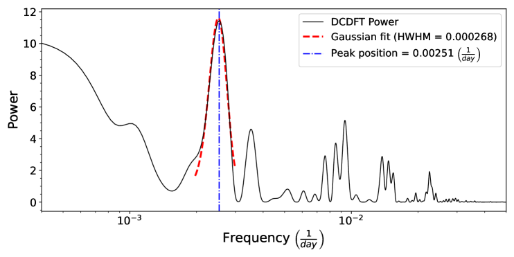
Figure 6: The date-compensated discrete Fourier transform (DCDFT) power level of $\gamma$-ray light curve of S5 1803+784 is presented here. This figure highlights the dominant peak (black) at 0.00251$\pm$0.000268 $\rm{day^{-1}}$ (blue vertical line). To estimate the uncertainty on the period, the peak is fitted with a Gaussian function (dashed red curve), and the half-width at half maximum is used as the uncertainty measure.

where $s^{2}$ is the flux variance. We applied this procedure to estimate the power level of DCDFT, see Figure 6. The dominant peak in DCDFT power spectrum is detected at 0.00251$\pm$0.000268 $\rm{day^{-1}}$ ($\sim$398 days). The uncertainty on this peak is determined using a method similar to that employed in LSP, WWZ, and REDFIT. The results, presented in Table 3, are consistent with each other, including their respective uncertainties.

3.2.5 Damped Random Walk Model

The observed variability in AGNs emission is stochastic in nature and can be well described by the simplest model of the Continuous Autoregressive Moving Average [CARMA(p,q)] (Kelly et al., 2009), known as Damped Random Walk (DRW) Model. This is a widely accepted model to characterize the red noise behavior in emissions of AGNs, which is defined as the solutions to the following differential equation (Kozłowski et al., 2009; MacLeod et al., 2012; Ruan et al., 2012; Zu et al., 2013; Moreno et al., 2019; Burke et al., 2021; Zhang et al., 2022, 2023; Sharma et al., 2024b; Zhang et al., 2024; Sharma et al., 2024c):

$$\left[\frac{d}{dt}+\frac{1}{\tau_{DRW}}\right]y(t)=\sigma_{DRW}\epsilon(t)$$ (17)

where $\tau_{DRW}$ and $\sigma_{DRW}$ are the characteristic damping time-scale and amplitude of the DRW process, respectively. The covariance function of the DRW model is defined as

$$\centering k(t_{nm})=a\cdot\exp(-t_{nm}\,c),\@add@centering$$ (18)

where $t_{nm}=|t_{n}-t_{m}|$ denotes the time lag between measurements m and n, with $a=2\sigma_{DRW}^{2}$ and $c=\frac{1}{\tau_{DRW}}$. The power spectral density (PSD) of DRW model is defined as:

$$S(\omega)=\sqrt{\frac{2}{\pi}}\frac{a}{c}\frac{1}{1+(\frac{\omega}{c})^{2}}$$ (19)

The DRW PSD has a form of Broken Power Law (BPL), where the broken frequency $f_{b}$ corresponds to the characteristic damping timescale $\tau_{DRW}=\frac{1}{2\pi f_{b}}$. In the modeling process, we utilized a publicly available Python package EzTao, which is built on top of the celerite package. In the parameters estimation, we employed the Markov Chain Monte Carlo (MCMC) algorithm, which is implemented in the emcee package. In MCMC modeling, a total of 25,000 samples are generated, and the first 10,000 samples are considered burn-in. From the remaining MCMC samples, we calculated the values of model parameters and their uncertainties.

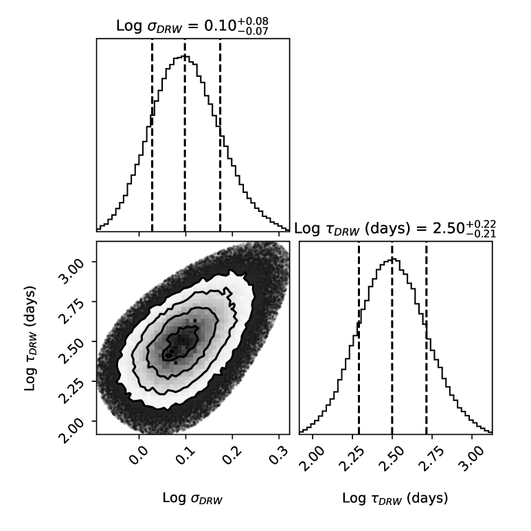
Figure 8: The posterior probability distributions of the DRW model parameters obtained from the modeling of $\gamma$-ray light curve of S5 1803+784 are shown here.

The findings of the modeling of the $\gamma$-ray light curve with DRW model are tabulated in Table 2 and shown in Figures 7, 8. The fit quality is evaluated through the autocorrelation functions of standardized residuals and the square of standardized residuals, Figure 7.

The results from all three approaches are consistent with each other, considering their uncertainties, summarized in Table 3.

Table 2: The observed DRW model parameters from the modeling of $\gamma$-ray light curve of blazar S5 1803+784 are tabulated here.

Source	$\rm{Log}\ \sigma_{DRW}$	$\rm{Log}\ \tau_{DRW}\ (\rm{days})$
(1)	(2)	(3)
S5 1803+784	0.10${}_{-0.07}^{+0.08}$	2.50${}_{-0.21}^{+0.22}$

3.3 Significance estimation

As we discussed, the red noise characteristic of AGN or Blazar’s emissions is believed to originate from stochastic processes and is well represented by a power-law form defined as $P(\nu)\sim A\nu^{-\beta}$, where $\nu$ represents the temporal frequency and $\beta>0$ represents the spectral slope. The best-fitting power-law model slope is $1.03\pm 0.3$. It is crucial to estimate the significance of the dominant peaks obtained from the adopted techniques. In REDFIT analysis Schulz and Mudelsee (2002), the significance was estimated from the $\chi^{2}$ distribution of the periodogram using the equation (8).

Besides the above approach, we used a Monte Carlo simulation approach to estimate the significance of the LSP and WWZ dominant peaks. In this, we simulated the $1\times 10^{5}$ synthetic light curves, having the same PSD and PDF profiles as the original light curve, using the approach of Emmanoulopoulos et al. (2013). We estimated the local significance of observed peaks from the power spectrum distribution at each candidate frequency. In the LSP analysis, the observed peak at $\sim$0.00243 $day^{-1}$ (411 days) has a significance level of 99.7$\%$, while peak at $\sim$0.00251 $day^{-1}$ (399 days) exceeding 99.5$\%$ in WWZ analysis. These findings are consistent with REDFIT analysis and the observed dominant peak frequency is $\sim$0.00237 $day^{-1}$ (421 days with a significance level surpassing 99$\%$. The observed findings confirm the detection of a possible transient quasi-periodic signal in the $\gamma$-ray light curve (MJD 58900 – 60350) with three complete cycles, see the top left panel of Figure 3.

In addition to the previously discussed methodologies for estimating the significance of the observed QPO signal in $\gamma$-ray emissions, we analyzed the $\gamma$-ray light curve using the DRW model. As mentioned earlier, the DRW model is a widely used red noise model capable of characterizing the variability in AGN emissions. Using the EzTao package, we simulated 15,000 mock light curves using the optimal amplitude and damping timescale values with a sampling rate consistent with the real observations. By utilizing the all mock light curves, we computed Lomb-Scargle periodograms for each. To estimate the significance level of the dominant peak in original $\gamma$-ray LSP, we calculated the 84th, 97.5th, 99.85th, and 99.995th percentiles of the 15000 mock LSPs for each candidate frequency value, which correspond to the 1$\sigma$, 2$\sigma$, 3$\sigma$, and 4$\sigma$ significance level. This analysis reveals that the peak at 0.00243 $day^{-1}$ exceeds the 3$\sigma$ significance level. This finding is consistent with the results from other methodologies. We also calculated the spectral window periodogram by constructing a light curve with a total number of time stamps ten times larger than the original one within the observed temporal frame. In this spectral window light curve, the time stamps matching the original observations are assigned a value of one, while all others are set to zero. Further, we applied the LSP method to generate the periodogram, as shown in pink in Figure 9. This analysis highlights that for unevenly sampled time series, the spectral window periodogram can exhibit spurious peaks that arise due to non-uniform sampling in the light curve, have power comparable to the original signal, aiding in the identification of false detections. In our case, the $\gamma$-ray light curve in the given time frame is well sampled and spectral window periodogram did not exhibit any false signals. However, in such studies the results can be influenced by the uneven sampling and finite length of the light curve. Previous studies (Kozłowski, 2017; Suberlak et al., 2021) have demonstrated potential biases in variability measurements due to these limitations. (Burke et al., 2021) found that a valid variability timescale in the light curve should be larger than the mean cadence of the light curve and less than ten percent of the baseline. We adopted this criterion to find out the unreliable regions in the LSP and shaded areas (grey) in Figure 9 represent the invalid regions in the LSP.

In this work, we report a potential transient quasi-periodic oscillation with a period of approximately 411 days, detected in the $\gamma$-ray emission from the blazar S5 1803+784. The signal exceeds a 3$\sigma$ significance level across multiple analysis methods, supporting its authenticity.

Further confirmation of the observed periodic signal, we constructed a phase-folded $\gamma$-ray light curve with a period of $\sim$411 days and fitted it with a sine function, see Figure 5. It further confirms a transient periodic signal in the light curve of blazar S5 1803+784. To enhance the visual clarity, we present two complete periodic cycles within the phase-resolved $\gamma$-ray light curve.

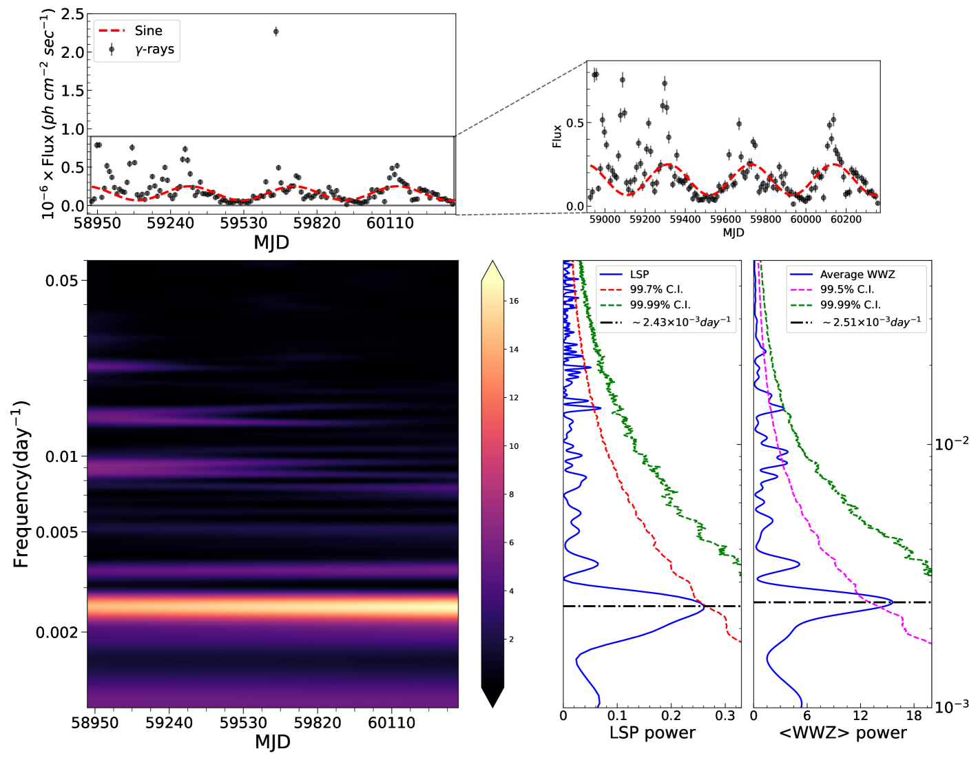
Figure 3: The $\gamma$-ray light curve is analyzed using the Lomb-Scargle Periodogram (LSP) and Weighted Wavelet Z-transform (WWZ) methods. The top-left panel displays the $\gamma$-ray light curve overlaid with a sinusoidal fit. A zoomed-in view of the light curve, excluding the highest flare at around $\sim$59675 MJD (only for clear visibility of the periodic signal), is shown in the top-right panel. The bottom panels present the WWZ map (left), LSP (middle), and average WWZ (right), respectively. The observed local significance of the peak of the timescale of $\sim$411 days from the LSP analysis is $99.7\%$ (red curve) and with a timescale of $\sim$399 days from WWZ analysis is exceeding $99.5\%$.

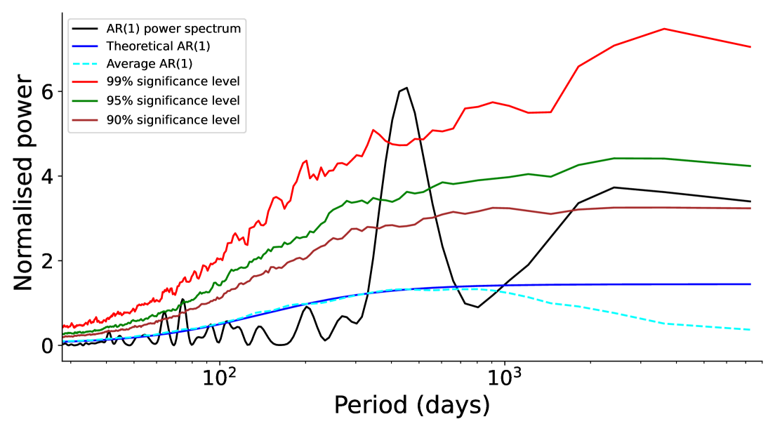
Figure 4: Analysis of the light curve using the AR(1) process with the REDFIT tool. The red noise-corrected power spectrum (black) is presented, alongside theoretical and average AR(1) spectra. The significance levels of 99$\%$, 95$\%$, and 90$\%$ are indicated in red, green, and brown, respectively. A clear transient QPO signature with period of $\sim$421 days is present in the $\gamma$-ray light curve of blazar S5 1803+784.

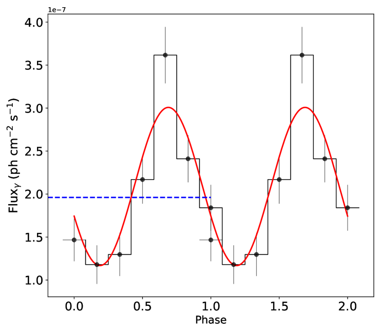
Figure 5: The folded Fermi-LAT light curve (black) of blazar S5 1803+784 in the time domain from MJD 54683 – 60187 above 100 MeV with a period of $\sim$411 days. The dashed blue line represents the mean value and best-fitted sine function to data in red. We present two-period cycles here for better clarity.

Figure 7: The DRW modeling of a 10-day binned $\gamma$-ray light curve of blazar S5 1803+784 over 1400 days from the time stamp MJD 58927. This figure shows the output of modeling, the top panel represents the $\gamma$-ray flux points with their uncertainties, with the best-fit DRW model profile in blue, along with the 1$\sigma$ confidence interval. The bottom panels represent the autocorrelation functions (ACFs) of the standardized residuals (bottom left) and the squared of standardized residuals (bottom right), respectively, along with 95$\%$ confidence intervals of the white noise.

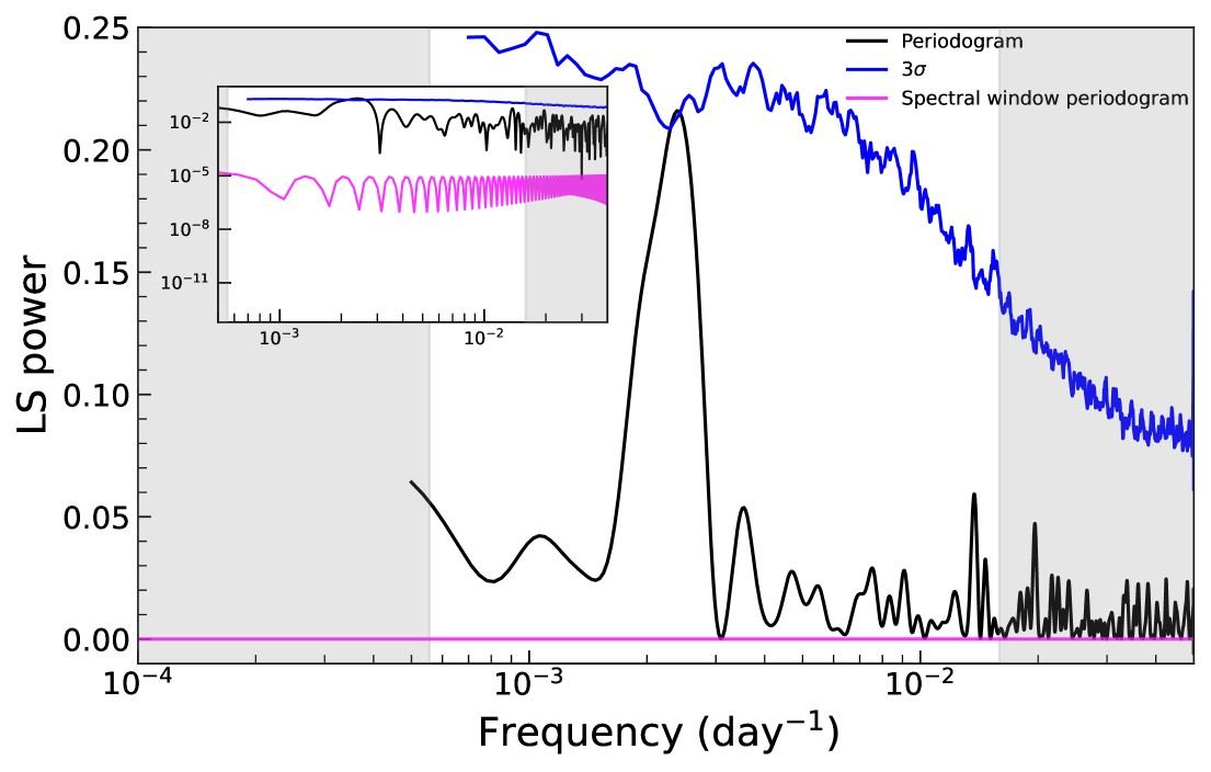
Figure 9: The LSP of the $\gamma$-ray light curve of the blazar S5 1803+784 is shown here. The figure includes the LS periodogram of the original light curves (black) and spectral window (pink). The significance level (blue) of the dominant observed peak in LSP is estimated using DRW mock light curves. The observed peak at 0.00243 $day^{-1}$ exceeds 3$\sigma$ significance level. A logarithmic version of the periodograms is provided in the sub-figure.

Table 3: The transient QPO results obtained using four different approaches are summarized here. Column (1) represents the 4FGL name of the blazar S5 1803+784. Columns (2)–(5) present the transient QPO frequencies derived from the LSP, WWZ, REDFIT, and DCDFT methods, with their uncertainties. The local significance of each QPO is indicated in parentheses next to the corresponding frequency value.

4FGL Name	$10^{-3}\times$  LSP $\left(day^{-1}\right)$	$10^{-3}\times$  WWZ $\left(day^{-1}\right)$	$10^{-3}\times$  REDFIT $\left(day^{-1}\right)$	$10^{-3}\times$  DCDFT $\left(day^{-1}\right)$
(1)	(2)	(3)	(4)	(5)
4FGL J1800.6+7828	2.43$\pm$0.45 ($>99.7\%$)	2.51$\pm$0.2 ($>99.5\%$)	2.37$\pm$0.49 ($>99\%$)	2.51$\pm$0.268

3.4 $\gamma$-ray spectral analysis

We performed $\gamma$-ray spectral analysis using Fermipy’s standard procedure. The log-parabola spectral model was applied to our source of interest, as described by

$$n(E)=K(E/E_{pivot})^{-(\alpha+\beta\log(E/E_{pivot}))}$$ (20)

where $\alpha$ is the photon-index at pivot energy $E_{pivot}=1$ GeV, $\beta$ is the curvature parameter, and K is the normalization. The $\gamma$-ray spectra of the source were fitted using a log-parabola distribution model. The derived parameters are summarized in Table LABEL:table:gamma, while the corresponding spectral shapes for four distinct epochs are illustrated in Figure 10. The reported spectral form of this particular source is also log parabola in the 4FGL Catalog . Although previous studies by Priya et al. (2022) have also shown, that broken power law, and log parabola (LP) are better models to explain $\gamma$-ray SED. Interestingly, we found that states S1 and S2 have large curvature characteristics. Additionally, when the source changed from low to high flux levels, we saw notable shifts in the curvature parameter ($\beta$) and $\alpha_{\gamma}$ . An important feature of our results is the exceptionally steep $\alpha_{\gamma}$ of 2.48 reported between MJD 60125 – 60150. This value surpasses the previous values of 2.27 and 2.29 reported by Omojola and Chen (2021); Priya et al. (2022) respectively. From the four epochs, the photon spectral index values are $\alpha_{\gamma}=1.65$ (S1), $2.10$ (S2), $2.18$ (S3), and $2.48$ (S4). These values are consistent with the earlier findings like classification of Changing-Look Blazars (CLBs) into three states: FSRQ ($\alpha_{\gamma}\gtrsim 2.2$), Transition ($2.0<\alpha_{\gamma}<2.2$), and BL Lac ($\alpha_{\gamma}\lesssim 2.0$) (Ren et al., 2024). Specifically: S1 ($\alpha_{\gamma}=1.65$) falls within the BL Lac state, S2 ($\alpha_{\gamma}=2.10$) and S3 ($\alpha_{\gamma}=2.18$) lie in the Transition state, S4 ($\alpha_{\gamma}=2.48$) corresponds to the FSRQ state. This progression is consistent with Support Vector Machine (SVM) classification, which distinguishes BL Lacs ($\alpha_{\gamma}=2.032\pm 0.212$) from FSRQs ($\alpha_{\gamma}=2.470\pm 0.20$) based on photon spectral index (Fan et al., 2022). Additionally, the density distributions of $\alpha_{\gamma}$ for CLBs (2.0–2.5) lie between BL Lacs and FSRQs, supporting their classification as transitional objects (Kang et al., 2024, 2025).

Table 4: Details of the best fit parameters obtained by $\gamma$-ray spectrum analysis of S5 1803+784 using Fermipy tool. In the table, Columns 1: Observations, 2: Particle distribution models, Parameters: 3, 4, 5, 6, 7, 8: represent the physical parameters corresponding to chosen particle distribution.

Observation	Model	$\alpha$	$\beta$	Norm	$E_{b}$	TS	loglike
(1)	(2)	(3)	(4)	(5)	(6)	(7)	(8)
S1	LP	1.65$\pm$0.41	0.48$\pm$0.33	2.05$\pm$0.52	645.15	69.86	-5774.4496
S2	LP	2.10$\pm$0.08	0.10$\pm$0.05	6.13$\pm$0.55	645.15	112.13	-7937.145
S3	LP	2.18$\pm$0.06	0.02$\pm$0.04	10.81$\pm$0.90	645.15	885.722	-5509.414
S4	LP	2.48$\pm$0.09	0.05$\pm$0.02	6.55$\pm$0.80	645.15	418.494	-5192.92

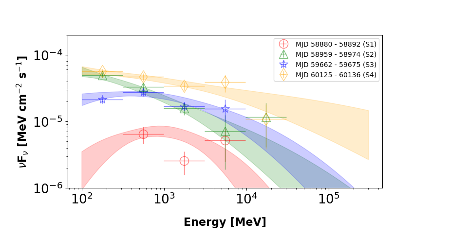
Figure 10: $\gamma$-ray spectral plot using log parabola model

3.5 Broadband spectral analysis

We investigated the broadband spectral features of S5 1803+784, combining Swift-UVOT/XRT and Fermi data. A one-zone leptonic model, incorporating synchrotron and SSC mechanisms, was used to model the spectral energy distribution and constrain its particle energy distribution. So, we assume emission originates from a spherical region of radius R, with the relativistic jet alignment producing Doppler-boosted emission, accounted for by the Doppler factor, $\delta=\frac{1}{\Gamma(1-\beta\,cos\theta)}$. Relativistic particles within the jet lose energy through synchrotron and IC interactions with magnetic fields and photons. For this, we applied the SSC process, utilizing the jet’s own synchrotron photons as seed photons for IC scattering. The electron Lorentz factor, $\gamma$ is expressed in terms of new variable $\xi$, such that $\xi=\gamma\sqrt{\mathbb{C}}$, where $\mathbb{C}=1.36\times 10^{-11}\frac{\delta B}{1+z}$ with z being the redshift of source. The synchrotron flux recieved by the observer with $\xi$ as parameter can be written as (Shah, 2023)

$$F_{syn}(\epsilon)=\frac{\delta^{3}(1+z)}{d_{L}^{2}}V\mathbb{A}\int_{\xi_{min}}^{\xi_{max}}f(\epsilon/\xi^{2})n(\xi)d\xi,$$ (21)

where $\rm d_{L}$ is luminosity distance, V is the volume of emission region, $\rm\mathbb{A}=\frac{\sqrt{3}\pi e^{3}B}{16m_{e}c^{2}\sqrt{\mathbb{C}}}$, $\xi_{min}$ and $\xi_{max}$ correspond to the minimum and maximum energy of electron, and f(x) is the synchrotron emmisivity function (Rybicki and Lightman, 1986). The SSC flux received by the observer at energy $\epsilon$ can be obtained using the equation

$$\begin{split}F_{ssc}(\epsilon)=\frac{\delta^{3}(1+z)}{d_{L}^{2}}V\mathbb{B}\epsilon&\int_{\xi_{min}}^{\xi_{max}}\frac{1}{\xi^{2}}\int_{x_{1}}^{x_{2}}\frac{I_{syn}(\epsilon_{i})}{\epsilon_{i}^{2}}\\ &f(\epsilon_{i},\epsilon,\xi/\sqrt{\mathbb{C}})d\epsilon_{i}n(\xi)d\xi\end{split}$$ (22)

where, $\rm\epsilon_{i}$ is incident photon energy, $\rm\mathbb{B}=\frac{3}{4}\sigma_{T}\sqrt{\mathbb{C}}$, $\rm I_{syn}(\epsilon_{i})$ is the synchrotron intensity, $\rm x_{1}=\frac{\mathbb{C}\,\epsilon}{4\xi^{2}(1-\sqrt{\mathbb{C}}\,\epsilon/\xi m_{e}c^{2})}$, $\rm x_{2}=\frac{\epsilon}{(1-\sqrt{\mathbb{C}}\,\epsilon/\xi m_{e}c^{2})}$ and

$$f(\epsilon_{i},\epsilon,\xi)=2q\log q+(1+2q)(1-q)+\frac{\kappa^{2}q^{2}(1-q)}{2(1+\kappa q)}$$

here $\rm q=\frac{\mathbb{C}\epsilon}{4\xi^{2}\epsilon_{i}(1-\sqrt{\mathbb{C}}\epsilon/\xi m_{e}c^{2})}$ and $\rm\kappa=\frac{4\xi\epsilon_{i}}{\sqrt{\mathbb{C}}m_{e}c^{2}}$.

We numerically solve Equations 21 and 22, and integrate the resulting code as a local convolution model in XSPEC. In the convolved XSPEC model ‘energy’ variable is interpreted as $\xi=\gamma\sqrt{\mathbb{C}}$. This convolution model allows for statistical fitting of broadband SEDs, making it possible to model broadband spectra for any given particle energy distribution $n(\xi)$. Within this region, we consider a relativistic particle distribution denoted as n(E). However, Broken power law (BPL) distribution provides reasonable parameters for the broadband SED modeling. The BPL distribution is given by

$$n(E)=\begin{cases}KE^{-p_{1}}&\text{for }E<E_{b}\\ KE_{b}^{p_{2}-p_{1}}E^{-p_{2}}&\text{for }E\geq E_{b}\end{cases}$$ (23)

where $K$ is normalization, $E_{\rm b}$ is break energy, $p_{1}$ and $p_{2}$ indicate the particle indices before and after break energy $E_{\mathrm{b}}$.

In the broadband spectral energy distribution (SED) modeling, key parameters such as the bulk Lorentz factor ($\Gamma$), magnetic field strength (B), size of the emission region (R), and jet opening angle ($\theta$) play a crucial role. In the context of BPL model, which is characterized by four parameters like spectral indices before and after the break ($p_{1}$ and $p_{2}$), the break energy $E_{\mathrm{b}}$, and the normalization factor (Norm), the normalization factor is typically treated as a free parameter during the fitting process. Initial values for these parameters are chosen based on the observed spectral shapes and flux levels of the synchrotron and SSC components. These parameters are then iteratively varied to converge on their optimal values, ensuring a good fit to the data. The broadband SED fitting code also allows for the inclusion of the jet power ($P_{jet}$) as one of the parameters. Adopting the standard approach, where cold protons and non-thermal electrons equally contribute to jet inertia, we derived an estimate of the total jet power formula by Ghisellini et al. (2014)

$$P_{\text{jet}}=\pi R^{2}\Gamma^{2}\beta cU_{e}$$ (24)

where We denote $\Gamma$ as the bulk Lorentz factor, $\beta=\frac{v}{c}$ as the jet velocity (v/c), R as the jet radius, and $U_{e}$ as the energy densities of electrons respectively.

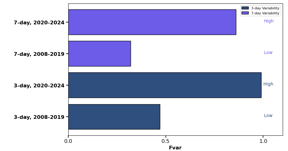
Figure 11: Fractional variability $(F_{var})$ in different flux states and time bins for $\gamma$-ray data. The $F_{var}$ values are calculated for various flux states, including the low-flux (LFS) and high-flux (HFS). The time bins considered are 3-day and 7-day bins.

Table 5: The table presents the optimal parameters obtained by fitting the broadband spectrum of S5 1803+784 using a one-zone SED model in XSPEC. The columns represent: (1) Observation details, (2) Particle distribution models used, (3) Bulk Lorentz factor, (4-6) Parameters corresponding to the chosen particle distribution, (7) Magnetic field strength (in Gauss), (8) Logarithmic jet power (in erg $sec^{-1}$), and (9) Reduced-$\chi^{2}$. Subscript and superscript values indicate lower and upper bound errors, respectively. A dash (–) indicates that the lower or upper bound error is unconstrained.

Observation	Model	$\Gamma$	$p_{1}$	$p_{2}$	log R(cm)	B(G)	$P_{jet}$	$\chi^{2}_{red}$
(1)	(2)	(3)	(4)	(5)	(6)	(7)	(8)	(9)
S1	BPL	$14.90^{+0.48}_{-0.37}$	$1.24^{+0.12}_{-0.20}$	$4.34^{+0.34}_{-0.22}$	16.0	$0.26^{+0.03}_{-0.02}$	$43.40^{+0.20}_{-0.17}$	0.82
S2	BPL	$30.36^{-}_{-0.60}$	$2.18^{+0.06}_{-0.06}$	$5.27^{+0.85}_{-0.21}$	16.0	$0.26^{+0.04}_{-0.03}$	$46.03^{-}_{-0.80}$	1.16
S3	BPL	$22.56^{+0.52}_{-0.43}$	$1.97^{+0.02}_{-0.03}$	$4.99^{+0.37}_{-0.29}$	16.0	$0.05^{+0.003}_{-0.002}$	$45.85^{+0.25}_{-0.29}$	1.09
S4	BPL	$21.52^{+0.22}_{-0.17}$	$1.10^{+0.05}_{-0.05}$	$4.85^{+0.15}_{-0.12}$	16.0	$0.19^{+0.02}_{-0.01}$	$45.36^{+0.16}_{-0.13}$	0.56

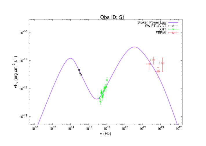
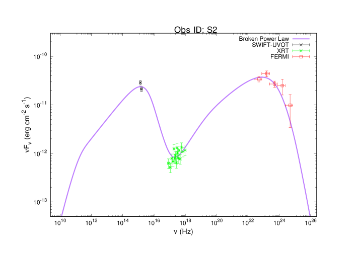
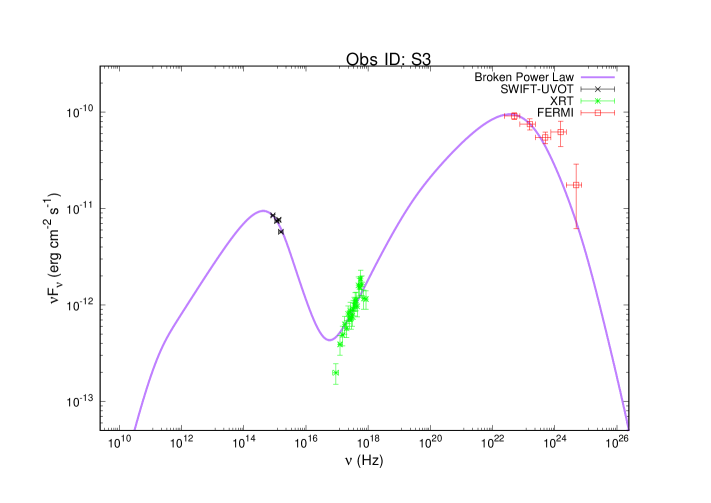
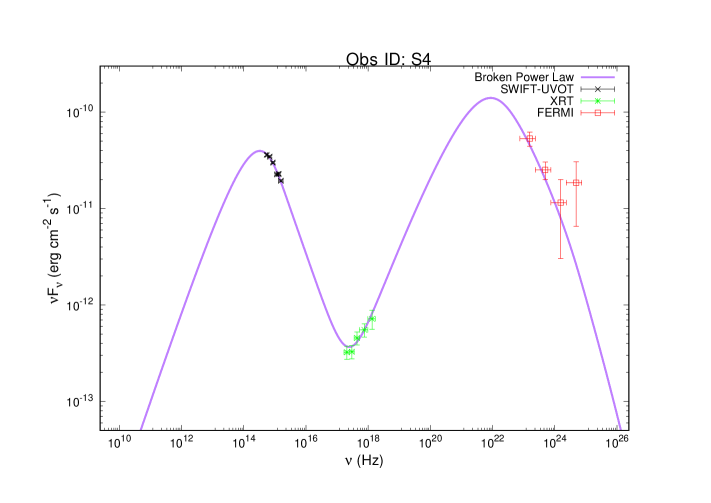
Figure 12: The following plots show the broadband spectral energy distributions (SEDs) for four distinct epochs (S1-S4) using the Broken Power Law (BPL) particle distribution model

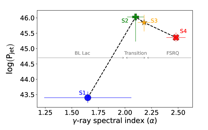
Figure 13: Jet power ($\log P_{\rm jet}$) as a function of $\gamma$-ray spectral index ($\alpha$) across four observational epochs: S1, S2, S3, and S4. The photon spectral index starts at 1.65 in S1 and progressively increases through subsequent epochs: 2.10 in S2, 2.18 in S3, and 2.48 in S4. This trend suggests that the blazar S5 1803+784 may be undergoing a transition from a BL Lac to FSRQ.

4 Summary and Discussion

The transition blazar S5 1803+784 offers a unique opportunity to explore blazar physics due to its remarkable ability to shift between various activity phases. This characteristic has made it a continuous subject of study, with several multi-wavelength investigations conducted during periods of flaring activity. However, simultaneous X-ray/UV/Optical data have been limited Priya et al. (2022); Omojola and Chen (2021), highlighting the need for further analysis. This study offers a detailed temporal and spectral analysis of S5 1803+784, exploring both its quiet and flaring states, and uncovering its underlying properties. Notably, we observed the highest $\gamma$-ray flux of ($\mathrm{2.26\pm 0.062)\times 10^{-6}~phcm^{-2}s^{-1}}$ MJD 59667.29 – 59676.03. Temporal analysis of $\gamma$-ray data revealed striking correlations between activity levels and flux fluctuations. Variability is crucial in understanding blazar structure, as it can arise from intrinsic factors. Intrinsic mechanisms involve fluctuations in particle injection or acceleration within specific jet regions, such as the base or shock front. These fluctuations are amplified by shock interactions and magnetic field changes, leading to pronounced observed flux variations due to Doppler boosting. Our analysis revealed significant variability factors in both 3-day and 7-day binned light curves. Specifically, the three-day binned light curve displayed a variability factor of 0.47 ± 0.03 between 2008-2019, increasing to 0.99 ± 0.03 during 2020-2024. Similarly, the seven-day binned light curve showed variability factors of 0.32 ± 0.06 and 0.86 ± 0.05 for the same periods as shown in Figure 11. Surprisingly, X-ray emissions during the period (2020-2023) were lower than UV/optical and $\gamma$-ray wavelengths, diverging from BL Lac behavior. As high-energy electrons characterized by rapid cooling, generate substantial variability in the Optical/UV and $\gamma$-ray domains. In contrast, the more gradual cooling of lower-energy electrons leads to reduced variability in the X-ray domain. But in the case of BL Lacs, X-ray fluctuations show greater amplitude than those in $\gamma$-ray and optical regimes, even when the source is in a low-flux state Kapanadze et al. (2023); Abe et al. (2023, 2024). The unusual behavior hints at Low-energy-peaked BL Lac (LSP) characteristics, resembling Flat Spectrum Radio Quasar (FSRQ) properties. The lower variability observed in the X-ray band compared to the optical and gamma-ray bands suggests characteristics of a Low-energy-peaked BL Lac (LSP). This behavior can be explained by the shape of the SED in LBLs, where the X-ray emission lies near the lower energy tail of the synchrotron self-Compton (SSC) component. In LBLs, the X-ray emission is primarily produced by lower energy electrons in the jet. These electrons have longer cooling timescales compared to higher energy electrons, as cooling time is directly proportional to electron energy. Higher energy electrons, responsible for optical and gamma-ray emission, lose energy more rapidly through synchrotron and inverse Compton processes, leading to faster variability in these bands. In contrast, the slower cooling of lower energy electrons results in more stable and less variable X-ray emission. Recent studies on the transition blazar B2 1308+326 by Pandey et al. (2024) reveal lower X-ray emission compared to optical and $\gamma$-ray bands, aligning with our findings and demonstrating a similar trend in X-ray emission behavior. Examining the structure of fractional variability across different energy levels can provide significant insights into the particle population or processes generating broadband emissions. This study highlights the importance of continued multi-wavelength monitoring of S5 1803+784 to understand its unique characteristics further to understand the underlying physics of transition blazars.

In addition, A transient quasi-periodic oscillation with a period of $\sim$411 days was identified using multiple methods, including the Lomb-Scargle Periodogram, Weighted Wavelet Z-Transform, and REDFIT analysis. The results from all approaches are consistent and mutually supportive within their error bars. The detection significance of the periodic signals exceeded 99$\%$ across all methods, affirming the authenticity of the signal.

The production mechanism of quasi-periodic oscillations in AGN remains a subject of debate. However, several intriguing physical models have been proposed to explain the observed phenomena. Among these, the supermassive binary black hole (SMBBH) system has been notably successful in accounting for the $\sim$12 yr QPO observed in OJ 287. This model has since been widely adopted to explain other stable, long-term QPOs Valtonen et al. (2008); Villforth et al. (2010). In addition to the SMBBH model, other models such as continuous jet precession and Lense-Thirring precession of the accretion disk have been proposed to explain long-duration QPOs Romero et al. (2000); Rieger (2004); Stella and Vietri (1997); Liska et al. (2018); You et al. (2018). But for transient QPOs, which persist for a few cycles, alternative physical models need to be considered. One possibility involves hotspots orbiting within the innermost stable circular orbit (ISCO) of an SMBH. The motion of the hotspots can modulate the seed photon field for the external inverse Compton scattering (EC) within the jet, resulting in periodic gamma-ray emission Zhang and Bao (1990); Gupta et al. (2008). Another potential mechanism involves magnetic reconnection events, where periodically spaced magnetic islands within the jet drive the QPOs of the BH systems at various scales Huang et al. (2013). It is necessary to explore other mechanisms that might be more favorable for such observed transient quasi-periodic signatures.

The helical motion of an enhanced emission region (or blob) within the jet has been extensively studied in the context of transient QPOs during flares, e.g. Mohan and Mangalam (2015); Sobacchi et al. (2016); Zhou et al. (2018) In the one-zone leptonic model, blazar emission primarily originates from this emission region (or blob) in the jet. High-energy gamma-ray emission is produced via the synchrotron self-Compton (SSC) process. A helical jet structure can arise due to large-scale magnetic fields or hydrodynamic effects that induce helical motion in the jet or its emission region (or blob) Mohan and Mangalam (2015); Sobacchi et al. (2016); Sarkar et al. (2021). Periodic fluctuations in the observed emission are attributed to variations in the Doppler boosting factor as the viewing angle of the moving plasma blob changes. The variability timescale, influenced by factors such as the Doppler boosting factor, pitch angle, and viewing angle, can span from a few days to several months.

In this model, the periodic changes in the viewing angle ($\theta$) are driven by the helical motion of the emission region, defined as

$$\rm{cos}\ \theta_{obs}(t)=\rm{sin\phi}\ \rm{sin\psi}\ \rm{cos(2\pi t/P_{obs})}+\rm{cos\phi}\ \rm{cos\psi}$$ (25)

where P_obs is the observed periodicity, $\phi$ is the pitch angle of the blob, and $\psi$ is the viewing angle or inclination angle measured between the line of sight of the observer and the jet axis. The varying Doppler factor is defined as $\delta=\frac{1}{\Gamma\left[1-\beta\rm{cos\theta_{obs}(t)}\right]}$, where $\Gamma=1/\sqrt{1-\beta^{2}}$ represents the bulk Lorentz factor associated with the motion of blob, and $\beta=\it{v_{jet}}/c$. In the case BL Lac, considered values of $\phi=2^{\circ}$, $\psi=5^{\circ}$, and $\Gamma=8.5$, Abdo et al. (2010a); Sobacchi et al. (2016); Zhou et al. (2018); Sarkar et al. (2021); Sharma et al. (2024a); Chen et al. (2024). The relation between the observed and rest-frame periods is defined as

$$P_{rest}=\frac{P_{obs}}{1-\beta\ \rm{cos\phi}\ \rm{cos\psi}}$$ (26)

The estimated $\beta$ value using the expression of $\Gamma$ is 0.99305. The translated period value in the rest frame of the blob is $P_{rest}\sim$ 99.3 yr for the $P_{obs}$=411 days and the distance traveled by the blob in one cycle is $D_{1P}=c\ \beta\ P_{rest}\ cos\phi\approx 30.18pc$ and the projected distance for entire transient phase is $D_{projected}=N\ D_{1P}\ sin\psi\approx 7.87pc$. The extended jets with parsec-scales have been identified in numerous blazars Bahcall et al. (1995); Vicente et al. (1996); Tateyama et al. (1998), and the study is supported by the optical polarization observations highlighting the evidence of the presence of helical structures Marscher et al. (2008). However, the exact origin of their helical structure remains unclear. Further, a modified helical jet model might be a more robust mechanism to explain such features, in which a blob moves helically inside a time-varying jet. In this model, the inclination angle between the jet axis and the line of sight could be time dependent, $\psi\equiv\psi(t)$ Sarkar et al. (2021); Prince et al. (2023). The variation in the angle could be attributed to the periodic modulations in observed emissions and outliers (high flux points) within the light curve could be associated with some stochasticity present in the jets. In this investigation, the conclusion is that the helical magnetic field could play a key role in shaping these jet structures. Chen et al. (2024) noticed that the transient QPOs are more commonly observed in FSRQ than BL Lac. A distribution of sources belonging to different blazar classes reported as a transient QPO source is given in Figure 14 and detailed in Table 7, 8.

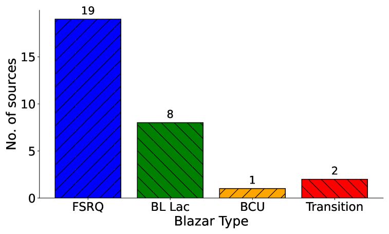
Figure 14: Distribution of reported transient quasi-periodic oscillations (QPOs) observed in different classes of blazar in the literature Table 8, with timescales ranging from days to years. The figure categorizes sources based on their type, including Flat Spectrum Radio Quasars (FSRQs), BL Lacs, Blazar Candidates of Uncertain Type (BCUs), and transition blazar from BL Lac to FSRQ.

The Fermi-LAT detection of various blazar types, including Low-Synchrotron-Peaked (LSP), Intermediate-Synchrotron-Peaked (ISP), and High-Synchrotron-Peaked (HSP) blazars, has significantly advanced our understanding of these enigmatic objects Ackermann et al. (2015b). However, a substantial fraction of LSP blazars remain undetected, suggesting that they may possess distinct properties that hinder their detection. In fact, research suggests that these undetected LSP blazars may constitute a distinct class of “$\gamma$-ray quiet blazars” characterized by lower polarization and notable radio brightness, as evidenced by optical polarization properties and radio emission Angelakis et al. (2016). This phenomenon is attributed to the steep $\gamma$-ray photon spectral index of LSP blazars, which poses a significant detection challenge Ackermann et al. (2015b); Paliya et al. (2020). Furthermore, this effect is exacerbated for high-redshift sources, where the $\gamma$-ray spectral energy distribution (SED) is shifted to lower frequencies in the observer’s rest frame. In addition, the study suggests that the lower synchrotron peak blazars (LSPs) could be the source of changing-look blazars (CLB)(BL Lac to FSRQ) because 90.7 percent of the CLB are found to be LSP Xiao et al. (2022); Kang et al. (2023). Recently, a study by Ren et al. (2024), investigated the evolution of Changing-Look Blazars (CLBs) on long timescales, classifying them into three morphological types: FSRQ, Transition, and BL Lac states, based on the relationship between emission line equivalent width and $\alpha_{\gamma}$ photon spectral index, revealing distinct $\alpha_{\gamma}$ ranges for each state found that $\alpha_{\gamma}$ satisfy the relationships with $\alpha_{\gamma}$ $\gtrsim$ 2.2 for the FSRQ state, $2.0<\alpha_{\gamma}<2.2$ for the transition state, and $\alpha_{\gamma}$ $\lesssim$ 2.0 for the BL Lac state. Alternatively, the $\gamma$-ray spectrum of the source follows a power-law distribution: $N_{\nu}=A\nu^{-a}$ with $\alpha_{\gamma}$ = 2.26 ± 0.02, indicating a transitional state between FSRQs and LSP (BL Lacs), detected with Fermi-LAT observations Ajello et al. (2020); Nesci et al. (2021). Earlier, a study has found that $\gamma$-ray sources detected by Fermi-LAT tend to have exceptionally high jet speeds, corresponding to large bulk Lorentz factors Lister et al. (2009, 2015). It also suggested that LSP blazars with low Lorentz factors and synchrotron peaks below $10^{13.4}$ Hz are less likely to be $\gamma$-ray detectable. Furthermore, a comprehensive analysis of LSP blazars was performed to determine key characteristics, including Compton dominance, peak powers of synchrotron and inverse Compton radiation, and frequency distributionsArsioli and Polenta (2018). In our work, the $\gamma$-ray spectral analysis of S5 1803+784 shows $\alpha_{\gamma}$ = 2.48 and Compton dominance (CD), indicating a characteristic property of FSRQ sources. Alternatively, a steep $\gamma$-ray slope indicates that the decrease in radiative cooling allowed relativistic particles to accelerate to higher energies, resulting in a corresponding shift in the peaks of the synchrotron and IC components. Also, the $\gamma$-ray spectra of FSRQs are generally softer, and their variability is stronger than those of BL Lacs, confirming earlier studies by Ajello et al. (2020). The jet power against the $\alpha_{\gamma}$ is given in Figure 13, a remarkable evolutionary trend is uncovered in the blazar S5 1803+784, as its jet power correlates with a steady increase in $\alpha_{\gamma}$ across four observational epochs (S1-S4). From an initial index of 1.65 in S1, the photon spectral index rises progressively to 2.10, 2.18, and ultimately 2.48 in S4. This sustained shift implies a profound change in the blazar properties, possibly indicating a transition from a BL Lac object to an FSRQ. The jet power values and $\alpha_{\gamma}$ are given in Table LABEL:table:gamma,5. Recent work employed Support Vector Machine (SVM) classification to distinguish between BL Lac objects and Flat Spectrum Radio Quasars (FSRQs) based on photon spectral index and photon flux (Fan et al., 2022). The average $\alpha_{\gamma}$ = 2.470 ± 0.201 for 795 FSRQs and $\alpha_{\gamma}$ = 2.032 ± 0.212 for 1432 BL Lacs. Contemporary, Kang et al. (2024, 2025), the density distributions of the $\alpha_{\gamma}$ were analyzed for a sample of 2250 blazars, including 1397 BL Lacs, 105 CLBs (classified as intermediate blazars), and 748 FSRQs using the Gaussian mixture modeling clustering algorithm. The results revealed that the density distributions of CLBs in terms of $\alpha_{\gamma}$ are distinctly positioned between those of BL Lacs and FSRQs. Specifically, the values of $\alpha_{\gamma}$ for CLBs were found to lie predominantly in the range of 2.0 to 2.5, indicating an intermediate spectral behavior between the harder spectra of BL Lacs and the softer spectra of FSRQs. This finding supports the classification of CLBs as transitional objects bridging the gap between BL Lacs and FSRQs in terms of their spectral properties.These results collectively emphasize the importance of considering the photon spectral index and other properties to understand blazar diversity.

We applied a leptonic one-zone model to the broadband spectral energy distribution (SED) of S5 1803+784, incorporating both synchrotron and Synchrotron Self-Compton (SSC) effects. Notably, our broadband SED modeling reveals that the SSC model accurately reproduces the observed flux states within this framework, without requiring external Compton contributions. This approach offers several advantages, including seamless integration with XSPEC, enabling reliable and precise statistical analysis, and tightly constrained model parameters Tantry et al. (2024). Consequently, multiband observations of blazars facilitate a comprehensive understanding of their flux and spectral evolution. These observations provide critical insights into the spatial structure, dynamics, and electron cooling processes within relativistic jets, thereby enabling rigorous testing of theoretical frameworks. Notably, previous broadband SED analyses revealed that S5 1803+784 shifted from a low-synchrotron-peaked (LSP) state to an intermediate-synchrotron-peaked (ISP) state during a flare, suggesting the presence of highly energetic particles or a decrease in Compton dominance (CD) Omojola and Chen (2021). This transition caused X-ray emission to shift from inverse Compton scattering to the high-energy tail of synchrotron emission. Alternatively, for another transition blazar B2 1308+326, the same trend is followed by X-ray emission during the flaring state. But in the case of the quiescent state, the X-ray emission occurs at the low energy tail of the inverse Compton, which indicates CD Ajello et al. (2020). However, detecting LSP and ISP blazars in the hard X-ray band poses challenges due to the presence of a spectral valley between the low- and high-energy humps (Böttcher, 2007). Despite these challenges, our multi-wavelength SED modeling suggests different trends across four epochs, as depicted in Table 5. Our derived bulk Lorentz factor and photon indices generally agree with previous studies using the jet-set model. However, our study indicates X-ray emission falls within the lower energy range of the inverse Compton scattering spectrum in its quiescent state (S1, S3). Alternatively, during the flaring state (S2, S4) X-ray emission shifts from inverse Compton scattering to the high-energy tail of synchrotron emission. A previous study by Priya et al. (2022); Omojola and Chen (2021) did not investigate X-ray emission behavior during quiescent and flaring states. Consistent with Liodakis et al. (2017), our independent SED modeling yields a Doppler factor of 21.5. This finding underscores the importance of understanding the bulk Lorentz factor in interpreting changes in jet power. The emission from blazars during outbursts is primarily attributed to relativistic shocks propagating through the jet. As shocks traverse the relativistic jet plasma, they boost nonthermal emission through Doppler enhancement, consistent with the theoretical framework established by Blandford and Königl (1979). Blazars offer a unique opportunity to study relativistic jets, supermassive black holes (SMBHs), and accretion disks. To study jet power, consideration of the magnetic field, emission region size, and $\gamma_{min}$ is crucial (Tantry et al., 2024). Further observational and theoretical studies are necessary to understand the mechanisms driving these phenomena fully.

5 Acknowledgements

We sincerely thank the anonymous referees for their valuable feedback and suggestions, which have significantly improved the quality of our manuscript.The authors acknowledges the support of Prof. Ranjeev Misra in obtaining the Convolution codes used in this work . J. Tantry, Z. Shah and N. Iqbal are thankful to the Indian Space Research Organisation, Department of Space, Government of India (ISRO-RESPOND, , DS$\_$2B-13013(2)/8/2020-Sec.2) for the financial support. ZS is supported by the Department of Science and Technology, Govt. of India, under the INSPIRE Faculty grant (DST/INSPIRE/04/2020/002319). We express our gratitude to the Inter-University Centre for Astronomy and Astrophysics (IUCAA) in Pune, India, for the support and facilities provided. A. Sharma is grateful to Prof. Sakuntala Chatterjee at S.N. Bose National Centre for Basic Sciences, for providing the necessary support to conduct this research.

Appendix A Supplementary Data

Swift observations.

S. No.	Instrument	Observation ID	Time (MJD)	XRT exposure (ks)	UVOT exposure (ks)
1.	Swift-XRT/UVOT	00095124013	58748.03	1.14	1.14
2.	Swift-XRT/UVOT	00036393021	58957.05	1.87	1.86
3.	Swift-XRT/UVOT	00036393020	58954.01	1.98	1.98
4.	Swift-XRT/UVOT	00095124027	58804.5	1.57	1.57
5.	Swift-XRT/UVOT	00095124025	58797.2	1.50	1.49
6.	Swift-XRT/UVOT	00095124023	58790.07	1.22	1.22
7.	Swift-XRT/UVOT	00095124028	58808.04	0.97	0.96
8.	Swift-XRT/UVOT	00095124033	58829.12	1.46	1.45
9.	Swift-XRT/UVOT	00095124036	58839.66	1.42	1.41
10.	Swift-XRT/UVOT	00095124034	58832.31	1.38	1.38
11.	Swift-XRT/UVOT	00095124038	58846.30	1.29	1.28
12	Swift-XRT/UVOT	00095124040	58853.00	1.15	1.15
13	Swift-XRT/UVOT	00095124041	58857.91	0.92	0.91
14.	Swift-XRT/UVOT	00095124044	58874.74	1.11	1.10
15.	Swift-XRT/UVOT	00095124037	58843.25	1.26	1.25
16.	Swift-XRT/UVOT	00095124030	58818.51	1.26	1.25
17.	Swift-XRT/UVOT	00095124032	58825.08	1.23	1.22
18.	Swift-XRT/UVOT	00095124035	58836.02	1.20	1.19
19.	Swift-XRT/UVOT	00095124031	58822.8	1.19	1.18
20.	Swift-XRT/UVOT	00095124042	58860.03	1.12	1.11
21.	Swift-XRT/UVOT	00095124045	58878.33	1.22	1.23
22.	Swift-XRT/UVOT	00095124047	58885.22	1.10	1.09
23.	Swift-XRT/UVOT	00095124048	58888.00	1.22	1.22
24.	Swift-XRT/UVOT	00095124049	58892.00	1.25	1.25
25.	Swift-XRT/UVOT	00095124050	58895.03	1.23	1.23
26.	Swift-XRT/UVOT	00095124051	58899.61	0.10	0.09
27.	Swift-XRT/UVOT	00095124052	58902.73	1.27	1.26
28.	Swift-XRT/UVOT	00095124053	58906.64	1.18	1.17
29.	Swift-XRT/UVOT	00095124054	58909.10	1.18	1.17
30.	Swift-XRT/UVOT	00095124055	58913.08	1.13	1.12
31.	Swift-XRT/UVOT	00095124056	58920.70	0.94	0.93
32.	Swift-XRT/UVOT	00095124057	58923.49	1.43	1.42
33.	Swift-XRT/UVOT	00095124058	58927.79	1.10	1.09
34.	Swift-XRT/UVOT	00095124059	58930.31	1.37	1.36
35.	Swift-XRT/UVOT	00095124060	58934.03	0.41	0.40
36.	Swift-XRT/UVOT	00095124061	58934.03	1.19	1.18
37.	Swift-XRT/UVOT	00036393022	59667.29	1.19	1.18
38.	Swift-XRT/UVOT	00036393023	59669.15	1.91	1.90
39.	Swift-XRT/UVOT	00036393024	59670.60	1.91	1.90
40.	Swift-XRT/UVOT	00036393025	59676.03	2.11	2.12
41.	Swift-XRT/UVOT	00036393026	60123.87	1.67	1.64
42.	Swift-XRT/UVOT	00036393027	60127.31	0.33	0.33
43.	Swift-XRT/UVOT	00036393028	60131.20	1.24	1.21

Table 6: The list of Swift-XRT/UVOT observations used in this work is shown above. All observations are accessible

Source name	4FGL name	Source class	Light curve binning	QPO period	QPO cycle number	Reference
			(days)	(days)
(1)	(2)	(3)	(4)	(5)	(6)	(7)
B2 1520+31	4FGL J1522.1+3144	FSRQ	7	179$\pm$42	6	a
			7, 3	71$\pm$15	14	a,b
			7	39$\pm$11	17	a
PKS 1510-089	4FGL J1512.8-0906	FSRQ	0.125	3.6$\pm$0.07	5	c
			7	92$\pm$1.2	7	c
3C 454.3	4FGL J2253.9+1609	FSRQ	1	47${}_{-0.51}^{+0.97}$	9	d
3C 279	4FGL J1256.1-0547	FSRQ	7	39$\pm$1	–	e
			7	24$\pm$1	–	e
4C +01.02	4FGL J0108.6+0134	FSRQ	7	122$\pm$26	5	a
			7	268$\pm$54	4	a
PKS 0402-362	4FGL J0403.9-3605	FSRQ	7	122$\pm$42	5	a
			7	221$\pm$60	3	a
4C +21.35	4FGL J1224.9+2122	FSRQ	7	66$\pm$17	6	a
PKS 1424-41	4FGL J1427.9-4206	FSRQ	7	57.1$\pm$4.5	5	g
			7	90$\pm$22	5	a
			10	$\sim$355	–	f
CTA	4FGL J2232.6+1143	FSRQ	7	178$\pm$40	5	a
			7	366$\pm$81	3	a
			0.125	7.6${}_{-0.25}^{+0.36}$	8	h
PKS 0336-01	4FGL J0339.5-0146	FSRQ	7	94.6$\pm$6.8	6	g
PKS 2255-282	4FGL J2258.1-2759	FSRQ	7	93$\pm$2.6	–	i
PKS 0346-27	4FGL J0348.5-2749	FSRQ	1	100	–	j
S5 1044+71	4FGL J1048.4+7143	FSRQ	7	1127$\pm$226	3	a
			7	117$\pm$38 (7d LC)	4	a
4C +28.07	4FGL J0237.8+2848	FSRQ	7	244$\pm$88	3	a
PKS 0454-234	4FGL J0457.0-2324	FSRQ	7	69$\pm$21	4	a
3C 273	4FGL J1229.0+0202	FSRQ	7	177$\pm$38	4	a
			7	97$\pm$25	3	a
PMN J2345-1555	4FGL J2345.2-1555	FSRQ	7	191$\pm$44	4	a
PKS 0244-470	4FGL J0245.9-4650	FSRQ	10	225$\pm$24	8	k
4C +38.41	4FGL J1635.2+3808	FSRQ	10	110$\pm$50	4.2	k
			10	60$\pm$9	5.4	k
			10	19$\pm$2	5.1	k
			10	35$\pm$4	5.3	k
			10	104$\pm$7	6	k
			10	$\sim$227	3.7	k

Table 7: A list of reported transient QPOs in blazars in the literature (Part 1).

Source name	4FGL name	Source class	Light curve binning	QPO period	QPO cycle number	Reference
			(days)	(days)
(1)	(2)	(3)	(4)	(5)	(6)	(7)
PKS 0426-380	4FGL J0428.6-3756	BL Lac	7	85$\pm$26	8	a
PKS 0447-439	4FGL J0449.4-4350	BL Lac	7	111$\pm$42	7	a
S5 0716+714	4FGL J0721.9+7120	BL Lac	7	324$\pm$77	5	a
			5	31.3$\pm$1.8	7	l
1H 1013+498	4FGL J1015.0+4926	BL Lac	7	52$\pm$12	12	a
			7	100$\pm$25	4	a
			7	264$\pm$59	4	a
Mrk 501	4FGL J1653.8+3945	BL Lac	7	326$\pm$76	7	a
PKS 0537-441	4FGL J0538.8-4405	BL Lac	7	55$\pm$3.3	7	g
			7	54.7$\pm$3.3	7	g
PKS 2155-304	4FGL J2158.8-3013	BL Lac	7	341$\pm$106	4	a
Mrk 421	4FGL J1104.4+3812	BL Lac	7	300$\pm$65	3	a
PKS 2247-131	4FGL J2250.0-1250	BCU	5	34.5$\pm$1.5	6	m
			7	214$\pm$43	6	a
S4 0954+658	4FGL J2345.2-1555	Transition blazar	10	66$\pm$4.8	9	n
			10	208$\pm$43	5	n
S5 1803+784	4FGL J1800.6+7828	Transition blazar	3	$411\pm 79$	3	Our study

Table 8: Continued from Table 7. Column (1) is the name of object; Column (2) is the Fermi 4FGL name; Column (3) is the source class type; Column (4) is the transient QPO timescale and associated uncertainty in days; Column (5) is the QPO cycle number; Column (6) is the reference: (a) Ren et al. (2023), (b) Gupta et al. (2019), (c) Roy et al. (2022), (d) Sarkar et al. (2021), (e) Sandrinelli et al. (2016), (f) Yang et al. (2021), (g) Chen et al. (2024), (h) Sarkar et al. (2020), (i) Sharma et al. (2024a), (j) Prince et al. (2023), (k) Das et al. (2023), (l) Chen et al. (2022), (m) Zhou et al. (2018), (n)Gong et al. (2023)

References

- Abdo et al. (2010a) Abdo, A., Ackermann, M., Agudo, I., Ajello, M., Aller, H., Aller, M., Angelakis, E., Arkharov, A., Axelsson, M., Bach, U., et al., 2010a. The spectral energy distribution of fermi bright blazars. The Astrophysical Journal 716, 30.
- Abdo et al. (2010b) Abdo, A., Ackermann, M., Ajello, M., Antolini, E., Baldini, L., Ballet, J., Barbiellini, G., Bastieri, D., Bechtol, K., Bellazzini, R., et al., 2010b. Gamma-ray light curves and variability of bright fermi-detected blazars. The Astrophysical Journal 722, 520.
- Abe et al. (2023) Abe, H., Abe, S., Acciari, V.A., Agudo, I., Aniello, T., Ansoldi, S., Antonelli, L.A., Arbet Engels, A., 2023. Multi-messenger characterization of mrk 501 during historically low x-ray and γ-ray activity. Journal Name doi:DOI.
- Abe et al. (2024) Abe, S., et al., 2024. Insights into the broad-band emission of the TeV blazar Mrk 501 during the first X-ray polarization measurements arXiv:2401.08560.
- Ackermann et al. (2015a) Ackermann, M., Ajello, M., Albert, A., Atwood, W., Baldini, L., Ballet, J., Barbiellini, G., Bastieri, D., Gonzalez, J.B., Bellazzini, R., et al., 2015a. Multiwavelength evidence for quasi-periodic modulation in the gamma-ray blazar pg 1553+ 113. The Astrophysical Journal Letters 813, L41.
- Ackermann et al. (2015b) Ackermann, M., Ajello, M., Atwood, W., Baldini, L., Ballet, J., Barbiellini, G., Bastieri, D., Gonzalez, J.B., Bellazzini, R., Bissaldi, E., et al., 2015b. The third catalog of active galactic nuclei detected by the fermi large area telescope. The Astrophysical Journal 810, 14.
- Ackermann and et al. (2015) Ackermann, M., et al., 2015. Fermi-lat observations of the lmc pulsar psr j0540-6919. The Astrophysical Journal 807, L28.
- Agarwal et al. (2022) Agarwal, A., Pandey, A., Özdönmez, A., Ege, E., Das, A.K., Karakulak, V., 2022. Characterizing the optical nature of the blazar s5 1803+784 during its 2020 flare. The Astrophysical Journal 933, 42. URL: https://dx.doi.org/10.3847/1538-4357/ac6cef, doi:10.3847/1538-4357/ac6cef.
- Ajello et al. (2020) Ajello, M., Angioni, R., Axelsson, M., Ballet, J., Barbiellini, G., Bastieri, D., Becerra Gonzalez, J., Bellazzini, R., Bissaldi, E., Bloom, E.D., Bonino, R., Bottacini, E., Bruel, P., Buson, S., Cafardo, F., Cameron, R.A., Cavazzuti, E., Chen, S., Cheung, C.C., Ciprini, S., Costantin, D., Cutini, S., D’Ammando, F., de la Torre Luque, P., de Menezes, R., de Palma, F., Desai, A., Di Lalla, N., Di Venere, L., Domínguez, A., Dirirsa, F.F., Ferrara, E.C., Finke, J., Franckowiak, A., Fukazawa, Y., Funk, S., Fusco, P., Gargano, F., Garrappa, S., Gasparrini, D., Giglietto, N., Giordano, F., Giroletti, M., Green, D., Grenier, I.A., Guiriec, S., Harita, S., Hays, E., Horan, D., Itoh, R., Jóhannesson, G., Kovac’evic’, M., Krauss, F., Kreter, M., Kuss, M., Larsson, S., Leto, C., Li, J., Liodakis, I., Longo, F., Loparco, F., Lott, B., Lovellette, M.N., Lubrano, P., Madejski, G.M., Maldera, S., Manfreda, A., Martí-Devesa, G., Massaro, F., Mazziotta, M.N., Mereu, I., Meyer, M., Migliori, G., Mirabal, N., Mizuno, T., Monzani, M.E., Morselli, A., Moskalenko, I.V., Negro, M., Nemmen, R., Nuss, E., Ojha, L.S., Ojha, R., Omodei, N., Orienti, M., Orlando, E., Ormes, J.F., Paliya, V.S., Pei, Z., Peña-Herazo, H., Persic, M., Pesce-Rollins, M., Petrov, L., Piron, F., Poon, H., Principe, G., Rainò, S., Rando, R., Rani, B., Razzano, M., Razzaque, S., Reimer, A., Reimer, O., Schinzel, F.K., Serini, D., Sgrò, C., Siskind, E.J., Spandre, G., Spinelli, P., Suson, D.J., Tachibana, Y., Thompson, D.J., Torres, D.F., Torresi, E., Troja, E., Valverde, J., van Zyl, P., Yassine, M., 2020. The Fourth Catalog of Active Galactic Nuclei Detected by the Fermi Large Area Telescope. The Astrophysical Journal 892, 105. doi:10.3847/1538-4357/ab791e, arXiv:1905.10771.
- Ajello et al. (2020) Ajello, M., Angioni, R., Axelsson, M., Ballet, J., Barbiellini, G., Bastieri, D., Gonzalez, J.B., Bellazzini, R., Bissaldi, E., Bloom, E.D., Bonino, R., Bottacini, E., Bruel, P., Buson, S., Cafardo, F., Cameron, R.A., Cavazzuti, E., Chen, S., Cheung, C.C., Ciprini, S., Costantin, D., Cutini, S., D’Ammando, F., de la Torre Luque, P., de Menezes, R., de Palma, F., Desai, A., Lalla, N.D., Venere, L.D., Domínguez, A., Dirirsa, F.F., Ferrara, E.C., Finke, J., Franckowiak, A., Fukazawa, Y., Funk, S., Fusco, P., Gargano, F., Garrappa, S., Gasparrini, D., Giglietto, N., Giordano, F., Giroletti, M., Green, D., Grenier, I.A., Guiriec, S., Harita, S., Hays, E., Horan, D., Itoh, R., Jóhannesson, G., Kovac’evic’, M., Krauss, F., Kreter, M., Kuss, M., Larsson, S., Leto, C., Li, J., Liodakis, I., Longo, F., Loparco, F., Lott, B., Lovellette, M.N., Lubrano, P., Madejski, G.M., Maldera, S., Manfreda, A., Martí-Devesa, G., Massaro, F., Mazziotta, M.N., Mereu, I., Meyer, M., Migliori, G., Mirabal, N., Mizuno, T., Monzani, M.E., Morselli, A., Moskalenko, I.V., Negro, M., Nemmen, R., Nuss, E., Ojha, L.S., Ojha, R., Omodei, N., Orienti, M., Orlando, E., Ormes, J.F., Paliya, V.S., Pei, Z., Peña-Herazo, H., Persic, M., Pesce-Rollins, M., Petrov, L., Piron, F., Poon, H., Principe, G., Rainò, S., Rando, R., Rani, B., Razzano, M., Razzaque, S., Reimer, A., Reimer, O., Schinzel, F.K., Serini, D., Sgrò, C., Siskind, E.J., Spandre, G., Spinelli, P., Suson, D.J., Tachibana, Y., Thompson, D.J., Torres, D.F., Torresi, E., Troja, E., Valverde, J., van Zyl, P., Yassine, M., 2020. The fourth catalog of active galactic nuclei detected by the fermi large area telescope. The Astrophysical Journal 892, 105. URL: https://dx.doi.org/10.3847/1538-4357/ab791e, doi:10.3847/1538-4357/ab791e.
- Alston et al. (2014) Alston, W., Markevičiūtė, J., Kara, E., Fabian, A., Middleton, M., 2014. Detection of a qpo in five xmm–newton observations of re j1034+ 396. Monthly Notices of the Royal Astronomical Society: Letters 445, L16–L20.
- Angelakis et al. (2016) Angelakis, E., Hovatta, T., Blinov, D., Pavlidou, V., Kiehlmann, S., Myserlis, I., Böttcher, M., Mao, P., Panopoulou, G.V., Liodakis, I., King, O.G., Baloković, M., Kus, A., Kylafis, N., Mahabal, A., Marecki, A., Paleologou, E., Papadakis, I., Papamastorakis, I., Pazderski, E., Pearson, T.J., Prabhudesai, S., Ramaprakash, A.N., Readhead, A.C.S., Reig, P., Tassis, K., Urry, M., Zensus, J.A., 2016. RoboPol: the optical polarization of gamma-ray-loud and gamma-ray-quiet blazars. Monthly Notices of the Royal Astronomical Society 463, 3365–3380. doi:10.1093/mnras/stw2217, arXiv:1609.00640.
- Arnaud (1996) Arnaud, K.A., 1996. XSPEC: The First Ten Years, in: Jacoby, G.H., Barnes, J. (Eds.), Astronomical Data Analysis Software and Systems V, p. 17.
- Arsioli and Polenta (2018) Arsioli, B., Polenta, G., 2018. A complete sample of LSP blazars fully described in -rays. New -ray detections and associations with Fermi-LAT. Astronomy & Astrophysics 616, A20. doi:10.1051/0004-6361/201832786, arXiv:1804.03703.
- Atwood et al. (2009) Atwood, W.B., Abdo, A.A., Ackermann, M., Althouse, W., Anderson, B., Axelsson, M., Baldini, L., Ballet, J., Band, D.L., Barbiellini, G., Bartelt, J., Bastieri, D., Baughman, B.M., Bechtol, K., Bédérède, D., Bellardi, F., Bellazzini, R., Berenji, B., Bignami, G.F., Bisello, D., Bissaldi, E., Blandford, R.D., Bloom, E.D., Bogart, J.R., Bonamente, E., Bonnell, J., Borgland, A.W., Bouvier, A., Bregeon, J., Brez, A., Brigida, M., Bruel, P., Burnett, T.H., Busetto, G., Caliandro, G.A., Cameron, R.A., Caraveo, P.A., Carius, S., Carlson, P., Casandjian, J.M., Cavazzuti, E., Ceccanti, M., Cecchi, C., Charles, E., Chekhtman, A., Cheung, C.C., Chiang, J., Chipaux, R., Cillis, A.N., Ciprini, S., Claus, R., Cohen-Tanugi, J., Condamoor, S., Conrad, J., Corbet, R., Corucci, L., Costamante, L., Cutini, S., Davis, D.S., Decotigny, D., DeKlotz, M., Dermer, C.D., de Angelis, A., Digel, S.W., do Couto e Silva, E., Drell, P.S., Dubois, R., Dumora, D., Edmonds, Y., Fabiani, D., Farnier, C., Favuzzi, C., Flath, D.L., Fleury, P., Focke, W.B., Funk, S., Fusco, P., Gargano, F., Gasparrini, D., Gehrels, N., Gentit, F.X., Germani, S., Giebels, B., Giglietto, N., Giommi, P., Giordano, F., Glanzman, T., Godfrey, G., Grenier, I.A., Grondin, M.H., Grove, J.E., Guillemot, L., Guiriec, S., Haller, G., Harding, A.K., Hart, P.A., Hays, E., Healey, S.E., Hirayama, M., Hjalmarsdotter, L., Horn, R., Hughes, R.E., Jóhannesson, G., Johansson, G., Johnson, A.S., Johnson, R.P., Johnson, T.J., Johnson, W.N., Kamae, T., Katagiri, H., Kataoka, J., Kavelaars, A., Kawai, N., Kelly, H., Kerr, M., Klamra, W., Knödlseder, J., Kocian, M.L., Komin, N., Kuehn, F., Kuss, M., Landriu, D., Latronico, L., Lee, B., Lee, S.H., Lemoine-Goumard, M., Lionetto, A.M., Longo, F., Loparco, F., Lott, B., Lovellette, M.N., Lubrano, P., Madejski, G.M., Makeev, A., Marangelli, B., Massai, M.M., Mazziotta, M.N., McEnery, J.E., Menon, N., Meurer, C., Michelson, P.F., Minuti, M., Mirizzi, N., Mitthumsiri, W., Mizuno, T., Moiseev, A.A., Monte, C., Monzani, M.E., Moretti, E., Morselli, A., Moskalenko, I.V., Murgia, S., Nakamori, T., Nishino, S., Nolan, P.L., Norris, J.P., Nuss, E., Ohno, M., Ohsugi, T., Omodei, N., Orlando, E., Ormes, J.F., Paccagnella, A., Paneque, D., Panetta, J.H., Parent, D., Pearce, M., Pepe, M., Perazzo, A., Pesce-Rollins, M., Picozza, P., Pieri, L., Pinchera, M., Piron, F., Porter, T.A., Poupard, L., Rainò, S., Rando, R., Rapposelli, E., Razzano, M., Reimer, A., Reimer, O., Reposeur, T., Reyes, L.C., Ritz, S., Rochester, L.S., Rodriguez, A.Y., Romani, R.W., Roth, M., Russell, J.J., Ryde, F., Sabatini, S., Sadrozinski, H.F.W., Sanchez, D., Sander, A., Sapozhnikov, L., Parkinson, P.M.S., Scargle, J.D., Schalk, T.L., Scolieri, G., Sgrò, C., Share, G.H., Shaw, M., Shimokawabe, T., Shrader, C., Sierpowska-Bartosik, A., Siskind, E.J., Smith, D.A., Smith, P.D., Spandre, G., Spinelli, P., Starck, J.L., Stephens, T.E., Strickman, M.S., Strong, A.W., Suson, D.J., Tajima, H., Takahashi, H., Takahashi, T., Tanaka, T., Tenze, A., Tether, S., Thayer, J.B., Thayer, J.G., Thompson, D.J., Tibaldo, L., Tibolla, O., Torres, D.F., Tosti, G., Tramacere, A., Turri, M., Usher, T.L., Vilchez, N., Vitale, V., Wang, P., Watters, K., Winer, B.L., Wood, K.S., Ylinen, T., Ziegler, M., 2009. The Large Area Telescope on the Fermi Gamma-Ray Space Telescope Mission. The Astrophysical Journal 697, 1071–1102. doi:10.1088/0004-637X/697/2/1071, arXiv:0902.1089.
- Bahcall et al. (1995) Bahcall, J.N., Kirhakos, S., Schneider, D.P., Davis, R., Muxlow, T., Garrington, S., Conway, R., Unwin, S., 1995. Hubble space telescope and merlin observations of the jet in 3c 273. The Astrophysical Journal 452, L91.
- Banerjee et al. (2023) Banerjee, A., Sharma, A., Mandal, A., Das, A.K., Bhatta, G., Bose, D., 2023. Detection of periodicity in the gamma-ray light curve of the bl lac 4fgl j2202. 7+ 4216. Monthly Notices of the Royal Astronomical Society: Letters 523, L52–L57.
- Benkhali et al. (2020) Benkhali, F.A., Hofmann, W., Rieger, F., Chakraborty, N., 2020. Evaluating quasi-periodic variations in the -ray light curves of fermi-lat blazars. Astronomy & Astrophysics 634, A120.
- Biermann et al. (1981) Biermann, P., Duerbeck, H., Eckart, A., Fricke, K., Johnston, K.J., Kuhr, H., Liebert, J., Pauliny-Toth, I.I.K., Schleicher, H., Stockman, H., Strittmatter, P.A., Witzel, A., 1981. Observations of six flat spectrum sources from the 5 GHz survey. The Astrophysical Journal Letters 247, L53–L56. doi:10.1086/183588.
- Blandford and Königl (1979) Blandford, R.D., Königl, A., 1979. Relativistic jets as compact radio sources. The Astrophysical Journal 232, 34–48. doi:10.1086/157262.
- Bloom and Marscher (1996) Bloom, S.D., Marscher, A.P., 1996. An Analysis of the Synchrotron Self-Compton Model for the Multi–Wave Band Spectra of Blazars. The Astrophysical Journal 461, 657. doi:10.1086/177092.
- Böttcher (2007) Böttcher, M., 2007. Modeling the emission processes in blazars, in: The Multi-Messenger Approach to High-Energy Gamma-Ray Sources, Springer. pp. 95–104.
- Böttcher et al. (2013) Böttcher, M., Reimer, A., Sweeney, K., Prakash, A., 2013. Leptonic and Hadronic Modeling of Fermi-detected Blazars. The Astrophysical Journal 768, 54. doi:10.1088/0004-637X/768/1/54, arXiv:1304.0605.
- Burke et al. (2021) Burke, C.J., Shen, Y., Blaes, O., Gammie, C.F., Horne, K., Jiang, Y.F., Liu, X., McHardy, I.M., Morgan, C.W., Scaringi, S., et al., 2021. A characteristic optical variability time scale in astrophysical accretion disks. Science 373, 789–792.
- Burrows et al. (2005) Burrows, D.N., Hill, J.E., Nousek, J.A., Kennea, J.A., Wells, A., Osborne, J.P., Abbey, A.F., Beardmore, A., Mukerjee, K., Short, A.D.T., Chincarini, G., Campana, S., Citterio, O., Moretti, A., Pagani, C., Tagliaferri, G., Giommi, P., Capalbi, M., Tamburelli, F., Angelini, L., Cusumano, G., Bräuninger, H.W., Burkert, W., Hartner, G.D., 2005. The Swift X-Ray Telescope. Space Science Reviews 120, 165–195. doi:10.1007/s11214-005-5097-2, arXiv:astro-ph/0508071.
- Butuzova et al. (2025) Butuzova, M., Guseva, V., Gorbachev, M., Krivenko, A., Nazarov, S., 2025. A new method for studying the blazar variability on the shortest time scales and its application to s5 1803+784. Journal of High Energy Astrophysics 45, 19–31. URL: https://www.sciencedirect.com/science/article/pii/S2214404824001216, doi:https://doi.org/10.1016/j.jheap.2024.11.008.
- Chen et al. (2022) Chen, J., Yi, T., Gong, Y., Yang, X., Chen, Z., Chang, X., Mao, L., 2022. A 31.3 day transient quasiperiodic oscillation in gamma-ray emission from blazar s5 0716+ 714. The Astrophysical Journal 938, 8.
- Chen et al. (2024) Chen, J., Yu, J., Huang, W., Ding, N., 2024. Transient quasi-periodic oscillations in the gamma-ray light curves of bright blazars. Monthly Notices of the Royal Astronomical Society 528, 6807–6822.
- Das et al. (2023) Das, A.K., Prince, R., Gupta, A.C., Kushwaha, P., 2023. The detection of possible transient quasiperiodic oscillations in the -ray light curve of pks 0244-470 and 4c+ 38.41. The Astrophysical Journal 950, 173.
- Dermer et al. (2009) Dermer, C.D., Finke, J.D., Krug, H., Böttcher, M., 2009. Gamma-ray studies of blazars: Synchro-compton analysis of flat spectrum radio quasars. The Astrophysical Journal 692, 32. URL: https://dx.doi.org/10.1088/0004-637X/692/1/32, doi:10.1088/0004-637X/692/1/32.
- Dermer and Schlickeiser (2002) Dermer, C.D., Schlickeiser, R., 2002. Transformation Properties of External Radiation Fields, Energy-Loss Rates and Scattered Spectra, and a Model for Blazar Variability. The Astrophysical Journal 575, 667–686. doi:10.1086/341431, arXiv:astro-ph/0202280.
- Dondi and Ghisellini (1995) Dondi, L., Ghisellini, G., 1995. Gamma-ray-loud blazars and beaming. Monthly Notices of the Royal Astronomical Society 273, 583–595. doi:10.1093/mnras/273.3.583.
- Edelson et al. (2002) Edelson, R., Turner, T.J., Pounds, K., Vaughan, S., Markowitz, A., Marshall, H., Dobbie, P., Warwick, R., 2002. X-ray spectral variability and rapid variability of the soft x-ray spectrum seyfert 1 galaxies arakelian 564 and ton s180. The Astrophysical Journal 568, 610. URL: https://dx.doi.org/10.1086/323779, doi:10.1086/323779.
- Emmanoulopoulos et al. (2013) Emmanoulopoulos, D., McHardy, I., Papadakis, I., 2013. Generating artificial light curves: revisited and updated. Monthly Notices of the Royal Astronomical Society 433, 907–927.
- Fan et al. (2018) Fan, J., Kurtanidze, O., Liu, Y., et al., 2018. Long-term multi-wavelength variability and correlation study of markarian 421 and markarian 501. Monthly Notices of the Royal Astronomical Society 480, 551–563. doi:10.1093/mnras/sty1867.
- Fan et al. (2022) Fan, J.H., Chen, K.Y., Xiao, H.B., Yang, W.X., Liang, J.C., Chen, G.H., Yang, J.H., Yuan, Y.H., Wu, D.X., 2022. The Classification of Blazar Candidates of Uncertain Types. Universe 8, 436. doi:10.3390/universe8080436, arXiv:2208.12917.
- Fan et al. (2007) Fan, J.H., Liu, Y., Yuan, Y., Hua, T., Wang, H., Wang, Y., Yang, J., Gupta, A., Li, J., Zhou, J., et al., 2007. Radio variability properties for radio sources. Astronomy & Astrophysics 462, 547–552.
- Ferraz-Mello (1981) Ferraz-Mello, S., 1981. Estimation of periods from unequally spaced observations. ASTRONOMICAL JOURNAL V. 86, P. 619, 1981 86, 619.
- Finke (2013) Finke, J.D., 2013. Compton Dominance and the Blazar Sequence. The Astrophysical Journal 763, 134. doi:10.1088/0004-637X/763/2/134, arXiv:1212.0869.
- Foster (1995) Foster, G., 1995. The cleanest fourier spectrum. The Astronomical Journal (ISSN 0004-6256), vol. 109, no. 4, p. 1889-1902 109, 1889–1902.
- Foster (1996) Foster, G., 1996. Wavelets for period analysis of unevenly sampled time series. Astronomical Journal v. 112, p. 1709-1729 112, 1709–1729.
- Gabuzda et al. (2000) Gabuzda, D., Hirabayashi, H., Edwards, P., Murphy, D., 2000. Astrophysical phenomena revealed by space vlbi, in: Proceedings of the VSOP Symposium, held at the Institute of Space and astronautical Science, Sagamihara, Kanagawa, Japan, p. 121.
- Gabuzda (1999) Gabuzda, D.C., 1999. VSOP observations of the compact BL Lacertae object 1803+784. Nature Astronomy Reviews 43, 691–694. doi:10.1016/S1387-6473(99)00079-2.
- Ghisellini et al. (2013) Ghisellini, G., Tavecchio, F., Foschini, L., Bonnoli, G., Tagliaferri, G., 2013. The red blazar PMN J2345-1555 becomes blue. Monthly Notices of the Royal Astronomical Society 432, L66–L70. doi:10.1093/mnrasl/slt041, arXiv:1302.4444.
- Ghisellini et al. (2014) Ghisellini, G., Tavecchio, F., Maraschi, L., Celotti, A., Sbarrato, T., 2014. The power of relativistic jets is larger than the luminosity of their accretion disks. Nature 515, 376–378. URL: http://dx.doi.org/10.1038/nature13856, doi:10.1038/nature13856.
- Gierliński et al. (2008) Gierliński, M., Middleton, M., Ward, M., Done, C., 2008. A periodicity of 1 hour in x-ray emission from the active galaxy re j1034+ 396. Nature 455, 369–371.
- Giommi et al. (2006) Giommi, P., Blustin, A., Capalbi, M., Colafrancesco, S., Cucchiara, A., Fuhrmann, L., Krimm, H., Marchili, N., Massaro, E., Perri, M., et al., 2006. Swift and infra-red observations of the blazar 3c 454.3 during the giant x-ray flare of may 2005. Astronomy & Astrophysics 456, 911–916.
- Gong et al. (2023) Gong, Y., Tian, S., Zhou, L., Yi, T., Fang, J., 2023. Two transient quasi-periodic oscillations in -ray emission from the blazar s4 0954+ 658. The Astrophysical Journal 949, 39.
- Gupta et al. (2008) Gupta, A.C., Srivastava, A., Wiita, P.J., 2008. Periodic oscillations in the intra-day optical light curves of the blazar s5 0716+ 714. The Astrophysical Journal 690, 216.
- Gupta et al. (2019) Gupta, A.C., Tripathi, A., Wiita, P.J., Kushwaha, P., Zhang, Z., Bambi, C., 2019. Detection of a quasi-periodic oscillation in -ray light curve of the high-redshift blazar b2 1520+ 31. Monthly Notices of the Royal Astronomical Society 484, 5785–5790.
- Hart et al. (2023) Hart, K., Shappee, B., Hey, D., Kochanek, C., Stanek, K., Lim, L., Dobbs, S., Tucker, M., Jayasinghe, T., Beacom, J., et al., 2023. Asas-sn sky patrol v2. 0. arXiv preprint arXiv:2304.03791 .
- Huang et al. (2013) Huang, C.Y., Wang, D.X., Wang, J.Z., Wang, Z.Y., 2013. A magnetic reconnection model for quasi-periodic oscillations in black hole systems. Research in Astronomy and Astrophysics 13, 705.
- Kang et al. (2024) Kang, S.J., Lyu, B., Wu, Q., Zheng, Y.G., Fan, J., 2024. The physical properties of changing-look blazars. The Astrophysical Journal 962, 122. URL: https://dx.doi.org/10.3847/1538-4357/ad0fdf, doi:10.3847/1538-4357/ad0fdf.
- Kang et al. (2025) Kang, S.J., Ren, S.S., Zheng, Y.G., Wu, Q., 2025. Hunting for candidates of changing-look blazars using mclust clustering analysis. The Astrophysical Journal 980, 213. URL: https://dx.doi.org/10.3847/1538-4357/ada7ec, doi:10.3847/1538-4357/ada7ec.
- Kang et al. (2023) Kang, S.J., Zheng, Y.G., Wu, Q., 2023. Hunting for the candidates of misclassified sources in lsp bl lacs using machine learning. Monthly Notices of the Royal Astronomical Society 525, 3201–3215. URL: https://doi.org/10.1093/mnras/stad2456, doi:10.1093/mnras/stad2456, arXiv:https://academic.oup.com/mnras/article-pdf/525/3/3201/51330919/stad2456.pdf.
- Kapanadze et al. (2023) Kapanadze, B., Gurchumelia, A., Aller, M., 2023. Long-term x-ray outburst in the tev-detected blazar mrk 501 in 2021–2022: Further clues for the emission and unstable processes. The Astrophysical Journal Supplement Series 268, 20. URL: https://dx.doi.org/10.3847/1538-4365/ace69f, doi:10.3847/1538-4365/ace69f.
- Kelly et al. (2009) Kelly, B.C., Bechtold, J., Siemiginowska, A., 2009. Are the variations in quasar optical flux driven by thermal fluctuations? The Astrophysical Journal 698, 895.
- King et al. (2013) King, O., Hovatta, T., Max-Moerbeck, W., Meier, D., Pearson, T., Readhead, A., Reeves, R., Richards, J., Shepherd, M., 2013. A quasi-periodic oscillation in the blazar j1359+ 4011. Monthly Notices of the Royal Astronomical Society: Letters 436, L114–L117.
- Kochanek et al. (2017) Kochanek, C., Shappee, B., Stanek, K., Holoien, T.S., Thompson, T.A., Prieto, J., Dong, S., Shields, J., Will, D., Britt, C., et al., 2017. The all-sky automated survey for supernovae (asas-sn) light curve server v1. 0. Publications of the Astronomical Society of the Pacific 129, 104502.
- Kozłowski (2017) Kozłowski, S., 2017. Limitations on the recovery of the true agn variability parameters using damped random walk modeling. Astronomy & Astrophysics 597, A128.
- Kozłowski et al. (2009) Kozłowski, S., Kochanek, C.S., Udalski, A., Soszyński, I., Szymański, M., Kubiak, M., Pietrzyński, G., Szewczyk, O., Ulaczyk, K., Poleski, R., et al., 2009. Quantifying quasar variability as part of a general approach to classifying continuously varying sources. The Astrophysical Journal 708, 927.
- Kun et al. (2018) Kun, E., Karouzos, M., Gabányi, K.É., Britzen, S., Kurtanidze, O.M., Gergely, L.Á., 2018. Flaring radio lanterns along the ridge line: long-term oscillatory motion in the jet of S5 1803+784. Monthly Notices of the Royal Astronomical Society 478, 359–370. doi:10.1093/mnras/sty981, arXiv:1804.09755.
- Lawrence et al. (1996) Lawrence, C.R., Zucker, J.R., Readhead, A.C.S., Unwin, S.C., Pearson, T.J., Xu, W., 1996. Optical spectra of a complete sample of radio sources. i. the spectra. The Astrophysical Journal Supplement Series 107, 541. URL: https://dx.doi.org/10.1086/192375, doi:10.1086/192375.
- Li et al. (2023) Li, X.P., Yang, H.Y., Cai, Y., Lähteenmäki, A., Tornikoski, M., Tammi, J., Suutarinen, S., Yang, H.T., Luo, Y.H., Wang, L.S., 2023. Radio and -ray variability in blazar s5 0716+ 714: a year-like quasi-periodic oscillation in the radio light curve. The Astrophysical Journal 943, 157.
- Liodakis et al. (2017) Liodakis, I., Pavlidou, V., Angelakis, E., 2017. Detecting the elusive blazar counter-jets. Monthly Notices of the Royal Astronomical Society 465, 180–191. doi:10.1093/mnras/stw2723, arXiv:1610.06561.
- Liska et al. (2018) Liska, M., Hesp, C., Tchekhovskoy, A., Ingram, A., van der Klis, M., Markoff, S., 2018. Formation of precessing jets by tilted black hole discs in 3d general relativistic mhd simulations. Monthly Notices of the Royal Astronomical Society: Letters 474, L81–L85.
- Lister et al. (2015) Lister, M.L., Aller, M.F., Aller, H.D., Hovatta, T., Max-Moerbeck, W., Readhead, A.C.S., Richards, J.L., Ros, E., 2015. Why Have Many of the Brightest Radio-loud Blazars Not Been Detected in Gamma-Rays by Fermi? The Astrophysical Journal Letters 810, L9. doi:10.1088/2041-8205/810/1/L9, arXiv:1507.05953.
- Lister et al. (2009) Lister, M.L., Homan, D.C., Kadler, M., Kellermann, K.I., Kovalev, Y.Y., Ros, E., Savolainen, T., Zensus, J.A., 2009. A connection between apparent vlba jet speeds and initial active galactic nucleus detections made by the fermi gamma-ray observatory. The Astrophysical Journal 696, L22. URL: https://dx.doi.org/10.1088/0004-637X/696/1/L22, doi:10.1088/0004-637X/696/1/L22.
- Lomb (1976) Lomb, N.R., 1976. Least-squares frequency analysis of unequally spaced data. Astrophysics and space science 39, 447–462.
- MacLeod et al. (2012) MacLeod, C.L., Ivezić, Ž., Sesar, B., De Vries, W., Kochanek, C.S., Kelly, B.C., Becker, A.C., Lupton, R.H., Hall, P.B., Richards, G.T., et al., 2012. A description of quasar variability measured using repeated sdss and poss imaging. The Astrophysical Journal 753, 106.
- Marscher et al. (2008) Marscher, A.P., Jorstad, S.G., D’Arcangelo, F.D., et al., 2008. The inner jet of an active galactic nucleus as revealed by a radio-to-VHE Gamma-ray outburst. Nature 452, 966–969. doi:10.1038/nature06895.
- Mishra et al. (2021) Mishra, H.D., Dai, X., Chen, P., Cheng, J., Jayasinghe, T., Tucker, M.A., Vallely, P.J., Bersier, D., Bose, S., Do, A., Dong, S., Holoien, T.W.S., Huber, M.E., Kochanek, C.S., Liang, E., Payne, A.V., Prieto, J., Shappee, B.J., Stanek, K.Z., Bhatiani, S., Cox, J., DeFrancesco, C., Shen, Z., Thompson, T.A., Wang, J., 2021. The Changing-look Blazar B2 1420+32. The Astrophysical Journal 913, 146. doi:10.3847/1538-4357/abf63d, arXiv:2103.08707.
- Mohan and Mangalam (2015) Mohan, P., Mangalam, A., 2015. Kinematics of and emission from helically orbiting blobs in a relativistic magnetized jet. The Astrophysical Journal 805, 91.
- Moreno et al. (2019) Moreno, J., Vogeley, M.S., Richards, G.T., Yu, W., 2019. Stochastic modeling handbook for optical agn variability. Publications of the Astronomical Society of the Pacific 131, 063001.
- Murphy et al. (1996) Murphy, E.M., Lockman, F.J., Laor, A., Elvis, M., 1996. Galactic H i Column Densities toward Quasars and Active Galactic Nuclei. Astrophysical Journal Supplement Series 105, 369. doi:10.1086/192319.
- Nesci et al. (2021) Nesci, R., Cutini, S., Stanghellini, C., Martinelli, F., Maselli, A., Lipunov, V.M., Kornilov, V., Lopez, R.R., Siviero, A., Giroletti, M., Orienti, M., 2021. Multiwavelength flare observations of the blazar S5 1803+784. Monthly Notices of the Royal Astronomical Society 502, 6177–6187. URL: https://doi.org/10.1093/mnras/stab501, doi:10.1093/mnras/stab501, arXiv:https://academic.oup.com/mnras/article-pdf/502/4/6177/36524976/stab501.pdf.
- Nesci et al. (2012) Nesci, R., Maselli, A., Montagni, F., Sclavi, S., 2012. S5 1803+78 Revisited. Acta Polytechnica 52, 39.
- Nesci et al. (2012) Nesci, R., Maselli, A., Montagni, F., Sclavi, S., 2012. S5 1803+78 revisited. Acta Polytechnica 52. URL: https://ojs.cvut.cz/ojs/index.php/ap/article/view/1508, doi:10.14311/1508.
- Nesci et al. (2002) Nesci, R., Massaro, E., Maesano, M., Montagni, F., Sclavi, S., Venturi, T., Dallacasa, D., D’Alessio, F., 2002. Optical and radio monitoring of s5 1803+784. The Astronomical Journal 124, 53. URL: https://dx.doi.org/10.1086/341038, doi:10.1086/341038.
- Omojola and Chen (2021) Omojola, J., Chen, A., 2021. Spectral analysis of s5 1803+784 in the recent flaring state, p. 055. doi:10.22323/1.401.0055.
- Padovani and Giommi (1995) Padovani, P., Giommi, P., 1995. The Connection between X-Ray– and Radio-selected BL Lacertae Objects. The Astrophysical Journal 444, 567. doi:10.1086/175631, arXiv:astro-ph/9412073.
- Paliya et al. (2020) Paliya, V.S., Ajello, M., Cao, H.M., Giroletti, M., Kaur, A., Madejski, G., Lott, B., Hartmann, D., 2020. Blazars at the cosmic dawn. The Astrophysical Journal 897, 177. URL: https://dx.doi.org/10.3847/1538-4357/ab9c1a, doi:10.3847/1538-4357/ab9c1a.
- Pandey et al. (2024) Pandey, A., Kushwaha, P., Wiita, P.J., Prince, R., Czerny, B., Stalin, C.S., 2024. Origin of the broadband emission from the transition blazar B2 1308+326. Astronomy & Astrophysics 681, A116. doi:10.1051/0004-6361/202347719, arXiv:2310.05096.
- Peñil et al. (2022) Peñil, P., Ajello, M., Buson, S., Domínguez, A., Westernacher-Schneider, J., Zrake, J., 2022. Evidence of periodic variability in gamma-ray emitting blazars with fermi-lat. arXiv preprint arXiv:2211.01894 .
- Peña-Herazo et al. (2021) Peña-Herazo, H.A., Massaro, F., Gu, M., Paggi, A., Landoni, M., D’Abrusco, R., Ricci, F., Masetti, N., Chavushyan, V., 2021. An optical overview of blazars with lamost. i. hunting changing-look blazars and new redshift estimates. The Astronomical Journal 161, 196. URL: https://dx.doi.org/10.3847/1538-3881/abe41d, doi:10.3847/1538-3881/abe41d.
- Poole et al. (2008) Poole, T.S., Breeveld, A.A., Page, M.J., et al., 2008. Photometric calibration of the Swift ultraviolet/optical telescope. Monthly Notices of the Royal Astronomical Society 383, 627.
- Prince et al. (2023) Prince, R., Banerjee, A., Sharma, A., Gupta, A.C., Bose, D., et al., 2023. Quasi-periodic oscillation detected in -rays in blazar pks 0346- 27. Astronomy & Astrophysics 678, A100.
- Priya et al. (2022) Priya, S., Prince, R., Agarwal, A., Bose, D., Özdönmez, A., Ege, E., 2022. Multiwavelength temporal and spectral analysis of Blazar S5 1803+78. Monthly Notices of the Royal Astronomical Society 513, 2239–2251. URL: https://doi.org/10.1093/mnras/stac1009, doi:10.1093/mnras/stac1009, arXiv:https://academic.oup.com/mnras/article-pdf/513/2/2239/43554399/stac1009.pdf.
- Rajput et al. (2020) Rajput, B., Stalin, C.S., Rakshit, S., 2020. Long term -ray variability of blazars. Astronomy & Astrophysics 634, A80. doi:10.1051/0004-6361/201936769, arXiv:2001.01105.
- Rector and Stocke (2001) Rector, T.A., Stocke, J.T., 2001. The properties of the radio-selected 1 jy sample of bl lacertae objects. The Astronomical Journal 122, 565.
- Ren et al. (2023) Ren, H.X., Cerruti, M., Sahakyan, N., 2023. Quasi-periodic oscillations in the -ray light curves of bright active galactic nuclei. Astronomy & Astrophysics 672, A86.
- Ren et al. (2024) Ren, S.S., Zhou, R.X., Zheng, Y.G., Kang, S.J., Wu, Q., 2024. The Fermi-LAT view of the changing-look blazar OQ 334. Astronomy & Astrophysics 685, A140. doi:10.1051/0004-6361/202347312, arXiv:2402.17099.
- Rieger (2004) Rieger, F.M., 2004. On the geometrical origin of periodicity in blazar-type sources. The Astrophysical Journal 615, L5.
- Romero et al. (2000) Romero, G.E., Chajet, L.S., Abraham, Z., Fan, J.H., 2000. Beaming and precession in the inner jet of 3c 273. Astronomy and Astrophysics 360.
- Roming et al. (2005) Roming, P.W.A., Kennedy, T.E., Mason, K.O., et al., 2005. Roming, P. W. A., Kennedy, T. E., Mason, K. O., & et al. Space Science Reviews 120, 143.
- Roming et al. (2005) Roming, P.W.A., Kennedy, T.E., Mason, K.O., Nousek, J.A., Ahr, L., Bingham, R.E., Broos, P.S., Carter, M.J., Hancock, B.K., Huckle, H.E., Hunsberger, S.D., Kawakami, H., Killough, R., Koch, T.S., McLelland, M.K., Smith, K., Smith, P.J., Soto, J.C., Boyd, P.T., Breeveld, A.A., Holland, S.T., Ivanushkina, M., Pryzby, M.S., Still, M.D., Stock, J., 2005. The Swift Ultra-Violet/Optical Telescope. Space Science Reviews 120, 95–142. doi:10.1007/s11214-005-5095-4, arXiv:astro-ph/0507413.
- Roy et al. (2022) Roy, A., Sarkar, A., Chatterjee, A., Gupta, A.C., Chitnis, V., Wiita, P.J., 2022. Transient quasi-periodic oscillations at -rays in the tev blazar pks 1510-089. Monthly Notices of the Royal Astronomical Society 510, 3641–3649.
- Ruan et al. (2012) Ruan, J.J., Anderson, S.F., MacLeod, C.L., Becker, A.C., Burnett, T., Davenport, J.R., Ivezić, Ž., Kochanek, C.S., Plotkin, R.M., Sesar, B., et al., 2012. Characterizing the optical variability of bright blazars: Variability-based selection of fermi active galactic nuclei. The Astrophysical Journal 760, 51.
- Rybicki and Lightman (1986) Rybicki, G.B., Lightman, A.P., 1986. Radiative Processes in Astrophysics.
- Sandrinelli et al. (2016) Sandrinelli, A., Covino, S., Dotti, M., Treves, A., 2016. Quasi-periodicities at year-like timescales in blazars. The Astronomical Journal 151, 54.
- Sarkar et al. (2021) Sarkar, A., Gupta, A.C., Chitnis, V.R., Wiita, P.J., 2021. Multiwaveband quasi-periodic oscillation in the blazar 3c 454.3. Monthly Notices of the Royal Astronomical Society 501, 50–61.
- Sarkar et al. (2020) Sarkar, A., Kushwaha, P., Gupta, A.C., Chitnis, V.R., Wiita, P.J., 2020. Multi-waveband quasi-periodic oscillations in the light curves of blazar cta 102 during its 2016–2017 optical outburst. Astronomy & Astrophysics 642, A129.
- Scargle (1982) Scargle, J.D., 1982. Studies in astronomical time series analysis. ii-statistical aspects of spectral analysis of unevenly spaced data. Astrophysical Journal, Part 1, vol. 263, Dec. 15, 1982, p. 835-853. 263, 835–853.
- Schlafly and Finkbeiner (2011) Schlafly, E., Finkbeiner, D.P., 2011. Recalibrating SFD Using SDSS Spectroscopy And Photometry, in: American Astronomical Society Meeting Abstracts #218, p. 318.03.
- Schleicher et al. (2019) Schleicher, B., Arbet-Engels, A., Baack, D., Balbo, M., Biland, A., Blank, M., Bretz, T., Bruegge, K., Bulinski, M., Buss, J., Doerr, M., Dorner, D., Elsaesser, D., Grischagin, S., Hildebrand, D., Linhoff, L., Mannheim, K., Mueller, S.A., Neise, D., Neronov, A., Noethe, M., Paravac, A., Rhode, W., Schulz, F., Sedlaczek, K., Shukla, A., Sliusar, V., Willert, E.v., Walter, R., 2019. Fractional Variability—A Tool to Study Blazar Variability. Galaxies 7, 62. doi:10.3390/galaxies7020062.
- Schulz and Mudelsee (2002) Schulz, M., Mudelsee, M., 2002. Redfit: estimating red-noise spectra directly from unevenly spaced paleoclimatic time series. Computers & Geosciences 28, 421–426.
- Shah (2023) Shah, Z., 2023. Multiwavelength variability and broad-band SED modelling of BL Lac during a bright flaring period MJD 59000–59943. Monthly Notices of the Royal Astronomical Society 527, 5140–5154.
- Shappee et al. (2014) Shappee, B.J., Prieto, J., Grupe, D., Kochanek, C., Stanek, K., De Rosa, G., Mathur, S., Zu, Y., Peterson, B., Pogge, R., et al., 2014. The man behind the curtain: X-rays drive the uv through nir variability in the 2013 active galactic nucleus outburst in ngc 2617. The Astrophysical Journal 788, 48.
- Sharma et al. (2024a) Sharma, A., Banerjee, A., Das, A.K., Mandal, A., Bose, D., 2024a. Detection of a transient quasiperiodic oscillation in -rays from blazar pks 2255-282. The Astrophysical Journal 975, 56.
- Sharma et al. (2024b) Sharma, A., Kamaram, S.R., Prince, R., Khatoon, R., Bose, D., 2024b. Probing the disc–jet coupling in s4 0954+ 65, pks 0903- 57, and 4c+ 01.02 with -rays. Monthly Notices of the Royal Astronomical Society 527, 2672–2686.
- Sharma et al. (2024c) Sharma, A., Prince, R., Bose, D., 2024c. Microquasars to agns: An uniform jet variability. arXiv preprint arXiv:2410.06653 .
- Sobacchi et al. (2016) Sobacchi, E., Sormani, M.C., Stamerra, A., 2016. A model for periodic blazars. Monthly Notices of the Royal Astronomical Society , stw2684.
- Sobolewska et al. (2014) Sobolewska, M.A., Siemiginowska, A., Kelly, B.C., Nalewajko, K., 2014. Stochastic modeling of the fermi/lat -ray blazar variability. The Astrophysical Journal 786, 143.
- Stella and Vietri (1997) Stella, L., Vietri, M., 1997. Lense-thirring precession and quasi-periodic oscillations in low-mass x-ray binaries. The Astrophysical Journal 492, L59.
- Suberlak et al. (2021) Suberlak, K.L., Ivezić, Ž., MacLeod, C., 2021. Improving damped random walk parameters for sdss stripe 82 quasars with pan-starrs1. The Astrophysical Journal 907, 96.
- Tantry et al. (2024) Tantry, J., Shah, Z., Misra, R., Iqbal, N., Akbar, S., 2024. Probing Broadband Spectral Energy Distribution and Variability of Mrk 501 in the low flux state arXiv:2411.00592.
- Tateyama et al. (1998) Tateyama, C., Kingham, K., Kaufmann, P., Piner, B., De Lucena, A., Botti, L., 1998. Observations of bl lacertae from the geodetic vlbi archive of the washington correlator. The Astrophysical Journal 500, 810.
- Tavani et al. (2018) Tavani, M., Cavaliere, A., Munar-Adrover, P., Argan, A., 2018. The blazar pg 1553+ 113 as a binary system of supermassive black holes. The Astrophysical Journal 854, 11.
- Urry and Padovani (1995) Urry, C.M., Padovani, P., 1995. Unified schemes for radio-loud active galactic nuclei. Publications of the Astronomical Society of the Pacific 107, 803.
- Valtonen et al. (2008) Valtonen, M.J., Lehto, H., Nilsson, K., Heidt, J., Takalo, L., Sillanpää, A., Villforth, C., Kidger, M., Poyner, G., Pursimo, T., et al., 2008. A massive binary black-hole system in oj 287 and a test of general relativity. Nature 452, 851–853.
- VanderPlas (2018) VanderPlas, J.T., 2018. Understanding the lomb–scargle periodogram. The Astrophysical Journal Supplement Series 236, 16.
- Vaughan et al. (2003) Vaughan, S., Edelson, R., Warwick, R.S., Uttley, P., 2003. On characterizing the variability properties of X-ray light curves from active galaxies. Monthly Notices of the Royal Astronomical Society 345, 1271–1284. doi:10.1046/j.1365-2966.2003.07042.x, arXiv:astro-ph/0307420.
- Vicente et al. (1996) Vicente, L., Charlot, P., Sol, H., 1996. Monitoring of the vlbi radio structure of the bl lacertae object oj 287 from geodetic data. Astronomy and Astrophysics, v. 312, p. 727-737 312, 727–737.
- Villforth et al. (2010) Villforth, C., Nilsson, K., Heidt, J., Takalo, L., Pursimo, T., Berdyugin, A., Lindfors, E., Pasanen, M., Winiarski, M., Drozdz, M., et al., 2010. Variability and stability in blazar jets on time-scales of years: Optical polarization monitoring of oj 287 in 2005–2009. Monthly Notices of the Royal Astronomical Society 402, 2087–2111.
- Wills et al. (1992) Wills, B.J., Wills, D., Breger, M.J., 1992. Are the broad emission line regions in seyfert 1 galaxies really stable? The Astrophysical Journal 398, 454–469. doi:10.1086/171876.
- Wood et al. (2017) Wood, M., Caputo, R., Charles, E., Di Mauro, M., Magill, J., Perkins, J.S., Fermi-LAT Collaboration, 2017. Fermipy: An open-source Python package for analysis of Fermi-LAT Data, in: 35th International Cosmic Ray Conference (ICRC2017), p. 824. doi:10.22323/1.301.0824, arXiv:1707.09551.
- Xiao et al. (2022) Xiao, H., Fan, J., Ouyang, Z., Hu, L., Chen, G., Fu, L., Zhang, S., 2022. An extensive study of blazar broad emission line: Changing-look blazars and the baldwin effect. The Astrophysical Journal 936, 146. URL: https://dx.doi.org/10.3847/1538-4357/ac887f, doi:10.3847/1538-4357/ac887f.
- Yang et al. (2021) Yang, J., Cao, G., Zhou, B., Qin, L., 2021. Quasi-periodic oscillation of blazar pks 1424–418 in -ray band. Publications of the Astronomical Society of the Pacific 133, 024101.
- You et al. (2018) You, B., Bursa, M., Życki, P.T., 2018. X-ray quasi-periodic oscillations in the lense–thirring precession model. i. variability of relativistic continuum. The Astrophysical Journal 858, 82.
- Zhang et al. (2022) Zhang, H., Yan, D., Zhang, L., 2022. Characterizing the -ray variability of active galactic nuclei with the stochastic process method. The Astrophysical Journal 930, 157.
- Zhang et al. (2023) Zhang, H., Yan, D., Zhang, L., 2023. Gaussian process modeling blazar multiwavelength variability: Indirectly resolving jet structure. The Astrophysical Journal 944, 103.
- Zhang et al. (2024) Zhang, H., Yang, S., Dai, B., 2024. Discovering the mass-scaled damping timescale from microquasars to blazars. The Astrophysical Journal Letters 967, L18.
- Zhang and Bao (1990) Zhang, X., Bao, G., 1990. The rotation of accretion-disks and the power spectra of X-rays’ flickering’. Technical Report. International Centre for Theoretical Physics.
- Zhang et al. (2021) Zhang, Z., Gupta, A.C., Gaur, H., Wiita, P.J., An, T., Lu, Y., Fan, S., Xu, H., 2021. X-ray intraday variability of the tev blazar pks 2155–304 with suzaku during 2005–2014. The Astrophysical Journal 909, 103. URL: https://dx.doi.org/10.3847/1538-4357/abdd38, doi:10.3847/1538-4357/abdd38.
- Zhou et al. (2018) Zhou, J., Wang, Z., Chen, L., Wiita, P.J., Vadakkumthani, J., Morrell, N., Zhang, P., Zhang, J., 2018. A 34.5 day quasi-periodic oscillation in -ray emission from the blazar pks 2247–131. Nature communications 9, 4599.
- Zu et al. (2013) Zu, Y., Kochanek, C., Kozłowski, S., Udalski, A., 2013. Is quasar optical variability a damped random walk? The Astrophysical Journal 765, 106.