Supplementary Material for “Tunable coherent microwave beam splitter and combiner at the single-photon level”

S1 Details of the experimental setup

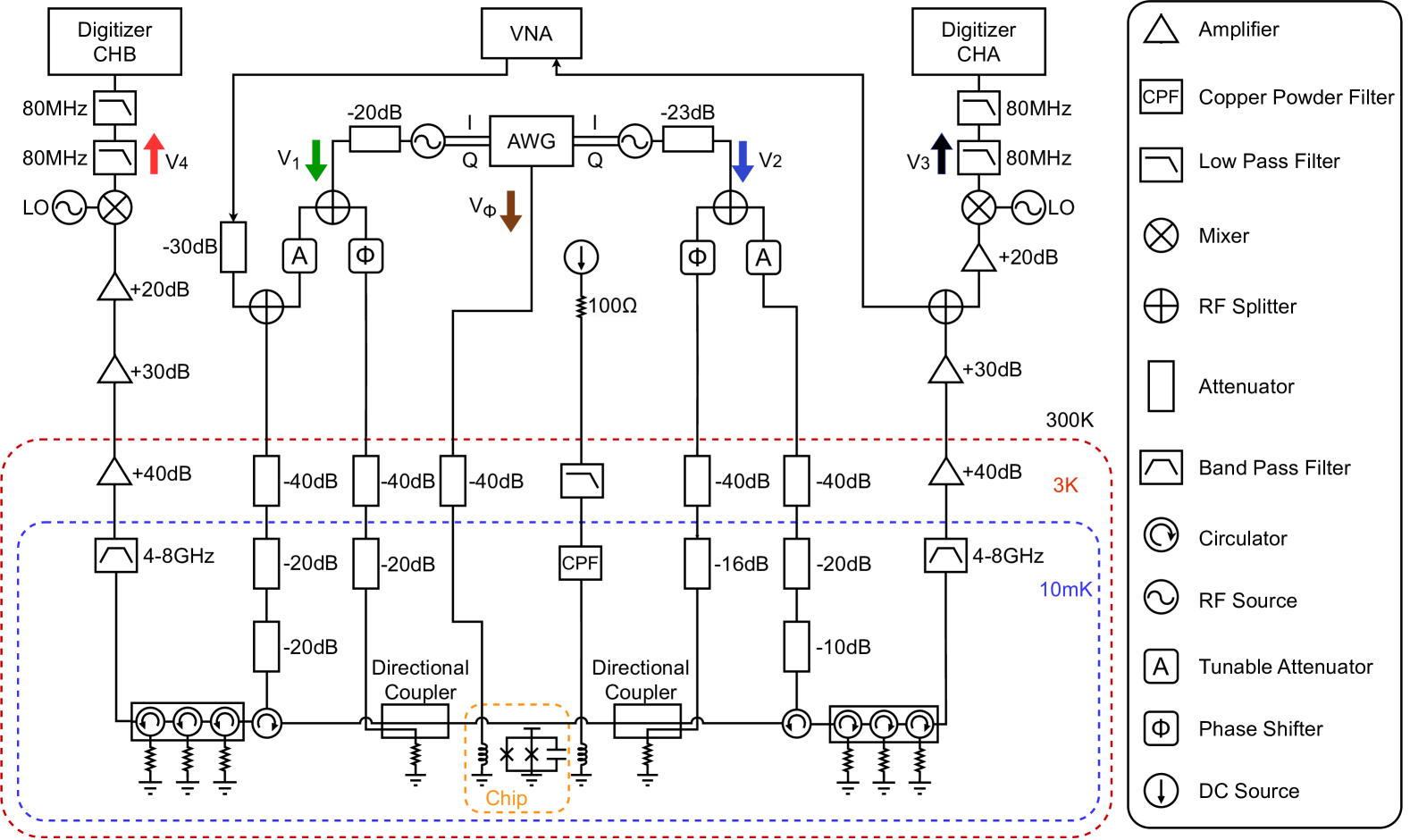
Figure S1: Schematic of the experimental setup. The superconducting artificial atom, a transmon qubit, is in the orange dashed box. The transmon is regulated by room-temperature electronics, including a flux line, input lines, and readout lines. The blue and red dashed boxes indicate different temperature stages within the dilution refrigerator.

The experimental setup, illustrated in Fig. S1, consists of a sample box containing a chip (highlighted by an orange dashed box) that features a single artificial atom capacitively coupled to an open one-dimensional transmission line. This assembly is mounted at the bottom of a dilution refrigerator operating at a base temperature of 10 mK. A superconducting magnetic coil, centrally positioned on the sample box, is used to tune the resonance frequency of the artificial atom. This coil is controlled by a DC source at room temperature, connected through a low-pass filter (LPF) and a copper powder filter (CPF) for noise filtering. The experimental setup is symmetrically arranged on both sides of the sample box to facilitate both frequency-domain and time-domain measurements, supporting our beam-splitter and beam-combiner experiments.

Single-tone spectroscopy is conducted using a vector network analyzer (VNA) to characterize the qubit, detailed further in Sec. S2. During these experiments, a weak probe field is introduced through the VNA at a probe frequency $\omega_{p}$, attenuated at several stages within the dilution refrigerator. A cryogenic circulator then directs this input field to interact with the qubit. The field transmitted from the qubit is captured by the VNA after passing through a series of cryogenic circulators, a band-pass filter (BPF), and a two-stage amplification process involving a high-electron-mobility transistor (HEMT) amplifier at 3 K and another amplifier at room temperature.

For time-domain measurements, an arbitrary waveform generator (AWG) generates IQ signals for the IQ modulator of the radio-frequency (RF) source to produce shaped modulation signals. The modulation signals are input as a pulse on the left side ($V_{1}$, green arrow), and/or a continuous wave on the right side ($V_{2}$, blue arrow). The output signals, $V_{3}$ (black arrow) and $V_{4}$ (red arrow), on both sides are measured at digitizer channels $A$ and $B$ (CHA and CHB), respectively. Additionally, an RF splitter is utilized at the input sides of the modulation signals. One of the split fields is routed to the cryogenic circulator through several attenuators and a tunable attenuator, denoted by A, at room temperature. The other field is connected to the directional coupler through several attenuators and a phase shifter, denoted as $\Phi$, at room temperature. This configuration mitigates leakage from the imperfect isolation of the circulators. The detailed procedure for cancellation of leakage fields can be found in Ref. Hoi et al. (2013a). The near-perfect cancellation of leakage field can be seen in Fig. 3 [$V_{3}$ ($V_{2,\text{in}}$ w/o qubit) and $V_{4}$ ($V_{1,\text{in}}$ w/o qubit)] in the main text. The local flux through the chip (inside the orange-dashed box) is controlled by the AWG via the $V_{\Phi}$ line (brown arrow) for fast switching, with a $-40\,\mathrm{dB}$ attenuation at 3 K.

S2 Single-tone spectroscopy in the frequency domain

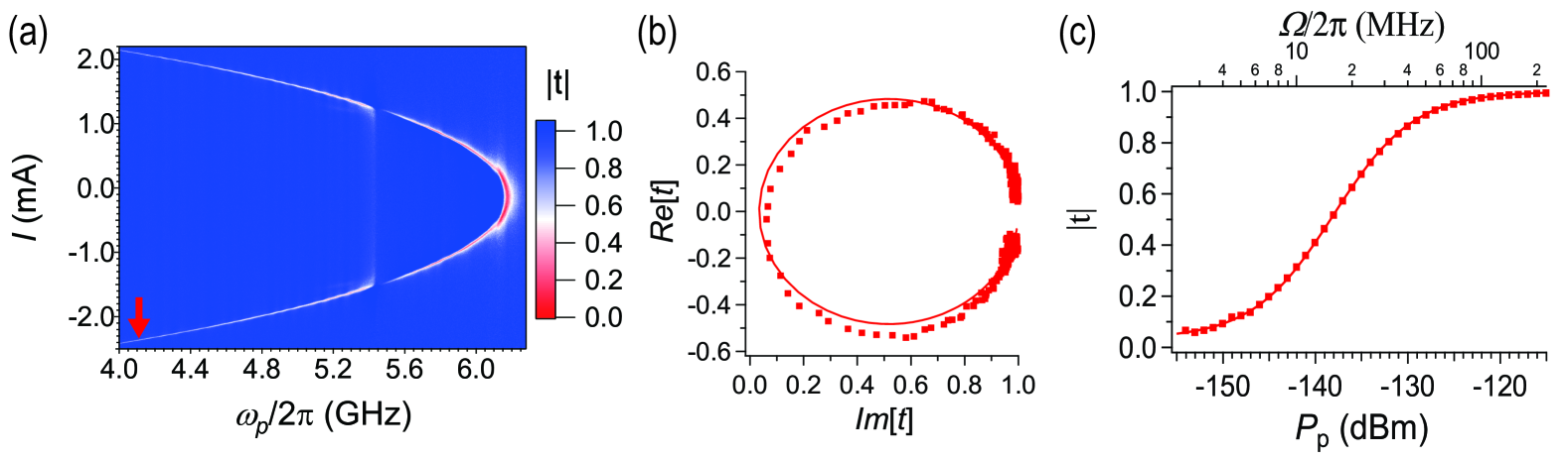
Figure S2: Single-tone frequency-domain measurement of the transmission coefficient. (a) Transmission coefficient as a function of probe frequency $\omega_{p}$ and the current $I$ controlling the flux through the SQUID of the transmon qubit. (b) Transmission coefficient plotted in the IQ plane for a weak probe (i.e., assuming $\Omega\ll\gamma$). (c) The on-resonance transmission magnitude $\left|t\right|$ as a function of probe power $P_{p}(\propto\Omega^{2})$. The solid curves in panels (a) and (b) are theory using Eqs. (4) and (5) in the main text.

To characterize the parameters of the qubit, we conducted single-tone spectroscopy. Fig. S2(a) illustrates the magnitude of the transmission coefficient, $\left|t\right|$, as a function of the probe frequency $\omega_{p}$ and the current $I$ applied in the superconducting coil to control the global flux that sets the transition frequencies of the transmon. The spectrum reveals the cosine dependence on the flux of the qubit’s $|0\rangle\leftrightarrow|1\rangle$ transition frequency. We note that a stray cavity resonance is visible at $\omega_{p}/2\pi=5.425\,\mathrm{GHz}$, accompanied by additional box modes appearing as vertical lines near the stray cavity and the apex. To avoid interference from these modes, we selected a biasing point for our beam-splitter and -combiner experiments at $\omega_{p}/2\pi=4.1108\,\mathrm{GHz}$, marked by a red arrow.

$E_{C}/h$	$E_{J}/h$	$E_{J}/E_{C}$	$\omega/2\pi$	$\Gamma/2\pi$	$\Gamma^{n}/2\pi$	$\gamma/2\pi$	$\phi$
[MHz]	[GHz]	-	[GHz]	[MHz]	[MHz]	[MHz]	[rad]
199.4	25.57	128.24	4.1108	22.15	0.39	11.47	0.0526

Table S1: Extracted qubit parameters. We obtain the resonance frequency $\omega$, the relaxation rate $\Gamma$, and the decoherence rate $\gamma$ from Fig. S2(b) by circle fitting in the IQ plane Probst et al. (2015); Lu et al. (2021). The non-radiative decay rate $\Gamma^{n}$ is calculated using $\gamma=\Gamma/2+\Gamma^{n}$. We extracted the anharmonicity between the $|0\rangle\leftrightarrow|1\rangle$ and $|1\rangle\leftrightarrow|2\rangle$ transitions from two-tone spectroscopy Hoi et al. (2013b). The anharmonicity approximately equals the charging energy $E_{C}$ Koch et al. (2007). $\phi$ is the mismatch angle due to the impedance mismatch from the transmission lines.

In Fig. S2(b), the transmission coefficient is depicted in the IQ plane for weak probe power $P_{p}$, where the Rabi frequency $\Omega$ is significantly smaller than the decoherence rate $\gamma$, resulting in a circular pattern. The experimental data points are indicated by red markers, while the solid curve represents the theoretical circle fit Probst et al. (2015); Lu et al. (2021), from which we extract the parameters $\omega$, $\Gamma$, and $\gamma$, all summarized in Table S1. Note that we have accounted for impedance mismatch $\phi$ in both the theoretical curve and the experimental data in Fig. S2(b)-(c).

Additionally, Fig. S2(c) displays the magnitude of the transmission coefficient, $\left|t\right|$, as a function of $P_{p}$ at the resonance frequency of the qubit. For low probe power, the incident coherent field undergoes extinction by up to 94.7 % in amplitude. With increasing probe power, a strong non-linearity emerges, saturating the qubit at high probe powers and leading to a unity transmission coefficient Hoi et al. (2011). The experimental data points are marked with red markers, and the theoretical fit is shown with a solid curve. All extracted parameters are summarized in Table S1.

S3 Calibration measurements in the time domain

To calibrate the gain and the attenuation of the input-output lines, we employ a time-domain setup as illustrated in Fig. S1 and perform single-tone calibration measurements. We bias our qubit at a resonance frequency of $\omega/2\pi=4.1108\,\mathrm{GHz}$ and apply a pulse with a duration of $2\,\mathrm{\mu s}$. This duration is chosen to ensure that the qubit reaches a steady state, enabling us to obtain the average on-resonance signal in the steady state, ${\left\langle V_{t,\text{on}}\right\rangle}$, across various probe powers. Similarly, we conduct experiments with the qubit significantly far detuned to measure the average off-resonance signal ${\left\langle V_{t,\text{off}}\right\rangle}$. The magnitude of the transmission coefficient $\left|t\right|$ is calculated as

$$\left|t\right|=\left|\frac{\left\langle V_{t,\text{on}}\right\rangle}{\left\langle V_{t,\text{off}}\right\rangle}\right|.$$ (S1)

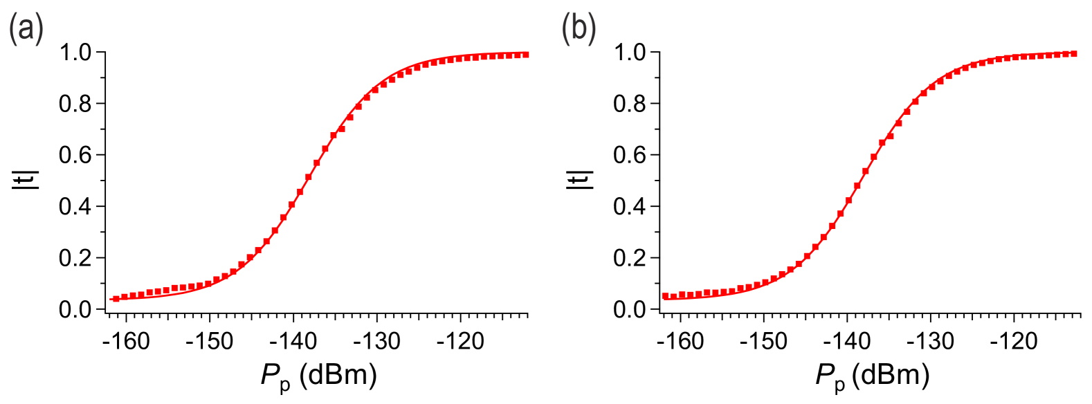
Figure S3: The magnitude of the transmission coefficient, $\left|t\right|$, as a function of probe power $P_{p}$ (converted from time domain) when the probe is resonant with the qubit. The figure displays both measured data points (markers) and theoretical fits (solid curves). (a) Measurements taken on digitizer channel $A$, with the input port located on the left side of the AWG, indicated by $V_{1}$ (green arrow) in Fig. S1. (b) Measurements taken on digitizer channel $B$, with the input port located on the right side of the AWG, indicated by $V_{2}$ (blue arrow) in Fig. S1.

Frequency domain		Time domain
$A_{\rm freq}$	$G_{\rm freq}$	$A_{\rm ChA}$	$G_{\rm ChA}$	$A_{\rm ChB}$	$G_{\rm ChB}$
$-125.05\,\mathrm{dB}$	69.13 dB	$-132.06\,\mathrm{dB}$	$89.77\,\mathrm{dB}$	$-132.82\,\mathrm{dB}$	$92.22\,\mathrm{dB}$

Table S2: Extracted gain $G$ and attenuation $A$ from frequency- and time-domain measurements Cheng et al. (2024). In the time-domain results, subscripts with ChA refer to calibration measurements taken on digitizer channel A with the input port for $V_{1}$, as shown in Fig. S3(a). Subscripts with ChB refer to measurements taken on digitizer channel B with the input port for $V_{2}$, as shown in Fig. S3(b).

Figure S3(a) presents measurement results across different probe powers, where the input port is connected to the left side of the AWG, as indicated by the green arrow, and the transmitted output is captured on digitizer channel $A$ in Fig. S1. Conversely, Fig. S3(b) features the input connected to the right side of the AWG, as indicated by the blue arrow in Fig. S1, with the transmitted output captured on digitizer channel $B$. The experimental data points are marked in red, while the solid curves represent theoretical fits using Eqs. (4) and (5) in the main text. Based on the method described in Ref. Cheng et al. (2024), we can determine the gain and attenuation in time-domain measurements. For frequency-domain measurements, using the same fitting method as in Fig. S2(c), we can also determine the gain and attenuation. All extracted gain and attenuation are summarized in Table S2.

S4 Calculation of the scattering matrix

In this section, we discuss the calculations for the elements of the scattering matrix. Initially, we detune the qubit far away, resulting in full transmission ($t=1$) for diagonal terms and no reflection ($r=0$) for off-diagonal terms. The scattering matrix can then be expressed as

$$\begin{pmatrix}V_{3}\\ V_{4}\end{pmatrix}=\begin{pmatrix}1&0\\ 0&1\end{pmatrix}\begin{pmatrix}V_{1}\\ 0\end{pmatrix}$$ (S2)

when the only input is the $V_{1}$ pulse ($V_{2}=0$). Here, $V_{3}=V_{1}$, as depicted in Fig. 1(a) of the main text. Similarly, we obtain $V_{4}=V_{2}$ when $V_{1}=0$:

$$\begin{pmatrix}V_{3}\\ V_{4}\end{pmatrix}=\begin{pmatrix}1&0\\ 0&1\end{pmatrix}\begin{pmatrix}0\\ V_{2}\end{pmatrix}.$$ (S3)

When the qubit interacts with the field, the scattering matrix includes $t_{L}$ and $t_{R}$ as diagonal terms, and $r_{L}$ and $r_{R}$ as off-diagonal terms. The subscripts “R" and “L" denote “right" and “left", respectively, referring to the direction relative to the sample. The scattering matrix becomes

$$\begin{pmatrix}V_{3}\\ V_{4}\end{pmatrix}=\begin{pmatrix}t_{L}&r_{R}\\ r_{L}&t_{R}\end{pmatrix}\begin{pmatrix}V_{1}\\ 0\end{pmatrix}.$$ (S4)

when only the $V_{1}$ pulse is used as input; we then obtain $V_{3}=t_{L}V_{1}$ and $V_{4}=r_{L}V_{1}$. Conversely, with $V_{1}=0$ and $V_{2}=V_{2}$, we find $V_{3}=r_{R}V_{2}$ and $V_{4}=t_{R}V_{2}$:

$$\begin{pmatrix}V_{3}\\ V_{4}\end{pmatrix}=\begin{pmatrix}t_{L}&r_{R}\\ r_{L}&t_{R}\end{pmatrix}\begin{pmatrix}0\\ V_{2}\end{pmatrix}$$ (S5)

Through these calculations, we derive the coefficients $r_{R}$, $t_{R}$, $r_{L}$, and $t_{L}$, representing the right reflection, right transmission, left reflection, and left transmission coefficients, respectively, within the scattering matrix. These parameters are summarized in Table II in the main text for Fig. 3(a). These coefficients provide valuable insights for evaluating the interference effects between the input pulses. Utilizing these coefficients, we simulate the theoretical results, allowing us to compare and validate experimental observations with theoretical predictions.

S5 Beam-splitter switching in the time domain

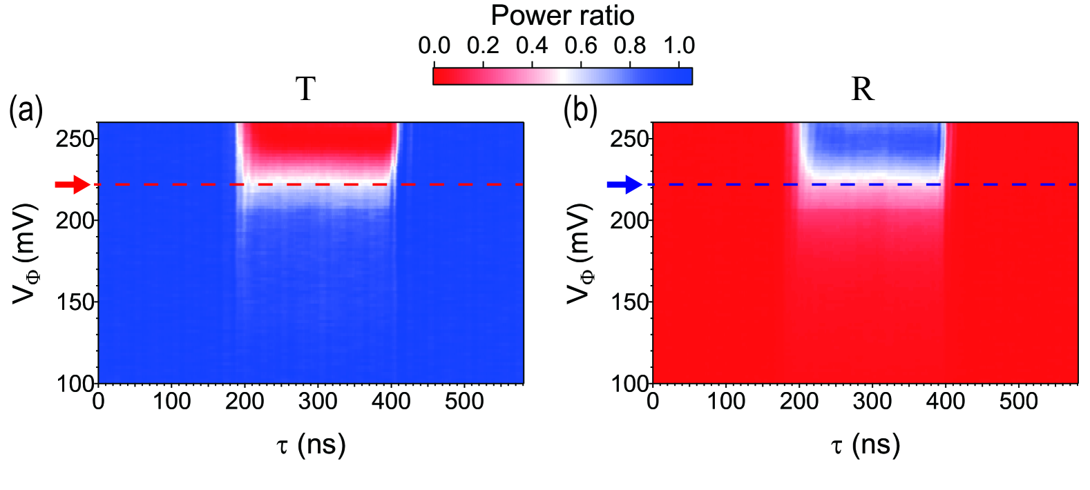
Figure S4: Power ratio (transmittance and reflectance) for the output signals as a function of time and of the flux-biasing amplitude $V_{\Phi}$ at weak probe power ($\Omega\ll\gamma$). (a) Transmittance $T$ measured using digitizer channel $A$. (b) Reflectance $R$ measured using digitizer channel $B$. A continuous wave is directed through one port of the open transmission line (indicated by a green arrow in Fig. S1) with a probe frequency $\omega_{p}/2\pi=4.1108\,\mathrm{GHz}$ at a weak probe power of $-158.98\,\mathrm{dBm}$. Simultaneously, a Gaussian pulse is applied to the local flux of the qubit (shown by the brown arrow in Fig. S1), with its voltage amplitude varying along the y axis, to adjust the qubit’s resonance frequency, changing T and R between zero and unity (top color bar). The dashed line marks the line cut used in the main text as Fig. 2(b).

In this section, we present the detailed results of Fig. 2(b) from the main text, shown in Fig. S4. First, we biased the qubit at $\omega/2\pi=4.2108\,\mathrm{GHz}$ (far detuned). Then, we varied the local flux by applying Gaussian pulses of varying amplitudes $V_{\Phi}$, as depicted on the y axis in Fig. S4. We continuously probed the system using a continuous wave at a frequency of $\omega_{p}/2\pi=4.1108\,\mathrm{GHz}$ with weak probe power. The pulse length is represented on the x axis.

In Fig. S4(a)-(b), a noticeable change in the power ratio (indicated by a shift in color) occurs as we sweep the amplitude of the local flux, which adjusts the $|0\rangle\leftrightarrow|1\rangle$ transition frequency of the qubit. Near 220 mV (indicated by a dashed line), we reach a 50:50 ratio (meaning that the system acts as a 50/50 beam splitter), similar to what is observed when the qubit is biased at $\omega/2\pi=4.12\,\mathrm{GHz}$ in Fig. 2(a) of the main text (highlighted by a purple arrow). As we further increase the amplitude of the local flux, the power ratio shifts towards 0 and 1, corresponding to the qubit being on resonance at $\omega/2\pi=4.1108\,\mathrm{GHz}$, with complementary values appearing in the lower region where the qubit is far detuned. This technique allows for switching the beam splitter in nanoseconds.

S6 Detailed data for the beam combiner around $T=0.5$

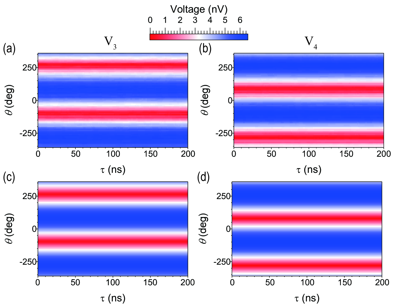
Figure S5: Beam-combiner results around $T=0.5$, as a function of time $\tau$ and the phase $\theta$ of the input $V_{1}$. (a) $V_{3}$ output signal measured using digitizer channel A. (b) $V_{4}$ output signal measured using digitizer channel B. (c, d) Theoretical simulations corresponding to panels (a) and (b), respectively, based on Eqs. (1)–(5) from the main text, using the parameters listed in Table II of the main text.

In this section, we present the detailed interference data of Fig. 3(a) in the main text. As mentioned, we set the qubit’s resonance frequency to $\omega/2\pi=4.12\,\mathrm{GHz}$ to achieve a transmittance and reflectance ratio of approximately 50:50. Two weak probes (labeled $V_{1}$ and $V_{2}$) at $\omega_{p}/2\pi=4.1108\,\mathrm{GHz}$ are simultaneously applied to the atom with phase $\theta$ for $V_{1}$. The output signals $V_{3}$ ($V_{4}$) are then measured using digitizer channel A (B), as shown in Fig. S5(a)-(b).

We extract and average the steady-state signal from the data corresponding to $\tau$ from 50 to 150 ns for each $\theta$ case. This yields the blue (red) data points in Fig. 3(a) in the main text. The experimental data matches well with the simulation results in Fig. S5(c)-(d).

References

- Hoi et al. (2013a) I.-C. Hoi, C. M. Wilson, G. Johansson, J. Lindkvist, B. Peropadre, T. Palomaki, and P. Delsing, “Microwave quantum optics with an artificial atom in one-dimensional open space,” New Journal of Physics 15, 025011 (2013a).
- Probst et al. (2015) S. Probst, F. B. Song, P. A. Bushev, A. V. Ustinov, and M. Weides, “Efficient and robust analysis of complex scattering data under noise in microwave resonators,” Review of Scientific Instruments 86, 024706 (2015).
- Lu et al. (2021) Y. Lu, A. Bengtsson, J. J. Burnett, E. Wiegand, B. Suri, P. Krantz, A. F. Roudsari, A. F. Kockum, S. Gasparinetti, G. Johansson, et al., “Characterizing decoherence rates of a superconducting qubit by direct microwave scattering,” npj Quantum Information 7, 35 (2021).
- Hoi et al. (2013b) I.-C. Hoi, C. Wilson, G. Johansson, J. Lindkvist, B. Peropadre, T. Palomaki, and P. Delsing, “Microwave quantum optics with an artificial atom in one-dimensional open space,” New Journal of Physics 15, 025011 (2013b).
- Koch et al. (2007) J. Koch, T. M. Yu, J. Gambetta, A. A. Houck, D. I. Schuster, J. Majer, A. Blais, M. H. Devoret, S. M. Girvin, and R. J. Schoelkopf, “Charge-insensitive qubit design derived from the Cooper pair box,” Physical Review A 76, 042319 (2007).
- Hoi et al. (2011) I.-C. Hoi, C. M. Wilson, G. Johansson, T. Palomaki, B. Peropadre, and P. Delsing, “Demonstration of a Single-Photon Router in the Microwave Regime,” Physical Review Letters 107, 073601 (2011).
- Cheng et al. (2024) Y.-T. Cheng, C.-H. Chien, K.-M. Hsieh, Y.-H. Huang, P. Y. Wen, W.-J. Lin, Y. Lu, F. Aziz, C.-P. Lee, K.-T. Lin, C.-Y. Chen, J. C. Chen, C.-S. Chuu, A. F. Kockum, G.-D. Lin, Y.-H. Lin, and I.-C. Hoi, “Tuning atom-field interaction via phase shaping,” Physical Review A 109, 023705 (2024).