Consistency Trajectory Matching for One-Step Generative Super-Resolution

Abstract

Current diffusion-based super-resolution (SR) approaches achieve commendable performance at the cost of high inference overhead. Therefore, distillation techniques are utilized to accelerate the multi-step teacher model into one-step student model. Nevertheless, these methods significantly raise training costs and constrain the performance of the student model by the teacher model. To overcome these tough challenges, we propose Consistency Trajectory Matching for Super-Resolution (CTMSR), a distillation-free strategy that is able to generate photo-realistic SR results in one step. Concretely, we first formulate a Probability Flow Ordinary Differential Equation (PF-ODE) trajectory to establish a deterministic mapping from low-resolution (LR) images with noise to high-resolution (HR) images. Then we apply the Consistency Training (CT) strategy to directly learn the mapping in one step, eliminating the necessity of pre-trained diffusion model. To further enhance the performance and better leverage the ground-truth during the training process, we aim to align the distribution of SR results more closely with that of the natural images. To this end, we propose to minimize the discrepancy between their respective PF-ODE trajectories from the LR image distribution by our meticulously designed Distribution Trajectory Matching (DTM) loss, resulting in improved realism of our recovered HR images. Comprehensive experimental results demonstrate that the proposed methods can attain comparable or even superior capabilities on both synthetic and real datasets while maintaining minimal inference latency.

1 Introduction

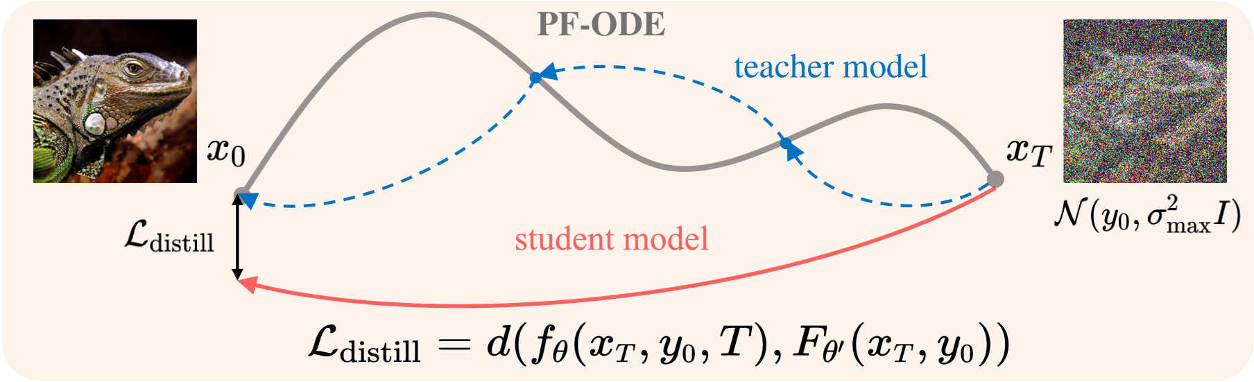
(a) Vanilla distillation. The student model ($f_{\theta}$) directly learns the PF-ODE from ${x}_{T}$ to ${x}_{0}$ formed by multi-step teacher model ($F_{\theta^{\prime}}$).

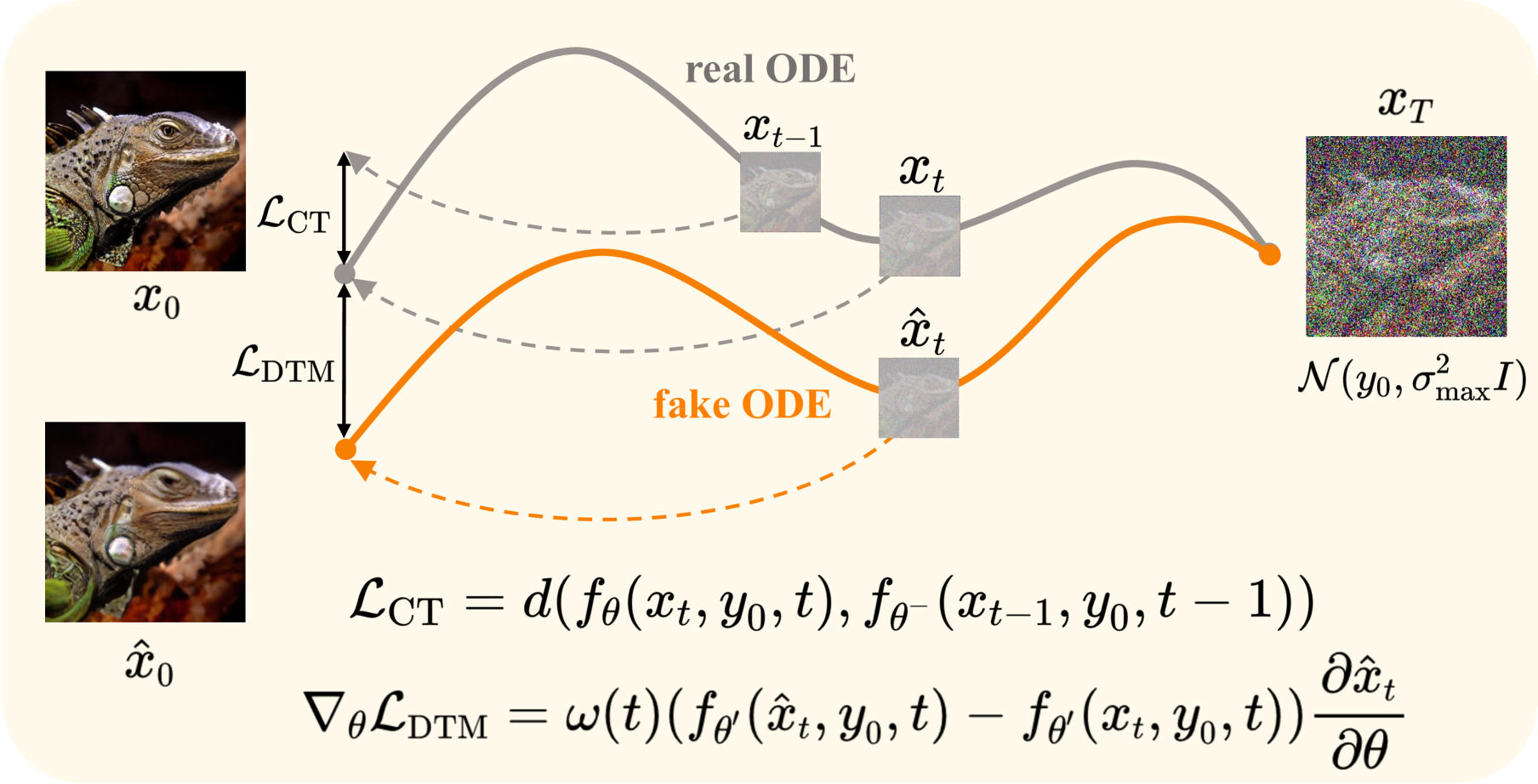
(b) Consistency Trajectory Matching for SR. We first utilize Consistency Training to map any point on the PF-ODE to the final point $x_{0}$ by minimizing the distance between model outputs of two adjacent points on the PF-ODE. Based on the learned ODE, we propose DTM to match the trajectory of fake ODE with the trajectory of real ODE, making the SR results better aligned with the distribution of natural images.

Figure 1: An illustrative comparison of vanilla distillation and our proposed Consistency Trajectory Matching for SR. In contrast to vanilla distillation, Consistency Training directly learns the deterministic mapping from noisy LR distribution to the natural image distribution to achieve one-step inference and DTM is proposed to further enhance the realism of SR results.

Single-image super-resolution (SISR) is a task of generating a high-resolution (HR) image that is in accordance with the input low-resolution (LR) image. As is known, SISR is a typical ill-posed problem in the field of low-level vision, since every LR image could consist with a number of potential HR counterparts. Early classical SR methods [47, 18, 31, 3] restore the HR images via optimizing the Root Mean Square Error (RMSE) loss function in a supervised manner. This methodology forces the model to learn an expectation of all possible HR counterparts, which leads to blurry SR results [15]. While generative SR methods aim to generate the HR estimation that conforms to the natural image distribution, thus producing more photo-realistic HR images. Recently, diffusion models [27, 11] have demonstrated strong capabilities in modeling complex distributions, e.g., the distribution of natural images, holding great potential for generative SR. Early diffusion-based SR works [25, 16, 33, 13] either condition the diffusion model on LR and train it as a common diffusion model (e.g., DDPM [11]), or leverage a pre-trained diffusion model as a prior and adjust the reverse process guided by LR images. Though these methods yield decent results, both of them require hundreds of inference steps. Therefore, numerous attempts have been made to accelerate the inference speed of diffusion-based SR models. While some studies [27, 20] investigated advanced inference strategies for reducing the sampling steps; [43, 21] propose to model the initial state of diffusion process as low-quality image perturbed by a slight amount of noise rather than pure noise, greatly reducing the inference steps for generative SR. Furthermore, SinSR [36] reformulates the inference process of ResShift [43] as Ordinary Differential Equation (ODE) and directly distills it into one step. However, as mentioned in [19], the performance of one-step student model is limited by the teacher model; if the ODE is not rectified to be straight during the training process of the teacher model, direct distillation could only produce sub-optimal results. Besides, distilling the teacher model involves multi-step sampling to generate training data pairs, which greatly increases the training overhead. Beyond these approaches, some Stable Diffusion-based methods [40, 39] leverage the powerful generative capabilities of pretrained Stable Diffusion (SD) and achieve impressive results in a single inference step. However, their reliance on a fixed backbone limits scalability to smaller models, restricting practical applicability. Therefore, how to obtain a distillation-free and backbone-independent one-step generative SR model that can produce photo-realistic SR results with limited inference footprint remains a challenging problem in the literature.

In order to tackle the aforementioned issues, we propose Consistency Trajectory Matching Super-Resolution (CTMSR), an efficient generative SR approach that could produce high-perceptual-quality HR images in merely one step. Instead of distilling one-step model from a pre-trained generative SR model, we leverage recent advances in Consistency Training (CT)  [30, 28] and directly learn a mapping function between LR images with noise to HR images. The proposed CT strategy enables us to directly learn a Probability Flow Ordinary Differential Equation (PF-ODE) trajectory, therefore eliminating the limitation of pre-trained multi-step diffusion model. Moreover, based on the learned PF-ODE trajectory, which is capable of transitioning noisy LR distribution to the natural image distribution, we propose the Distribution Trajectory Matching (DTM) loss to further improve our SR results. The proposed DTM loss penalizes the distribution discrepancy between our SR results and high quality images in a trajectory level by matching their respective PF-ODEs from the noisy LR distribution, resulting in improved perceptual quality of our SR results. Extensive experimental results on synthetic and real-world datasets clearly demonstrate the superiority of our methods. With less inference footprint, our proposed CTMSR is able to generate state-of-the-art photo-realistic SR results.

Our main contributions are summarized as follows:

• We propose the Consistency Training for SR to directly establish a PF-ODE from the noisy LR distribution to HR distribution. This enables us to produce photo-realistic SR results in one step without the need for distillation, achieving efficiency in both training and inference.

• Built upon the learned PF-ODE trajectory, we propose Distribution Trajectory Matching to better align the distribution of SR results with the distribution of natural images via trajectory matching, greatly enhancing realism.

• We provide comprehensive experimental results on both synthetic and real-world datasets. Compared with existing methods, our CTMSR achieves comparable or even better performance while maintaining less inference latency.

2 Related Work

2.1 Image Super-Resolution

Image super-resolution is a classical ill-posed problem that presents significant challenges in the field of low-level vision. Conventional SR methods [7, 9] recover the details of HR images via manually designing image priors guided by subjective knowledge. With the emergence of Deep Learning (DL), DL-based methods gradually dominate the realm of SR. Specifically, existing DL-based SR methods can be roughly categorized into two types: fidelity-oriented SR and generative SR. There exists numerous researches in fidelity-oriented SR [50, 6, 3, 17, 18, 47] that relies on minimization of the pixel distance (e.g., $\ell_{2}$ distance) between the reconstructed HR image and the ground-truth image in a supervised manner. Each of them makes efforts to improve the fidelity performance of SR from different aspects, varying from network architectures to loss functions and training strategies, and so on. Despite their success in achieving high Peak Signal-to-Noise Ratio (PSNR) scores, they inevitably produce over-smooth SR results. To overcome this challenge, generative SR methods [15, 34, 35] leverage the characteristic of generative models to model the distribution of natural images, aiming to optimize the SR model at the distribution level. Among them, diffusion-based techniques demonstrate exceptional performance in enhancing perceptual quality of SR results. Early diffusion-based SR methods [25, 16, 24] condition the diffusion model on LR images and train it the same way as a conventional diffusion model. Alternatively,  [33, 13, 4] utilize a pre-trained diffusion model as a prior and modify the reverse process based on LR images. Although these approaches yield satisfactory results, they generally require dozens or even hundreds of inference steps to generate HR images, since both methods start from an initial state of pure noise. To further enhance efficiency and tailor diffusion models more effectively for SR, ResShift [43] proposes modeling the initial state of the diffusion process as a LR image with a slight amount of noise rather than pure noise, thereby substantially reducing the required inference steps to 15. Additionally, SinSR [36] directly distills ResShift into single step. Although the distillation method has achieved substantial reductions in inference computational expense, limitations persist. It inevitably leads to considerable training costs and restricts the performance of the student model by the limitations of the teacher model.

2.2 Acceleration of Diffusion Models

Despite the strong generation capabilities manifested by diffusion models, considerable inference time overhead significantly hinders their practical application. Therefore, a range of acceleration techniques have been proposed to alleviate this issue. Certain approaches accomplish this by refining the inference process [27, 20, 49], while several methods [12, 22] concentrate on improving the diffusion schedule. Though these methods effectively reduce the inference steps to dozens, performance deteriorates markedly when the step count falls below ten. To overcome this limitation, distillation methods [42, 19, 26] are proposed to further compress the steps below ten while preserving promising performance. Among them, Progressive Distillation [26] effectively reduces the inference steps of student models through a multistage distillation. Nevertheless, the compounding errors at each distillation stage significantly undermine the overall performance of the student model. DMD [42] seeks to minimize the Kullback–Leibler (KL) divergence between the distribution of generated images and that of natural images by distilling the scores in pre-trained diffusion models, ultimately reducing the inference process to a single step. For SR task, the distillation approach has also been leveraged by SinSR [36] to distill ResShift [43] into one step. In addition, Consistency Model [30] is able to achieve promising results in 2${\sim}$4 steps, which is trained either by distillation or from scratch. Drawing inspiration from Consistency Model, we propose a distillation-free diffusion-based SR method with one-step inference in this paper.

3 Methodology

3.1 Preliminaries

Diffusion Models. Diffusion models are a type of generation model that transforms the distribution of natural images (i.e., $p_{\text{data}}(\bm{x})$) into a Gaussian noise distribution (i.e., $\mathcal{N}(0,\sigma_{\text{max}}^{2}\bm{I})$ through a forward process and constructs a reverse sampling process from pure noise to natural images. Specifically, the forward marginal distribution is defined as: $q(\bm{x}_{t}|\bm{x}_{0})=\mathcal{N}(\bm{x}_{t};\bm{x}_{0},\sigma(t)^{2}\bm{I})$, where $\sigma(t)$ is a predefined function that controls the schedule of noise and obeys $\sigma(0)=0$ and $\sigma(T)=\sigma_{\text{max}}$. To simplify the representation of $\bm{x}_{t}$, the forward marginal distribution can be reparameterized as:

$$\begin{split}\bm{x}_{t}=\bm{x}_{0}\ +\ \sigma(t)\bm{\epsilon},\quad\mathrm{where}\ \bm{\epsilon}\sim\mathcal{N}(\bm{0},\bm{I}).\end{split}$$ (1)

According to [12, 29], the forward process could be represented in the form of Stochastic Differential Equation (SDE):

$$\mathrm{d}\bm{x}=\dot{\sigma}(t)\ \mathrm{d}\omega_{t},$$ (2)

where the dot denotes a time derivative and $\omega_{t}$ is the standard Wiener process. Correspondingly, an ordinary differential equation (ODE) can be employed to represent the reverse solution of this forward SDE, called the Probability Flow ODE (PF-ODE) [29, 20]:

$$\mathrm{d}\bm{x}=\dot{\sigma}(t)\ \bm{\epsilon}_{\bm{\theta}}(\bm{x}_{t},\bm{y}_{0},t)\ \mathrm{d}t,$$ (3)

where $\bm{\epsilon}_{\bm{\theta}}(\bm{x}_{t},\bm{y}_{0},t)$ is reparameterized by a neural network with parameter $\bm{\theta}$, aiming at predicting $\bm{\epsilon}$.

Consistency Training. With the PF-ODE formulated as Eq. 3, the Consistency Model [30] (CM) directly estimates the solution of the PF-ODE, thus allowing for one-step generation:

$$\bm{f}_{\bm{\theta}}(\bm{x}_{T},T)\approx\bm{x}_{0}=\bm{x}_{T}+\int_{T}^{0}\frac{\mathrm{d}\bm{x}_{s}}{\mathrm{d}s}\mathrm{d}s.$$ (4)

Specifically, Consistency Training (CT) is proposed to train a CM that eliminates the need of pre-trained diffusion model. It first samples two adjacent points along the ODE trajectory and then minimizes the difference between model outputs corresponding to these two points. Then the training objective

$$\mathcal{L}(\bm{\theta},\bm{\theta}^{-})=\mathbb{E}_{\bm{x},t}[d\left(f_{\bm{\theta}}(\bm{x}_{t},t),\bm{f}_{\bm{\theta}^{-}}(\bm{x}_{t-1},t-1)\right)]$$ (5)

is adopted to optimize the online model $\bm{\theta}$ to approximate the target model, where $d(\cdot,\cdot)$ denotes a predefined metric function for measuring the distance between two samples and $\bm{\theta}^{-}$ is obtained by exponential moving average (EMA) of the parameter $\bm{\theta}$, i.e., $\bm{\theta}^{-}\leftarrow\mu\bm{\theta}^{-}\ +\ (1-\mu)\bm{\theta}$.

Figure 2: The pipeline of the proposed CTMSR. We first employ CT loss to train our CTMSR until convergence to get a pre-trained CTMSR ($f_{\theta^{\prime}}$) with parameters frozen. As our pre-trained CTMSR is able to construct the PF-ODE trajectory from one distribution to another, we feed $\hat{x}_{t^{\prime}}$ and $x_{t^{\prime}}$ into the pre-trained CTMSR to get the trajectories of fake ODE and real ODE respectively, namely $x_{\text{fake}}$ and $x_{\text{real}}$. Then we calculate the $\nabla_{\theta}\mathcal{L}_{\mathrm{DTM}}$ that matches the trajectories to penalize the distribution discrepancy between our SR results and the real images in a trajectory level. With the calculated $\nabla_{\theta}\mathcal{L}_{\mathrm{DTM}}$ backpropagated to our training CTMSR, the realism of SR results produced by our model will be further enhanced.

Score Distillation. Score distillation methods [23, 38] are proposed for training a 3D generator with pre-trained image diffusion models. Specifically, by perturbing the rendered image $\hat{z}$ with noise $\bm{\epsilon}$, the seminal work of score distillation sampling (SDS) [23] is able to penalize the discrepancy between rendered images and the distribution captured by pre-trained diffusion model:

$$\nabla_{\theta}\mathcal{L}_{\mathrm{SDS}}(\hat{\bm{z}},t,\bm{\epsilon})=\left(\bm{\epsilon}_{\bm{\phi}}(\hat{\bm{z}}_{t},t)-\bm{\epsilon}\right)\frac{\partial\hat{\bm{z}}_{t}}{\partial\bm{\theta}},$$ (6)

where $\hat{\bm{z}}_{t}$ refers to the noised version of $\hat{\bm{z}}$, $\bm{\epsilon}_{\bm{\phi}}(\cdot)$ is the pretrained diffusion model and $\bm{\theta}$ denotes the generator parameter . More details about score distillation methods can be found in [23, 38, 10]. In this paper, the above idea of score distillation inspires us to align the distribution of generated images, i.e. SR outputs, with natural images through trajectory matching. Since our CT could construct a PF-ODE trajectory between noisy LR images and high quality images, we are able to optimize the distribution discrepancy between our SR results and high quality images by matching their respective PF-ODEs from the noisy LR distribution.

3.2 Consistency Trajectory Matching for SR

Current diffusion-based SR models typically rely on multi-step inference, which incurs significant time overhead. Although distillation techniques have been employed to reduce the inference steps to a single step, they still suffer from high training costs and the performance limitations imposed by the teacher model. To address these issues, we first introduce the application of CT strategy into SR model to achieve one-step inference in a distillation-free manner in Sec. 3.2.1. Besides, to better align the SR results with the natural image distribution, we propose Distribution Trajectory Matching in Sec. 3.2.2 to match their respective PF-ODE trajectories from the LR image distribution.

3.2.1 Consistency Training for SR

To better leverage the prior information from LR images, we formulate the forward process tailored for SR task [43] based on Eq. 1 :

$$\begin{split}\bm{x}_{t}=\bm{x}_{0}\ +\ \alpha(t)\bm{e}_{0}+\sigma(t)\bm{\epsilon},\quad\mathrm{where}\ \bm{\epsilon}\thicksim\mathcal{N}(\bm{0},\bm{I}),\end{split}$$ (7)

where $\alpha(t)$ is a predefined function that controls the schedule of residual and obeys $\alpha(0)=0$ and $\alpha(T)=1$. Based on Eq. 3, we formulate the PF-ODE as:

$$\mathrm{d}\bm{x}=[\dot{\alpha}(t)\ \bm{e}_{\bm{\theta}}(\bm{x}_{t},\bm{y}_{0},t)\ +\ \dot{\sigma}(t)\ \bm{\epsilon}_{\bm{\theta}}(\bm{x}_{t},\bm{y}_{0},t)]\ \mathrm{d}t,$$ (8)

where $\bm{e}_{\bm{\theta}}(\bm{x}_{t},\bm{y}_{0},t)$ is reparameterized by a neural network with parameter $\bm{\theta}$ that aims at predicting $\bm{e}_{0}$. As described in Eq. 8, HR images can be restored from LR images by solving the PF-ODE from $T$ to 0. Then we introduce the consistency model $\bm{f}_{\bm{\theta}}(\bm{x}_{t},t)\rightarrow\bm{x}_{0}$ to map any point on the PF-ODE to the final solution for $t=0$. We parameterize the $\bm{f}_{\bm{\theta}}$ as follows:

$$\bm{f}_{\bm{\theta}}(\bm{x}_{t},\bm{y}_{0},t)=c_{\text{skip}}(t)\bm{x}_{t}\ +\ c_{\text{out}}(t)\bm{F}_{\bm{\theta}}(\bm{x}_{t},\bm{y}_{0},t),$$ (9)

where $c_{\text{skip}}(t)$ and $c_{\text{out}}(t)$ are predefined to satisfy $c_{\text{skip}}(0)=1,c_{\text{out}}(0)=0$ and $\bm{F}_{\bm{\theta}}$ is the actual neural network parameterized by $\bm{\theta}$. We then discretize the trajectory into $T$ intervals, with boundaries $0,1,\ldots,T$, namely $T+1$ points on the PF-ODE trajectory. During training, we randomly select two adjacent points on the trajectory (i.e., $x_{t-1},x_{t}$) and minimize their consistency loss $\mathcal{L}_{\text{CT}}$ as:

$$\mathbb{E}_{\bm{x},n}[d(f_{\bm{\theta}}(\bm{x}_{t},\bm{y}_{0},t),\bm{f}_{\bm{\theta}^{-}}(\bm{x}_{t-1},\bm{y}_{0},t-1))],$$ (10)

where $\bm{\theta}^{-}\leftarrow\text{stopgrad}(\bm{\theta})$ according to [28]. Equipped with CT strategy, our method could reconstruct the HR images through the learned PF-ODE trajectory in single-step inference. To simplify the representation, we denote $f_{\bm{\theta}}(\bm{x}_{t},\bm{y}_{0},t)$ as $\bm{x}_{\text{est}}$ and $\bm{f}_{\bm{\theta}^{-}}(\bm{x}_{t-1},\bm{y}_{0},t-1)$ as $\bm{x}_{\text{tar}}$, since $\bm{x}_{\text{est}}$ is the estimation of target $\bm{x}_{\text{tar}}$.

3.2.2 Distribution Trajectory Matching

Although utilizing training strategy of CT could already yield promising results in one-step inference, limitations persist. We observe that information contained in ground-truth is not effectively utilize during training, as only the point closest to $\bm{x}_{0}$ (i.e., $\bm{x}_{1}$) could directly participate in the calculation of the consistency loss with $\bm{x}_{0}$, while other points could only leverage $\bm{x}_{0}$ in a mediated way by calculating the consistency loss with the neighbouring points. Moreover, since our SR model pre-trained with $\mathcal{L}_{\text{CT}}$ is capable of estimating the PF-ODE trajectory from one distribution to another, it offers a means to optimize SR model at the distribution level. Based on these observations, we propose Distribution Trajectory Matching (DTM), a trajectory-based loss function by which we could optimize our SR model to bring the SR results closer to the natural image distribution.

Firstly, we estimate the PF-ODE trajectory to the distribution of natural images, namely the real ODE:

$$\bm{f}_{\bm{\theta}^{\prime}}(\bm{x}_{t},\bm{y}_{0},t)=\bm{x}_{t}+\int_{t}^{0}\frac{\mathrm{d}\bm{x}_{s}}{\mathrm{d}s}\mathrm{d}s,\vskip-5.69054pt$$ (11)

where

$$\begin{split}\frac{\mathrm{d}\bm{x}_{s}}{\mathrm{d}s}&=\dot{\alpha}(s)\bm{e}_{\bm{\theta}^{\prime}}(\bm{x}_{s},\bm{y}_{0},s)\ +\ \dot{\sigma}(s)\bm{\epsilon}_{\bm{\theta}^{\prime}}(\bm{x}_{s},\bm{y}_{0},s)\\ &=d_{\bm{\theta}^{\prime}}(\bm{x}_{s},\bm{y}_{0},s),\end{split}\vskip-5.69054pt$$ (12)

$\bm{\theta}^{\prime}$ denotes the parameters of pre-trained CTMSR. In contrast to the real ODE, we regard the SR results produced by our model as the fake distribution and construct a fake ODE as:

$$\bm{f}_{\bm{\theta}^{\prime}}(\hat{\bm{x}}_{t},\bm{y}_{0},t)=\hat{\bm{x}}_{t}+\int_{t}^{0}d_{\bm{\theta}^{\prime}}(\hat{\bm{x}}_{s},\bm{y}_{0},s)\mathrm{d}s.$$ (13)

Here, $\hat{\bm{x}}_{t}$ shares the same forward process of ${\bm{x}}_{t}$:

$$\hat{\bm{x}}_{t}=\hat{\bm{x}}_{0}\ +\ \alpha(t)\hat{\bm{e}}_{0}+\sigma(t)\bm{\epsilon},$$ (14)

where $\bm{\epsilon}\sim\mathcal{N}(\bm{0},\bm{I})$ , $\hat{\bm{x}}_{0}$ is the output of the SR model (i.e., $\hat{\bm{x}}_{0}=\bm{f}_{\bm{\theta}}(\hat{\bm{x}}_{t^{\prime}},\bm{y}_{0},t^{\prime})$) and $\hat{\bm{e}}_{0}=\bm{y}_{0}-\hat{\bm{x}}_{0}$.

To bring the fake distribution closer to the real distribution, we propose to align the trajectory from $\hat{\bm{x}}_{t}$ to the fake distribution with the trajectory from $\bm{x}_{t}$ to the real distribution as illustrated in Figure 1(b). To be specific, we expect to minimize the Distribution Trajectory Distance (DTD) between $\bm{f}_{\bm{\theta}^{\prime}}(\bm{x}_{t},\bm{y}_{0},t)$ and $\bm{f}_{\bm{\theta}^{\prime}}(\hat{\bm{x}}_{t},\bm{y}_{0},t)$, with the corresponding loss function as follows:

$$\mathcal{L}_{\mathrm{DTD}}=\mathbb{E}_{\bm{x},t}\left\|\omega(t)[\bm{f}_{\bm{\theta}^{\prime}}(\hat{\bm{x}}_{t},\bm{y}_{0},t)-\bm{f}_{\bm{\theta}^{\prime}}(\bm{x}_{t},\bm{y}_{0},t)]\right\|_{2}^{2},$$ (15)

where $\omega(t)$ is a weighting function that depends on $t$. We can further expand this equation into the following form based on Eq. 11, 12, 13:

$$\begin{split}\mathcal{L}_{\mathrm{DTD}}&=\mathbb{E}_{\bm{x},t}\|\omega(t)[(\hat{\bm{x}}_{t}-\bm{x}_{t})+\\ &(\int_{t}^{0}[d_{\bm{\theta}^{\prime}}(\hat{\bm{x}}_{s},\bm{y}_{0},s)-d_{\bm{\theta}^{\prime}}({\bm{x}}_{s},\bm{y}_{0},s)]\mathrm{d}s)]\|_{2}^{2},\end{split}$$ (16)

where $t\in[T_{\text{min}},T_{\text{max}}]$. In Eq. 16, the first term represents sampling points at time $t$ along both trajectories and minimizing the distance between them; the second term ensures that the directions of all subsequent points on the two paths, before time $t$, remain consistent, which implicitly minimizes the distance between these points. Therefore, we could match these two trajectories from time $t$ to 0 by minimizing $\mathcal{L}_{\mathrm{DTD}}$, resulting in a better alignment between the SR results and natural images at the distribution level. Inspired by [23, 38], we minimize the $\mathcal{L}_{\mathrm{DTD}}$ to eventually get $\bm{\theta}^{*}=\arg\min_{\bm{\theta}}\mathcal{L}_{\mathrm{DTD}}$ by exclusively updating $\bm{\theta}$ while keeping $\bm{\theta}^{\prime}$ fixed. And the gradient of $\mathcal{L}_{\mathrm{DTD}}$ with respect to the parameters $\bm{\theta}$, $\nabla_{\bm{\theta}}\mathcal{L}_{\mathrm{DTD}}$, is given by:

$$\omega(t)\left(\bm{f}_{\bm{\theta}^{\prime}}(\hat{\bm{x}}_{t},\bm{y}_{0},t)-\bm{f}_{\bm{\theta}^{\prime}}(\bm{x}_{t},\bm{y}_{0},t)\right)\frac{\partial\bm{f}_{\bm{\theta}^{\prime}}(\hat{\bm{x}}_{t},\bm{y}_{0},t)}{\partial\hat{\bm{x}}_{t}}\frac{\partial\hat{\bm{x}}_{t}}{\partial\theta}.\vskip 8.53581pt$$ (17)

Algorithm 1 Overall training procedure of CTMSR.

0: training CTMSR $\bm{f}_{\bm{\theta}}(\cdot)$

0: Paired training dataset $(X,Y)$

1: Stage 1: Consistency Training for One-Step SR

2: $k\leftarrow 0$

3: while not converged do

4:  $\bm{\theta}^{-}\leftarrow\text{stopgrad}(\bm{\theta})$

5:  sample $\bm{x}_{0},\bm{y}_{0}\sim(X,Y)$

6:  sample $t\sim U(1,T(k))$

7:  compute $\bm{x}_{t},\bm{x}_{t+1}$ using Eq. 1

8:  $\mathcal{L}_{\text{CT}}=d(\bm{f}_{\bm{\theta}}(\bm{x}_{t},\bm{y}_{0},t),\bm{f}_{\bm{\theta}^{-}}(\bm{x}_{t-1},\bm{y}_{0},t-1))$

9:  Take a gradient descent step on $\nabla_{\theta}\mathcal{L}_{\text{CT}}$

10:  $k\leftarrow k+1$

11: end while

12: Stage 2: Distribution Trajectory Matching

13: $\bm{\theta}^{\prime}\leftarrow\text{stopgrad}(\bm{\theta})$

14: while not converged do

15:  sample $\bm{x}_{0},\bm{y}_{0}\sim(X,Y)$

16:  sample $t^{\prime}\sim U(1,T(k))$

17:  compute $\bm{x}_{t^{\prime}}$ using Eq. 1

18:  $\hat{\bm{x}}_{0}=\bm{f}_{\bm{\theta}}(\bm{x}_{t^{\prime}},\bm{y}_{0},t^{\prime})$

19:  sample $t\sim U(T_{\text{min}},T_{\text{max}})$

20:  compute $\bm{x}_{t},\hat{\bm{x}}_{t}$ using Eq. 1

21:  $\nabla_{\theta}\mathcal{L}_{\mathrm{DTM}}=\left(\bm{f}_{\bm{\theta}^{\prime}}(\hat{\bm{x}}_{t},\bm{y}_{0},t)-\bm{f}_{\bm{\theta}^{\prime}}(\bm{x}_{t},\bm{y}_{0},t)\right)\frac{\partial\hat{\bm{x}}_{t}}{\partial\theta}$

22:  Take a gradient descent step on $\nabla_{\theta}\mathcal{L}_{\text{CT}}+\nabla_{\theta}\mathcal{L}_{\text{DTM}}$

23:  $k\leftarrow k+1$

24: end while

25: return  Converged CTMSR $f_{\theta}(\cdot)$.

Methods	Metrics
8
	PSNR$\uparrow$	SSIM$\uparrow$	LPIPS$\downarrow$	CLIPIQA$\uparrow$	MUSIQ$\uparrow$	MANIQA$\uparrow$	NIQE$\downarrow$
ESRGAN [34]	20.67	0.448	0.485	0.451	43.615	0.3212	8.33
BSRGAN [45]	24.42	0.659	0.259	0.581	54.697	0.3865	6.08
SwinIR [18]	23.99	0.667	0.238	0.564	53.790	0.3882	5.89
RealESRGAN [35]	24.04	0.665	0.254	0.523	52.538	0.3689	6.07
StableSR-200 [33]	22.19	0.574	0.318	0.580	49.885	0.3684	7.10
LDM-15 [24]	24.85	0.668	0.269	0.510	46.639	0.3305	7.21
ResShift-15 [43]	24.94	0.674	0.237	0.586	53.182	0.4191	6.88
ResShift-4 [43]	25.02	0.683	0.208	0.600	52.019	0.3885	7.34
SinSR-1 [36]	24.70	0.663	0.218	0.611	53.632	0.4161	6.29
CTMSR-1 (ours)	24.73	0.666	0.197	0.691	60.142	0.4859	5.66

Table 1: Quantitative results of models on ImageNet-Test. The best and second best results are highlighted in bold and underline. (”-N” behind the method name represents the number of inference steps)

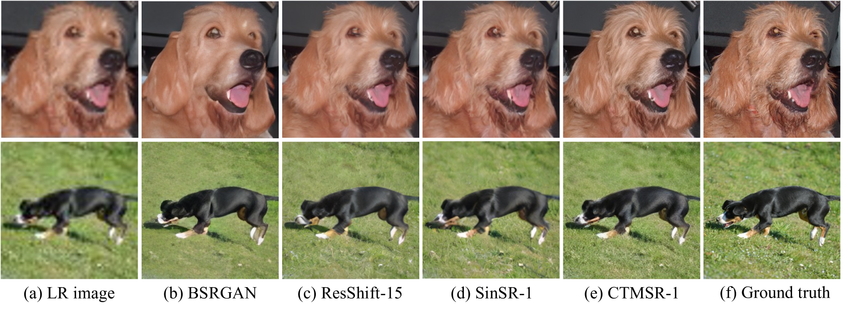
Figure 3: Visual comparisons of different methods on two synthetic examples of the ImageNet-Test dataset.

In practice, calculating the U-Net Jacobian term is computationally expensive, as it involves backpropagating through the U-Net of our model. Recent studies [23, 38] have shown that neglecting the Jacobian term leads to more effective gradient for optimization. Inspired by this observation, we omit the differentiation through the pre-trained SR model to obtain the Distribution Trajectory Matching (DTM),

$$\nabla_{\theta}\mathcal{L}_{\mathrm{DTM}}=\omega(t)\left(\bm{f}_{\bm{\theta}^{\prime}}(\hat{\bm{x}}_{t},\bm{y}_{0},t)-\bm{f}_{\bm{\theta}^{\prime}}(\bm{x}_{t},\bm{y}_{0},t)\right)\frac{\partial\hat{\bm{x}}_{t}}{\partial\theta}.$$ (18)

In practice, we formulate $\omega(t)$ as :

$$\omega(t)=\frac{CS}{\|\hat{\bm{x}}_{0}-\bm{x}_{0}\|_{1}},$$ (19)

where $S$ is the number of spatial locations and $C$ is the number of channels. The above DTM further improves the performance of our CTMSR by matching the trajectories of real ODE and fake ODE. We validate the effectiveness of DTM in ablation study in Sec. 4.3. The overall of our methods is summarized in Algorithm 2.

Methods	RealSR				RealSet65
9
	CLIPIQA$\uparrow$	MUSIQ$\uparrow$	MANIQA $\uparrow$	NIQE$\downarrow$	CLIPIQA$\uparrow$	MUSIQ$\uparrow$	MANIQA $\uparrow$	NIQE$\downarrow$
StableSR-200 [33]	0.4124	48.346	0.3021	5.87	0.4488	48.740	0.3097	5.75
LDM-15 [24]	0.3748	48.698	0.2655	6.22	0.4313	48.602	0.2693	6.47
ResShift-15 [43]	0.5709	57.769	0.3691	5.93	0.6309	59.319	0.3916	5.96
ResShift-4 [43]	0.5646	55.189	0.3337	6.93	0.6188	58.516	0.3526	6.46
SinSR-1 [36]	0.6627	59.344	0.4058	6.26	0.7164	62.751	0.4358	5.94
CTMSR-1 (ours)	0.6449	64.796	0.4157	4.65	0.6893	67.173	0.4360	4.51

Table 2: Quantitative results of models on two real-world datasets. The best and second best results are highlighted in bold and underline.

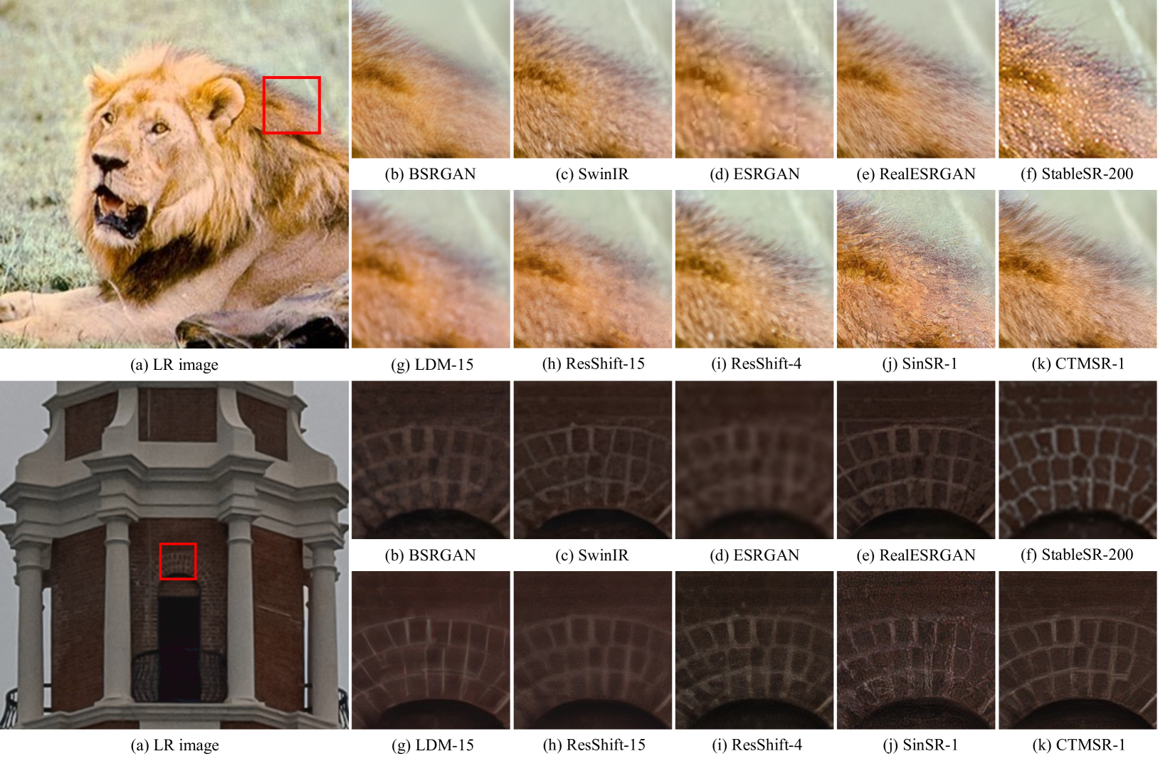
Figure 4: Visual comparisons of different methods on two examples of real-world datasets. Please zoom in for more details.

3.3 Implementation details

Network architectures. Analogous to ResShift [43], we adopt the UNet structure with Swin Transformer [44] block for our CTMSR. While as our Consistency Training for SR and Distribution Trajectory Matching techniques could effectively capture the transition from noisy LR distribution to the natural image distribution, we do not need to rely on the encoder and decoder of pre-trained VQ-GAN model [8] as in [43]. For the pursuit of efficient generative SR, we adopt tailored architecture for SR with pixel unshuffle operation and nearest neighbor upsampling, training all the parameters in the network from scratch. More details about our network architecture can be found in the supplementary file.

Metric function. As for metric function, we adopt widely used Learned Perceptual Image Patch Similarity (LPIPS, [48]) and Charbonnier [2] metrics. In practice, we configure the metric function as the weighted combination of these two metrics for optimal performance:

$$d(x,y)=\lambda_{1}\cdot\text{LPIPS}(x,y)+\lambda_{2}\cdot\text{Charbonnier}(x,y).$$ (20)

In practice, we set $\lambda_{1}=0.5$ and $\lambda_{2}=0.5$. More implementation details are included in the supplementary materials.

4 Experiments

4.1 Experimental Settings

Training details. Following [43, 24], we randomly crop $256\times 256$ patches from the training set of ImageNet [5] as our HR training data. LR images are synthesized using the degradation pipeline of RealESRGAN [35]. In the process of training, we first train our model with CT strategy for 500K iterations with fixed learning rate of 5e-5 and batch-size of 32. Then, we freeze the pre-trained model as $\bm{f}_{\bm{\theta}^{\prime}}$ and further optimize $\bm{f}_{\bm{\theta}}$ with $\mathcal{L}_{\mathrm{DTM}}$ and $\mathcal{L}_{\mathrm{CT}}$ for another 10K iterations with learning rate of 5e-5.

Testing details. We utilize the dataset ImageNet-Test that includes 3,000 paired images randomly selected from the validation set of ImageNet [5] as our main dataset following the setting in [43]. Additionally, we adopt two real-world datasets, RealSR [1] and RealSet65 [43], to evaluate the generalizability of our model on real-world data. To comprehensively evaluate the performance of various methods, we utilize a series of full-reference and non-reference metrics. As for full-reference metrics, PSNR and SSIM [37] are used to measure the fidelity, while LPIPS [48], is used to measure the perceptual quality. PSNR and SSIM are evaluated on the Y channel in the YCbCr color space. The non-reference metrics consist of NIQE [46], CLIPIQA  [32], MANIQA [41] and MUSIQ [14]. NIQE assesses image quality by analyzing statistical features. MUSIQ utilizes Transformers to capture multi-scale distortions. MANIQA incorporates attention mechanisms for quality evaluation, and CLIPIQA leverages pre-trained models, such as CLIP, to align quality assessments with human perception.

4.2 Experimental Results

Evaluation on testing datasets. To demonstrate the superiority of our approach, we compare our approach with several representative SR methods, including diffusion-based methods and GAN-based methods. The diffusion-based methods incorporate StableSR [33], LDM [24], ResShift [43] and SinSR [36]. Other prominent GAN-based methods encompass ESRGAN [34], BSRGAN [45], SwinIR [18], RealESRGAN [35]. All the test results of the compared methods are evaluated based on their released codes and pre-trained model weights. The quantitative comparisons among various approaches are presented in Table 1 and Table 2. We can observe that our method achieves either the best or second-best performance on the perceptual quality metrics across all datasets. Specifically, on the synthetic dataset, CTMSR achieves the best performance on both reference-based and non-reference perceptual quality metrics, with only slightly lower scores on fidelity metrics PSNR and SSIM. As for real-world datasets, CTMSR achieves either the best or comparable performance across the non-reference metrics. Notably, in terms of MUSIQ, our method outperforms SinSR by 5.452 and 4.422 on the RealSR and RealSet datasets, respectively. Figure 3 and 4 illustrate some visual comparisons on synthetic datasets and real-world datasets, where it can be observed that our method generates more detailed and realistic textures without noticeable artifacts.

Methods	Runtime	LPIPS$\downarrow$	MUSIQ$\uparrow$	CLIPIQA$\uparrow$
StableSR-200	12889	0.3184	49.885	0.5801
LDM-15	223	0.2685	46.639	0.5095
ResShift-15	689	0.2371	53.182	0.5860
ResShift-4	210	0.2075	52.019	0.6003
SinSR-1	65	0.2183	53.632	0.6113
CTMSR-1	48	0.1969	60.142	0.6913

Table 3: Computational efficiency and performance comparisons with diffusion-based methods. We test the runtime (ms) on $64\times 64$ input images using single RTX3090 GPU and present several perceptual metrics evaluated on ImageNet-Test.

Evaluation of efficiency. We measure the inference time and several perceptual quality metrics of CTMSR compared with diffusion-based approaches. Due to the reduction of inference steps to a single step, our method exhibits a significant advantage in inference latency over the multi-step approaches. As shown in Table 3, the inference time of our method is 22.9% of that of ResShift-4, 6.9% of ResShift-15, and 22.8% of LDM-15. Despite this substantial reduction in inference time, our method still demonstrates remarkable performance superiority. Besides, compared to SinSR that also enables one-step inference, our method achieves superior performance with less inference latency, even without employing the distillation techniques. These results strongly validate that our method outperforms other diffusion-based methods in terms of both performance and efficiency.

4.3 Ablation study

Effectiveness of DTM. To enhance the alignment of SR results with the distribution of natural images, we propose DTM to perform optimization at the distribution level by matching their respective PF-ODE trajectories. In order to validate the effectiveness of DTM, we finetune the pre-trained CTMSR for another 10K iterations using $\mathcal{L}_{\mathrm{CT}}$ and $\mathcal{L}_{\mathrm{CT}}$ combined with $\mathcal{L}_{\mathrm{DTM}}$ separately. As shown in Table 4, DTM improves CTMSR by a large margin in perceptual quality, with enhancements of 0.0821 in CLIPIQA and 3.492. Besides, it also achieves a slight improvement in fidelity. We attribute these performance improvements to the exceptional distribution matching capabilities of DTM. Based on the ablation study, we conclude that DTM effectively aligns the distribution of SR results with the distribution of natural images via trajectory matching.

Comparison with SDS. To further verify that trajectory matching is more effective than score distillation [23] for optimizing distribution discrepancy in the SR task, we also train our model with the following SDS loss:

$$\nabla_{\theta}\mathcal{L}_{\mathrm{SDS}}=\omega(t)\left(\bm{f}_{\bm{\theta}^{\prime}}(\hat{\bm{x}}_{t},\bm{y}_{0},t)-\bm{x}_{0}\right)\frac{\partial\hat{\bm{x}}_{t}}{\partial\theta}.$$ (21)

The above equation slightly differs from the original SDS formulation [23] because CTMSR predicts $\bm{x}_{0}$, whereas SDS predicts $\epsilon_{t}$. Similarly, we finetune the pre-trained CTMSR for another 5K iterations using $\mathcal{L}_{\mathrm{SDS}}$ combined with $\mathcal{L}_{\mathrm{CT}}$. As shown in Table  4, though SDS could also improvement non-reference perceptual quality metrics of the consistency training strategy, it leads to significant deterioration in terms of fidelity. In contrast, DTM achieves consistent advancements across all the metrics, delivering results that significantly outperform SDS. Some visual examples of our ablation study can be found in Figure 5. More experimental results are provided in the supplementary material.

Methods	PSNR$\uparrow$	LPIPS$\downarrow$	CLIPIQA$\uparrow$	MUSIQ$\uparrow$
CTMSR (w/o DTM)	24.71	0.2004	0.6092	56.650
CTMSR (w/ SDS)	23.17	0.2545	0.6292	58.188
CTMSR (w/ DTM)	24.73	0.1969	0.6913	60.142

Table 4: A comparison between DTM and SDS. We evaluate their performance on ImageNet-Test.

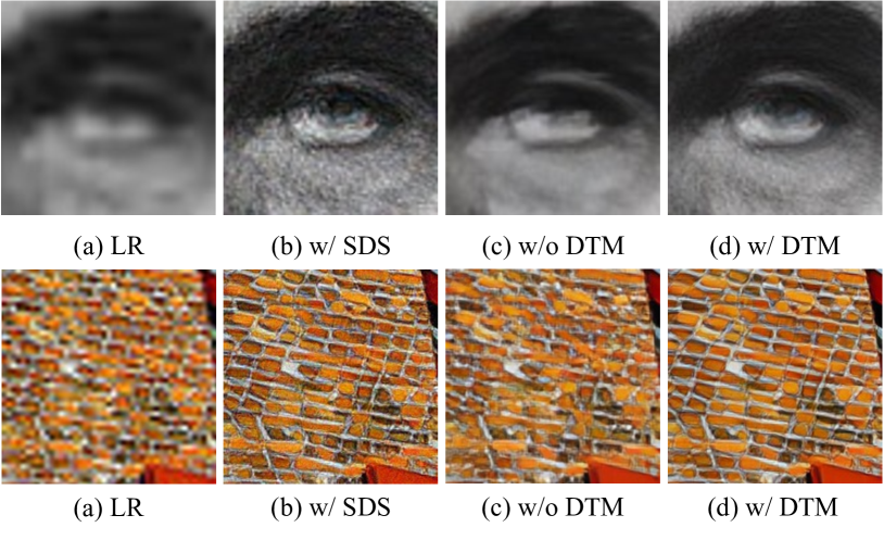
Figure 5: A visual comparison between the impact of DTM and SDS. It can be observed that DTM restores more details and produces fewer artifacts compared to the other two methods.

5 Conclusion

In this paper, we propose Consistency Trajectory Matching for Super-Resolution (CTMSR), an efficient method that enables generating high-realism SR results with only one inference step without the need for distillation. We first introduce the Consistency Training for SR to directly learn the deterministic mapping between the LR images perturbed with noise to HR images, thereby establishing a PF-ODE trajectory. To better align the distribution of SR results with the distribution of natural images, we propose Distribution Trajectory Matching (DTM) that matches their respective trajectories from LR distribution based on the learned PF-ODE, resulting in significant enhancements in the realism of SR results. Extensive experimental results demonstrate that our method achieves comparable or even better performance compared to existing diffusion-based methods while maintaining the fastest inference speed.

Supplementary Material

In the supplementary materials, we introduce more details of our implementation, more experimental results and more visual comparisons.

A. Implementation Details

A.1. Noise and Residual Schedules

Following [12], we design the schedule for $\sigma(t)$ as follows:

$$\sigma(t)=\sigma_{\text{max}}\cdot\left(\frac{t}{T}\right)^{\rho_{n}},$$ (22)

where $\sigma_{\text{max}}$ denotes the highest noise level and $\rho_{n}$ controls the speed of noise growth; a larger $\rho_{n}$ leads to faster growth in the earlier stages and slower growth in the later stages, and vice versa. Similarly, we also design a schedule for $\alpha(t)$:

$$\alpha(t)=\left(\frac{t}{T}\right)^{\rho_{r}},$$ (23)

where $\rho_{r}$ serves a role identical to that of $\rho_{n}$. In practice, we adopt the linear schedule by setting $\rho_{n}=1$ and $\rho_{r}=1$.

A.2. Step Schedule

We design a step schedule for Consistency Training of our SR model that adjusts the number of steps with the growth of training iterations. In contrast to  [28, 30], we utilize a linearly decreasing curriculum for the total steps $T$, rather than an increasing one. Specifically, the curriculum is formulated as follows:

$$T(k)=\text{max}(s_{0}-\lfloor\frac{k}{K^{\prime}}\rfloor,s_{1}),\quad K^{\prime}=\left\lfloor\frac{K}{s_{0}-s_{1}+1}\right\rfloor,$$ (24)

where $k$ denotes the training iteration, $s_{0}$ denotes the initial steps, $s_{1}$ denotes the final steps and $K$ denotes the total iterations. We empirically discover that the decreasing step schedule could produce better results and achieve faster convergence with $s_{0}=4,s_{1}=3$.

A.3. Training Details of Distribution Trajectory Matching

To stabilize the training of DTM, we propose to periodically update $\bm{f}_{\bm{\theta}^{\prime}}$. Specifically, we update $\bm{f}_{\bm{\theta}^{\prime}}$ with the parameters of $\bm{f}_{\bm{\theta}}$ every 1k iterations during the training stage of DTM. Algorithm 3 shows the details of the overall training process of CTMSR and Algorithm  3 shows the implementation of Distribution Trajectory Matching loss.

Algorithm 2 Overall training procedure of CTMSR.

0:  training CTMSR $\bm{f}_{\bm{\theta}}(\cdot)$

0:  Paired training dataset $(X,Y)$

1:  Stage 1: Consistency Training for One-Step SR

2:  $k\leftarrow 0$

3:  while not converged do

4:   $\bm{\theta}^{-}\leftarrow\text{stopgrad}(\bm{\theta})$

5:   sample $\bm{x}_{0},\bm{y}_{0}\sim(X,Y)$

6:   sample $t\sim U(0,T(k)-1)$

7:   compute $\bm{x}_{t},\bm{x}_{t-1}$ using Eq. 1

8:   $\mathcal{L}_{\text{CT}}=d(\bm{f}_{\bm{\theta}}(\bm{x}_{t},\bm{y}_{0},t),\bm{f}_{\bm{\theta}^{-}}(\bm{x}_{t-1},\bm{y}_{0},t-1))$

9:   Take a gradient descent step on $\nabla_{\theta}\mathcal{L}_{\text{CT}}$

10:   $k\leftarrow k+1$

11:  end while

12:  Stage 2: Distribution Trajectory Matching

13:  $\bm{\theta}^{\prime}\leftarrow\text{stopgrad}(\bm{\theta})$

14:  while not converged do

15:   if $k\equiv 0\pmod{1000}$ then

16:    $\bm{f}_{\bm{\theta}^{\prime}}\leftarrow\bm{f}_{\bm{\theta}}$

17:   end if

18:   sample $\bm{x}_{0},\bm{y}_{0}\sim(X,Y)$

19:   sample $t^{\prime}\sim U(1,T(k))$

20:   compute $\bm{x}_{t^{\prime}}$ using Eq. 1

21:   $\hat{\bm{x}}_{0}=\bm{f}_{\bm{\theta}}(\bm{x}_{t^{\prime}},\bm{y}_{0},t^{\prime})$

22:   sample $t\sim U(T_{\text{min}},T_{\text{max}})$

23:   compute $\bm{x}_{t},\hat{\bm{x}}_{t}$ using Eq. 1

24:   $\textbf{grad}=\omega(t)(\bm{f}_{\bm{\theta}^{\prime}}(\hat{\bm{x}}_{t},\bm{y}_{0},t)-\bm{f}_{\bm{\theta}^{\prime}}(\bm{x}_{t},\bm{y}_{0},t)$

25:   $\mathcal{L}_{\mathrm{DTM}}=0.5*\text{LPIPS}(\bm{\hat{x}}_{0},\text{stopgrad}(\bm{\hat{x}}_{0}-\textbf{grad}))$

26:   $\mathcal{L}_{\text{total}}=\lambda_{\text{CT}}\mathcal{L}_{\text{CT}}\ +\ \lambda_{\text{DTM}}\mathcal{L}_{\text{DTM}}$

27:   Take a gradient descent step on $\nabla_{\theta}\mathcal{L}_{\text{total}}$

28:   $k\leftarrow k+1$

29:  end while

30:  return  Converged CTMSR $f_{\theta}(\cdot)$.

Algorithm 3 Distribution Trajectory Matching Loss.

0:  pre-trained CTMSR $\bm{f}_{\bm{\theta^{\prime}}}(\cdot)$, HR image $\bm{x}_{0}$, LR image $\bm{y}_{0}$, timestep intervals ($T_{\text{min}},T_{\text{max}}$), SR output $\bm{\hat{x}}_{0}$

1:  sample $t\sim U(T_{\text{min}},T_{\text{max}})$

2:  compute $\bm{x}_{t},\hat{\bm{x}}_{t},\omega(t)$

3:  $\textbf{grad}=\omega(t)(\bm{f}_{\bm{\theta}^{\prime}}(\hat{\bm{x}}_{t},\bm{y}_{0},t)-\bm{f}_{\bm{\theta}^{\prime}}(\bm{x}_{t},\bm{y}_{0},t)$)

4:  $\mathcal{L}_{\mathrm{DTM}}=0.5*\text{LPIPS}(\bm{\hat{x}}_{0},\text{stopgrad}(\bm{\hat{x}}_{0}-\textbf{grad}))$

5:  return  $\mathcal{L}_{\mathrm{DTM}}$

A.4. Overall Training Process

The training process of our CTMSR can be broadly divided into two stages as mentioned in the main paper. In the first stage, we train our model exclusively with $\mathcal{L}_{\text{CT}}$ until convergence. Then we utilize a weighted combination of $\mathcal{L}_{\text{CT}}$ and $\mathcal{L}_{\text{DTM}}$ to further optimize our model. The total loss is formulated as:

$$\mathcal{L}_{\text{total}}=\lambda_{\text{CT}}\mathcal{L}_{\text{CT}}\ +\ \lambda_{\text{DTM}}\mathcal{L}_{\text{DTM}},$$ (25)

where we assign $\lambda_{\text{CT}}=1$ and $\lambda_{\text{DTM}}=1.6$. The overall training process is summarized in Algorithm 2.

B. More Experimental Results

B.1. Ablation Study

To comprehensively demonstrate the effectiveness of the proposed DTM, we present additional experimental results of the ablation study on ImageNet-Test, RealSet65 and RealSR datasets. The results demonstrate the effectiveness of DTM across synthetic and real-world datasets. The detailed results are shown in Table 5, 6, 7.

B.2. Compared with SinSR

The test results on RealSet65 and RealSR (shown in Table 2) demonstrate that our method outperforms SinSR [36] across all metrics except for CLIPIQA. Upon detailed observation, we discover that the CLIPIQA tends to favor images with noise or artifacts and sometimes fails to distinguish between fine image details and noise or artifacts. Therefore, CLIPIQA occasionally produces higher scores for images of lower quality due to the presence of noise or artifacts. The visual examples are shown in Figure 6.

B.3. Compared with Stable Diffusion-Based Methods

Though Stable Diffusion-based methods achieve impressive results, they rely on the powerful generative capabilities of Stable Diffusion (SD). This results in these methods being constrained by fixed backbones (Stable Diffusion), which limits their scalability to smaller models and consequently restricts their applicability in practical scenarios. In addition, these methods require extremely large models and incur significant inference costs, placing them in a different track from our approach. To compare with SD-based methods, we apply our approach to the latent space provided by VQ-VAE to further enhance the performance of our model. As shown in Table 8, our refined method attains performance on par with SD-based methods with much fewer model parameters and inference time. To be more specific, (1) OSEDiff demands 1.7 times the inference time and 8 times the number of model parameters; (2) AddSR demands 3.7 times the inference time and 10 times the number of model parameters.

B.3. Visual Comparison

We provide more visual examples of CTMSR compared with recent state-of-the-art methods on ImageNet-Test and real-world datasets. The visual examples are shown in Figure 7,  8,  9,  10  11,  12,  13.

Methods	PSNR$\uparrow$	LPIPS$\downarrow$	CLIPIQA$\uparrow$	MUSIQ$\uparrow$
CTMSR (w/o DTM)	24.71	0.2004	0.6092	56.650
CTMSR (w/ SDS)	23.17	0.2545	0.6292	58.188
CTMSR (w/ DTM)	24.73	0.1969	0.6913	60.142

Table 5: Experimental results of ablation study on ImageNet-Test.

Methods	CLIPIQA$\uparrow$	MUSIQ$\uparrow$	MANIQA$\uparrow$	NIQE$\downarrow$
CTMSR (w/o DTM)	0.6009	64.274	0.3658	4.37
CTMSR (w/ SDS)	0.6446	62.217	0.3606	4.77
CTMSR (w/ DTM)	0.6893	67.173	0.4360	4.51

Table 6: Experimental results of ablation study on RealSet65.

Methods	CLIPIQA$\uparrow$	MUSIQ$\uparrow$	MANIQA$\uparrow$	NIQE$\downarrow$
CTMSR (w/o DTM)	0.5542	62.351	0.3512	4.33
CTMSR (w/ SDS)	0.6101	60.919	0.3479	5.11
CTMSR (w/ DTM)	0.6449	64.796	0.4157	4.65

Table 7: Experimental results of ablation study on RealSR.

Methods	Runtime (s)	Params (M)	CLIPIQA$\uparrow$	MUSIQ$\uparrow$	MANIQA$\uparrow$
OSEDiff	0.3100	1775	0.6693	69.10	0.4717
AddSR	0.6857	2280	0.5410	63.01	0.4113
CTMSR	0.1847	225	0.7420	64.81	0.4810

Table 8: Quantitative comparisons with SD-based methods on RealSR. The runtime is tested on $128\times 128$ input images.

Figure 6: An illustration of CLIPIQA’s tendency to favor images with noise or artifacts and its inability to effectively distinguish between fine image details and noise or artifacts. Here are two visual examples of CTMSR and SinSR.

Figure 7: Visual comparison of different methods on ImageNet-Test. Please zoom in for more details.

Figure 8: Visual comparison of different methods on ImageNet-Test. Please zoom in for more details.

Figure 9: Visual comparison of different methods on ImageNet-Test. Please zoom in for more details.

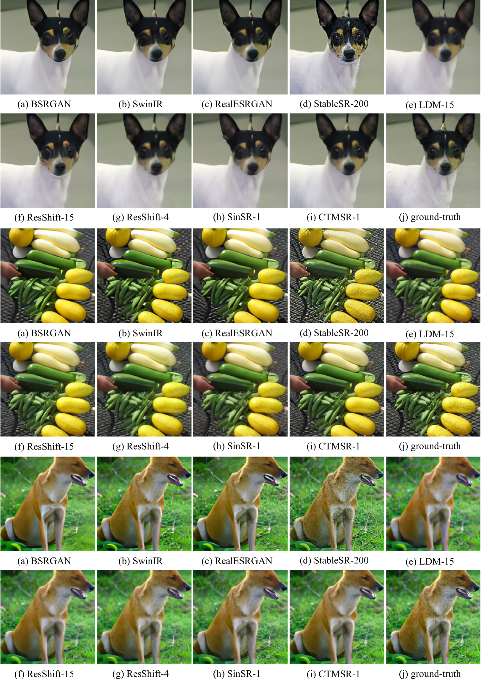
Figure 10: Visual comparison of different methods on ImageNet-Test. Please zoom in for more details.

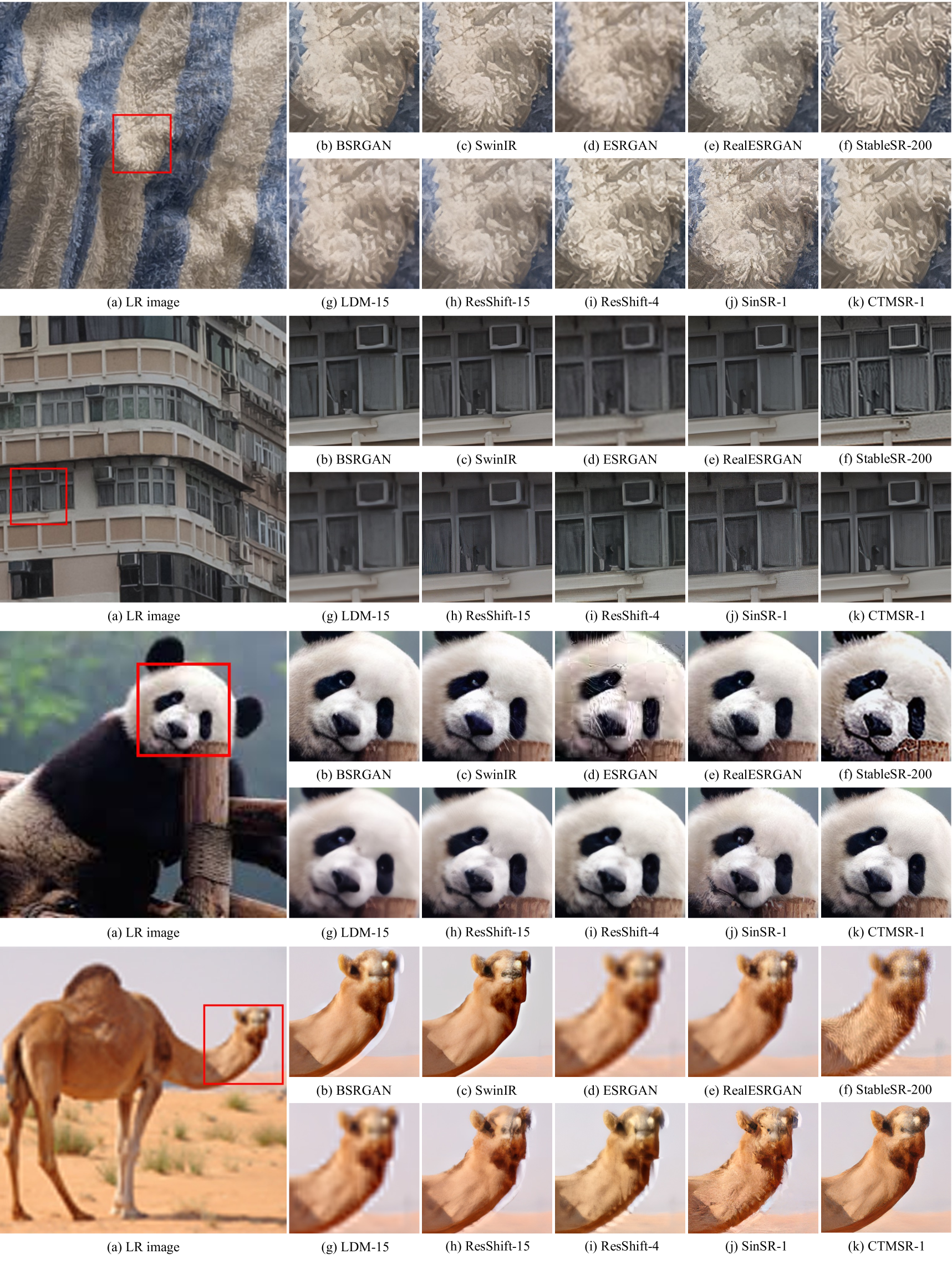
Figure 11: Visual comparison of different methods on real-world datasets. Please zoom in for more details.

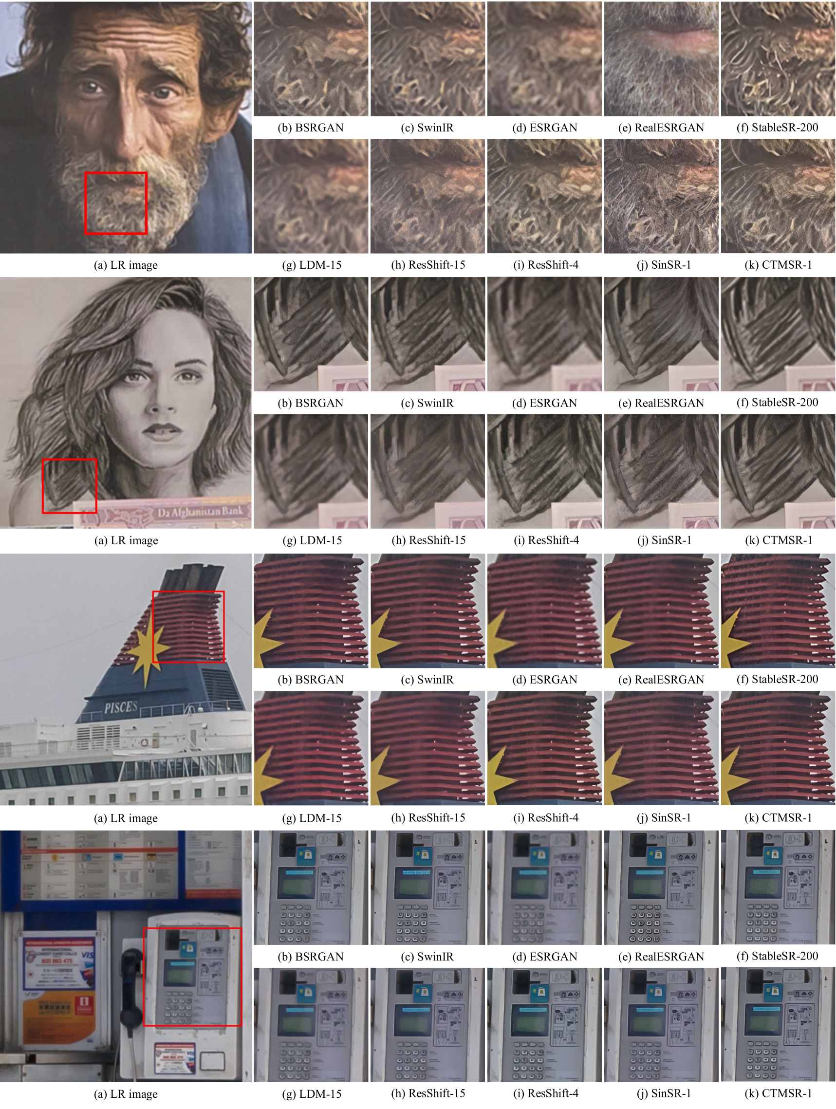
Figure 12: Visual comparison of different methods on real-world datasets. Please zoom in for more details.

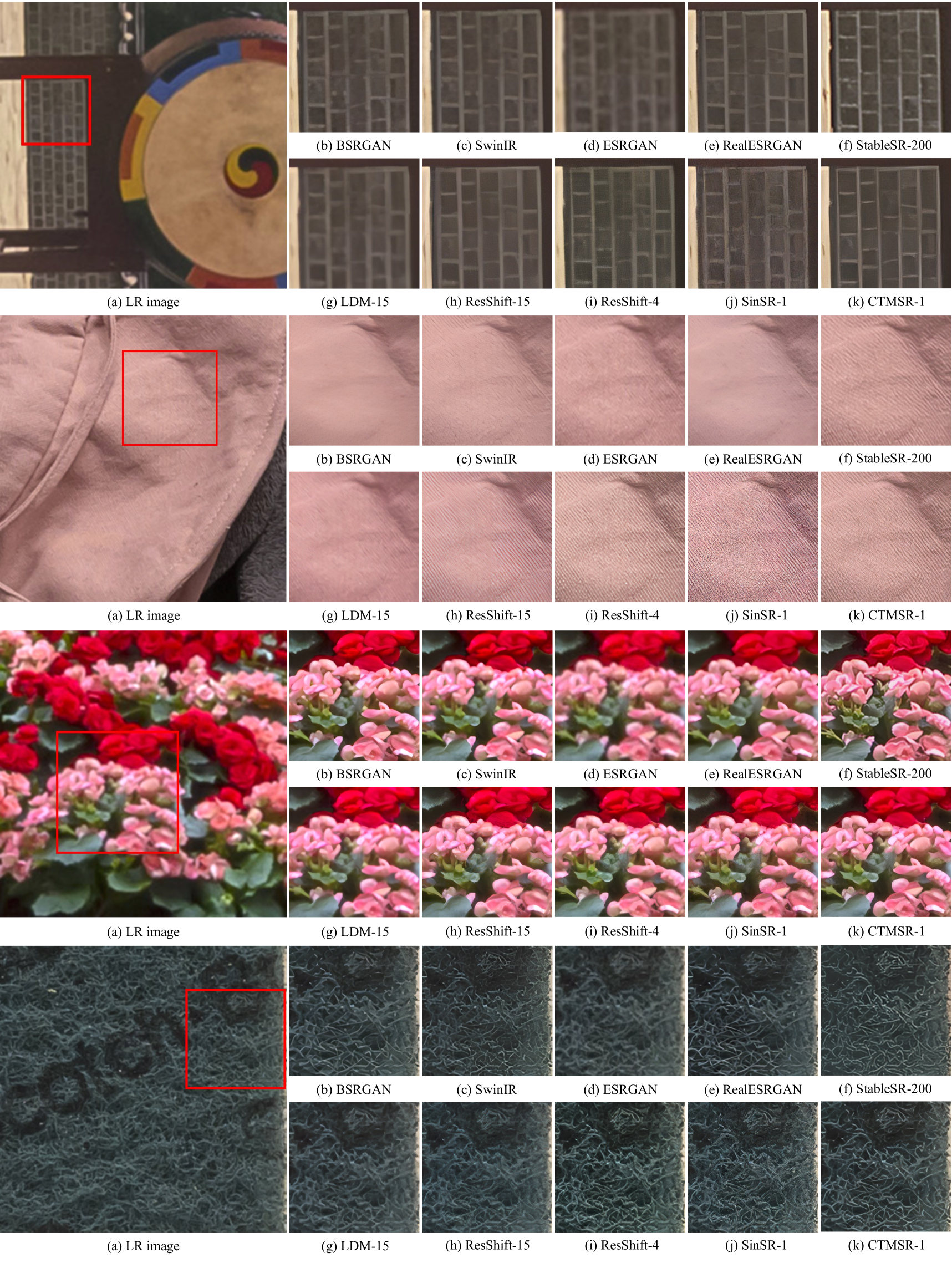
Figure 13: Visual comparison of different methods on real-world datasets. Please zoom in for more details.

References

- Cai et al. [2019] Jianrui Cai, Hui Zeng, Hongwei Yong, Zisheng Cao, and Lei Zhang. Toward real-world single image super-resolution: A new benchmark and a new model. In Proceedings of the IEEE/CVF international conference on computer vision, pages 3086–3095, 2019.
- Charbonnier et al. [1997] Pierre Charbonnier, Laure Blanc-Féraud, Gilles Aubert, and Michel Barlaud. Deterministic edge-preserving regularization in computed imaging. IEEE Transactions on image processing, 6(2):298–311, 1997.
- Chen et al. [2023] Xiangyu Chen, Xintao Wang, Jiantao Zhou, Yu Qiao, and Chao Dong. Activating more pixels in image super-resolution transformer. In Proceedings of the IEEE/CVF conference on computer vision and pattern recognition, pages 22367–22377, 2023.
- Choi et al. [2021] Jooyoung Choi, Sungwon Kim, Yonghyun Jeong, Youngjune Gwon, and Sungroh Yoon. Ilvr: Conditioning method for denoising diffusion probabilistic models. arXiv preprint arXiv:2108.02938, 2021.
- Deng et al. [2009] Jia Deng, Wei Dong, Richard Socher, Li-Jia Li, Kai Li, and Li Fei-Fei. Imagenet: A large-scale hierarchical image database. In 2009 IEEE conference on computer vision and pattern recognition, pages 248–255. Ieee, 2009.
- Dong et al. [2015] Chao Dong, Chen Change Loy, Kaiming He, and Xiaoou Tang. Image super-resolution using deep convolutional networks. IEEE transactions on pattern analysis and machine intelligence, 38(2):295–307, 2015.
- Dong et al. [2012] Weisheng Dong, Lei Zhang, Guangming Shi, and Xin Li. Nonlocally centralized sparse representation for image restoration. IEEE transactions on Image Processing, 22(4):1620–1630, 2012.
- Esser et al. [2021] Patrick Esser, Robin Rombach, and Bjorn Ommer. Taming transformers for high-resolution image synthesis. In Proceedings of the IEEE/CVF conference on computer vision and pattern recognition, pages 12873–12883, 2021.
- Gu et al. [2015] Shuhang Gu, Wangmeng Zuo, Qi Xie, Deyu Meng, Xiangchu Feng, and Lei Zhang. Convolutional sparse coding for image super-resolution. In Proceedings of the IEEE International Conference on Computer Vision, pages 1823–1831, 2015.
- Hertz et al. [2023] Amir Hertz, Kfir Aberman, and Daniel Cohen-Or. Delta denoising score. In Proceedings of the IEEE/CVF International Conference on Computer Vision, pages 2328–2337, 2023.
- Ho et al. [2020] Jonathan Ho, Ajay Jain, and Pieter Abbeel. Denoising diffusion probabilistic models. Advances in neural information processing systems, 33:6840–6851, 2020.
- Karras et al. [2022] Tero Karras, Miika Aittala, Timo Aila, and Samuli Laine. Elucidating the design space of diffusion-based generative models. Advances in neural information processing systems, 35:26565–26577, 2022.
- Kawar et al. [2022] Bahjat Kawar, Michael Elad, Stefano Ermon, and Jiaming Song. Denoising diffusion restoration models. Advances in Neural Information Processing Systems, 35:23593–23606, 2022.
- Ke et al. [2021] Junjie Ke, Qifei Wang, Yilin Wang, Peyman Milanfar, and Feng Yang. Musiq: Multi-scale image quality transformer. In Proceedings of the IEEE/CVF international conference on computer vision, pages 5148–5157, 2021.
- Ledig et al. [2017] Christian Ledig, Lucas Theis, Ferenc Huszár, Jose Caballero, Andrew Cunningham, Alejandro Acosta, Andrew Aitken, Alykhan Tejani, Johannes Totz, Zehan Wang, et al. Photo-realistic single image super-resolution using a generative adversarial network. In Proceedings of the IEEE conference on computer vision and pattern recognition, pages 4681–4690, 2017.
- Li et al. [2022] Haoying Li, Yifan Yang, Meng Chang, Shiqi Chen, Huajun Feng, Zhihai Xu, Qi Li, and Yueting Chen. Srdiff: Single image super-resolution with diffusion probabilistic models. Neurocomputing, 479:47–59, 2022.
- Li et al. [2023] Yawei Li, Yuchen Fan, Xiaoyu Xiang, Denis Demandolx, Rakesh Ranjan, Radu Timofte, and Luc Van Gool. Efficient and explicit modelling of image hierarchies for image restoration. In Proceedings of the IEEE/CVF Conference on Computer Vision and Pattern Recognition, pages 18278–18289, 2023.
- Liang et al. [2021] Jingyun Liang, Jiezhang Cao, Guolei Sun, Kai Zhang, Luc Van Gool, and Radu Timofte. Swinir: Image restoration using swin transformer. In Proceedings of the IEEE/CVF international conference on computer vision, pages 1833–1844, 2021.
- Liu et al. [2022] Xingchao Liu, Chengyue Gong, and Qiang Liu. Flow straight and fast: Learning to generate and transfer data with rectified flow. arXiv preprint arXiv:2209.03003, 2022.
- Lu et al. [2022] Cheng Lu, Yuhao Zhou, Fan Bao, Jianfei Chen, Chongxuan Li, and Jun Zhu. Dpm-solver: A fast ode solver for diffusion probabilistic model sampling in around 10 steps. Advances in Neural Information Processing Systems, 35:5775–5787, 2022.
- Luo et al. [2023] Ziwei Luo, Fredrik K Gustafsson, Zheng Zhao, Jens Sjölund, and Thomas B Schön. Image restoration with mean-reverting stochastic differential equations. arXiv preprint arXiv:2301.11699, 2023.
- Nichol and Dhariwal [2021] Alexander Quinn Nichol and Prafulla Dhariwal. Improved denoising diffusion probabilistic models. In International conference on machine learning, pages 8162–8171. PMLR, 2021.
- Poole et al. [2022] Ben Poole, Ajay Jain, Jonathan T Barron, and Ben Mildenhall. Dreamfusion: Text-to-3d using 2d diffusion. arXiv preprint arXiv:2209.14988, 2022.
- Rombach et al. [2022] Robin Rombach, Andreas Blattmann, Dominik Lorenz, Patrick Esser, and Björn Ommer. High-resolution image synthesis with latent diffusion models. In Proceedings of the IEEE/CVF conference on computer vision and pattern recognition, pages 10684–10695, 2022.
- Saharia et al. [2022] Chitwan Saharia, Jonathan Ho, William Chan, Tim Salimans, David J Fleet, and Mohammad Norouzi. Image super-resolution via iterative refinement. IEEE transactions on pattern analysis and machine intelligence, 45(4):4713–4726, 2022.
- Salimans and Ho [2022] Tim Salimans and Jonathan Ho. Progressive distillation for fast sampling of diffusion models. arXiv preprint arXiv:2202.00512, 2022.
- Song et al. [2020a] Jiaming Song, Chenlin Meng, and Stefano Ermon. Denoising diffusion implicit models. arXiv preprint arXiv:2010.02502, 2020a.
- Song and Dhariwal [2023] Yang Song and Prafulla Dhariwal. Improved techniques for training consistency models. arXiv preprint arXiv:2310.14189, 2023.
- Song et al. [2020b] Yang Song, Jascha Sohl-Dickstein, Diederik P Kingma, Abhishek Kumar, Stefano Ermon, and Ben Poole. Score-based generative modeling through stochastic differential equations. arXiv preprint arXiv:2011.13456, 2020b.
- Song et al. [2023] Yang Song, Prafulla Dhariwal, Mark Chen, and Ilya Sutskever. Consistency models. arXiv preprint arXiv:2303.01469, 2023.
- Tian et al. [2024] Yuchuan Tian, Hanting Chen, Chao Xu, and Yunhe Wang. Image processing gnn: Breaking rigidity in super-resolution. In Proceedings of the IEEE/CVF Conference on Computer Vision and Pattern Recognition, pages 24108–24117, 2024.
- Wang et al. [2023] Jianyi Wang, Kelvin CK Chan, and Chen Change Loy. Exploring clip for assessing the look and feel of images. In Proceedings of the AAAI Conference on Artificial Intelligence, pages 2555–2563, 2023.
- Wang et al. [2024a] Jianyi Wang, Zongsheng Yue, Shangchen Zhou, Kelvin CK Chan, and Chen Change Loy. Exploiting diffusion prior for real-world image super-resolution. International Journal of Computer Vision, pages 1–21, 2024a.
- Wang et al. [2018] Xintao Wang, Ke Yu, Shixiang Wu, Jinjin Gu, Yihao Liu, Chao Dong, Yu Qiao, and Chen Change Loy. Esrgan: Enhanced super-resolution generative adversarial networks. In Proceedings of the European conference on computer vision (ECCV) workshops, pages 0–0, 2018.
- Wang et al. [2021] Xintao Wang, Liangbin Xie, Chao Dong, and Ying Shan. Real-esrgan: Training real-world blind super-resolution with pure synthetic data. In Proceedings of the IEEE/CVF international conference on computer vision, pages 1905–1914, 2021.
- Wang et al. [2024b] Yufei Wang, Wenhan Yang, Xinyuan Chen, Yaohui Wang, Lanqing Guo, Lap-Pui Chau, Ziwei Liu, Yu Qiao, Alex C Kot, and Bihan Wen. Sinsr: diffusion-based image super-resolution in a single step. In Proceedings of the IEEE/CVF Conference on Computer Vision and Pattern Recognition, pages 25796–25805, 2024b.
- Wang et al. [2004] Zhou Wang, Alan C Bovik, Hamid R Sheikh, and Eero P Simoncelli. Image quality assessment: from error visibility to structural similarity. IEEE transactions on image processing, 13(4):600–612, 2004.
- Wang et al. [2024c] Zhengyi Wang, Cheng Lu, Yikai Wang, Fan Bao, Chongxuan Li, Hang Su, and Jun Zhu. Prolificdreamer: High-fidelity and diverse text-to-3d generation with variational score distillation. Advances in Neural Information Processing Systems, 36, 2024c.
- Wu et al. [2025] Rongyuan Wu, Lingchen Sun, Zhiyuan Ma, and Lei Zhang. One-step effective diffusion network for real-world image super-resolution. Advances in Neural Information Processing Systems, 37:92529–92553, 2025.
- Xie et al. [2024] Rui Xie, Chen Zhao, Kai Zhang, Zhenyu Zhang, Jun Zhou, Jian Yang, and Ying Tai. Addsr: Accelerating diffusion-based blind super-resolution with adversarial diffusion distillation. arXiv preprint arXiv:2404.01717, 2024.
- Yang et al. [2022] Sidi Yang, Tianhe Wu, Shuwei Shi, Shanshan Lao, Yuan Gong, Mingdeng Cao, Jiahao Wang, and Yujiu Yang. Maniqa: Multi-dimension attention network for no-reference image quality assessment. In Proceedings of the IEEE/CVF Conference on Computer Vision and Pattern Recognition, pages 1191–1200, 2022.
- Yin et al. [2024] Tianwei Yin, Michaël Gharbi, Richard Zhang, Eli Shechtman, Fredo Durand, William T Freeman, and Taesung Park. One-step diffusion with distribution matching distillation. In Proceedings of the IEEE/CVF Conference on Computer Vision and Pattern Recognition, pages 6613–6623, 2024.
- Yue et al. [2024] Zongsheng Yue, Jianyi Wang, and Chen Change Loy. Resshift: Efficient diffusion model for image super-resolution by residual shifting. Advances in Neural Information Processing Systems, 36, 2024.
- Zeyde et al. [2012] Roman Zeyde, Michael Elad, and Matan Protter. On single image scale-up using sparse-representations. In Curves and Surfaces: 7th International Conference, Avignon, France, June 24-30, 2010, Revised Selected Papers 7, pages 711–730. Springer, 2012.
- Zhang et al. [2021] Kai Zhang, Jingyun Liang, Luc Van Gool, and Radu Timofte. Designing a practical degradation model for deep blind image super-resolution. In Proceedings of the IEEE/CVF International Conference on Computer Vision, pages 4791–4800, 2021.
- Zhang et al. [2015] Lin Zhang, Lei Zhang, and Alan C Bovik. A feature-enriched completely blind image quality evaluator. IEEE Transactions on Image Processing, 24(8):2579–2591, 2015.
- Zhang et al. [2024] Leheng Zhang, Yawei Li, Xingyu Zhou, Xiaorui Zhao, and Shuhang Gu. Transcending the limit of local window: Advanced super-resolution transformer with adaptive token dictionary. In Proceedings of the IEEE/CVF Conference on Computer Vision and Pattern Recognition (CVPR), pages 2856–2865, 2024.
- Zhang et al. [2018] Richard Zhang, Phillip Isola, Alexei A Efros, Eli Shechtman, and Oliver Wang. The unreasonable effectiveness of deep features as a perceptual metric. In Proceedings of the IEEE conference on computer vision and pattern recognition, pages 586–595, 2018.
- Zhao et al. [2024] Wenliang Zhao, Lujia Bai, Yongming Rao, Jie Zhou, and Jiwen Lu. Unipc: A unified predictor-corrector framework for fast sampling of diffusion models. Advances in Neural Information Processing Systems, 36, 2024.
- Zhou et al. [2020] Yuanbo Zhou, Wei Deng, Tong Tong, and Qinquan Gao. Guided frequency separation network for real-world super-resolution. In Proceedings of the IEEE/CVF Conference on Computer Vision and Pattern Recognition Workshops, pages 428–429, 2020.