Fixed points and critical temperature near quantum critical points in $d$-wave cuprate superconductors

Abstract

We study the critical behavior driven by potential quantum critical points (QCPs) termed as $\tau_{0,x,y,z}$-Type QCPs beneath the superconducting dome of the $d$-wave cuprate superconductors. To comprehensively capture the distinct degrees of freedom in the vicinity of these QCPs, we construct a phenomenological effective theory based on the Landau-Ginzburg-Wilson framework and then employ the renormalization group approach to derive the coupled flow equations of all interaction parameters, incorporating all relevant one-loop corrections. Decoding these flow equations yields a series of unique properties arising from strong quantum fluctuations around QCPs. On one hand, the interaction parameters flow toward several fixed points (FPs) at certain critical energy scales. We identify two different types of FPs designated at the clean limit. FP-I is characterized by the divergence of the quadratic parameter and exhibits robustness against variations in interaction parameters. In contrast, FP-II is dominated by the cubic and quartic interaction parameters, and it is sensitive to initial conditions, leading to five subclasses: FP-IIA, FP-IIB, FP-IIC, FP-IID, and FP-IIE. Besides, we find that disorder scattering can influence fermion velocities and critical energy scales, and even destabilize certain FPs around the $\tau_{x,z}$-QCPs, driving the system toward a preempted disorder-induced FP. On the other hand, we find that quantum fluctuations play a critical role in shaping the critical temperature ($T_{c}$) as the system approaches these QCPs. Near the $\tau_{x}$-QCP, $T_{c}$ is considerably suppressed for both FP-I and FP-II. In contrast, near the $\tau_{0}$-QCP, $T_{c}$ undergoes a substantial decrease for FP-I but only a slight decrease for FP-II. Conversely, $T_{c}$ exhibits an increasing trend near the $\tau_{y}$-QCP, with a pronounced peak at $v_{\Delta 0}/v_{F0}\sim 0.25$. However, numerical analysis suggests that the $\tau_{z}$-QCP is unlikely to be physically realizable. Additionally, we realize that $T_{c}$ can also be modified by the emergence of disorder-induced FPs in the vicinity of the $\tau_{x}$-QCP. These findings would provide valuable insights into the critical low-energy properties of $d$-wave cuprate superconductors and related materials.

I Introduction

The study of $d$-wave cuprate superconductors has garnered significant theoretical and experimental interest over the past three decades Lee2006RMP ; Vojta2000PRL ; Vojta2000PRB ; Vojta2000IJMPB ; Sachdev2000Science ; Sachdev2003RMP ; Sachdev2008PRB ; Sachdev2011PT ; Wang2011PRB ; Fradkin2012NPhys ; Kivelson2014PNAS ; Fradkin2015RMP ; Dagotto1994RMP ; Dagotto2005Science ; Kivelson1995Nature ; Kivelson1998Nature ; Kivelson2003RMP_DFS ; Sigrist1991RMP ; Sigrist1995RMP ; Tinkham1996Book ; Anderson1997Book ; Phillips2020NPhys ; Kim-Kivelson2008PRB ; She2010PRB ; She2015PRB ; Xu2008PRB ; Larkin2005Book ; Takagi1992PRL ; Norman2011Science ; Shekhter2013Nature ; Bozovic2016Nature ; Phiillips2022Science ; Ramakrishnan2025 . These materials are renowned for their unconventional pairing mechanisms, the anomalous behavior of their normal, and the coexistence of multiple phases below the critical temperature Lee2006RMP ; Sachdev2003RMP ; Kivelson2014PNAS ; Fradkin2015RMP ; Kivelson1998Nature ; Norman2011Science ; Shekhter2013Nature ; Phiillips2022Science ; Ramakrishnan2025 . Notably, they exhibit a distinct $d_{x^{2}-y^{2}}$ superconducting gap Lee2006RMP ; Ding1996Nature ; Loeser1996Science ; Valla1999Science ; Orenstein2000Science ; Yoshida2003PRL ; Dagotto1994RMP , which vanishes at four points ($\pm\pi/2,\pm\pi/2$) in the first Brillouin zone known as the nodal points Lee2006RMP ; Fradkin2015RMP ; Dagotto1994RMP . At these nodal points, gapless quasiparticles (QPs) are excited even at the lowest-energy limit under the superconducting dome Orenstein2000Science ; Sachdev2000Science ; Sachdev2003RMP ; Lee2006RMP ; Sachdev2011PT . Besides, the coexistence of different phases is usually accompanied by some quantum phase transition (QPT) Vojta2003RPP ; Sachdev2011Book ; Coleman2005Nature , during which certain critical bosonic modes can emerge.

The QPs are typically considered nearly non-interacting, but they can couple to critical bosonic modes near a QPT due to strong quantum fluctuations Vojta2000PRB ; Vojta2000PRL ; Vojta2000IJMPB ; Paaske2001PRL ; Kim-Kivelson2008PRB ; Sachdev2008PRB ; Xu2008PRB ; Sachdev2009PRB ; Liu2012PRB ; Liu2013NJP ; She2015PRB . These quantum critical degrees of freedom are assumed to play a pivotal role in the anomalous behavior observed in $d$-wave superconductors  Orenstein2000Science ; Coleman2005Nature ; Lee2006RMP ; Fradkin2012NPhys ; Kivelson2014PNAS ; Fradkin2015RMP ; Sachdev2011Book ; Vojta2003RPP ; Moon2010PRB ; Moon2012PRB ; Moon2016PRB ; Moon2016SRep ; Wang-EM2014PRB ; Yoshida2003PRL ; Paaske2001PRL ; Sachdev2009PRB ; Liu2012PRB ; Liu2013NJP . Several theoretical frameworks have been proposed to study the interplay between quantum criticality and the QPs in these compounds Lee1993PRL ; Vojta2000PRL ; Vojta2000PRB ; Coleman2005Nature ; Dagotto2005Science ; Sachdev2000Science ; Sachdev2011PT ; Castellani1997ZPB ; She2011PRL . In particular, Vojta et al. Vojta2000PRL ; Vojta2000PRB ; Vojta2000IJMPB suggest the existence of a quantum critical point (QCP) within the superconducting dome Sachdev2011Book ; Vojta2003RPP . This QCP marks a transition from the $d_{x^{2}-y^{2}}$ superconducting state to a new state denoted by $d_{x^{2}-y^{2}}+X$ as illustrated in Fig. 1, where the $X$ state is associated with certain a symmetry breaking. The group-theory analysis Vojta2000PRL ; Vojta2000PRB ; Vojta2000IJMPB identifies several potential candidates, which can be further categorized into four distinct types, namely, $\tau_{0}$-Type, $\tau_{x}$-Type, $\tau_{y}$-Type, and $\tau_{z}$-Type QCPs Vojta2000PRL ; Vojta2000PRB ; Wang2013PRB .

In recent years, significant efforts have been devoted to studying these QCPs in $d$-wave superconductors Sachdev2008PRB ; Kim-Kivelson2008PRB ; Xu2008PRB ; Vojta2009AP ; Sachdev2002PRB ; Kivelson2009PRB ; Sachdev2010PRB ; Fradkin2010ARCMP ; Kivelson1998Nature ; Kivelson2001PRB ; Vojta2000PRB ; Vojta2000PRL ; Sachdev2009PRB ; Kim2010PRB ; Wang2011PRB . Among these, the $\tau_{x}$-Type QCP attracted considerable attention, which is related to a nematic QPT with breaking $C_{4}$ symmetry down to $C_{2}$ symmetry Keimer2008Science ; Kim2010Nature ; Sachdev2011Book ; Kivelson1998Nature ; Metzner2000PRL ; Kivelson2001PRB . In particular, Huh and Sachdev Sachdev2008PRB carefully examine the tendencies of fermion velocities ($v_{F,\Delta}$) nearby the $\tau_{x}$-Type QCP. Then, the fates of $v_{F,\Delta}$ as approaching the $\tau_{y}$-Type and $\tau_{z}$-Type QCPs have also been investigated Wang2013PRB ; Wang2015PLA ; Wang2013NJP and identified distinct kinds of fixed points for fermion velocities in the lowest-energy regime. These unusual behavior of fermion velocities are expected to play a crucial role in shaping the low-energy physical quantities Lee1993PRL ; Durst2000PRB ; Mesot1999PRL ; Vojta2009AP ; Kim-Kivelson2008PRB ; Xu2008PRB ; Wang2011PRB ; Wang2013PRB ; Wang2015PLA ; Wang2013NJP ; She2015PRB ; RZW2022NPB ; Durst2000PRB .

While important progress Sachdev2008PRB ; Wang2013PRB ; Kim-Kivelson2008PRB ; Xu2008PRB ; Wang2011PRB ; Wang2015PLA ; Wang2013NJP ; Liu2012PRB ; She2015PRB ; RZW2022NPB has been made in understanding the critical behavior near these QPTs, several intriguing issues remain to be addressed to fully characterize the quantum criticality in the vicinity of these QCPs. On one hand, to simplify the analysis, the underlying quantum fluctuations of SC order are usually neglected in previous studies. However, as the system approaches the QCP, quantum criticality can coax this very ingredient to mutually interact with other degrees of freedom. As studied in Refs. Kleinert2003NPB ; Wang2014PRD ; Wang2017PRB , the amplitude and phase fluctuations of a complex scalar field can ferociously compete with other kinds of fields, leading to non-trivial critical effects. In principle, the SC order parameter in $d$-superconductor can be described by a complex scalar field, which yields both the amplitude and phase fluctuations nearby the QCP. These fluctuations are expected to couple with those of the $X$-state order parameter, and their mutual interactions can influence all other interaction parameters. As a consequence, this coupling can be expected to significantly modify the low-energy behavior of the QCPs. On the other hand, most previous studies have focused on the $\tau_{x}$-type QCP, leaving the critical properties of other candidate QCPs ($\tau_{y}$, $\tau_{z}$, and $\tau_{0}$ types) insufficiently explored. Besides, it is particularly important to determine whether these candidate QCPs can emerge under physically realistic conditions, despite being theoretically possible from the perspective of group theory. Furthermore, as the system approaches physically realizable QCPs, it is crucial to investigate how the critical temperature is affected by the interplay between quantum fluctuations of the $X$-order parameter and those of the superconducting order parameter.

These interesting issues motivate us to systematically investigate the critical consequences and distinctions among various types of QCPs on the physics of related quantum critical regions. This requires us to consider the combination of strong quantum fluctuations of all order parameters and their interplay with other degrees of freedom. In order to take into account these ingredients unbiasedly, we employ the momentum-shell renormalization group (RG) approach Shankar1994RMP ; Wilson1975RMP ; Polchinski1992 , which equally treats all relevant critical degrees of freedom near the putative QPT from a $d$-wave superconducting state to a $d_{x^{2}-y^{2}}+X$ state, as illustrated in Fig. 1. By incorporating all one-loop corrections, we derive a set of coupled RG equations for all the interaction parameters. These equations provide detailed insights into the quantum critical behavior near the candidate QCPs.

We commence with performing a numerical analysis of these flow equations. The results indicate that the overall tendencies of the interaction parameters are dictated by several fixed points (FPs) that are designated in Sec. IV at certain critical energy scale $l=l_{c}$ depending on the initial conditions. These fixed points are closely linked to the low-energy critical behavior of the system. In the clean limit, the system evolves toward two distinct types of fixed points: FP-I and FP-II. FP-I is characterized by the divergence of the quadratic parameter, which remains largely independent of other interaction parameters. In contrast, FP-II is dominated by the cubic and quartic interaction parameters, and it is sensitive to alterations in interaction parameters, yielding five subclasses, i.e., FP-IIA, FP-IIB, FP-IIC, FP-IID, and FP-IIE, due to the strong competition among order parameters. In addition, we examine the stabilities of these FPs in the presence of three types of disorder scattering: random mass, random gauge potential, and random chemical potential. Numerical analysis demonstrates that both random mass and random gauge potential provide negligible impacts on FPs. However, the random chemical potential can significantly influence both the fermion velocities and the critical energy scales. This may lead to the emergence of a preempted disorder-induced fixed point, as illustrated in Fig. 9.

To proceed, we systematically investigate the behavior of critical temperature ($T_{c}$) as accessing FPs for all QCPs in Fig. 1. A detailed analysis demonstrates that $T_{c}$ around $\tau_{x}$-QCP is significantly suppressed for both FP-I and FP-II. In contrast, nearby $\tau_{0}$-QCP, it undergoes a substantial decrease for FP-I but only a slight decrease for FP-II. Interestingly, $T_{c}$ exhibits an increasing trend near the $\tau_{y}$-QCP, with a pronounced peak at $v_{\Delta 0}/v_{F0}\sim 0.25$. This indicates that the initial anisotropy of the fermion velocities ($v_{\Delta 0}/v_{F0}$) can also quantitatively influence $T_{c}$. Additionally, we notice that $T_{c}$ is insensitive to both random mass and random gauge potential but can be considerably altered by the random chemical potential in the vicinity of $\tau_{x}$-QCP. Regarding the $\tau_{z}$-QCP, we find that the enhancement of $T_{c}$ lies well beyond the range of critical temperatures $T_{c}$ typically observed in $d$-wave superconductors Lee2006RMP ; Fradkin2015RMP ; Keimer2008Science ; Orenstein2000Science ; Bozovic2016Nature ; Phiillips2022Science ; Ramakrishnan2025 . This suggests that such a QCP is unlikely to be physically realizable.

The remainder of this paper is organized as follows. In Sec. II, we establish a low-energy effective field theory to describe the physical properties surrounding the QCP in Fig. 1. By adopting the standard procedure of RG framework, we within Sec. III derive the coupled RG equations of all interacting parameters. Sec. IV presents a systematic analysis of the low-energy behavior of these interaction parameters and identifies distinct fixed points as the system approaches four candidate QCPs. In Sec. V, we carefully examine the effects of quantum fluctuations and competing orders on the critical temperature of $d$-wave superconductor near the QCPs. Finally, we provide a concise summary of our results in Sec. VI.

II Effective theory

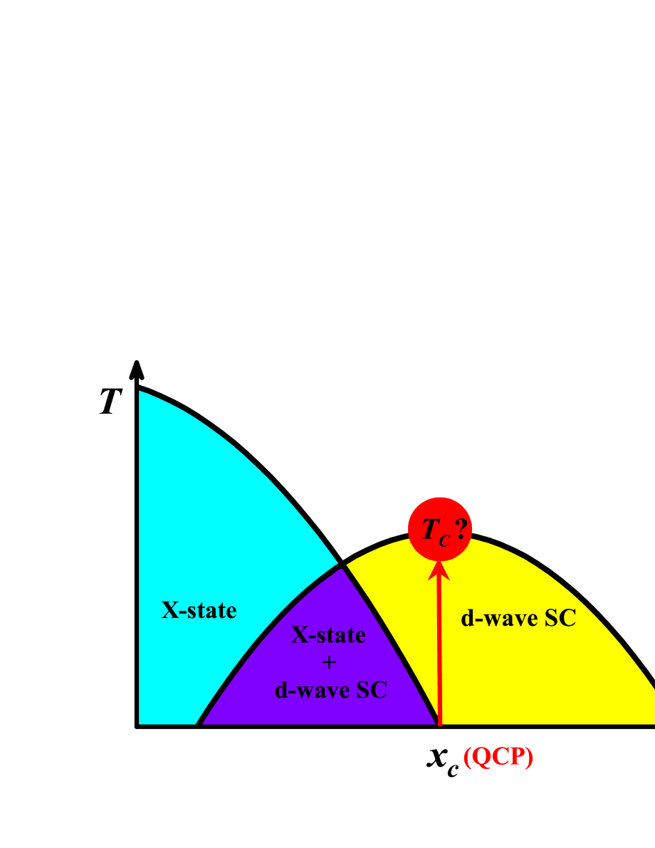
Figure 1: (Color online) Schematic illustration for an underlying quantum phase transition (QPT) between the $d$-wave superconducting (SC) state and an $X$ state with certain symmetry breaking beneath the SC dome via tuning the non-thermal doping variable Vojta2000PRL ; Vojta2000PRB ; Vojta2000IJMPB ; Sachdev2011PT . Here, $T_{c}$ represents the critical temperature that is dependent upon the doping, while the point $x_{c}$ denotes the quantum critical point (QCP) nearby the optimal doping, which separates the ordered $X$ state plus $d-$wave SC and the pure $d$-wave SC. Within the quantum critical region above the QCP, the critical behavior would be expected owing to the strong quantum fluctuations induced by the QPT, which will be presented in Sec. V.

We within this work put our focus on the critical behavior around the quantum critical point (QCP) in the superconducting dome of $d$-wave superconductor. As schematically illustrated in Fig. 1, there exist distinct kinds of degrees of freedom that interact with each other in the vicinity of the QCP, including the gapless fermionic quasiparticles (QPs) and the fluctuations of order parameters as well as the disorder scatterings. To be specific, the fermionic sector takes the form of Sachdev2008PRB ,

$$S_{\Psi}\!\! = \!\!\int\!\!\frac{d^{2}\mathbf{k}}{(2\pi)^{2}}\frac{d\omega}{2\pi}\Psi^{{\dagger}}_{1a}(-i\omega\!+\!v_{F}k_{x}\tau_{z}\!+\!v_{\Delta}k_{y}\tau_{x})\Psi_{1a}$$ (1)

$$\!\!\!\!\!\!+\!\!\int\!\!\frac{d^{2}\mathbf{k}}{(2\pi)^{2}}\frac{d\omega}{2\pi}\Psi^{{\dagger}}_{2a}(-i\omega\!+\!v_{F}k_{y}\tau_{z}\!\!+\!v_{\Delta}k_{x}\tau_{x})\Psi_{2a},$$

with $\tau_{x,y,z}$ being Pauli matrices. Here, $\Psi^{\dagger}_{1a}$ denotes two gapless QPs excited from the nodes at $(\frac{\pi}{2}$,$\frac{\pi}{2})$ and $(-\frac{\pi}{2}$,$-\frac{\pi}{2})$, while $\Psi^{\dagger}_{2a}$ describes the QPs from the other two nodes Vojta2000PRL ; Vojta2000PRB ; Vojta2000IJMPB ; Sachdev2008PRB . Besides, $k_{x,y}$ represent two mutually perpendicular momenta, and $v_{F,\Delta}$ specify the Fermi velocity and the gap velocity, respectively. To proceed, we are going to present the remaining parts in the Eq. (38) one by one in the following subsections.

II.1 Fluctuations of order parameters

As depicted in Fig. 1, the superconducting dome is separated into two distinct regions owing to the QPT . For the right side, it corresponds to the $d$-wave superconducting (SC) state. In comparison, the $X$-state order parameter emerges on the left side accompanied by certain symmetry breaking. In the vicinity of the QCP, the fluctuations of order parameters can bring important contributions to the critical behavior.

At first, let us consider the fluctuation of $X$ state denoted by $\phi$. In principle, there exist four distinct kinds of $X$ states due to different symmetry breakings Vojta2000PRL ; Vojta2000PRB ; Vojta2000IJMPB , which are helpful to cluster the four sorts of potential QCPs at $x_{c}$, namely $\tau_{x,y,z}$-QCP and $\tau_{0}$-QCP. These fluctuations can interact with the fermionic QPs nearby QCPs Vojta2000PRL ; Vojta2000PRB ; Vojta2000IJMPB ; RZW2022NPB ,

$$S_{\Psi\phi}=\begin{cases}\int d^{2}\mathbf{x}d\tau[\lambda_{0}\phi(\Psi^{{\dagger}}_{1}\mathcal{M}_{1}\Psi_{1}+\Psi^{{\dagger}}_{2}\mathcal{M}_{2}\Psi_{2})],\\ \int d^{2}\mathbf{x}d\tau[\lambda_{0}(\phi_{0A}\Psi^{{\dagger}}_{1}\mathcal{M}_{1}\Psi_{1}+\phi_{0B}\Psi^{{\dagger}}_{2}\mathcal{M}_{2}\Psi_{2})],\end{cases}$$ (2)

with $\lambda_{0}$ specifying the coupling strength. Hereby, $\phi$ together with $\phi_{0A,0B}$ denote the $X$-state fluctuations and the matrices $\mathcal{M}_{1,2}$ characterize unique features of related QCPs, namely $\mathcal{M}_{1,2}=\tau_{x},\tau_{y},\tau_{z}$ and $\mathcal{M}_{1,2}=\tau_{0}$ corresponding to $\tau_{x,y,z}$-QCP and $\tau_{0}$-QCP that owns two components $\phi_{0A}$ and $\phi_{0B}$, respectively Vojta2000PRL ; Vojta2000PRB ; Vojta2000IJMPB .

As to the free part of $X$ state, it generally can be written as follows,

$$S_{\phi} = \frac{1}{2}\int\frac{d^{3}q}{(2\pi)^{3}}(-2r+q^{2})\phi^{2},$$ (3)

where $\phi^{2}$ are replaced by $(\phi_{0A}^{2}+\phi_{0B}^{2})$ for the $\tau_{0}$-QCP and the parameter $r$ measures the distance away from the QCP. It is worth highlighting that one-loop corrections due to the interplay $S_{\Psi\phi}$ can qualitatively modifies such a free part. As shown in Refs. Sachdev2008PRB ; Wang2013PRB ; Wang2013NJP , one-loop polarization of the order parameter of $X$ state can be expressed as

$$\Pi^{x}(\mathbf{q}) = \frac{1}{16v_{F}v_{\Delta}}\frac{\varepsilon^{2}+v^{2}_{F}q_{x}^{2}}{\sqrt{\varepsilon^{2}+v^{2}_{F}q_{x}^{2}+v^{2}_{\Delta}q_{y}^{2}}}+(q_{x}\leftrightarrow q_{y}),$$ (4)

$$\Pi^{y}(\mathbf{q}) = \frac{1}{16v_{F}v_{\Delta}}\sqrt{\varepsilon^{2}+v^{2}_{F}q_{x}^{2}+v^{2}_{\Delta}q_{y}^{2}}+(q_{x}\leftrightarrow q_{y}),$$ (5)

$$\Pi^{z}(\mathbf{q}) = \frac{1}{16v_{F}v_{\Delta}}\frac{\varepsilon^{2}+v^{2}_{\Delta}q_{y}^{2}}{\sqrt{\varepsilon^{2}+v^{2}_{F}q_{x}^{2}+v^{2}_{\Delta}q_{y}^{2}}}+(q_{x}\leftrightarrow q_{y}),$$ (6)

and

$$\Pi^{0}_{A}(q_{x},q_{y}) = -\frac{1}{16v_{F}v_{\Delta}}\sqrt{\varepsilon^{2}+v^{2}_{F}q_{x}^{2}+v^{2}_{\Delta}q_{y}^{2}},$$ (7)

$$\Pi^{0}_{B}(q_{y},q_{x}) = -\frac{1}{16v_{F}v_{\Delta}}\sqrt{\varepsilon^{2}+v^{2}_{F}q_{y}^{2}+v^{2}_{\Delta}q_{x}^{2}}.$$ (8)

It can be found that $\Pi^{i}(q)$ with $i=0,x,y,z$ is proportional to $q$ and hence it dominates over the dynamic term with a quadratic $q$ in the low-energy region. In addition, the parameter $r$ is negligible as we primarily focus on the physics nearby the QCP shown in Fig. 1. Accordingly, the low-energy “free term” of $X$ state can be recast into

$$S_{\phi} = \frac{1}{2}\int\frac{d^{3}q}{(2\pi)^{3}}[\Pi^{i}(q)]\phi^{2},$$ (9)

which yields the renormalized propagator of $X$-state order parameter,

$$G_{\phi}(q)=\frac{1}{\Pi^{i}(q)}.$$ (10)

with $i=\tau_{x,y,z,0}$ for distinct kinds of QCPs.

Next, we move to consider the fluctuation of SC order parameter. Generally, the competition between SC and $X$-state order parameters takes the form of Wang2013NJP ; Wang2014PRD ; Kleinert2003NPB

$$\mathcal{L}_{\mathrm{compe}} = \mathcal{L}_{\psi}+\mathcal{L}_{\phi}+\mathcal{L}_{\psi\phi},$$ (11)

with

$$\mathcal{L}_{\psi} = \partial_{\mu}\psi^{\dagger}\partial_{\mu}\psi-\alpha|\psi|^{2}+\frac{\beta}{2}|\psi|^{4},$$ (12)

$$\mathcal{L}_{\phi} = \frac{1}{2}(\partial_{\mu}\phi)^{2}-2r\phi^{2}+\frac{u}{2}\phi^{4},$$ (13)

$$\mathcal{L}_{\psi\phi} = \lambda|\psi|^{2}\phi^{2},$$ (14)

where $\psi$ describes the SC order parameter and $\alpha,\beta,\gamma,u$ are the related parameters. As approaching the QCP shown in Fig. 1, it is of particular importance to point out that $\psi$ acquires a finite vacuum expectation value due to vacuum degeneracy Kleinert2003NPB ,

$$\langle\psi\rangle\equiv V_{0}=\sqrt{\frac{\alpha}{\beta}}.$$ (15)

In order to capture the SC fluctuation around such an expectation value, we introduce two gapless field $h$ and $\eta$ to specify the amplitude fluctuation and the phase fluctuation, respectively. Accordingly, the $\psi$ can be reexpressed as Kleinert2003NPB

$$\psi=V_{0}+\frac{1}{\sqrt{2}}(h+i\eta).$$ (16)

where $\langle h\rangle=\langle\eta\rangle=0$ and their free propagators can be obtained as

$$G_{h}(k) = \frac{1}{k^{2}+2\alpha_{h}},$$ (17)

$$G_{\eta}(k) = \frac{1}{k^{2}}.$$ (18)

Then, after inserting Eq. (16) into Eqs. (11)-(14), as well as combining Eq. (1) and Eq. (2), and carrying out several calculations with discarding the unimportant constant terms, we are finally left with the following Wang2013NJP ; Wang2014PRD ; Kleinert2003NPB effective action,

$$S_{\mathrm{eff}} = S_{\Psi}+S_{\phi}+S_{h}+S_{\eta}+S_{\Psi\phi}+S_{\eta^{2}h}$$ (19)

$$+S_{\phi^{2}h}+S_{h^{2}\eta^{2}}+S_{h^{2}\phi^{2}}+S_{\eta^{2}\phi^{2}}.$$

Here, $S_{\Psi}$, $S_{\phi}$, and $S_{h,\eta}$ correspond to the contributions from fermionic QPs, $X$-state, and superconducting of fluctuations, respectively. Besides, the other terms collect the interactions among these distinct kinds of degrees of freedom. Specifically, they are written as

$$S_{\phi} = \int\frac{d^{2}\mathbf{q}d\varepsilon}{(2\pi)^{3}}[2\alpha_{\phi}+\Pi^{i}(\mathbf{q},\varepsilon)]\phi^{2}$$ (20)

$$+\frac{\beta_{\phi}}{2}\int\prod_{m=1}^{4}\frac{d^{2}\mathbf{q}_{m}d\varepsilon_{m}}{(2\pi)^{3}}\mathcal{X}(m)\phi^{4},$$

$$S_{h} = \int\frac{d^{2}\mathbf{k}d\omega}{(2\pi)^{3}}(2\alpha_{h}+\mathbf{k}^{2}+\omega^{2})h^{2}$$ (21)

$$+\gamma_{h}\int\prod_{m=1}^{3}\frac{d^{2}\mathbf{k}_{m}d\omega_{m}}{(2\pi)^{3}}\mathcal{X}(m)h^{3}$$

$$+\frac{\beta_{h}}{2}\int\prod_{m=1}^{4}\frac{d^{2}\mathbf{k}_{m}d\omega_{m}}{(2\pi)^{3}}\mathcal{X}(m)h^{4},$$

$$S_{\eta} = \int\frac{d^{2}\mathbf{k}d\omega}{(2\pi)^{3}}(\mathbf{k}^{2}+\omega^{2})\eta^{2}$$ (22)

$$+\frac{\beta_{\eta}}{2}\int\prod_{m=1}^{4}\frac{d^{2}\mathbf{k}_{m}d\omega_{m}}{(2\pi)^{3}}\mathcal{X}(m)\eta^{4},$$

$$S_{\eta^{2}h} = \gamma_{\eta h}\int\prod_{i=1,2}\frac{d^{2}\mathbf{k}_{i}d\omega_{i}}{(2\pi)^{3}}\frac{d^{2}\mathbf{k}^{\prime}d\omega^{\prime}}{(2\pi)^{3}}$$ (23)

$$\times\eta(\mathbf{k}_{i},\omega_{i})h(\mathbf{k}^{\prime},\omega^{\prime})\mathcal{Y}^{(\mathbf{k},\mathbf{k}^{\prime})}_{(\omega,\omega^{\prime})},$$

$$S_{\phi^{2}h} = \gamma_{\phi h}\int\prod_{i=1,2}\frac{d^{2}\mathbf{q}_{i}d\varepsilon_{i}}{(2\pi)^{3}}\frac{d^{2}\mathbf{k}d\omega}{(2\pi)^{3}}$$ (24)

$$\times\phi(\mathbf{q}_{i},\varepsilon_{i})h(\mathbf{k},\omega)\mathcal{Y}^{(\mathbf{q},\mathbf{k})}_{(\varepsilon,\omega)},$$

$$S_{h^{2}\eta^{2}} = \lambda_{\eta h}\int\prod_{i=1,2}\frac{d^{2}\mathbf{k}_{i}d\omega_{i}d^{2}\mathbf{k}_{i}^{\prime}d\omega_{i}^{\prime}}{(2\pi)^{6}}$$ (25)

$$\times\eta(\mathbf{k}_{i},\omega_{i})h(\mathbf{k}_{i}^{\prime},\omega_{i}^{\prime})\mathcal{Z}^{(\mathbf{k},\mathbf{k}^{\prime})}_{(\omega,\omega^{\prime})},$$

$$S_{h^{2}\phi^{2}} = \lambda_{h\phi}\int\prod_{i=1,2}\frac{d^{2}\mathbf{k}_{i}d\omega_{i}d^{2}\mathbf{q}_{i}d\varepsilon_{i}}{(2\pi)^{6}}$$ (26)

$$\times h(\mathbf{k}_{i},\omega_{i})\phi(\mathbf{q}_{i},\varepsilon_{i})\mathcal{Z}^{(\mathbf{k},\mathbf{q})}_{(\omega,\varepsilon)},$$

$$S_{\eta^{2}\phi^{2}} = \lambda_{\eta\phi}\int\prod_{i=1,2}\frac{d^{2}\mathbf{k}_{i}d\omega_{i}d^{2}\mathbf{q}_{i}d\varepsilon_{i}}{(2\pi)^{6}}$$ (27)

$$\times\eta(\mathbf{k}_{i},\omega_{i})\phi(\mathbf{q}_{i},\varepsilon_{i})\mathcal{Z}^{(\mathbf{k},\mathbf{q})}_{(\omega,\varepsilon)},$$

where the related coefficients are designated as

$$\alpha_{h} = \alpha,\quad\alpha_{\phi}=\lambda\alpha/\beta+r,$$ (28)

$$\beta_{h} = \beta_{\eta}=\beta/4,\quad\beta_{\phi}=u,$$ (29)

$$\gamma_{h} = \gamma_{\eta h}=\sqrt{2\alpha\beta}/2,\quad\gamma_{\phi h}=\lambda\sqrt{2\alpha/\beta},$$ (30)

$$\lambda_{\eta h} = \beta/4,\quad\lambda_{h\phi}=\lambda_{\eta\phi}=\lambda/2,$$ (31)

$$\mathcal{X}(m) \equiv \delta^{2}(\Sigma\mathbf{k}_{m})\delta(\Sigma\omega_{m}),$$ (32)

$$\mathcal{Y}^{(\mathbf{a},\mathbf{b})}_{(p,q)} \equiv \delta^{2}(\mathbf{a}_{1}\!+\!\mathbf{a}_{2}\!+\!\mathbf{b})\delta(p_{1}\!+\!p_{2}\!+\!q),$$ (33)

$$\mathcal{Z}^{(\mathbf{a},\mathbf{b})}_{(p,q)} \equiv \delta^{2}(\mathbf{a}_{1}\!+\!\mathbf{a}_{2}\!+\!\mathbf{b}_{1}\!+\!\mathbf{b}_{2})\delta(p_{1}\!+\!p_{2}\!+\!q_{1}\!+\!q_{2}).$$ (34)

II.2 Disorder scatterings and total effective action

In real systems, disorder scatterings may also be of particular importance Lee1985RMP ; Mirlin2008RMP ; Nersesyan1995NPB ; Fiete2016PRB ; Efremov11 . Without loss of generality, we consider the disorder $A(\mathbf{x})$ is a quneched, Gaussian white noise potential, which is defined by the following correction functions Nersesyan1995NPB ,

$$\langle A(\mathbf{x})\rangle = 0,$$ (35)

$$\langle A(\mathbf{x_{1}})A(\mathbf{x_{2}})\rangle = g\delta^{2}(\mathbf{x_{1}}-\mathbf{x_{2}}),$$ (36)

where the parameter $g$ represents the concentration of impurity. It therefore yields the interplay between fermionic QPs and disorder as Nersesyan1995NPB ; Stauber2005PRB

$$S_{\mathrm{dis}} = v_{\Gamma}\int d^{2}\mathbf{x}\Psi^{\dagger}(\mathbf{x})\Gamma\Psi(\mathbf{x})A(\mathbf{x}),$$ (37)

where $v_{\Gamma}$ measures the strength of fermion-disorder coupling and the matrix $\Gamma$ characterizes the feature of disorder. Specifically, $\Gamma=\tau_{0}$, $\Gamma=\tau_{y}$, and $\Gamma=(\tau_{x},\tau_{z})$ corresponds to a random chemical potential, a random mass, and a random gauge potential, respectively Nersesyan1995NPB ; Stauber2005PRB ; Wang2011PRB .

In order to capture all these ingredients, we add the disorder scatterings (37) into $S_{\mathrm{eff}}$ (19) and arrive at the total phenomenological effective theory around the QCP in Fig. 1,

$$S^{\star}_{\mathrm{eff}}=S_{\mathrm{eff}}+S_{\mathrm{dis}}.$$ (38)

We are going to start from this effective action and carry out the RG analysis armed with the one-loop corrections as well as unreveal the potential critical behavior induced by the QCP below the SC dome in the forthcoming sections.

III RG analysis

On the basis of the effective action (38), we employ the Wilsonian momentum-shell RG method Wilson1975RMP ; Polchinski1992 ; Shankar1994RMP to establish the energy-dependent flows of all interaction parameters as approaching the QCP. These evolutions carry the low-energy information and are closely associated with the critical behavior.

Following the RG formalism Wilson1975RMP ; Polchinski1992 ; Shankar1994RMP , we need to integrate out the high-energy modes (fast modes) of fields in the effective theory (38) to obtain the one-loop corrections arising from all the interactions. Such fast modes are confined to a momentum shell $b\Lambda<k<\Lambda$ where $\Lambda$ represents an ultraviolet cutoff and $b$ is designated as $b=e^{-l}$ with $l$ being a running scale that goes towards infinity at the lowest energy Shankar1994RMP ; Kim2008PRB ; Huh2008PRB ; She2010PRB ; She2015PRB ; Wang2011PRB ; Wang2013PRB ; Wang2014PRD ; Wang2015PRB ; Wang2017PRB ; Wang2017QBCP ; Vafek2012PRB ; Vafek2014PRB ; Wang2022SST . For convenience, we rescale the momenta and energy by $\Lambda$, i.e., $k\rightarrow k/\Lambda$ and $\omega\rightarrow\omega=\omega/\Lambda$. Then, after lengthy but straightforward algebraic calculations, we obtain the one-loop corrections, which are presented in Appendix A.

In order to perform the RG analysis, we subsequently consider the RG rescaling transformations of momenta, energy, and fields that connect successive steps of RG procedure Wilson1975RMP ; Polchinski1992 ; Shankar1994RMP . For the fermionic and the $X$-state parts, we assume that the $-i\omega$ term in $S_{\Psi}$ (1) and the Yukawa coupling $\lambda_{0}$ in $S_{\Psi\phi}$ (2) remain invariant under the RG transformations Shankar1994RMP ; Huh2008PRB ; Sachdev2011Book . In addition, the disorder distribution (36) is also invariant Wang2011PRB ; Nersesyan1995NPB ; Stauber2005PRB . These together yield the following RG transformations,

$$k \rightarrow k^{\prime}e^{-l},$$ (39)

$$\omega \rightarrow \omega^{\prime}e^{-l},$$ (40)

$$\Psi_{1,2}(k,\omega) \rightarrow \Psi^{\prime}_{1,2}(k^{\prime},\omega^{\prime})e^{\frac{1}{2}\int^{l}_{0}(4-\zeta_{f})dl},$$ (41)

$$\phi(k,\omega) \rightarrow \phi^{\prime}(k^{\prime},\omega^{\prime})e^{\frac{1}{2}\int^{l}_{0}(4-\zeta_{b})dl},$$ (42)

$$A(k) \rightarrow A^{\prime}(k^{\prime})e^{l}.$$ (43)

Hereby, $\zeta_{f}$ and $\zeta_{b}$ serve as the anomalous dimensions that are determined by one-loop corrections presented in Appendix A and are expressed as,

$$\zeta_{f} = (C_{g}-\lambda_{0}^{2}\mathcal{A}^{i}_{1}),$$ (44)

in tandem with

$$\zeta_{b}= 1+2\lambda_{0}^{2}(\mathcal{A}^{i}_{1}+\mathcal{R}^{i}),\!\! \Gamma=\tau_{0}$$ (45)

$$\zeta_{b}= 1+2\lambda_{0}^{2}(\mathcal{A}^{i}_{1}+\mathcal{R}^{i})-4C_{g},\!\! \Gamma=\tau_{y}$$ (46)

$$\zeta_{b}= 1+2\lambda_{0}^{2}(\mathcal{A}^{i}_{1}+\mathcal{R}^{i})-2C_{g},\!\! \Gamma=\tau_{x}$$ (47)

$$\zeta_{b}= 1+2\lambda_{0}^{2}(\mathcal{A}^{i}_{1}+\mathcal{R}^{i})-2C_{g},\!\! \Gamma=\tau_{z}$$ (48)

where $\Gamma=\tau_{0,y,x,z}$ corresponds to different kinds of disorders and $C_{g}$ is defined as

$$C_{g} \equiv \frac{gv_{\Gamma}^{2}}{2\pi v_{F}v_{\Delta}}.$$ (49)

Hereby, the relevant coefficients $\mathcal{A}^{i}_{1}$ and $\mathcal{R}^{i}$ are designated in Appendix A, with the superscript $i=\tau_{x,y,z,0}$ denoting the type $\tau_{x,y,z,0}-$QCP discussed in Sec. II.1. Under these transformations, the field $h$ and $\eta$ that characterize the SC part should transform accordingly so that the free parts of actions $S_{h}$ and $S_{\eta}$ remain unchanged. As a consequence, $h$ and $\eta$ can be rescaled as Wang2014PRD ; Wang2022SST ; Wang2017PRB-FeSC ; Kleinert2003NPB

$$h(\mathbf{k},\omega) \rightarrow h^{\prime}(\mathbf{k^{\prime}},\omega^{\prime})e^{\frac{5}{2}l},$$ (50)

$$\eta(\mathbf{k},\omega) \rightarrow \eta^{\prime}(\mathbf{k^{\prime}},\omega^{\prime})e^{\frac{5}{2}l}.$$ (51)

To proceed, we are able to derive the coupled RG flows of all interaction parameters that dictate the critical behaviors around the QCP Shankar1994RMP ; Kim2008PRB ; Huh2008PRB ; She2010PRB ; She2015PRB ; Wang2011PRB by combining the above RG transformation scalings (39)-(51) with all one-loop corrections to interaction parameters detailed in Appendix A. For conciseness, we list the coupled RG equations for all interaction parameters near the type $i$-QCP, with the superscript $i=\tau_{x,y,z,0}$ respectively denoting the type $\tau_{x,y,z,0}-$QCP Shankar1994RMP ; Kim2008PRB ; Huh2008PRB ; She2010PRB ; She2015PRB ; Wang2011PRB ; Wang2013PRB ; Wang2014PRD ; Wang2015PRB ; Wang2017PRB ; Wang2017QBCP ; Vafek2012PRB ; Vafek2014PRB ; Wang2022SST ,

$$\frac{dv_{F}}{dl} = [\lambda_{0}^{2}(\mathcal{A}^{i}_{1}-\mathcal{A}^{i}_{2})-C_{g}]v_{F},$$ (52)

$$\frac{dv_{\Delta}}{dl} = [\lambda_{0}^{2}(\mathcal{A}^{i}_{1}-\mathcal{A}^{i}_{3})-C_{g}]v_{\Delta},$$ (53)

$$\frac{d\frac{v_{\Delta}}{v_{F}}}{dl} = \lambda_{0}^{2}(\mathcal{A}^{i}_{2}-\mathcal{A}^{i}_{3})(v_{\Delta}/v_{F}),$$ (54)

$$\frac{d\alpha_{h}}{dl} = 2\alpha_{h}+\frac{1}{4\pi^{2}}\left[-3\gamma_{h}^{2}-\gamma_{\eta h}^{2}-\frac{64}{\pi}\gamma_{\phi h}^{2}v_{F}^{2}v_{\Delta}^{2}\mathcal{F}^{i}_{2}(\theta,\varphi)+\frac{3}{4}\beta_{h}(1-2\alpha_{h})+\frac{1}{2}\lambda_{\eta h}+\frac{2v_{F}v_{\Delta}}{\pi}\lambda_{h\phi}\mathcal{F}^{i}_{1}(\theta,\varphi)\right],$$ (55)

$$\frac{d\gamma_{h}}{dl} = \frac{3}{2}\gamma_{h}+\frac{1}{4\pi^{2}}\left[8\gamma_{h}^{3}(1-6\alpha_{h})+\gamma_{h}\beta_{h}(1-4\alpha_{h})+\lambda_{\eta h}\gamma_{\eta h}+\frac{\lambda_{h\phi}\gamma_{\phi h}}{2\pi}(16v_{F}v_{\Delta})^{2}\mathcal{F}^{i}_{2}(\theta,\varphi)\right],$$ (56)

$$\frac{d\gamma_{\eta h}}{dl} = \frac{3}{2}\gamma_{\eta h}+\frac{1}{4\pi^{2}}\left[2\gamma_{\eta h}^{3}(1-2\alpha_{h})+\beta_{\eta}\gamma_{\eta h}+\frac{2\lambda_{\eta h}\gamma_{h}(1-4\alpha_{h})+\lambda_{\eta\phi}\gamma_{\phi h}}{2\pi}(16v_{F}v_{\Delta})^{2}\mathcal{F}^{i}_{2}(\theta,\varphi)\right],$$ (57)

$$\frac{d\gamma_{\phi h}}{dl} = \frac{(1-2\zeta_{b})}{2}\gamma_{\phi h}+\frac{1}{2\pi^{2}}\bigg{[}\frac{1}{4\pi}\gamma_{\phi h}^{3}(1-2\alpha_{h})(16v_{F}v_{\Delta})^{2}\mathcal{F}^{i}_{2}(\theta,\varphi)+\lambda_{h\phi}\gamma_{h}(1-4\alpha_{h})+\lambda_{\eta\phi}\gamma_{\eta h}$$ (58)

$$+\frac{\beta_{\phi}\gamma_{\phi h}}{8\pi}(16v_{F}v_{\Delta})^{2}\mathcal{F}^{i}_{2}(\theta,\varphi)\bigg{]},$$

$$\frac{d\beta_{h}}{dl} = \beta_{h}+\frac{1}{2\pi^{2}}\left[4\beta_{h}\gamma_{h}^{2}(1-6\alpha_{h})+\frac{\beta^{2}_{h}}{2}(1-4\alpha_{h})+2\lambda_{\eta h}^{2}+\frac{\lambda_{h\phi}^{2}}{2\pi}(16v_{F}v_{\Delta})^{2}\mathcal{F}^{i}_{2}(\theta,\varphi)\right],$$ (59)

$$\frac{d\beta_{\eta}}{dl} = \beta_{\eta}+\frac{1}{2\pi^{2}}\left[\beta_{\eta}\gamma_{\eta h}^{2}(1-2\alpha_{h})+\frac{\beta_{\eta}^{2}}{2}+2\lambda_{\eta h}^{2}(1-4\alpha_{h})+\frac{\lambda_{h\phi}^{2}}{2\pi}(16v_{F}v_{\Delta})^{2}\mathcal{F}^{i}_{2}(\theta,\varphi)\right],$$ (60)

$$\frac{d\beta_{\phi}}{dl} = -(1+2\zeta_{b})\beta_{\phi}+\frac{1}{2\pi^{2}}\bigg{[}\frac{1}{4\pi}\beta_{\phi}\gamma_{\phi h}^{2}(1-2\alpha_{h})(16v_{F}v_{\Delta})^{2}\mathcal{F}^{i}_{2}(\theta,\varphi)+2\lambda_{\phi h}^{2}(1-4\alpha_{h})$$ (61)

$$+2\lambda_{\eta\phi}^{2}+\frac{\beta^{2}_{\phi}}{8\pi}(16v_{F}v_{\Delta})^{2}\mathcal{F}^{i}_{2}(\theta,\varphi)\bigg{]},$$

$$\frac{d\lambda_{\eta h}}{dl} = \lambda_{\eta h}+\frac{1}{2\pi^{2}}\bigg{[}4\lambda_{\eta h}\gamma_{h}^{2}(1-6\alpha_{h})+\lambda_{\eta h}\gamma_{\eta h}^{2}(1-2\alpha_{h})+\frac{1}{2}\lambda_{\eta h}\beta_{h}(1-4\alpha_{h})+\frac{1}{2}\lambda_{\eta h}\beta_{\eta}$$ (62)

$$+\frac{1}{2}\lambda^{2}_{\eta h}(1-2\alpha_{h})+\frac{\lambda_{\eta\phi}\lambda_{h\phi}}{4\pi}(16v_{F}v_{\Delta})^{2}\mathcal{F}^{i}_{2}(\theta,\varphi)\bigg{]},$$

$$\frac{d\lambda_{h\phi}}{dl} = -\zeta_{b}\lambda_{h\phi}+\frac{1}{2\pi^{2}}\bigg{[}4\lambda_{h\phi}\gamma_{h}^{2}(1-6\alpha_{h})+\frac{1}{4\pi}\lambda_{h\phi}\gamma_{\phi h}^{2}(1-2\alpha_{h})(16v_{F}v_{\Delta})^{2}\mathcal{F}^{i}_{2}(\theta,\varphi)+\lambda_{\eta h}\lambda_{\eta\phi}+\frac{1}{2}\lambda_{h\phi}\beta_{h}(1-4\alpha_{h})$$ (63)

$$+\frac{\beta_{\phi}\lambda_{h\phi}}{8\pi}(16v_{F}v_{\Delta})^{2}\mathcal{F}^{i}_{2}(\theta,\varphi)+\frac{1}{8\pi}\lambda^{2}_{h\phi}(1-2\alpha_{h})(16v_{F}v_{\Delta})\mathcal{F}^{i}_{1}(\theta,\varphi)\bigg{]},$$

$$\frac{d\lambda_{\eta\phi}}{dl} = -\zeta_{b}\lambda_{\eta\phi}+\frac{1}{4\pi^{2}}\bigg{[}2\lambda_{\eta\phi}\gamma_{\eta h}^{2}(1-2\alpha_{h})+\frac{1}{2\pi}\lambda_{\eta\phi}\gamma_{\phi h}^{2}(1-2\alpha_{h})(16v_{F}v_{\Delta})^{2}\mathcal{F}^{i}_{2}(\theta,\varphi)-2\lambda_{\eta\phi}\lambda_{h\phi}(1-4\alpha_{h})+\beta_{\eta}\lambda_{\eta\phi}$$ (64)

$$+\frac{\beta_{\phi}\lambda_{\eta\phi}}{4\pi}(16v_{F}v_{\Delta})^{2}\mathcal{F}^{i}_{2}(\theta,\varphi)+\frac{1}{4\pi}\lambda^{2}_{\eta\phi}(16v_{F}v_{\Delta})\mathcal{F}^{i}_{1}(\theta,\varphi)\bigg{]},$$

in tandem with the flows of disorder couplings

$$\frac{dv_{\Gamma}}{dl}=0,\!\! \Gamma=\tau_{0}$$ (65)

$$\frac{dv_{\Gamma}}{dl}=(\lambda^{2}_{0}\mathcal{A}^{i}_{3}-\lambda^{2}_{0}\mathcal{A}^{i}_{2}-2C_{g})v_{\Gamma},\!\! \Gamma=\tau_{y}$$ (66)

$$\frac{dv_{\Gamma}}{dl}=(\lambda_{0}^{2}\mathcal{A}^{i}_{1}-\lambda^{2}_{0}\mathcal{A}^{i}_{3}-C_{g})v_{\Gamma},\!\! \Gamma=\tau_{x}$$ (67)

$$\frac{dv_{\Gamma}}{dl}=(\lambda_{0}^{2}\mathcal{A}^{i}_{1}-\lambda^{2}_{0}\mathcal{A}^{i}_{2}-C_{g})v_{\Gamma},\!\! \Gamma=\tau_{z}$$ (68)

where $\Gamma=\tau_{0,y,x,z}$ again corresponds to distinct kinds of disorders, and the related coefficients $\mathcal{A}^{i}_{1,2,3}$ and $\mathcal{F}^{i}_{1,2}$ with the superscript $i=\tau_{x,y,z,0}$ denoting the type $\tau_{x,y,z,0}-$QCP are provided in Appendix A. Hereby, it is necessary to stress that the Yukawa coupling $\lambda_{0}$ does not flow as it is chosen as the free fixed point Huh2008PRB . Besides, $\alpha_{\phi}$ in Eq. (20) is also considered to be a very small constant in that the focus is put on the quantum critical regime nearby the QCP Vojta2000PRL ; Vojta2000PRB ; Vojta2000IJMPB ; Sachdev2011PT ; Vojta2003RPP .

As approaching the QCP illustrated in Fig. 1, the interaction parameters couple intimately with each other through these RG evolutions (52)-(68). On one hand, the basic tendencies of the interaction parameters can be dictated by several fixed points as detailed in Sec. IV in the parameter space. On the other hand, the critical behavior near these fixed points may give rise to significant physical implications, such as the superfluid density and the critical temperature, which are influenced by the strong quantum fluctuations induced by the QCP. These will be addressed in the forthcoming Sec. V.

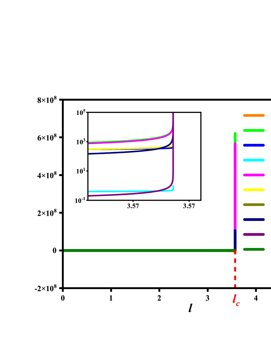
Figure 2: (Color online) Energy-dependent evolutions of interaction parameters for a representative initial condition around the $\tau_{x}$-QCP (the basic results are analogous for other kinds of QCPs). Hereby, the critical energy scale is denoted by $l_{c}$.

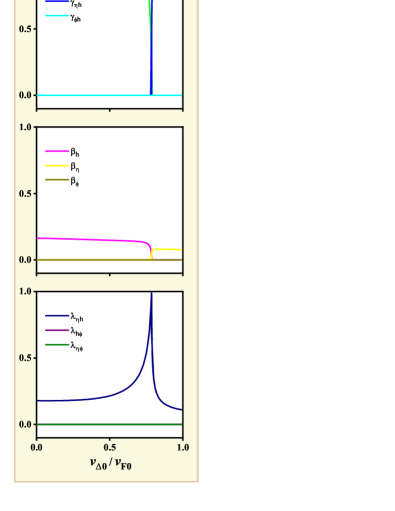
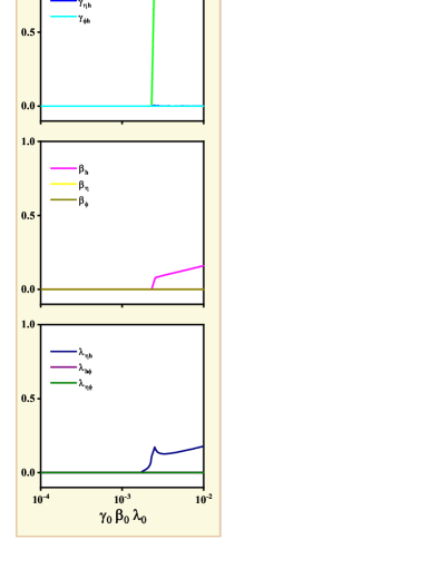
Figure 3: (Color online) Evolutions of the concrete values of FPs with variations of initial conditions: (a) the fermion velocities $v_{\Delta 0}/v_{F0}$ and (b) the interaction parameters $\gamma_{0}\beta_{0}\lambda_{0}$. The horizontal axis denotes the initial values of related parameters and the vertical axis represent the values of interaction parameters at the FP with $l=l_{c}$. With increasing $v_{\Delta 0}/v_{F0}$, the FP-IIA can be driven to the FP-IID, while decreasing $\gamma_{0}\beta_{0}\lambda_{0}$, it would be replaced by FP-I.

IV Fixed points driven by the quantum critical points

Starting from the coupled RG equations (52)-(68) that encapsulate the ordering competition among quantum fluctuations, we are now in a proper position to investigate the low-energy tendencies of all parameters around the distinct kinds of QCPs.

IV.1 Fixed points and classification

To investigate the energy-dependent tendencies of interaction parameters, we perform a numerical analysis of the coupled RG flow equations (52)-(68). For a representative initial condition for the $\tau_{x}$-QCP, Fig. 2 illustrates how the interaction parameters evolve with the running parameter $l$ and shows that some parameters diverge at a critical energy scale denoted by $l_{c}$. It is of particular importance to highlight that such divergent behavior of interaction parameters is free of the initial conditions.

Principally, this implies that the effective theory remains valid only within the range $l\in[0,l_{c})$, beyond $l=l_{c}$ the RG equations are invalid and thus non-physical behavior may appear. In this sense, the key point becomes how the interaction parameters evolve as the system approaches such a point. Since the basic tendencies of the interaction parameters are dictated by point $l=l_{c}$, we can consider the evolutions in the interaction-parameter space and designate the very point at $l=l_{c}$ as a fixed point (FP). The FPs generally characterize the low-energy fates of interaction parameters and govern the low-energy critical behavior  Maiti2010PRB ; Vojta2003RPP ; Roy2018PRX ; Wang2017QBCP ; Vafek2012PRB ; Vafek2014PRB ; Wang2020PRB ; Chubukov2012ARCMP ; Chubukov2016PRX ; Nandkishore2012NP ; Wang2020NPB .

For the sake of completeness, we hereafter will revolve around the potential FPs and then uncover the distinct critical properties in the vicinity of all potential FPs. After performing the detailed numerical calculations for all kinds of QCPs, there exist two types of FPs depending upon the initial values of interaction parameters. As to the Type-I FP, the system is dominated by the quadratic parameter $\alpha_{h}$. In comparison, the Type-II FP is dictated by the cubic and quartic interaction parameters, namely $\gamma_{i}$, $\beta_{j}$ and $\lambda_{k}$ with $i=h,\eta h,\phi h$, $j=h,\eta,\phi$ and $k=\eta h,\phi h,\eta\phi$. Under this circumstance, we introduce a concise notation $(\alpha,\gamma,\beta,\lambda)$ to specify a FP, where $\alpha$, $\gamma$, $\beta$, and $\lambda$ are employed to denote the dominant quadratic, cubic, quartic self-interaction and quartic competing parameters, respectively. In order to facilitate the analysis, one can rescale all interaction parameters by certain dominant variable to obtain a rescaled FP Vafek2012PRB ; Vafek2014PRB ; Roy2018PRX ; Wang2017QBCP ; Maiti2010PRB ; Chubukov2016PRX ; Nandkishore2012NP ; Wang2020NPB ; Wang2021NPB , which consists of several relatively small coordinates.

Accordingly, the Type-I FP can be expressed as FP-I$(1,0,0,0)$ rescaled by the dominant quadratic parameter. This rescaling renders it is insusceptible to the concrete initial values of interaction parameters. As for the Type-II FP, we can rescale the $\gamma_{i}$, $\beta_{j}$ and $\lambda_{k}$ by $\kappa\equiv\sqrt{\sum_{ijk}(\gamma_{i}^{2}+\beta_{j}^{2}+\lambda_{k}^{2})}$ and then make transformations $\gamma_{i}/\kappa\to\gamma_{i}$, $\beta_{j}/\kappa\to\beta_{j}$ and $\lambda_{k}/\kappa\to\lambda_{k}$. Under this rescaling, the Type-II FP can be written as FP-II$(0,\gamma_{i},\beta_{j},\lambda_{k})$. It is of importance to point out that, unlike the Type-I FP, the Type-II FP is much more sensitive to the initial conditions. The detailed numerical analysis suggests that there are five distinct situations, i.e., FP-IIA$(0,\gamma_{h},\beta_{h},\lambda_{\eta h})$, FP-IIB$(0,\gamma_{h},\beta_{h},\lambda_{\phi h})$, FP-IIC$(0,\gamma_{h},\beta_{\eta},\lambda_{\eta h})$, FP-IID$(0,\gamma_{\eta h},\beta_{\eta},\lambda_{\eta h})$, and FP-IIE$(0,\gamma_{\phi h},\beta_{\phi},\lambda_{\phi h})$.

Compared to the Type-I FP, we would like to highlight that the concrete values for the five situations of type-II FP are relatively insensitive to the quadratic parameter but they are heavily dependent upon the initial conditions. It is therefore necessary to clarify this issue before studying the critical behavior.

IV.2 Influence of initial conditions on FPs at clean limit

In order to uncover the dependence of FPs on the initial conditions, it is essential to consider three key sorts of parameters, including the interaction couplings, fermion velocities and disorder scatterings. For simplicity, we categorize the starting points of interaction couplings into two cases, i.e., Case-Special in which all nine interaction parameters are assigned the same initial value, and Case-General in which the initial values of quadratic ($\gamma$), cubic ($\beta$), and quartic ($\lambda$) interactions are independently specified. In both cases, the initial values of fermion velocities $v_{F,\Delta}$ and disorder strength $v_{\Gamma}$ can also impose an effect on the FPs.

We put our focus on the clean limit in this subsection and defer the disorder effects to the forthcoming subsection IV.3. At the clean limit, we find that, as shown in Fig. 3 for the $\tau_{x}$-QCP (the basic results are analogous for other QCPs), the critical values of interaction parameters at $l=l_{c}$ are sensitive to the starting values of $v_{\Delta}/v_{F}$ and $\gamma,\beta,\lambda$. In other words, tuning the initial conditions can drive one FP to transition into another. Subsequently, we are going to provide a more detailed discussion of how FPs depend on initial conditions nearby all kinds of QCPs.

IV.2.1 Case-Special initial conditions

At first, let us consider the Case-Special initial condition. After performing the detailed numerical analysis, we notice that the initial values of $\gamma,\beta,\lambda$ ($\gamma_{0}\beta_{0}\lambda_{0}$) are crucial to determine the fates of FPs. When $\gamma_{0}\beta_{0}\lambda_{0}$ are small enough, the system is always driven to the Type-I FP (FP-I), where the quadratic parameter is dominant. The related results are depicted in Fig. 4(a)-(c) for $\gamma_{0}\beta_{0}\lambda_{0}\textless 10^{-3}$ and Fig. 4(d)-Fig 5 for $\gamma_{0}\beta_{0}\lambda_{0}\textless 10^{-5}$ as approaching $\tau_{x,y,z}$-QCP and $\tau_{0}$-QCP, respectively.

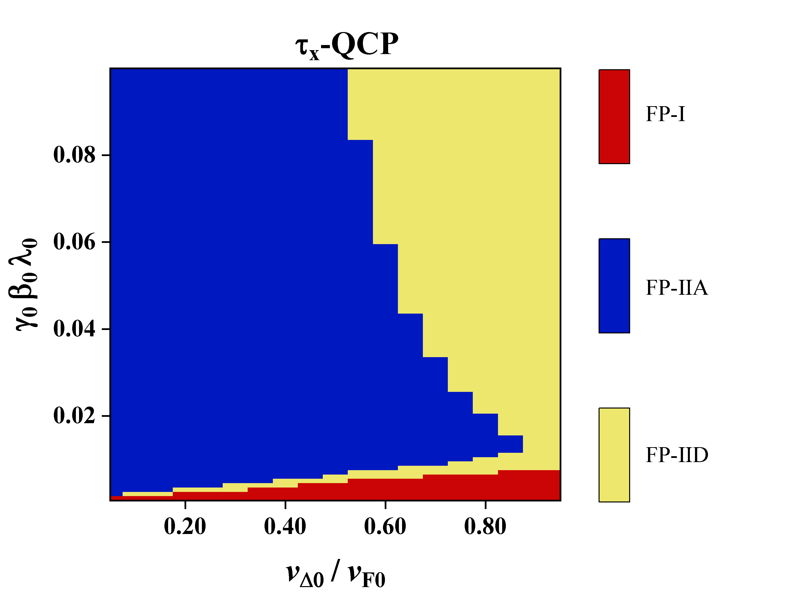
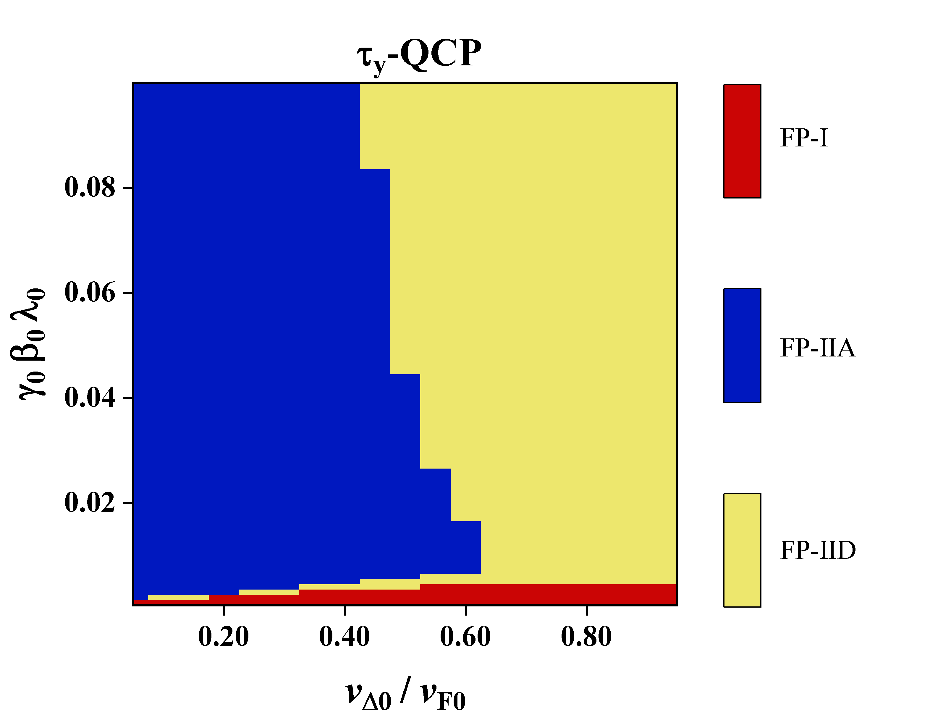
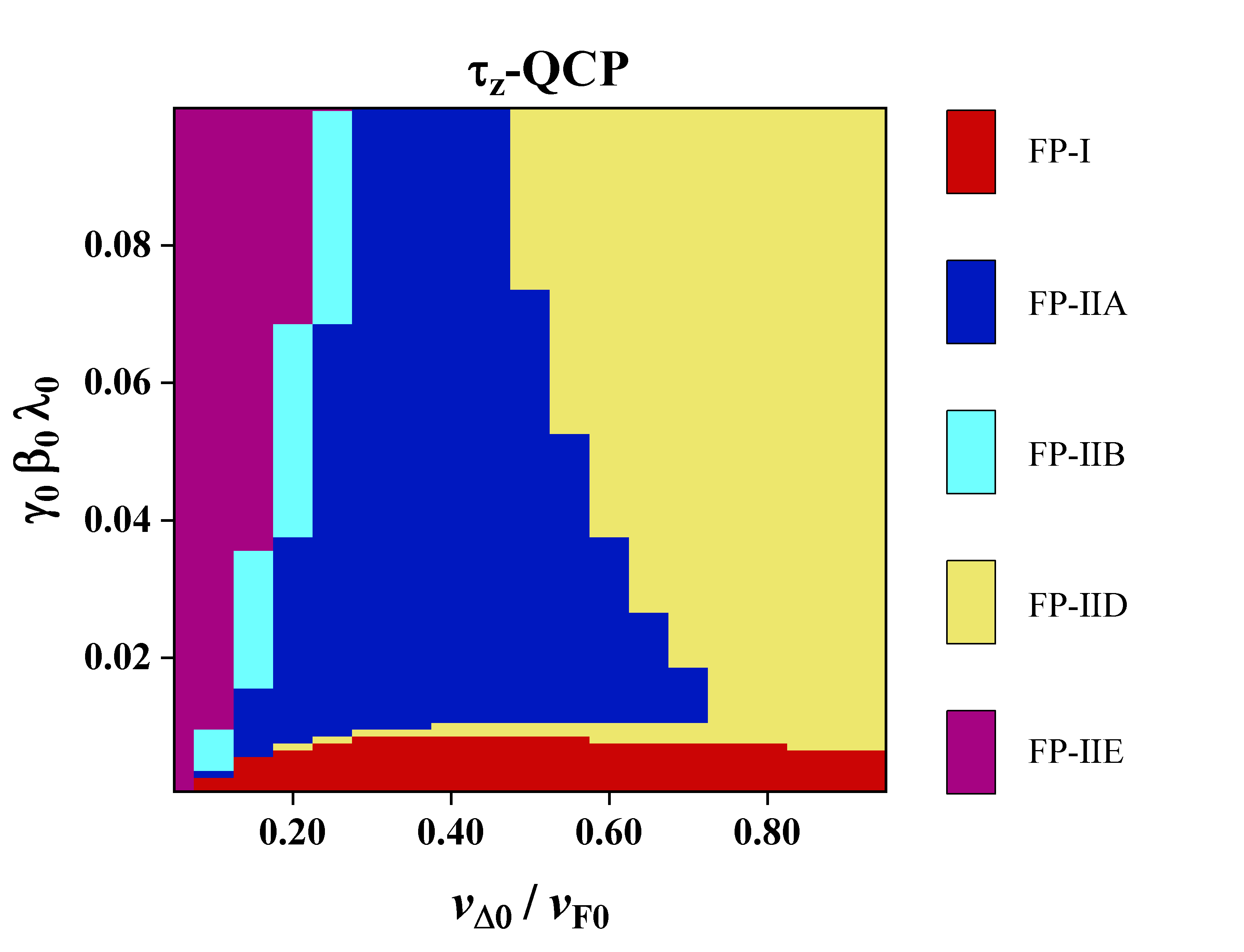
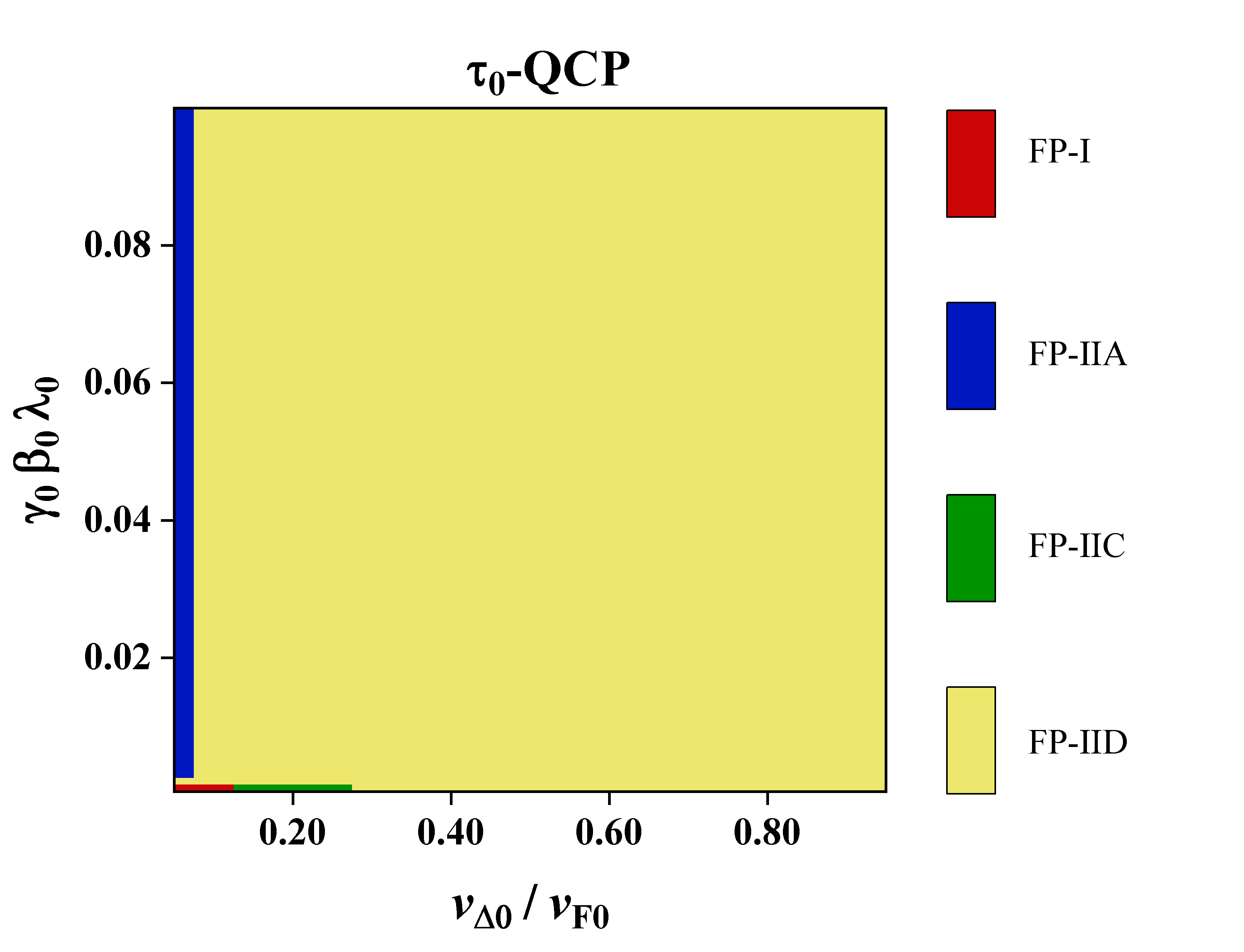
Figure 4: (Color online) The dependence of FPs on the initial condition as the system approaches: (a) $\tau_{x}$-QCP, (b) $\tau_{y}$-QCP, (c) $\tau_{z}$-QCP, and (d)$\tau_{0}$-QCP. The horizontal axis and the vertical axis serve as the initial values of fermion velocities and interaction parameters, respectively.

However, with increasing $\gamma_{0}\beta_{0}\lambda_{0}$, both the interaction parameters and fermion velocities play an important role and the system exhibits distinct FPs around different kinds of QCPs. Considering the $\tau_{x,y}$-QCP, Fig. 4(a) and Fig. 4(b) indicate that these two QCPs share the analogous results. Specifically, besides the Type-I FP, the systems can flow towards either FP-IIA or FP-IID. It can be found that the initial value of fermion velocity anisotropy $v_{\Delta 0}/v_{F0}$ is essential to determine the final FP. Once $v_{\Delta 0}/v_{F0}$ is small, FP-IIA dominates over FP-IID. Instead, the system is always governed by the FP-IID as long as $v_{\Delta 0}/v_{F0}$ is appropriate. For the $\tau_{z}$-QCP, as illustrated in Fig. 4, four candidate FPs, including FP-IIA, FP-IIB, FP-IID, and FP-IIE, emerge with variations of $\gamma_{0}\beta_{0}\lambda_{0}$ and $v_{\Delta 0}/v_{F0}$. In particular, compared to the $\tau_{x,y}$-QCP, the strong fluctuation of order parameter around $\tau_{z}$-QCP induces FP-IIB and FP-IIE in the small $v_{\Delta 0}/v_{F0}$ region. With respect to the $\tau_{0}$-QCP, it is clear from Fig. 4(d) that FP-D predominates among all the FPs observed around $\tau_{x,y,z}$-QCP, with FP-IIA appearing only at very small $v_{\Delta 0}/v_{F0}$. After enlarging the region with the small $\gamma_{0}\beta_{0}\lambda_{0}$ in Fig. 4(d), it is of particular interest to stress that FP-IIC, which is absent in other QCPs, develops within a confined region as depicted in Fig. 5.

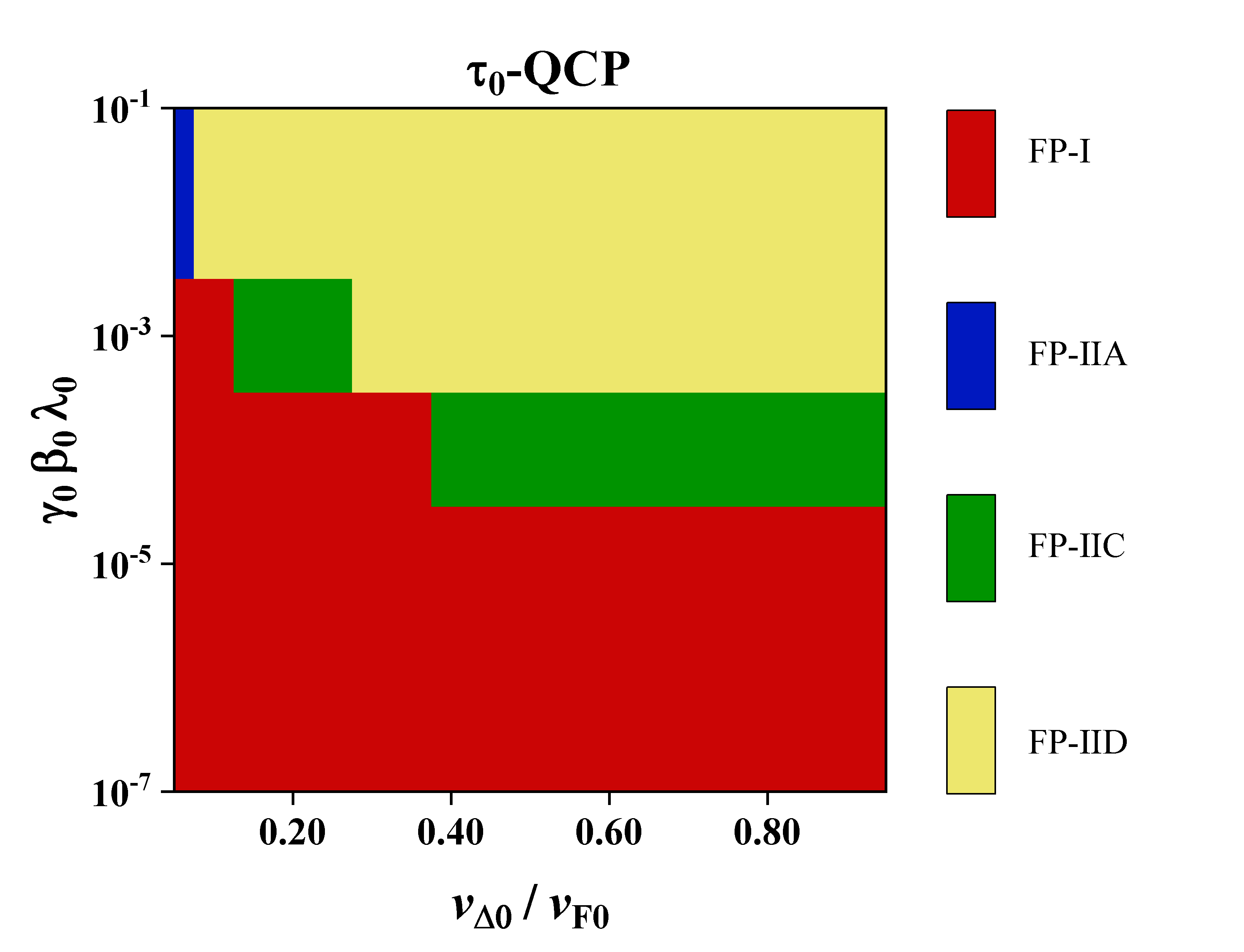
Figure 5: (Color online) The dependence of FPs on the initial condition as the system approaches the $\tau_{0}$-QCP with enlarging the small value regime of Fig. 4(d). The horizontal axis and the vertical axis serve as the initial values of fermion velocities and interaction parameters, respectively.

IV.2.2 Case-General initial conditions

Next, we move to study the impact of Case-General initial conditions on FPs. In order to systematically examine the effects of the initial conditions of interaction parameters, we hereby need to fix the velocities and select several representative values of $v_{\Delta 0}/v_{F0}$. By varying the initial values of $\gamma$, $\beta$ and $\lambda$ independently, careful numerical calculations yield the central results summarized in Fig. 6 and Fig. 7.

As for the $\tau_{x,y,z}$-QCP, Fig. 6 shows that the basic distribution of FPs is similar. Taking the $\tau_{x}$-QCP as an example, as shown in Fig. 6(a)-(c), we realize that for the Case-General, both $\gamma$ and $\beta$ play a dominate role in reshaping the FP, while the $\lambda$ provides much less contributions. Concretely, Fig. 6(a) illustrates that FP-I is dominant when all interaction parameters are less than $10^{-5}$. This is also consistent with the basic tendencies presented in Sec. IV.2.1. However, by increasing $\gamma_{0}$ and choosing an appropriate $\beta_{0}$, FP-IIA can overcome FP-I and become the leading FP. Further, it is worth highlighting that the numerical analysis indicates that the critical energy for FP-I is much lower than that for FP-II, which is crucial to determine the low-energy properties as addressed in following section V.

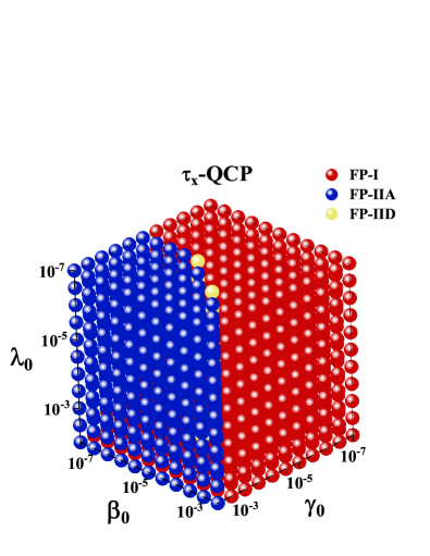
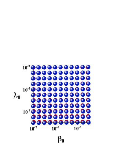
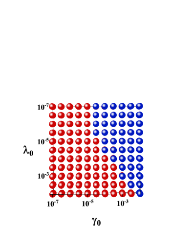
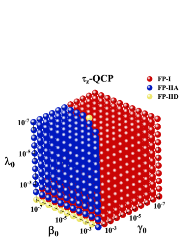
Figure 6: (Color online) The dependence of FPs on three types of interaction parameters $\gamma$, $\beta$ and $\lambda$ for the Case-General as the system approaches: (a)-(c) the $\tau_{x}$-QCP with $v_{\Delta 0}/v_{F0}=0.2$, (d) the $\tau_{x}$-QCP with $v_{\Delta 0}/v_{F0}=0.05$, (e) the $\tau_{y}$-QCP with $v_{\Delta 0}/v_{F0}=0.5$, and (f) the $\tau_{z}$-QCP with $v_{\Delta 0}/v_{F0}=0.8$. Hereby, (b) and (c) correspond to the projections of (a) onto the $\beta_{0}-\lambda_{0}$ plane and the $\gamma_{0}-\lambda_{0}$ plane with a fixed $\gamma_{0}$ and $\beta_{0}$, respectively. These two panels indicate that the interaction parameters $\gamma$ and $\beta$ play a much more significant role than $\lambda$ in determining the FPs.

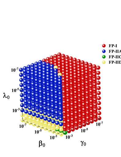
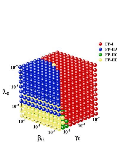
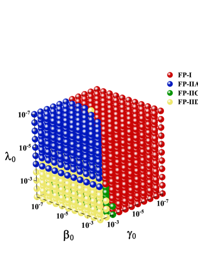
Figure 7: (Color online) The dependence of FPs on three types of interaction parameters $\gamma$, $\beta$ and $\lambda$ for the Case-General as the system approaches the $\tau_{0}$-QCP for distinct initial values of fermion velocities: (a) $v_{\Delta 0}/v_{F0}=0.2$, (b) $v_{\Delta 0}/v_{F0}=0.4$, (c) $v_{\Delta 0}/v_{F0}=0.6$, and (d) $v_{\Delta 0}/v_{F0}=0.8$.

In comparison, more interesting behavior is observed around the $\tau_{0}$-QCP, as depicted in Fig. 7. By fixing $v_{\Delta 0}/v_{F0}$ for several representative values, Fig. 7 shows that the system can flow towards FP-I, FP-IIA, FP-IIC, and FP-IID, depending on the values of $\gamma_{0}$, $\beta_{0}$, and $\lambda_{0}$. Specifically, FP-I is dominant for small values of $\gamma_{0}$. As $\gamma_{0}$ increases, either FP-IIA or FP-IID has an opportunity to be the leading one when both $\lambda_{0}$ and $\beta_{0}$ are appropriately chosen. In addition, FP-IID can appear within a very strict region.

IV.3 Impacts of disorder scatterings

At last, we examine the effects of disorder scatterings on the fermion velocities and critical energy scales of FPs denoted by $l_{c}$. For convenience, the notations RCP, RM, and RGP-$x,z$ are employed to represent the random chemical potential, a random mass, and a random gauge potential addressed in Sec. II.2, respectively.

Numerical analysis shown in Fig. 8(a) indicates that different kinds of disorders exhibit distinct behavior as the energy scale decreases. From Fig. 8(a), one can find that both random mass and random gauge potential decrease and eventually vanish at the lowest-energy scale Wang2011PRB ; Wang2013PRB . In comparison, random chemical potential is marginal to the one-loop level. Accordingly, they give rise to distinct impacts on the fermion velocities and critical energy scales. Considering the fermion velocities, we find that around $\tau_{x}$-QCP shown in Fig. 8(b) they are heavily sensitive to the random chemical potential, which is able to vanish the fermion velocities at a certain finite energy scale. However, both the random mass and random gauge potential provide negligible impacts on the fermion velocities, which gradually vanish at the lowest-energy limit. Similar low-energy behavior is also observed around the $\tau_{z}$-QCP. In sharp contrast, we find that around $\tau_{y,0}$-QCP, the fermion velocities are hardly susceptible to all kinds of disorders.

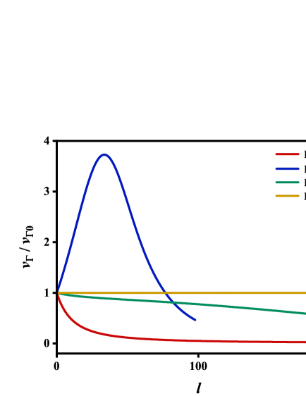
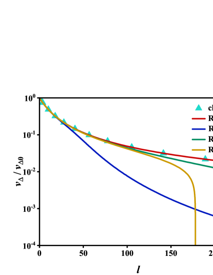
Figure 8: (Color online) Energy-dependent evolutions near the $\tau_{x}$-QCP: (a) the distinct kinds of disorder strengths and (b) fermion velocities under the influence of different sorts of disorders.

In addition, the disorder scatterings may influence the critical energy scales at which the FPs emerge. The RG flow equations (52)-(68) show that the disorder strength $v_{\Gamma}$ does not directly enter the equations of interaction parameters, but it interacts with other parameters by modifying the fermion velocities. For convenience, let us adopt $l_{c}$ to denote the critical energy scale, which is approximately $l_{c}\approx 190$ and $l_{c}\in[3,5]$ for FP-I and FP-II, respectively. Although $v_{\Gamma}$ cannot modify the $l_{c}$ directly, it can influence the fermion velocities, potentially driving them to zero at a finite energy scale denoted by $l^{\prime}_{c}$ when its initial value is appropriate. In this sense, we need to stop the RG equations at $l^{\prime}_{c}$ as fermion velocities become negative at $l>l^{\prime}_{c}$. Therefore, disorder scattering can affect the critical energy scale if $l^{\prime}_{c}<l_{c}$. Given that only the random chemical potential is marginal and could qualitatively contribute to the fermion velocities, we hereby focus exclusively on this type of disorder as schematically illustrated in Fig. 9. Numerical analysis suggests that $l^{\prime}_{c}>l_{c}$ around the $\tau_{y,0}$-QCP (Scenario A) and $l^{\prime\prime}_{c}<l_{c}$ around the $\tau_{x,z}$-QCP (Scenario B). This implies that the random chemical potential can indeed reduce the critical energy scale $l_{c}$ around the $\tau_{x,z}$-QCP.

To recapitulate, we have identified several FPs associated with distinct QCPs and analyzed the effects of disorder around these FPs. Based on these results, we are going to investigate the underlying critical behavior in the vicinity of QCPs.

V Critical behavior induced by the QCPs

Due to the strong quantum fluctuations around the QCPs, all the interactions become coupled as described by flow equations (52)-(68). These coupled interactions give rise to several FPs for distinct kinds FPs of QCPs as presented in Sec. IV, which are accompanied by the critical energy scales. Armed with these, a natural question arises how do these FPs modify the critical behavior nearby the QCPs in Fig. 1. Since the critical temperature is an essential quantity for the superconductors, we hereby place our focus on this very quantity and endeavor to provide a detailed analysis of its critical behavior in the vicinity of the QCPs.

V.1 RG-revised expressions of superfluid density and critical temperature

Beneath the superconducting dome of $d$-wave superconductor, the zero-temperature superfluid ($\rho^{s}(0)$) density exhibits a linear relationship with the doping concentration ($x$), which can be expressed as Orenstein1990PRB ; Hardy1993PRL ; Uemura1989PRL

$$\rho^{s}(0)=\frac{x}{a^{2}},$$ (69)

with $a$ being the lattice spacing constant. At a finite temperature, the normal nodal QPs can be excited from the SC condensate, which provides an inverse feedback to the superfluid density.

At first, let us consider the limit case in which all the interactions and fluctuations are absent. We can obtain the finite-temperature superfluid ($\rho^{s}(T)$) as Lee1997PRL

$$\rho^{s}(T)=\rho^{s}(0)-\rho^{n}(T).$$ (70)

where the normal QPs density takes the form of

$$\rho^{n}(T)=m\frac{2\ln 2}{\pi}\frac{v_{F}}{v_{\Delta}}T,$$ (71)

with $m$ denoting the mass of nodal QP. This therefore gives rise to the critical temperature of SC at $\rho^{s}(T)=0$,

$$T_{c}=\frac{1}{2\ln 2}\frac{v_{\Delta}}{v_{F}}\frac{x}{ma^{2}}.$$ (72)

It is significant to emphasize that the fermion velocities thereby are some constants, which are equivalent to the initial values $v_{\Delta 0},v_{F0}$ mentioned in Sec. IV.

Next, we switch on the interactions and quantum fluctuations in the vicinity of the potential QCP shown in Fig. 1. As presented in Sec. III, all the interaction parameters are closely coupled under the control of the RG Eqs. (52)-(68). This accordingly renormalizes the fermion velocities and make them energy-dependent from $v_{\Delta 0},v_{F0}$ to $v_{\Delta}(k),v_{F}(k)$ that are dictated by the RG evolutions. On the basis of these considerations, the normal QPs density is renormalized and recast to Lee1997PRL ; Durst2000PRB ; Liu2012PRB

$$\rho_{R}^{n}(T)=\frac{4m}{k_{B}T}\left[\int_{0}^{\Lambda_{c}}\frac{d^{2}\mathbf{k}}{(2\pi)^{2}}\frac{v_{F}^{2}(\mathbf{k})e^{\sqrt{v_{F}^{2}(\mathbf{k})k_{x}^{2}+v_{\Delta}^{2}(\mathbf{k})k_{y}^{2}}/k_{B}T}}{\left(1+e^{\sqrt{v_{F}^{2}(\mathbf{k})k_{x}^{2}+v_{\Delta}^{2}(\mathbf{k})k_{y}^{2}}/k_{B}T}\right)^{2}}+\int_{\Lambda_{c}}^{\infty}\Bigl{(}v_{F,\Delta}(\mathbf{k})\rightarrow v_{F,\Delta}(l_{c})\Bigr{)}\right],$$ (73)

where $k_{B}$ denotes the Boltzmann constant. Here, $\Lambda_{c}$ represents the critical energy and is associated with $l_{c}$ for a given FP. Several clarifications are necessary at this point. As aforementioned in Sec. IV.1, the RG equations are no longer valid beyond $l_{c}$. Therefore, we divide the whole energy regime into two regions, namely $l\in[0,l_{c})$ and $l\geq l_{c}$. In other words, for $l\in[0,l_{c})$, the fermion velocities are energy-dependent due to the RG flow, which fully captures the effects of quantum fluctuations. In contrast, for $l\geq l_{c}$, we go beyond the mean-field approach, where the fermion velocities are treated as constants (i.e., $v_{\Delta 0}$ and $v_{F0}$), but adopt the RG-renormalized mean-field method, in which these constants $v_{\Delta 0}$ and $v_{F0}$ are replaced by the $v_{\Delta}(l_{c})$ and $v_{F}(l_{c})$, which are modified by the quantum fluctuations at the energy scale $l_{c}$ Metzner2000PRL ; Reiss2007PRB ; Wang-EM2014PRB . As a result, the presence of quantum fluctuations renormalizes the superfluid density (70) to the following form,

$$\rho_{R}^{s}(T)=\rho^{s}(0)-\rho_{R}^{n}(T),$$ (74)

from which the renormalized critical temperature ($T^{\prime}_{c}$) can be obtained by taking $\rho_{R}^{s}(T^{\prime}_{c})=0$.

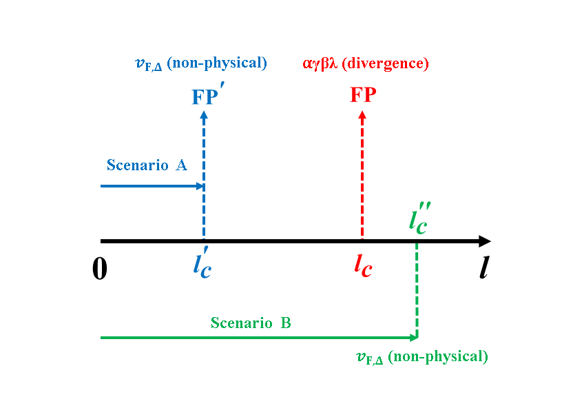
Figure 9: (Color online) Schematic illustrations of distinct kinds of low-energy fates as approaching the QCPs. The red one serves as the clean-limit case, in which the FP associated with divergence of interaction parameters is determined at $l=l_{c}$. In the presence of the random chemical potential, there exist two potential scenarios, namely Scenario A (blue) and Scenario B (green).

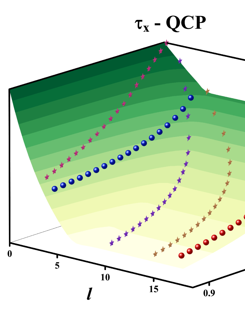
Figure 10: (Color online) The tendencies of the renormalized critical temperature $T^{\prime}_{c}$ relative to the initial critical temperature $T_{c}$ nearby distinct FPs as approaching the $\tau_{x}$-QCP. $T^{\prime}_{c}/T_{c}$ depend upon the energy scales ($l$) and the initial value of fermion velocities ($v_{\Delta 0}/v_{F0}$) in the presence of random chemical potential.

V.2 Numerical results for the renormalized critical temperature

With all above on hand, we are now in a proper position to examine the behavior of critical temperature around different kinds of QCPs. Reading from Eq. (73) and Eq. (74), we can infer that there exist two significant items that are largely associated with the critical temperature. One is the initial values of fermion velocities at $l=0$ and the other is the critical energy scale denoted by $l_{c}$ of the FP. In particular, learning from Sec. IV around the QCPs, we find that the critical energy scale $l_{c}$ is closely related to the type of FP.

After performing the detailed numerical analysis of the RG equations (52)-(68) and the renormalized superfluid density (73)-(74), we examine the impacts of QCPs as shown in Fig. 1 on the critical temperature. The results are presented in Fig. 10-11 for different kinds of FPs. These figures clearly illustrate the dependence of the renormalized critical temperature $T^{\prime}_{c}/T_{c}$ on the initial ratio of fermion velocities $v_{\Delta 0}/v_{F0}$ and the critical energy scale $l_{c}$ around distinct QCPs. Here, $T^{\prime}_{c}$ and $T_{c}$ serve as the renormalized and non-interacting critical temperatures, respectively.

At the outset, we consider the $\tau_{x}$-QCP. One can find from Fig. 10 that the quantum fluctuations cause a pronounced decrease in the critical temperature for both FP-I and FP-II, as discussed in Sec. IV.1. Tuning up the $v_{\Delta 0}/v_{F0}$ is prone to decreasing the critical temperature. In addition, one can notice that $T^{\prime}_{c}$ decreases a little more sharply as the system approaches FP-I compared to FP-II. Further, we study the effects of random chemical potential which is marginal and has an opportunity to provide nontrivial corrections as explained in Sec. IV.3. As shown in Fig. 9, the occurrence of Scenario A or Scenario B depends on both the initial disorder strength $v_{\Gamma 0}$ and the ratio $v_{\Delta 0}/v_{F0}$. For the FP-I, once $v_{\Gamma 0}$ is suitable, the system always transitions to Scenario A, leading to a slight increase in $T^{\prime}_{c}$ compared to the clean limit case. For FP-II, Scenario B is preferred under most conditions. However, Scenario A can also be realized when both $v_{\Delta 0}/v_{F}$ and $v_{\Gamma 0}$ are appropriately chosen, such as $v_{\Gamma_{0}}=0.3$ and $v_{\Delta 0}/v_{F0}\textless 0.1$. This accordingly indicates that random chemical potential plays an important role around the $\tau_{x}$-QCP.

Subsequently, let us move to the $\tau_{y}$-QCP and $\tau_{0}$-QCP. We find that Scenario-A in Fig. 9 triggered by disorder scatterings cannot be realized for these two QCPs. This implies that our analysis should focus on the clean limit case. In sharp contrast to the $\tau_{x}$-QCP, nearby the $\tau_{y}$-QCP, Fig. 11(a) shows that the renormalized critical temperature $T^{\prime}_{c}$ for both FP-I and FP-II increases and would exhibit a peak at $x_{c}$ in Fig. 1 induced by the quantum fluctuations. Particularly, $T^{\prime}_{c}$ is sensitive to the ratio $v_{\Delta 0}/v_{F0}$, reaching its maximum at $v_{\Delta 0}/v_{F0}\approx 0.25$ and gradually decreasing as $v_{\Delta 0}/v_{F0}$ either increases or decreases. In addition, $T^{\prime}_{c}$ for FP-I is slightly higher than for FP-II. As we approach the $\tau_{0}$-QCP, the renormalized critical temperature becomes more sensitive to the types of FPs, but less sensitive to the initial values of fermion velocities. These are remarkable different from those around $\tau_{x}$-QCP and $\tau_{y}$-QCP. Fig. 11(b) manifests that $T^{\prime}_{c}$ is slightly smaller than the non-interacting critical temperature $T_{c}$ in the absence of quantum fluctuations. However, when FP-I is accessed, $T^{\prime}_{c}$ undergoes a significant dip, reaching a value of $T^{\prime}_{c}/T_{c}=0.72$.

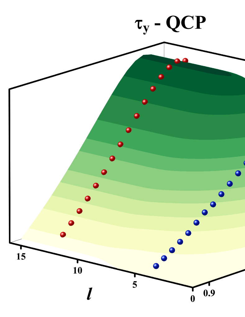
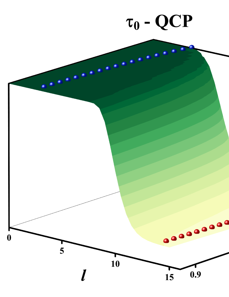
Figure 11: (Color online) The tendencies of the renormalized critical temperature $T^{\prime}_{c}$ relative to the initial critical temperature $T_{c}$ nearby distinct FPs as approaching (a) the $\tau_{y}$-QCP and (b) the $\tau_{0}$-QCP. $T^{\prime}_{c}/T_{c}$ depend upon the energy scales ($l$) and the initial value of fermion velocities ($v_{\Delta 0}/v_{F0}$) in the presence of random chemical potential.

At last, we offer several comments on the $\tau_{z}$-QCP. By performing a similar numerical analysis as done for the $\tau_{x,y,0}$-QCP, we notice that the renormalized temperature $T^{\prime}_{c}$ around the $\tau_{z}$-QCP is heavily increased for all initial values of fermion velocities. In particular, $T^{\prime}_{c}/T_{c}$ exceeds $10$ at $v_{\Delta 0}/v_{F0}=0.1$. Such a high critical temperature has not yet been reported for the $d$-wave superconductors Lee2006RMP ; Fradkin2015RMP ; Keimer2008Science ; Orenstein2000Science ; Bozovic2016Nature ; Phiillips2022Science ; Ramakrishnan2025 . Under this circumstance, although all four kinds of QCPs are allowed from a symmetry perspective, we argue that the $\tau_{z}$-QCP can hardly be realized from the physical perspective but instead all the other three QCPs own the opportunity to be the candidate QCP.

To be brief, the critical temperature of $d$-wave superconductors would be considerably modified by the quantum fluctuations around the QCPs. Depending on the type of QCP, the critical temperature can either increase (around the $\tau_{y}$-QCP) or decrease (around the $\tau_{x,0}$-QCP). The exact value of $T^{\prime}_{c}$ is associated with the sorts of FPs and initial values of fermion velocities.

VI Summary

In summary, we systematically investigate a quantum phase transition (QPT) beneath the superconducting dome of a $d$-wave cuprate superconductor. This transition evolves from a pure $d$-wave superconducting state to a mixed state characterized by $d$-wave superconductivity coexisting with an additional order parameter $X$, as illustrated in Fig. 1. For completeness, we examine four potential quantum critical points (QCPs) associated with this QPT: $\tau_{0}$-Type, $\tau_{x}$-Type, $\tau_{y}$-Type, and $\tau_{z}$-Type QCPs Vojta2000PRL ; Vojta2000PRB ; Wang2013PRB . To equally account for distinct degrees of freedom near these QCPs, we employ the RG approach Shankar1994RMP ; Wilson1975RMP ; Polchinski1992 , which allows us to derive the coupled, energy-dependent flow equations for all relevant interaction parameters within our effective theory. After analyzing these equations, several critical phenomena near the QCPs are induced due to strong quantum fluctuations.

We begin by performing a numerical analysis of the coupled RG flow equations (52)-(68). Our results indicate that the overall behavior of the interaction parameters is governed by a set of fixed points (FPs) located at $l=l_{c}$, which are closely tied to the low-energy critical behavior of the system Maiti2010PRB ; Vojta2003RPP ; Roy2018PRX ; Wang2017QBCP ; Vafek2012PRB ; Vafek2014PRB ; Wang2020PRB ; Chubukov2012ARCMP ; Chubukov2016PRX ; Nandkishore2012NP ; Wang2020NPB . At the clean limit, varying the initial conditions leads to the emergence of two distinct types of FPs. FP-I is characterized by the divergence of the quadratic parameter, which remains largely unaffected by other interaction parameters. In contrast, FP-II is dominated by the cubic and quartic interaction parameters. Besides, since the specific values of FP-II are highly sensitive to the initial conditions, as illustrated in Fig. 3, it further divides into five subclasses, including FP-IIA, FP-IIB, FP-IIC, FP-IID, and FP-IIE. To proceed, we introduce three types of disorders and examine the effects of fermion-disorder coupling (37) on the stability of these FPs. Numerical analysis demonstrates that both random mass and random gauge potential provide negligible impacts on FPs for all QCPs. However, the random chemical potential significantly influences either the fermion velocities or the critical energy scales. Specifically, it tends to reduce the critical energy scale $l_{c}$ near the $\tau_{x,z}$-QCP, as shown in Fig. 9.

Next, we carefully investigate the impacts of strong quantum fluctuations on the critical temperature as the system approaches the FPs for all potential QCPs in Fig. 1. For the $\tau_{x}$-QCP, the critical temperature is significantly suppressed for both FP-I and FP-II, as depicted in Fig. 10. In particular, the critical temperature gradually decreases as $v_{\Delta 0}/v_{F0}$ increases and it decreases a little more sharply as approaching FP-I compared to FP-II. In addition, the random chemical potential can lead to either Scenario A or Scenario B in Fig. 9 as long as the initial conditions are appropriately tuned around the $\tau_{x}$-QCP. In particular, the critical temperature decreases gradually with increasing $v_{\Delta 0}/v_{F0}$, exhibiting a slightly sharper decline near FP-I than near FP-II. With respect to the $\tau_{y}$-QCP and $\tau_{0}$-QCP, the critical temperature, as depicted in Fig. 11, is primarily determined by the ratio $v_{\Delta 0}/v_{F0}$ and the critical energy scale $l_{c}$, while remaining largely insensitive to disorder scattering. This is because Scenario A in Fig. 9 cannot be realized in these cases. Notably, for the $\tau_{y}$-QCP, the critical temperature increases and exhibits a strong dependence on the fermion velocities, reaching a distinct peak at $v_{\Delta 0}/v_{F0}\sim 0.25$. In comparison, for the $\tau_{0}$-QCP, the critical temperature becomes more sensitive to the type of FP but less sensitive to the initial values of the fermion velocities. In this sense, the critical temperature is slightly lower and undergoes a significant dip for FP-I and FP-II, respectively.

Considering the $\tau_{z}$-QCP, direct numerical analysis indicates that the critical temperature can be significantly enhanced for all initial values of the fermion velocities. However, this enhancement lies well beyond the range of critical temperatures $T_{c}$ typically observed in $d$-wave superconductors Lee2006RMP ; Fradkin2015RMP ; Keimer2008Science ; Orenstein2000Science ; Bozovic2016Nature ; Phiillips2022Science ; Ramakrishnan2025 . Consequently, we infer that such a QCP is unlikely to be physically realizable. This analysis of critical behavior provides a strategy to exclude the $\tau_{z}$-QCP, as illustrated in Fig. 1, while supporting the potential existence of the other three QCPs. We hope that these findings will contribute to clarifying the critical behavior of $d$-wave superconductors and improve our understanding of these materials and related systems in the future.

Appendix A One-loop corrections

On the basis of the total phenomenological effective theory around the QCP (38), we obtain the tree level and one-loop Feynman diagrams as shown in Figs. 12-18. After performing long but straightforward algebraic calculations Shankar1994RMP ; Kim2008PRB ; Huh2008PRB ; She2010PRB ; She2015PRB ; Wang2011PRB ; Wang2013PRB ; Wang2014PRD ; Wang2015PRB ; Wang2017PRB ; Wang2017QBCP ; Vafek2012PRB ; Vafek2014PRB ; Wang2022SST , we derive all the one-loop corrections as follows,

Figure 12: Free propagators for distinct kinds of fields: (a) $\Psi$, (b) $\phi$, (c) $h$, (d) $\eta$, and (e) $A$.

Figure 13: Tree-level vertices: (a) $\Psi^{2}\phi$; (b) $\Psi^{2}\Gamma$; (c) $h^{3}$; (d) $\eta^{2}h$; (e) $\phi^{2}h$; (f) $h^{4}$; (g) $h^{2}\eta^{2}$; (h) $h^{2}\phi^{2}$; (i) $\eta^{4}$; (j) $\phi^{4}$; (k) $\eta^{2}\phi^{2}$.

Figure 14: One-loop corrections to the propagators of fields: ($\rm{a_{1}}$)-($\rm{a_{2}}$) for $\Psi$, ($\rm{b_{1}}$)-($\rm{b_{5}}$) for $\phi$, and ($\rm{c_{1}}$)-($\rm{c_{6}}$) for $h$ due to the ordering competition.

Figure 15: One-loop corrections to the fermion-disorder coupling for($\rm{a_{1}}$)-($\rm{a_{2}}$) and the Yukawa coupling between the QPs and $X$-state order parameter for($\rm{b_{1}}$)-($\rm{b_{2}}$).

Figure 16: One-loop corrections to $\gamma_{h}$ ($\rm{a_{1}}$)-($\rm{a_{4}}$), $\gamma_{\eta h}$ ($\rm{b_{1}}$)-($\rm{b_{4}}$), and $\gamma_{\phi h}$ ($\rm{c_{1}}$)-($\rm{c_{4}}$) due to the ordering competition.

Figure 17: One-loop corrections to $\beta_{\phi}$ ($\rm{a_{1}}$)-($\rm{a_{4}}$), $\beta_{\eta}$ ($\rm{b_{1}}$)-($\rm{b_{4}}$), and $\beta_{\phi}$ ($\rm{c_{1}}$)-($\rm{c_{4}}$) due to the ordering competition.

Figure 18: One-loop corrections to $\lambda_{\eta h}$ ($\rm{a_{1}}$)-($\rm{a_{6}}$), $\lambda_{h\phi}$ ($\rm{b_{1}}$)-($\rm{b_{6}}$), and $\lambda_{\eta\phi}$ ($\rm{c_{1}}$)-($\rm{c_{6}}$) due to the ordering competition.

$$\Delta S^{\Psi} = -2\lambda_{0}^{2}(\mathcal{A}^{i}_{1}(-i\omega)+\mathcal{A}^{i}_{2}v_{F}k_{x}\tau^{z}+\mathcal{A}^{i}_{3}v_{\Delta}k_{y}\tau^{x})l-2C_{g}i\omega l,$$ (75)

$$\Delta S^{\alpha_{h}} = \frac{1}{2\pi^{2}}\Big{[}-3\gamma_{h}^{2}-\gamma_{\eta h}^{2}-\frac{64}{\pi}\gamma_{\phi h}^{2}v_{F}^{2}v_{\Delta}^{2}\mathcal{F}_{2}^{i}(\theta,\varphi)+\frac{3}{4}\beta_{h}(1-2\alpha_{h})+\frac{1}{2}\lambda_{\eta h}$$ (76)

$$+\frac{2v_{F}v_{\Delta}}{\pi}\lambda_{h\phi}\mathcal{F}_{1}^{i}(\theta,\varphi)\bigg{]}l,$$

$$\Delta S^{v_{\Gamma}} = 4v_{\Gamma}\left[(\mathcal{A}^{i}_{1}-3C_{g})I+(\mathcal{A}^{i}_{1}+\mathcal{A}^{i}_{2}-\mathcal{A}^{i}_{3}+3C_{g})\tau^{y}+\mathcal{A}^{i}_{3}\tau^{x}+\mathcal{A}^{i}_{2}\tau^{z}\right]l,$$ (77)

$$\Delta S^{\gamma_{h}} = \frac{1}{4\pi^{2}}\bigg{[}-8\gamma_{h}^{3}(1-6\alpha_{h})+\beta_{h}\gamma_{h}(1-4\alpha_{h})-\lambda_{\eta h}\gamma_{\eta h}-\frac{\lambda_{h\phi}\gamma_{\phi h}}{2\pi}(16v_{F}v_{\Delta})^{2}\mathcal{F}^{i}_{2}(\theta,\varphi)\bigg{]}l,$$ (78)

$$\Delta S^{\gamma_{\eta h}} = \frac{1}{4\pi^{2}}\bigg{[}-2\gamma_{\eta h}^{3}(1-2\alpha_{h})+\beta_{\eta}\gamma_{\eta h}-2\lambda_{\eta h}\gamma_{h}(1-4\alpha_{h})-\frac{\lambda_{\eta\phi}\gamma_{\phi h}}{2\pi}(16v_{F}v_{\Delta})^{2}\mathcal{F}^{i}_{2}(\theta,\varphi)\bigg{]}l,$$ (79)

$$\Delta S^{\gamma_{\phi h}} = \frac{1}{2\pi^{2}}\bigg{[}-\frac{\gamma_{\phi h}^{3}}{4\pi}(1-2\alpha_{h})(16v_{F}v_{\Delta})^{2}\mathcal{F}^{i}_{2}(\theta,\varphi)-\lambda_{h\phi}\gamma_{h}(1-4\alpha_{h})-\lambda_{\eta\phi}\gamma_{\eta h}$$ (80)

$$+\frac{\beta_{\phi}\gamma_{\phi h}}{8\pi}(16v_{F}v_{\Delta})^{2}\mathcal{F}^{i}_{2}(\theta,\varphi)\bigg{]}l,$$

$$\Delta S^{\beta_{h}} = \frac{1}{4\pi^{2}}\bigg{[}-4\beta_{h}\gamma_{h}^{2}(1-6\alpha_{h})+\frac{\beta_{h}^{2}}{2}(1-4\alpha_{h})-2\lambda_{\eta h}^{2}-\frac{\lambda_{h\phi}^{2}}{2\pi}(16v_{F}v_{\Delta})^{2}\mathcal{F}^{i}_{2}(\theta,\varphi)\bigg{]}l,$$ (81)

$$\Delta S^{\beta_{\eta}} = \frac{1}{4\pi^{2}}\bigg{[}-\beta_{\eta}\gamma_{\eta h}^{2}(1-2\alpha_{h})+\frac{1}{2}\beta_{\eta}^{2}-2\lambda_{\eta h}^{2}(1-4\alpha_{h})-\frac{\lambda_{h\phi}^{2}}{2\pi}(16v_{F}v_{\Delta})^{2}\mathcal{F}^{i}_{2}(\theta,\varphi)\bigg{]}l,$$ (82)

$$\Delta S^{\beta_{\phi}} = \frac{1}{4\pi^{2}}\bigg{[}-\frac{\beta_{\phi}\gamma_{\phi h}^{2}}{4\pi}(1-2\alpha_{h})(16v_{F}v_{\Delta})^{2}\mathcal{F}^{i}_{2}(\theta,\varphi)-2\lambda_{\phi h}^{2}(1-4\alpha_{h})$$ (83)

$$-2\lambda_{\eta\phi}^{2}+\frac{\beta_{\phi}^{2}}{8\pi}(16v_{F}v_{\Delta})^{2}\mathcal{F}^{i}_{2}(\theta,\varphi)\bigg{]}l$$

$$\Delta S^{\lambda_{\eta h}} = \frac{1}{2\pi^{2}}\bigg{[}-4\lambda_{\eta h}\gamma_{h}^{2}(1-6\alpha_{h})+\frac{\lambda_{\eta h}^{2}}{2}(1-2\alpha_{h})+\frac{\beta_{h}\lambda_{\eta h}}{2}(1-4\alpha_{h})+\frac{\beta_{h}\lambda_{\eta h}}{2}$$ (84)

$$-4\lambda_{\eta h}\gamma_{\eta h}^{2}(1-2\alpha_{h})-\frac{\lambda_{\eta\phi}\lambda_{h\phi}}{4\pi}(16v_{F}v_{\Delta})^{2}\mathcal{F}^{i}_{2}(\theta,\varphi)\bigg{]}l,$$

$$\Delta S^{\lambda_{h\phi}} = \frac{1}{2\pi^{2}}\bigg{[}-4\lambda_{h\phi}\gamma_{h}^{2}(1-6\alpha_{h})+\frac{\lambda_{h\phi}^{2}}{8\pi}(1-2\alpha_{h})(16v_{F}v_{\Delta})\mathcal{F}_{1}^{i}(\theta,\varphi)+\frac{\beta_{\phi}\lambda_{h\phi}}{8\pi}(16v_{F}v_{\Delta})^{2}\mathcal{F}_{2}^{i}(\theta,\varphi)-\lambda_{\eta h}\lambda_{\eta\phi}$$ (85)

$$+\frac{\beta_{h}\lambda_{h\phi}}{2}(1-4\alpha_{h})-\frac{1}{4\pi}\lambda_{h\phi}\gamma_{\phi h}^{2}(1-2\alpha_{h})(16v_{F}v_{\Delta})^{2}\mathcal{F}_{2}^{i}(\theta,\varphi)\bigg{]}l,$$

$$\Delta S^{\lambda_{\eta\phi}} = \frac{1}{4\pi^{2}}\bigg{[}-2\lambda_{\eta\phi}\gamma_{\eta h}^{2}(1-2\alpha_{h})-\frac{\lambda_{\eta\phi}\gamma_{\phi h}^{2}}{2\pi}(1-2\alpha_{h})(16v_{F}v_{\Delta})^{2}\mathcal{F}^{i}_{2}(\theta,\varphi)-2\lambda_{\eta\phi}\lambda_{h\phi}(1-4\alpha_{h})+\beta_{\eta}\lambda_{\eta\phi}$$ (86)

$$+\frac{\beta_{\phi}\lambda_{\eta\phi}}{4\pi}(16v_{F}v_{\Delta})^{2}\mathcal{F}^{i}_{2}(\theta,\varphi)+\frac{\lambda_{\eta\phi}^{2}}{4\pi}(16v_{F}v_{\Delta})\mathcal{F}^{i}_{1}(\theta,\varphi)\bigg{]}l.$$

Hereby, the superscripts $i=\tau_{x,y,z,0}$ of the related coefficients $\mathcal{A}^{i}_{1,2,3}$ and $\mathcal{F}^{i}_{1,2}$ are adopted to specify the type $\tau_{x,y,z,0}-$QCP. Specifically, they are denominated as

$$\mathcal{A}^{\tau_{x}}_{1} \equiv \frac{2(v_{\Delta}/v_{F})}{N_{f}\pi^{3}}\int_{-\infty}^{\infty}dx\int_{0}^{2\pi}d\theta\frac{x^{2}-\cos^{2}\theta-(v_{\Delta}/v_{F})^{2}\sin^{2}\theta}{[x^{2}+\cos^{2}\theta+(v_{\Delta}/v_{F})^{2}\sin^{2}\theta]^{2}}\mathcal{G}_{x}(x,\theta),$$ (87)

$$\mathcal{A}^{\tau_{x}}_{2} \equiv \frac{2(v_{\Delta}/v_{F})}{N_{f}\pi^{3}}\int_{-\infty}^{\infty}dx\int_{0}^{2\pi}d\theta\frac{-x^{2}+\cos^{2}\theta-(v_{\Delta}/v_{F})^{2}\sin^{2}\theta}{[x^{2}+\cos^{2}\theta+(v_{\Delta}/v_{F})^{2}\sin^{2}\theta]^{2}}\mathcal{G}_{x}(x,\theta),$$ (88)

$$\mathcal{A}^{\tau_{x}}_{3} \equiv \frac{2(v_{\Delta}/v_{F})}{N_{f}\pi^{3}}\int_{-\infty}^{\infty}dx\int_{0}^{2\pi}d\theta\frac{x^{2}+\cos^{2}\theta-(v_{\Delta}/v_{F})^{2}\sin^{2}\theta}{[x^{2}+\cos^{2}\theta+(v_{\Delta}/v_{F})^{2}\sin^{2}\theta]^{2}}\mathcal{G}_{x}(x,\theta),$$ (89)

$$\mathcal{R}^{\tau_{x}} \equiv \frac{2(v_{\Delta}/v_{F})}{N_{f}\pi^{3}}\int^{\infty}_{-\infty}dx\int_{0}^{2\pi}d\theta\frac{-x^{2}-\cos^{2}\theta+(v_{\Delta}/v_{F})^{2}\sin\theta^{2}}{[x^{2}+\cos^{2}\theta+(v_{\Delta}/v_{F})^{2}\sin^{2}\theta]^{2}}\mathcal{G}_{x}(x,\theta),$$ (90)

$$\mathcal{G}_{x}^{-1}(x,\theta) \equiv \frac{x^{2}+\cos^{2}\theta}{\sqrt{x^{2}+\cos^{2}\theta+(v_{\Delta}/v_{F})^{2}\sin^{2}\theta}}+\frac{x^{2}+\sin^{2}\theta}{\sqrt{x^{2}+\sin^{2}\theta+(v_{\Delta}/v_{F})^{2}\cos^{2}\theta}},$$ (91)

$$\mathcal{F}^{\tau_{x}}(\theta,\varphi) \equiv \frac{\cos^{2}\theta+v_{F}^{2}\cos^{2}\varphi\sin^{2}\theta}{\sqrt{\cos^{2}\theta+v_{F}^{2}\cos^{2}\varphi\sin^{2}\theta+v_{\Delta}^{2}\sin^{2}\varphi\sin^{2}\theta}}+\frac{\cos^{2}\theta+v_{F}^{2}\sin^{2}\varphi\sin^{2}\theta}{\sqrt{\cos^{2}\theta+v_{F}^{2}\sin^{2}\varphi\sin^{2}\theta+v_{\Delta}^{2}\cos^{2}\varphi\sin^{2}\theta}},$$ (92)

$$\mathcal{F}^{\tau_{x}}_{1}(\theta,\varphi) \equiv \int_{0}^{\pi}d\theta\int_{0}^{2\pi}d\varphi\frac{\sin\theta}{\mathcal{F}^{\tau_{x}}(\theta,\varphi)},$$ (93)

$$\mathcal{F}^{\tau_{x}}_{2}(\theta,\varphi) \equiv \int_{0}^{\pi}d\theta\int_{0}^{2\pi}d\varphi\frac{\sin\theta}{[\mathcal{F}^{\tau_{x}}(\theta,\varphi)]^{2}}.$$ (94)

for the type $\tau_{x}$-QCP,

$$\mathcal{A}^{\tau_{y}}_{1} \equiv \frac{2(v_{\Delta}/v_{F})}{N_{f}\pi^{3}}\int_{-\infty}^{\infty}dx\int_{0}^{2\pi}d\theta\frac{x^{2}-\cos^{2}\theta-(v_{\Delta}/v_{F})^{2}\sin^{2}\theta}{[x^{2}+\cos^{2}\theta+(v_{\Delta}/v_{F})^{2}\sin^{2}\theta]^{2}}\mathcal{G}_{y}(x,\theta),$$ (95)

$$\mathcal{A}^{\tau_{y}}_{2} \equiv \frac{2(v_{\Delta}/v_{F})}{N_{f}\pi^{3}}\int_{-\infty}^{\infty}dx\int_{0}^{2\pi}d\theta\frac{-x^{2}+\cos^{2}\theta-(v_{\Delta}/v_{F})^{2}\sin^{2}\theta}{[x^{2}+\cos^{2}\theta+(v_{\Delta}/v_{F})^{2}\sin^{2}\theta]^{2}}\mathcal{G}_{y}(x,\theta),$$ (96)

$$\mathcal{A}^{\tau_{y}}_{3} \equiv \frac{2(v_{\Delta}/v_{F})}{N_{f}\pi^{3}}\int_{-\infty}^{\infty}dx\int_{0}^{2\pi}d\theta\frac{-x^{2}-\cos^{2}\theta+(v_{\Delta}/v_{F})^{2}\sin^{2}\theta}{[x^{2}+\cos^{2}\theta+(v_{\Delta}/v_{F})^{2}\sin^{2}\theta]^{2}}\mathcal{G}_{y}(x,\theta),$$ (97)

$$\mathcal{R}^{\tau_{y}} \equiv \frac{2(v_{\Delta}/v_{F})}{N_{f}\pi^{3}}\int^{\infty}_{-\infty}dx\int_{0}^{2\pi}d\theta\frac{-x^{2}-\cos^{2}\theta+(v_{\Delta}/v_{F})^{2}\sin\theta^{2}}{[x^{2}+\cos^{2}\theta+(v_{\Delta}/v_{F})^{2}\sin^{2}\theta]^{2}}\mathcal{G}_{y}(x,\theta),$$ (98)

$$\mathcal{G}_{y}^{-1}(x,\theta) \equiv \sqrt{x^{2}+\cos^{2}\theta+(v_{\Delta}/v_{F})^{2}\sin^{2}\theta}+\sqrt{x^{2}+\sin^{2}\theta+(v_{\Delta}/v_{F})^{2}\cos^{2}\theta},$$ (99)

$$\mathcal{F}^{\tau_{y}}(\theta,\varphi) \equiv \sqrt{\cos^{2}\theta+v_{F}^{2}\cos^{2}\varphi\sin^{2}\theta+v_{\Delta}^{2}\sin^{2}\varphi\sin^{2}\theta}+\sqrt{\cos^{2}\theta+v_{F}^{2}\sin^{2}\varphi\sin^{2}\theta+v_{\Delta}^{2}\cos^{2}\varphi\sin^{2}\theta},$$ (100)

$$\mathcal{F}^{\tau_{y}}_{1}(\theta,\varphi) \equiv \int_{0}^{\pi}d\theta\int_{0}^{2\pi}d\varphi\frac{\sin\theta}{\mathcal{F}^{\tau_{y}}(\theta,\varphi)},$$ (101)

$$\mathcal{F}^{\tau_{y}}_{2}(\theta,\varphi) \equiv \int_{0}^{\pi}d\theta\int_{0}^{2\pi}d\varphi\frac{\sin\theta}{[\mathcal{F}^{\tau_{y}}(\theta,\varphi)]^{2}}.$$ (102)

for the type $\tau_{y}$-QCP,

$$\mathcal{A}^{\tau_{z}}_{1} \equiv \frac{2(v_{F}/v_{\Delta})}{N_{f}\pi^{3}}\int_{-\infty}^{\infty}dx\int_{0}^{2\pi}d\theta\frac{x^{2}-\cos^{2}\theta-(v_{\Delta}/v_{F})^{2}\sin^{2}\theta}{[x^{2}+\cos^{2}\theta+(v_{\Delta}/v_{F})^{2}\sin^{2}\theta]^{2}}\mathcal{G}_{z}(x,\theta),$$ (103)

$$\mathcal{A}^{\tau_{z}}_{2} \equiv \frac{2(v_{F}/v_{\Delta})}{N_{f}\pi^{3}}\int_{-\infty}^{\infty}dx\int_{0}^{2\pi}d\theta\frac{x^{2}-\cos^{2}\theta+(v_{\Delta}/v_{F})^{2}\sin^{2}\theta}{[x^{2}+\cos^{2}\theta+(v_{\Delta}/v_{F})^{2}\sin^{2}\theta]^{2}}\mathcal{G}_{z}(x,\theta),$$ (104)

$$\mathcal{A}^{\tau_{z}}_{3} \equiv \frac{2(v_{F}/v_{\Delta})}{N_{f}\pi^{3}}\int_{-\infty}^{\infty}dx\int_{0}^{2\pi}d\theta\frac{-x^{2}-\cos^{2}\theta+(v_{\Delta}/v_{F})^{2}\sin^{2}\theta}{[x^{2}+\cos^{2}\theta+(v_{\Delta}/v_{F})^{2}\sin^{2}\theta]^{2}}\mathcal{G}_{z}(x,\theta),$$ (105)

$$\mathcal{R}^{\tau_{z}} \equiv \frac{2(v_{\Delta}/v_{F})}{N_{f}\pi^{3}}\int^{\infty}_{-\infty}dx\int_{0}^{2\pi}d\theta\frac{-x^{2}-\cos^{2}\theta+(v_{\Delta}/v_{F})^{2}\sin\theta^{2}}{[x^{2}+\cos^{2}\theta+(v_{\Delta}/v_{F})^{2}\sin^{2}\theta]^{2}}\mathcal{G}_{z}(x,\theta),$$ (106)

$$\mathcal{G}_{z}^{-1}(x,\theta) \equiv \frac{x^{2}+(v_{\Delta}/v_{F})^{2}\sin^{2}\theta}{\sqrt{x^{2}+\cos^{2}\theta+(v_{\Delta}/v_{F})^{2}\sin^{2}\theta}}+\frac{x^{2}+(v_{\Delta}/v_{F})^{2}\cos^{2}\theta}{\sqrt{x^{2}+\sin^{2}\theta+(v_{\Delta}/v_{F})^{2}\cos^{2}\theta}},$$ (107)

$$\mathcal{F}^{\tau_{z}}(\theta,\varphi) \equiv \frac{\cos^{2}\theta+v_{\Delta}^{2}\sin^{2}\varphi\sin^{2}\theta}{\sqrt{\cos^{2}\theta+v_{F}^{2}\cos^{2}\varphi\sin^{2}\theta+v_{\Delta}^{2}\sin^{2}\varphi\sin^{2}\theta}}+\frac{\cos^{2}\theta+v_{\Delta}^{2}\cos^{2}\varphi\sin^{2}\theta}{\sqrt{\cos^{2}\theta+v_{F}^{2}\sin^{2}\varphi\sin^{2}\theta+v_{\Delta}^{2}\cos^{2}\varphi\sin^{2}\theta}},$$ (108)

$$\mathcal{F}^{\tau_{z}}_{1}(\theta,\varphi) \equiv \int_{0}^{\pi}d\theta\int_{0}^{2\pi}d\varphi\frac{\sin\theta}{\mathcal{F}^{\tau_{z}}(\theta,\varphi)},$$ (109)

$$\mathcal{F}^{\tau_{z}}_{2}(\theta,\varphi) \equiv \int_{0}^{\pi}d\theta\int_{0}^{2\pi}d\varphi\frac{\sin\theta}{[\mathcal{F}^{\tau_{z}}(\theta,\varphi)]^{2}}.$$ (110)

and for the type $\tau_{0}$-QCP,

$$\mathcal{A}^{\tau_{0}^{A}}_{1} \equiv \frac{2(v_{\Delta}/v_{F})}{N_{f}\pi^{3}}\int_{-\infty}^{\infty}dx\int_{0}^{2\pi}d\theta\frac{x^{2}-\cos^{2}\theta-(v_{\Delta}/v_{F})^{2}\sin^{2}\theta}{[x^{2}+\cos^{2}\theta+(v_{\Delta}/v_{F})^{2}\sin^{2}\theta]^{2}}\mathcal{G}_{0}^{A}(x,\theta),$$ (111)

$$\mathcal{A}^{\tau_{0}^{A}}_{2} \equiv \frac{2(v_{\Delta}/v_{F})}{N_{f}\pi^{3}}\int_{-\infty}^{\infty}dx\int_{0}^{2\pi}d\theta\frac{x^{2}-\cos^{2}\theta+(v_{\Delta}/v_{F})^{2}\sin^{2}\theta}{[x^{2}+\cos^{2}\theta+(v_{\Delta}/v_{F})^{2}\sin^{2}\theta]^{2}}\mathcal{G}_{0}^{A}(x,\theta),$$ (112)

$$\mathcal{A}^{\tau_{0}^{A}}_{3} \equiv \frac{2(v_{\Delta}/v_{F})}{N_{f}\pi^{3}}\int_{-\infty}^{\infty}dx\int_{0}^{2\pi}d\theta\frac{x^{2}+\cos^{2}\theta-(v_{\Delta}/v_{F})^{2}\sin^{2}\theta}{[x^{2}+\cos^{2}\theta+(v_{\Delta}/v_{F})^{2}\sin^{2}\theta]^{2}}\mathcal{G}_{0}^{A}(x,\theta),$$ (113)

$$\mathcal{R}^{\tau_{0}^{A}} \equiv \frac{2(v_{\Delta}/v_{F})}{N_{f}\pi^{3}}\int^{\infty}_{-\infty}dx\int_{0}^{2\pi}d\theta\frac{-x^{2}-\cos^{2}\theta+(v_{\Delta}/v_{F})^{2}\sin\theta^{2}}{[x^{2}+\cos^{2}\theta+(v_{\Delta}/v_{F})^{2}\sin^{2}\theta]^{2}}\mathcal{G}_{0}^{A}(x,\theta),$$ (114)

$$\mathcal{G}_{0}^{A-1}(x,\theta) \equiv -\sqrt{x^{2}+\cos^{2}\theta+(v_{\Delta}/v_{F})^{2}\sin^{2}\theta},$$ (115)

$$\mathcal{F}^{\tau_{0}^{A}}(\theta,\varphi) \equiv \sqrt{\cos^{2}\theta+v_{F}^{2}\cos^{2}\varphi\sin^{2}\theta+v_{\Delta}^{2}\sin^{2}\varphi\sin^{2}\theta},$$ (116)

$$\mathcal{F}^{\tau_{0}^{A}}_{1}(\theta,\varphi) \equiv \int_{0}^{\pi}d\theta\int_{0}^{2\pi}d\varphi\frac{\sin\theta}{\mathcal{F}^{\tau_{0}^{A}}(\theta,\varphi)},$$ (117)

$$\mathcal{F}^{\tau_{0}^{A}}_{2}(\theta,\varphi) \equiv \int_{0}^{\pi}d\theta\int_{0}^{2\pi}d\varphi\frac{\sin\theta}{[\mathcal{F}^{\tau_{0}^{A}}(\theta,\varphi)]^{2}},$$ (118)

together with

$$\mathcal{A}^{\tau_{0}^{B}}_{1} \equiv \frac{2(v_{\Delta}/v_{F})}{N_{f}\pi^{3}}\int_{-\infty}^{\infty}dx\int_{0}^{2\pi}d\theta\frac{x^{2}-\sin^{2}\theta-(v_{\Delta}/v_{F})^{2}\cos^{2}\theta}{[x^{2}+\sin^{2}\theta+(v_{\Delta}/v_{F})^{2}\cos^{2}\theta]^{2}}\mathcal{G}_{0}^{B}(x,\theta),$$ (119)

$$\mathcal{A}^{\tau_{0}^{B}}_{2} \equiv \frac{2(v_{\Delta}/v_{F})}{N_{f}\pi^{3}}\int_{-\infty}^{\infty}dx\int_{0}^{2\pi}d\theta\frac{x^{2}-\sin^{2}\theta+(v_{\Delta}/v_{F})^{2}\cos^{2}\theta}{[x^{2}+\sin^{2}\theta+(v_{\Delta}/v_{F})^{2}\cos^{2}\theta]^{2}}\mathcal{G}_{0}^{B}(x,\theta),$$ (120)

$$\mathcal{A}^{\tau_{0}^{B}}_{3} \equiv \frac{2(v_{\Delta}/v_{F})}{N_{f}\pi^{3}}\int_{-\infty}^{\infty}dx\int_{0}^{2\pi}d\theta\frac{x^{2}+\sin^{2}\theta-(v_{\Delta}/v_{F})^{2}\cos^{2}\theta}{[x^{2}+\sin^{2}\theta+(v_{\Delta}/v_{F})^{2}\cos^{2}\theta]^{2}}\mathcal{G}_{0}^{B}(x,\theta),$$ (121)

$$\mathcal{R}^{\tau_{0}^{B}} \equiv \frac{2(v_{\Delta}/v_{F})}{N_{f}\pi^{3}}\int^{\infty}_{-\infty}dx\int_{0}^{2\pi}d\theta\frac{-x^{2}-\cos^{2}\theta+(v_{\Delta}/v_{F})^{2}\sin\theta^{2}}{[x^{2}+\cos^{2}\theta+(v_{\Delta}/v_{F})^{2}\sin^{2}\theta]^{2}}\mathcal{G}_{0}^{B}(x,\theta),$$ (122)

$$\mathcal{G}_{0}^{B-1}(x,\theta) \equiv -\sqrt{x^{2}+\sin^{2}\theta+(v_{\Delta}/v_{F})^{2}\cos^{2}\theta},$$ (123)

$$\mathcal{F}^{\tau_{0}^{B}}(\theta,\varphi) \equiv \sqrt{\cos^{2}\theta+v_{F}^{2}\sin^{2}\varphi\sin^{2}\theta+v_{\Delta}^{2}\cos^{2}\varphi\sin^{2}\theta},$$ (124)

$$\mathcal{F}^{\tau_{0}^{B}}_{1}(\theta,\varphi) \equiv \int_{0}^{\pi}d\theta\int_{0}^{2\pi}d\varphi\frac{\sin\theta}{\mathcal{F}^{\tau_{0}^{B}}(\theta,\varphi)},$$ (125)

$$\mathcal{F}^{\tau_{0}^{B}}_{2}(\theta,\varphi) \equiv \int_{0}^{\pi}d\theta\int_{0}^{2\pi}d\varphi\frac{\sin\theta}{[\mathcal{F}^{\tau_{0}^{B}}(\theta,\varphi)]^{2}}.$$ (126)

References

- (1) M. Sigrist and K. Ueda, Rev. Mod. Phys. 63, 239 (1991).
- (2) E. Dagotto, Rev. Mod. Phys. 66, 763 (1994).
- (3) V. J. Emery and S. A. Kivelson, Nature, 374, 30 (1995).
- (4) M. Sigrist and T. M. Rice, Rev. Mod. Phys. 67, 503 (1995).
- (5) M. Tinkham, Introduction to Superconductivity, Dover Books on Physics Series, Dover Publications, (1996).
- (6) P. W. Anderson, The Theory of Superconductivity in the High-Tc Cuprate Superconductors, Princeton University Press, (1997).
- (7) S. A. Kivelson, E. Fradkin, and V. J. Emery, Nature (London), 393, 550 (1998).
- (8) S. Sachdev, Science 288, 475 (2000).
- (9) E. Dagotto, Science 309, 257 (2005).
- (10) S. Sachdev, Rev. Mod. Phys. 75, 913 (2003).
- (11) S. A. Kivelson, I. P. Bindloss, E. Fradkin, V. Oganesyan, J. M. Tranquada, A. Kapitulnik, and C. Howald, Rev. Mod. Phys. 75, 1201 (2003).
- (12) P. A. Lee, N. Nagaosa, and X. -G. Wen, Rev. Mod. Phys. 78, 17 (2006).
- (13) Y. Huh and S. Sachdev, Phys. Rev. B 78, 064512 (2008).
- (14) J. Wang, G. Z. Liu, and H. Kleinert, Phys. Rev. B 83, 214503 (2011).
- (15) E. A. Kim, M. J. Lawler, P. Oreto, S. Sachdev, E. Fradkin, and S. A. Kivelson, Phys. Rev. B 77, 184514 (2008).
- (16) C. Xu, Y. Qi, and S. Sachdev, Phys. Rev. B 78, 134507 (2008).
- (17) J. H. She, J. Zaanen, A. R. Bishop, and A. V. Balatsky, Phys. Rev. B 82, 165128 (2010).
- (18) J. H. She, M. J. Lawler, and E. A. Kim, Phys. Rev. B 92, 035112 (2015).
- (19) E. Fradkin and S. A. Kivelson, Nature Phys 8, 864 (2012).
- (20) H. Watanabe, A. Vishwanath, and S. A. Kivelson, PNAS 111, 16314 (2014).
- (21) E. Fradkin, S. A. Kivelson, and J. M. Tranquada, Rev. Mod. Phys. 87, 457 (2015).
- (22) P. W. Phillips, L. Yeo, and E. W. Huang, Nat. Phys. 16, 1175 (2020).
- (23) A. Larkin and A. Varlamov, Theory of fluctuations in superconductors, Oxford University Press (New York), (2005).
- (24) M. Vojta, Y. Zhang, and S. Sachdev, Phys. Rev. Lett. 85, 4090 (2000).
- (25) M. Vojta, Y. Zhang, and S. Sachdev, Phys. Rev. B 62, 6721 (2000).
- (26) M. Vojta, Y. Zhang, and S. Sachdev, Int. J. Mod. Phys. B 14, 3719 (2000).
- (27) S. Sachdev and B. Keimer, Phys. Today 64(2), 29 (2011).
- (28) H.Takagi, B. Batlogg, H. Kao, J. Kwo, R. J. Cava, J. Krajewski, and W.Peck Jr. , Phys. Rev. Lett. 69, 2975 (1992).
- (29) I. Boz̆ović, X. He, J. Wu, and A. T. Bollinger, Nature 536, 309 (2016).
- (30) M. R. Norman, Science 332, 196 (2011).
- (31) A. Shekhter, B. J. Ramshaw, R. -X. Liang, W. N. Hardy, D. A. Bonn, F. F. Balakirev, R. D. McDonald, J. B. Betts, S. C. Riggs, and A. Migliori, Nature 498, 75 (2013).
- (32) P. W. Phillips , N. E. Hussey, and P. Abbamonte, Science 377, eabh4273 (2022).
- (33) T. V. Ramakrishnan, arXiv:2501.02351v1 (2025).
- (34) H. Ding, T. Yokoya, J. C. Campuzano, T. Takahashi, M. Randeria, M. Norman, T. Mochiku, and J. Giapintzakis, Nature (London), 382, 51 (1996).
- (35) A. G. Loeser, Z. -X. Shen, D. S. Desau, D. S. Marshall, C. H. Park, P. Fournier, and A. Kapitulnik, Science 273, 325 (1996).
- (36) T. Valla, A. Fedorov, P. Johnson, B. Wells, S. Hulbert, Q. Li, G. Gu, and N. Koshizuka, Science 285, 2110 (1999).
- (37) J. Orenstein and A. J. Millis, Science 288, 468 (2000).
- (38) T. Yoshida, X. J. Zhou, T. Sasagawa, W. L. Yang, P. V. Bogdanov, A. Lanzara, Z. Hussain, T. Mizokawa, A. Fujimori, H. Eisaki, Z. -X. Shen, T. Kakeshita, and S. Uchida, Phys. Rev. Lett. 91, 027001 (2003).
- (39) M. Vojta, Rep. Prog. Phys. 66, 2069 (2003).
- (40) P. Coleman and A. J. Schofield, Nature, 433, 20 (2005).
- (41) S. Sachdev, Quantum Phase Transitions, 2nd edn., Cambridge University Press, Cambridge, (2011).
- (42) D. V. Khveshchenko and J. Paaske, Phys. Rev. Lett. 86, 4672 (2001).
- (43) L. Fritz and S. Sachdev, Phys. Rev. B 80, 144503 (2009).
- (44) G. -Z. Liu, J. -R. Wang, and J. Wang, Phys. Rev. B 85, 174525 (2012).
- (45) J. -R. Wang and G. -Z. Liu, New J. Phys. 15, 063007 (2013).
- (46) E. G. Moon and S. Sachdev, Phys. Rev. B 82, 104516 (2010).
- (47) E. G. Moon and S. Sachdev, Phys. Rev. B 85, 184511 (2012).
- (48) Y. Huh, E. -G. Moon, and Y. B. Kim, Phys. Rev. B 93, 035138 (2016).
- (49) E. -G. Moon, Sci. Rep. 6, 31051 (2016).
- (50) J. Wang, A. Eberlein, and W. Metzner, Phys. Rev. B 89, 121116(R) (2014).
- (51) P. A. Lee, Phys. Rev. Lett. 71, 1887 (1993).
- (52) C. Castellani, C. D. Castro, and M. Grilli, Z. Phys. B: Condens. Matter 103, 137 (1997).
- (53) S. -X. Yang, H. Fotso, S. -Q. Su, D. Galanakis, E. Khatami, J. -H. She, J. Moreno, J. Zaanen, and M. Jarrell, Phys. Rev. Lett. 106, 047004 (2011).
- (54) J. Wang, Phys. Rev. B 87, 054511 (2013).
- (55) M. Vojta, Adv. Phys. 58, 699 (2009).
- (56) V. Oganesyan, S. A. Kivelson, and E. Fradkin, Phys. Rev. B 64, 195109 (2001).
- (57) Y. Zhang, E. Demler, and S. Sachdev, Phys. Rev. B 66, 094501 (2002).
- (58) S. Raghu, A. Paramekanti, E. -A. Kim, R. A. Borzi, S. A. Grigera, A. P. Mackenzie, and S. A. Kivelson, Phys. Rev. B 79, 214402 (2009).
- (59) E. G. Moon and S. Sachdev, Phys. Rev. B 82, 104516 (2010).
- (60) E. -A. Kim and M. J. Lawler, Phys. Rev. B 81, 132501 (2010).
- (61) E. Fradkin, S. A. Kivelson, M. J. Lawler, J. P. Eisenstein, and A. P. Mackenzie, Annu. Rev. Condens. Matter Phys. 1, 153 (2010).
- (62) V. Hinkov, D. Haug, B. Fauque, P. Bourges, Y. Sidis, A. Ivanov, C. Bernhard, C. T. Lin, and B. Keimer, Science 319, 597 (2008).
- (63) C. J. Halboth and W. Metzner, Phys. Rev. Lett. 85, 5162 (2000).
- (64) M. J. Lawler, K. Fujita, J. Lee, A. R. Schmidt, Y. Kohsaka, K. C. Kim, H. Eisaki, S. Uchida, J. C. Davis, J. P. Sethna, and E. -A. Kim, Nature 466, 347 (2010).
- (65) J. Wang and G. Z. Liu, New J. Phys. 15, 073039 (2013).
- (66) J. Wang, Phys. Let. A 379, 1917 (2015).
- (67) A. C. Durst and P. A. Lee, Phys. Rev. B 62, 1270 (2000).
- (68) J. Mesot, M. R. Norman, H. Ding, M. Randeria, J. C. Campuzano, A. Paramekanti, H. M. Fretwell, A. Kaminski, T. Takeuchi, T. Yokoya, T. Sato, T. Takahashi, T. Mochiku, and K. Kadowaki, Phys. Rev. Lett. 83, 840 (1999).
- (69) X. Y. Ren, Y. H. Zhai and J. Wang, Nucl. Phys. B 975, 115651 (2022).
- (70) H. Kleinert and F. S. Nogueira, Nucl. Phys. B 651, 361 (2003).
- (71) J. Wang and G. -Z. Liu, Phys. Rev. D 90, 125015 (2014).
- (72) J. Wang, G. -Z. Liu, D. V. Efremov, and J. van. den. Brink, Phys. Rev. B 95, 024511 (2017).
- (73) K. G. Wilson, Rev. Mod. Phys. 47, 773 (1975).
- (74) J. Polchinski, arXiv:hep-th/9210046 (unpublished).
- (75) R. Shankar, Rev. Mod. Phys. 66, 129 (1994).
- (76) P. A. Lee, and T. V. Ramakrishnan, Rev. Mod. Phys. 57, 287 (1985).
- (77) F. Evers and A. D. Mirlin, Rev. Mod. Phys. 80, 1355 (2008).
- (78) A. A. Nersesyan, A. M. Tsvelik, F. Wenger, Nucl. Phys. B 438, 561 (1995).
- (79) H. -H. Hung, A. Barr, E. Prodan, and G. A. Fiete, Phys. Rev. B 94, 235132 (2016).
- (80) D. V. Efremov, M. M. Korshunov, O. V. Dolgov, A. A. Golubov, and P. J. Hirschfeld, Phys. Rev. B 84, 180512 (2011).
- (81) T. Stauber, F. Guinea, and M. A. H. Vozmediano, Phys. Rev. B 71, 041406 (2005).
- (82) Y. Huh and S. Sachdev, Phys. Rev. B 78, 064512 (2008).
- (83) E. -A. Kim, M. J. Lawler, P. Oreto, S. Sachdev, E. Fradkin, and S. A. Kivelson, Phys. Rev. B 77, 184514 (2008).
- (84) J. Wang and G. -Z. Liu, Phys. Rev. B 92, 184510 (2015).
- (85) J. Wang, C. Ortix, J. van den Brink, and D. V. Efremov, Phys. Rev. B 96, 201104(R) (2017).
- (86) V. Cvetkovic, R. E. Throckmorton, and O. Vafek, Phys. Rev. B 86, 075467 (2012).
- (87) J. M. Murray and O. Vafek, Phys. Rev. B 89, 201110(R) (2014).
- (88) J. Wang, Supercond. Sci. Technol. 35, 125006 (2022).
- (89) J. Wang, G. -Z. Liu, D. V. Efremov, and J. van den Brink, Phys. Rev. B 95, 024511 (2017).
- (90) S. Maiti and A.V. Chubukov, Phys. Rev. B. 82, 214515 (2010).
- (91) B. Roy and M. S. Foster, Phys. Rev. X 8, 011049 (2018).
- (92) Y. M. Dong, Y. H. Zhai, D. X. Zheng, and J. Wang, Phys. Rev. B 102, 134204 (2020).
- (93) A. V. Chubukov, Annu. Rev. Condens. Matter Phys. 3, 57 (2012).
- (94) A. V. Chubukov, M. Khodas, and R. M. Fernandes, Phys. Rev. X 6, 041045 (2016).
- (95) R. Nandkishore, L. S. Levitov, and A. V. Chubukov, Nat. Phys. 8, 158 (2012).
- (96) J. Wang, Nuclear Physics B 961, 115230 (2020).
- (97) Y. H. Zhai and J. Wang, Nucl. Phys. B 966, 115371 (2021).
- (98) J. Orenstein, G. A. Thomas, A. J. Millis, S. L. Cooper, D. H. Rapkine, T. Timusk, L. F. Schneemeyer, and J. V. Waszczak, Phys. Rev. B 42, 6342 (1990).
- (99) W. N. Hardy, D. A. Bonn, D. C. Morgan, R. Liang, and K. Zhang, Phys. Rev. Lett. 70, 3999 (1993).
- (100) Y. J. Uemura, G. M. Luke, B. J. Sternlieb, J. H. Brewer, J. F. Carolan, W. N. Hardy, R. Kadono, J. R. Kempton, R. F. Kief, S. R. Kreitzman, P. Mulhern, T. M. Riseman, D. L. Williams, B. X. Yang, S. Uchida, H. Takagi, J. Gopalakrishnan, A. W. Sleight, M. A. Subramanian, C. L. Chien, M. Z. Cieplak, G. Xiao, V. Y. Lee, B. W. Statt, C. E. Stronach, W. J. Kossler, X. H. Yu, Phys. Rev. Lett. 62, 2317(1989).
- (101) P. A. Lee and X. -G. Wen, Phys. Rev. Lett. 78, 4111 (1997).
- (102) J. Reiss, D. Rohe, and W. Metzner, Phys. Rev. B 75, 075110 (2007).