Quantum Signatures of Chaos from Free Probability

Abstract

A classical dynamical system can be viewed as a probability space equipped with a measure-preserving time evolution map, admitting a purely algebraic formulation in terms of the algebra of bounded functions on the phase space. Similarly, a quantum dynamical system can be formulated using an algebra of bounded operators in a non-commutative probability space equipped with a time evolution map. Chaos, in either setting, can be characterized by statistical independence between observables at $t=0$ and $t\to\infty$, leading to the vanishing of cumulants involving these observables. In the quantum case, the notion of independence is replaced by free independence, which only emerges in the thermodynamic limit (asymptotic freeness). In this work, we propose a definition of quantum chaos based on asymptotic freeness and investigate its emergence in quantum many-body systems including the mixed-field Ising model with a random magnetic field, a higher spin version of the same model, and the SYK model. The hallmark of asymptotic freeness is the emergence of the free convolution prediction for the spectrum of operators of the form $A(0)+B(t)$, implying the vanishing of all free cumulants between $A(0)$ and $B(t)$ in the thermodynamic limit for an infinite-temperature thermal state. We systematically investigate the spectral properties of $A(0)+B(t)$ in the above-mentioned models, show that fluctuations on top of the free convolution prediction follow universal Wigner-Dyson statistics, and discuss the connection with quantum chaos. Finally, we argue that free probability theory provides a rigorous framework for understanding quantum chaos, offering a unifying perspective that connects many different manifestations of it.

1 Introduction

Understanding how macroscopic statistical behavior emerges from microscopic dynamics remains a fundamental open problem in physics. In classical systems, chaotic dynamics play a crucial role in driving systems toward thermal equilibrium, bridging deterministic laws and statistical mechanics Krylov . The quantum counterpart – quantum chaos – is equally significant, though its precise characterization remains elusive. Various notions of quantum chaotic behavior have been proposed, each with broad implications across multiple domains. The Eigenstate Thermalization Hypothesis (ETH)ETH-Deutsch ; Srednicki:1994mfb provides a statistical framework to explain how quantum chaotic systems reach thermal equilibriumDAlessio:2015qtq , with implications for condensed matter physics and quantum statistical mechanics. Furthermore, out-of-time-order correlators (OTOCs) play a key role in the interplay between quantum chaos and the scrambling of quantum information in many-body systems Xu:2022vko , with important implications for quantum communication Schuster:2021uvg .

Recently, quantum chaos has also played an important role in the context of the AdS/CFT correspondence. The first holographic computations of OTOCs Shenker:2013pqa ; Shenker:2013yza ; Roberts:2014isa ; Shenker:2014cwa led to the derivation of the chaos bound Maldacena:2015waa , which established a precise criterion for determining whether a quantum system admits a dual gravitational description within Einstein gravity. This insight catalyzed the development of simple holographic models, most notably the Sachdev–Ye–Kitaev (SYK) model SachdevYeModel ; Kitaev2015 , which, in certain limits, is dual to Jackiw–Teitelboim (JT) gravity Teitelboim:1983ux ; Jackiw:1984je . Beyond OTOCs, another hallmark of quantum chaos – spectral statistics governed by random matrix theory BGS – has provided crucial insights into the nature of quantum gravity. In particular, it has illuminated the role of Euclidean wormholes in the gravitational path-integral Saad:2018bqo and reinforced the idea that semiclassical gravity in AdS should be understood as a mesoscopic approximation to full quantum gravity Pelliconi:2024aqw .

Despite its significance across various domains, quantum chaos remains poorly understood. Several diagnostics have been proposed, including spectral statistics governed by random matrix theory BGS , ETH DAlessio:2015qtq , OTOCs Shenker:2014cwa , Krylov complexityParker:2018yvk , and spread complexity Balasubramanian:2022tpr . While these probes offer valuable insights, their interconnections are not well established. It remains unclear whether an overarching theoretical framework exists to unify these different manifestations of quantum chaos or at least provide a systematic classification of them. In many respects, our current understanding of quantum chaos is largely phenomenological, relying on conjectures and heuristic arguments often inspired by semiclassical intuition. For instance, periodic orbit theory has been successfully employed to derive random matrix behavior from classical periodic orbits Berry1985 . However, this approach inherently assumes the presence of well-defined classical trajectories and thus breaks down in systems without a classical limit. Moreover, the mathematically rigorous framework for characterizing chaos – quantum ergodic theory (see Gesteau:2023rrx ; Ouseph:2023juq for recent reviews) – remains largely disconnected from the aforementioned diagnostics of quantum chaos. Developing a mathematically precise and conceptually unified theory of quantum chaos is, therefore, a crucial open challenge, one that could provide a systematic framework for addressing many outstanding questions in the field.

In this work, we propose a quantum ergodic theory based on free probability theory mingo2017free . This approach is motivated by the fact that any quantum dynamical system can be viewed as a non-commutative probability space equipped with a time evolution map. Since free probability theory studies precisely such non-commutative probability spaces, it is natural to expect its relevance in quantum-mechanical systems. By analogy with classical ergodic theory, chaos can be characterized by how much operators in the future, $B(t)$, become statistically independent of operators in the past, $A(0)$. In free probability theory, a fundamental notion of statistical independence is freeness, meaning that all mixed free cumulants involving the corresponding random variables vanish. In fact, various manifestations of quantum chaos, such as the ETH and the vanishing of OTOCs, can be understood as different avatars of freeness Jindal:2024zcg . Strictly speaking, freeness only emerges in the thermodynamic limit, where the rank $\mathcal{D}$ of the operators in a quantum many-body system tends to infinity. In this context, one speaks of asymptotic freeness, indicating that freeness holds as $\mathcal{D}\to\infty$. At finite $\mathcal{D}$, a hallmark of asymptotic freeness is that the spectrum of combinations of asymptotically free operators follows the predictions of free probability theory Chen:2024zfj . Another significant application of free probability theory in the context of quantum chaos is the development of generalized versions of ETH that aim to explain the behavior of OTOCs Pappalardi:2022aaz .

Building on the work of Chen:2024zfj , we investigate the spectral properties of operators of the form $A(0)+B(t)$ in various quantum many-body systems, including the mixed-field Ising model with a random magnetic field, a higher-spin variant of this model, and the SYK model. We derive the corresponding results from free probability theory and compare them across chaotic, near-integrable, and integrable dynamics, demonstrating that operator spectral statistics not only provide a robust probe of quantum chaos, but are also connected to the late-time vanishing of mixed cumulants in the thermodynamic limit, encompassing connected two-point functions, OTOCs, and their higher-order counterparts. Additionally, we analyze fluctuations beyond the free probability predictions and show that they follow universal Wigner-Dyson statistics. Finally, we discuss how free probability theory can be employed in AdS/CFT to shed light on a novel manifestation of quantum chaotic behavior known as “BPS chaos” Chen:2024oqv .

This work is organized as follows. In Section 2, we review classical ergodic theory. In Section 3, we discuss quantum ergodic theory and introduce fundamental aspects of free probability theory. We explain why asymptotic freeness should be incorporated into the quantum ergodic hierarchy and explore its connection to operator spectral statistics through the predictions of free convolution. In Sections 4, 5, and 6, we analyze the spectral properties of operators in three quantum many-body systems: the mixed-field Ising model with a random magnetic field, a higher-spin variant of the mixed-field Ising model, and the SYK model. Finally, in Section 7, we summarize our results and outline the directions for future research. Technical details and reviews of previous works are deferred to the appendices.

2 Brief Review of Classical Ergodic Theory

In this section, we provide an overview of classical ergodic theory, a rigorous mathematical framework for studying both abstract and concrete dynamical systems walters1982introduction . Recent reviews on this topic include Gesteau:2023rrx ; Ouseph:2023juq .

Classical probability space.

A probability space is a triple $(\Omega,\Sigma,\mu)$, where $\Omega$ is a set (the sample space) whose elements represent all possible configurations (states) of the system. The $\sigma$-algebra $\Sigma$ consists of measurable subsets of $\Omega$, representing all possible events. The probability measure $\mu:\Sigma\to[0,1]$ assigns probabilities to events in a countably additive manner, satisfying $\mu(\Omega)=1$.

Two events $A,B\in\Sigma$ are said to be statistically independent if $\mu(A\cap B)=\mu(A)\mu(B)$. The degree of deviation from independence can be quantified by the connected correlation function

$$F_{2}(A,B)=\mu(A\cap B)-\mu(A)\mu(B),$$ (1)

which measures the difference between the joint probability and the product of the individual probabilities.

Classical dynamical system.

A dynamical system is a probability space $(\Omega,\Sigma,\mu)$ equipped with a time-evolution map $T_{t}:\Omega\to\Omega$, where $t\in\mathbb{R}$. The focus is on invertible, measure-preserving maps, where $\mu(A_{t})=\mu(A)$ for any $A\subset\Omega$. Here, $A_{t}=T_{t}(A)$ denotes the image of the set $A$ under the map $T_{t}$.

Physically, $\Omega$ represents the phase space of the system. Given a point $x\in\Omega$, the time evolution map $T_{t}$ takes $x$ to $x_{t}=T_{t}(x)$, defining an orbit in phase space. For conservative systems, the orbits remain confined in a constant-energy hypersurface $\Omega_{E}\subset\Omega$, defined by the relation $E=H(q_{i},p_{i})$. The measure $\mu$ specifies how averages are taken over phase space, representing the statistical state of the system. For instance, for a system described by generalized coordinates $(q_{i},p_{i})$ with Hamiltonian $H(q_{i},p_{i})$, the measure corresponding to a microcanonical ensemble is given by $\textrm{d}\mu=\prod_{i=1}^{N}\textrm{d}q_{i}\,\textrm{d}p_{i}$.

2.1 Classical ergodic hierarchy

In classical ergodic theory, dynamical systems are characterized by the asymptotic behavior of connected correlation functions at large times. Intuitively, non-integrable dynamics progressively erases correlations between past and future events, rendering them statistically independent as time evolves.

Ergodic systems.

A classical dynamical system $(\Omega,\Sigma,\mu,T_{t})$ is said to be ergodic if, for any $A,B\subset\Sigma$,

$$\lim_{T\rightarrow\infty}\frac{1}{T}\int_{0}^{T}F_{2}(A_{t},B)\textrm{d}t=0\,.$$ (2)

This implies that, on average, past and future events become statistically independent in ergodic systems.

The definition of ergodicity given in (2) is equivalent to the following definition: a classical dynamical system is ergodic if, for every $T_{t}-$invariant set $A\subset\Sigma$ (i.e. $T_{t}(A)=A$) has either $\mu(A)=0$ or $\mu(A)=1$. For an ergodic system, the only subsets of $\Sigma$ that are invariant under $T_{t}$ are the whole phase space $\Omega$ and the sets of zero measure. This implies that a typical trajectory cannot be confined to a restricted region of the phase space but instead explores the entire phase space, except for a subset of measure zero. In particular, this implies the equality between time averages and phase space averages. We will discuss this in more detail in Section 2.3 after introducing functions in phase space.

Ergodicity alone is not sufficient for a system to reach equilibrium. The system must also satisfy a stronger property, called mixing, which we will discuss next.

Strongly mixing systems.

A classical dynamical system $(\Omega,\Sigma,\mu,T_{t})$ is said to be (strongly) $2$-mixing if, for any two measurable sets $A,B\in\Sigma$, we have:

$$\lim_{t\to\infty}\mu(A\cap B_{t})=\mu(A)\mu(B)\,.$$ (3)

The intuition behind this is that, under mixing dynamics, events in the future ($B_{t})$ become statistically independent of events in the past ($A)$. Similarly, a dynamical system is said to be (strongly) $3$-mixing if, for any three measurable sets $A,B,C\in\Sigma$, we have:

$$\lim_{s\to\infty}\lim_{t\to\infty}\mu(A\cap B_{t}\cap C_{t+s})=\mu(A)\mu(B)\mu(C)\,,$$ (4)

implying that the events $A$, $B_{t}$ and $C_{t+s}$ become mutually independent as $t,s\to\infty$. The degree of 3-mixing as a function of the time separation between the events can be quantified by the following connected correlation function:

$$F_{3}(A,B_{t},C_{t+s}) = \mu(A\cap B_{t}\cap C_{t+s})-\mu(A)\mu(B)\mu(C)\,,$$ (5)

The notion of $n$-mixing generalizes the property (4) to $n$-fold intersections, and can be quantified using higher-order connected correlation functions defined similarly to (5).

The concept of mixing refers to the idea that, under time evolution, any subset $A\subset\Sigma$ is uniformly dispersed over the phase space $\Omega$. A useful analogy is a tablespoon of milk added to a cup of coffee. The mixing process can be visualized as the effect of stirring the beverage with a spoon, creating a flow that gradually blends the two liquids. Suppose that the beverage initially consists of 80% coffee and 20% milk. At first, the milk concentration is highly non-uniform: it is much higher within the region in the cup where it was initially added and nearly zero in other parts of the cup. However, if the dynamics are mixing, the stirring action causes the milk to spread evenly throughout the cup. Over time, as $t\to\infty$, the milk concentration becomes uniform, reaching 20% in every region of the cup, reflecting the initial ratio of milk to coffee.

Let $B$ represent the initial milk portion and let $A$ denote a region of the cup where we measure the milk concentration. A system is said to be mixing if $\lim_{t\rightarrow\infty}F_{2}(A,B_{t})=0$, which implies

$$\lim_{t\rightarrow\infty}\frac{\mu(A\cap B_{t})}{\mu(A)}=\mu(B)=\frac{\mu(B_{t})}{\mu(\Omega)}\,,$$ (6)

where we have used the fact that the flow is measure-preserving, so $\mu(B)=\mu(B_{t})$, and the total measure of the phase space is normalized, $\mu(\Omega)=1$. The left-hand side of (6) represents the fraction of $A$ occupied by $B_{t}$, which corresponds to the milk concentration within the region $A$. The right-hand side represents the fraction of $\Omega$ occupied by $B$, which corresponds to the total concentration of milk in the whole cup. As $t\to\infty$, mixing ensures that the local concentration in any region $A$ converges to the global average concentration.

K-systems (walters1982introduction ).

A classical dynamical system $(\Omega,\Sigma,\mu,T_{t})$ is called a Kolmogorov system (or K-system) if there exists a $\sigma$-subalgebra $\Sigma_{0}\subset\Sigma$ such that:

1. $T_{t}(\Sigma_{0})\subset\Sigma$ for all $t\in\mathbb{R}$;

2. $\bigvee_{t\in\mathbb{R}}T_{t}(\Sigma_{0})=\Sigma$, where $\bigvee_{t\in\mathbb{R}}T_{t}(\Sigma_{0})$ is the $\sigma$-algebra generated by all sets $T_{t}(\Sigma_{0})$;

3. $\bigwedge_{t\in\mathbb{R}}T_{t}(\Sigma_{0})=(\emptyset,\Omega)$, where $\bigwedge_{t\in\mathbb{R}}T_{t}(\Sigma_{0})$ is the intersection of all $\sigma$-algebras $T_{t}(\Sigma_{0})$.

K-systems exhibit a sensitive dependence on initial conditions. Specifically, trajectories that start close to one another diverge exponentially on average over time, a behavior quantified by Lyapunov exponents. As a result, K-systems exhibit a stronger form of mixing known as K-mixing. In fact, a dynamical system is a K-system if and only if it is K-mixing (see Section 4.9 of walters1982introduction ).

K-mixing (walters1982introduction ).

Let $(\Omega,\Sigma,\mu,T_{t})$ be a dynamical system on a Lebesgue space. For $B\in\Sigma$ and $t>0$, let $\Sigma(B_{t})$ denote the smallest $\sigma$-algebra containing all sets $T_{s}(B)$ for $s\geq t$. Then, $(\Omega,\Sigma,\mu,T_{t})$ is K-mixing if and only if, for all $A,B\in\Sigma$:

$$\lim_{t\to\infty}\sup_{C\in\Sigma(B_{t})}\Big{|}\mu(A\cap C)-\mu(A)\mu(C)\Big{|}=0.$$ (7)

This condition ensures that correlations between any event in the present ($A$ at $t=0$) and any event in the distant future ($C$, even if $C$ is generated by the time-evolved set $B_{t}$) are statistically independent. This implies that the system becomes not only statistically independent of the past, but also that its evolution is “forgetful” of any structure in the initial state after enough time. This loss of information about initial conditions can be characterized by the so-called Kolmogorov–Sinai entropy, which is positive in K-systems bohigas1984chaotic .

The ergodic hierarchy.

Classical dynamical systems can be classified based on the degree of chaos they exhibit. This classification is known as the ergodic hierarchy, which organizes systems according to progressively stronger notions of chaotic behavior. For physical systems, the hierarchy includes:

$$\text{K-mixing systems}\subset\text{Strongly mixing systems}\subset\text{Ergodic systems}.$$

Other significant classes of dynamical systems include Bernoulli systems, which represent the most chaotic systems at the top of the ergodic hierarchy, and weakly mixing systems, which fall between strongly mixing and ergodic systems. Additionally, Anosov systems, although not part of the ergodic hierarchy, are defined on manifolds where trajectories split into stable, unstable, and neutral directions, exhibiting exponential contraction or expansion in the stable and unstable directions.

Although these systems are mathematically rich and provide deep insights into the dynamics of chaos, they are not directly relevant to the discussions in this paper. Thus, we omit a detailed analysis of these classes and focus on the aspects of the ergodic hierarchy most pertinent to our work. For a detailed discussion of the classical ergodic hierarchy, along with a more extensive list of dynamical systems, we refer the reader to Gesteau:2023rrx ; Ouseph:2023juq .

2.2 Mixing and the Vanishing of Classical Cumulants

In classical probability theory, two random variables are statistically independent if their classical cumulant vanishes. In a dynamical system, since future events become statistically independent of past events, the corresponding cumulants must vanish. Specifically, 2-mixing is equivalent to the vanishing of the classical cumulant:

$$\kappa_{2}(A,B_{t})=\mu(A\cap B_{t})-\mu(A)\mu(B)\,,$$ (8)

as $t\to\infty$ for all $A,B\subset\Sigma$. Similarly, 3-mixing implies the statistical independence of the three events $A$, $B_{t}$, and $C_{t+s}$, which leads to the vanishing of the third classical cumulant:

$$\kappa_{3}(A,B_{t},C_{t+s})=\mu(A\cap B_{t}\cap C_{t+s})-\mu(A)\mu(B_{t}\cap C_{t+s})\\ -\mu(B)\mu(A\cap C_{t+s})-\mu(C)\mu(A\cap B_{t})+2\mu(A)\mu(B_{t})\mu(C)\,,$$ (9)

in the limit $t,s\to\infty$ for all $A,B,C\subset\Sigma$. Here, we use the fact that $\mu(B_{t})=\mu(B)$ and $\mu(C_{t+s})=\mu(C)$. More generally, $n$-mixing implies the vanishing of the $n$-th cumulant $\kappa_{n}$, which involves $n$ subsets of $\Sigma$. The formula for the $n$-th cumulant can be derived using partition-based combinatorial techniques. For a pedagogical review, see Appendix A.

In the classical case, thinking about mixing in terms of the vanishing of classical cumulants is not strictly necessary. However, this perspective becomes crucial when considering quantum systems, where the concept of statistical independence is replaced by the notion of free independence, which relies on the vanishing of certain mixed free cumulants involving non-crossing partitions.

2.3 Functions in Phase Space and the Algebraic Perspective

Given a classical probability space $(\Omega,\Sigma,\mu)$, one can define real-valued random variables $f:\Omega\to\mathbb{R}$ as measurable functions that map the sample space to real values. The set of such measurable functions forms an algebra. A notable example is the Banach algebra $L^{\infty}(\Omega,\Sigma,\mu)$ (abbreviated as $L^{\infty}$), consisting of essentially bounded functions. The norm of a function in this algebra is defined as $||f||_{L^{\infty}}=\sup|f|$, and is equipped with a trace functional $\varphi:L^{\infty}\to\mathbb{R}$, given by

$$\varphi(f)=\langle f\rangle=\int_{x\in\Omega}f(x)\,\textrm{d}\mu,$$

which represents the expectation value of $f$.

Ergodicity and mixing can be discussed naturally in terms of measurable functions. First, a measure-preserving flow satisfies $\int_{x\in\Omega}f(x)\,\textrm{d}\mu=\int_{x\in\Omega}f(T_{t}(x))\,\textrm{d}\mu$. Given $f,g\in L^{\infty}$, one defines the connected correlation function (cumulant) between them as:

$$\kappa_{2}(f,g;t)=\int_{x\in\Omega}f(x)\,g(T_{t}(x))\,\textrm{d}\mu-\int_{x\in\Omega}f(x)\,\textrm{d}\mu\int_{x\in\Omega}g(x)\,\textrm{d}\mu,$$ (10)

with similar definitions for higher-order cumulants. Ergodicity can then be expressed as:

$$\lim_{T\to\infty}\frac{1}{T}\int_{0}^{T}\kappa_{2}(f,g;t)\,\textrm{d}t=0.$$

Additionally, the Birkhoff Ergodic Theorem (see Sec. 1.6 of walters1982introduction ) implies that time averages and phase space averages are equal:

$$\lim_{T\to\infty}\frac{1}{T}\int_{0}^{T}f(T_{t}(x))\,\textrm{d}t=\int_{x\in\Omega}f\,\textrm{d}\mu,$$ (11)

a relation often used in statistical mechanics. The strongly mixing condition can be written as:

$$\lim_{t\to\infty}\kappa_{2}(f,g;t)=0,$$

with a similar definition for $K$-mixing.

The fact that measurable functions in phase space form an algebra $\mathcal{A}$ allows one to abstract away the sample space and define a probability space in a purely algebraic manner, as discussed in Tao2010 . An algebraic probability space is a pair $(\mathcal{A},\tau)$, where:

• $\mathcal{A}$ is a unital commutative real algebra,

• $\varphi:\mathcal{A}\to\mathbb{R}$ is a linear functional satisfying $\varphi(\mathbb{I})=1$ and $\varphi(f^{2})\geq 0$ for all $f\in\mathcal{A}$,

• Every element $f\in\mathcal{A}$ is bounded, meaning that $\sup_{k\geq 1}\varphi(f^{2k})^{1/2k}<\infty$.

This algebraic perspective allows for the generalization of the definition of dynamical systems to the quantum case by allowing $\mathcal{A}$ to be a non-commutative algebra. The definition of a quantum dynamical system is then given in terms of a non-commutative probability space $(\mathcal{A}_{NC},\tau)$, equipped with a time evolution map $T_{t}:\mathcal{A}_{NC}\rightarrow\mathcal{A}_{NC}$. Here $NC$ stands for non-commutative.

3 Quantum Ergodic Theory

In this section, we present a mathematical framework for quantum dynamical systems, highlighting the fundamental role of non-commutative probability spaces. Additionally, we provide a brief overview of key aspects of free probability theory that are relevant to this work. For a more comprehensive discussion of free probability theory, we refer the reader to speicher2019lecturenotesfreeprobability ; mingo2017free ; nica2006lectures ; Wang:2022ots .

Non-commutative probability space

A non-commutative probability space consists of a unital $*$-algebra $\mathcal{A}$, together with a functional $\varphi:\mathcal{A}\rightarrow\mathbb{C}$ that satisfies the following properties for all $a\in\mathcal{A}$:

• $*$-linearity: $\varphi(a^{*})=\overline{\varphi(a)}$;

• Unitality: $\varphi(\mathbb{I})=1$;

• Positivity: $\varphi(aa^{*})\geq 0$;

• Faithfulness: $\varphi(aa^{*})=0\iff a=0$.

The functional is referred to as a state in $\mathcal{A}$ and provides the expectation values of non-commutative random variables, which are elements of $\mathcal{A}$. One of the most familiar examples of a non-commutative probability space is a quantum system, which we define below.

Quantum Dynamical System

A quantum dynamical system is a non-commutative probability space $(\mathcal{A},\varphi)$ equipped with a strongly continuous time evolution map $T_{t}:\mathcal{A}\to\mathcal{A}$, where $T_{t}$ represents the evolution of observables in the system over time. Typically, $\varphi$ is a normal state, and $\mathcal{A}$ is a von Neumann algebra. A normal state on a von Neumann algebra is a type of state for which the expectation values of operators are continuous with respect to a topology called the ultraweak topology. Discussing the precise definition of the ultraweak topology is beyond the scope of this paper. We refer the reader to Section 20 of conway2000course for further details. In summary, this condition ensures well-behaved convergence of expectation values, taken with the state, as the sequence of operators approaches its limit. For an operator $a\in\mathcal{A}$, its expectation value is given by $\varphi(a)$. In what follows, we will also denote it by $\langle a\rangle$. We denote time-evolved operators as $a_{t}=T_{t}(a)$ or $a(t)$. Given the system’s Hamiltonian, such operators can be computed as $a_{t}=U^{\dagger}a\,U$, where $U=e^{-itH}$.

Similarly to the classical case, chaos can be quantified using cumulants involving operators at different times. The simplest cumulant that one can consider is a connected two-point function involving two operators $a,b\in\mathcal{A}$:

$$F_{2}(a,b;t)=\varphi(a\,b_{t})-\varphi(a)\varphi(b_{t})\,.$$ (12)

The quantum version of the classical ergodic hierarchy can be proposed on the basis of the properties of $F_{2}(a,b;t)$.

Quantum ergodic system

A quantum dynamical system $(\mathcal{A},\varphi,T_{t})$ is said to be ergodic if, for all $a,b\in\mathcal{A}$:

$$\lim_{T\rightarrow\infty}\int_{0}^{T}F_{2}(a,b;t)\textrm{d}t=0.$$ (13)

In the context of modular flows, it can be demonstrated that the quantum ergodicity condition (13) cannot be satisfied by type I algebras, whereas it may hold for type II₁ algebras in a tracial state or for type III algebras Ouseph:2023juq .

Quantum mixing system

A quantum dynamical system $(\mathcal{A},\varphi,T_{t})$ is said to be quantum (strongly) 2-mixing if, for all $a,b\in\mathcal{A}$:

$$\lim_{t\rightarrow\infty}F_{2}(a,b;t)=0.$$ (14)

Mixing is expected to occur in systems with a continuous spectrum whose algebra is of type III. This is consistent with the fact that in quantum mechanical systems with type I algebras, the spectrum of energies is discrete, and therefore two-point functions are periodic or quasi-periodic functions of time, and cannot decay to zero Berry2001 . Indeed, in the context of modular flows, it can be shown that quantum strong 2-mixing implies that the algebra is of type III Ouseph:2023juq . This is illustrated schematically in Figure 1.

Quantum K-mixing system

A quantum dynamical system $(\mathcal{A},\varphi,T_{t})$ is said to be quantum K-mixing if, for all subalgebras $\mathcal{B}\subset\mathcal{A}$ and all $b\in\mathcal{B}$:

$$\lim_{t\rightarrow\infty}\sup_{a\in\mathcal{A}_{(t,\infty)}}|F_{2}(a,b;t)|=0\,,$$ (15)

where $\mathcal{A}_{(t,\infty)}=\{T_{s}(A)\mid A\in\mathcal{A},s>t\}$ denotes the time-band algebra associated with the interval $(t,\infty)$. That condition implies that correlations with the entire future decay to zero. Since the K-mixing condition is stronger than 2-mixing, it is likewise expected to occur only for type III algebras.

Since classical K-systems are characterized by the Lyapunov exponent, it is reasonable to expect that quantum K-systems should likewise be characterized by a quantum analogue of the Lyapunov exponent. Indeed, for certain systems, the squared commutator $C_{4}(t)=-\langle[a(0),b(t)]^{2}\rangle$ – motivated by a semiclassical analogy with Poisson brackets larkin1969sov – has been observed to exhibit exponential growth within a specific time window (see for example Kobrin:2020xms ; Craps:2019rbj ). This growth, however, cannot persist indefinitely, as quantum interference effects eventually disrupt the classical picture Richter:2022sik . Notably, this definition of a quantum Lyapunov exponent differs from its classical counterpart Rozenbaum:2016mmv , as it can lead to exponential behavior even in some classically integrable systems, a phenomenon known as saddle-dominated scrambling. This issue can be mitigated by considering logarithmic OTOCs Trunin:2023xmw . In the next subsection, we will discuss how the vanishing of the OTOCs, or equivalently the saturation of the squared commutator $C_{4}(t)=-\langle[a(0),b(t)]^{2}\rangle$ to a constant value, typically associated with chaotic dynamics, can be understood as a consequence of a concept known as asymptotic freeness, a form of statistical independence in quantum systems.

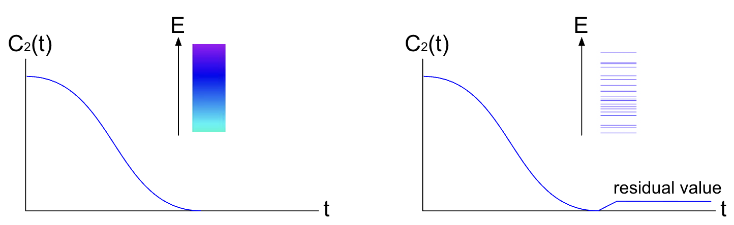
Figure 1: Typical behavior of a two-point function for strongly non-integrable quantum mechanical systems, showing the continuous spectrum (left panel) and discrete spectrum (right panel). The continuous spectrum is associated with type III algebras, which typically arise in the strict thermodynamic limit of many-body quantum systems, where the correlator vanishes. In contrast, the discrete spectrum corresponds to finite-dimensional Hilbert spaces, where the correlator does not vanish. The residual value of the correlator decreases as one increases the number of degrees of freedom.

Quantum Ergodic Hierarchy

Analogous to the classical case, one can define a quantum ergodic hierarchy for quantum systems, which includes:

$$\text{Quantum K-mixing systems}\subset\text{Quantum Mixing systems}\subset\text{Quantum Ergodic systems}.$$

However, it is important to note that the weakest form of chaos in this hierarchy, namely ergodicity, requires the algebra of observables to be of type II, while stronger notions of chaos necessitate an algebra of type III Ouseph:2023juq . In contrast, finite-dimensional quantum systems exhibit an algebra of type I. As a result, there is no quantum chaos in the sense of mixing for finite-dimensional systems. This is why Michael Berry famously stated, “There is no quantum chaos, only quantum chaology” in his well-known paper berry1989quantum . However, under quantization, classically chaotic systems (specifically K-mixing systems) retain memory of their classical chaotic nature, exhibiting correlations in their spectra that resemble those found in random matrix theory BGS . In the thermodynamic limit, the algebra can change from type I to type II or III Witten:2021jzq , allowing the emergence of ergodicity, mixing, and K-mixing. Algebras of type III also arise in quantum field theory and gauge theories at large $N$ Witten:2021jzq . For such systems, with an infinite number of degrees of freedom, one can truly talk about quantum chaos in a way that is parallel to classical chaos because the large-$N$ limit provides a sort of semiclassical limit Richter:2022sik . See Fig. 2 for a comparison with the classical ergodic hierarchy in relation to number of degrees of freedom and “quantumness” of the classical action.

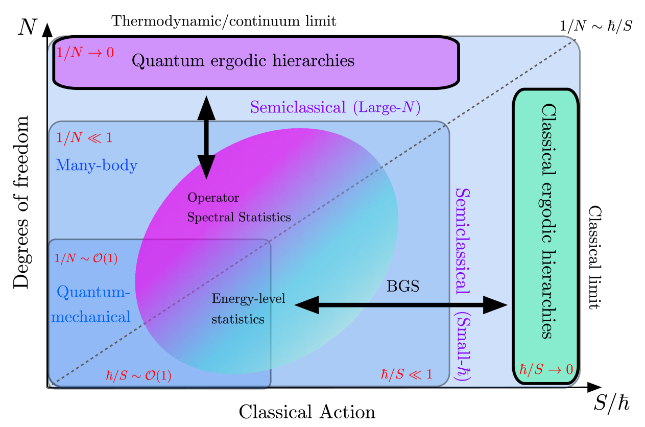
Figure 2: Illustration of the position of the classical and quantum ergodic hierarchies in relation to the number of degrees of freedom $N$, and classical action $S/\hbar$. The classical ergodic hierarchies deal with classical dynamical systems which in the diagram exist in the classical limit $\hbar/S\rightarrow 0$ (right). In contrast, the quantum ergodic hierarchies deal with non-commuting variables and exist only in the strict limit $1/N\rightarrow 0$ (top). As probes of quantum chaos in quantum systems with $1/N>0$, energy-level statistics (arising from the BGS conjecture regarding quantum systems with chaotic classical analogues) and operator spectral statistics do not directly overlap with the quantum ergodic hierarchies. There are different ways in which one can reach an infinite number of degrees of freedom: by considering a lattice model with $L$ sites and taking $L\to\infty$; by taking the continuum limit, where the lattice spacing vanishes, as in QFTs; or by considering a gauge theory matrix/vector model with $N_{c}\to\infty$, where $N_{c}$ is the rank of the gauge group. Note that the parameter $1/N$ plays a role analogous to $\hbar$ in the semi-classical analysis. Diagram inspired by Figure 2 of Richter:2022sik .

The conditions of ergodicity, mixing, and K-mixing all relate to the degree to which operators in the future become statistically independent from those in the past. In the context of free probability theory, there is a concept of statistical independence tailored for non-commutative probability spaces, known as freeness. In subsection 3.1, we introduce this concept and explore its potential application within the quantum ergodic hierarchy.

State Dependence.

The notions of chaos discussed above are defined with respect to a given quantum state, represented by the map $\varphi:\mathcal{A}\to\mathbb{C}$. In this work, we fix the state to be an infinite temperature thermofield double (TFD) state and compute the expectation values of operators $a\in\mathcal{A}$ as $\varphi(a)=\langle\text{TFD}|a|\text{TFD}\rangle$. For operators acting on a single copy of the system, this reduces to a thermal expectation value. This choice is natural, as we aim to work with a state that is well-defined in the thermodynamic limit, and this is always the case for the TFD state Witten:2021jzq . In the case of finite-dimensional systems in which the operators $a_{\mathcal{D}}$ are $\mathcal{D}\times\mathcal{D}$ matrices, we are going to be interested in the expectation value defined as $\varphi(a)=\lim_{\mathcal{D}\rightarrow\infty}\langle\text{TFD}|a_{\mathcal{D}}|\text{TFD}\rangle$.

3.1 Statistical Independence in Quantum Mechanics: Freeness

Given a non-commutative probability space $(\mathcal{A},\varphi)$, two random variables $a,b\in\mathcal{A}$ are said to be free if, for all integers $n\geq 1$ and for all polynomials $P_{1},Q_{1},\dots,P_{n},Q_{n}$ in one variable, we have mingo2017free ; speicher2019lecture

$$\varphi\big{(}(P_{1}(a)-\varphi(P_{1}(a)))(Q_{1}(b)-\varphi(Q_{1}(b)))\cdots(P_{n}(a)-\varphi(P_{n}(a)))(Q_{n}(b)-\varphi(Q_{n}(b)))\big{)}=0\,.$$ (16)

For polynomials of the form $P(x)=Q(x)=x$, and denoting $\varphi(\cdot)=\langle\cdot\rangle$, the above condition implies relations of the form:

$$\langle(a-\langle a\rangle)(b-\langle b\rangle)\rangle=0\,,$$

$$\langle(a-\langle a\rangle)(b-\langle b\rangle)(a-\langle a\rangle)\rangle=0\,,$$

$$\langle(a-\langle a\rangle)(b-\langle b\rangle)(a-\langle a\rangle)(b-\langle b\rangle)\rangle=0\,,$$ (17)

that lead to factorization properties such as

$$\langle ab\rangle=\langle a\rangle\langle b\rangle\,,~~~~\langle aba\rangle=\langle a^{2}\rangle\langle b\rangle\,,~~~~\langle abab\rangle=\langle a^{2}\rangle\langle b\rangle^{2}+\langle a\rangle^{2}\langle b^{2}\rangle-\langle a\rangle^{2}\langle b\rangle^{2}.$$ (18)

Therefore, freeness between $a$ and $b$ can be understood as a notion of independence, as it implies that joint moments involving these variables factorize into products of the individual moments of $a$ and $b$.

Asymptotic Freeness of Large Random Matrices.

Starting from this section, when referring to operators that can be represented as finite dimensional matrices (or finite dimensional random matrices), we use capital letters such as $A$ and $B$, while for general statements about generic random variables we use lower-case letters such as $a$ and $b$.

In the study of large random matrices, it is often useful to consider the behavior of sequences of matrices as their dimension $\mathcal{D}$ approaches infinity. A key concept in this context is the convergence of empirical eigenvalue distributions, which provides a way to analyze the asymptotic spectral properties of these matrices. One important phenomenon that arises in this limit is asymptotic freeness, meaning that certain large random matrices behave as free elements in a non-commutative probability space. For example, independent realizations of Gaussian Unitary Ensemble (GUE) matrices are asymptotically free with respect to the expectation value mingo2017free :

$$\varphi(A)=\lim_{\mathcal{D}\rightarrow\infty}\varphi_{\mathcal{D}}(A)\,,~~~\text{where}~~\varphi_{\mathcal{D}}(A)=\mathbb{E}\left(\frac{{\rm Tr}\,A}{\mathcal{D}}\right),$$ (19)

where $\mathbb{E}$ denotes the ensemble average. Denoting the elements of the operator $A$ as $A_{ij}$, the above map for Gaussian random matrix ensembles is $\varphi(A)=\lim_{\mathcal{D}\rightarrow\infty}\frac{1}{\mathcal{D}}\sum_{i=1}^{\mathcal{D}}\mathbb{E}\left(A_{ii}\right)$.

A fundamental result in this framework states that Haar-distributed unitary conjugation induces asymptotic freeness. Specifically, let $A_{\mathcal{D}}$ and $B_{\mathcal{D}}$ be two sequences of deterministic $\mathcal{D}\times\mathcal{D}$ matrices whose empirical eigenvalue distributions converge as $\mathcal{D}\to\infty$. If $U_{\mathcal{D}}$ is an $\mathcal{D}\times\mathcal{D}$ Haar-distributed unitary random matrix, then:

$$A_{\mathcal{D}},~~\text{and}~~U_{\mathcal{D}}B_{\mathcal{D}}U_{\mathcal{D}}^{\dagger}\quad\text{are asymptotically free as }\mathcal{D}\to\infty,$$ (20)

with respect to the expectation value given in (19). For further details, see mingo2017free .

In the next subsection, we examine how freeness influences the spectral properties of the sum of two free operators.

3.2 Free additive convolution

In this section, we describe how to determine the distribution of the sum of two self-adjoint free random variables. Given two self-adjoint random variables, $a_{1}$ and $a_{2}$, which are free, the distribution of their sum, $a_{1}+a_{2}$, is given by the free convolution of their individual distributions, i.e.,

$$\rho_{a_{1}+a_{2}}=\rho_{a_{1}}\boxplus\rho_{a_{2}}.$$ (21)

This operation, introduced in voiculescu1986addition , provides a non-commutative analogue of classical convolution in probability theory. The procedure for computing $\rho_{a_{1}+a_{2}}$ is outlined below (see speicher2019lecturenotesfreeprobability ; nica2006lectures ; Potters for comprehensive reviews on the subject, and Zee:1996qu ; zinn1999adding for discussions related to random matrices).

For an operator $a$ with eigenvalue density $\rho(\lambda)$ compactly supported on $\mathbb{R}$, the Cauchy transform is defined as

$$G(z)=\int_{\mathbb{I}}\textrm{d}\lambda\,\frac{\rho(\lambda)}{z-\lambda}~,~~~z\in\mathbb{C}\mathbb{I}~,$$ (22)

where $\mathbb{I}$ is the support of the distribution $\rho(\lambda)$ on the real line. For example, for a $\mathcal{D}\times{\mathcal{D}}$ random matrix Hamiltonian ($H$), consider its resolvent defined as, $G_{N}(z)=\frac{1}{{\mathcal{D}}}{\rm Tr}\,\frac{1}{z-H}=\frac{1}{{\mathcal{D}}}\sum_{i}\frac{1}{z-\lambda_{i}}$. Now averaging over the random matrix ensemble, and taking the limit ${\mathcal{D}}\rightarrow\infty$, we have the Cauchy transform of the eigenvalue density: $\mathbb{E}(G_{N}(z))\equiv G(z)=\int_{\mathbb{I}}\textrm{d}\lambda\,\frac{\rho(\lambda)}{z-\lambda}$.

The eigenvalue density $\rho(\lambda)$ can be recovered from the Cauchy transform using the Stieltjes inversion formula:

$$\rho(\lambda)=-\frac{1}{\pi}\lim_{\epsilon\to 0}\left({\rm Im}G(\lambda+i\epsilon)\right).$$ (23)

Since $\rho$ is compactly supported on an interval containing the origin, the inverse of the Cauchy transform, $G^{-1}(z)$, which we denote as $\mathcal{B}(z)$, has a pole at zero and can be decomposed as

$$G^{-1}(z)\equiv\mathcal{B}(z)=\frac{1}{z}+R(z),$$ (24)

where $R(z)$ is called the $R$-transform of $\rho$. The $R$-transform is essentially the regular part of the inverse Cauchy transform after subtracting its singular component. Whereas the Cauchy transform $G(z)$ is analytic in the entire upper half of the complex plane, the $R$-transform is defined for small values of $z$ only and the domain of dependence depends on the eigenvalue density mingo2017free . Since the inverse function $\mathcal{B}(z)$ may have multiple branches, the correct physical solution is determined by requiring that the corresponding $R$-transform satisfies

$$R(0)=0.$$ (25)

This condition ensures the proper analytic continuation and consistency of the transformation.

For two free random variables $a_{1}$ and $a_{2}$ with compactly supported eigenvalue densities $\rho_{a_{1}}$ and $\rho_{a_{2}}$, the $R$-transform of their sum satisfies

$$R_{\rho_{a_{1}}\boxplus\rho_{a_{2}}}(z)=R_{\rho_{a_{1}}}(z)+R_{\rho_{a_{2}}}(z),$$ (26)

for sufficiently small $|z|$ in $\mathbb{C}$. This property provides a method for determining the eigenvalue density of the sum of free operators. Given the $R$-function, the corresponding Cauchy transform $G_{\rho_{a_{1}}\boxplus\rho_{a_{2}}}(z)$ can be computed using equation (24). By applying the Stieltjes inversion formula (23), we obtain the eigenvalue density of the sum:

$$\rho_{a_{1}+a_{2}}(\lambda)=-\frac{1}{\pi}\lim_{\epsilon\to 0}\left({\rm Im}~G_{\rho_{a_{1}}\boxplus\rho_{a_{2}}}(\lambda+i\epsilon)\right).$$ (27)

Since the Cauchy transform, and consequently the eigenvalue density, may admit multiple solutions, the physically relevant solution must be chosen by ensuring positivity within the appropriate domain. There can also be solution for $G_{\rho_{a_{1}}\boxplus\rho_{a_{2}}}(z)$ which are complex conjugates of each other. In that case, one can take the absolute value of any one of these conjugate solutions to get the correct eigenvalue density (see the example of convolution of eigenvalue density of the sum of two free spin-1 operators that we discuss below).

Next, we illustrate the procedure of free additive convolution with two examples.

Example 1. The sum of Spin-1/2 Operators (Bernoulli distribution).

In this case, the eigenvalue density of either of the two operators follows the Bernoulli distribution

$$\rho_{\sigma}(\lambda)=\frac{\delta(\lambda-1)+\delta(\lambda+1)}{2}.$$ (28)

Since both $\rho_{\sigma_{1}}$ and $\rho_{\sigma_{2}}$ have compact supports on $\mathbb{R}$, one can obtain the Cauchy transformation (22) of this distribution to be

$$G_{\rho_{1}}(z)=\frac{z}{z^{2}-1}.$$ (29)

Inverting $G_{\rho_{1}}(z)$, and using the definition in eq. (24) we find the corresponding $R$-transformation is

$$R_{\rho_{1}}(z)=\frac{-1+\sqrt{4z^{2}+1}}{2z}.$$ (30)

Therefore, for two asymptotic free Pauli operators, we have, according to the relation in eq. (26),

$$R_{\rho_{3}}(z)=\frac{\sqrt{1+4z^{2}}-1}{z}.$$ (31)

Next, we obtain $\mathcal{B}_{\rho_{3}}(z)=\frac{1}{z}+R_{\rho_{3}}(z)$, and invert it to find the corresponding Cauchy transformation to be given by

$$G_{\rho_{3}}(z)=\frac{1}{\sqrt{z^{2}-4}}~.$$ (32)

Here, among the two solutions of the quadratic equation for $G_{\rho_{3}}(z)$, we have kept only the one that gives rise to a positive eigenvalue density. After applying eq. (27), we obtain the convolved eigenvalue density of two Pauli operators as

$$\rho_{3}(\lambda)=\rho_{1}(\lambda)\boxplus\rho_{2}(\lambda)=\frac{1}{\pi\sqrt{4-\lambda^{2}}},~~~\text{for}~~|\lambda|<2.$$ (33)

Therefore, the convolved distribution vanishes when $|\lambda|>2$. The distribution in (33) is known as the arcsine distribution in the literature nica2006lectures ; speicher2009free .

Figure 3: Convolved distribution of the sum of two free Pauli operators from free probability theory.

Example 2. The sum of Spin-1 Operators (generalized Bernoulli distribution).

As the next example, we consider the sum of two spin-1 operators $\Sigma$, each of which has three eigenvalues so that the spectrum of individual operators follows a generalized Bernoulli distribution of the form

$$\rho_{\Sigma}(\lambda)=\frac{\delta(\lambda-1)+\delta(\lambda)+\delta(\lambda+1)}{3}.$$ (34)

The Cauchy transform of this distribution can be calculated to be given by

$$G_{\rho_{\Sigma}}(z)=\frac{3z^{2}-1}{3z(z^{2}-1)}.$$ (35)

After finding the inverse function, one can get the R-transformation (here, we discard two other $R$-transformations that do not vanish at $z=0$)

$$\begin{split}R_{\rho_{\Sigma}}(z)=\mathcal{B}_{\rho_{\Sigma}}(z)-\frac{1}{z}=\frac{3z^{2}+(f(z)-1)^{2}}{3zf(z)}~,\\ \text{with}~~f(z)=\Big{(}1+3\sqrt{-z^{2}(1+3z^{2}+3z^{4})}\Big{)}^{1/3}~.\end{split}$$ (36)

The $R$-transform of the eigenvalue density of the sum of two such operators (say, $\Sigma_{1}$ and $\Sigma_{2}$), which are asymptotically free, is the sum of the $R$-transforms of the individual distributions, and hence is given by

$$R_{\rho_{3}}(z)=\frac{6z^{2}+2(f(z)-1)^{2}}{3zf(z)}~.$$ (37)

From this, we first obtain $\mathcal{B}_{\rho_{3}}(z)=R_{\rho_{3}}(z)+\frac{1}{z}$ and calculate the corresponding Cauchy transformation by using the inversion formula $\mathcal{B}_{\rho_{3}}(G_{\rho_{3}}(z))=z$. There are multiple solutions of this equation for the Cauchy transform $G_{\rho_{3}}(z)$. To obtain the correct eigenvalue density, we first plot the function $\mathcal{B}_{\rho_{3}}(G_{\rho_{3}}(z))(=z)$, shown in Fig. 4. There is a region on the vertical axis (from around $-1.92$ to $1.92$) where the function $\mathcal{B}_{\rho_{3}}$ does not attain real values, and hence, this corresponds to the region where the eigenvalues of the sum operator lie. Furthermore, as we have shown in the inset of Fig. 4, this exists between the local minimum and maximum of the function $\mathcal{B}_{\rho_{3}}(G_{\rho_{3}})$. More precisely, we determine the approximate edges of the spectrum of $\Sigma_{3}$ to be between $-1.9227$ to $1.9227$.

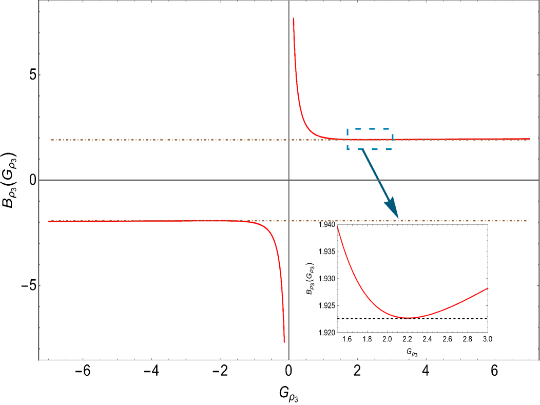
Figure 4: Plot of the function $\mathcal{B}_{\rho_{3}}(G_{\rho_{3}}(z))(=z)$. The edges of the spectrum of $\Sigma_{3}$ are located between a local maximum and minimum of this function. We have shown this minimum more clearly in the inset.

Having determined the range of the spectrum, we now determine the density of eigenvalues of the convoluted operator. As we are eventually looking for a convoluted probability distribution, it should be positive definite in an interval in $\mathbb{R}$, which, in this case, is approximately between $-1.9227$ to $1.9227$.

Since the complex conjugated pair of solutions has the same absolute value of their imaginary parts, from the Stieltjes inverse formula, we can obtain the eigenvalue density of the sum of two spin-1 operators to be

$$\rho_{3}(\lambda)=\lim_{\epsilon\rightarrow 0}\Big{|}\frac{1}{\pi}{\rm Im}~G_{\rho_{3}}(\lambda+i\epsilon)\Big{|}~.$$ (38)

This is plotted in Fig. 5. Furthermore, as one can check, here taking the limit $\epsilon\rightarrow 0$ gives the same distribution as directly substituting $\epsilon=0$, it is possible to obtain the following analytical expression for the distribution shown in Fig. 5 as well,

$$\rho_{3}(\lambda)=\bigg{|}\frac{f_{1}^{2}(\lambda)-4-9\lambda^{4}+33\lambda^{2}}{3\sqrt{3}\pi\lambda\left(\lambda^{2}-4\right)f_{1}(\lambda)}\bigg{|}~,~~~-1.9227\leq\lambda\leq 1.9227~,$$ (39)

where we have defined the function

$$f_{1}(\lambda)=\left(8+9\left(3\lambda^{4}-30\lambda^{2}+70\right)\lambda^{2}+27\sqrt{-\lambda^{2}\left(\lambda^{2}-4\right)^{2}\left(9\lambda^{4}-33\lambda^{2}-1\right)}\right)^{1/3}~.$$ (40)

To the best of our knowledge, the distribution in Equation (39) for the sum of two free spin-1 operators is first derived in this work.

Figure 5: Convolved distribution for the eigenvalue density of the sum of two free spin-1 operators according to free probability theory. The approximate edges of the spectrum, as determined from the plot of the function $\mathcal{B}_{\rho_{3}}(G_{\rho_{3}}(z))(=z)$ in Fig. 4 are, respectively, -1.9227 and 1.9227.

3.2.1 Free additive convolution for arbitrary probability measures

In this section, we briefly review the method described in Section 5 of speicher2019lecturenotesfreeprobability to compute the free additive convolution of arbitrary probability measures. This approach is useful for studying more general algebras, beyond those involving spin-1/2 and spin-1 operators that appear in the models considered in this work.

Consider two free operators, $a$ and $b$, with distributions $\rho_{a}$ and $\rho_{b}$, whose Cauchy transforms are denoted by $G_{a}(z)$ and $G_{b}(z)$, respectively. Their corresponding $R$-transforms are denoted as $R_{a}(z)$ and $R_{b}(z)$. We first define the subordination functions $\omega_{a}(z)$ and $\omega_{b}(z)$ as follows:

$$\omega_{a}(z)=z-R_{b}(G_{\rho_{a}\boxplus\rho_{b}}(z))\,,~~~~\omega_{b}(z)=z-R_{a}(G_{\rho_{a}\boxplus\rho_{b}}(z))\,,$$ (41)

where $G_{\rho_{a}\boxplus\rho_{b}}(z)$ denotes the Cauchy transform of $\rho_{a}\boxplus\rho_{b}$. Then one can show that,

$$G_{\rho_{a}\boxplus\rho_{b}}(z)=G_{a}(\omega_{a}(z))=G_{b}(\omega_{b}(z))\,.$$ (42)

From this the eigenvalue distribution of the sum of these two operators can be obtained via the inverse Stieltjes transform:

$$\rho_{a+b}(\lambda)=-\lim_{\epsilon\rightarrow 0}\frac{1}{\pi}{\rm Im}G_{\rho_{a}\boxplus\rho_{b}}(\lambda+i\epsilon)\,.$$ (43)

Therefore, the problem of determining the distribution $\rho_{a+b}$ can be solved by finding either of the two subordination functions, $\omega_{a}$ or $\omega_{b}$, and then using Eqs. (42) and (43). This can be done numerically as follows. First, one introduces the auxiliary functions:

$$H_{a}(z)=\frac{1}{G_{a}(z)}-z\,,~~~~H_{b}(z)=\frac{1}{G_{b}(z)}-z\,.$$ (44)

These functions satisfy the following fixed-point equation for $\omega_{a}(z)\in\mathbb{C}^{+}$ (the upper half-plane) speicher2019lecturenotesfreeprobability :

$$\omega_{a}(z)=z+H_{b}\left[z+H_{a}(\omega_{a}(z))\right].$$ (45)

For eigenvalue distributions corresponding to the sum of spin-1/2 and spin-1 operators, these equations can be solved analytically. More generally, they can be solved numerically in an iterative manner. For a fixed value of $z$, one starts with an initial guess for $\omega_{a}(z)$ and updates it iteratively using Eq. (45) until convergence. Once $\omega_{a}(z)$ is determined, Eqs. (42) and (43) allow for the numerical computation of $\rho_{a+b}$.

This method only requires knowledge of the Cauchy transform of $a$ and $b$, which is not too difficult to obtain. In Section 3.5, we employ this procedure to compute the free additive convolution for sums of operators with spin-$3/2$, $2$, and $5/2$.

3.3 Asymptotic freeness and the vanishing of OTOCs

Consider a quantum dynamical system $(\mathcal{A},\varphi,T_{t})$, where the time evolution map $T_{t}:\mathcal{A}\to\mathcal{A}$ is given by $A(t)=U^{\dagger}AU$, with the unitary time evolution operator $U=e^{-iHt}$, $H$ being the system’s Hamiltonian. With a focus on many-body quantum systems, we will treat random variables in the algebra as operators represented by matrices of rank $\mathcal{D}$. The quantum state of interest is an infinite temperature TFD state, and the quantum expectation value of a given operator $A\in\mathcal{A}$ is therefore computed as

$$\varphi(A)=\langle\text{TFD}|A|\text{TFD}\rangle\big{|}_{\beta=0}\,.$$ (46)

For an operator acting on a single copy of the system, this is equivalent to an infinite temperature thermal expectation value $\varphi(A)={\rm Tr}\,(A)/\mathcal{D}$. If the model includes random couplings, the expectation value should also account for an average over the couplings, $\varphi(A)=\mathbb{E}\left({\rm Tr}\,(A)/\mathcal{D}\right)$, similar to the procedure in Eq. (19).

Under these conditions, we expect that for two operators $A,B\in\mathcal{A}$, if the dynamics is chaotic, the time-evolved operator $B(t)$ becomes asymptotically free from $A(0)$ with respect to the state (46) at sufficiently large times. This expectation is motivated by the fact that in a chaotic system, the time evolution operator $e^{-iHt}$ is well-approximated by a Haar-random unitary, i.e.,

$$e^{-iHt}\approx U_{\text{Haar}}.$$

From the fundamental result in (20), we know that two deterministic matrices $A$ and $B$ are expected to be free when one of them is conjugated by a Haar-random unitary. That is, for two matrices $A$ and $B$ of rank $\mathcal{D}$, when $U$ is a Haar-random unitary matrix of size $\mathcal{D}\times\mathcal{D}$, the conjugated matrix $U_{\text{Haar}}^{\dagger}BU_{\text{Haar}}$ becomes asymptotically free from $A$ with respect to the state $\varphi(A)=\mathbb{E}\left({\rm Tr}\,(A)/\mathcal{D}\right)$ in the limit $\mathcal{D}\to\infty$.

The asymptotic freeness between $A(0)$ and $B(t)$ implies that all mixed cumulants involving these operators vanish in the limit $\mathcal{D}\to\infty$. In particular, if we consider operators with zero expectation values, $\langle A\rangle=0$ and $\langle B(t)\rangle=0$, this leads to the vanishing of the following cumulants:

$$\langle A(0)B(t)\rangle\,,~~~\langle A(0)B(t)A(0)B(t)\rangle\,,~~~\langle A(0)B(t)A(0)B(t)A(0)B(t)\rangle$$

for sufficiently large times, as well as cumulants involving an odd number of operators. The vanishing of the two-point function $\langle A(0)B(t)\rangle$ is associated with thermalization, while the vanishing of the four-point OTOC $\langle A(0)B(t)A(0)B(t)\rangle$, as well as its higher-order counterparts, is linked to the scrambling of quantum information.

The asymptotic freeness between two operators $A$ and $B(t)$ can alternatively be understood as arising from the fact that, for sufficiently large times, these operators not only fail to commute but also exhibit a large commutator. Notably, this captures the same effect as the squared commutator, $C(t)=-\langle[A,B(t)]^{2}\rangle$, thereby making the connection with scrambling and operator growth particularly transparent. However, asymptotic freeness is an even stronger condition, as it implies not only that the squared commutator is large but also that all its higher-order generalizations, $C_{(k)}(t)=-\langle[A,B(t)]^{2k}\rangle$, are large as well.

3.4 Incorporating Freeness into the Quantum Ergodic Hierarchy

The previous discussions motivate the inclusion of freeness into the quantum ergodic hierarchy. We propose the following definition:

F-systems.

A quantum dynamical system $(\mathcal{A},\varphi,T_{t})$ is said to be an F-system or to possess the F-property if, for any operators $A,B\in\mathcal{A}$, the operators $A$ and $B(t)$ are free in the limit $t\to\infty$. We also refer to the F-property as freeness.

It is clear that the F-property implies quantum mixing, but it is unclear whether this condition is stronger or weaker than quantum $K$-mixing. We suspect that the F-property, or freeness, lies between quantum mixing and quantum $K$-mixing in the ergodic hierarchy. See Figure 6.

3.5 Operator statistics as a signature of asymptotic freeness

The fact that freeness can only emerge in the large $\mathcal{D}$ limit can be understood from an algebraic perspective, particularly in the context of the quantum ergodic hierarchy. First, observe that freeness implies 2-mixing. Since mixing is a property that arises only for type III algebras, it follows that freeness can occur only for type III algebras. For finite $\mathcal{D}$, however, the algebra of observables is always of type I, and therefore freeness cannot occur. As a result, mixed free cumulants of centered variables ($A-\langle A\rangle$ and $B(t)-\langle B(t)\rangle$) will not generically vanish for finite $\mathcal{D}$. However, if the dynamics is chaotic, these cumulants are expected to approach a small residual value that scales inversely with the number of degrees of freedom in the system. This expectation was indeed shown to be true for OTOCs in Huang:2017fng . Furthermore, if two operators $A$ and $B(t)$ are free, the eigenvalue density of their sum $\rho_{A(0)+B(t)}$ is expected to follow the free convolution prediction, which can emerge even for finite, but sufficiently large $\mathcal{D}$, and serves as a “smoking gun” of asymptotic freeness Chen:2024zfj . These concepts are illustrated schematically in Figure 6.

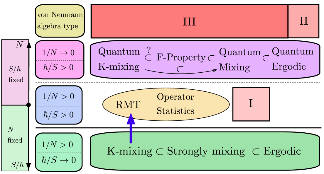
Figure 6: Illustration of the quantum and classical ergodic hierarchies, with freeness (F-property) positioned between quantum mixing and K-mixing. This placement is not fully established and remains an open question, as the precise relationship between these concepts is still under investigation. $N$ denotes the number of degrees of freedom of the system. The corresponding von Neumann algebraic structures associated with different degrees of quantum chaos are indicated. Note that the quantum hierarchy is only meaningful in the $1/N\rightarrow 0$ limit, as for any finite $N$, the algebra remains type I, preventing even ergodicity. Nonetheless, a finite-$N$ system can exhibit signatures of its asymptotic behavior. For example, the emergence of operator spectral statistics governed by free probability theory serves as a robust indicator of asymptotic freeness.

We illustrate this idea by studying the spectrum of operators of the form

$$X^{(s)}_{i}+U^{\dagger}X^{(s)}_{i}U$$ (47)

where the time evolution operator is $U=e^{-it\,M}$, with $M$ being a random matrix drawn from a Gaussian orthogonal ensemble (GOE), and $X^{(s)}_{i}$ are generalized spin-$s$ operators (see Sec. 5 for a precise definition). For a chain with $L$ sites, these operators have dimension $d_{s}=(2s+1)^{L}$. The variance of $M$ was fixed at $2/d_{s}$. Figure 7 shows the spectrum of $X^{(s)}_{i}+U^{\dagger}X^{(s)}_{i}U$ for spin-$1/2$ operators (left panel) and spin-1 operators (right panel), along with the free convolution prediction for the corresponding operators (see eqs. (33) and (39)). Figure 8 shows the spectrum of $X^{(s)}_{i}+U^{\dagger}X^{(s)}_{i}U$ for spin-$3/2$, spin-2, and spin-$5/2$ operators, along with the numerical free convolution prediction for the corresponding operators, obtained using the method described in Section 3.2.1. These results demonstrate that when the dynamics are driven by a random matrix, the spectrum of $X^{(s)}_{i}+U^{\dagger}X^{(s)}_{i}U$ aligns with the predictions of free probability. This is expected in light of (20).

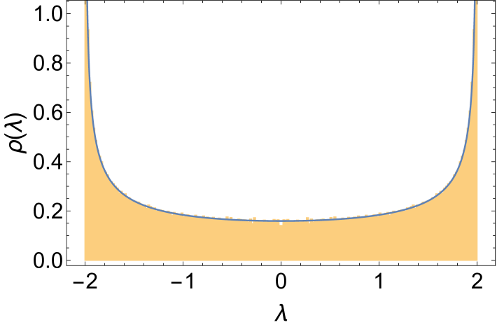
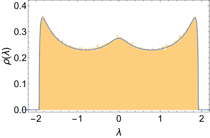
Figure 7: Density of eigenvalues for the operator sum $X^{(s)}_{i}+U^{\dagger}X^{(s)}_{i}U$, where $X^{(s)}$ spin-$s$ operators and $U=e^{-itM}$ represents the time evolution operator. Here we set $t=50$. The matrix $M$ is drawn from a GOE with zero mean and variance $2/d_{s}$, where $d_{s}=(2s+1)^{L}$ is the Hilbert space dimension for a spin-$s$ chain with $L$ sites. The histograms are based on 100 independent realizations of $M$. The left panel corresponds to spin-$1/2$ operators with $(s,L)=(1/2,10)$, while the right panel shows results for spin-1 operators with $(s,L)=(1,6)$. The blue curves represent the free probability prediction.

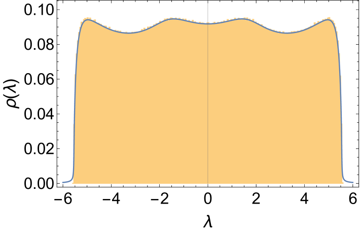
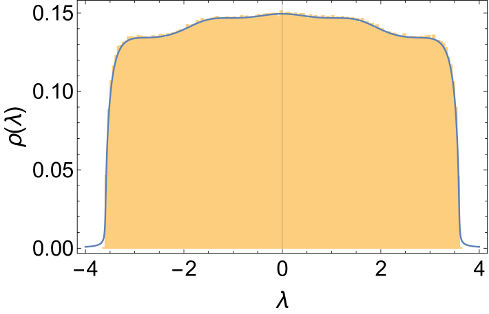
(a) spin-3/2	(b) spin-2
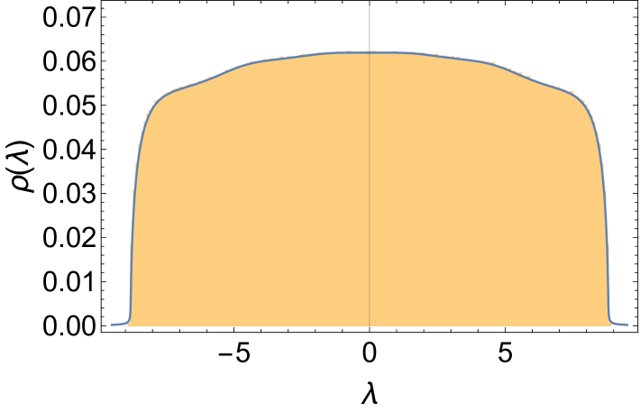
(c) spin-5/2

Figure 8: Density of eigenvalues for the operator sum $X^{(s)}_{i}+U^{\dagger}X^{(s)}_{i}U$, where $X^{(s)}$ spin-$s$ operators and $U=e^{-itM}$ represents the time evolution operator. Here we set $t=50$. The matrix $M$ is drawn from a GOE with zero mean and variance $2/d_{s}$, where $d_{s}=(2s+1)^{L}$ is the Hilbert space dimension for a spin-$s$ chain with $L$ sites. The histograms are based on 1000 independent realizations of $M$. Panels correspond to (a) spin-3/2 operators with $L=5$, (b) spin-2 operators with $L=4$, and (c) spin-5/2 operators with $L=4$. The operators are normalized such that their distribution reads $\rho_{s=3/2}=\frac{1}{4}(\delta_{-3}+\delta_{-1}+\delta_{1}+\delta_{3})$, $\rho_{s=2}=\frac{1}{5}(\delta_{-2}+\delta_{-1}+\delta_{0}+\delta_{1}+\delta_{2})$, and $\rho_{s=5/2}=\frac{1}{6}(\delta_{-5}+\delta_{-3}+\delta_{-1}+\delta_{1}+\delta_{3}+\delta_{5})$. The blue curves represent the free probability prediction obtained using the method described in Section 3.2.1.

Next three sections describe how one can use the free additive convolution prediction to probe chaos in quantum many-body systems.

4 Asymptotic Freeness in the Mixed-Field Ising Model

As the first example of studying the emergence of asymptotic freeness in realistic many-body quantum systems, we consider the one-dimensional mixed-field Ising model with open boundary conditions:

$$H_{0}=-\sum_{i=1}^{L-1}Z_{i}Z_{i+1}-\sum_{i=1}^{L}\left(h_{x}X_{i}+h_{z}Z_{i}\right)\,,$$ (48)

where $X_{i},Y_{i},$ and $Z_{i}$ are Pauli matrices acting on the $i$th site. For example:

$$X_{i}=\left(\mathds{1}_{2}\right)^{\otimes(i-1)}\otimes\sigma_{x}\otimes\left(\mathds{1}_{2}\right)^{\otimes(L-i)}~,$$ (49)

with similar formulas for $Y_{i}$ and $Z_{i}$. For a fixed number of sites $L$, the dimension of the Hilbert space is $d=2^{L}$.

The model (48) is integrable if either $h_{x}=0$ or $h_{z}=0$, and it is non-integrable if both parameters are finite and nonzero. In particular, for $(h_{x},h_{z})=(-1.05,0.5)$, this model displays nearest-neighbor level spacing statistics well-described by random matrix theory associated with chaotic dynamics. See for instance Ba_uls_2011 ; Craps:2019rbj .

For any values of $(h_{x},h_{z})$, this model has parity symmetry – the Hamiltonian (48) commutes with the parity operator

$$\hat{\Pi}=\begin{cases}\hat{P}_{1,L}\,\hat{P}_{2,L-1}\,\cdots\,\hat{P}_{\frac{L}{2},\frac{L+2}{2}}\,,\,\,\quad\text{for}\,\,L\,\,\text{even}\\ \hat{P}_{1,L}\,\hat{P}_{2,L-1}\,\cdots\,\hat{P}_{\frac{L-1}{2},\frac{L+3}{2}}\,,\,\,\,\text{for}\,\,L\,\,\text{odd}\end{cases}$$ (50)

where the permutation operator

$$\hat{P}_{i,j}=\frac{1}{2}\left(\mathds{1}_{d}+X_{i}X_{j}+Y_{i}Y_{j}+Z_{i}Z_{j}\right)$$ (51)

permutes the spin configuration of the sites $i^{\text{th}}$ and $j^{\text{th}}$. The action of the parity operator on a given state can be understood by imagining a mirror at one edge of the chain. The action of $\hat{\Pi}$ on a given spin configuration (state) returns the mirror image of that spin configuration.

Model with a random magnetic field.

We also study a variant of the Ising model where parity symmetry is broken by introducing a random magnetic field:

$$H_{d}=\sum_{i=1}^{L}\epsilon_{i}X_{i}\,,$$ (52)

where $\epsilon_{i}$ is drawn from a Gaussian distribution with average zero and unit variance. In this case, the full Hamiltonian takes the form

$$H=H_{0}+gH_{d}\,.$$ (53)

This modified model is particularly advantageous for spectral statistics analysis for two reasons. First, the absence of parity symmetry simplifies the level-spacing statistics analysis, as there is no need to decompose the Hamiltonian into block diagonal form. Second, by analyzing multiple realizations of the random magnetic field in Eq. (52), it is possible to gather a large number of eigenvalues (on the order of half a million) without significantly increasing the system size. This approach allows for efficient computations while maintaining statistical reliability.

4.1 Spectral statistics of the Hamiltonian

The nearest-neighbor level spacing statistics of the Hamiltonian (53) is shown in Fig. 9. After fixing $g=0.2$, the level spacing statistics is well described by a Poisson distribution for $(h_{x},h_{z})=(-1,0)$, which transitions to a GOE-type Wigner-Dyson distribution for $(h_{x},h_{z})=(-1.05,0.5)$.

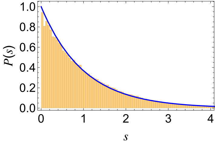
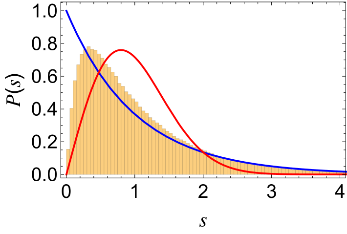
(a)	(b)
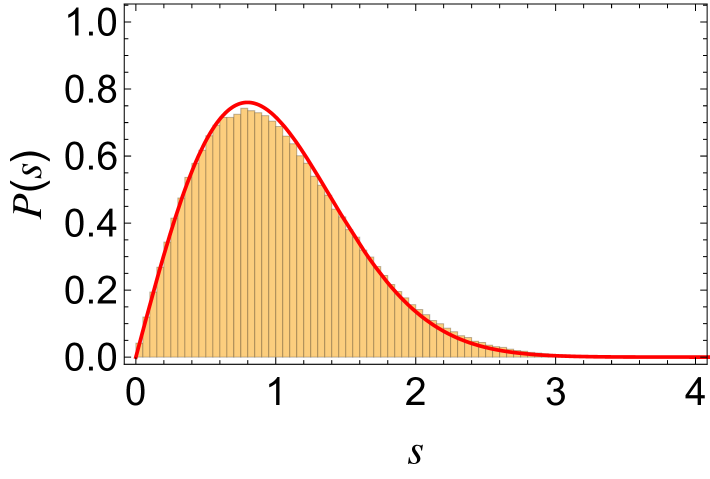
(c)

Figure 9: Spectral statistics for 1000 realizations of the Hamiltonian (53) with $L=10$ and $g=0.2$. Panels correspond to: (a) the near-integrable regime at $(h_{x},h_{z})=(-1,0)$, (b) the intermediate regime at $(h_{x},h_{z})=(-1.05,0.03)$, and (c) the chaotic regime at $(h_{x},h_{z})=(-1.05,0.5)$. The values of the corresponding average $r$-parameter are $0.38$, $0.45$, and $0.53$, respectively. The blue line represents the Poisson distribution, while the red line corresponds to the Wigner-Dyson distribution for $\nu=1$ (GOE). The analysis focuses on the central 50% of the spectrum, excluding the outermost 25% on each edge.

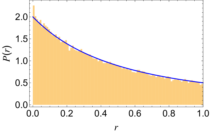
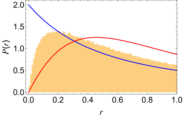
(a)	(b)
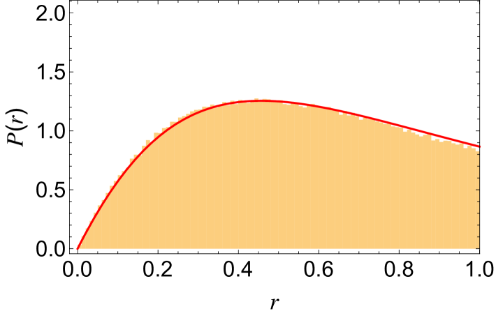
(c)

Figure 10: $r$-parameter statistics for 1000 realizations of the Hamiltonian (53) with $L=10$ and $g=0.2$. Panels correspond to: (a) the near-integrable regime at $(h_{x},h_{z})=(-1,0)$, (b) the intermediate regime at $(h_{x},h_{z})=(-1.05,0.03)$, and (c) the chaotic regime at $(h_{x},h_{z})=(-1.05,0.5)$. The values of the corresponding average $r$-parameter are $0.38$, $0.45$, and $0.53$, respectively. The blue line represents the Poisson $r$-parameter distribution, while the red line corresponds to the Wigner-Dyson $r$-parameter distribution for $\nu=1$ (GOE). The analysis focuses on the central 50% of the spectrum, excluding the outermost 25% on each edge.

In spin chains, such as the Hamiltonian (53), the density of states typically follows a Gaussian distribution, which simplifies the unfolding of the spectrum. However, for more general Hamiltonians, like the mass-deformed SYK model, the density of states transitions from a Wigner semicircle distribution to a deformed Gaussian as one moves from the chaotic to the integrable regime. This transition complicates both the determination of the average density of states and the unfolding procedure. To bypass these complications, it is convenient to instead focus on the $r$-parameter statistics, which do not require any unfolding. A brief review of the $r$-parameter statistics is provided in Appendix C. Figure 10 displays the $r$-parameter statistics for the Hamiltonian (53) at the chaotic, intermediate, and near-integrable points. The degree of chaoticity, in terms of random matrix behavior, can be evaluated using the average $r$-parameter. This parameter takes a value of 0.38 for uncorrelated spectra, typical of integrable systems, and 0.53 for spectra that exhibit GOE-type random matrix statistics. In Figure 11, we show how the average $r$-parameter evolves from 0.38 to 0.53 as a function of the coupling $h_{z}$.

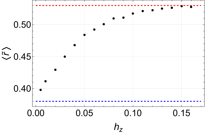
Figure 11: Average $r$-parameter versus $h_{z}$ for 1000 realizations of the Hamiltonian (53) with $h_{x}=-1$, $g=0.2$, and $L=10$. The dashed blue and red lines indicate the average $r$-parameter for spectra whose level spacing distributions follow Poisson and GOE-type Wigner-Dyson statistics, respectively, with values of approximately 0.38 and 0.53. The analysis focuses on the central 50% of the spectrum, excluding the outermost 25% on each edge.

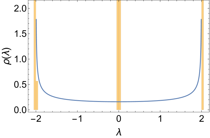
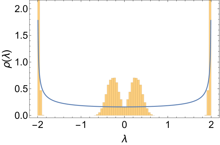
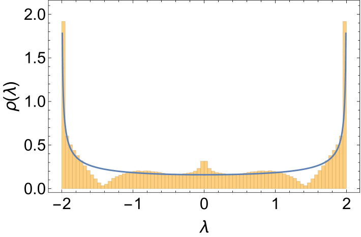
Figure 12: Spectrum of eigenvalues the operator $Z_{1}(0)+Z_{10}(t)$ for increasing values of time at the chaotic point. Here we fix $(h_{x},h_{z},g)=(-1.05,0.5,0.2)$, and $L=10$ and consider 100 realizations of the Hamiltonian (53). The number of bins in each histogram is $100$.

4.2 Approximate emergence of asymptotic freeness

In this section, we examine the spectral statistics of operators of the form $Z_{i}(0)+Z_{j}(t)$, where the generalized Pauli operator is time-evolved under the Hamiltonian (53). Both $Z_{i}(0)$ and $Z_{j}(t)$ have eigenvalues $\pm 1$, characterized by a Bernoulli distribution. When these operators are asymptotically free, the spectrum of their sum is expected to follow an arcsine distribution (see Example 1 in section 3.2):

$$f(\lambda)=\begin{cases}\frac{1}{\pi\sqrt{4-\lambda^{2}}},&\text{if }0<\lambda<1,\\ 0,&\text{otherwise.}\end{cases}$$ (54)

Asymptotic freeness is anticipated in chaotic dynamics but not in integrable dynamics. Figure 12 illustrates the spectrum of $Z_{1}(0)+Z_{10}(t)$ at the chaotic point of the Hamiltonian (53), while Figure 13 shows the same for a near-integrable point. The arcsine law manifests as long as the dynamics are non-integrable; however, the timescale at which it emerges grows rapidly as the system approaches the integrable limit. In fully integrable dynamics, the arcsine law does not emerge. In the following, we introduce a methodology to determine the time scale at which the arcsine law emerges.

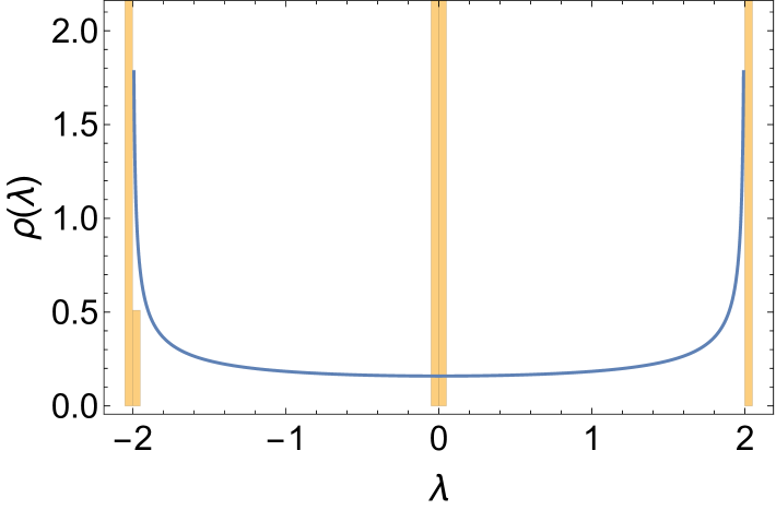
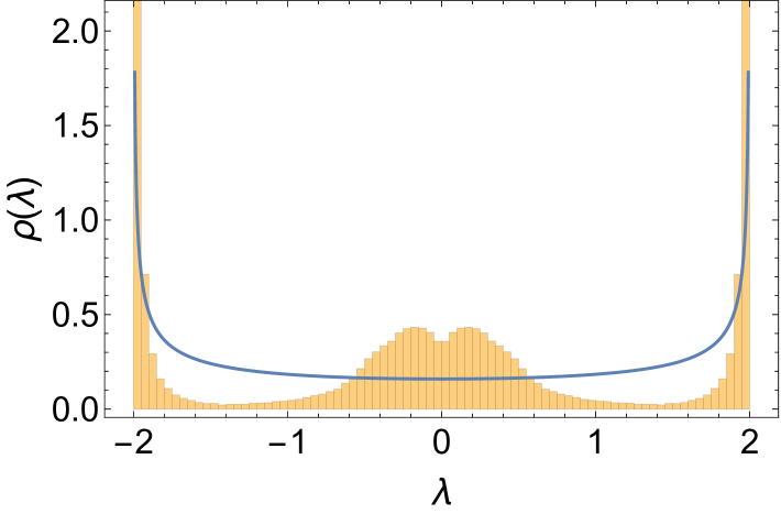
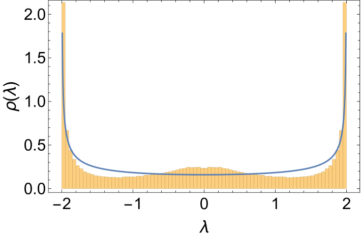
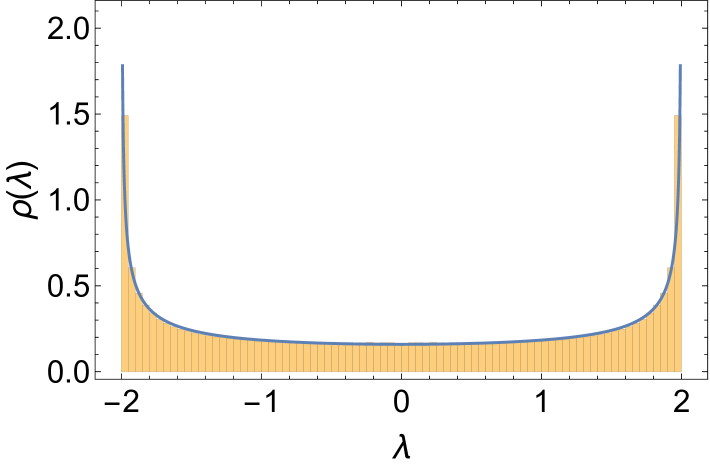
Figure 13: Spectrum of eigenvalues of the operator $Z_{1}(0)+Z_{10}(t)$ for increasing time at the near-integrable point. The parameters are set to $(h_{x},h_{z},g)=(-1,0.005,0.2)$ and $L=10$, with 100 realizations of the Hamiltonian (53). The number of bins in each histogram is $100$.

Methodology to determine the arcsine time.

To identify the time at which the arcsine law emerges, we employ a least-squares procedure. Specifically, we compute the following quantity, which quantifies the deviation of the eigenvalue distribution from the arcsine law:

$$\chi^{2}=\sum_{i}\left(\frac{\rho(\lambda_{i})-f(\lambda_{i})}{f(\lambda_{i})}\right)^{2}\,,$$ (55)

where $\rho(\lambda_{i};t)$ represents the density of eigenvalues obtained from the histogram of eigenvalues of $A(0)+B(t)$ at time $t$, and $f(\lambda_{i})$ is defined in Eq. (54).

The arcsine time scale is estimated as follows: at early times, $\rho(\lambda_{i};t)$ deviates significantly from the arcsine distribution, resulting in large values of $\chi^{2}$. As the time parameter $t$ increases, $\chi^{2}$ decreases until it reaches an approximately constant value, around which it oscillates. To determine the time scale at which $\chi^{2}$ stabilizes, we fit a function of the form

$$F(t)=A\,e^{-(t-t_{0})/t_{d}}+A\,,$$ (56)

to the $\chi^{2}$ data points, starting from the time scale near saturation up to later times where the data oscillates around a constant value. From this fit, we extract the parameters $A$, $t_{0}$, and $t_{d}$, and define the arcsine time as $t_{\text{arcsine}}=t_{0}+t_{d}$. It is important to note that this time scale does not exactly correspond to the point where $\chi^{2}$ becomes constant, since $F(t_{\text{arcsine}})=A/e+A$. Instead, it marks the time scale at which the arcsine law emerges. See Figure 14. Alternatively, one could define the time scale $t^{(n)}_{\text{arcsine}}=t_{0}+n\,t_{d}$, with $n=2,3,\dots$, at which $F(t_{\text{arcsine}})=A/e^{n}+A$. This alternative definition yields qualitatively similar results. Figure 15 illustrates how the arcsine time depends on the average $r$-parameter.

One important limitation of the above analysis is that it is based on a single realization of the Hamiltonian (53). This choice was made to enable the study of the spectral properties of operators as a function of time and to perform a least-squares analysis within a reasonable computational time. Specifically, we consider a single realization of the Hamiltonian (53) with $L=10$, resulting in an analysis based on only 1024 eigenvalues, which introduces substantial statistical uncertainties. Nevertheless, the analysis effectively illustrates how the arcsine time depends on the degree of chaoticity of the system and diverges as one approaches integrability. In a later section, a more refined analysis, based on 1000 realizations of the Hamiltonian (53), reveals small deviations from the arcsine law, particularly for the $X$-Pauli operators.

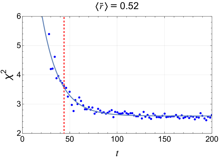
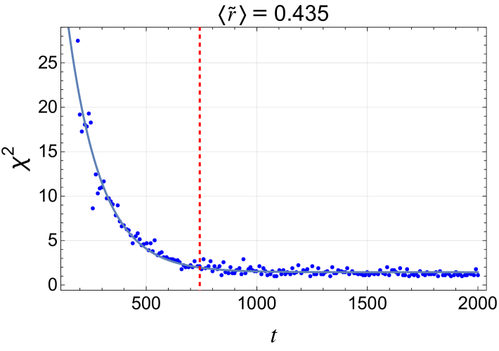
Figure 14: Time evolution of $\chi^{2}$ for the operator $Z_{1}(0)+Z_{10}(t)$ for two distinct average $r$-parameter values: $\langle\tilde{r}\rangle=0.52$ (left panel) and $\langle\tilde{r}\rangle=0.435$ (right panel). Both panels share fixed parameters $g=2$, $L=10$, and $h_{x}=-1$, while $h_{z}$ differs between the panels: $h_{z}=0.1$ (left) and $h_{z}=0.023$ (right). The fitted function, $F(t)=Ae^{-(t-t_{0})/t_{d}}+A$, is shown as a continuous line, where $A$, $t_{0}$, and $t_{d}$ are fitting parameters. The arcsine times, estimated as $t_{\text{arcsine}}=t_{0}+t_{d}$, are $t_{\text{arcsine}}=44\pm 1$ (left) and $t_{\text{arcsine}}=742\pm 17$ (right) and are marked by vertical dashed red lines. The analysis is based on a single realization of the Hamiltonian (53).

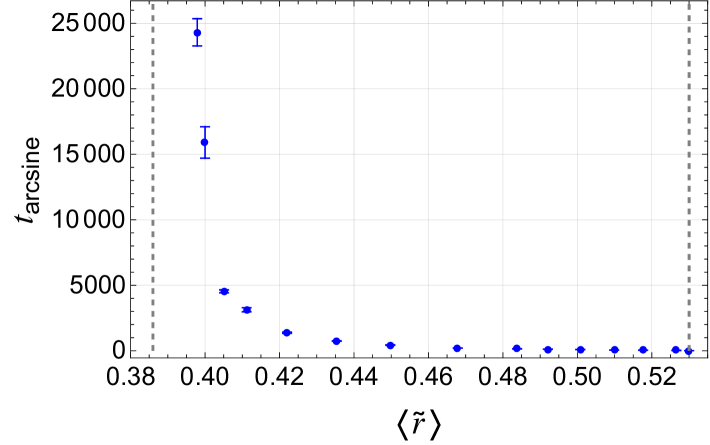
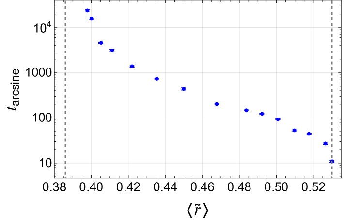
Figure 15: Time scale for the emergence of the arcsine law for the operator $Z_{1}(0)+Z_{10}(t)$ as a function of the average $r$-parameter, $\langle\tilde{r}\rangle$. The left/right panel shows the results in a linear/logarithmic scale. The parameters are fixed at $g=0.2$ and $L=10$, while $h_{x}$ and $h_{z}$ are varied to span $\langle\tilde{r}\rangle$ from 0.53 (indicating GOE statistics) to approximately 0.38 (indicating Poisson statistics). Vertical gray dashed lines mark these characteristic values of $\langle\tilde{r}\rangle$. The analysis is based on a single realization of the Hamiltonian (53).

4.3 Fluctuations on top of the arcsine law

In random matrix theory, the average density of states follows the Wigner semicircle law, with fluctuations exhibiting universal properties described by the Wigner-Dyson distribution of the appropriate universality class. Since the arcsine law governs the average density of states for operators of the form $A(0)+B(t)$ in non-integrable systems, it is natural to investigate whether the fluctuations on top of it also exhibit universal properties. A precise spectral statistics analysis requires a sufficiently large number of eigenvalues. To achieve this, the analysis below was performed using 1000 realizations of the Hamiltonian (53), yielding a total of 1,024,000 eigenvalues. The level spacing and $r$-parameter statistics were computed using the central 50% of the spectrum, resulting in approximately half a million eigenvalues.

Fluctuations at the chaotic point.

Figure 16 presents the eigenvalue density, the level spacing distribution, and the $r$-parameter distribution for the operator $X_{1}+X_{10}(t)$, based on 1000 realizations of the Hamiltonian (53) at the chaotic point $(h_{x},h_{z},g)=(-1.05,0.5,0.2)$, with $L=10$ and $t=50$. In panel (a), the improved statistics reveal deviations from the arcsine law, particularly near the edges of the spectrum, indicating that the arcsine law emerges only in an approximate sense. In panel (b), the level spacing statistics of the operator closely resemble the Wigner-Dyson distribution with Dyson index $\nu=2$, corresponding to the GUE of random matrices. However, some deviations are observed, possibly due to imperfect unfolding of the spectrum, which was performed using the arcsine law as the average density of eigenvalues. Panel (c) shows that the $r$-parameter distribution is well described by the Wigner $r$-parameter distribution with $\nu=2$, yielding an average value of $\langle\tilde{r}\rangle=0.60$. Figure 17 presents similar results for the operator $Z_{1}+Z_{10}(t)$, with the key difference that the arcsine law and the Wigner-Dyson level spacing distribution fit the data very well in this case.

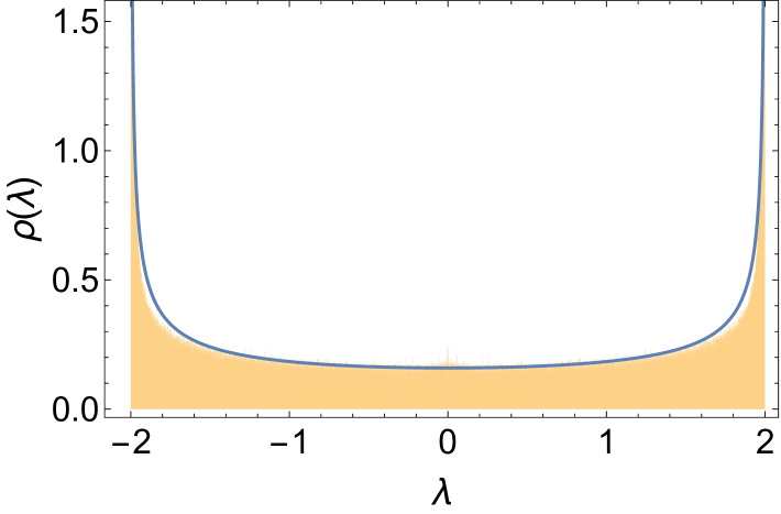
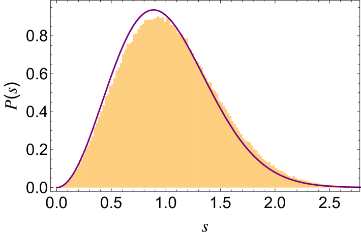
(a) Eigenvalue density	(b) Level spacing distribution
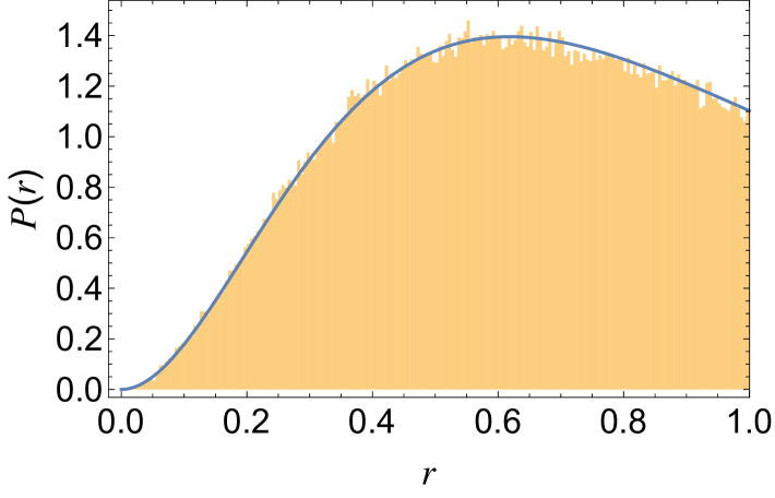
(c) $r$-parameter distribution

Figure 16: Eigenvalue density, level spacing distribution, and $r$-parameter distribution for the operator $X_{1}+X_{10}(t)$ based on 1000 realizations of the Hamiltonian (53) at the chaotic point $(h_{x},h_{z},g)=(-1.05,0.5,0.2)$, with $L=10$ and $t=50$. The $r$-parameter distribution was fitted using the form (83), yielding the Wigner parameter $\nu=2.000\pm 0.002$. The solid lines represent (a) the arcsine distribution, (b) the Wigner-Dyson distribution with $\nu=2$, and (c) the Wigner $r$-parameter distribution with $\nu=2$. The corresponding average $r$-parameter was found to be $\langle\tilde{r}\rangle=0.60$. The analysis focuses on the central 50% of the spectrum, excluding the outermost 25% at each edge.

Fluctuations at the near-integrable point.

Figure 18 presents the eigenvalue density, the level spacing distribution, and the $r$-parameter distribution for the operator $X_{1}+X_{10}(t)$, based on 1000 realizations of the Hamiltonian (53) at the near-integrable point $(h_{x},h_{z},g)=(-1.0,0.005,0.2)$, with $L=10$ and $t=5\times 10^{4}$. In panel (a), the improved statistics reveal deviations from the arcsine law even at very large times, which are substantially larger compared to the chaotic case, indicating that the arcsine law has not emerged at this time scale, highlighting limitations in analyzing the emergence of the arcsine law based on a single realization of the Hamiltonian (53). As can be seen from panel (b), the level spacing statistics of the operator exhibit level spacing repulsion and resemble the Wigner-Dyson distribution with $\nu=2$, though with larger deviations compared to the chaotic case, possibly due to imperfect unfolding of the spectrum, which was performed using the arcsine law as the average density of eigenvalues. Panel (c) shows that the $r$-parameter distribution is well described by the Wigner $r$-parameter distribution with $\nu=2$, yielding an average value of $\langle\tilde{r}\rangle=0.60$. Figure 19 presents similar results for the operator $Z_{1}+Z_{10}(t)$, with the key difference that the arcsine law and the Wigner-Dyson level spacing distribution fit the data very well in this case.

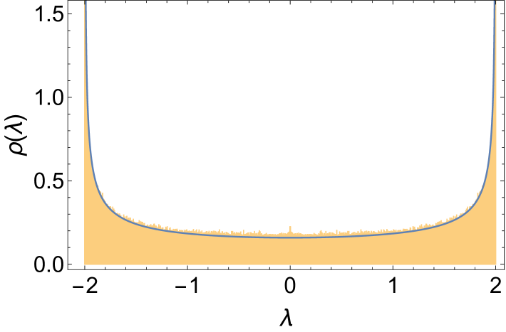
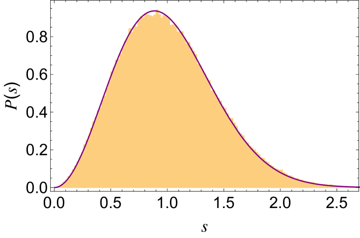
(a) Eigenvalue density	(b) Level spacing distribution
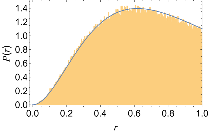
(c) $r$-parameter distribution

Figure 17: Eigenvalue density, level spacing distribution, and $r$-parameter distribution for the operator $Z_{1}+Z_{10}(t)$ based on 1000 realizations of the Hamiltonian (53) at the chaotic point $(h_{x},h_{z},g)=(-1.05,0.5,0.2)$, with $L=10$ and $t=50$. The $r$-parameter distribution was fitted using the form (83), yielding the Wigner parameter $\nu=2.000\pm 0.002$. The solid lines represent (a) the arcsine distribution, (b) the Wigner-Dyson distribution with $\nu=2$, and (c) the Wigner $r$-parameter distribution with $\nu=2$. The corresponding average $r$-parameter was found to be $\langle\tilde{r}\rangle=0.60$. The analysis focuses on the central 50% of the spectrum, excluding the outermost 25% at each edge.

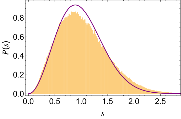
(a) Eigenvalue density	(b) Level spacing distribution
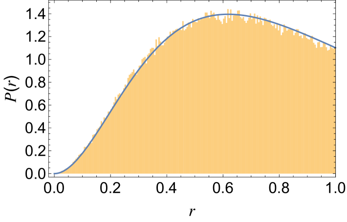
(c) $r$-parameter distribution

Figure 18: Eigenvalue density, level spacing distribution, and $r$-parameter distribution for the operator $X_{1}+X_{10}(t)$ based on 1000 realizations of the Hamiltonian (53) at the near-integrable point $(h_{x},h_{z},g)=(-1,0.005,0.2)$, with $L=10$ and $t=5\times 10^{4}$. The $r$-parameter distribution was fitted using the form (83), yielding the Wigner parameter $\nu=2.001\pm 0.002$. The solid lines represent (a) the arcsine distribution, (b) the Wigner-Dyson distribution with $\nu=2$, and (c) the Wigner $r$-parameter distribution with $\nu=2$. The corresponding average $r$-parameter was found to be $\langle\tilde{r}\rangle=0.60$. The analysis focuses on the central 50% of the spectrum, excluding the outermost 25% at each edge.

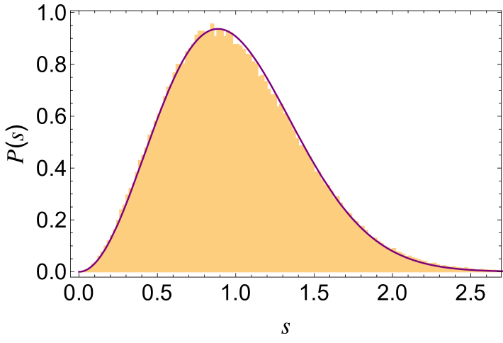
(a) Eigenvalue density	(b) Level spacing distribution
(c) $r$-parameter distribution

Figure 19: Eigenvalue density, level spacing distribution, and $r$-parameter distribution for the operator $Z_{1}+Z_{10}(t)$ based on 1000 realizations of the Hamiltonian (53) at the near-integrable point $(h_{x},h_{z},g)=(-1,0.005,0.2)$, with $L=10$ and $t=5\times 10^{4}$. The $r$-parameter distribution was fitted using the form (83), yielding the Wigner parameter $\nu=2.001\pm 0.002$. The solid lines represent (a) the arcsine distribution, (b) the Wigner-Dyson distribution with $\nu=2$, and (c) the Wigner $r$-parameter distribution with $\nu=2$. The corresponding average $r$-parameter was found to be $\langle\tilde{r}\rangle=0.60$. The analysis focuses on the central 50% of the spectrum, excluding the outermost 25% at each edge.

The primary takeaway from the above numerical analysis is that the free probability prediction for the spectrum of the operator $X_{1}+X_{10}(t)$ – specifically, the arcsine law – emerges only approximately within the time scales considered for a single realization of the Hamiltonian (53). Despite this approximate emergence, the arcsine law appears even near the integrable point, with fluctuations exhibiting random matrix behavior. This is particularly evident in the $r$-parameter statistics. The observed deviations in the level spacing statistics are likely due to imperfections in the unfolding process of the spectrum. Both the chaotic and near-integrable points exhibit universal level spacing statistics for the eigenvalues $X_{1}+X_{10}(t)$ with the key distinction being that, in the near-integrable case, this behavior emerges only at much later times. By contrast, for the operator $Z_{1}+Z_{10}(t)$, the arcsine law fits the data well even in the near-integrable point, and the fluctuations are well described by a Wigner-Dyson distribution.

In finite numerical simulations, free cumulants in the model (53) do not vanish due to finite-size effects. The above results show that while the dynamics drives $Z_{1}$ and $Z_{10}(t)$ towards asymptotic freeness – producing a spectrum for their sum that respects the free probability prediction – the same is not entirely true for $X$-Pauli operators, in which one observes small deviations from the free probability prediction even at the chaotic point. This suggests that the finite size effects for mixed cumulants involving $X$-Pauli operators are larger than the ones involving $Z$-Pauli operator, which is indeed what is observed in numerical simulations.

5 Asymptotic Freeness in the High-Spin Mixed-Field Ising Model

In this section, we consider a spin-$s$ generalization of the mixed-field Ising model (52), where the spin-$\frac{1}{2}$ particles at each site are replaced by spin-$s$ representations of $SU(2)$, and study the emergence of asymptotic freeness of operators under time evolution generated by this Hamiltonian. We start with the model proposed in Craps:2019rbj :

$$H^{(s)}=-2\frac{\sqrt{s(s+1)}}{\sqrt{3}}\left[\sum_{i=1}^{L-1}Z^{(s)}_{i}Z^{(s)}_{i+1}+\sum_{i=1}^{L}\left(h_{x}X^{(s)}_{i}+h_{z}Z^{(s)}_{i}\right)+g\sum_{i=1}^{L}\epsilon_{i}X^{(s)}_{i}\right],$$ (57)

where $X^{(s)}_{i}$, $Y^{(s)}_{i}$, and $Z^{(s)}_{i}$ are the matrices corresponding to the spin-$s$ representation of $SU(2)$ and $\epsilon_{i}$ is drawn from a Gaussian distribution with average zero and unit variance. The dimension of the Hilbert space is $d_{s}=(2s+1)^{L}$. The overall normalization is chosen such that for $s=\frac{1}{2}$, we recover the model (52). In order for this model to have well-defined classical limit $s\rightarrow\infty$, one needs to normalize the basic operators as follows:

$$X^{(s)}_{i}X^{(s)}_{i}+Y^{(s)}_{i}Y^{(s)}_{i}+Z^{(s)}_{i}Z^{(s)}_{i}=3\,\mathds{1}_{d_{s}},$$ (58)

and

$$[X^{(s)}_{j},Y^{(s)}_{k}]=i\frac{\sqrt{3}}{\sqrt{s(s+1)}}\delta_{jk}Z^{(s)}_{j},$$ (59)

with similar relations for cyclic permutations of the above equation. Note that the right-hand side of (59) becomes zero in the classical limit ($s\rightarrow\infty$).

Spectral statistics.

The Hamiltonian (57) does not appear to exhibit any integrable point for $s\geq 1$, in contrast to the case $s=\frac{1}{2}$, which is integrable when $g=0$ and either $h_{x}$ or $h_{z}$ vanish. However, for the specific parameter choice $(h_{x},h_{z},g)=(-1.05,0.5,0.2)$, the system still displays random matrix statistics for $s\geq 1$. Figure 20 presents the level spacing statistics and the $r$-parameter statistics of the Hamiltonian for 1000 realizations with parameters $(h_{x},h_{z},g)=(-1.05,0.5,0.2)$, $s=1$, and $L=7$.

It is important to note that the presence of the random magnetic field term, $g\sum_{i}\epsilon_{i}X^{(s)}_{i}$, breaks the parity symmetry of the model. This symmetry breaking significantly simplifies the spectral statistics analysis, as it eliminates the need to analyze separate symmetry sectors individually.

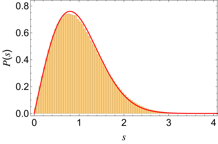
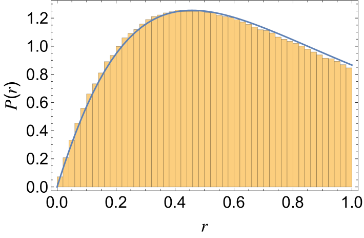
Figure 20: Level spacing statistics (left panel) and $r$-parameter statistics (right panel) for 1000 realizations of the Hamiltonian (57) with parameters $(h_{x},h_{z},g)=(-1.05,0.5,0.2)$, $s=1$, and $L=7$. The average $r$-parameter obtained is $\langle\tilde{r}\rangle=0.53$. The red and blue curves represent the Wigner-Dyson distributions for level spacing and $r$-parameter, respectively, corresponding to the $\nu=1$ (GOE). The analysis focuses on the central 50% of the spectrum, excluding the outermost 25% on each edge.

5.1 Approximate emergence of asymptotic freeness

In the spin-1 case, the fundamental operators of the theory, such as $X^{(s)}_{i}$, and their time-evolved counterparts, $X^{(s)}_{i}(t)$, have spectra characterized by a generalized Bernoulli distribution with eigenvalues $\pm\sqrt{3/2},0$. For convenience, we rescale these operators by a factor of $\sqrt{2/3}$, ensuring their spectra become $\pm 1,0$. As shown in Section 3.2 (Example 2), the free probability prediction for the spectrum of the sum of two free variables with generalized Bernoulli distribution with eigenvalues $\pm 1,0$ is given by Eq. (39). Figure 21 shows the spectrum of eigenvalues of the operator $\sqrt{2/3}(Z_{1}(0)+Z_{1}(t))$ with increasing time for 100 realizations of the Hamiltonian (57) at the chaotic point. The distribution predicted by free probability theory (39) becomes evident around $t=5$.

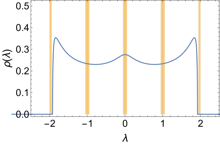
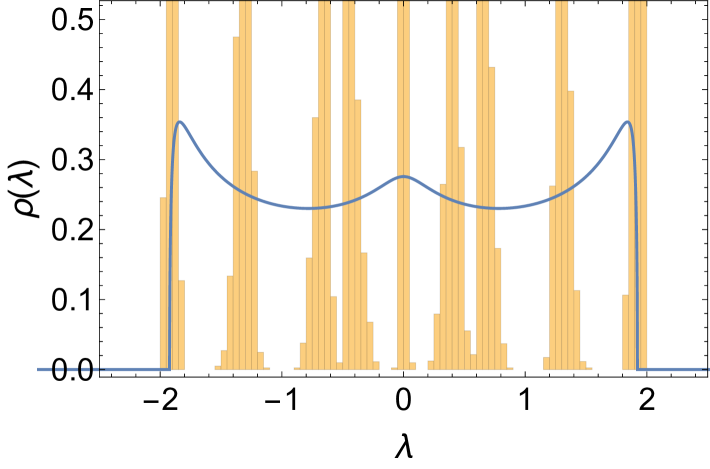
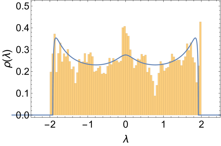
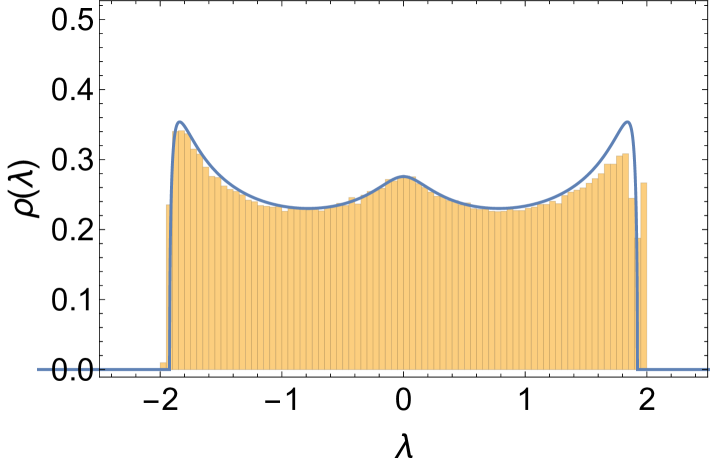
Figure 21: Evolution of the eigenvalue spectrum of the operator $\sqrt{2/3}(Z^{(s)}_{1}(0)+Z^{(s)}_{1}(t))$ with increasing time at the chaotic point. The parameters are fixed as $(h_{x},h_{z},g)=(-1.05,0.5,0.2)$, $s=1$, and $L=6$, with 100 realizations of the Hamiltonian (57). The distribution predicted by free probability theory (39) (depicted by the blue continuous line) becomes evident around $t=5$. The number of bins in each histogram is $100$.

5.2 Fluctuations

In this subsection, we investigate the fluctuations in the spectrum of the sum of spin-1 operators of the form $A+B(t)$. In the presence of chaotic dynamics, the operators $A$ and $B(t)$ are expected to become asymptotically free, with the distribution of their sum given by Eq. (39). The results are presented in Figures 22, 23, and 24. In all cases, we consider 100 realizations of the Hamiltonian (57) at the chaotic point $(h_{x},h_{z},g)=(-1.05,0.5,0.2)$, with $s=1$, $L=6$, and $t=50$.

$Z$-operators.

The results for the operator $\sqrt{2/3}(Z_{1}^{(s)}+Z_{6}^{(s)}(t))$ are shown in Figure 22. The left panel illustrates that the free probability prediction agrees well with the data, except for a deviation near the right edge of the spectrum. The right panel shows that the corresponding $r$-parameter distribution is well described by a Wigner $r$-parameter distribution with $\nu=2$.

$Y$-operators.

Figure 23 presents the results for the operator $\sqrt{2/3}(Y_{1}^{(s)}+Y_{6}^{(s)}(t))$. In this case, the free probability prediction provides an excellent fit across the entire spectrum, and the fluctuations are also well captured by random matrix theory with $\nu=2$.

$X$-operators.

The results for the operator $\sqrt{2/3}(X_{1}^{(s)}+X_{6}^{(s)}(t))$ are displayed in Figure 24. Here, while the overall shape of the curve follows the free probability prediction, quantitative discrepancies are observed. Nonetheless, the fluctuations remain well described by random matrix theory with $\nu=2$.

The key takeaway from this section is that, although the level spacing statistics of the model at the chaotic point are well described by random matrix theory, the free probability prediction for the sum of operators at different times holds only approximately, with deviations that depend on the specific choice of operators. In particular, the above results suggest that finite-size effects on the mixed cumulants in the model (57) are operator-dependent, with larger residual values observed for cumulants involving the $X$-operators, similar to what occurs in the spin chain model with $s=1/2$.

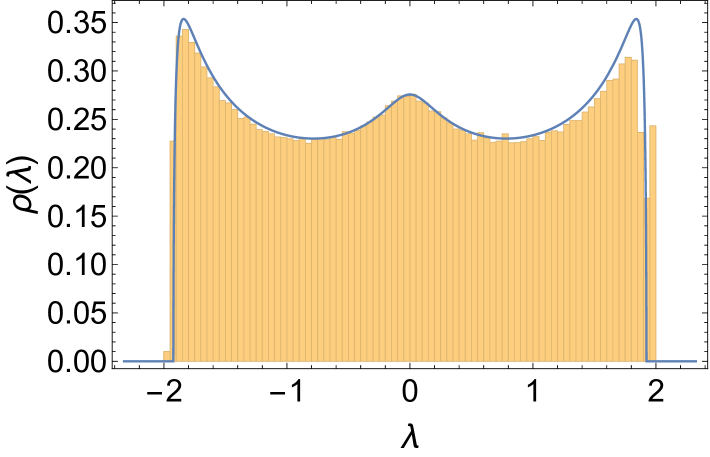
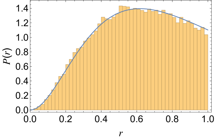
(a) Eigenvalue density	(b) $r$-parameter distribution

Figure 22: Spectral statistics of the operator $\sqrt{2/3}(Z_{1}^{(s)}+Z_{6}^{(s)}(t))$ based on 100 realizations of the Hamiltonian (57) at the chaotic point $(h_{x},h_{z},g)=(-1.05,0.5,0.2)$, with $s=1$, $L=6$ and $t=50$. The solid lines represent (a) the free probability prediction and (b) the Wigner $r$-parameter distribution for $\nu=2$. The $r$-parameter distribution was fitted using the form (83), yielding the Wigner parameter $\nu=1.999\pm 0.004$. The average $r$-parameter was found to be $\langle\tilde{r}\rangle=0.60$. The analysis focuses on the central 50% of the spectrum, excluding the outermost 25% on each edge.

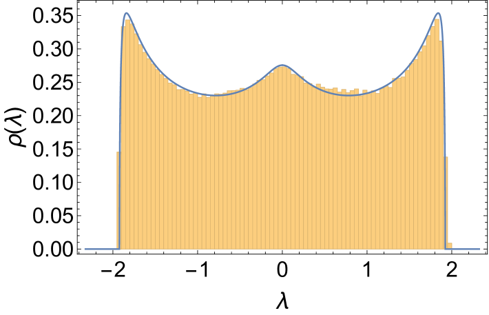
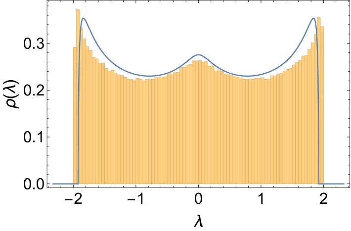
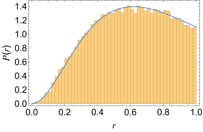
(a) Eigenvalue density	(b) $r$-parameter distribution

Figure 23: Spectral statistics of the operator $\sqrt{2/3}(Y_{1}^{(s)}+Y_{6}^{(s)}(t))$ based on 100 realizations of the Hamiltonian (57) at the chaotic point $(h_{x},h_{z},g)=(-1.05,0.5,0.2)$, with $s=1$, $L=6$ and $t=50$. The solid lines represent (a) the free probability prediction and (b) the Wigner $r$-parameter distribution for $\nu=2$. The $r$-parameter distribution was fitted using the form (83), yielding the Wigner parameter $\nu=2.000\pm 0.004$. The average $r$-parameter was found to be $\langle\tilde{r}\rangle=0.60$. The analysis focuses on the central 50% of the spectrum, excluding the outermost 25% on each edge.

(a) Eigenvalue density	(b) $r$-parameter distribution

Figure 24: Spectral statistics of the operator $\sqrt{2/3}(X_{1}^{(s)}+X_{6}^{(s)}(t))$ based on 100 realizations of the Hamiltonian (57) at the chaotic point $(h_{x},h_{z},g)=(-1.05,0.5,0.2)$, with $s=1$, $L=6$ and $t=50$. The solid lines represent (a) the free probability prediction and (b) the Wigner $r$-parameter distribution for $\nu=2$. The $r$-parameter distribution was fitted using the form (83), yielding the Wigner parameter $\nu=2.000\pm 0.004$. The average $r$-parameter was found to be $\langle\tilde{r}\rangle=0.60$. The analysis focuses on the central 50% of the spectrum, excluding the outermost 25% on each edge.

6 Asymptotic Freeness in the Sachdev–Ye–Kitaev Model

Finally, we discuss the emergence of asymptotic freeness in the SYK model. We consider the Hamiltonian of the standard $q=4$ SYK model with $N$ Majorana fermions, given by SachdevYeModel ; Kitaev2015

$$H_{\text{SYK}_{4}}=\sqrt{\frac{6}{N^{3}}}\sum_{j<k<l<m}J_{jklm}\,\psi_{j}\psi_{k}\psi_{l}\psi_{m}$$ (60)

where $\{\psi_{j},\psi_{k}\}=\delta_{jk}$, and $J_{jklm}$ is a random Gaussian variable with zero mean and standard deviation $J$.

The Hamiltonian (60) conserves charge parity, defined as $Q\mod 2$, where the charge operator $Q$ is expressed in terms of Dirac fermions $c_{i}$ as:

$$Q=\sum_{i=1}^{\left\lfloor N/2\right\rfloor}\bar{c}_{i}c_{i}\,.$$ (61)

where$\left\lfloor N/2\right\rfloor$ denotes the largest integer less than or equal to $N/2$. The Dirac fermions are related to the Majorana fermions by the transformations:

$$\psi_{2i}=\frac{c_{i}+\bar{c}_{i}}{\sqrt{2}}\,,\quad\psi_{2i-1}=\frac{i(c_{i}-\bar{c}_{i})}{\sqrt{2}}\,.$$ (62)

As a result, the Hamiltonian (60) can be cast into a block diagonal form, consisting of two blocks corresponding to positive and negative charge parity sectors Cotler:2016fpe . By representing the Majorana fermions in the chiral basis Pais1962 :

$$\psi_{i}=\frac{1}{\sqrt{2}}\begin{cases}\bigotimes_{k=1}^{\nu}\sigma_{1}&\text{if }i=1,\\[10.0pt] \left(\bigotimes_{k=1}^{\nu-\left\lfloor\frac{i}{2}\right\rfloor}\sigma_{1}\right)\otimes\sigma_{2}\otimes\left(\bigotimes_{k=1}^{\left\lfloor\frac{i}{2}\right\rfloor-1}\sigma_{0}\right)&\text{if }2\leq i\leq 2\nu\text{ and }i\text{ is even},\\[10.0pt] \left(\bigotimes_{k=1}^{\nu-\left\lfloor\frac{i-1}{2}\right\rfloor}\sigma_{1}\right)\otimes\sigma_{3}\otimes\left(\bigotimes_{k=1}^{\left\lfloor\frac{i-1}{2}\right\rfloor-1}\sigma_{0}\right)&\text{if }3\leq i\leq 2\nu\text{ and }i\text{ is odd},\\[10.0pt] \sigma_{2}\otimes\left(\bigotimes_{k=1}^{\nu-1}\sigma_{0}\right)&\text{if }i=2\nu.\end{cases}$$ (63)

the Hamiltonian (60) naturally assumes this block diagonal structure.

It is well known that the Hamiltonian (60) has level spacing statistics described by random matrix theory Garcia-Garcia:2016mno ; Garcia-Garcia:2017pzl . Figure 25 shows the level spacing statistics and the $r$-parameter statistics for this model for $N=16$, in which case the spectral statistics follow that of GOE of random matrices Cotler:2016fpe .

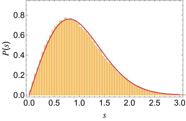
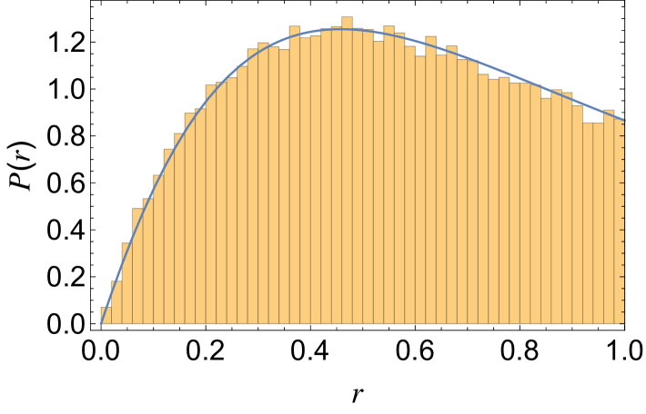
Figure 25: Level spacing statistics (left panel) and $r$-parameter statistics (right panel) for 1000 realizations of the Hamiltonian (60) with parameters $J=1$ and $N=16$. The average $r$-parameter obtained is $\langle\tilde{r}\rangle=0.53$. The red and blue curves represent the Wigner-Dyson distributions for level spacing and $r$-parameter, respectively, corresponding to $\nu=1$ (GOE). The analysis considers the full spectrum.

Figures 26 and 27 show the behavior of the spectral statistics for two choices of operator, $\sqrt{2}\left(\psi_{1}+\psi_{1}(t)\right)$ and $\sqrt{2}\left(\psi_{1}+\psi_{5}(t)\right)$ for different times. In both cases, the arcsine law emerges for timescales $t\sim O(10^{1})$.

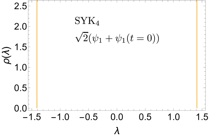
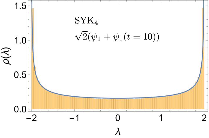
Figure 26: Spectral statistics (eigenvalue density) of the operator $\sqrt{2}\left(\psi_{1}+\psi_{1}(t)\right)$ for $1000$ realizations of the SYK₄ Hamiltonian (60), without fixing a chirality sector, with $N=16$ fermions for different times, indicated in each individual figure. The number of bins in each histogram is $100$.

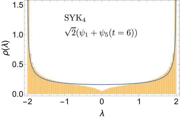
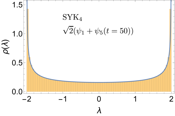
Figure 27: Spectral statistics (eigenvalue density) of the operator $\sqrt{2}\left(\psi_{1}+\psi_{5}(t)\right)$ for $1000$ realizations of the SYK₄ Hamiltonian (60), without fixing a chirality sector, with $N=16$ fermions for different times, indicated in each individual figure. The number of bins in each histogram is $100$.

To illustrate integrable dynamics, we also consider the integrable $q=2$ SYK Hamiltonian:

$$H_{\text{SYK}_{2}}=\frac{i}{\sqrt{N}}\sum_{j<k}K_{jk}\,\psi_{j}\psi_{k}$$ (64)

where $K_{jk}$ is drawn from a Gaussian distribution with zero mean and standard deviation $K$. In the chiral basis, the Hamiltonian (64) also takes a block diagonal form.

Figures 28 and 29 show the behavior of the spectral statistics for the two choices of the operator as in the SYK₄ case above, $\sqrt{2}\left(\psi_{1}+\psi_{1}(t)\right)$ and $\sqrt{2}\left(\psi_{1}+\psi_{5}(t)\right)$, for different times. In both cases, the arcsine law never emerges, at least within timescales up to order $t\sim O(10^{6})$.

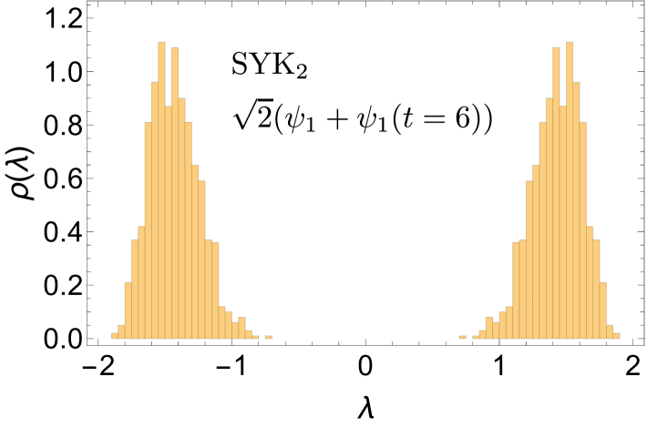
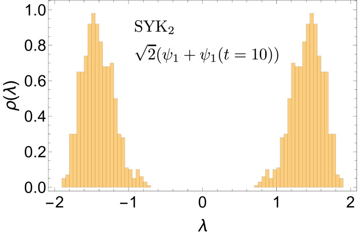
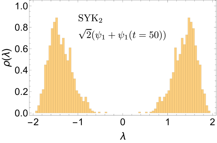
Figure 28: Spectral statistics (eigenvalue density) of the operator $\sqrt{2}\left(\psi_{1}+\psi_{1}(t)\right)$ for $1000$ realizations of the SYK₂ Hamiltonian (64), without fixing a chirality sector, with $N=16$ fermions for different times, indicated in each individual figure. The number of bins in each histogram is $100$. The acrsine distribution does not form, at least within timescales up to order $t\sim O(10^{6})$.

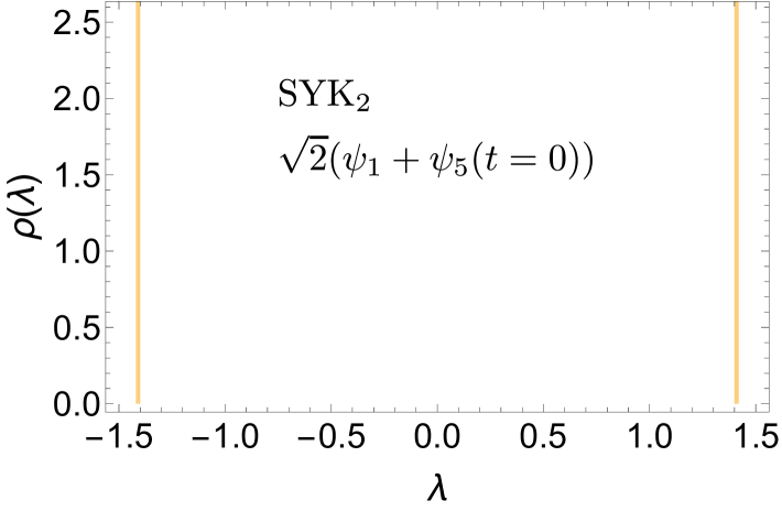
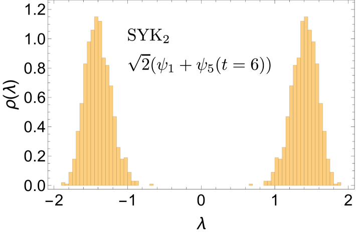
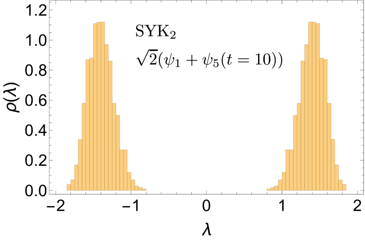
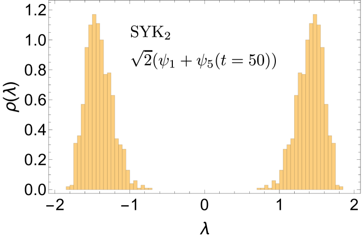
Figure 29: Spectral statistics (eigenvalue density) of the operator $\sqrt{2}\left(\psi_{1}+\psi_{5}(t)\right)$ for $1000$ realizations of the SYK₂ Hamiltonian (64), without fixing a chirality sector, with $N=16$ fermions for different times, indicated in each individual figure. The number of bins in each histogram is $100$. The arcsine distribution does not form, at least within timescales up to order $t\sim O(10^{6})$.

7 Conclusions and discussions

In this work, we argue that free probability theory provides the correct mathematical framework to describe quantum chaos. Beyond offering new tools to characterize quantum chaotic behavior, it also serves as a bridge connecting different manifestations of chaos in quantum systems.

We began by reviewing classical and quantum ergodic theories, emphasizing the probability spaces on which these theories are based. We then explored how different degrees of chaoticity can be quantified through the extent to which future operators, denoted by $B(t)$, become independent of past operators, $A(0)$. In free probability theory, statistical independence between two operators is encapsulated by the concept of freeness, which is defined by the vanishing of all mixed free cumulants involving $A(0)$ and $B(t)$ (see Eq.(16)). This property implies that mixed correlators involving $A(0)$ and $B(t)$ can be factorized in terms of products of their individual moments (see Sec.3.1).

Strictly speaking, freeness can only be realized for operators belonging to type III von Neumann algebras, which may emerge in the thermodynamic limit, $\mathcal{D}\to\infty$, where $\mathcal{D}$ denotes the matrix rank of the operators in the algebra or, equivalently, the dimension of the Hilbert space. For finite-dimensional systems, the algebra of operators is always type I, which does not allow strict mixing. In such cases, mixed cumulants in chaotic systems do not vanish at large times but instead approach a small non-zero value that decreases with increasing $\mathcal{D}$. This leads to the notion of asymptotic freeness, where cumulants vanish only in the limit $\mathcal{D}\to\infty$.

The spectral properties of asymptotically free operators provide a useful probe for quantum chaos. In particular, free probability theory predicts the eigenvalue distributions of combinations of asymptotically free operators. This prediction serves as a benchmark for testing the emergence of approximate asymptotic freeness in finite-dimensional quantum many-body systems under time evolution. Consequently, the spectral statistics of operators can be leveraged to test for asymptotic freeness.

Given two deterministic matrices $A$ and $B$, and a Haar-random unitary matrix $U$, it can be shown that $A$ and $U^{\dagger}BU$ are asymptotically free in the large-$\mathcal{D}$ limit with respect to the map $\varphi_{\mathcal{D}}(\cdot)$ (19), where $\mathbb{E}$ denotes the appropriate ensemble average over the unitary $U$. Since a strongly chaotic dynamics can often be approximated by replacing the time evolution operator with a Haar-random unitary, it is natural to expect that, in realistic Hamiltonians appearing in quantum many-body physics, strong chaos would lead to $A(0)$ and $B(t)$ becoming asymptotically free with respect to the state $\varphi_{\mathcal{D}}(\cdot)$ with $\mathbb{E}$ denoting an average over possibles random parameters in the Hamiltonian; or $\varphi_{\mathcal{D}}(\cdot)={\rm Tr}\,(\cdot)/\mathcal{D}$ if the Hamiltonian does not contain any random parameters. In this case, a smoking gun of asymptotic freeness is the spectral statistics of $A(0)+B(t)$ following the free convolution prediction.

As can be seen from eq. (16), the condition that defines two free operators depends on the map $\varphi(\cdot):\mathcal{A}\rightarrow\mathbb{C}$. Since, for a quantum system, this map essentially represents the state of the system, whether two quantum operators are free with respect to each other depends on this state. The primary quantity we have used in this paper as a signature of asymptotic freeness of two deterministic operators ($A$ and $B$) under time evolution, namely the spectral statistics of an operator of the form $A(0)+B(t)$, refers to a specific state of the quantum system for which the map acts as $\varphi(\cdot)=\mathbb{E}\left({\rm Tr}\,(\cdot)/\mathcal{D}\right)$. For a generic quantum system, this map would essentially represent an expectation value taken with respect to the infinite temperature thermal density matrix. Therefore, the observation that for chaotic systems, the eigenvalue density of $A(0)+B(t)$ starts to closely mimic the free convolution prediction around scrambling time is a strong indication that $A(0)$ and $B(t)$ indeed become asymptotically free under time evolution with respect to the above map.

The above discussion raises the question of whether we can test asymptotic freeness with respect to some other quantum state, say a finite temperature density matrix, in a similar way. As argued above, since the free probability prediction of the eigenvalue distribution of an operator of the form $A(0)+B(t)$ makes use of a specific instance of the map $\varphi(\cdot)$, in our opinion the eigenvalue distribution of $A(0)+B(t)$ is not a suitable quantity for that purpose. However, it would be interesting to look for other measures that might be useful in that context.

In the rest of this work, we performed a systematic study of the spectral statistics of the eigenvalues of operators of the form $A(0)+B(t)$ in various quantum many-body systems, including the mixed-field Ising model with a random magnetic field, a higher-spin generalization of this model, and the SYK model. We analyzed the timescale at which $A(0)$ and $B(t)$ become approximately free by comparing the eigenvalue distribution of $A(0)+B(t)$ with the predictions of free probability theory, which we also obtain in closed analytic form. Additionally, we investigated fluctuations on top of the free probability prediction by studying the level-spacing statistics of the eigenvalues of $A(0)+B(t)$. We now present a discussion of our results, contrasting the behavior in chaotic, near-integrable, and integrable regimes in the sense of nearest-neighbor level spacing statistics.

Chaotic cases.

For both the spin-1/2 and spin-1 Ising models with a random magnetic field, the eigenvalue density of operators of the form $A(0)+B(t)$ follows the free convolution prediction at times around the scrambling time. While this prediction accurately describes the eigenvalue density for some operators, others exhibit small deviations, particularly near the edges of the spectrum. A possible explanation for these deviations lies in the nature of spectral correlations in these models. They exhibit random matrix behavior in terms of nearest-neighbor level spacing statistics, which primarily capture short-range correlations between adjacent energy levels. However, full random matrix behavior, which ensures the emergence of free probability spectral prediction, requires more than just nearest-neighbor statistics. If the system deviates from random matrix behavior at longer energy level correlations, this could account for the observed discrepancies. To quantify these deviations and their impact on the emergence of free probability predictions, it would be interesting to analyze the $k$-th level spacing statistics Shir:2023olc in these models and compare them with the corresponding random matrix expectations.

In the SYK₄ model, the spectra of operators of the form $\psi_{i}(0)+\psi_{j}(t)$ are presented in Figures 26 and 27 for the cases $i=j=1$ and $i=1,j=5$, respectively. In both cases, the eigenvalue density converges to the arcsine law, the free probability prediction in this context, for times around $t\approx 10$. This indicates that the operators $\psi_{i}(0)$ and $\psi_{j}(t)$ become asymptotically free on this timescale. Notably, unlike the spin chain cases – where certain operators exhibit slight deviations from the free probability prediction – the SYK₄ model shows no such discrepancies. This confirms the expectation that the SYK₄ model is more chaotic than the spin chain models considered in this work.

The emergence of the free probability prediction in the SYK₄ model at finite $N$ suggests that the model satisfies the F-property in the limit $N\to\infty$. Since the F-property implies mixing, which typically requires a type III algebra, this provides strong evidence that the corresponding algebra of observables becomes type III in this limit, in agreement with expectations from the literature Leutheusser:2021frk .

Near-integrable cases.

Previous works suggest that the free convolution prediction for the spectrum of operators of the form $A+B(t)$ holds even in systems near integrability Chen:2024zfj , albeit emerging at significantly longer times compared to fully chaotic cases. However, increasing the statistical sampling reveals deviations from the free convolution prediction for the $X$ Pauli operators, whereas no such deviations are observed for the $Z$ Pauli operators (see Sec. 4.3). This suggests that, near the integrable point, $Z_{i}(0)$ and $Z_{j}(t)$ remain asymptotically free at sufficiently large times, while $X_{i}(0)$ and $X_{j}(t)$ do not. Such an operator-dependent asymptotic freeness could be a distinctive feature of near-integrable systems. In the next subsection, we outline a strategy to investigate whether this is indeed the case.

For the mixed-field Ising model, we also investigate how the timescale at which the arcsine law emerges varies as the system is driven from the chaotic regime toward integrability. More specifically, we analyze how the arcsine time depends on the average $r$-parameter, with the results presented in Figure 15. We observe that the arcsine time increases as $r$ decreases from its GOE value of approximately 0.53, eventually diverging as the system approaches integrability. Indeed, we verified that at the precisely integrable point, the arcsine law never emerges, regardless of how large we set the time.

Integrable cases.

In SYK₂, the spectra of operators of the form $\psi_{i}(0)+\psi_{j}(t)$ are shown in Figures 28 and 29 for the cases $i=j=1$ and $i=1,j=5$, respectively. We observe that, regardless of how large the time parameter is, the arcsine law never emerges. As observed before, the same happens at the integrable point of the mixed-field Ising model.

Fluctuations and symmetry resolution.

In the spin-chain models we considered, the random magnetic field breaks parity symmetry, leaving energy as the only conserved quantity. Consequently, there is no need to account for distinct symmetry sectors. Symmetry resolution techniques are typically employed when analyzing spectral fluctuations, which suggests that in systems with conserved charges, symmetry resolution plays a crucial role in accurately capturing fluctuations beyond the predictions of free probability. However, it seems to be less relevant for determining whether the eigenvalue density follows free probability predictions.

For spin chains, we analyzed the $r$-parameter statistics associated with spectral fluctuations and found that they are well described by the Wigner-Dyson distribution with either $\nu=1$ or $\nu=2$. Specifically, for the sum of operators at different sites, we observe a GUE-type distribution ($\nu=2$), whereas for operators acting on the same site, the statistics follow a GOE-type distribution ($\nu=1$). The emergence of GUE-type statistics in the former case can be attributed to the breaking of time-reversal symmetry.

For the SYK model in the chiral basis, the Hamiltonian takes a block-diagonal form, corresponding to the two charge-parity sectors of the model. The analysis of fluctuations in this case should account for these two symmetry sectors. Operators of the form $\psi_{i}(0)+\psi_{j}(t)$ take an off-diagonal block form, with each block presumably corresponding to one of the charge-parity sectors. However, each block results in a matrix that is not Hermitian. It is not yet entirely clear to us how to perform the level spacing or $r$-parameter statistics in this case, so we leave this for future work.

Previous Works Connecting Different Notions of Quantum Chaos.

Finally, we comment on previous works that connect different notions of quantum chaos. In Cotler:2017jue , the authors establish a connection between correlators involving Haar random unitary operators and a generalized version of the spectral form factor (see Appendix D for a brief review). Specifically, they show that higher-order OTOCs involving Haar random unitaries are related to the $k$-th power of the spectral form factor, thus linking the vanishing of OTOCs with spectral statistics exhibiting random matrix behavior. In contrast, the concept of freeness between operators $A(0)$ and $B(t)$ encompasses the vanishing of all mixed free cumulants, including two-point functions, OTOCs, and higher-order out-of-time-ordered correlators. If the time evolution operator is modeled by a Haar random unitary $U$, one can show that $A(0)$ and $U^{\dagger}BU$ are asymptotically free, implying the vanishing of all mixed free cumulants. In this case, an ensemble average is taken in the definition of the map $\varphi(A)=\lim_{\mathcal{D}\rightarrow\infty}\mathbb{E}\left(\frac{{\rm Tr}\,A}{\mathcal{D}}\right)$.

Another relevant work connecting OTOCs with operator spectral statistics is rozenbaum2019universal , which argues that in chaotic systems, out-of-time-order operators (OTOOs) of the form $A(0)B(t)A(0)B(t)+B(t)A(0)B(t)A(0)$ display universal level spacing statistics. In free probability, the fact that $A(0)$ and $B(t)$ become asymptotically free under chaotic dynamics should allow one to obtain the free probability prediction for the eigenvalue density of the OTOO mentioned above. In the next section, we elaborate on how to proceed in this direction of research.

7.1 Future directions

This work can be extended in several interesting directions, some of which we now briefly discuss.

• In this work, we have examined the free convolution prediction for the sum of two free operators, focusing on spin-1/2 and spin-1 operators. While these results, specially, the spin-1/2 case, apply to a broad class of quantum mechanical systems, including spin chains and SYK-like models, it is crucial to extend the free convolution prediction to sums of other types of operators that naturally arise in quantum mechanics. In Sec. 3.2.1, we numerically determine the free additive convolution for the sum of two free spin-3/2, spin-2 and spin-5/2 operators as a first step in this direction. However, many important cases remain unexplored, such as bosonic operators in, say, the Bose-Hubbard model, and the position $x$ and momentum $p$ operators in quantum billiard systems, and numerous others. A systematic classification of free convolution predictions for different classes of operators would be highly valuable for future studies on quantum chaos and asymptotic freeness in quantum mechanics.

• The approximate validity of the free convolution prediction for systems near integrability, when considering the $Z$ Pauli operators, suggests that even a slight breaking of integrability could lead to mixing in the thermodynamic limit for cumulants involving these operators. A natural way to investigate this would be to analyze the scaling of the residual value of mixed free cumulants with $N$ in systems with an intermediate degree of chaos. This would extend the numerical studies of Huang:2017fng , which focused on strongly chaotic systems, to such intermediate cases.

• In this paper we have considered spectral properties of the sum of two non-commutative operators (say $A$ and $B$). However, one can similarly consider the spectral properties of the products of two such operators, as well as their different linear combinations. If these variables are traceless, i.e., $\varphi(A)=\varphi(B)=0$, then their free product is trivial since the trace of a combination of them vanishes from the definition freeness, $\varphi\big{(}(AB)^{k}\big{)}=\varphi\big{(}ABAB\cdots AB\big{)}=0$. For variables with non-zero trace, one can obtain the free multiplicative convolution of these variables by using an analogue of the $R$-transform, known as the $S$-transform, which has the property that for a pair of free variables, it is multiplicative voiculescu1987multiplication . This allows us to compute the free multiplicative convolution of the eigenvalue density of these two operators and obtain the eigenvalue density of the product by using the rule $S_{\rho_{A}\boxtimes\rho_{B}}(x)=S_{\rho_{A}}(x)S_{\rho_{B}}(x)$. A particular set of combinations of addition and multiplication of two non-commutative variables that are relevant for our purposes is the squared commutator $(-i)^{2}\big{[}A(t),B(0)\big{]}^{2}$ and its higher-order generalizations. If $A(t)$ and $B(0)$ are asymptotically free, a prediction for the spectral statistics of this operator would help us to understand, in precise terms, the connection between previous proposals regarding the spectral statistics of out-of-time-order operators and the Lyapunovian operator rozenbaum2019universal , and the emergence of asymptotic freeness in chaotic quantum many-body dynamics that we have advocated here.

• It would be interesting to investigate the role of freeness in quantum field theories (QFTs). Notably, freeness imposes nontrivial constraints on these theories. In two-dimensional integrable conformal field theories (CFTs), for instance, two-point functions exhibit universal behavior, always decaying to zero as $t\to\infty$. However, four-point OTOCs depend on the choice of operators: they remain constant when involving only energy operators or a combination of energy and spin operators. In contrast, chaotic CFTs display a more uniform decay, where both two-point functions and OTOCs tend to zero for almost any choice of operators, and higher-order OTOCs are also expected to vanish at late times (see Appendix B of Roberts:2014ifa ).

  Moreover, it would be valuable to study operator spectral statistics in interacting QFTs using light-cone truncation methods Delacretaz:2022ojg .

• It is crucial to determine the precise position of the notion of freeness (F-property) within the quantum ergodic hierarchy. We hypothesize that it lies between mixing and $K$-mixing, but further investigation is required to determine whether this is indeed true. Furthermore, exploring the relationship between $K$-mixing, the existence of quantum Lyapunov exponents, and stronger notions of freeness, such as second-order freeness collins2024second , is an important direction for future research.

• Recently, a new manifestation of quantum chaotic behavior was identified in the BPS sectors of supersymmetric theories, a phenomenon referred to as “BPS chaos” Chen:2024oqv . The procedure begins with an operator $\mathcal{O}$ in the UV theory, which is then projected into a BPS sector via $\mathcal{O}_{\text{BPS}}=P_{\text{BPS}}\mathcal{O}P_{\text{BPS}}$, where $P_{\text{BPS}}$ is a projection operator, morally taking the form $P_{\text{BPS}}=\lim_{\beta\rightarrow\infty}e^{-\beta H}$. For BPS sectors dual to black hole geometries, one expects to observe random matrix behavior upon studying the spectral properties of $\mathcal{O}_{\text{BPS}}$. It would be interesting to investigate whether this new manifestation of quantum chaos can be derived from free probability, as a consequence of the free independence between the operator $\mathcal{O}$ and the projector $P_{\text{BPS}}$.

We look forward to reporting on these developments in future work.

Appendix A Cumulants from partitions

In this appendix we provide a brief introduction to the free cumulants associated with non-commutating random variables, starting from the standard definition of the classical cumulants of commutating random variables. We discuss the diagrammatic method based on crossing and non-crossing partitions of a set to obtain the classical and free cumulants, which has been used recently to connect the eigenstate thermalization hypothesis and the dynamics of fluctuations of coherence in noisy mesoscopic systems with the free probability theory Pappalardi:2022aaz ; Hruza:2022uqj . For more detail on the combinatorics in free probabilities, we refer to speicher2009free ; speicher2019lecture ; mingo2017free ; nica2006lectures ; Potters .

Consider an algebra of random variables $\mathcal{R}$, and a positive faithful linear functional $\varphi(\cdot)$ which maps $\mathcal{R}\rightarrow\mathbb{C}$. Usual examples of this functional include the expectation operator ($\mathbb{E}[\cdot]$) in standard probability theory, or the (normalized) trace operator ${\rm Tr}\,(\cdot)/N$ for an algebra of matrices, or it could be a combination of these two operations, $\mathbb{E}[\text{Tr}(\cdot)]/N$.

(a) $n=1$

(b) $n=2$

(c) $n=3$

(d) $n=4$

Figure 30: Diagrams for partitions of a set used to obtain the classical and free cumulants. All the partitions contribute to classical cumulants, while only the non-crossing partitions contribute to free cumulants. Crossing partitions start to appear from $n=4$ onward (distinguished above from the non-crossing ones by red lines).

Commutating random variables: Classical cumulants. We start by considering the cumulants of commutating random variables, known as the classical cumulants $c_{n}(x)$. These are essentially the connected correlation functions of the random variables of different orders and can be conveniently written as combinations of $n$-th order and lower order moments $m_{n}=\varphi(x^{n})$. One can obtain the relation between the first few moments and cumulants straightforwardly from their respective generating functions. We start from the cumulant generating function $K(x)=\sum_{n}c_{n}x^{n}/n!$, which is related with the moment generating function $G(x)$ as

$$G(x)=e^{K(x)}=\sum_{n}m_{n}x^{n}/n!~.$$ (65)

Taking successive derivatives of the relation between the first few moments and cumulants are given by

$$m_{1} =\frac{d}{dx}\big{(}e^{K(x)}\big{)}\Big{|}_{x=0}=c_{1}$$

$$m_{2} =\frac{d^{2}}{dx^{2}}\big{(}e^{K(x)}\big{)}\Big{|}_{x=0}=e^{K(x)}\Big{(}K^{\prime}(x)^{2}+K^{\prime\prime}(x)\Big{)}\Big{|}_{x=0}=c_{1}^{2}+c_{2}$$

$$m_{3} =\frac{d^{3}}{dx^{3}}\big{(}e^{K(x)}\big{)}\Big{|}_{x=0}=e^{K(x)}\Big{(}K^{\prime}(x)^{3}+3K^{\prime}(x)K^{\prime\prime}(x)+K^{\prime\prime\prime}(x)\Big{)}\Big{|}_{x=0}=c_{1}^{3}+3c_{1}c_{2}+c_{3}$$

$$m_{4} =\frac{d^{4}}{dx^{4}}\big{(}e^{K(x)}\big{)}\Big{|}_{x=0}=e^{K(x)}\Big{(}K^{\prime}(x)^{4}+6K^{\prime}(x)^{2}K^{\prime\prime}(x)+4K^{\prime}(x)K^{\prime\prime\prime}(x)+3K^{\prime\prime}(x)^{2}$$

$$+K^{(4)}(x)\Big{)}\Big{|}_{x=0}=c_{1}^{4}+6c_{1}^{2}c_{2}+4c_{1}c_{3}+3c_{2}^{2}+c_{4}~.$$ (66)

Inverting these relations we obtain the expressions for the cumulants in terms of the moments

$$c_{1} =m_{1}$$

$$c_{2} =m_{2}-m_{1}^{2}$$

$$c_{3} =m_{3}-3m_{2}m_{1}+2m_{1}^{3}$$

$$c_{4} =m_{4}-4m_{1}m_{3}+12m_{2}m_{1}^{2}-3m_{2}^{2}-6m_{1}^{4}~.$$ (67)

These relations between the classical cumulants and the moments can be written compactly using the concept of partitions. For a set $\{1,\cdots n\}$, a partition $\pi$ represents a decomposition of the set in terms of blocks that do not overlap while the union of all these blocks gives back the full set. The set of all partitions of $\{1,2,\cdots n\}$ is denoted as $P(n)$. We have shown the set of all partitions for $n=1,2,3,4$ in Figure 30. Note that for $n=1,2,3$, all the partitions are non-crossing, while for $n=4$, there is one crossing partition (shown in red). The total number of partitions (crossing as well as non-crossing) of a set with $n$ elements is known as the Bell number ($B_{n}$), which satisfies the recurrence relations $B_{n+1}=\sum_{k=0}^{n}\Big{(}\begin{array}[]{c}n\\ k\end{array}\Big{)}B_{k}$. Then, the moments are related to the classical cumulants through the formula

$$m_{n}(x)=\sum_{\pi\in P(n)}c_{\pi}(x),~~\text{where}~~c_{\pi}(x)=\prod_{b\in\pi}c_{|b|}(x)~.$$ (68)

According to this formula, the quantity $c_{\pi}(x)$ is defined as the product of the cumulants over the number of the elements of the block $b$ of a certain partition $\pi$. As an example, consulting the partitions for $n=4$ shown in Fig. 30 it can be deduced that the fourth order moment is given in terms of the classical cumulants as $m_{4}(x)\equiv\mathbb{E}(x^{4})=c_{4}(x)+3c_{2}^{2}(x)+6c_{2}(x)c_{1}^{2}(x)+4c_{3}(x)c_{1}(x)+c_{1}^{4}(x)$, which is the same as the expression for $m_{4}$ we obtained in (A) by taking successive derivatives of the cumulant generating function. The formula in eq. (68) can be inverted for each $n$ to obtain the classical cumulants in terms of the moments.

Finally, for more than one random variable $(x_{1}x_{2}\cdots x_{n})$, the formula connecting the moments and the cumulants can be generalized to obtain

$$\mathbb{E}(x_{1}x_{2}\cdots x_{n})=\sum_{\pi\in P(n)}c_{\pi}(x_{1}x_{2}\cdots x_{n}),~~\text{where}~~c_{\pi}(x_{1}x_{2}\cdots x_{n})=\prod_{b\in\pi}c_{|b|}\Big{(}x_{b(1)}x_{b(2)}\cdots x_{b(n)}\Big{)}~.$$ (69)

Non-commutating random variables: Free cumulants. Now we consider the cumulants for non-commutating random variables ($A_{1},A_{2},\cdots A_{n}$), known as the free cumulants ($\kappa_{n}$). To relate these with $\phi(A^{n})$ we need to consider the partitions of the set $\{1,2,\cdots n\}$ which do not cross. While the total number of partitions of this set is given by the Bell numbers, the number of non-crossing partitions ($NC(n)$) is given by the Catalan numbers $C_{n}=\frac{1}{n+1}\Big{(}\begin{array}[]{c}2n\\ n\end{array}\Big{)}$, and the relation between $\phi(A^{n})$ and $\kappa_{n}$ of different order can be written as a sum over the non-crossing partitions in the following way,

$$\varphi(A^{n})=\sum_{\pi\in NC(n)}\kappa_{\pi}(A),~~\text{where}~~~~\kappa_{\pi}(A)=\prod_{b\in\pi}\kappa_{|b|}(A)~.$$ (70)

The expressions for the first four free cumulants are, therefore,

$$\kappa_{1} =\varphi(A)$$

$$\kappa_{2} =\varphi(A^{2})-\varphi(A)^{2}$$

$$\kappa_{3} =\varphi(A^{3})-3\varphi(A^{2})\varphi(A)+2\varphi(A)^{3}$$

$$\kappa_{4} =\varphi(A^{4})-4\varphi(A)\varphi(A^{3})+10\varphi(A^{2})\varphi(A)^{2}-2\varphi(A^{2})^{2}-5\varphi(A)^{4}~.$$ (71)

As can be expected from the partitions shown in Figure 30, the difference between the classical and free cumulants starts to appear for $n=4$, so that we have the relation $\varphi(A^{4})=\kappa_{4}(A)+2\kappa_{2}^{2}(A)+6\kappa_{2}(A)\kappa_{1}^{2}(A)+4\kappa_{3}(A)\kappa_{1}(A)+\kappa_{1}^{4}(A)$. For more than one random variable, we can extend the relation in eq. (70) to

$$\begin{split}\varphi(A_{1}A_{2}\cdots A_{n})=\sum_{\pi\in NC(n)}\kappa_{\pi}(A_{1},A_{2},\cdots A_{n})~,\\ \text{where}~~\kappa_{\pi}(A_{1},A_{2},\cdots A_{n})=\prod_{b\in\pi}\kappa_{|b|}\Big{(}A_{b(1)},A_{b(2)},\cdots A_{b(n)}\Big{)}~.\end{split}$$ (72)

Here $b$ denotes the different elements of the blocks of the partitions, $b=(b(1),b(2),\cdots b(n))$ and $|b|$ indicates its length.

Appendix B Details about the Level Spacing Analysis

The average density of states in a chaotic spectrum is typically dependent on the specific model and is non-universal. In contrast, it is conjectured that fluctuations around the average density of states can be accurately described by the random matrix theory corresponding to the appropriate symmetry class BGS ; BGS2 . Thus, it is crucial to isolate the spectral fluctuations from the average density of states. The standard method to achieve this is known as unfolding, which involves mapping the original energy levels $E_{n}$ to new levels $\epsilon_{n}$ that preserve the fluctuation properties while normalizing the average density of states to one. In this appendix, we provide a review of the unfolding process, using a chaotic spin chain as an illustrative example.

Consider the scenario where we directly diagonalize the Hamiltonian of a given system and obtain the energy spectrum $E_{n}$ within a particular symmetry sector. The initial step involves determining the average density of states, $\rho_{\text{avg}}(E)$.

After obtaining the average density of states, we compute the corresponding cumulative distribution function:

$$N_{\text{avg}}(E)=\int_{-\infty}^{E}\textrm{d}E^{\prime}\rho_{\text{avg}}(E^{\prime})\,.$$ (73)

The unfolding procedure is then defined by the mapping:

$$\varepsilon_{n}=N_{\text{avg}}(E_{n})\,.$$ (74)

The average density of states of the unfolded spectrum is very close to one. The nearest-neighbor level spacing distribution of the unfolded spectrum can then be obtained by computing the spacings:

$$s_{i}=\varepsilon_{i+1}-\varepsilon_{i}\approx\rho(E_{i})(E_{i+1}-E_{i})\,,$$ (75)

and constructing a histogram of $s_{i}$. For a sufficiently large number of spacings, one can obtain a good estimate of the level spacing distribution, $P(s)$. When this distribution resembles those observed in random matrix ensembles, the system is considered ’quantum chaotic’. In contrast, for many integrable systems, the energy levels are uncorrelated and follow Poisson statistics BerryTabor1977 .

The Wigner-Dyson distributions can be compactly written as:

$$P_{\nu}(s)=a(\nu)s^{\nu}e^{-b(\nu)s^{2}}\,,$$ (76)

where the constants $a(\nu)$ and $b(\nu)$ are determined by the conditions:

$$\int_{0}^{\infty}P_{\nu}(s)\textrm{d}s=1\,,\,\,\,\,\,\,\int_{0}^{\infty}s\,P_{\nu}(s)\textrm{d}s=1\,.$$ (77)

The index $\nu$ specifies the symmetry class of the random matrix ensemble, with $\nu=1$ for GOE, $\nu=2$ for GUE, and $\nu=4$ for GSE. In these cases, the formula takes the following form:

$$P_{\nu}(s)=\begin{cases}\frac{\pi}{2}s\,e^{-\pi s^{2}/4},&\nu=1\,\,\text{(GOE)}\\ \frac{32}{\pi^{2}}s^{2}\,e^{-4s^{2}/\pi},&\nu=2\,\,\text{(GUE)}\\ \frac{2^{18}}{3^{6}\pi^{3}}s^{4}\,e^{-64s^{2}/(9\pi)},&\nu=4\,\,\text{(GSE)}\end{cases}$$ (78)

For a spectrum with uncorrelated energy levels, the level spacing distribution follows Poisson statistics:

$$P_{\text{Poisson}}(s)=e^{-s}\,.$$ (79)

One limitation of using the level spacing distribution to characterize random matrix behavior is the need to unfold the spectrum, which requires knowledge of the system’s average density of states. In the cases considered in this paper, the average density of states follows either a Wigner semicircle distribution (for SYK₄) or a Gaussian distribution (for spin chains), making the unfolding procedure straightforward. However, for models without an analytic formula for the average density of states (SYK₂ for example), the unfolding procedure becomes more complex and may introduce errors. Therefore, it is important to use alternative methods that do not require unfolding, reducing the risk of such errors. One such method is the $r$-parameter statistics, which we discuss in Appendix C.

Appendix C $r$-parameter statistics

In this Appendix, we discuss the statistics of the so-called $r$-parameter, which is essentially the distribution of the ratio of nearest-neighbour spacings, and therefore serves as an important tool for diagnosing the correlation in the energy spectrum. Within a symmetry sector of the system, consider an ordered spectrum ${E_{n}}$, and define the nearest-neighbour level spacings $s_{n}=E_{n+1}-E_{n}$. From these level spacings, we define the $r_{n}\equiv s_{n}/s_{n-1}$, and consider the distribution of the following quantity, known as the $r$-parameter Oganesyan:2007wpd

$$\tilde{r}_{n}\equiv\frac{\text{min}(s_{n},s_{n-1})}{\text{max}(s_{n},s_{n-1})}=\text{min}~\Big{(}r_{n},\frac{1}{r_{n}}\Big{)}~.$$ (80)

One of the most important advantages of studying the $r$-parameter is that one does not need to unfold the energy spectrum, and hence does not need to have knowledge of the local density of states, since the ratios of successive level spacings are independent of the local density of states. For an $N\times N$ random matrix Hamiltonian belonging to the classical Gaussian ensembles, the distribution of ratio $r$ is given by

$$P(r_{1},\dots,r_{N-2})=\left(\prod_{i=1}^{N}\int\textrm{d}E_{i}\right)P(E_{1},\dots,E_{N})\prod_{i=1}^{N-2}\delta\left(r_{i}-\frac{E_{i+2}-E_{i+1}}{E_{i+1}-E_{i}}\right)~,$$ (81)

where $P(E_{1},\dots,E_{N})$ denotes the joint probability distribution of the eigenvalues, which for the Gaussian ensembles under consideration is given by mehta1991random :

$$P(E_{1},\dots,E_{N})=C_{\nu,N}e^{-\frac{\nu N}{4}\sum_{k=1}^{N}E_{k}^{2}}\prod_{i<j}|E_{i}-E_{j}|^{\nu}~,$$ (82)

$C_{\nu,N}$ being a constant which normalizes the distribution.

An important result on the statistics of the $r$-parameter was obtained in Atas_2013 , where a Wigner-like surmise for the distribution of $r_{n}$ was obtained analytically for all three classical random matrix ensemble by considering a model of $3\times 3$ matrices. This expression, which already provides a very good approximation for the distribution of $P(r)$ obtained from exact numerical analysis of matrices of large sizes, is given by

$$P_{W}(r)=\frac{1}{Z_{\nu}}\frac{(r+r^{2})^{\nu}}{(1+r+r^{2})^{1+\frac{3}{2}\nu}}~,$$ (83)

where $Z_{\nu}$ is a normalization constant that depends on the Dyson index $\nu$. This distribution of $r$ has the similar level repulsion as that of the distribution of the level spacing for small values of $r$, i.e., $P_{W}(r)\sim r^{\nu}$. On the other hand, for large values $r$, unlike the distribution of level spacings, the $P_{W}(r)$ does not decay exponentially, rather it has slower polynomial decay, $P_{W}(r)\sim r^{-(2+\nu)}$.

From the above expression for the distribution of $r$, one can analytically calculate the average value of the $r$ parameter to be

$$\langle\tilde{r}\rangle_{W}=\int_{0}^{1}\textrm{d}r~rP_{W}(r)+\int_{1}^{\infty}\textrm{d}r~r^{-1}P_{W}(r)~.$$ (84)

We also note that, for an uncorrelated spectrum, with level spacing statistics following a Poisson distribution, the probability distribution of the ratio $r$ is given by:

$$P_{\text{Poisson}}(r)=\frac{2}{(1+r)^{2}}.$$ (85)

Numerically, one can calculate each of the individual $\tilde{r}$ parameter from eq. (80), and obtain the average using

$$\langle\tilde{r}\rangle=\frac{1}{N-1}\sum_{n=1}^{N-1}\tilde{r}_{n}\,.$$ (86)

Table 1 presents the average $r$-parameter for various random matrix ensembles, including the GOE, GUE, and Gaussian Symplectic Ensemble (GSE), as well as for a spectrum that follows Poisson statistics.

Table 1: Average $r$-parameter for different ensembles

Ensemble	$\langle r\rangle$
Poisson	$\approx 0.386$
GOE	$\approx 0.536$
GUE	$\approx 0.602$
GSE	$\approx 0.676$

Appendix D Average correlators and spectral form factor

In this appendix we review some relations between the averages of time-ordered and out-of-time-ordered correlation functions and the spectral form factor Cotler:2017jue . Specifically, the connections between the OTOC and the spectral form factor (SFF) we discuss can be thought of as a bridge between two different popular ways of quantifying quantum chaos.

We start by considering a generic system described by a Hamiltonian $H$, having Hilbert space dimension $L=2^{n}$, and a unitary operator $\mathcal{U}$. Using the formula for the first moment of the Haar ensemble associated with this operator, the average of the corresponding 2-point function over the Haar measure defined on $U(2^{n})$ can be related to the 2-point spectral form factor as,

$$\int\textrm{d}\mathcal{U}~\big{<}\mathcal{U}(t=0)\mathcal{U}^{\dagger}(t)\big{>}\equiv\frac{1}{L}\int\textrm{d}\mathcal{U}~\text{Tr}\big{[}\mathcal{U}e^{-iHt}\mathcal{U}^{\dagger}e^{-iHt}\big{]}\\ =\frac{1}{L^{2}}\big{|}\text{Tr}\big{[}e^{-iHt}\big{]}\big{|}^{2}~=\frac{1}{L^{2}}\mathcal{R}^{H}_{2}(t)~,$$ (87)

where $\mathcal{R}^{H}_{2}(t)$ denotes the 2-point form factor associated with the Hamiltonian $H$. This formula provides a direct way of estimating the spectral form factor from the knowledge of the 2-point function, since, the variance is suppressed by $1/L$, i.e. Cotler:2017jue ,

$$\Delta\big{<}\mathcal{U}(t)\mathcal{U}^{\dagger}(t)\big{>}^{2}_{\text{avg}}=\int\textrm{d}\mathcal{U}\big{|}\big{<}\mathcal{U}(0)\mathcal{U}^{\dagger}(t)\big{>}\big{|}^{2}-\bigg{|}\int\textrm{d}\mathcal{U}\big{<}\mathcal{U}(0)\mathcal{U}^{\dagger}(t)\big{>}\bigg{|}^{2}\sim\mathcal{O}(1/L^{2})~.$$ (88)

That the formula in eq. (87) is true, and the error is small were verified in Cotler:2017jue by numerical simulation of a random non-local spin system.

For an OTOC, defined for two unitary operators, an analogous computation using the first moment of the Haar ensemble gives a different type of form factor

$$\int\textrm{d}\mathcal{U}_{1}\textrm{d}\mathcal{U}_{2}~\big{<}\mathcal{U}_{1}(0)\mathcal{U}_{1}^{\dagger}(t)\mathcal{U}_{2}(0)\mathcal{U}_{2}^{\dagger}(t)\big{>}=\frac{1}{L^{3}}\text{Tr}\big{[}e^{-iHt}\big{]}^{2}\text{Tr}\big{[}e^{-2iHt}\big{]}~.$$ (89)

This identity can be easily generalized for $k$ different operators to get,

$$\int\textrm{d}\mathcal{U}_{1}\textrm{d}\mathcal{U}_{2}\cdots\textrm{d}\mathcal{U}_{k}~\big{<}\mathcal{U}_{1}(0)\mathcal{U}_{1}^{\dagger}(t)\cdots\mathcal{U}_{k}(0)\mathcal{U}_{k}^{\dagger}(t)\big{>}=\frac{1}{L^{k+1}}\text{Tr}\big{[}e^{-iHt}\big{]}^{k}\text{Tr}\big{[}e^{-kiHt}\big{]}~.$$ (90)

To obtain the $2k$-point form factor from an OTOC average, one can consider the following average of a $2k$-point OTOC, and using the first moment of the Haar ensemble $2k-1$ times obtain Cotler:2017jue ,

$$\int\textrm{d}\mathcal{U}_{1}\textrm{d}\mathcal{V}_{1}\cdots\textrm{d}\mathcal{V}_{k-1}\textrm{d}\mathcal{U}_{k}~\big{<}\mathcal{U}_{1}(0)\mathcal{V}_{1}(t)\cdots\mathcal{U}_{k}(0)\mathcal{V}_{k}(t)\big{>}=\frac{1}{L^{2k}}\big{|}\text{Tr}\big{[}e^{-iHt}\big{]}\big{|}^{2k}~=\frac{1}{L^{2k}}\mathcal{R}^{H}_{2k}(t)~.$$ (91)

To summarize, these relations connecting the averages of the time-ordered correlators and OTOC with various spectral form factors indicate that the spectral statistics can not capture either of the spatial and temporal locality of the operators.

Operator averages for random matrix Hamiltonians. The relations between the averages of the correlation function and the SFFs discussed above are valid for any arbitrary Hamiltonian. One can also derive similar such relations when the Hamiltonian is drawn from some random matrix ensemble and the average is performed over the ensemble. For instance, for a random matrix Hamiltonian taken from the GUE, utilizing the invariance of the integral measure under unitary transformations, the following relation can be established between the ensemble-averaged 2-point correlation function and the 2-point form factor of the ensemble Cotler:2017jue

$$\big{<}\mathcal{U}(0)\mathcal{V}(t)\big{>}_{\text{GUE}}\equiv\int\textrm{d}H~\big{<}\mathcal{U}(0)\mathcal{V}(t)\big{>}=\big{<}\mathcal{U}\mathcal{V}\big{>}\frac{\mathcal{R}_{2}(t)-1}{L^{2}-1}+\big{<}\mathcal{U}\big{>}\big{<}\mathcal{V}\big{>}\frac{L^{2}-\mathcal{R}_{2}(t)}{L^{2}-1}~.$$ (92)

If $\mathcal{U}$ is a non-identity Pauli operator, and $\mathcal{R}_{2}(t)\gg 1$, the above formula implies a relation between the GUE averaged 2-point function and 2-point form factor for the ensemble, which is very similar to the one in eq. (87),

$$\big{<}\mathcal{U}(0)\mathcal{U}^{\dagger}(t)\big{>}_{\text{GUE}}\simeq\frac{1}{L^{2}}\mathcal{R}_{2}(t)~.$$ (93)

Computing the $2k$-point OTOC for the GUE one can similarly show that

$$\big{<}\mathcal{U}_{1}(0)\mathcal{V}_{1}(t)\cdots\mathcal{U}_{k}(0)\mathcal{V}_{k}(t)\big{>}_{\text{GUE}}\simeq\big{<}\mathcal{U}_{1}\mathcal{V}_{1}\cdots\mathcal{U}_{k}\mathcal{V}_{k}\big{>}_{\text{GUE}}\frac{\mathcal{R}_{2k}(t)}{L^{2k}}~.$$ (94)

This is non-zero only when $\mathcal{U}_{1}\mathcal{V}_{1}\cdots\mathcal{U}_{k}\mathcal{V}_{k}=I$, and in that case, this equation resembles the one in eq. (91). Performing a similar analysis one can show that

$$\big{<}\mathcal{U}_{1}(0)\mathcal{U}_{2}(t)\mathcal{U}_{3}(2t)\mathcal{U}_{4}(t)\big{>}_{\text{GUE}}=\big{<}\mathcal{U}_{1}(0)\mathcal{U}_{2}(t)\mathcal{U}_{3}(0)\mathcal{U}_{4}(t)\big{>}_{\text{GUE}}\,$$

i.e., the GUE does not care about the spatial and temporal locality of the operators in the correlation functions.

It is possible to extend the relation between the average OTOC and the SFF for theories with infinite-dimensional Hilbert space, e.g., to Bosonic quantum mechanics and QFTs deMelloKoch:2019rxr . For such theories, to establish a relation between the OTOC and SFF, one only needs to average over the Lie group generated by the canonical position and momentum operators, i.e., over the so-called Heisenberg group.

Appendix E Universal statistics of the out-of-time order operators

In this appendix, we review the proposal introduced in rozenbaum2019universal , which, to some extent, bridges two different notions of quantum chaos: level spacing statistics and scrambling quantified by the OTOCs. Another notable work in a similar direction is Gharibyan:2018fax .

Since the dependence of the OTOC on the state with respect to which it is computed is not universal, rozenbaum2019universal proposed to instead look at statistics of the so-called Lyapunovian operator (which is a Hermitian operator obtained by taking the logarithm of the squared commutator of two operators) to search for random matrix universality in these correlators. Below we first review this proposal more precisely. Consider the following correlators between two Hermitian operators, and define the operators $\mathbf{\Lambda}_{k}$,

$$\mathcal{C}^{k}(t)\equiv\exp\big{[}ikt\mathbf{\Lambda}_{k}(t)\big{]}=(-i)^{k}\big{[}A(t),B(0)\big{]}^{k}~,$$ (95)

where $k\in\mathbb{N}$, and when $k$ is odd the operator $\mathbf{\Lambda}_{k}(t)$ is defined only within the subspace where the eigenvalues of $\mathcal{C}^{(2n-1)}(t)$ are positive. For our purposes, we assume the operators $A$ and $B$ are conjugate to each other. When $k=2$, the corresponding operator $\mathbf{\Lambda}_{2}(t)$ is called the Lyapunovian rozenbaum2019universal . Apart from $\mathcal{C}^{k}(t)$, we can also define another Hermitian operator from the OTOC as,

$$\mathcal{F}(t)=A(t)B(0)A(t)B(0)+\text{H.c.}=\exp[\Gamma(t)]~.$$ (96)

As an example, if one considers the (two-dimensional) stadium billiard system, one of the paradigmatic models of classical chaotic systems that can be shown to follow the Wigner-Dyson energy level spacing statistics, then the operators $A$ and $B$ can be taken, respectively, the position coordinate ($x$) and its conjugate momenta ($p_{x}$).

According to the proposal advocated in rozenbaum2019universal , one first construct the $N\times N$ matrices $\mathcal{C}^{k}_{nm}(t)=\mbox{$\langle E_{n}|$}\mathcal{C}^{k}(t)\mbox{$|E_{m}\rangle$}$ and $\mathcal{F}_{nm}(t)=\mbox{$\langle E_{n}|$}\mathcal{F}(t)\mbox{$|E_{m}\rangle$}$, where $|E_{m}\rangle$ denotes the energy eigenstates. Subsequently, these matrices are diagonalized by taking $t$ to be a fixed value, and the statistics of the spacing between the eigenvalues (as well as the logarithm of the eigenvalues) are to be obtained to look for random matrix universality in the correlators. One can then repeat this procedure for different values of time to compare the statistics as time evolves. This proposal was studied in detail in rozenbaum2019universal by taking the operators $A=x$, and $B=p_{x}$, and the Hamiltonian that of a stadium billiard

$$H=\frac{1}{2}\big{(}p_{x}^{2}+p_{y}^{2}\big{)}+V_{\text{walls}}(x,y)~,$$ (97)

so that (in units $\hbar=1$) $\mathcal{F}(t=0)=-\Big{(}x\big{[}H,x\big{]}\Big{)}^{2}+\text{H.c}$. At the initial times, the bulk level spacing statistics of the operators $\mathcal{F}(0)$ and $\Lambda(0)$ are found to be the same as that of the Hamiltonian itself, i.e., they are closely approximated by the GOE Wigner-Dyson distribution. On the other hand, The level spacing distribution of these operators is different when the time takes a non-zero value. For finite values of time and odd values of $k=2n-1$, the bulk level spacing statistics of $\mathcal{C}^{k=2n-1}(t\neq 0)$ follow GUE Wigner-Dyson distribution, while for even values of $k=2n$, the bulk level spacing of statistics of every second eigenvalue of the matrix $\mathcal{C}^{k=2n}_{ij}(t\neq 0)$ match with the level spacing distribution of a Gaussian ensemble with $\beta=3$.

One can perform similar studies of the level spacing distribution of the Lyapunovian and other such operators defined above for integrable systems. It can be seen that there are multiple degeneracies in the spectrum of these operators, and hence the level spacing distribution of $\mathbf{\Lambda}_{2}$ is not well defined - a property of this kind of system that is drastically different from the chaotic ones discussed above.

References

- (1) N. S. Krylov, J. S. Midgal, A. B. Migdal, Y. G. Sinai and Y. L. Zeeman, Works on the Foundations of Statistical Physics. Princeton University Press, 1979.
- (2) J. M. Deutsch, Quantum statistical mechanics in a closed system, Phys. Rev. A 43 (Feb, 1991) 2046–2049.
- (3) M. Srednicki, Chaos and Quantum Thermalization, Phys. Rev. E 50 (3, 1994) , [cond-mat/9403051].
- (4) L. D’Alessio, Y. Kafri, A. Polkovnikov and M. Rigol, From quantum chaos and eigenstate thermalization to statistical mechanics and thermodynamics, Adv. Phys. 65 (2016) 239–362, [1509.06411].
- (5) S. Xu and B. Swingle, Scrambling Dynamics and Out-of-Time-Ordered Correlators in Quantum Many-Body Systems, PRX Quantum 5 (2024) 010201, [2202.07060].
- (6) T. Schuster, B. Kobrin, P. Gao, I. Cong, E. T. Khabiboulline, N. M. Linke et al., Many-Body Quantum Teleportation via Operator Spreading in the Traversable Wormhole Protocol, Phys. Rev. X 12 (2022) 031013, [2102.00010].
- (7) S. H. Shenker and D. Stanford, Black holes and the butterfly effect, JHEP 03 (2014) 067, [1306.0622].
- (8) S. H. Shenker and D. Stanford, Multiple Shocks, JHEP 12 (2014) 046, [1312.3296].
- (9) D. A. Roberts, D. Stanford and L. Susskind, Localized shocks, JHEP 03 (2015) 051, [1409.8180].
- (10) S. H. Shenker and D. Stanford, Stringy effects in scrambling, JHEP 05 (2015) 132, [1412.6087].
- (11) J. Maldacena, S. H. Shenker and D. Stanford, A bound on chaos, JHEP 08 (2016) 106, [1503.01409].
- (12) S. Sachdev and J. Ye, Gapless spin-fluid ground state in a random quantum heisenberg magnet, Phys. Rev. Lett. 70 (May, 1993) 3339–3342.
- (13) A. Kitaev, “A simple model of quantum holography.” http://online.kitp.ucsb.edu/online/entangled15/, 2015.
- (14) C. Teitelboim, Gravitation and Hamiltonian Structure in Two Space-Time Dimensions, Phys. Lett. B 126 (1983) 41–45.
- (15) R. Jackiw, Lower Dimensional Gravity, Nucl. Phys. B 252 (1985) 343–356.
- (16) O. Bohigas, M. J. Giannoni and C. Schmit, Characterization of chaotic quantum spectra and universality of level fluctuation laws, Phys. Rev. Lett. 52 (Jan, 1984) 1–4.
- (17) P. Saad, S. H. Shenker and D. Stanford, A semiclassical ramp in SYK and in gravity, 1806.06840.
- (18) P. Pelliconi, J. Sonner and H. Verlinde, Gravity as a mesoscopic system, 2409.13808.
- (19) D. E. Parker, X. Cao, A. Avdoshkin, T. Scaffidi and E. Altman, A Universal Operator Growth Hypothesis, Phys. Rev. X 9 (2019) 041017, [1812.08657].
- (20) V. Balasubramanian, P. Caputa, J. M. Magan and Q. Wu, Quantum chaos and the complexity of spread of states, Phys. Rev. D 106 (2022) 046007, [2202.06957].
- (21) J. Cotler, N. Hunter-Jones, J. Liu and B. Yoshida, Chaos, Complexity, and Random Matrices, JHEP 11 (2017) 048, [1706.05400].
- (22) E. B. Rozenbaum, S. Ganeshan and V. Galitski, Universal level statistics of the out-of-time-ordered operator, Physical Review B 100 (2019) 035112.
- (23) M. V. Berry, Semiclassical theory of spectral rigidity, Proceedings of the Royal Society of London Series A 400 (Aug., 1985) 229–251.
- (24) E. Gesteau, Emergent spacetime and the ergodic hierarchy, Phys. Rev. D 110 (2024) 106005, [2310.13733].
- (25) S. Ouseph, K. Furuya, N. Lashkari, K. L. Leung and M. Moosa, Local Poincaré algebra from quantum chaos, JHEP 01 (2024) 112, [2310.13736].
- (26) J. A. Mingo and R. Speicher, Free probability and random matrices, vol. 35. Springer, 2017.
- (27) S. Jindal and P. Hosur, Generalized free cumulants for quantum chaotic systems, JHEP 09 (2024) 066, [2401.13829].
- (28) H. J. Chen and J. Kudler-Flam, Free independence and the noncrossing partition lattice in dual-unitary quantum circuits, Phys. Rev. B 111 (2025) 014311, [2409.17226].
- (29) S. Pappalardi, L. Foini and J. Kurchan, Eigenstate Thermalization Hypothesis and Free Probability, Phys. Rev. Lett. 129 (2022) 170603, [2204.11679].
- (30) Y. Chen, H. W. Lin and S. H. Shenker, BPS Chaos, 2407.19387.
- (31) P. Walters, An Introduction to Ergodic Theory. Graduate Texts in Mathematics. Springer, New York, NY, 1 ed., 1982.
- (32) O. Bohigas and M. Giannoni, Chaotic motion and random matrix theories, in Mathematical and Computational Methods in Nuclear Physics (J. Dehesa, J. Gomez and A. Polls, eds.), vol. 209 of Lecture Notes in Physics, pp. 1–28. Springer, Berlin, Heidelberg, 1984. DOI.
- (33) T. Tao, 245a, notes 5: Free probability, 2010.
- (34) R. Speicher, Lecture notes on ”free probability theory”, 2019.
- (35) A. Nica and R. Speicher, Lectures on the combinatorics of free probability, vol. 13. Cambridge University Press, 2006.
- (36) J. Wang, Beyond islands: a free probabilistic approach, JHEP 10 (2023) 040, [2209.10546].
- (37) J. B. Conway, A Course in Operator Theory, vol. 21 of Graduate Studies in Mathematics. American Mathematical Society, Providence, RI, 2000.
- (38) M. V. Berry, Chaos and the semiclassical limit of quantum mechanics (is the moon there when somebody looks?), in Quantum Mechanics: Scientific Perspectives on Divine Action (R. J. Russell, P. Clayton, K. Wegter-McNelly and J. Polkinghorne, eds.), pp. 41–54. Vatican Observatory CTNS Publications, 2001.
- (39) A. I. Larkin and Y. N. Ovchinnikov, Quasiclassical method in the theory of superconductivity, Sov. Phys. JETP 28 (1969) 1200–1205.
- (40) B. Kobrin, Z. Yang, G. D. Kahanamoku-Meyer, C. T. Olund, J. E. Moore, D. Stanford et al., Many-Body Chaos in the Sachdev-Ye-Kitaev Model, Phys. Rev. Lett. 126 (2021) 030602, [2002.05725].
- (41) B. Craps, M. De Clerck, D. Janssens, V. Luyten and C. Rabideau, Lyapunov growth in quantum spin chains, Phys. Rev. B 101 (2020) 174313, [1908.08059].
- (42) K. Richter, J. D. Urbina and S. Tomsovic, Semiclassical roots of universality in many-body quantum chaos, J. Phys. A 55 (2022) 453001, [2205.02867].
- (43) E. B. Rozenbaum, S. Ganeshan and V. Galitski, Lyapunov Exponent and Out-of-Time-Ordered Correlator’s Growth Rate in a Chaotic System, Phys. Rev. Lett. 118 (2017) 086801, [1609.01707].
- (44) D. A. Trunin, Quantum chaos without false positives, Phys. Rev. D 108 (2023) L101703, [2308.02403].
- (45) M. Berry, Quantum chaology, not quantum chaos, Physica Scripta 40 (1989) 335.
- (46) E. Witten, Why does quantum field theory in curved spacetime make sense? And what happens to the algebra of observables in the thermodynamic limit? 2022. 2112.11614. 10.1007/978-3-031-17523-711.
- (47) R. Speicher, Lecture notes on” free probability theory”, arXiv preprint arXiv:1908.08125 (2019) .
- (48) D. Voiculescu, Addition of certain non-commuting random variables, Journal of functional analysis 66 (1986) 323–346.
- (49) M. Potters and J.-P. Bouchaud, A First Course in Random Matrix Theory. Cambridge University Press, 2020.
- (50) A. Zee, Law of addition in random matrix theory, Nucl. Phys. B 474 (1996) 726–744, [cond-mat/9602146].
- (51) P. Zinn-Justin, Adding and multiplying random matrices: a generalization of voiculescu’s formulas, Physical Review E 59 (1999) 4884.
- (52) R. Speicher, Free probability theory, arXiv preprint arXiv:0911.0087 (2009) .
- (53) P. Hosur, X.-L. Qi, D. A. Roberts and B. Yoshida, Chaos in quantum channels, JHEP 02 (2016) 004, [1511.04021].
- (54) Y. Huang, F. G. S. L. Brandão and Y.-L. Zhang, Finite-size scaling of out-of-time-ordered correlators at late times, Phys. Rev. Lett. 123 (2019) 010601, [1705.07597].
- (55) M. C. Bañuls, J. I. Cirac and M. B. Hastings, Strong and weak thermalization of infinite nonintegrable quantum systems, Physical Review Letters 106 (feb, 2011) .
- (56) M. Žnidarič, T. Prosen and P. Prelovšek, Many-body localization in the Heisenberg XXZ magnet in a random field, Phys. Rev. B 77 (2008) 064426.
- (57) J. S. Cotler, G. Gur-Ari, M. Hanada, J. Polchinski, P. Saad, S. H. Shenker et al., Black Holes and Random Matrices, JHEP 05 (2017) 118, [1611.04650].
- (58) A. Pais, On spinors in dimensions, Journal of Mathematical Physics 3 (1962) .
- (59) A. M. García-García and J. J. M. Verbaarschot, Spectral and thermodynamic properties of the Sachdev-Ye-Kitaev model, Phys. Rev. D 94 (2016) 126010, [1610.03816].
- (60) A. M. García-García and J. J. M. Verbaarschot, Analytical Spectral Density of the Sachdev-Ye-Kitaev Model at finite N, Phys. Rev. D 96 (2017) 066012, [1701.06593].
- (61) R. Shir, P. Martinez-Azcona and A. Chenu, Full range spectral correlations and their spectral form factors in chaotic and integrable models, 2311.09292.
- (62) S. A. W. Leutheusser and H. Liu, Emergent Times in Holographic Duality, Phys. Rev. D 108 (2023) 086020, [2112.12156].
- (63) D. Voiculescu, Multiplication of certain non-commuting random variables, Journal of Operator Theory (1987) 223–235.
- (64) A. Nica and R. Speicher, Commutators of free random variables, funct-an/9612001.
- (65) D. A. Roberts and D. Stanford, Two-dimensional conformal field theory and the butterfly effect, Phys. Rev. Lett. 115 (2015) 131603, [1412.5123].
- (66) L. V. Delacretaz, A. L. Fitzpatrick, E. Katz and M. T. Walters, Thermalization and chaos in a 1+1d QFT, JHEP 02 (2023) 045, [2207.11261].
- (67) B. Collins, J. A. Mingo, P. Śniady and R. Speicher, Second order freeness and fluctuations of random matrices. iii: Higher order freeness and free cumulants, Documenta Mathematica 12 (2024) 1–70.
- (68) L. Hruza and D. Bernard, Coherent Fluctuations in Noisy Mesoscopic Systems, the Open Quantum SSEP, and Free Probability, Phys. Rev. X 13 (2023) 011045, [2204.11680].
- (69) Bohigas, O., Giannoni, M.J. and Schmit, C., Spectral properties of the laplacian and random matrix theories, J. Physique Lett. 45 (1984) 1015–1022.
- (70) M. V. Berry and M. Tabor, Level clustering in the regular spectrum, Proceedings of the Royal Society of London Series A 356 (1977) 375–394.
- (71) V. Oganesyan and D. A. Huse, Localization of interacting fermions at high temperature, Phys. Rev. B 75 (2007) 155111.
- (72) M. Mehta, Random Matrices. Academic Press, 1991.
- (73) Y. Y. Atas, E. Bogomolny, O. Giraud and G. Roux, Distribution of the ratio of consecutive level spacings in random matrix ensembles, Physical Review Letters 110 (Feb., 2013) .
- (74) R. de Mello Koch, J.-H. Huang, C.-T. Ma and H. J. R. Van Zyl, Spectral Form Factor as an OTOC Averaged over the Heisenberg Group, Phys. Lett. B 795 (2019) 183–187, [1905.10981].
- (75) H. Gharibyan, M. Hanada, B. Swingle and M. Tezuka, Quantum Lyapunov Spectrum, JHEP 04 (2019) 082, [1809.01671].