Bounded Exhaustive Random Program Generation for Testing Solidity Compilers and Analyzers

Abstract.

Random program generators often exhibit opportunism: they generate programs without a specific focus within the vast search space defined by the programming language. This opportunistic behavior hinders the effective generation of programs that trigger bugs in compilers and analyzers, even when such programs closely resemble those generated. To address this limitation, we propose bounded exhaustive random program generation, a novel method that focuses the search space of program generation with the aim of more quickly identifying bug-triggering programs.

Our approach comprises two stages: 1) generating random program templates, which are incomplete test programs containing bug-related placeholders, and 2) conducting a bounded exhaustive enumeration of valid values for each placeholder within these templates. To ensure efficiency, we maintain a solvable constraint set during the template generation phase and then methodically explore all possible values of placeholders within these constraints during the exhaustive enumeration phase.

We have implemented this approach for Solidity, a popular smart contract language for the Ethereum blockchain, in a tool named Erwin. Based on a recent study of Solidity compiler bugs, the placeholders used by Erwin relate to language features commonly associated with compiler bugs. Erwin has successfully identified 23 previously unknown bugs across two Solidity compilers, solc and solang, and one Solidity static analyzer, slither. Evaluation results demonstrate that Erwin outperforms state-of-the-art Solidity fuzzers in bug detection and complements developer-written test suites by covering 4,582 edges and 14,737 lines of the solc compiler that were missed by solc’s unit tests.

1. Introduction

The correctness of compilers is essential for the reliability of software systems. Crashes during compilation and incorrect code generation can lead to severe consequences, such as system failures and security vulnerabilities. Such severity has motivated the development of various techniques for testing compilers.

Random program generators (Yang et al., 2011; Livinskii et al., 2020; Even-Mendoza et al., 2022; Jiang et al., 2020; Ma et al., 2023; Liu et al., 2023; Wang et al., 2024; Chaliasos et al., 2022; Zang et al., 2023a, b; Lidbury et al., 2015; Donaldson et al., 2017) are prevalent in compiler testing. They produce corner-case programs from scratch with randomly generated yet valid syntax and semantics, enabling these programs to pass the compiler’s front-end checks and exercise the optimization and code generation phases. To cover these under-tested areas of the compiler, random program generators utilize hardcoded (Yang et al., 2011; Even-Mendoza et al., 2022) or adjustable (Livinskii et al., 2020) probabilistic distributions, facilitating the generation of diverse edge-case programs. Random program generators have exposed bugs in numerous mainstream compilers, such as GCC and LLVM for C and C++ (Yang et al., 2011; Even-Mendoza et al., 2022; Livinskii et al., 2020), NVIDIA’s CUDA compiler (Jiang et al., 2020), MLIR compilers (Wang et al., 2024; Yu et al., [n. d.]), Java compilers (Chaliasos et al., 2022; Zang et al., 2023a, b), OpenCL compilers (Lidbury et al., 2015), deep learning compilers (Liu et al., 2023; Ma et al., 2023), and graphics shader compilers (Lecoeur et al., 2023).

However, this randomness results in program generators producing programs without a specific focus within the vast search space defined by the language, leading to a problem known as opportunism (Zhang et al., 2017): program generators often rely on chance encounters with bug-triggered code inside a vast search space, rather than systematically exploring all possibilities within a defined scope. This opportunism may cause a delay in the generation of programs that trigger bugs, even if such programs are located near previously generated non-bug-triggered programs in the probability distribution. Mutation-based approaches (Sun et al., 2016; Donaldson et al., 2017; Even-Mendoza et al., 2023) can help alleviate this issue, but they heavily depend on the effectiveness of the mutators, the guidance provided by the search algorithm, and the choice of initial seeds. Implementing these approaches necessitates a meticulous design of both the mutators and the search algorithm, which can be both challenging and time-consuming. Template-based methods (Zang et al., 2023a, b; Zhang et al., 2017) can also assist in tackling this problem by exploring valid test programs within the high-quality search space defined by pre-existing program templates. However, these methods depend on manually crafted templates or seed programs and are therefore constrained by their limitations.

Approach.  Since templates can reduce the search space from the entire program to the valid combinations of placeholder values, creating highly bug-focused templates and then generating valid programs from these templates is theoretically an effective strategy to counteract the inefficiency resulting from the inherent opportunism of program generators. To this end, we propose a novel approach called bounded exhaustive random program generation, which integrates the strengths of random program generators with those of template-based methods. Our approach comprises two stages: (1) the generation of random templates and (2) a bounded exhaustive enumeration across the set of valid values for each placeholder within the generated template. To ensure that the template’s search space is of high quality and relevant to bugs, we design an IR where several selected bug-related attribute values (such as data types and storage locations in Solidity (Ma et al., 2024)) are abstracted into placeholders, or attribute variables. To guarantee that the template encompasses a non-empty range of valid test programs, we utilize a constraint-based type system to preserve the constraints between the attribute variables and ensure their solvability throughout the IR program generation process. To enhance the efficiency of the exhaustive search and boost the generator’s throughput, we have developed a specialized data structure called the Constraint Unification Graph (CUG) along with a CUG pruning algorithm. This approach significantly reduces the number of constraints by eliminating those that do not affect the overall semantics, thereby improving the efficiency of the exhaustive enumeration process.

Results.  We have implemented our approach in the context of Solidity, a mainstream smart contract language for the Ethereum blockchain, in a tool called Erwin. As of January 2025, smart contracts have managed over $117.22B (def, 2025) in assets. Given that Solidity is the predominant language for smart contracts (Ma et al., 2024), ensuring the correctness of Solidity compilers by generating Solidity test programs is of utmost importance. Over a period of six months with intermittent execution, Erwin has successfully identified 23 previously unknown bugs across two Solidity compilers, solc and solang, and one Solidity static analyzer, slither. Among these 23 bugs, 13 have been confirmed by the developers, and seven have already been fixed. Additionally, we have evaluated Erwin using a dataset of 104 historical Solidity compiler bugs that were reported by end users in the wild, across various compiler versions, demonstrating that Erwin can detect 15 bugs within a 20-day execution period. This is more than double the number of bugs detected by the leading Solidity fuzzers, ACF and Fuzzol. Notably, 13 out of the 15 bugs detected by Erwin were not detectable by ACF and Fuzzol. In addition, Erwin can detect four more bugs compared to Erwin_t, a baseline that generates programs in the same manner as Erwin but does not have the bounded-exhaustive feature, when evaluated against the benchmark over a 20-day execution period. Furthermore, Erwin’s generated programs have successfully covered 4,582 edges and 14,747 lines that were missed by solc’s unit tests. This highlights Erwin’s ability to produce high-quality test programs that effectively complement the existing test suite.

Contributions.  Our main contributions are as follows:

• The notion of bounded exhaustive random program generation, which combines the strengths of random program generators and template-based methods to address the inefficiency of random program generators caused by opportunism.

• The design and implementation of Erwin, a bounded exhaustive random program generator for Solidity, which has successfully identified 23 previously unknown bugs across two Solidity compilers and one Solidity static analyzer.

• An extensive and thorough evaluation of Erwin, including bug-finding capability, code coverage, comparison with state-of-the-art Solidity fuzzers, and throughput analysis.

2. Motivation and Background

2.1. Motivation

⬇

1contract CalldataTest {

2 function test() external

3 returns (int[] calldata x) {

4 x = x;

5 return x;

6 }

7 function tester() public {

8 this.test();

9 }

10}

(a) Bug-Triggered Test Program

⬇

1contract CalldataTest {

2 function test() ${\color[rgb]{1,0,0}\mathscr{V}}_{1}$

3 returns (int[] ${\color[rgb]{1,0,0}\mathscr{S}}$ x) {

4 x = x;

5 return x;

6 }

7 function tester() ${\color[rgb]{1,0,0}\mathscr{V}}_{2}$ {

8 this.test();

9 }

10}

(b) Template for the Test Program

Figure 1. GitHub Issue #9134 (bug, 2025c)

Figure˜1(a) presents a test program that reproduces a solc bug documented on GitHub (bug, 2025c). This bug occurs when a non-internal function tester calls another non-internal function test that includes a return statement stored in calldata. Even minor valid modifications to the program’s attributes, such as replacing calldata with memory or changing the visibility of the function on line 7 from public to internal, will prevent the bug from being triggered. Consequently, a random program generator might produce a program nearly identical to the one in Figure˜1(a) that fails to trigger the bug because it does not exhibit exactly the required language features. Despite this “near hit”, opportunistic generation may take a long time to generate a similar program that triggers the bug. With the bounded exhaustive random program generation approach, Erwin can first generate an IR program that masks the bug-related attributes, such as the data types and storage locations, as shown in Figure˜1(b), replacing them with placeholders. By systematically exploring the bug-related search space by filling these placeholders with all possible acceptable values, Erwin can efficiently find valid attribute values for each bug-related attribute variable shown in Figure˜1(b) that trigger the bug. This approach significantly reduces the time required for bug detection. section˜5.3.1 demonstrates the effectiveness of Erwin in triggering this bug.

2.2. Solidity

We implement Erwin as a bounded exhaustive random program generator for Solidity, a high-level, statically-typed programming language specifically designed for developing smart contracts on the Ethereum blockchain (Buterin, 2015). As one of the most widely used languages in the blockchain ecosystem, Solidity enables developers to write decentralized applications (dApps) that execute on the Ethereum Virtual Machine (EVM) (EVM, 2025). Its syntax is influenced by JavaScript, C++, and Python, making it accessible to a broad range of developers. Solidity supports features such as inheritance, libraries, and user-defined types, which allow for the creation of complex and modular smart contracts. However, the language’s flexibility and the immutable nature of deployed smart contracts also introduce unique challenges, particularly in ensuring the correctness and security of the code.

Solidity programs are compiled into bytecode that can be executed on the EVM. Two prominent Solidity compilers are solc (Sol, 2025b) and solang (Sol, 2025a). The original Solidity compiler, solc, is the most widely used and serves as the reference implementation for the language. It is actively maintained and continuously updated to support new language features and optimizations. On the other hand, solang is an alternative Solidity compiler that targets different backends, including the Solana (Yakovenko, 2018) blockchain, in addition to Ethereum. Both compilers play a critical role in the Solidity ecosystem, enabling developers to deploy smart contracts across various platforms.

To address the challenges of ensuring code correctness and security in Solidity smart contracts, static analyzers for Solidity such as slither (Sli, 2025) have been developed. The slither static analysis framework detects vulnerabilities, optimizes code, and provides insights into contract behavior. It operates by analyzing the abstract syntax tree (AST) of Solidity code and applying a suite of detectors to identify common issues such as reentrancy and integer overflows. By integrating static analysis into the development workflow, tools like slither help developers mitigate risks and improve the reliability of their smart contracts.

Despite their critical role, a recent study has shown that Solidity compilers are prone to bugs (Ma et al., 2024). These bugs can have severe consequences, given the immutable nature of smart contracts and the financial stakes involved in blockchain applications. The study reveals that even state-of-the-art Solidity compiler fuzzers struggle to efficiently detect bugs in these tools, leaving many issues undetected during the development and testing phases. This underscores the need for more advanced and targeted testing methodologies, such as bounded exhaustive random program generation, to improve the reliability of Solidity compilers and static analyzers.

3. Approach

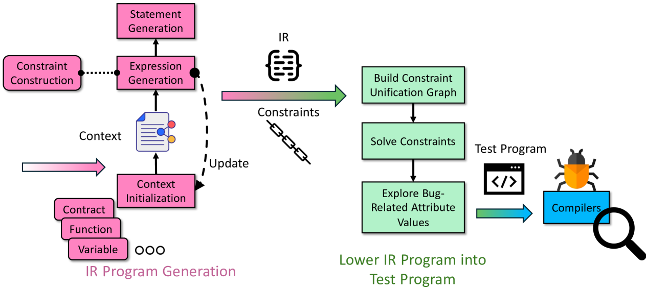
Figure 2. Erwin’s workflow

The workflow of Erwin is depicted in Figure˜2. The process starts with the creation of an intermediate representation (IR) program to represent the program template, which is subsequently filled into a test program for compiler testing. The generation of the IR program starts with the initialization of a context, which serves to store declaration information such as scopes. Once the context is established, Erwin proceeds to generate expressions inside each suitable scope based on the declarations contained in the context. If no appropriate declarations are found in a scope, Erwin can also trigger updates to the context. Finally, Erwin assembles statements from the generated expressions (e.g., function call statements) and generates statements (e.g., return statements) in the suitable position to construct a complete program. The generated IR program contains attribute variables related to features such as data types, storage locations, visibility, and mutability. These attribute variables serve as the placeholders within the template. These are language features that have been found to be commonly associated with Solidity compiler bugs (Ma et al., 2024). These attribute variables require initialization with concrete attribute values during the IR lowering process. Since these attribute variables are propagated through expressions, Erwin constructs constraints to narrow down their value codomains or build relationships among them. We delve into the details of the IR program generation in section˜3.2. After the IR program is generated, Erwin proceeds to lower it into test programs, as described in section˜3.3. This process involves solving the constraints associated with the attribute variables to ensure that the generated IR program is correctly annotated with these attributes. The constraints are solved by constructing a constraint unification graph, which is used to determine the appropriate values for the attributes. Finally, the generated test programs can be compiled or analyzed by the compiler or analyzer to verify their correctness.

3.1. Preliminary Definitions

$$\langle p\in Program\rangle::= \overline{d}$$

$$\langle d\in Decl\rangle::= {\color[rgb]{1,.5,0}\mathfrak{A}}\ v\ |\ \mathsf{error}\ v(\overline{{\color[rgb]{1,.5,0}\mathfrak{A}}\ v\ })\ |\ \mathsf{event}\ v(\overline{{\color[rgb]{1,.5,0}\mathfrak{A}}\ v\ })\ |\ \mathsf{struct}\{\overline{{\color[rgb]{1,.5,0}\mathfrak{A}}\ v}\}\ |\ \mathsf{modifier}\ v(\overline{{\color[rgb]{1,.5,0}\mathfrak{A}}\ v\ })\{\overline{s}\}\$$

$$|\ \mathsf{function}\ (\overline{{\color[rgb]{1,.5,0}\mathfrak{A}}\ v\ })\ {\color[rgb]{1,.5,0}\mathfrak{A}}\ \{\overline{s}\}$$

$$\langle s\in Stmt\rangle::= e\ |\ {\color[rgb]{1,.5,0}\mathfrak{A}}\ v=e|\ \mathsf{if}\ (e)\ \{\overline{s}\}\ \mathsf{else}\ \{\overline{s}\}\ |\ \mathsf{for}\ (e;e;e)\ \{\overline{s}\}$$

$$|\ \mathsf{do}\ \{\overline{s}\}\ \mathsf{while}\ (e)\ |\ \mathsf{while}\ (e)\ \{\overline{s}\}\ |\ \mathsf{return}\ e\ |\ \mathsf{emit}\ e\ |\ \mathsf{revert}\ e$$

$$\langle e\in Exp\rangle::= \text{literal}\ |\ v\ |\ v\ \mathit{op}_{a}\ e\ |\ e\ \mathit{op}_{b}\ e\ |\ \mathit{op}_{u}\ e\ |\ \mathsf{new}\ v\ |\ e\ ?\ e\ :\ e|\ v(\overline{e})\ |\ e[e]\ |\ e.v$$

$${\color[rgb]{1,.5,0}\mathfrak{A}}::= \text{a sequence of attribute variables, each of which is denoted as }{\color[rgb]{1,0,0}\mathscr{A}}$$

$$v::=$$ an identifier representing the name of a variable, method or contract

$$\mathit{op}_{a},\ \mathit{op}_{b},\ \mathit{op}_{u}::=$$ identifiers representing assignment, binary, unary operators

Figure 3. Syntax of IR, Where $\overline{x}$ Denotes a Sequence of $x$ Elements

The syntax of our IR is illustrated in Figure˜3, with certain elements like abstract contracts, interfaces, type aliases, and enums omitted for simplicity. Additionally, inline assembly, which pertains to a different language domain, is not included in this formalization. As of this writing, Erwin does not support these features yet, but we plan to extend support for them in the future. A variable or method can be qualified by a sequence of attribute variables, each of which can take on an attribute value that act as the qualifier for the variable or the method during the IR lowering process (section˜3.3). Specifically tailored for Solidity, an attribute variable ${\color[rgb]{1,0,0}\mathscr{A}}$ can be ${\color[rgb]{1,0,0}\mathscr{T}}$, ${\color[rgb]{1,0,0}\mathscr{S}}$, ${\color[rgb]{1,0,0}\mathscr{V}}$, and ${\color[rgb]{1,0,0}\mathscr{M}}$, each of which represents the attribute variable for data type, storage location, visibility, and mutability, respectively. The collection of attribute values that can be assigned to an attribute variable is referred to as the attribute value codomain, symbolized by ${\color[rgb]{.75,.5,.25}\tau}$. Figure˜4 lists the initial attribute value codomain of each kind attribute variable.

$${\color[rgb]{.75,.5,.25}\tau}_{{\color[rgb]{1,0,0}\mathscr{T}}}::=\ \{ \mathsf{bool},\ \mathsf{address},\ \mathsf{address\ payable},\ \mathsf{string},\ \mathsf{(u)int}_{x}\ ,\ x\in\{\epsilon,8,16,32,64,128,256\},$$

$$\text{struct type},\ \text{contract type},\ \text{array type},\ \text{mapping type}\}$$

$${\color[rgb]{.75,.5,.25}\tau}_{{\color[rgb]{1,0,0}\mathscr{S}}}::=\ \{ \mathsf{memory},\ \mathsf{storage}\text{ pointer},\ \mathsf{storage}\text{ reference},\ \mathsf{calldata}\}$$

$${\color[rgb]{.75,.5,.25}\tau}_{{\color[rgb]{1,0,0}\mathscr{V}}}::=\ \{ \mathsf{public},\ \mathsf{private},\ \mathsf{internal},\ \mathsf{external}\}$$

$${\color[rgb]{.75,.5,.25}\tau}_{{\color[rgb]{1,0,0}\mathscr{M}}}::=\ \{ \mathsf{pure},\ \mathsf{view},\ \mathsf{payable},\ \mathsf{nonpayable}\}$$

Figure 4. Attribute Value Codomain Initialization in Solidity

While the IR of Figure˜3 has been designed for Solidity, it can be easily adapted or extended for other programming languages. For instance, the kinds of attribute variables can be expanded or reduced to suit the target langauge. Additionally, declarations, statements, and expressions can be customized by adding, removing, or substituting elements to better align the IR with the target language. For instance, Solidity’s modifier declaration could be replaced with Python’s decorator declaration, and the concept of a contract in Solidity can be adapted to correspond to a class in other object-oriented programming languages.

3.2. IR Program Generation

Context Initialization.  Erwin’s generation approach is hierarchical, starting with the creation of contract declarations. This is followed by the declarations of contract members, such as member variables and member functions, as well as parameter declarations, and so forth. These declarations, along with their scopes and associated attribute variables, define the context of the program. Formally, the context $\Gamma$ begins empty and is equipped with the following helper functions.

• $\Gamma.\texttt{push}(d,s,{\color[rgb]{1,0,0}\mathscr{A}}_{d})$: generate a declaration $d$ in scope $s$, associate it with attribute variable ${\color[rgb]{1,0,0}\mathscr{A}}_{d}$, and push them into $\Gamma$. If $s$ is qualified by more than one attribute variable, push all tuples into $\Gamma$.

• $\Gamma.\texttt{query}(s)$: obtain all $(d,{\color[rgb]{1,0,0}\mathscr{A}}_{d})$ pair from scope $s$ and all scopes that are visible to $s$.

• $\Gamma.\texttt{scope}(d)$: returns the scope of declaration $d$.

• $\Gamma.\texttt{findVisibleScopes}(s)$: returns a set of scopes that are visible from the scope $s$.

During the context initialization phase, Erwin systematically applies $\Gamma.\texttt{push}$ operations to scaffold the architectural blueprint of relevant smart contracts. This includes declaring core components (contract templates, function signatures, variable declarations) while deferring concrete implementation details to later phases, in which these skeletal structures will be filled with expressions and statements.

Expression Generation and Constraint Construction.  The expression generation is carried out in a top-down manner. Specifically, if Erwin intends to generate an expression $e$ from $\Gamma$, it first analyzes the necessary sub-expressions $\overline{e_{s}}$ and gathers the required constraints among $e$’s attribute variables and those of $\overline{e_{s}}$. Subsequently, Erwin generates $\overline{e_{s}}$ based on the constraints. Finally, Erwin collects all the associated constraints in the generation of $e$ and pushes them into the attribute constraint set ${\color[rgb]{.5,0,.5}\mathbb{C}}$.

Definition 3.1 (Attribute Constraint Set).

An attribute constraint set ${\color[rgb]{.5,0,.5}\mathbb{C}}$ comprises:

• A collection of relations $\{{\color[rgb]{1,0,0}\mathscr{A}}_{i}\bowtie{\color[rgb]{1,0,0}\mathscr{A}}_{j}\}$, where ${\color[rgb]{1,0,0}\mathscr{A}}_{i}$ and ${\color[rgb]{1,0,0}\mathscr{A}}_{j}$ are attribute variables and
  $\bowtie\ \in\{\doteq,\ \lessdot\}$. Here, $\doteq$ and $\lessdot$ signify “is the same as" and “is more restricted than”, respectively.

• A collection of codomain restriction of attribute variables such as ${\color[rgb]{.75,.5,.25}\tau}_{{\color[rgb]{1,0,0}\mathscr{A}}}\leftarrow\{\ldots\}$ or $A_{i}\lessdot{\color[rgb]{1,0,0}\mathscr{A}}\lessdot A_{j}$ where $A_{i}$ and $A_{j}$ are attribute values. The first restriction assigns a new codomain to ${\color[rgb]{.75,.5,.25}\tau}_{{\color[rgb]{1,0,0}\mathscr{A}}}$ where the second sets the upper bound and lower bound of ${\color[rgb]{.75,.5,.25}\tau}_{{\color[rgb]{1,0,0}\mathscr{A}}}$. This kind of constraint directly modifies the codomain of an attribute variable.

In a constraint ${\color[rgb]{1,0,0}\mathscr{A}}_{i}\bowtie{\color[rgb]{1,0,0}\mathscr{A}}_{j}$, the attribute variables must represent attributes of the same kind (e.g. it is meaningless to impose a constraint between, say, a data type and a storage location).

Like the traditional subtyping relation, $\lessdot$ is both reflexive and transitive. It conveys different meanings across attribute kinds:

• Data types: ${\color[rgb]{1,0,0}\mathscr{T}}_{1}\lessdot{\color[rgb]{1,0,0}\mathscr{T}}_{2}$ means that ${\color[rgb]{1,0,0}\mathscr{T}}_{1}$ is a subtype of ${\color[rgb]{1,0,0}\mathscr{T}}_{2}$, e.g., $\mathsf{int}_{16}\lessdot\mathsf{int}_{32}$.

• Storage locations: ${\color[rgb]{1,0,0}\mathscr{S}}_{1}\lessdot{\color[rgb]{1,0,0}\mathscr{S}}_{2}$ means that data stored in ${\color[rgb]{1,0,0}\mathscr{S}}_{1}$ can be transferred to ${\color[rgb]{1,0,0}\mathscr{S}}_{2}$, e.g., $\mathsf{calldata}\lessdot\mathsf{memory}$.

• Visibilities (${\color[rgb]{1,0,0}\mathscr{V}})$ and mutabilities (${\color[rgb]{1,0,0}\mathscr{M}}$) are not governed by relations.

The constraint set ${\color[rgb]{.5,0,.5}\mathbb{C}}$ is initialized by propagating the initial codomains of all kinds of attribute variables (as defined in Figure˜4) to their respective instances after context initialization. The scope can refine ${\color[rgb]{.75,.5,.25}\tau}_{{\color[rgb]{1,0,0}\mathscr{S}}_{i}}$ during constraint set initialization. For example, ${\color[rgb]{.75,.5,.25}\tau}_{{\color[rgb]{1,0,0}\mathscr{S}}_{i}}::=\{\mathsf{storage}\text{ reference}\}$ if ${\color[rgb]{1,0,0}\mathscr{S}}_{i}$ resides in a contract’s member scope. Such language-specific refinements are intentionally excluded from formalization to preserve simplicity and readability.

We formalize the process of generating expressions and constructing constraints independently for every participating attribute variable. To structure this formally, we define $\texttt{GEN}^{s}_{{\color[rgb]{.5,0,.5}\mathbb{C}}}(e:{\color[rgb]{1,0,0}\mathscr{A}}_{e})$ as the generative procedure for expression $e$ in scope $s$ under constraints related to a newly defined ${\color[rgb]{1,0,0}\mathscr{A}}_{e}$ in the constraint set ${\color[rgb]{.5,0,.5}\mathbb{C}}$ while pushing the initialization of ${\color[rgb]{.75,.5,.25}\tau}_{{\color[rgb]{1,0,0}\mathscr{A}}_{e}}$ to ${\color[rgb]{.5,0,.5}\mathbb{C}}$, and fraction line as the operator for breaking down a generation process.

(1) $$\scriptsize\frac{\texttt{GEN}^{s}_{{\color[rgb]{.5,0,.5}\mathbb{C}}}(e)}{\texttt{GEN}^{s}_{{\color[rgb]{.5,0,.5}\mathbb{C}}.\texttt{push}(\mathit{constraints\ for}\ {\color[rgb]{1,0,0}\mathscr{A}}_{e_{1}})}(e_{1}:{\color[rgb]{1,0,0}\mathscr{A}}_{e_{1}})\quad\texttt{GEN}^{s}_{{\color[rgb]{.5,0,.5}\mathbb{C}}.\texttt{push}(\mathit{constraints\ for}\ {\color[rgb]{1,0,0}\mathscr{A}}_{e_{2}})}(e_{2}:{\color[rgb]{1,0,0}\mathscr{A}}_{e_{2}})\quad\ldots}$$

For instance, eq.˜1 expresses that generating $e$ involves decomposing it into the generation of all its constituent subexpressions $e_{1},e_{2},\ldots$. In the demonstrated formula, ${\color[rgb]{.5,0,.5}\mathbb{C}}.\texttt{push}$ serves to incrementally update the global constraint set ${\color[rgb]{.5,0,.5}\mathbb{C}}$. Subexpressions are generated sequentially, ensuring constraints derived for $e_{1}$ become visible to the subsequent generator of $e_{2}$, as shown in the example.

$$\frac{}{\texttt{GEN}^{s}_{{\color[rgb]{.5,0,.5}\mathbb{C}}.\texttt{push}(\texttt{LOWER\_BOUND}(l)\lessdot{\color[rgb]{1,0,0}\mathscr{T}}\lessdot\texttt{UPPER\_BOUND}(l))}(l:{\color[rgb]{1,0,0}\mathscr{T}})}\ \boxed{{\color[rgb]{1,0,0}\mathscr{T}}\text{-Lit}}\quad\frac{}{\texttt{GEN}^{s}_{{\color[rgb]{.5,0,.5}\mathbb{C}}.\texttt{push}({\color[rgb]{.75,.5,.25}\tau}_{{\color[rgb]{1,0,0}\mathscr{T}}}\leftarrow\{\texttt{typeof}(v)\})}(\mathsf{new}\ v:{\color[rgb]{1,0,0}\mathscr{T}})}\ \boxed{{\color[rgb]{1,0,0}\mathscr{T}}\text{-New}}$$

$$\frac{\begin{aligned} &(v,{\color[rgb]{1,0,0}\mathscr{T}}_{v})\in\Gamma.\texttt{query}(s)\\ &{\color[rgb]{.5,0,.5}\mathbb{C}}\cup\{{\color[rgb]{1,0,0}\mathscr{T}}\doteq{\color[rgb]{1,0,0}\mathscr{T}}_{v}\}\text{ is solvable}\end{aligned}}{\texttt{GEN}^{s}_{{\color[rgb]{.5,0,.5}\mathbb{C}}.\texttt{push}({\color[rgb]{1,0,0}\mathscr{T}}\doteq{\color[rgb]{1,0,0}\mathscr{T}}_{v})}(v:{\color[rgb]{1,0,0}\mathscr{T}})}\ \boxed{{\color[rgb]{1,0,0}\mathscr{T}}\text{-Ident}}\quad\frac{\texttt{GEN}^{s}_{{\color[rgb]{.5,0,.5}\mathbb{C}}}(v\ =\ e:{\color[rgb]{1,0,0}\mathscr{T}})}{\texttt{GEN}^{s}_{{\color[rgb]{.5,0,.5}\mathbb{C}}.\texttt{push}({\color[rgb]{1,0,0}\mathscr{T}}\doteq{\color[rgb]{1,0,0}\mathscr{T}}_{v})}(v:{\color[rgb]{1,0,0}\mathscr{T}}_{v})\quad\texttt{GEN}^{s}_{{\color[rgb]{.5,0,.5}\mathbb{C}}.\texttt{push}({\color[rgb]{1,0,0}\mathscr{T}}_{e}\lessdot{\color[rgb]{1,0,0}\mathscr{T}})}(e:{\color[rgb]{1,0,0}\mathscr{T}}_{e})}\ \boxed{{\color[rgb]{1,0,0}\mathscr{T}}\text{-Assi}_{1}}$$

$$\frac{\mathit{op}_{a}\in\{\mathrel{+}\mspace{-0.5mu}=,\mathrel{-}\mspace{-0.5mu}=,\mathrel{*}\mspace{-0.5mu}=,\mathrel{/}\mspace{-0.5mu}=,\mathrel{\%}\mkern-0.5mu=,\mathrel{\&}\mkern-0.5mu=,\mathrel{\textasciicircum}\mkern-0.4mu=,\mathrel{|}\mspace{-0.5mu}=\}\quad\texttt{GEN}^{s}_{{\color[rgb]{.5,0,.5}\mathbb{C}}.\texttt{push}(\mathsf{int}_{8}\lessdot{\color[rgb]{1,0,0}\mathscr{T}}\lessdot\mathsf{int}_{256}\ ||\ \mathsf{uint}_{8}\lessdot{\color[rgb]{1,0,0}\mathscr{T}}\lessdot\mathsf{uint}_{256})}(v\ \mathit{op}_{a}\ e:{\color[rgb]{1,0,0}\mathscr{T}})}{\texttt{GEN}^{s}_{{\color[rgb]{.5,0,.5}\mathbb{C}}.\texttt{push}({\color[rgb]{1,0,0}\mathscr{T}}\doteq{\color[rgb]{1,0,0}\mathscr{T}}_{v})}(v:{\color[rgb]{1,0,0}\mathscr{T}}_{v})\quad\texttt{GEN}^{s}_{{\color[rgb]{.5,0,.5}\mathbb{C}}.\texttt{push}({\color[rgb]{1,0,0}\mathscr{T}}_{e}\lessdot{\color[rgb]{1,0,0}\mathscr{T}})}(e:{\color[rgb]{1,0,0}\mathscr{T}}_{e})}\ \boxed{{\color[rgb]{1,0,0}\mathscr{T}}\text{-Assi}_{2}}$$

$$\frac{\mathit{op}_{a}\in\{{\mathrel{<\!\mkern-3.0mu<\!=}},{\mathrel{>\!\mkern-3.0mu>\!=}}\}\quad\texttt{GEN}^{s}_{{\color[rgb]{.5,0,.5}\mathbb{C}}.\texttt{push}(\mathsf{int}_{8}\lessdot{\color[rgb]{1,0,0}\mathscr{T}}\lessdot\mathsf{int}_{256}\ ||\ \mathsf{uint}_{8}\lessdot{\color[rgb]{1,0,0}\mathscr{T}}\lessdot\mathsf{uint}_{256})}(v\ \mathit{op}_{a}\ e:{\color[rgb]{1,0,0}\mathscr{T}})}{\texttt{GEN}^{s}_{{\color[rgb]{.5,0,.5}\mathbb{C}}.\texttt{push}({\color[rgb]{1,0,0}\mathscr{T}}\doteq{\color[rgb]{1,0,0}\mathscr{T}}_{v})}(v:{\color[rgb]{1,0,0}\mathscr{T}}_{v})\quad\texttt{GEN}^{s}_{{\color[rgb]{.5,0,.5}\mathbb{C}}.\texttt{push}(\mathsf{uint}_{8}\lessdot{\color[rgb]{1,0,0}\mathscr{T}}_{e}\lessdot\mathsf{uint}_{256})}(e:{\color[rgb]{1,0,0}\mathscr{T}}_{e})}\ \boxed{{\color[rgb]{1,0,0}\mathscr{T}}\text{-Assi}_{3}}$$

$$\frac{\texttt{GEN}^{s}_{{\color[rgb]{.5,0,.5}\mathbb{C}}.\texttt{push}({\color[rgb]{.75,.5,.25}\tau}_{{\color[rgb]{1,0,0}\mathscr{T}}}\leftarrow\{\mathsf{bool}\})}(!\ e:{\color[rgb]{1,0,0}\mathscr{T}})}{\texttt{GEN}^{s}_{{\color[rgb]{.5,0,.5}\mathbb{C}}.\texttt{push}({\color[rgb]{1,0,0}\mathscr{T}}_{e}\doteq{\color[rgb]{1,0,0}\mathscr{T}})}(e:{\color[rgb]{1,0,0}\mathscr{T}}_{e})}\ \boxed{{\color[rgb]{1,0,0}\mathscr{T}}\text{-Uop}_{1}}\quad\frac{\texttt{GEN}^{s}_{{\color[rgb]{.5,0,.5}\mathbb{C}}.\texttt{push}(\mathsf{int}_{8}\lessdot{\color[rgb]{1,0,0}\mathscr{T}}\lessdot\mathsf{int}_{256})}(-\ e:{\color[rgb]{1,0,0}\mathscr{T}})}{\texttt{GEN}^{s}_{{\color[rgb]{.5,0,.5}\mathbb{C}}.\texttt{push}({\color[rgb]{1,0,0}\mathscr{T}}_{e}\doteq{\color[rgb]{1,0,0}\mathscr{T}})}(e:{\color[rgb]{1,0,0}\mathscr{T}}_{e})}\ \boxed{{\color[rgb]{1,0,0}\mathscr{T}}\text{-Uop}_{2}}$$

$$\frac{\mathit{op}_{u}\in\{\sim,\mathit{++},\mathit{--}\}\quad\texttt{GEN}^{s}_{{\color[rgb]{.5,0,.5}\mathbb{C}}.\texttt{push}(\mathsf{int}_{8}\lessdot{\color[rgb]{1,0,0}\mathscr{T}}\lessdot\mathsf{int}_{256}\ ||\ \mathsf{uint}_{8}\lessdot{\color[rgb]{1,0,0}\mathscr{T}}\lessdot\mathsf{uint}_{256})}(\mathit{op}_{u}\ e:{\color[rgb]{1,0,0}\mathscr{T}})}{\texttt{GEN}^{s}_{{\color[rgb]{.5,0,.5}\mathbb{C}}.\texttt{push}({\color[rgb]{1,0,0}\mathscr{T}}_{e}\doteq{\color[rgb]{1,0,0}\mathscr{T}})}(e:{\color[rgb]{1,0,0}\mathscr{T}}_{e})}\ \boxed{{\color[rgb]{1,0,0}\mathscr{T}}\text{-Uop}_{3}}$$

$$\frac{\mathit{op}_{b}\in\{>,<,\leq,\geq,\mathrel{=}\mspace{-0.5mu}=,\neq\}\quad\texttt{GEN}^{s}_{{\color[rgb]{.5,0,.5}\mathbb{C}}.\texttt{push}({\color[rgb]{.75,.5,.25}\tau}_{{\color[rgb]{1,0,0}\mathscr{T}}}\leftarrow\{\mathsf{bool}\})}(e_{1}\ \mathit{op}_{b}\ e_{2}:{\color[rgb]{1,0,0}\mathscr{T}})}{\texttt{GEN}^{s}_{{\color[rgb]{.5,0,.5}\mathbb{C}}.\texttt{push}(\mathsf{int}_{8}\lessdot{\color[rgb]{1,0,0}\mathscr{T}}_{e_{1}}\lessdot\mathsf{int}_{256}\ ||\ \mathsf{uint}_{8}\lessdot{\color[rgb]{1,0,0}\mathscr{T}}_{e_{1}}\lessdot\mathsf{uint}_{256})}(e_{1}:{\color[rgb]{1,0,0}\mathscr{T}}_{e_{1}})\quad\texttt{GEN}^{s}_{{\color[rgb]{.5,0,.5}\mathbb{C}}.\texttt{push}({\color[rgb]{1,0,0}\mathscr{T}}_{e_{1}}\lessdot{\color[rgb]{1,0,0}\mathscr{T}}_{e_{2}}\ ||\ {\color[rgb]{1,0,0}\mathscr{T}}_{e_{2}}\lessdot{\color[rgb]{1,0,0}\mathscr{T}}_{e_{1}})}(e_{2}:{\color[rgb]{1,0,0}\mathscr{T}}_{e_{2}})}\ \boxed{{\color[rgb]{1,0,0}\mathscr{T}}\text{-Bop}_{1}}$$

$$\frac{\mathit{op}_{b}\in\{+,-,*,/,\%,\&\,\textasciicircum,|\}\quad\texttt{GEN}^{s}_{{\color[rgb]{.5,0,.5}\mathbb{C}}.\texttt{push}(\mathsf{int}_{8}\lessdot{\color[rgb]{1,0,0}\mathscr{T}}_{e}\lessdot\mathsf{int}_{256}\ ||\ \mathsf{uint}_{8}\lessdot{\color[rgb]{1,0,0}\mathscr{T}}_{e}\lessdot\mathsf{uint}_{256})}(e_{1}\ \mathit{op}_{b}\ e_{2}:{\color[rgb]{1,0,0}\mathscr{T}})}{\texttt{GEN}^{s}_{{\color[rgb]{.5,0,.5}\mathbb{C}}.\texttt{push}({\color[rgb]{1,0,0}\mathscr{T}}_{e_{1}}\lessdot{\color[rgb]{1,0,0}\mathscr{T}})}(e_{1}:{\color[rgb]{1,0,0}\mathscr{T}}_{e_{1}})\quad\texttt{GEN}^{s}_{{\color[rgb]{.5,0,.5}\mathbb{C}}.\texttt{push}({\color[rgb]{1,0,0}\mathscr{T}}_{e_{2}}\lessdot{\color[rgb]{1,0,0}\mathscr{T}})}(e_{2}:{\color[rgb]{1,0,0}\mathscr{T}}_{e_{2}})}\ \boxed{{\color[rgb]{1,0,0}\mathscr{T}}\text{-Bop}_{2}}$$

$$\frac{\mathit{op}_{b}\in\{{\mathrel{<\!\mkern-3.0mu<\!}},{\mathrel{>\!\mkern-3.0mu>\!}}\}\quad\texttt{GEN}^{s}_{{\color[rgb]{.5,0,.5}\mathbb{C}}.\texttt{push}(\mathsf{int}_{8}\lessdot{\color[rgb]{1,0,0}\mathscr{T}}\lessdot\mathsf{int}_{256}\ ||\ \mathsf{uint}_{8}\lessdot{\color[rgb]{1,0,0}\mathscr{T}}\lessdot\mathsf{uint}_{256})}(e_{1}\ \mathit{op}_{b}\ e_{2}:{\color[rgb]{1,0,0}\mathscr{T}})}{\texttt{GEN}^{s}_{{\color[rgb]{.5,0,.5}\mathbb{C}}.\texttt{push}({\color[rgb]{1,0,0}\mathscr{T}}_{e_{1}}\lessdot{\color[rgb]{1,0,0}\mathscr{T}})}(e_{1}:{\color[rgb]{1,0,0}\mathscr{T}}_{e_{1}})\quad\texttt{GEN}^{s}_{{\color[rgb]{.5,0,.5}\mathbb{C}}.\texttt{push}(\mathsf{uint}_{8}\lessdot{\color[rgb]{1,0,0}\mathscr{T}}_{e_{2}}\lessdot\mathsf{uint}_{256})}(e_{2}:{\color[rgb]{1,0,0}\mathscr{T}}_{e_{2}})}\ \boxed{{\color[rgb]{1,0,0}\mathscr{T}}\text{-Bop}_{3}}$$

$$\frac{\mathit{op}_{b}\in\{\&\&,||\}\quad\texttt{GEN}^{s}_{{\color[rgb]{.5,0,.5}\mathbb{C}}.\texttt{push}({\color[rgb]{.75,.5,.25}\tau}_{{\color[rgb]{1,0,0}\mathscr{T}}}\leftarrow\{\mathsf{bool}\})}(e_{1}\ \mathit{op}_{b}\ e_{2}:{\color[rgb]{1,0,0}\mathscr{T}})}{\texttt{GEN}^{s}_{{\color[rgb]{.5,0,.5}\mathbb{C}}.\texttt{push}({\color[rgb]{1,0,0}\mathscr{T}}_{e_{1}}\lessdot{\color[rgb]{1,0,0}\mathscr{T}})}(e_{1}:{\color[rgb]{1,0,0}\mathscr{T}}_{e_{1}})\quad\texttt{GEN}^{s}_{{\color[rgb]{.5,0,.5}\mathbb{C}}.\texttt{push}({\color[rgb]{1,0,0}\mathscr{T}}_{e_{2}}\lessdot{\color[rgb]{1,0,0}\mathscr{T}})}(e_{2}:{\color[rgb]{1,0,0}\mathscr{T}}_{e_{2}})}\ \boxed{{\color[rgb]{1,0,0}\mathscr{T}}\text{-Bop}_{4}}$$

$$\frac{\texttt{GEN}^{s}_{{\color[rgb]{.5,0,.5}\mathbb{C}}}(e_{1}\ ?\ e_{2}\ :\ e_{3}:{\color[rgb]{1,0,0}\mathscr{T}})}{\texttt{GEN}^{s}_{{\color[rgb]{.5,0,.5}\mathbb{C}}.\texttt{push}({\color[rgb]{.75,.5,.25}\tau}_{{\color[rgb]{1,0,0}\mathscr{T}}_{e_{1}}}\leftarrow\{\mathsf{bool}\})}(e_{1}:{\color[rgb]{1,0,0}\mathscr{T}}_{e_{1}})\quad\texttt{GEN}^{s}_{{\color[rgb]{.5,0,.5}\mathbb{C}}.\texttt{push}({\color[rgb]{1,0,0}\mathscr{T}}_{e_{2}}\lessdot{\color[rgb]{1,0,0}\mathscr{T}})}(e_{2}:{\color[rgb]{1,0,0}\mathscr{T}}_{e_{2}})\quad\texttt{GEN}^{s}_{{\color[rgb]{.5,0,.5}\mathbb{C}}.\texttt{push}({\color[rgb]{1,0,0}\mathscr{T}}_{e_{3}}\lessdot{\color[rgb]{1,0,0}\mathscr{T}})}(e_{3}:{\color[rgb]{1,0,0}\mathscr{T}}_{e_{3}})}\ \boxed{{\color[rgb]{1,0,0}\mathscr{T}}\text{-Cond}}$$

$$\frac{(f,({\color[rgb]{1,0,0}\mathscr{T}}_{1},{\color[rgb]{1,0,0}\mathscr{T}}_{2},\ldots)\rightarrow{\color[rgb]{1,0,0}\mathscr{T}}_{f})\in\Gamma.\texttt{query}(s)\quad\texttt{GEN}^{s}_{{\color[rgb]{.5,0,.5}\mathbb{C}}.\texttt{push}({\color[rgb]{1,0,0}\mathscr{T}}\doteq{\color[rgb]{1,0,0}\mathscr{T}}_{f})}(f(e_{1},e_{2},\ldots):{\color[rgb]{1,0,0}\mathscr{T}})}{\texttt{GEN}^{s}_{{\color[rgb]{.5,0,.5}\mathbb{C}}.\texttt{push}({\color[rgb]{1,0,0}\mathscr{T}}_{e_{1}}\lessdot{\color[rgb]{1,0,0}\mathscr{T}}_{1})}(e_{1}:{\color[rgb]{1,0,0}\mathscr{T}}_{e_{1}})\quad\texttt{GEN}^{s}_{{\color[rgb]{.5,0,.5}\mathbb{C}}.\texttt{push}({\color[rgb]{1,0,0}\mathscr{T}}_{e_{2}}\lessdot{\color[rgb]{1,0,0}\mathscr{T}}_{2})}(e_{2}:{\color[rgb]{1,0,0}\mathscr{T}}_{e_{2}})\quad\ldots}\ \boxed{{\color[rgb]{1,0,0}\mathscr{T}}\text{-Apply}}$$

$$\frac{\texttt{GEN}^{s}_{{\color[rgb]{.5,0,.5}\mathbb{C}}}(e_{1}[e_{2}]:{\color[rgb]{1,0,0}\mathscr{T}})}{\texttt{GEN}^{s}_{{\color[rgb]{.5,0,.5}\mathbb{C}}.\texttt{push}(\mathsf{uint}_{8}\lessdot{\color[rgb]{1,0,0}\mathscr{T}}_{e_{2}}\lessdot\mathsf{uint}_{256})}(e_{2}:{\color[rgb]{1,0,0}\mathscr{T}}_{e_{2}})\quad\texttt{GEN}^{s}_{{\color[rgb]{.5,0,.5}\mathbb{C}}.\texttt{push}({\color[rgb]{1,0,0}\mathscr{T}}_{e_{1}}.\texttt{base}\doteq{\color[rgb]{1,0,0}\mathscr{T}})}(e_{1}:{\color[rgb]{1,0,0}\mathscr{T}}_{e_{1}})}\ \boxed{{\color[rgb]{1,0,0}\mathscr{T}}\text{-Ind}}$$

Figure 5. Constraint Rules for Data Type

Figure˜5 describes the expression generation procedure under constraints for data types. These rules are designed to model the relationships between data type variables and their interactions with operators and expressions. For instance, The ${\color[rgb]{1,0,0}\mathscr{T}}\text{-Lit}$ construct illustrates that generating a literal $l$ enforces type constraints on ${\color[rgb]{1,0,0}\mathscr{T}}_{l}$, where these constraints bound ${\color[rgb]{1,0,0}\mathscr{T}}_{l}$ between LOWER_BOUND, the bottom data type for $l$, and UPPER_BOUND, the top data type for $l$. The ${\color[rgb]{1,0,0}\mathscr{T}}\text{-Ident}$ construct specifies that identifiers such as $v$ or $e.v$ are generated from previously declared variables, without imposing additional type constraints. The ${\color[rgb]{1,0,0}\mathscr{T}}\text{-New}$ construct specifies that in a new expression, the codomain of its data type variable ${\color[rgb]{1,0,0}\mathscr{T}}$ is constrained by the user-defined type implied in the new expression, i.e., $\texttt{typeof}(v)$. For instance, if the new expression is $\texttt{new}\ C$ where $C$ is a contract name, then the codomain of ${\color[rgb]{1,0,0}\mathscr{T}}$ is restricted to $\texttt{typeof}(C)$, which is a contract type. The choice of assignment operators can impose different constraints. For example, in an assignment expression $v\ \mathit{op}_{a}\ e:{\color[rgb]{1,0,0}\mathscr{T}}$, the $=$ operator introduces no constraints on ${\color[rgb]{1,0,0}\mathscr{T}}$ (${\color[rgb]{1,0,0}\mathscr{T}}\text{-Assi}_{1}$), while other assignment operators enforce $\mathsf{int}_{8}\lessdot{\color[rgb]{1,0,0}\mathscr{T}}\lessdot\mathsf{int}_{256}$ or $\mathsf{uint}_{8}\lessdot{\color[rgb]{1,0,0}\mathscr{T}}\lessdot\mathsf{uint}_{256}$ (${\color[rgb]{1,0,0}\mathscr{T}}\text{-Assi}_{2}$ and ${\color[rgb]{1,0,0}\mathscr{T}}\text{-Assi}_{3}$). Binary and unary operations similarly impose operator-dependent constraints. The ${\color[rgb]{1,0,0}\mathscr{T}}\text{-Cond}$ rule governs conditional expressions $e_{1}\ ?\ e_{2}\ :\ e_{3}$, requiring $e_{1}$ to resolve to a boolean type and relating ${\color[rgb]{1,0,0}\mathscr{T}}_{e_{2}}$ and ${\color[rgb]{1,0,0}\mathscr{T}}_{e_{3}}$ to ${\color[rgb]{1,0,0}\mathscr{T}}$. The ${\color[rgb]{1,0,0}\mathscr{T}}\text{-Apply}$ rule activates for function calls and mapping uses, enforcing type compatibility between arguments and parameters through constraints $\{{\color[rgb]{1,0,0}\mathscr{T}}_{e_{i}}\lessdot{\color[rgb]{1,0,0}\mathscr{T}}_{i}\}$. ${\color[rgb]{1,0,0}\mathscr{T}}\text{-Ind}$ requires index accesses $e_{1}[e_{2}]$’s data type variable ${\color[rgb]{1,0,0}\mathscr{T}}$ inherits from array $e_{1}$’s base data type ${\color[rgb]{1,0,0}\mathscr{T}}_{e_{1}}.\texttt{base}$, with $e_{2}$ constrained to an unsigned integer type. ${\color[rgb]{1,0,0}\mathscr{T}}\text{-Ind}$ indicates that a data type variable (${\color[rgb]{1,0,0}\mathscr{T}}_{e_{1}}.\texttt{base}$) may be the composition of another one (${\color[rgb]{1,0,0}\mathscr{T}}_{e_{1}}$). This relation complicates the constraint set so that we remove all data type variables which have base variables by rewriting all related constraints in ${\color[rgb]{.5,0,.5}\mathbb{C}}$ with the following steps.

• Recursively propagate constraints between type variables to their bases, continuing this process until the bases no longer have any further bases.

• Rename ${\color[rgb]{1,0,0}\mathscr{T}}.\texttt{base}$ with a new data type variable ${\color[rgb]{1,0,0}\mathscr{T}}^{\prime}$.

• Remove all type variables containing bases.

$$\frac{}{\texttt{GEN}_{{\color[rgb]{.5,0,.5}\mathbb{C}}}^{s}(l:{\color[rgb]{1,0,0}\mathscr{S}})}\ \boxed{{\color[rgb]{1,0,0}\mathscr{S}}\text{-Lit}}\quad\frac{}{\texttt{GEN}_{{\color[rgb]{.5,0,.5}\mathbb{C}}}^{s}(\mathsf{new}\ v:{\color[rgb]{1,0,0}\mathscr{S}})}\ \boxed{{\color[rgb]{1,0,0}\mathscr{S}}\text{-New}}\quad\frac{(v,{\color[rgb]{1,0,0}\mathscr{S}}_{v})\in\Gamma.\texttt{query}(s)\quad{\color[rgb]{.5,0,.5}\mathbb{C}}\cup\{{\color[rgb]{1,0,0}\mathscr{S}}\lessdot{\color[rgb]{1,0,0}\mathscr{S}}_{v}\}\text{ is solvable}}{\texttt{GEN}_{{\color[rgb]{.5,0,.5}\mathbb{C}}.\texttt{push}({\color[rgb]{1,0,0}\mathscr{S}}\lessdot{\color[rgb]{1,0,0}\mathscr{S}}_{v})}^{s}(v:{\color[rgb]{1,0,0}\mathscr{S}})}\ \boxed{{\color[rgb]{1,0,0}\mathscr{S}}\text{-Ident}}$$

$$\frac{\texttt{GEN}^{s}_{{\color[rgb]{.5,0,.5}\mathbb{C}}}(v\ =\ e:{\color[rgb]{1,0,0}\mathscr{S}})}{\texttt{GEN}^{s}_{{\color[rgb]{.5,0,.5}\mathbb{C}}.\texttt{push}({\color[rgb]{1,0,0}\mathscr{S}}_{v}\doteq{\color[rgb]{1,0,0}\mathscr{S}})}(v:{\color[rgb]{1,0,0}\mathscr{S}}_{v})\quad\texttt{GEN}^{s}_{{\color[rgb]{.5,0,.5}\mathbb{C}}.\texttt{push}({\color[rgb]{1,0,0}\mathscr{S}}_{e}\lessdot{\color[rgb]{1,0,0}\mathscr{S}})}(e:{\color[rgb]{1,0,0}\mathscr{S}}_{e})}\ \boxed{{\color[rgb]{1,0,0}\mathscr{S}}\text{-Assi}}$$

$$\frac{\texttt{GEN}^{s}_{{\color[rgb]{.5,0,.5}\mathbb{C}}}(e_{1}\ ?\ e_{2}\ :\ e_{3}:{\color[rgb]{1,0,0}\mathscr{S}})}{\texttt{GEN}^{s}_{{\color[rgb]{.5,0,.5}\mathbb{C}}}(e_{1}:{\color[rgb]{1,0,0}\mathscr{S}}_{e_{1}})\quad\texttt{GEN}^{s}_{{\color[rgb]{.5,0,.5}\mathbb{C}}.\texttt{push}({\color[rgb]{1,0,0}\mathscr{S}}_{e_{2}}\lessdot{\color[rgb]{1,0,0}\mathscr{S}})}(e_{2}:{\color[rgb]{1,0,0}\mathscr{S}}_{e_{2}})\quad\texttt{GEN}^{s}_{{\color[rgb]{.5,0,.5}\mathbb{C}}.\texttt{push}({\color[rgb]{1,0,0}\mathscr{S}}_{e_{3}}\lessdot{\color[rgb]{1,0,0}\mathscr{S}})}(e_{3}:{\color[rgb]{1,0,0}\mathscr{S}}_{e_{3}})}\ \boxed{{\color[rgb]{1,0,0}\mathscr{S}}\text{-Cond}}$$

$$\frac{(f,({\color[rgb]{1,0,0}\mathscr{S}}_{1},{\color[rgb]{1,0,0}\mathscr{S}}_{2},\ldots)\rightarrow{\color[rgb]{1,0,0}\mathscr{S}}_{f})\in\Gamma.\texttt{query}(s)\quad\texttt{GEN}^{s}_{{\color[rgb]{.5,0,.5}\mathbb{C}}.\texttt{push}({\color[rgb]{1,0,0}\mathscr{S}}\doteq{\color[rgb]{1,0,0}\mathscr{S}}_{f})}(f(e_{1},e_{2},\ldots):{\color[rgb]{1,0,0}\mathscr{S}})}{\texttt{GEN}^{s}_{{\color[rgb]{.5,0,.5}\mathbb{C}}.\texttt{push}({\color[rgb]{1,0,0}\mathscr{S}}_{e_{1}}\lessdot{\color[rgb]{1,0,0}\mathscr{S}}_{1})}(e_{1}:{\color[rgb]{1,0,0}\mathscr{S}}_{e_{1}})\quad\texttt{GEN}^{s}_{{\color[rgb]{.5,0,.5}\mathbb{C}}.\texttt{push}({\color[rgb]{1,0,0}\mathscr{S}}_{e_{2}}\lessdot{\color[rgb]{1,0,0}\mathscr{S}}_{2})}(e_{2}:{\color[rgb]{1,0,0}\mathscr{S}}_{e_{2}})\quad\ldots}\ \boxed{{\color[rgb]{1,0,0}\mathscr{S}}\text{-Apply}}$$

Figure 6. Constraint Rules for Storage Location

The rules governing storage locations differ somewhat from those for data types. Notably, binary operations, unary operations, and index access operations are not applicable to storage locations. ${\color[rgb]{1,0,0}\mathscr{S}}\text{-Lit},{\color[rgb]{1,0,0}\mathscr{S}}\text{-New}$ do not introduce new constraints to ${\color[rgb]{.5,0,.5}\mathbb{C}}$. Assignment expressions are relevant when the operator is $=$. Other assignment operators, such as $\mathrel{+}\mspace{-0.5mu}=$ and $\mathrel{-}\mspace{-0.5mu}=$, are not included in this formalization since they only take effect on integers, which are not qualified by storage locations. The rules are summarized in Figure˜6. Once all storage location variable initializations and associated constraints are incorporated into ${\color[rgb]{.5,0,.5}\mathbb{C}}$, Erwin eliminates the storage location variables tied to expressions and declarations from ${\color[rgb]{.5,0,.5}\mathbb{C}}$ if the expressions or the declarations are associated with data type variables, such as ${\color[rgb]{1,0,0}\mathscr{T}}$. This occurs when ${\color[rgb]{.75,.5,.25}\tau}_{{\color[rgb]{1,0,0}\mathscr{T}}}\cap\{\mathsf{string},\text{mapping type},\text{struct type},\text{array type}\}\neq\emptyset$, as these specific data types in Solidity do not require qualification by storage locations.

Both ${\color[rgb]{1,0,0}\mathscr{T}}\text{-Ident}$ and ${\color[rgb]{1,0,0}\mathscr{S}}\text{-Ident}$ necessitate the presence of a declaration where the attribute variables meet the specified constraints. However, there are instances where this condition is not fulfilled. In these situations, Erwin calls context_update to insert a new declaration to $\Gamma$ if no suitable declaration exists.

Algorithm 1 Algorithm for Updating Context $\Gamma$

1:Inputs: The context $\Gamma$, the constraint set ${\color[rgb]{.5,0,.5}\mathbb{C}}$, the current scope $s$, the attribute variable ${\color[rgb]{1,0,0}\mathscr{A}}$ of the identifier.

2:procedure context_update($\Gamma$, ${\color[rgb]{.5,0,.5}\mathbb{C}}$, $s$, ${\color[rgb]{1,0,0}\mathscr{A}}$)

3:  $D$ is the set of declarations collected from $\Gamma.\texttt{query}(s)$.

4:  for $(d,{\color[rgb]{1,0,0}\mathscr{A}}_{d})\in\Gamma.\texttt{query}(s)$ do

5:   if $\Gamma.\texttt{scope}(d)\notin\Gamma.\texttt{findVisibleScopes}(s)$ then

6:     $\text{Remove}\ d\ \text{from}\ D$

7:   end if

8:   if ${\color[rgb]{.75,.5,.25}\tau}_{{\color[rgb]{1,0,0}\mathscr{A}}_{d}}\cap{\color[rgb]{.75,.5,.25}\tau}_{{\color[rgb]{1,0,0}\mathscr{A}}}=\emptyset$ then

9:     $\text{Remove}\ d\ \text{from}\ D$

10:   else

11:     ${\color[rgb]{.5,0,.5}\mathbb{C}}^{\prime}\leftarrow{\color[rgb]{.5,0,.5}\mathbb{C}}\bigcup\{{\color[rgb]{.75,.5,.25}\tau}_{{\color[rgb]{1,0,0}\mathscr{A}}_{d}}\leftarrow{\color[rgb]{.75,.5,.25}\tau}_{{\color[rgb]{1,0,0}\mathscr{A}}_{d}}\cap{\color[rgb]{.75,.5,.25}\tau}_{{\color[rgb]{1,0,0}\mathscr{A}}}\}$

12:     if ${\color[rgb]{.5,0,.5}\mathbb{C}}^{\prime}\ \text{is not solvable}$ then

13:      $\text{Remove}\ d\ \text{from}\ D$

14:     end if

15:   end if

16:  end for

17:  if $D=\emptyset$ then

18:   Pick $s_{d}$ randomly from $\Gamma.\texttt{findVisibleScopes}(s)$

19:   $\Gamma.\texttt{push}(d,s_{d},{\color[rgb]{1,0,0}\mathscr{A}}_{d})$

20:  end if

21:end procedure

Algorithm˜1 is called during the generation of identifier expressions to retrieve available declarations and update the context by adding new ones if no suitable declarations are found. The algorithm is divided into two primary steps: (1) checking for existing available declarations (lines 4-16), and (2) modifying the context by adding new declarations when none are available (lines 17-20). In the first step, Erwin filters out declarations that are out of scope (lines 5-7) and excludes those whose attribute value codomain does not overlap with the attribute variable codomain of the identifier (lines 8-10). Finally, if a declaration is selected as the origin of the identifier, Erwin attempts to modify the constraint set accordingly (line 11). However, if the updated constraint set becomes unsolvable, the update is reverted, and the declaration is excluded (lines 12-14). The process of determining solvability involves enumerating the possible values for each attribute from its codomain and verifying whether there are assignments of attribute values to each attribute variable that fulfill all the given relations. In the second step, if no suitable declaration is found (line 17), Erwin randomly pick a scope from the set of scopes that are visible to $s$ (line 18), and push the newly generated declaration $d$ associated with the attribute variable ${\color[rgb]{1,0,0}\mathscr{A}}_{d}$ into the scope (line 19).

$$\frac{\begin{aligned} &(f,{\color[rgb]{1,0,0}\mathscr{V}})\in\Gamma.\texttt{query}(s)\\ &\Gamma.\texttt{scope}(f)\notin\Gamma.\texttt{findVisibleScopes}(s)\\ &{\color[rgb]{.75,.5,.25}\tau}_{{\color[rgb]{1,0,0}\mathscr{V}}}\cap\{\mathsf{external},\mathsf{public}\}\neq\emptyset\\ &\texttt{GEN}^{s}_{{\color[rgb]{.5,0,.5}\mathbb{C}}}(f(e_{1},e_{2},\ldots))\end{aligned}}{{\color[rgb]{.5,0,.5}\mathbb{C}}.\texttt{push}({\color[rgb]{.75,.5,.25}\tau}_{{\color[rgb]{1,0,0}\mathscr{V}}}\leftarrow{\color[rgb]{.75,.5,.25}\tau}_{{\color[rgb]{1,0,0}\mathscr{V}}}\cap\{\mathsf{external},\mathsf{public}\})\ldots}\ \boxed{{\color[rgb]{1,0,0}\mathscr{V}}\text{-Apply}_{1}}\quad\frac{\begin{aligned} &(f,{\color[rgb]{1,0,0}\mathscr{V}})\in\Gamma.\texttt{query}(s)\\ &\Gamma.\texttt{scope}(f)\in\Gamma.\texttt{findVisibleScopes}(s)\\ &{\color[rgb]{.75,.5,.25}\tau}_{{\color[rgb]{1,0,0}\mathscr{V}}}\cap\{\mathsf{internal},\mathsf{private},\mathsf{public}\}\neq\emptyset\\ &\texttt{GEN}^{s}_{{\color[rgb]{.5,0,.5}\mathbb{C}}}(f(e_{1},e_{2},\ldots))\end{aligned}}{{\color[rgb]{.5,0,.5}\mathbb{C}}.\texttt{push}({\color[rgb]{.75,.5,.25}\tau}_{{\color[rgb]{1,0,0}\mathscr{V}}}\leftarrow{\color[rgb]{.75,.5,.25}\tau}_{{\color[rgb]{1,0,0}\mathscr{V}}}\cap\{\mathsf{internal},\mathsf{private},\mathsf{public}\})\ldots}\ \boxed{{\color[rgb]{1,0,0}\mathscr{V}}\text{-Apply}_{2}}$$

Figure 7. Constraint Rules for Visibility

Visibility constraint rules (Figure˜7) are applied during function calls. If the scope of the function call cannot access the function declaration, the codomain of the visibility variable (${\color[rgb]{.75,.5,.25}\tau}_{{\color[rgb]{1,0,0}\mathscr{V}}}$) for the function declaration is restricted to $\{\mathsf{external},\mathsf{public}\}$ (${\color[rgb]{1,0,0}\mathscr{V}}\text{-Apply}_{1}$). Conversely, if the function declaration is accessible within the scope of the function call, ${\color[rgb]{.75,.5,.25}\tau}_{{\color[rgb]{1,0,0}\mathscr{V}}}$ is limited to $\{\mathsf{internal},\mathsf{private},\mathsf{public}\}$ (${\color[rgb]{1,0,0}\mathscr{V}}\text{-Apply}_{2}$).

$$\frac{\begin{aligned} &s\text{ is the function body scope of }f\quad(f,{\color[rgb]{1,0,0}\mathscr{M}}_{f})\in\Gamma.\texttt{query}(s)\quad(v,\_)\in\Gamma.\texttt{query}(s)\\ &\Gamma.\texttt{scope}(v)\text{ is a contract member scope}\quad{\color[rgb]{.75,.5,.25}\tau}_{{\color[rgb]{1,0,0}\mathscr{M}}_{f}}\cap\{\mathsf{payable,nonpayable}\}\neq\emptyset\quad\texttt{GEN}^{s}_{{\color[rgb]{.5,0,.5}\mathbb{C}}}(v)\end{aligned}}{{\color[rgb]{.5,0,.5}\mathbb{C}}.\texttt{push}({\color[rgb]{.75,.5,.25}\tau}_{{\color[rgb]{1,0,0}\mathscr{M}}_{f}}\leftarrow{\color[rgb]{.75,.5,.25}\tau}_{{\color[rgb]{1,0,0}\mathscr{M}}_{f}}\cap\{\mathsf{payable,nonpayable}\})}\ \boxed{{\color[rgb]{1,0,0}\mathscr{M}}\text{-Ident}}$$

Figure 8. Constraint Rules for Mutability

Mutability constraint rules (Figure˜8) are applied at identifier expression generation in a function body scope. If the original variable of the identifier is declared in a contract member scope, then the function’s mutability cannot be pure or view since the function may have side effects on contract status.

${\color[rgb]{.5,0,.5}\mathbb{C}}$-Solvability.  ${\color[rgb]{.5,0,.5}\mathbb{C}}$-Solvability The constraint set ${\color[rgb]{.5,0,.5}\mathbb{C}}$ is inherently solvable due to its construction process. During the creation of the constraint set, attribute value codomain restrictions are verified before being applied to ensure that they do not involve an empty codomain (e.g., ˜8 in Algorithm˜1, ${\color[rgb]{1,0,0}\mathscr{V}}\text{-Apply}_{1}$). For relations ($\doteq,\lessdot$), Erwin ensures that these constraints do not result in unsolvability by verifying their solvability during the generation of identifier expressions (e.g., ${\color[rgb]{1,0,0}\mathscr{T}}\text{-Ident},{\color[rgb]{1,0,0}\mathscr{S}}\text{-Ident}$). Attributes are employed to qualify declarations, and identifier expressions incorporate the attribute variables of declarations into the constraint sets. By ensuring solvability during the identifier expression generation phase, Erwin guarantees that it can assign appropriate attribute values to declarations, satisfying all constraints. Consequently, the intermediate representation (IR) program can be successfully mapped to a valid test program.

Statement Generation.  Erwin categorizes all statements into two types: 1) expression statements and 2) non-expression statements. For expression statements, Erwin simply appends a semicolon to a generated expression, allowing the compiler to treat the expression as a valid statement. For non-expression statements, Erwin either directly generates the statement within an appropriate scope (e.g., placing a break statement inside an if scope) or creates a new scope, inserts the statement into it, and populates the new scope with additional expressions and statements (e.g., generating while loops within a function body, filling the loop body with statements, and setting the loop condition using expressions).

3.3. Lowering IR Program into Test Programs

Upon completing the generation of an IR program, Erwin produces an IR program that includes attribute variables and their associated constraints. This IR program serves as a template whose range is a subset of the entire search space where there exist all combinations of attribute values. To find valid combinations from the search space, the subsequent step involves lowering the IR program into a test program by solving the associated constraints and assigning appropriate attribute values to the attribute variables. This ensures that the IR program is accurately annotated with these attributes.

Definition 3.2 (Attribute Substitution).

An attribute substitution $\sigma$ is a mapping from attribute variables to their corresponding values $\sigma({\color[rgb]{1,0,0}\mathscr{A}})=A$ from the attribute value codomain initialization and attribute value codomain restrictions. For instance, $\sigma({\color[rgb]{1,0,0}\mathscr{T}})=uint256$ represents the substitution of the data type attribute variable ${\color[rgb]{1,0,0}\mathscr{T}}$ with the value $uint256$.

Definition 3.3 (Unification).

An attribute substitution is said to unify a constraint set ${\color[rgb]{.5,0,.5}\mathbb{C}}$ if it satisfies all the relations in the set, i.e., $\sigma({\color[rgb]{1,0,0}\mathscr{A}}_{i})\bowtie\sigma({\color[rgb]{1,0,0}\mathscr{A}}_{j})$ for all pairs of $i$ and $j$ such that ${\color[rgb]{1,0,0}\mathscr{A}}_{i}\bowtie{\color[rgb]{1,0,0}\mathscr{A}}_{j}$.

Using the definitions provided above, we can now define the process of solving constraints.

Definition 3.4 (Constraint Solving).

Given an attribute constraint set ${\color[rgb]{.5,0,.5}\mathbb{C}}$, constraint solving is the process that finds an attribute substitution $\sigma$ that unifies ${\color[rgb]{.5,0,.5}\mathbb{C}}$.

Erwin employs a structure called constraint unification graph (CUG) to perform the constraint-solving process. In this approach, each CUG organizes all relations associated with a specific kind of attribute variable into a graph, facilitating the integration of constraints and the creation of links between attribute variables that are indirectly connected.

Definition 3.5 (Constraint Unification Graph).

A CUG is a directed graph $G=(V,E)$, where $V$ represents a set of nodes, each corresponding to an attribute variable. The set $E$ consists of pairs of nodes $(V_{{\color[rgb]{1,0,0}\mathscr{A}}_{i}},V_{{\color[rgb]{1,0,0}\mathscr{A}}_{j}})$ that correspond to pairs of attribute variables $({\color[rgb]{1,0,0}\mathscr{A}}_{i},{\color[rgb]{1,0,0}\mathscr{A}}_{j})$, which represent the constraints ${\color[rgb]{1,0,0}\mathscr{A}}_{i}\bowtie{\color[rgb]{1,0,0}\mathscr{A}}_{j}$ within the constraint set ${\color[rgb]{.5,0,.5}\mathbb{C}}$. If $(V_{{\color[rgb]{1,0,0}\mathscr{A}}_{i}},V_{{\color[rgb]{1,0,0}\mathscr{A}}_{j}})\in E$, it indicates that a node constraint relation exists between $V_{{\color[rgb]{1,0,0}\mathscr{A}}_{i}}$ and $V_{{\color[rgb]{1,0,0}\mathscr{A}}_{j}}$.

Definition 3.6 (Node Constraint Relation).

A node constraint relation, denoted as ${\color[rgb]{.75,0,.25}\xhookrightarrow{\bowtie}}$, describes the constraint relationship between two nodes in the CUG. If attribute variables ${\color[rgb]{1,0,0}\mathscr{A}}_{i}$ and ${\color[rgb]{1,0,0}\mathscr{A}}_{j}$ are connected by a constraint of the form ${\color[rgb]{1,0,0}\mathscr{A}}_{i}\bowtie{\color[rgb]{1,0,0}\mathscr{A}}_{j}$ and $i<j$, then there is an edge that goes from the node representing ${\color[rgb]{1,0,0}\mathscr{A}}_{i}$ to the node representing ${\color[rgb]{1,0,0}\mathscr{A}}_{j}$, with the edge labeled by the symbol $\bowtie$, denoted as $V_{{\color[rgb]{1,0,0}\mathscr{A}}_{i}}{\color[rgb]{.75,0,.25}\xhookrightarrow{\bowtie}}V_{{\color[rgb]{1,0,0}\mathscr{A}}_{j}}$. The possible labels for the edge are $\{{\color[rgb]{.75,0,.25}\xhookrightarrow{\lessdot}},{\color[rgb]{.75,0,.25}\xhookrightarrow{\gtrdot}},{\color[rgb]{.75,0,.25}\xhookrightarrow{\doteq}}\}$.

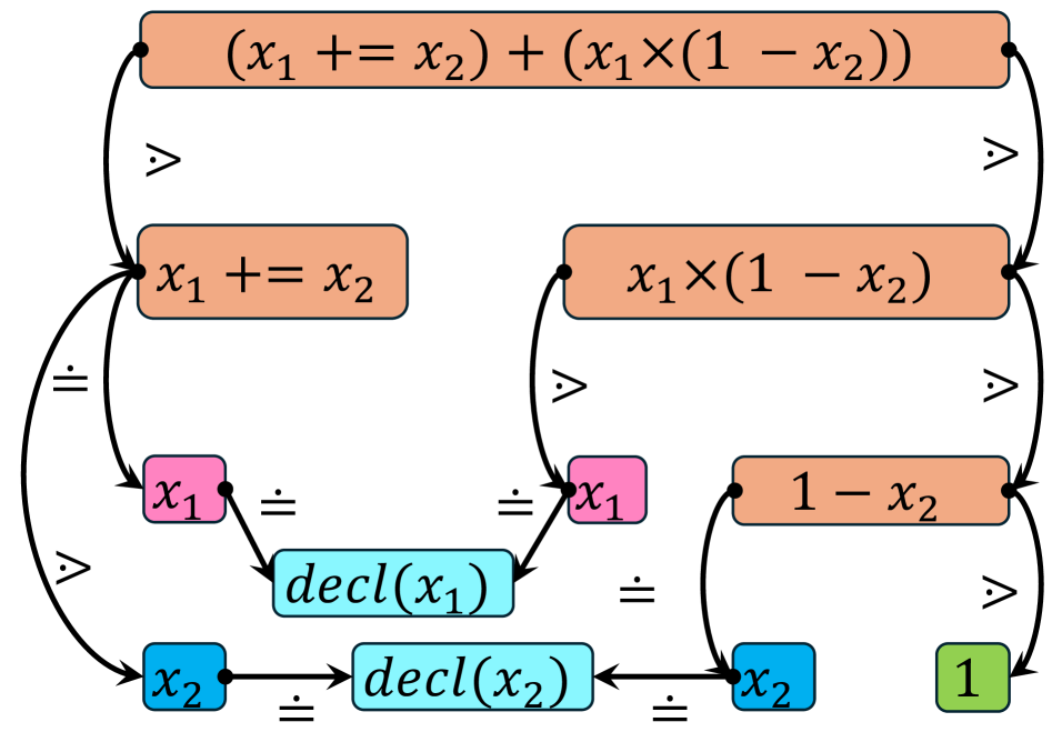
Figure 9. An Example of a CUG

Example.  Figure˜9 illustrates an example of a data type CUG originated from the constraints related to $(x_{1}\mathrel{+}\mspace{-0.5mu}=x_{2})+(x_{1}\times(1-x_{2}))$. In this graph, each node symbolizes an attribute variable, and the expression content within each node indicates the expression to which the attribute variable pertains. The edges connecting the nodes plus the edge labels represent the node constraint relations.

CUG Pruning.  Figure˜9 suggests that although a single expression can produce multiple expression nodes, the number of related declaration nodes is constrained by the number of declarations that the expression references. In practice, this number is significantly smaller than the number of expression nodes, especially when we discourage the generation of new declarations if suitable variables are already present in the context. Furthermore, in real-world test programs, only declarations necessitate attributes. Consequently, we can simplify the CUG by eliminating all expression nodes and their corresponding edges, and then reconstruct the connections among the remaining declaration nodes. Such simplicity requires the establishment of a new relation, the extended node constraint relation, which integrates the cumulative effect of the edge contents along a path.

Definition 3.7 (Extended Node Constraint Relation).

An extended node constraint relation represented by ${\color[rgb]{.75,0,.25}\xhookrightarrow{\bowtie}}$ indicates the presence of a path such that the cumulative effect of the edge contents along this path can be encapsulated by the symbol $\bowtie$. The set of possible extended relations is given by $\{{\color[rgb]{.75,0,.25}\xhookrightarrow{\lessdot}},{\color[rgb]{.75,0,.25}\xhookrightarrow{\gtrdot}},{\color[rgb]{.75,0,.25}\xhookrightarrow{\doteq}},{\color[rgb]{.75,0,.25}\xhookrightarrow{\mathrel{\gtrdot\mkern-4.0mu\lessdot}}}\}$. In this context: If $V_{{\color[rgb]{1,0,0}\mathscr{A}}_{i}}{\color[rgb]{.75,0,.25}\xhookrightarrow{\mathrel{\gtrdot\mkern-4.0mu\lessdot}}}V_{{\color[rgb]{1,0,0}\mathscr{A}}_{j}}$, it implies that the attribute variable ${\color[rgb]{1,0,0}\mathscr{A}}_{i}$ is either more restricted than ($\lessdot$) or less restricted than ($\gtrdot$) ${\color[rgb]{1,0,0}\mathscr{A}}_{j}$. ${\color[rgb]{.75,0,.25}\xhookrightarrow{\bowtie}}$ is defined by Figure˜10 where $\implies$ denotes "implies" and $\wedge$ denotes "and".

$$(V_{{\color[rgb]{1,0,0}\mathscr{A}}_{i}}{\color[rgb]{.75,0,.25}\xhookrightarrow{\bowtie_{ij}}}V_{{\color[rgb]{1,0,0}\mathscr{A}}_{j}}\wedge V_{{\color[rgb]{1,0,0}\mathscr{A}}_{j}}{\color[rgb]{.75,0,.25}\xhookrightarrow{\bowtie_{jk}}}V_{{\color[rgb]{1,0,0}\mathscr{A}}_{k}})\wedge V_{{\color[rgb]{1,0,0}\mathscr{A}}_{k}}{\color[rgb]{.75,0,.25}\xhookrightarrow{\bowtie_{kl}}}V_{{\color[rgb]{1,0,0}\mathscr{A}}_{l}}=V_{{\color[rgb]{1,0,0}\mathscr{A}}_{i}}{\color[rgb]{.75,0,.25}\xhookrightarrow{\bowtie_{ij}}}V_{{\color[rgb]{1,0,0}\mathscr{A}}_{j}}\wedge(V_{{\color[rgb]{1,0,0}\mathscr{A}}_{j}}{\color[rgb]{.75,0,.25}\xhookrightarrow{\bowtie_{jk}}}V_{{\color[rgb]{1,0,0}\mathscr{A}}_{k}}\wedge V_{{\color[rgb]{1,0,0}\mathscr{A}}_{k}}{\color[rgb]{.75,0,.25}\xhookrightarrow{\bowtie_{kl}}}V_{{\color[rgb]{1,0,0}\mathscr{A}}_{l}})\quad(\text{Associative})$$

$$V_{{\color[rgb]{1,0,0}\mathscr{A}}_{i}}{\color[rgb]{.75,0,.25}\xhookrightarrow{\bowtie_{ij}}}V_{{\color[rgb]{1,0,0}\mathscr{A}}_{j}}\wedge V_{{\color[rgb]{1,0,0}\mathscr{A}}_{j}}{\color[rgb]{.75,0,.25}\xhookrightarrow{\bowtie_{jk}}}V_{{\color[rgb]{1,0,0}\mathscr{A}}_{k}}\implies V_{{\color[rgb]{1,0,0}\mathscr{A}}_{j}}{\color[rgb]{.75,0,.25}\xhookrightarrow{\bowtie_{jk}}}V_{{\color[rgb]{1,0,0}\mathscr{A}}_{k}}\wedge V_{{\color[rgb]{1,0,0}\mathscr{A}}_{i}}{\color[rgb]{.75,0,.25}\xhookrightarrow{\bowtie_{ij}}}V_{{\color[rgb]{1,0,0}\mathscr{A}}_{j}}\quad(\text{Commutative})$$

$$\begin{aligned} \forall{\color[rgb]{.75,0,.25}\xhookrightarrow{\bowtie}}\in\{{\color[rgb]{.75,0,.25}\xhookrightarrow{\lessdot}},{\color[rgb]{.75,0,.25}\xhookrightarrow{\gtrdot}},{\color[rgb]{.75,0,.25}\xhookrightarrow{\doteq}},{\color[rgb]{.75,0,.25}\xhookrightarrow{\mathrel{\gtrdot\mkern-4.0mu\lessdot}}}\},&\quad V_{{\color[rgb]{1,0,0}\mathscr{A}}_{i}}{\color[rgb]{.75,0,.25}\xhookrightarrow{\bowtie}}V_{{\color[rgb]{1,0,0}\mathscr{A}}_{j}}\wedge V_{{\color[rgb]{1,0,0}\mathscr{A}}_{j}}{\color[rgb]{.75,0,.25}\xhookrightarrow{\bowtie}}V_{{\color[rgb]{1,0,0}\mathscr{A}}_{k}}\implies V_{{\color[rgb]{1,0,0}\mathscr{A}}_{i}}{\color[rgb]{.75,0,.25}\xhookrightarrow{\bowtie}}V_{{\color[rgb]{1,0,0}\mathscr{A}}_{k}}\quad(\text{Transitive})\\ \phantom{\forall{\color[rgb]{.75,0,.25}\xhookrightarrow{\bowtie}}\in\{{\color[rgb]{.75,0,.25}\xhookrightarrow{\lessdot}},{\color[rgb]{.75,0,.25}\xhookrightarrow{\gtrdot}},{\color[rgb]{.75,0,.25}\xhookrightarrow{\doteq}},{\color[rgb]{.75,0,.25}\xhookrightarrow{\mathrel{\gtrdot\mkern-4.0mu\lessdot}}}\},}&\quad V_{{\color[rgb]{1,0,0}\mathscr{A}}_{i}}{\color[rgb]{.75,0,.25}\xhookrightarrow{\doteq}}V_{{\color[rgb]{1,0,0}\mathscr{A}}_{j}}\wedge V_{{\color[rgb]{1,0,0}\mathscr{A}}_{j}}{\color[rgb]{.75,0,.25}\xhookrightarrow{\bowtie}}V_{{\color[rgb]{1,0,0}\mathscr{A}}_{k}}\implies V_{{\color[rgb]{1,0,0}\mathscr{A}}_{i}}{\color[rgb]{.75,0,.25}\xhookrightarrow{\bowtie}}V_{{\color[rgb]{1,0,0}\mathscr{A}}_{k}}\\ \phantom{\forall{\color[rgb]{.75,0,.25}\xhookrightarrow{\bowtie}}\in\{{\color[rgb]{.75,0,.25}\xhookrightarrow{\lessdot}},{\color[rgb]{.75,0,.25}\xhookrightarrow{\gtrdot}},{\color[rgb]{.75,0,.25}\xhookrightarrow{\doteq}},{\color[rgb]{.75,0,.25}\xhookrightarrow{\mathrel{\gtrdot\mkern-4.0mu\lessdot}}}\},}&\quad V_{{\color[rgb]{1,0,0}\mathscr{A}}_{i}}{\color[rgb]{.75,0,.25}\xhookrightarrow{\mathrel{\gtrdot\mkern-4.0mu\lessdot}}}V_{{\color[rgb]{1,0,0}\mathscr{A}}_{j}}\wedge V_{{\color[rgb]{1,0,0}\mathscr{A}}_{j}}{\color[rgb]{.75,0,.25}\xhookrightarrow{\bowtie}}V_{{\color[rgb]{1,0,0}\mathscr{A}}_{k}}\implies V_{{\color[rgb]{1,0,0}\mathscr{A}}_{i}}{\color[rgb]{.75,0,.25}\xhookrightarrow{\mathrel{\gtrdot\mkern-4.0mu\lessdot}}}V_{{\color[rgb]{1,0,0}\mathscr{A}}_{k}}\end{aligned}$$

$$V_{{\color[rgb]{1,0,0}\mathscr{A}}_{i}}{\color[rgb]{.75,0,.25}\xhookrightarrow{\lessdot}}V_{{\color[rgb]{1,0,0}\mathscr{A}}_{j}}\wedge V_{{\color[rgb]{1,0,0}\mathscr{A}}_{j}}{\color[rgb]{.75,0,.25}\xhookrightarrow{\gtrdot}}V_{{\color[rgb]{1,0,0}\mathscr{A}}_{k}}\implies V_{{\color[rgb]{1,0,0}\mathscr{A}}_{i}}{\color[rgb]{.75,0,.25}\xhookrightarrow{\mathrel{\gtrdot\mkern-4.0mu\lessdot}}}V_{{\color[rgb]{1,0,0}\mathscr{A}}_{k}}$$

Figure 10. Rules for Calculating Extended Node Constraint Relation

Algorithm 2 Algorithm for pruning CUG

1:procedure CUG_Prune($G$)

2:  $V_{e}\leftarrow\text{Get expression nodes from }G$

3:  for $v_{e}\in V_{e}$ do

4:   $V_{d}\leftarrow\text{Get declaration nodes connected by }v_{e}$

5:   for $(v_{d_{i}},v_{d_{j}})\in V_{d}\times V_{d}\ where\ {i<j}$ do

6:     $\text{Calculate }v_{e}{\color[rgb]{.75,0,.25}\xhookrightarrow{\bowtie_{i}}}v_{d_{i}}\text{ and }v_{e}{\color[rgb]{.75,0,.25}\xhookrightarrow{\bowtie_{j}}}v_{d_{j}}$

7:     $\text{Unify }{\color[rgb]{.75,0,.25}\xhookrightarrow{\bowtie_{i}}}\text{ and }{\color[rgb]{.75,0,.25}\xhookrightarrow{\bowtie_{j}}}\text{ into }{\color[rgb]{.75,0,.25}\xhookrightarrow{\bowtie_{ij}^{\prime}}}\text{ and connect }v_{d_{i}}\text{ and }v_{d_{j}}\text{ with it}$

8:     if ${\color[rgb]{.75,0,.25}\xhookrightarrow{\bowtie_{ij}}}$ not exists or ${\color[rgb]{.75,0,.25}\xhookrightarrow{\bowtie_{ij}^{\prime}}}\prec{\color[rgb]{.75,0,.25}\xhookrightarrow{\bowtie_{ij}}}$ then

9:      ${\color[rgb]{.75,0,.25}\xhookrightarrow{\bowtie_{ij}}}={\color[rgb]{.75,0,.25}\xhookrightarrow{\bowtie_{ij}^{\prime}}}$

10:     end if

11:   end for

12:  end for

13:end procedure

Algorithm˜2 describes the CUG pruning procedure. The algorithm iterates through each expression node (˜3) and then examines all pairs of declaration nodes linked by the expression node (˜5). For every such pair, the algorithm first calculates the extended node constraint relation from the expression node to each declaration node (˜6), and then establish an node constraint relation between the two declaration nodes (˜7) following the unifying rules in Figure˜11. Line 8-10 presents that if multiple edges labeled ${\color[rgb]{.75,0,.25}\xhookrightarrow{\bowtie_{ij}}}$ are present, select the one with the smallest value according to the partial order relation $\prec$, the definition of which is provided in Figure˜11.

$${\color[rgb]{.75,0,.25}\xhookrightarrow{\bowtie_{i}}}\ =\ {\color[rgb]{.75,0,.25}\xhookrightarrow{\mathrel{\gtrdot\mkern-4.0mu\lessdot}}}\lor{\color[rgb]{.75,0,.25}\xhookrightarrow{\bowtie_{j}}}\ =\ {\color[rgb]{.75,0,.25}\xhookrightarrow{\mathrel{\gtrdot\mkern-4.0mu\lessdot}}}\ \implies\ {\color[rgb]{.75,0,.25}\xhookrightarrow{\bowtie_{ij}}}\ =\ {\color[rgb]{.75,0,.25}\xhookrightarrow{\mathrel{\gtrdot\mkern-4.0mu\lessdot}}}$$

$${\color[rgb]{.75,0,.25}\xhookrightarrow{\bowtie_{i}}}\ =\ {\color[rgb]{.75,0,.25}\xhookrightarrow{\bowtie_{j}}}\ \implies\ {\color[rgb]{.75,0,.25}\xhookrightarrow{\bowtie_{ij}}}\ =\ {\color[rgb]{.75,0,.25}\xhookrightarrow{\doteq}}\text{ if }{\color[rgb]{.75,0,.25}\xhookrightarrow{\bowtie_{i}}}\ =\ {\color[rgb]{.75,0,.25}\xhookrightarrow{\doteq}}\text{ else }{\color[rgb]{.75,0,.25}\xhookrightarrow{\mathrel{\gtrdot\mkern-4.0mu\lessdot}}}$$

$${\color[rgb]{.75,0,.25}\xhookrightarrow{\bowtie_{i}}}\ \neq\ {\color[rgb]{.75,0,.25}\xhookrightarrow{\mathrel{\gtrdot\mkern-4.0mu\lessdot}}}\ \wedge\ {\color[rgb]{.75,0,.25}\xhookrightarrow{\bowtie_{j}}}\ \neq\ {\color[rgb]{.75,0,.25}\xhookrightarrow{\mathrel{\gtrdot\mkern-4.0mu\lessdot}}}\ \wedge\ {\color[rgb]{.75,0,.25}\xhookrightarrow{\bowtie_{i}}}\ \prec\ {\color[rgb]{.75,0,.25}\xhookrightarrow{\bowtie_{j}}}\ \implies\ {\color[rgb]{.75,0,.25}\xhookrightarrow{\bowtie_{ij}}}\ =\ {\color[rgb]{.75,0,.25}\xhookrightarrow{\gtrdot}}$$

$$\phantom{{\color[rgb]{.75,0,.25}\xhookrightarrow{\bowtie_{i}}}\ \neq\ {\color[rgb]{.75,0,.25}\xhookrightarrow{\mathrel{\gtrdot\mkern-4.0mu\lessdot}}}\ \wedge\ {\color[rgb]{.75,0,.25}\xhookrightarrow{\bowtie_{j}}}\ \neq\ {\color[rgb]{.75,0,.25}\xhookrightarrow{\mathrel{\gtrdot\mkern-4.0mu\lessdot}}}}\ \wedge\ {\color[rgb]{.75,0,.25}\xhookrightarrow{\bowtie_{j}}}\ \prec\ {\color[rgb]{.75,0,.25}\xhookrightarrow{\bowtie_{i}}}\ \implies\ {\color[rgb]{.75,0,.25}\xhookrightarrow{\bowtie_{ij}}}\ =\ {\color[rgb]{.75,0,.25}\xhookrightarrow{\lessdot}}$$

Figure 11. Unifying Rules, Where $\prec$ Is Defined by ${\color[rgb]{.75,0,.25}\xhookrightarrow{\lessdot}}\ \prec\ {\color[rgb]{.75,0,.25}\xhookrightarrow{\doteq}}\ \prec\ {\color[rgb]{.75,0,.25}\xhookrightarrow{\gtrdot}}$

Algorithm 3 Algorithm for collecting substitutions

1:$\sigma\leftarrow\{\}$

2:$\Sigma\leftarrow\{\}$

3:procedure collect_substitution($V_{{\color[rgb]{1,0,0}\mathscr{A}}_{i}}$)

4:  for $\upsilon\in{\color[rgb]{.75,.5,.25}\tau}_{{\color[rgb]{1,0,0}\mathscr{A}}_{i}}$ do

5:   $\sigma\leftarrow\sigma\bigcup\{{\color[rgb]{1,0,0}\mathscr{A}}_{i}\leftarrow v\}$

6:   if $\exists V_{{\color[rgb]{1,0,0}\mathscr{A}}_{j}},\ V_{{\color[rgb]{1,0,0}\mathscr{A}}_{i}}{\color[rgb]{.75,0,.25}\xhookrightarrow{\bowtie}}V_{{\color[rgb]{1,0,0}\mathscr{A}}_{j}}\ and\ {\color[rgb]{.75,.5,.25}\tau}_{{\color[rgb]{1,0,0}\mathscr{A}}_{j}}\backslash\{\kappa|\upsilon\not\bowtie_{ij}\kappa\}=\emptyset$ then

7:     continue

8:   end if

9:   for $V_{{\color[rgb]{1,0,0}\mathscr{A}}_{j}}\text{ such that }V_{{\color[rgb]{1,0,0}\mathscr{A}}_{i}}\ {\color[rgb]{.75,0,.25}\xhookrightarrow{\bowtie_{ij}}}\ V_{{\color[rgb]{1,0,0}\mathscr{A}}_{j}}$ do

10:     ${\color[rgb]{.75,.5,.25}\tau}_{{\color[rgb]{1,0,0}\mathscr{A}}_{j}}\leftarrow{\color[rgb]{.75,.5,.25}\tau}_{{\color[rgb]{1,0,0}\mathscr{A}}_{j}}\backslash\{\kappa|\upsilon\not\bowtie_{ij}\kappa\}$

11:   end for

12:   for $V_{{\color[rgb]{1,0,0}\mathscr{A}}_{j}}\text{ such that }V_{{\color[rgb]{1,0,0}\mathscr{A}}_{i}}\ {\color[rgb]{.75,0,.25}\xhookrightarrow{\bowtie_{ij}}}\ V_{{\color[rgb]{1,0,0}\mathscr{A}}_{j}}$ do

13:     collect_substitution($V_{{\color[rgb]{1,0,0}\mathscr{A}}_{j}}$)

14:   end for

15:   for $V_{{\color[rgb]{1,0,0}\mathscr{A}}_{j}}\text{ such that }V_{{\color[rgb]{1,0,0}\mathscr{A}}_{i}}\ {\color[rgb]{.75,0,.25}\xhookrightarrow{\bowtie_{ij}}}\ V_{{\color[rgb]{1,0,0}\mathscr{A}}_{j}}$ do

16:     ${\color[rgb]{.75,.5,.25}\tau}_{{\color[rgb]{1,0,0}\mathscr{A}}_{j}}\leftarrow{\color[rgb]{.75,.5,.25}\tau}_{{\color[rgb]{1,0,0}\mathscr{A}}_{j}}\bigcup\{\kappa|\upsilon\not\bowtie_{ij}\kappa\}$

17:   end for

18:   if $sz(\sigma)=\text{\# Attribute Variable}$ then

19:     $\Sigma\leftarrow\Sigma\bigcup\{\sigma\}$

20:   end if

21:   $\sigma\leftarrow\sigma\backslash\{{\color[rgb]{1,0,0}\mathscr{A}}_{i}\leftarrow v\}$

22:  end for

23:end procedure

Substitution Collection.  After pruning the CUG, the next step is to collect the substitutions that unify the pruned CUG. The substitution collection algorithm is detailed in Algorithm˜3. The algorithm begins by initializing $\sigma$ and $\Sigma$ to empty sets (˜1 and ˜2) where $\sigma$ is a substitution while $\Sigma$ is a set of substitutions. The algorithm proceeds to traverse each value $\upsilon$ from node $V_{{\color[rgb]{1,0,0}\mathscr{A}}_{i}}$’s codomain ${\color[rgb]{.75,.5,.25}\tau}_{{\color[rgb]{1,0,0}\mathscr{A}}_{i}}$ (˜4) and updates $\sigma$ by assigning value $\upsilon$ to attribute variable ${\color[rgb]{1,0,0}\mathscr{A}}_{i}$ (˜5). Line 6-8 checks if the choice of $\upsilon$ narrows down any of the child’s attribute value codomain to an empty set. If so, the algorithm skips the current iteration since $\upsilon$ results in an unsolvable constraint. Line 9-11 updates the attribute value codomain of each child node $V_{{\color[rgb]{1,0,0}\mathscr{A}}_{j}}$ by removing all values that do not satisfy the node constraint relation $V_{{\color[rgb]{1,0,0}\mathscr{A}}_{i}}{\color[rgb]{.75,0,.25}\xhookrightarrow{\bowtie_{ij}}}V_{{\color[rgb]{1,0,0}\mathscr{A}}_{j}}$. Line 12-14 recursively calls the substitution collection algorithm on the child node $V_{{\color[rgb]{1,0,0}\mathscr{A}}_{j}}$ to collect substitutions for the node. Line 15-17 restores the value codomain of each child node $V_{{\color[rgb]{1,0,0}\mathscr{A}}_{j}}$ by adding back all values that do not satisfy the node constraint relation $V_{{\color[rgb]{1,0,0}\mathscr{A}}_{i}}{\color[rgb]{.75,0,.25}\xhookrightarrow{\bowtie_{ij}}}V_{{\color[rgb]{1,0,0}\mathscr{A}}_{j}}$. Finally, the algorithm updates $\Sigma$ with the current substitution $\sigma$ (˜19) if $\sigma$ contains value assignments to all attribute variables, and rollback the update to $\sigma$ (˜21).

Search Space.  The substitution collection algorithm examines the entire space of potential substitutions and eliminates those that fail to unify the constraints. For the pruned CUG $G_{p}$, the size of the search space is given by $\prod_{d\in\mathcal{D}}\|R_{d}\|$, where $\mathcal{D}$ represents the set of declaration nodes in the CUG and $\|R_{d}\|$ means the size of the value codomain of each declaration node. In contrast, for the original CUG $G$, the search space size is $\prod_{d\in\mathcal{D}}\|R_{d}\|\times\prod_{e\in\mathcal{E}}\|R_{e}\|$, where $\mathcal{E}$ denotes the set of expression nodes in the CUG. The pruning of the CUG reduces the search space by a factor of $\prod_{e\in\mathcal{E}}\|R_{e}\|$, which is attributed to the elimination of expression nodes and their associated substitution possibilities.

$G_{p}$-Solvability.  The pruned CUG $G_{p}$ consistently results in non-empty substitution sets when using the substitution collection algorithm. Assume that the constraint system ${\color[rgb]{.5,0,.5}\mathbb{C}}$ can be expanded to ${\color[rgb]{.5,0,.5}\mathbb{C}}_{ex}$ by progressively combining pairs of constraints into new constraints using $\wedge$ defined in Figure˜10 until all constraints are incorporated. Since ${\color[rgb]{.5,0,.5}\mathbb{C}}$ is solvable, its extension ${\color[rgb]{.5,0,.5}\mathbb{C}}_{ex}$ must also be solvable. Now, consider another constraint set ${\color[rgb]{.5,0,.5}\mathbb{C}}_{p}$, which is derived by removing all attribute variables for expressions from ${\color[rgb]{.5,0,.5}\mathbb{C}}$ and retaining only those constraints that are directly related to the attribute variables associated with declarations. Because ${\color[rgb]{.5,0,.5}\mathbb{C}}_{p}\subseteq{\color[rgb]{.5,0,.5}\mathbb{C}}_{ex}$, it follows that ${\color[rgb]{.5,0,.5}\mathbb{C}}_{p}$ is also solvable. Furthermore, the pruning algorithm (Algorithm˜2) guarantees that the connections between nodes in the pruned CUG $G_{p}$ align with the relationships between declaration nodes in the original CUG $G$. Additionally, $G$ is semantically equivalent to ${\color[rgb]{.5,0,.5}\mathbb{C}}$ with respect to the relationships among attribute variables. Consequently, $G_{p}$ is semantically equivalent to ${\color[rgb]{.5,0,.5}\mathbb{C}}_{p}$. Since ${\color[rgb]{.5,0,.5}\mathbb{C}}_{p}$ is solvable, the substitution collection algorithm applied to $G_{p}$ will yield non-empty substitution sets.

4. Experimental Setup

Our experimental setup is designed to answer the following research questions:

RQ1:

How effective and efficient is Erwin in generating bug-triggered test programs?

RQ2:

How does Erwin compare to the state-of-the-art bug detection tools for Solidity compilers?

RQ3:

Do the main components of Erwin enhance bug detection in Solidity compilers?

4.1. Baselines

We select the following state-of-the-art bug detection tools for Solidity compilers as baselines:

AFL-compiler-fuzzer (ACF) (Groce et al., 2022):

ACF is an AFL-based mutation-based fuzzer that can be applied for Solidity compiler bug detection. ACF enhances AFL by incorporating several language-agnostic mutation rules (e.g., modifying conditions in if statements, deleting statements, etc.) tailored for common code structures. Additionally, ACF can assemble code fragments into new test cases, helping to diversify the seed pool and reuse code segments that have previously revealed bugs.

Fuzzol (Mitropoulos et al., 2024):

Fuzzol is a mutation-based fuzzer designed specifically for the Solidity compiler. Unlike ACF, Fuzzol distinguishes itself by integrating language-specific mutators. It begins by analyzing the abstract syntax trees (ASTs) of Solidity test cases and then applies mutators to specific AST nodes. For example, Fuzzol may replace an AST node with another node of the same type or adjust the arguments of an opcode within an inline assembly node. This strategy allows Fuzzol to deliver more targeted and language-aware mutations, significantly enhancing the effectiveness of the fuzzing process.

4.2. Systems Under Test

We apply Erwin, ACF and Fuzzol to the following compilers and analyzer:

solc (Sol, 2025b):

The main compiler for Solidity, solc is a crucial tool for developers working with the Ethereum blockchain. It compiles Solidity into Ethereum Virtual Machine (EVM) bytecode. This bytecode is then deployed and executed on the Ethereum network. The compiler ensures that the code adheres to the syntax and semantics of Solidity, providing error checking and optimization features.

solang (Sol, 2025a):

solang is another Solidity compiler that offers support for multiple blockchain platforms, including Ethereum, Solana, and Polkadot, providing greater flexibility for developers working across different ecosystems. While solc is the official Solidity compiler primarily focused on Ethereum and EVM-compatible blockchains, solang aims to offer a more versatile compilation process with an emphasis on performance optimizations and modern development practices.

slither (Sli, 2025):

slither is a static analysis tool designed for Solidity. It is primarily used to detect vulnerabilities and bugs in smart contracts by analyzing the code without executing it. slither provides a comprehensive analysis of the contract’s structure, control flow, and data flow, helping developers identify potential security issues, such as reentrancy, integer overflows, and improper access controls. Though slither is not a compiler, it can accept Solidity code as input and thus we select it for testing.

4.3. Metrics

Our evaluation is mainly based on the following widely-used metrics:

Code Coverage:

Following previous work (Liu et al., 2023; Böhme et al., 2017; Even-Mendoza et al., 2023), we trace the source-level line coverage and edge coverage of the entire solc codebase, the most popular Solidity compiler that sets the language standard. We exclude the solang compiler from the study because its slightly different Solidity grammar would render test program mutation ineffective in the two baseline approaches, resulting in an unfair comparison with Erwin.

Bug Count:

Following previous work (Ma et al., 2023; Wang et al., 2024; Suo et al., 2024; Shen et al., 2025), we measure the number of bugs detected by Erwin and use it to measure the effectiveness of Erwin. When counting new bugs, a potential bug is caught if it leads to an unexpected crash (e.g., a segmentation fault) or incorrect behavior (e.g., an assertion failure without a clear error message). Additionally, developers’ confirmation and code patches addressing the issue serve as strong indicators that the issue is indeed a bug. When counting bugs detected by Erwin in a Solidity compiler bug dataset (Ma et al., 2024), we compare the error message of the detected issue with the error message of the corresponding bug documented in the dataset. If the two error messages are either identical or differ only slightly (e.g., in details such as the length of an array), we classify the detected issue as a unique bug from the dataset.

4.4. Implementation

Our Erwin tool comprises 15,098 lines of TypeScript code. While Erwin is designed to be easily extensible to cover the full range of Solidity language features, the current version (1.3.1) only supports a limited subset of these features, including contracts, functions, modifiers, events, errors, etc. The support for other features (e.g., interface, library, contract inheritance, and inline assembly) will be added in future versions of Erwin.

Given the differences in Solidity grammar across various versions and compilers, Erwin is developed using the Solidity grammar from solc version 0.8.20. This grammar is not universally applicable but is compatible with a broad range of Solidity versions. Furthermore, we have extended Erwin to support the grammar of solang version 0.3.3, enhancing its compatibility across different Solidity compiler ecosystems.

4.5. Experimental Configuration

The testbed hardware configuration includes 1) AMD Ryzen Threadripper 3970X 32-Core Processor (64 threads, 2200Mhz - 3700 Mhz), 2) 256 GB RAM (3200 Mhz), and 3) Samsung SSD 970 EVO Plus 2TB. The operating system is AlmaLinux 9.5. We conducted bug detection process on various versions, including solc 0.8.20-0.8.28, solang 0.3.3, and slither 0.10.4.

Since Erwin’s generation process involves randomness, we expose all random variables as configurable flags. During evaluation, we integrate a random flag selection script into Erwin to prevent bias towards particular random seeds and ensure the evaluation’s fairness. This script can explore all possible and valid combinations of random flags, providing a comprehensive evaluation of Erwin’s performance.

5. Evaluation

5.1. RQ1: Effectiveness of Erwin

5.1.1. Case Study of Detected Bugs

Table 1. Status of Reported Bugs in
solc, solang, and slither

	Bugs	Confirmed	Fixed	Duplicate
solc	21	15	8	3
solang	4	0	0	0
slither	1	1	1	0
Total	26	16	9	3

After six months of intermittent operation, Erwin has identified a total of 26 bugs across solc, solang, and slither. Table˜1 provides a detailed breakdown of the bugs detected by Erwin in each system under test. Out of these, 16 have been confirmed as bugs by developers, and nine of those have already been fixed. The remaining bugs, including six bugs for solc and four bugs for solang, are still under investigation. Among the 16 confirmed bugs, three solc bugs are categorized as duplicates by developers. The 13 non-duplicate confirmed bugs have various symptoms and root causes. In terms of symptoms, two bugs trigger segmentation fault, four bugs lead to incorrect output, one bug results in hang, five bugs induce internal compiler error (ICE), and one bug causes the compiler to accept invalid programs. As for root causes, two bugs are caused by type errors, three bugs are related to incorrect error handling, four bugs are due to formal verification errors, one bug is caused by code analysis error, one bug is due to incorrect version control, and two bugs are caused by specification errors.

⬇

1bool internal v;

2modifier m() {

3 while (v ? false : v) {}

4 _;

5}

Example 1: Test Program for GitHub Issue #2619 (bug, 2025a)

Code Analysis Error $+$ Hang.  The GitHub issue 2619 (bug, 2025a) is a code analysis error that causes slither to hang. LABEL:listing:bug2619 shows the bug-triggered fragment inside a contract for this issue. The bug arises from the code analysis process, where slither statically analyzes the code to detect vulnerabilities. The bug-triggered scenario involves a modifier that contains a while loop, where the loop’s condition expression is a ternary operation over an uninitialized boolean member variable. If the while loop is moved into a function or the ternary operation expression is altered, the bug will not be detected during analysis.

Formal Verification Error $+$ ICE.  The GitHub issue 15647 exposes a formal verification error that causes an Internal Compiler Error (ICE) in the solc compiler. LABEL:listing:bug15647 shows the bug-triggered test program for this issue. The formal verification component is a specialized feature of the solc compiler designed to confirm the accuracy of smart contract code and ensure its behavior aligns with the specified requirements. The formal verification process involves two primary stages: SMT encoding and solving (Ma et al., 2024). During SMT encoding, the smart contract code is transformed into a logical formula IR. This formula is then analyzed by an SMT solver to ascertain the code’s correctness.

⬇

1contract C {

2 constructor() {

3 int128 v;

4 (v *= v);

5 }

6 bool[6] internal arr;

7 function f() internal {

8 while(arr[(3)] == true) {}

9 }

10}

Example 2: Test Program for GitHub Issue #15647 (bug, 2025b)

This particular bug is deeply buried within the SMT encoding process, where the compiler mishandles array access expressions. Although the root cause appears straightforward, the bug is exceptionally difficult to detect because it only manifests under specific conditions: when an boolean array access expression is located within the condition of a while loop or a do while loop inside an internal function. Additionally, triggering the bug requires the presence of a constructor that includes a multiplication assignment operation. Erwin has the ability to generate intricate test programs and investigate various data types and function visibilities. Consequently, Erwin can thoroughly explore the potential combinations of array types and function visibilities, ultimately leading to the identification of this bug.

⬇

1contract C {

2 struct S {

3 bool b;

4 }

5}

6contract D {

7 C.S public s;

8

9 function func14() public view {

10 true ? C.S(true) : this.s();

11 }

12}

Example 3: Test Program for GitHub Issue #15525 (bug, 2025g)

Specification Error $+$ ICE.  The GitHub issue 15525 is a specification error that results in the solc compiler incorrectly crashing. LABEL:listing:bug15525 shows the bug-triggered test program for this issue. The issue stems from the compiler’s peculiar handling of the getter function for a state variable of struct type. In the code, the expression C.S(true) on line 10 is a constructor call that generates a new instance of the struct type C.S. When the program attempts to retrieve s using this.s(), the compiler erroneously returns a tuple containing the struct’s members instead of the struct itself. This quirk leads to a type mismatch, causing a compilation error on line 10. Developers have confirmed that this issue is a long-standing quirk and will address it in the future breaking change. They agree that the current Solidity specification lacks clarity, which accounts for the occurrence of such issues. With formalizing the Solidity specification, Erwin can explore all possible language features and their interactions, thus uncovering this bug.

5.1.2. Coverage Enhancement

As the most popular Solidity compiler and the initial compiler for Solidity language, solc has been widely adopted by smart contract developers. To evaluate the effectiveness of Erwin in generating high-quality bug-triggered test programs, we compare the line and edge coverage of solc using test programs generated by Erwin within 24 hours and unit test cases.

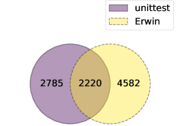
(a) Edge Coverage Difference

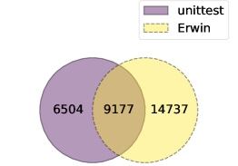
(b) Line Coverage Difference

Figure 12. Edge and Line Coverage Difference Among Erwin’s generated test programs and Unit Tests

Figure˜12(a) and 12(b) show the Venn diagrams of the edge and line coverage differences among Erwin’s generated test programs and unit test. The results show that Erwin can cover 4,582 edges and 14,737 lines that are not covered by unit test cases.

5.1.3. Throughput and Efficiency

Table 2. Througput of IR and Programs generation

gen	1	50	100	150	200	250	300	350	400
IR Programs / s	65.53	13.78	8.53	5.84	2.13	1.98	1.65	1.58	1.34
Programs / s	65.53	689.00	853.53	876.17	427.62	496.13	494.76	553.02	537.77

To assess the efficiency of Erwin in producing test programs, we evaluate the throughput of Erwin in generating both IR programs and the subsequent test programs by executing Erwin under each generation setting for 1000 times under Erwin’s -max flag for acceleration. We repeat the experiment five times and calculate the median throughput values to ensure the reliability of the results. Table 2 presents the throughput of Erwin. The gen row indicates the quantity of test programs lowered from the generated IR programs. To guarantee that the IR programs can be lowered into this number of test programs, we configure Erwin to generate two contracts, each containing two member functions. This configuration aims to enhance the program’s complexity and, consequently, the size of the search space. The gen1 case is a special scenario where Erwin halts subsitution collection process (Algorithm˜3) in the search space upon discovering the first valid combination. The throughput, measured at 65.53 test programs per second, demonstrates that Erwin is capable of rapidly generating IR test programs and effectively solving constraints to produce the desired test programs. As the suffix number in gen increases, the data for IR programs generated per second intuitively declines. This is because Erwin requires additional time to collect more substitutions for the IR program, thereby increasing the computational effort and reducing the overall throughput for IR program generation. Regarding programs per second, the throughput initially rises from gen1 to gen150 and then experiences a sudden decrease, fluctuating between 420 and 560. This decrease suggests that as the number of required test programs grows, the substitution collection algorithm (Algorithm 3) requires more time to identify a new substitution that satisfies all constraints. The table implies that gen50, gen100, and gen150 are optimal configurations for generating test programs, as they yield the highest throughput values.

5.2. RQ2: Comparison with State-of-the-Art Fuzzing Tools

We evaluate Erwin against two cutting-edge fuzzing tools for Solidity compilers, ACF and Fuzzol, by comparing the number of bugs detected in the Solidity compiler bugs dataset. This dataset includes 104 reproducible bugs that manifest as crashes in the Solidity compiler (solc).

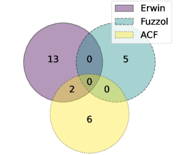
(a) Bug Detection Difference

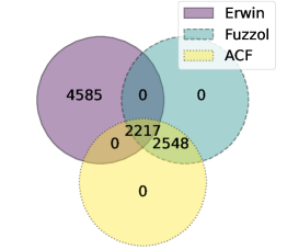
(b) Edge Coverage Difference

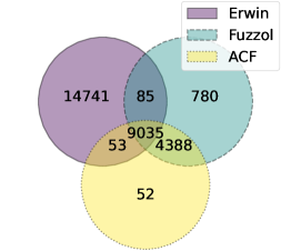
(c) Line Coverage Difference

Figure 13. Effectiveness Differences Among Erwin, ACF, and Fuzzol

Figure˜13(a) shows the bug detection difference among Erwin, ACF, and Fuzzol in the Solidity compiler bugs dataset after executing them for 20 days separately. The seed pool for ACF and Fuzzol is set following their default configurations (Groce et al., 2022; Mitropoulos et al., 2024). The results show that Erwin can detect 15 bugs in total, of which 13 bugs are not detected by ACF and Fuzzol. Besides, Erwin also found a segmentation fault bug in solc 0.7.5 that is not in the dataset and not detected by ACF and Fuzzol. Of the 13 bugs detected, nine are due to formal verification errors, two stem from code generation errors, one is a type system error, and one is a memory-related error. The predominant formal verification errors have been observed to be particularly challenging for ACF and Fuzzol to detect (Ma et al., 2024). As the formal verification component relies on SMT encoding, it is highly sensitive to attribute values. Any misinterpretation of attributes can result in SMT encoding errors. Additionally, since the SMT solving process analyzes both control flow and data flow, conditions and loops are crucial for detecting formal verification errors. For instance, Erwin’s ability to generate complex test programs with intricate control flow and data flow and the ability to explore various attribute values and their interactions enables it to effectively detect formal verification errors. For instance, the bug 8963 in the dataset exposes a formal verification error that causes an ICE in the solc compiler. The bug-triggered scenario includes a tuple type or mapping type plus an assignment operation performed on its instance on line 5, and an if condition that enclose the assignment on line 4. Erwin can generate the if statement and explore the data type of $v$ on the left-hand side of the assignment, thereby uncovering this formal verification error.

⬇

1pragma experimental SMTChecker;

2contract C {

3 function f(int128 v) public{

4 if (1 == 1) {

5 (v) >>= 14235;

6 }

7 }

8}

Example 4: Test Program for GitHub Issue #8963 (bug, 2025d)

The 104 bugs in the dataset require various features: 12 need byte type, ten contract inheritance, eight library, six array pop/push, five each for fixed type, abi.encode, and Solidity grammar violations, four each for function type and inherent function calls, three each for inline assembly and type alias, two each for try catch, multiple test files, and enum, and one for comments. Erwin does not support these features for now so it cannot detect these 72 bugs. The lack of support for these features is also why Erwin failed to detect 11 bugs found by ACF and Fuzzol. In summary, Erwin detected 15 out of 32 bugs that are not dependent on language featuress currently unsupported by Erwin. With extended testing time and expanded feature support, the potential for discovering additional bugs is significant. Besides bug-detection differences, Figure˜13(b) and 13(c) show the Venn diagrams of the edge and line coverage differences among Erwin, ACF, and Fuzzol after 24-hour execution. The results show that Erwin can cover 4,585 edges and 14,741 lines that are not covered by ACF and Fuzzol. It’s noteworthy that Erwin can cover all edges covered by ACF and Fuzzol.

5.3. RQ3: Ablation Study

To evaluate the effectiveness of the main components of Erwin in enhancing bug detection in Solidity compilers, we conduct an ablation study by comparing the bug detection performance of Erwin with and without the main components.

5.3.1. Impact of the Attribute Value Exploration

In assessing Erwin’s approach to bounded exhaustive random program generation via attribute value exploration, we compare Erwin with a version that does not employ this strategy, which we refer to as ‘trivial Erwin’, denoted as Erwin_t. Due to the challenges in developing an alternative program generator based on Csmith’s approach, we configure Erwin_t to halt the constraint-solving process immediately upon finding a valid substitution that unify all constraints. To ensure a fair performance comparison, we exclude the time spent on constructing the CUG and performing CUG pruning from the measurements. Instead, we only account for the time taken for IR program generation, which is comparable to that of direct test programs generation. This approach isolates the impact of the IR generation and lowering strategy on Erwin_t’s performance. Since the generation process is stochastic, we repeat the experiment five times and calculate the median coverage values at each time stamp after linear interpolation to ensure the reliability of the results.

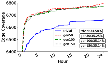
(a) Edge Coverage over Time

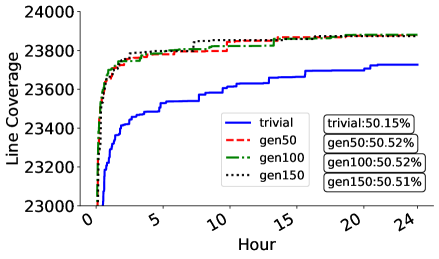
(b) Line Coverage over Time

Figure 14. Edge and Line Coverage over Time , Where the Percentages in the Figures Refer to Coverage Ratios

Figure˜14(a) and 14(b) illustrate the progression of edge and line coverage achieved by Erwin across various attribute value exploration configurations, as well as by Erwin_t. Erwin_t’s results are labeled as trivial in the figure, while gen50, gen100, and gen150 indicate that Erwin produces up to 50, 100, and 150 test programs, respectively, by examining attribute value combinations from the IR program. These three configurations establish the upper limit for the exhaustive attribute value exploration and exhibit different preferences in balancing the time spent exploiting the generated IR program against the time spent creating new ones. The figures evidently show that Erwin outperforms Erwin_t in both edge and line coverage across all selected configurations. Besides, though gen50, gen100, and gen150 achieve nearly the same line coverage, gen50 surpasses the other two in terms of edge coverage. This result suggests that the attribute value exploration strategy is crucial for enhancing the effectiveness of Erwin and consequently improving the bug detection performance. Besides, the results also indicate that the attribute value exploration strategy can be further optimized by adjusting the number of test programs generated from the IR program.

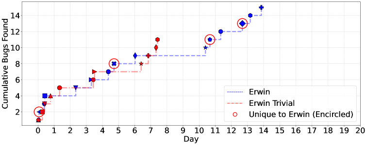
Figure 15. Erwin vs. Erwin_t in Bug Detection on the Solidity compiler Bugs Dataset

To further investigate the consequence of coverage difference between Erwin and Erwin_t, we expand the experiment in section˜5.2 by executing Erwin_t for 20 days on the Solidity compiler bugs dataset and compare the bug detection performance of Erwin with Erwin_t. The results are shown in Figure˜15, where different shapes represent different bugs detected by Erwin and Erwin_t. Since gen50 achieves the highest edge coverage, we choose it as the representative configuration for Erwin in the comparison. In general, Erwin_t is capable of identifying 11 bugs, all of which are

⬇

1pragma experimental ABIEncoderV2;

2contract C {

3 struct S { int[][5] c; }

4 S s;

5 function f(S calldata c) external {

6 s = c;

7 }

8}

Example 5: Test Program for GitHub Issue #10105 (bug, 2025e)

also found by Erwin. However, Erwin has a broader detection capability, identifying a total of 15 bugs, including four bugs that Erwin_t misses. We encircle them in the figure for clarity. The test programs that trigger these four bugs demand precise combinations of attribute values to meet the bug-triggered conditions, posing a significant challenge for Erwin_t. For example, consider bug 10105 (referenced as an encircled blue star in Figure˜15. This bug necessitates 1) a struct type that includes a nested array type, and 2) a non-internal function that takes the struct-type instance, stored in calldata, as a parameter (as illustrated in LABEL:listing:bug10105). The stringent requirements for data type, visibility, and storage location make it difficult to satisfy the conditions. Although Erwin_t might generate test programs that are similar in structure, differing only in the storage location of the struct-type instance, it still fails to meet the necessary conditions to trigger the bug. In contrast, Erwin excels in exploring all possible attribute values and their interactions, enabling it to uncover this bug effectively. The bug in Figure˜1, illustrated in section˜2.1 is another example of a bug that Erwin can detect on day five but Erwin_t cannot.

It is noteworthy that Erwin_t fails to detect any new bugs beyond the $8^{\text{th}}$ day, whereas Erwin successfully identifies six additional bugs during this period. Among the six bugs, four of which are also detected by Erwin_t. This bug detection delay arises because Erwin dedicates a portion of its effort to exploring attribute values.

Table 3. Search Space Size Reduction by CUG Pruning

	Median	Min	Max
Type	1.1e14	8	6.9e68
Storage	4.5e6	1	1.6e38
Visibility	1	1	1
Mutability	1	1	1

5.3.2. Impact of the CUG Pruning

CUG pruning, as outlined in Algorithm 2, constitutes a pivotal element of Erwin that seeks to diminish the search space and enhance the efficiency of bug detection. To assess the impact of CUG pruning on Erwin’s performance, we conducted Erwin for 1000 iterations and contrasted the average search space sizes of the CUG and the pruned CUG. Table 3 delineates the degree to which the search space size of the CUG surpasses that of the pruned CUG ($sz(G)/sz(G_{p})$). Given that the pruning of the CUG reduces the search space size by a factor of $\prod_{e\in\mathcal{E}}\|R_{e}\|$, the average size of the value codomain set $\|R_{e}\|$ for expression nodes $\mathcal{E}$ is crucial for achieving search space reduction. Since the majority of expressions are associated with data types and the $\|R_{e}\|$ for data types exceeds that of other attributes (as depicted in Figure 4), the reduction in search space size for data types is more pronounced compared to other attributes. Furthermore, because visibility and mutability constraint rules are not carried out by relations, CUG pruning does not impact the search space size for them.

6. Discussion

6.1. Threats to Validity

Although bounded exhaustive random program generation can alleviate certain inefficiencies stemming from opportunism, the inherent randomness in generating IR programs may still introduce opportunistic elements, potentially compromising the credibility of the experimental results. To address this issue, we implement two strategies: 1) we conduct each experiment multiple times and use the median value to represent the final outcomes, and 2) we prolong the testing duration to ensure that the bug-detection capabilities of Erwin and the baseline methods are thoroughly examined. This approach helps minimize the effects of randomness and enhances the reliability of the results. The first strategy is employed in several experiments, including the evaluation of solc coverage enhancement (Figure˜12), the throughput analysis (Table˜2), the comparison of Erwin under various generation settings (Figure˜14), and the comparison of Erwin with baseline methods in terms of code coverage (Figure˜13(b), Figure˜13(c)). In these experiments, each test is repeated five times, and the median values are reported to ensure robust results. The second strategy is utilized in the comparison between Erwin and Erwin_t (Figure˜15) and the comparison of Erwin with baseline methods in bug detection (Figure˜13(a)), where each experiment is conducted for 20 days.

6.2. False Alarms

While Erwin is built on the Solidity language specification and all its constraints are derived from this specification, there is still a chance that the generated programs may not be valid Solidity code. This invalidity can lead to the rejection of the generated programs by compilers, resulting in false alarms. These false alarms may arise from implementation errors in Erwin or, more significantly, from inaccuracies or ambiguities in the language specification itself. As of now, Erwin has identified three suspicious false alarms, two of which have been confirmed as errors in the specification. Consider GitHub issue 15483 (bug, 2025f) as an example. Its test program includes a function return declaration stored in calldata. While solc enforces that calldata return declarations must be assigned before use, this requirement is not explicitly mentioned in the Solidity language specification. Although developers from the solc team argue that this behavior is intentional rather than a bug, they acknowledge the inconsistency between the specification and the compiler implementation. This discrepancy has since been resolved. The identification of these two specification errors suggests that Erwin possesses not only the ability to detect bugs but also the potential to uncover deficiencies in the Solidity language specification. This capability is essential for refining the language specification and ensuring its alignment with the compiler implementation.

6.3. Seed Pool Enhancement

Program generators can serve a dual purpose: not only can they create test programs to uncover bugs in the system being tested, but they can also be utilized to enrich the seed pool for mutation-based fuzzers. For example, Csmith (Yang et al., 2011) is frequently employed to build a seed pool for mutation-based fuzzers like Athena (Le et al., 2015), Hermes (Sun et al., 2016), and GrayC (Even-Mendoza et al., 2023), , which are designed to test compilers like GCC and LLVM. These fuzzers then take the seed programs generated by Csmith and apply mutations to them. This process aims to uncover potential bug-hunting ability from test programs that did not initially trigger any issues in the system under test. We envision a similar approach for Solidity compilers, where Erwin can be used to generate test programs that can be fed into mutation-based fuzzers to enhance their seed pool. This approach may help mutation-based fuzzers to explore a broader range of test programs and potentially uncover more bugs in Solidity compilers. We extend the evaluation in section˜5.2 to explore how Erwin can enhance the seed pool for mutation-based fuzzers like ACF and Fuzzol, thereby improving their ability to detect bugs. Specifically, we configure Erwin in the gen1 mode to generate test programs, which are then added to the seed pools of ACF and Fuzzol. After each addition, we run these fuzzers for 24 hours, repeating this process over a span of 20 days. The results demonstrate that ACF and Fuzzol, when combined, can cover 112 lines and four edges that are not covered by unit tests or Erwin alone. This improvement in coverage enables the discovery of a bug in the dataset that was missed by Erwin and the two fuzzers without the inclusion of Erwin’s seed programs.

7. Related Work

7.1. Program Generation

Program generators are tools that automatically generates programs based on hard-coded rules or user-defined specifications (Ma, 2023; Chen et al., 2020). They can be utilized to generate test programs for testing the correctness of the compiler. For example, Csmith (Yang et al., 2011) is a random program generator for C programs based on Randprog (Eide and Regehr, 2008). Csmith can generate C programs from scratch containing struct, pointers, arrays, and other C features without undefined behaviors. By performing differential testing with the generated programs on GCC and LLVM, Csmith has found 325 previously unknown bugs in the target compilers as of the paper’s publication date. The success of Csmith in finding bugs in the GCC compiler has inspired the development of Csmith-family generators, such as CsmithEdge (Even-Mendoza et al., 2022), CUDAsmith (Jiang et al., 2020), nnsmith (Liu et al., 2023), and MLIRsmith (Wang et al., 2024), which are designed to test a variety of compilers. However, researchers have identified several inherent limitations in Csmith. These include susceptibility to saturation (Livinskii et al., 2020) and challenges in transferring its functionality to other languages (Chaliasos et al., 2022) To resolve the first limitation, yarpgen (Livinskii et al., 2020) proposes generation policies to skew the probability distribution of program ingredients. This approach can increase the diversity of the generated programs and delay the saturation point of the generator, beyond which the generator can no longer produce new programs and cannot find new bugs. To increase the range of the generator, Hephaestus (Chaliasos et al., 2022) proposes an IR which can be lowered to multiple languages, including Java, Kotlin, Scala, and Groovy. Although this method offers broader applicability, it sacrifices some of the specialized knowledge of a particular language, potentially resulting in the oversight of certain language-specific bugs. Erwin’s IR implementation is specialized for Solidity, which allows us to leverage the language-specific knowledge to generate Solidity programs with a higher likelihood of finding Solidity-specific bugs.

7.2. Template-based Compiler Testing

Template-based compiler testing is a technique that uses templates to generate programs for testing compilers. The templates are incomplete test programs that contain holes, which are filled with random values to create complete test programs. By leveraging templates, testing tools can harness the knowledge embedded within them, thereby reducing the effort required to generate programs from the ground up. JAttack (Zang et al., 2023a) is a testing tool that utilizes templates for JIT Java compilers. It necessitates developers to manually craft templates and can populate these templates with random values to guarantee the validity of the generated programs. SPE (Zhang et al., 2017) is capable of extracting templates from C test programs by substituting variables with placeholders or "holes." It then systematically explores all possible patterns of variable usage to alter the original dependencies among variables. SPE is a straightforward yet effective method for thoroughly investigating the potential to trigger bugs in programs produced by generators. MLIRsmith (Wang et al., 2024) is a program generator for MLIR that combines a template generation phase with a template instantiation phase to create MLIR programs. This two-phase generation strategy enhances the extensibility of MLIR program generation, allowing for the incorporation of expert knowledge through human-provided templates during the fuzzing process. Erwin’s IR can be regarded as a template for Solidity programs. Unlike JAttack, which necessitates manually crafted templates, Erwin has the capability to autonomously generate IR programs from the ground up. In contrast to SPE, which examines every possible pattern of variable usage, Erwin can investigate all valid combinations of attribute values that are pertinent to bugs. Distinct from MLIRsmith, which is limited to generating a single test program from a template, Erwin can explore the entire range of test programs that can be derived from the IR program.

8. Conclusion and Future Work

We have presented a novel program generation approach, named bounded exhaustive random program generation, that systematically explores a high-quality, bug-related search space within the vast and unconstrained search space defined by the programming language. We have implemented this approach in Erwin for Solidity, a popular smart contract language for the Ethereum blockchain. Our evaluation shows that Erwin has leading bug-detection capabilities, outperforming state-of-the-art Solidity fuzzers in bug detection efficiency. Moreover, Erwin’s generation strategy enables the high quality of the generated programs, as evidenced by the coverage of missed edges and lines in solc’s unit tests.

To expand Erwin’s functionality, we aim to incorporate additional Solidity features, including inline assembly, interfaces, and libraries. This will enhance the variety of generated programs and boost the coverage of Solidity compilers and static analyzers. Furthermore, we believe our method can be adapted to other programming languages and compilers, contributing to more efficient and effective compiler testing.

References

- (1)
- bug (2025a) 2025a. [Bug-Candidate]: slither hangs on a complicated test program. https://github.com/crytic/slither/issues/2619, last accessed on 2/13/2025.
- def (2025) 2025. DefiLlama. https://defillama.com/.
- EVM (2025) 2025. Ethereum Virtual Machine (EVM). https://ethereum.org/en/developers/docs/evm/, last accessed on 2/13/2025.
- bug (2025b) 2025b. ICE in SolverInterface.cpp: Trying to create an ’equal’ expression with different sorts. https://github.com/ethereum/solidity/issues/15647, last accessed on 2/13/2025.
- bug (2025c) 2025c. ICE on calling externally a function that returns calldata pointers. https://github.com/ethereum/solidity/issues/9134, last accessed on 2/13/2025.
- Sli (2025) 2025. Slither. https://github.com/crytic/slither, last accessed on 2/13/2025.
- bug (2025d) 2025d. [SMTChecker] ICE in solidity::frontend::SMTEncoder::mergeVariables. https://github.com/ethereum/solidity/issues/8963, last accessed on 2/13/2025.
- bug (2025e) 2025e. [Sol->Yul] ICE in Whiskers render while copying calldata struct to storage. https://github.com/ethereum/solidity/issues/10105, last accessed on 2/13/2025.
- Sol (2025a) 2025a. Solang. https://github.com/hyperledger-solang/solang, last accessed on 2/13/2025.
- Sol (2025b) 2025b. Solidity. https://github.com/ethereum/solidity, last accessed on 2/13/2025.
- bug (2025f) 2025f. use before assignment of calldata struct instance inside a function does not throw an error. https://github.com/ethereum/solidity/issues/15483, last accessed on 2/13/2025.
- bug (2025g) 2025g. Using this to get access to a state variable of struct instance causes an bool-type var. https://github.com/ethereum/solidity/issues/15525, last accessed on 2/13/2025.
- Böhme et al. (2017) Marcel Böhme, Van-Thuan Pham, Manh-Dung Nguyen, and Abhik Roychoudhury. 2017. Directed Greybox Fuzzing. In Proceedings of the 2017 ACM SIGSAC Conference on Computer and Communications Security (Dallas, Texas, USA) (CCS ’17). Association for Computing Machinery, New York, NY, USA, 2329–2344. https://doi.org/10.1145/3133956.3134020
- Buterin (2015) Vitalik Buterin. 2015. A NEXT GENERATION SMART CONTRACT & DECENTRALIZED APPLICATION PLATFORM. https://api.semanticscholar.org/CorpusID:19568665
- Chaliasos et al. (2022) Stefanos Chaliasos, Thodoris Sotiropoulos, Diomidis Spinellis, Arthur Gervais, Benjamin Livshits, and Dimitris Mitropoulos. 2022. Finding Typing Compiler Bugs. In Proceedings of the 43rd ACM SIGPLAN International Conference on Programming Language Design and Implementation (San Diego, CA, USA) (PLDI 2022). Association for Computing Machinery, New York, NY, USA, 183–198. https://doi.org/10.1145/3519939.3523427
- Chen et al. (2020) Junjie Chen, Jibesh Patra, Michael Pradel, Yingfei Xiong, Hongyu Zhang, Dan Hao, and Lu Zhang. 2020. A Survey of Compiler Testing. ACM Comput. Surv. 53, 1, Article 4 (Feb. 2020), 36 pages. https://doi.org/10.1145/3363562
- Donaldson et al. (2017) Alastair F. Donaldson, Hugues Evrard, Andrei Lascu, and Paul Thomson. 2017. Automated Testing of Graphics Shader Compilers. 1, OOPSLA, Article 93 (oct 2017), 29 pages. https://doi.org/10.1145/3133917
- Eide and Regehr (2008) Eric Eide and John Regehr. 2008. Volatiles Are Miscompiled, and What to Do about It. In Proceedings of the 8th ACM International Conference on Embedded Software (Atlanta, GA, USA) (EMSOFT ’08). Association for Computing Machinery, New York, NY, USA, 255–264. https://doi.org/10.1145/1450058.1450093
- Even-Mendoza et al. (2022) Karine Even-Mendoza, Cristian Cadar, and Alastair F. Donaldson. 2022. CsmithEdge: more effective compiler testing by handling undefined behaviour less conservatively. Empirical Softw. Engg. 27, 6 (Nov. 2022), 35 pages. https://doi.org/10.1007/s10664-022-10146-1
- Even-Mendoza et al. (2023) Karine Even-Mendoza, Arindam Sharma, Alastair F. Donaldson, and Cristian Cadar. 2023. GrayC: Greybox Fuzzing of Compilers and Analysers for C. In Proceedings of the 32nd ACM SIGSOFT International Symposium on Software Testing and Analysis (Seattle, WA, USA) (ISSTA 2023). Association for Computing Machinery, New York, NY, USA, 1219–1231. https://doi.org/10.1145/3597926.3598130
- Groce et al. (2022) Alex Groce, Rijnard van Tonder, Goutamkumar Tulajappa Kalburgi, and Claire Le Goues. 2022. Making No-Fuss Compiler Fuzzing Effective. In Proceedings of the 31st ACM SIGPLAN International Conference on Compiler Construction (Seoul, South Korea) (CC 2022). Association for Computing Machinery, New York, NY, USA, 194–204. https://doi.org/10.1145/3497776.3517765
- Jiang et al. (2020) Bo Jiang, Xiaoyan Wang, W. K. Chan, T. H. Tse, Na Li, Yongfeng Yin, and Zhenyu Zhang. 2020. CUDAsmith: A Fuzzer for CUDA Compilers. In 2020 IEEE 44th Annual Computers, Software, and Applications Conference (COMPSAC). 861–871. https://doi.org/10.1109/COMPSAC48688.2020.0-156
- Le et al. (2015) Vu Le, Chengnian Sun, and Zhendong Su. 2015. Finding Deep Compiler Bugs via Guided Stochastic Program Mutation. In Proceedings of the 2015 ACM SIGPLAN International Conference on Object-Oriented Programming, Systems, Languages, and Applications (Pittsburgh, PA, USA) (OOPSLA 2015). Association for Computing Machinery, New York, NY, USA, 386–399. https://doi.org/10.1145/2814270.2814319
- Lecoeur et al. (2023) Bastien Lecoeur, Hasan Mohsin, and Alastair F. Donaldson. 2023. Program Reconditioning: Avoiding Undefined Behaviour When Finding and Reducing Compiler Bugs. Proc. ACM Program. Lang. 7, PLDI (2023), 1801–1825. https://doi.org/10.1145/3591294
- Lidbury et al. (2015) Christopher Lidbury, Andrei Lascu, Nathan Chong, and Alastair F. Donaldson. 2015. Many-Core Compiler Fuzzing. SIGPLAN Not. 50, 6 (jun 2015), 65–76. https://doi.org/10.1145/2813885.2737986
- Liu et al. (2023) Jiawei Liu, Jinkun Lin, Fabian Ruffy, Cheng Tan, Jinyang Li, Aurojit Panda, and Lingming Zhang. 2023. NNSmith: Generating Diverse and Valid Test Cases for Deep Learning Compilers. In Proceedings of the 28th ACM International Conference on Architectural Support for Programming Languages and Operating Systems, Volume 2 (ASPLOS ’23). ACM, 530–543. https://doi.org/10.1145/3575693.3575707
- Livinskii et al. (2020) Vsevolod Livinskii, Dmitry Babokin, and John Regehr. 2020. Random testing for C and C++ compilers with YARPGen. Proc. ACM Program. Lang. 4, OOPSLA, Article 196 (Nov. 2020), 25 pages. https://doi.org/10.1145/3428264
- Ma (2023) Haoyang Ma. 2023. A Survey of Modern Compiler Fuzzing. arXiv:2306.06884 [cs.SE] https://arxiv.org/abs/2306.06884
- Ma et al. (2023) Haoyang Ma, Qingchao Shen, Yongqiang Tian, Junjie Chen, and Shing-Chi Cheung. 2023. Fuzzing Deep Learning Compilers with HirGen. In Proceedings of the 32nd ACM SIGSOFT International Symposium on Software Testing and Analysis (Seattle, WA, USA) (ISSTA 2023). Association for Computing Machinery, New York, NY, USA, 248–260. https://doi.org/10.1145/3597926.3598053
- Ma et al. (2024) Haoyang Ma, Wuqi Zhang, Qingchao Shen, Yongqiang Tian, Junjie Chen, and Shing-Chi Cheung. 2024. Towards Understanding the Bugs in Solidity Compiler. In Proceedings of the 33rd ACM SIGSOFT International Symposium on Software Testing and Analysis (Vienna, Austria) (ISSTA 2024). Association for Computing Machinery, New York, NY, USA, 1312–1324. https://doi.org/10.1145/3650212.3680362
- Mitropoulos et al. (2024) Charalambos Mitropoulos, Thodoris Sotiropoulos, Sotiris Ioannidis, and Dimitris Mitropoulos. 2024. Syntax-Aware Mutation for Testing the Solidity Compiler. In Computer Security – ESORICS 2023: 28th European Symposium on Research in Computer Security, The Hague, The Netherlands, September 25–29, 2023, Proceedings, Part III (<conf-loc content-type="InPerson">The Hague, The Netherlands</conf-loc>). Springer-Verlag, Berlin, Heidelberg, 327–347. https://doi.org/10.1007/978-3-031-51479-1_17
- Shen et al. (2025) Qingchao Shen, Yongqiang Tian, Haoyang Ma, Junjie Chen, Lili Huang, Ruifeng Fu, Shing-Chi Cheung, and Zan Wang. 2025. A Tale of Two DL Cities: When Library Tests Meet Compiler . In 2025 IEEE/ACM 47th International Conference on Software Engineering (ICSE). IEEE Computer Society, Los Alamitos, CA, USA, 305–316. https://doi.org/10.1109/ICSE55347.2025.00025
- Sun et al. (2016) Chengnian Sun, Vu Le, and Zhendong Su. 2016. Finding Compiler Bugs via Live Code Mutation. In Proceedings of the 2016 ACM SIGPLAN International Conference on Object-Oriented Programming, Systems, Languages, and Applications (Amsterdam, Netherlands) (OOPSLA 2016). Association for Computing Machinery, New York, NY, USA, 849–863. https://doi.org/10.1145/2983990.2984038
- Suo et al. (2024) Chenyao Suo, Junjie Chen, Shuang Liu, Jiajun Jiang, Yingquan Zhao, and Jianrong Wang. 2024. Fuzzing MLIR Compiler Infrastructure via Operation Dependency Analysis. In Proceedings of the 33rd ACM SIGSOFT International Symposium on Software Testing and Analysis (Vienna, Austria) (ISSTA 2024). Association for Computing Machinery, New York, NY, USA, 1287–1299. https://doi.org/10.1145/3650212.3680360
- Wang et al. (2024) Haoyu Wang, Junjie Chen, Chuyue Xie, Shuang Liu, Zan Wang, Qingchao Shen, and Yingquan Zhao. 2024. MLIRSmith: Random Program Generation for Fuzzing MLIR Compiler Infrastructure. In Proceedings of the 38th IEEE/ACM International Conference on Automated Software Engineering (Echternach, Luxembourg) (ASE ’23). IEEE Press, 1555–1566. https://doi.org/10.1109/ASE56229.2023.00120
- Yakovenko (2018) A. T. Yakovenko. 2018. Solana : A new architecture for a high performance blockchain v 0 . 8. https://api.semanticscholar.org/CorpusID:44155214
- Yang et al. (2011) Xuejun Yang, Yang Chen, Eric Eide, and John Regehr. 2011. Finding and understanding bugs in C compilers. In Proceedings of the 32nd ACM SIGPLAN Conference on Programming Language Design and Implementation (San Jose, California, USA) (PLDI ’11). Association for Computing Machinery, New York, NY, USA, 283–294. https://doi.org/10.1145/1993498.1993532
- Yu et al. ([n. d.]) Pingshi Yu, Nicolas Wu, and Alastair F. Donaldson. [n. d.]. Ratte: Fuzzing for miscompilations in multi-level compilers using composable semantics. In Proceedings of the 30th ACM International Conference on Architectural Support for Programming Languages and Operating Systems.
- Zang et al. (2023a) Zhiqiang Zang, Nathan Wiatrek, Milos Gligoric, and August Shi. 2023a. Compiler Testing using Template Java Programs. In Proceedings of the 37th IEEE/ACM International Conference on Automated Software Engineering (Rochester, MI, USA) (ASE ’22). Association for Computing Machinery, New York, NY, USA, Article 23, 13 pages. https://doi.org/10.1145/3551349.3556958
- Zang et al. (2023b) Zhiqiang Zang, Fu-Yao Yu, Nathan Wiatrek, Milos Gligoric, and August Shi. 2023b. JATTACK: Java JIT Testing using Template Programs. In 2023 IEEE/ACM 45th International Conference on Software Engineering: Companion Proceedings (ICSE-Companion). 6–10. https://doi.org/10.1109/ICSE-Companion58688.2023.00014
- Zhang et al. (2017) Qirun Zhang, Chengnian Sun, and Zhendong Su. 2017. Skeletal program enumeration for rigorous compiler testing (PLDI 2017). Association for Computing Machinery, New York, NY, USA, 347–361. https://doi.org/10.1145/3062341.3062379