Modality-Independent Brain Lesion Segmentation with Privacy-aware Continual Learning

Abstract

Traditional brain lesion segmentation models for multi-modal MRI are typically tailored to specific pathologies, relying on datasets with predefined modalities. Adapting to new MRI modalities or pathologies often requires training separate models, which contrasts with how medical professionals incrementally expand their expertise by learning from diverse datasets over time. Inspired by this human learning process, we propose a unified segmentation model capable of sequentially learning from multiple datasets with varying modalities and pathologies. Our approach leverages a privacy-aware continual learning framework that integrates a mixture-of-experts mechanism and dual knowledge distillation to mitigate catastrophic forgetting while not compromising performance on newly encountered datasets. Extensive experiments across five diverse brain MRI datasets and four dataset sequences demonstrate the effectiveness of our framework in maintaining a single adaptable model, capable of handling varying hospital protocols, imaging modalities, and disease types. Compared to widely used privacy-aware continual learning methods such as LwF, SI, EWC, and MiB, our method achieves an average Dice score improvement of approximately 11%. Our framework represents a significant step toward more versatile and practical brain lesion segmentation models, with implementation available at GitHub.

1 Introduction

Magnetic Resonance Imaging (MRI)-based brain lesion segmentation is crucial in neurology for analysis, surgery planning, and functional imaging. However, real-world clinical applications face challenges due to patient, scanner, and pathology variability. Traditionally, UNet-based models are trained for specific pathologies with fixed modalities, limiting flexibility. This often requires training separate models for different modality-pathology combinations (Fig. 1a), which is resource-intensive and less flexible. In contrast, clinicians adapt to different diseases and modalities. Likewise, a single model learning from diverse datasets can enhance performance by leveraging pathology relationships, especially for small datasets. Recent studies [Xu et al.(2024)Xu, Moffat, Seale, Liang, Wagner, Whitehouse, Menon, Newcombe, Voets, Banerjee, et al., Wagner et al.(2024)Wagner, Xu, Saha, Liang, Whitehouse, Menon, Voets, Noble, and Kamnitsas] train a single UNet on multiple datasets with variable modalities (Fig. 1b). While this enables multi-dataset segmentation, it requires all datasets to be available simultaneously. Moreover, performance drops if test data differ in hospital, disease type, or lesion size.

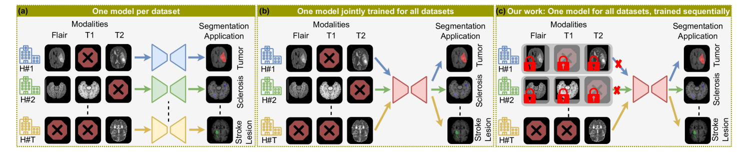
Figure 1: Training paradigms: (a) separate models for fixed modality sets, (b) joint training, and (c) our CL framework enabling sequential training without past data.

This work addresses variable modality MRI segmentation, where datasets arrive sequentially rather than all at once (Fig. 1c). Continual Learning (CL) enables a single model to learn new datasets while retaining past knowledge [McCloskey and Cohen(1989), Ratcliff(1990)]. Naively updating a UNet-based model disrupts previous weights, causing catastrophic forgetting. CL prevents this by using strategies such as storing past data, limiting weight changes, or allocating parameters per dataset. CL is gaining interest in medical image analysis [Kumari et al.(2024)Kumari, Reisenbüchler, Luttner, Schaadt, Feuerhake, and Merhof, Kumari et al.(2023)Kumari, Chauhan, Bozorgpour, Azad, and Merhof] and more specifically also in studies for brain MRI segmentation under domain shifts [Karani et al.(2018)Karani, Chaitanya, Baumgartner, and Konukoglu, van Garderen et al.(2019)van Garderen, van der Voort, Incekara, Smits, and Klein, Baweja et al.(2018)Baweja, Glocker, and Kamnitsas]. However, modality variability remains unexplored. We improve upon [Xu et al.(2024)Xu, Moffat, Seale, Liang, Wagner, Whitehouse, Menon, Newcombe, Voets, Banerjee, et al.] by enabling CL in 3D-UNet without requiring all datasets to be available simultaneously. Our buffer-free approach learns from diverse brain MRI datasets from different hospitals and pathologies. It combines dual-distillation-based regularization with soft parameter isolation for domain adaptation. The dual-distillation method transfers knowledge from the previous model at the feature and response levels to the new model trained on incoming data. Additionally, we integrate mixture-of-experts (MoE) [Shazeer et al.(2017)Shazeer, Mirhoseini, Maziarz, Davis, Le, Hinton, and Dean] within each encoder and decoder layer of UNet to minimize interference between datasets. These experts are activated differently for each data distribution using a domain token, a binary vector encoding modality and pathology information. This targeted activation mechanism helps the model retain knowledge from past datasets more effectively. We summarize our contributions as follows: ❶ To the best of our knowledge, this is the first study exploring CL for brain MRI segmentation under domain shifts, including heterogeneous modalities, pathologies, and acquisition centers. ❷ We introduce a novel domain-conditioned MoE in UNet, incorporating modality and pathology information for 3D segmentation. ❸ Our dual-distillation and MoE-based CL strategy outperforms existing buffer-free CL methods.

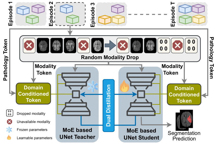
Figure 2: Overview of proposed privacy-aware continual learning framework.

2 Methodology

In CL, a model sequentially learns datasets ($D_{1},D_{2},\dots D_{T}$), each differing in disease type, modalities, and data sources. At any time $t$, only the training set of $D_{t}$ is available, while test sets from all past datasets remain accessible. To prevent catastrophic forgetting without storing past data, we use a buffer-free approach essential for privacy-sensitive applications. Our method employs dual knowledge distillation, where the previous model (teacher, $\mathcal{M}_{t-1}$) guides the current model (student, $\mathcal{M}_{t}$), ensuring knowledge preservation while learning new data. We also integrate a domain-conditioned MoE in convolution layers to minimize interference. The training combines a segmentation loss on the current dataset with dual distillation losses from the teacher model. Additionally, random modality dropout enhances generalization by exposing the model to different modality combinations. A flowchart of our approach is shown in Fig. 2. The next sections detail handling modality variations and our buffer-free CL strategy.

2.1 Variable modality handling

Segmentation datasets in a sequence ($D_{1},D_{2},\dots,D_{T}$) often have distinct MRI modality sets ($N_{1},N_{2},\dots,N_{T}$), where $N_{t}$ represents the modalities available in dataset $D_{t}$. Training with $D_{t}$ requires a UNet with $|{N_{t}}|$ input channels, necessitating a separate UNet for each unique modality set. However, for continual learning across datasets, a single model must handle all modality variations. A simple yet effective solution [Xu et al.(2024)Xu, Moffat, Seale, Liang, Wagner, Whitehouse, Menon, Newcombe, Voets, Banerjee, et al.] uses a single UNet with input channels set to the maximum number of expected modalities $K$, representing possible modalities as ${m_{1},m_{2},\dots,m_{K}}$. This design ensures compatibility with all datasets having $|{N_{t}}|\leq K$. If a modality $m_{k}$ is missing in a dataset, the corresponding channel is zero-filled. To improve generalization and mitigate spurious correlations between datasets and modalities, we employ random modality dropping during training. This exposes the model to varied modality combinations from each dataset, enhancing robustness. While this approach enables handling variable modalities within a unified framework, it is expected to slightly underperform compared to dedicated UNet models tailored for individual datasets.

2.2 Dual distillation

We propose a dual Knowledge Distillation (KD) strategy, transferring knowledge from the teacher to the student model at both latent features and response outputs. This dual alignment preserves structural and contextual information across hierarchies, enhancing the model’s ability to retain learned knowledge. In the response-based KD [Li et al.(2024)Li, Su, Zhang, and Wang], student model is enforced to produce similar output (response) as the teacher model. Typically, KL-divergence between the teacher and student model outputs on current data is used as a regularization term, defined as:

$$\mathcal{L}^{\text{KLD}}=\text{KL}\left(\sigma({\mathcal{M}_{t}(x)}/\tau)||\sigma({\mathcal{M}_{t-1}(x)}/\tau)\right)$$ (1)

where $\text{KL}$ is KL-divergence, $\mathcal{M}_{t}(x)$ and $\mathcal{M}_{t-1}(x)$ are the output logits for input $x$ by $\mathcal{M}_{t}$ and $\mathcal{M}_{t-1}$, $\sigma$ is softmax operator applied to obtain soft targets for KD with temperature $\tau$. Instead of using a static regularization coefficient as in prior works [Li and Hoiem(2018), Kirkpatrick et al.(2017)Kirkpatrick, Pascanu, Rabinowitz, Veness, Desjardins, Rusu, Milan, Quan, Ramalho, Grabska-Barwinska, et al.], we propose a dynamic coefficient ($\alpha_{t}$) for $\mathcal{L}^{\text{KLD}}$, that adapts based on the degree of domain shift between datasets. Greater shifts necessitate stronger regularization to mitigate forgetting. The shift is estimated using the inverse of the Dice Similarity Coefficient (DSC) on unseen data, scaled to a user-defined range $[\alpha_{\text{min}},\alpha_{\text{max}}]$ as $(\alpha_{min}+(1-\text{DSC}^{M_{t-1}}_{D_{t}})(\alpha_{\text{max}}-\alpha_{\text{min}}))$. This dynamic adjustment accounts for variability in dataset distributions, ensuring effective KD.

To complement response-based KD, we add latent-based KD [Li et al.(2024)Li, Su, Zhang, and Wang], which targets the alignment of latent representations between the student and teacher models. To achieve this, we employ a cosine similarity-based regularization loss, $\mathcal{L}^{\text{Cosine}}$, which aligns the latent feature representations of the student model with those of the teacher model

$$\mathcal{L}^{\text{Cosine}}=1-\frac{\mathbf{f}_{\mathcal{M}_{t-1}}\cdot\mathbf{f}_{\mathcal{M}_{t}}}{||\mathbf{f}_{\mathcal{M}_{t-1}}||\,||\mathbf{f}_{\mathcal{M}_{t}}||},$$ (2)

where $\mathbf{f}_{\mathcal{M}_{t-1}}$ and $\mathbf{f}_{\mathcal{M}_{t}}$ represent flattened bottleneck features from the teacher model $\mathcal{M}_{t-1}$ and student model $\mathcal{M}_{t}$, respectively.

2.3 Mixture-of-Expert

When learning a new dataset naively, the model often overwrites previously acquired weights, leading to poor performance on old data. To address dataset conflicts, generic CL literature has mainly explored adding parameter subsets or reserving parameters in fixed networks [De Lange and Tuytelaars(2021)]. However, parameter addition can cause unbounded model growth, while hard reservation restricts knowledge sharing across datasets. To overcome these issues, we draw inspiration from soft parameter reservation techniques in multi-task learning [Shazeer et al.(2017)Shazeer, Mirhoseini, Maziarz, Davis, Le, Hinton, and Dean], which enable flexible capacity sharing across tasks. Specifically, we propose integrating a domain-conditioned MoE mechanism into each convolutional layer of the UNet model. This approach dynamically activates experts with varying strengths based on the domain, achieving soft parameter isolation in a fixed parameter network. The MoE uses a domain-conditioned token derived from dataset-specific metadata to compute gating weights via a linear gating network, $g=\sigma(W_{g}\textbf{c}+b_{g})$, where $\sigma$ is softmax operation, $W_{g}\in\mathbb{R}^{e\times(m+d)}$ and $b_{g}\in\mathbb{R}^{e}$ are the gating network’s parameters for $e$ number of experts, and $\textbf{c}\in\mathbb{R}^{(m+d)}$ is a domain-conditioned token concatenating binary representations of available modalities $\textbf{I}^{m}$ and disease $\textbf{I}^{d}$, with $m$ and $d$ being maximum number of allowed modalities and pathology. This design ensures that each domain is handled uniquely, enabling the model to adaptively allocate expertise. Finally, the gating weights, $g=[g_{1},g_{2},\dots,g_{e}]$, are used to aggregate outputs from $e$ experts, $\{E_{1},E_{2},\dots,E_{e}\}$, as: $y=\sum_{i=1}^{e}g_{i}\cdot E_{i}(f)$, where $f$ is the input feature map, $E_{i}(\cdot)$ is the $i^{th}$ expert, and $y$ is the aggregated output. Unlike hard expert selection, our MoE employs soft selection, allowing contributions from all experts while dynamically adjusting their influence based on the dataset context.

2.4 Model objective

The student model is trained with joint supervision from the teacher model and current data, enabling it to perform effectively on both previously seen and newly introduced data. At any session $t$, the student model $\mathcal{M}_{t}$ is optimized using a total loss $\mathcal{L}^{Total}$, comprising segmentation loss ($\mathcal{L}^{\text{Task}}$), cosine similarity loss ($\mathcal{L}^{Cosine}$), and KL-divergence loss ($\mathcal{L}^{KLD}$). The segmentation loss integrates Dice loss (Dice) and cross-entropy loss (CE), as commonly adopted in literature [Sadegheih et al.(2024)Sadegheih, Bozorgpour, Kumari, Azad, and Merhof]. This multi-component loss enables the model to balance between learning new information and retaining prior knowledge:

$$\mathcal{L}^{\text{Total}}=\underbrace{{\mathcal{L}^{\text{Dice}}+\mathcal{L}^{CE}}}_{\mathcal{L}^{\text{Task}}}+\beta\mathcal{L}^{\text{Cosine}}+\alpha_{t}\mathcal{L}^{KLD}.$$ (3)

Table 1: Dataset details including modalities, pathologies, and number of patients.

Datasets	PD	FLAIR	T1	T1c	T2	DWI	Pathology	#Train patient	#Test patient
BRATS-Decathlon [Bakas et al.(2017)Bakas, Akbari, Sotiras, Bilello, Rozycki, Kirby, Freymann, Farahani, and Davatzikos]	✗	✓	✓	✓	✓	✗	Tumor	444	40
ATLAS V2.0 [Liew et al.(2022)Liew, Lo, Donnelly, Zavaliangos-Petropulu, Jeong, Barisano, Hutton, Simon, Juliano, Suri, et al.]	✗	✗	✓	✗	✗	✗	Stroke lesion	459	196
MSSEG [Commowick et al.(2018)Commowick, Istace, Kain, Laurent, Leray, Simon, Pop, Girard, Ameli, Ferré, et al.]	✓	✓	✓	✓	✓	✗	Sclerosis lesions	37	16
ISLES 2015 [Maier et al.(2017)Maier, Menze, Von der Gablentz, Häni, Heinrich, Liebrand, Winzeck, Basit, Bentley, Chen, et al.]	✗	✓	✓	✗	✓	✓	Stroke lesion	20	8
WMH [Kuijf et al.(2022)Kuijf, Biesbroek, de Bresser, Heinen, Chen, van der Flier, Barkhof, Viergever, and Biessels]	✗	✓	✓	✗	✗	✗	White matter hyperintensity	42	18

3 Experimental setup and results

3.1 Datasets, experimental setup and evaluation metrics

CL experiments are carried out on five brain MRI datasets (BRATS-Decathlon [Bakas et al.(2017)Bakas, Akbari, Sotiras, Bilello, Rozycki, Kirby, Freymann, Farahani, and Davatzikos], MSSEG [Commowick et al.(2018)Commowick, Istace, Kain, Laurent, Leray, Simon, Pop, Girard, Ameli, Ferré, et al.], ATLAS v2.0 [Liew et al.(2022)Liew, Lo, Donnelly, Zavaliangos-Petropulu, Jeong, Barisano, Hutton, Simon, Juliano, Suri, et al.], WMH [Kuijf et al.(2022)Kuijf, Biesbroek, de Bresser, Heinen, Chen, van der Flier, Barkhof, Viergever, and Biessels], ISLES 2015 [Maier et al.(2017)Maier, Menze, Von der Gablentz, Häni, Heinrich, Liebrand, Winzeck, Basit, Bentley, Chen, et al.]) having different modality sets, pathologies, and hospitals, summarized in Table 1. All datasets were skull stripped, resampled to 1x1x1 $mm^{3}$, and z-score normalized per modality. BRATS labels were merged into a single class for binary segmentation, aligning with other datasets.

Our method was implemented using Python 3.10.12 and PyTorch 2.1.0 and trained on an NVIDIA A40 GPU (48 GB VRAM). Each session ran for 400 epochs with a batch size of 4 and an input patch size of 128x128x128. We used the Adam optimizer [Kingma(2014)] (learning rate 0.001, $\beta_{1}=0.9$, and $\beta_{2}=0.999$) without schedulers. Simple random 90-degree rotations were applied for data augmentation, and training across all five datasets took about 20 hours with NVIDIA’s Automatic Mixed Precision (AMP). During the inference phase, we employed MONAI’s [Cardoso et al.(2022)Cardoso, Li, Brown, Ma, Kerfoot, Wang, Murrey, Myronenko, Zhao, Yang, et al.] sliding window technique. Details about the model’s computational demand and complexity are provided in Appendix C.

We compare the proposed strategy against popular CL strategies, including EWC [Kirkpatrick et al.(2017)Kirkpatrick, Pascanu, Rabinowitz, Veness, Desjardins, Rusu, Milan, Quan, Ramalho, Grabska-Barwinska, et al.], SI [Zenke et al.(2017)Zenke, Poole, and Ganguli], LwF [Li and Hoiem(2018)], MiB [Cermelli et al.(2020)Cermelli, Mancini, Bulo, Ricci, and Caputo], Replay [Rolnick et al.(2019)Rolnick, Ahuja, Schwarz, Lillicrap, and Wayne], and GDumb [Prabhu et al.(2020)Prabhu, Torr, and Dokania] in 3D-UNet. To establish baselines, we report lower bound performance with naive, and upper bounds with cumulative and joint training. Naive corresponds to traditional fine-tuning on new datasets, joint training uses all datasets simultaneously, and cumulative training sequentially incorporates all previous data. Experiments were conducted using Avalanche 0.6.0 framework [Lomonaco et al.(2021)Lomonaco, Pellegrini, Cossu, Carta, Graffieti, Hayes, Lange, Masana, Pomponi, van de Ven, Mundt, She, Cooper, Forest, Belouadah, Calderara, Parisi, Cuzzolin, Tolias, Scardapane, Antiga, Amhad, Popescu, Kanan, van de Weijer, Tuytelaars, Bacciu, and Maltoni]. The buffer size was set to $200$ for Replay and GDumb. Regularization factors ($\alpha$ in LwF and $\lambda$ in SI and EWC) were tuned within 0.5, 1.0, 1.5, 2.0, and $\tau$ was fixed at $2$. For our method, we set $\beta=0.8$, $\alpha_{max}=0.6$, and $e=4$. For domain-conditioned MoE, we consider maximum modalities as $m=6$ (PD, FLAIR, T1, T1c, T2, DWI) and pathology as $d=4$ (Tumor, Stroke lesion, Sclerosis lesions, White matter hyperintensity). An example of the binary domain-conditioned token ($\textbf{I}^{d+m}$) for a sample with FLAIR and T1 modality and “stroke lesion” pathology would be [0, 1, 1, 0, 0, 0, 0, 1, 0, 0]. We tested on four dataset sequences: S1 (high to low dataset size: {BRATS, ATLAS, MSSEG, ISLES, WMH}), S2 (descending modality count: {MSSEG, BRATS, ISLES, WMH, ATLAS}), S3 (low to high dataset size: {ISLES, WMH, MSSEG, BRATS, ATLAS}), and S4 (ascending modality count: {ATLAS, WMH, ISLES, BRATS, MSSEG}).

In CL with five datasets, training occurs sequentially across five sessions, with the model evaluation after each session on the test sets of all datasets. Consequently, for $P$ datasets, this process generates a $(P\times P)$ train-test matrix, where each cell $p_{ij}$ indicates the DSC on the test set of $D_{j}$ after sequential training from $D_{1}$ to $D_{i}$. CL-specific metrics including backward transfer (BWT) [Díaz-Rodríguez et al.(2018)Díaz-Rodríguez, Lomonaco, Filliat, and Maltoni] and forward transfer (FWT) [Özgün et al.(2020)Özgün, Rickmann, Roy, and Wachinger] are derived from this matrix. We also report average performance (ACC), which measures DSC across all datasets after the $P^{th}$ session [Lopez-Paz and Ranzato(2017)], and the Incremental Learning Metric (ILM), i.e. the average of cells in the lower triangle of the matrix including diagonals, reflecting incremental learning capability [Díaz-Rodríguez et al.(2018)Díaz-Rodríguez, Lomonaco, Filliat, and Maltoni]. Higher values of BWT, FWT, ACC, and ILM indicate better performance.

Table 2: Performance comparison (best, second best result in buffer-free CL). $\mathcal{B}$ = buffer.

			S1				S2
$\mathcal{B}$	Method	Hyper- parameter	ACC$\uparrow$	ILM$\uparrow$	BWT$\uparrow$	FWT$\uparrow$	ACC$\uparrow$	ILM$\uparrow$	BWT$\uparrow$	FWT$\uparrow$
✓	Joint		67.62	-	-	-	67.96	-	-	-
	Cumulative		62.37	67.40	-1.60	29.83	69.2	73.04	0.05	21.46
	GDumb	mem=200	50.43	58.74	-1.33	28.27	50.63	62.42	-11.89	21.25
	Replay	mem=200	67.09	68.62	-4.98	33.08	70.83	74.36	-0.33	22.59
✗	Naive		15.73	33.64	-54.14	22.37	23.43	37.36	-54.16	17.94
	MiB		26.89	41.80	-45.06	23.52	24.39	38.35	-53.03	23.22
	LwF	$\alpha$=0.5	17.77	33.24	-56.68	19.93	15.92	35.60	-54.69	19.02
		$\alpha$=1	29.97	41.18	-45.15	22.37	18.16	36.05	-57.54	21.18
		$\alpha$=1.5	24.52	35.60	-52.18	18.67	18.00	32.48	-58.61	17.14
		$\alpha$=2	19.50	35.16	-54.17	21.90	12.46	34.97	-57.32	18.88
	SI	$\lambda$=0.5	37.45	48.28	-32.78	28.45	13.32	36.83	-52.69	18.00
		$\lambda$=1	36.94	49.39	-27.84	29.93	13.57	33.20	-57.45	17.60
		$\lambda$=1.5	25.02	42.01	-36.64	29.65	7.78	34.03	-50.27	18.95
		$\lambda$=2	43.27	51.69	-25.07	31.31	12.38	35.00	-54.06	16.69
	EWC	$\lambda$=0.5	21.46	33.66	-55.31	20.32	22.11	36.60	-54.53	19.32
		$\lambda$=1	26.48	39.04	-45.30	21.05	26.78	39.84	-52.89	20.15
		$\lambda$=1.5	18.18	34.71	-56.52	25.41	16.97	35.02	-59.57	21.61
		$\lambda$=2	22.18	36.17	-50.75	19.84	22.88	36.16	-51.59	18.77
	Proposed		54.31	56.46	-16.46	30.73	28.54	49.91	-34.26	23.93
			S3				S4
✓	Joint		66.93	-	-	-	64.36	-	-	-
	Cumulative		67.12	67.54	-0.09	24.31	66.79	61.04	-1.33	16.31
	GDumb	mem=200	56.63	63.00	-1.59	22.35	58.10	52.69	-5.42	17.14
	Replay	mem=200	70.68	66.79	3.93	19.71	65.68	63.03	1.11	8.15
✗	Naive		24.78	39.49	-41.01	12.06	36.66	39.58	-38.69	14.73
	MiB		31.28	39.37	-39.83	12.15	39.47	39.43	-35.96	18.57
	LwF	$\alpha$=0.5	24.82	38.24	-40.10	14.31	35.42	38.05	-37.83	14.08
		$\alpha$=1	23.73	35.68	-38.99	14.23	33.40	38.29	-38.66	17.59
		$\alpha$=1.5	23.06	36.72	-47.43	15.06	39.71	39.68	-38.10	15.70
		$\alpha$=2	24.36	38.48	-48.30	14.71	36.90	39.01	-38.47	14.84
	SI	$\lambda$=0.5	31.57	41.16	-37.79	15.56	36.27	38.66	-36.39	20.80
		$\lambda$=1	18.93	35.72	-46.10	11.16	47.06	43.87	-25.94	13.68
		$\lambda$=1.5	24.27	39.04	-35.24	13.82	44.30	40.01	-27.06	13.82
		$\lambda$=2	20.62	41.02	-40.27	25.05	43.12	41.81	-27.01	18.16
	EWC	$\lambda$=0.5	34.19	41.55	-37.65	13.97	39.93	40.06	-34.97	14.37
		$\lambda$=1	15.51	33.83	-45.89	13.46	27.84	35.86	-40.57	13.31
		$\lambda$=1.5	19.68	38.05	-42.49	13.03	37.90	39.05	-36.33	13.61
		$\lambda$=2	24.69	38.91	-43.03	17.91	33.99	37.35	-34.61	13.81
	Proposed		35.85	46.13	-21.09	21.53	50.67	48.54	-21.37	16.00

3.2 Results and discussion

Performance comparison with others: For the considered medical applications, the primary concern will not be on improving zero-shot performance (FWT) but rather on minimizing forgetting (BWT) and enhancing the average DSC of the model (ACC and ILM). While FWT is reported for completeness, our analysis emphasize ACC, ILM, and BWT. Table 2 presents the ACC, ILM, BWT, and FWT values for all methods across sequences S1, S2, S3, and S4. Across all sequences, CL approaches (GDumb, Replay, MiB, LwF, SI, EWC, and the proposed method) mostly outperform naive training, highlighting the importance of mechanisms to mitigate catastrophic forgetting in UNet-based segmentation tasks. Further, as expected, approaches storing past data partially (Replay, GDumb) or fully (cumulative, joint training) show higher performance compared to methods (naive, MiB, LwF, SI, EWC, and the proposed approach) with no access to past exemplars. When comparing the proposed method to other buffer-free approaches (MiB, LwF, SI, EWC), it consistently achieves superior performance in all the sequences S1, S2, S3, and S4. Unlike these existing CL methods, which penalize large deviations from previously learned weights through response-level regularization terms in the training loss, the proposed approach introduces a drift-based dynamic penalization factor along with a latent-level regularization. This drift-based dual distillation allows for more effective mitigation of catastrophic forgetting. The proposed method shows a positive gain in (ACC, ILM, BWT) over best performance achieved among state-of-the art buffer-free approaches (blue colored in Table 2). Specifically, we observe an improvements of (25.51%, 9.23%, 34.34%) in S1, (6.57%, 25.28%, 31.85%) in S2, (4.85%, 11.02%, 40.15%) in S3, and (7.67%, 10.65%, 17.62%) in S4. For intuitive visualization, radar plots for S1, S2, S3, and S4, comparing cumulative, naive, the best-performing buffer-free methods, and the proposed approach are provided in Fig. 6 of Appendix.

Performance of a dataset in different sessions: We closely analyze CL model’s performances on first/second dataset upon learning other datasets in a given sequence. Specifically, Figure 3 shows DSC for BRATS in S1 and S2, ISLES in S3, and WMH in S4, with cumulative training included for reference. While cumulative training offers stable results, it requires access to all previous datasets, which is impractical in real-world scenarios. The naive approach shows significant DSC degradation, with high standard deviations of 33.91 (S1) and 40.23 (S2), 26.31 (S3), and 24.78 (S4) reflecting instability. In contrast, our CL strategy maintains stability, with much lower standard deviations of 5.19 (S1), 14.51 (S2), 11.37 (S3), and 15.50 (S4) highlighting its increased robustness against forgetting. Other buffer-free CL methods (MiB, SI, EWC, LwF) show better performance than naive training (Table 2) but still exhibit instability in DSC, with standard deviations of (28.80, 17.86, 31.14, 25.98) for S1, (36.75, 36.75, 35.85, 40.10) for S2, (25.43, 23.51, 25.65, 25.11) for S3, and (25.06, 15.51, 22.84, 23.55) for S4. While these methods perform well for natural images, their effectiveness is limited in brain MRI segmentation under domain shifts. In contrast, our approach delivers better stability and mitigates catastrophic forgetting effectively. Detailed segmentation visualizations for BRATS are provided in Appendix A.

Impact of dataset orders: We study the impact of different sequences on overall performance. We analyze ACC, ILM, BWT by best performing other CL methods and proposed approach for S1-S4 in Table 2 (summarized in Table 4, Appendix). We can see that best ACC is poor in S2 (28.54) and S3 (35.85) as compared to that in S1 (54.31) and S4 (50.67). Notably, all methods (except EWC) showed performance degradation when ATLAS (a single-modality dataset) was introduced later in sequences (S2, S3), adversely impacting the generalization of previously acquired knowledge in the model. This occurs because “modality dropping”, a critical generalization technique, cannot be applied to ATLAS due to its single-modality nature. Consequently, learning ATLAS in the later stages negatively impacts the model’s prior generalization capability. In contrast, when we learn datasets with fewer modalities at the start of sequences (S1 and S4), their negative effect is covered at later stages when we learn datasets with more modalities.

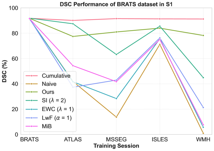
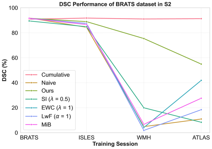
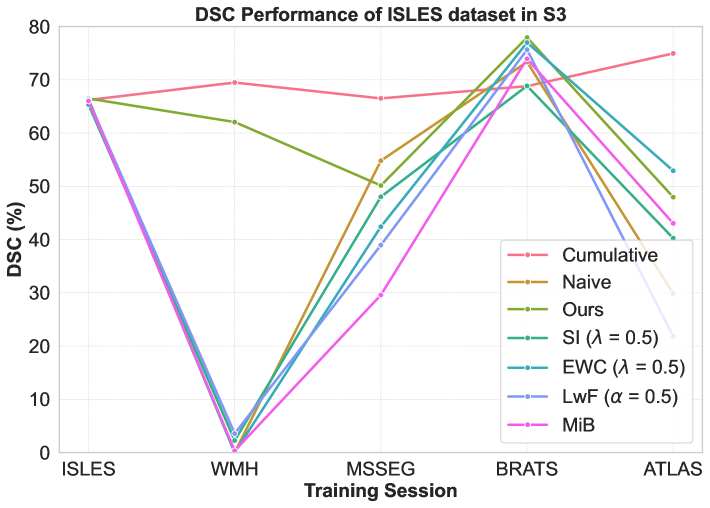
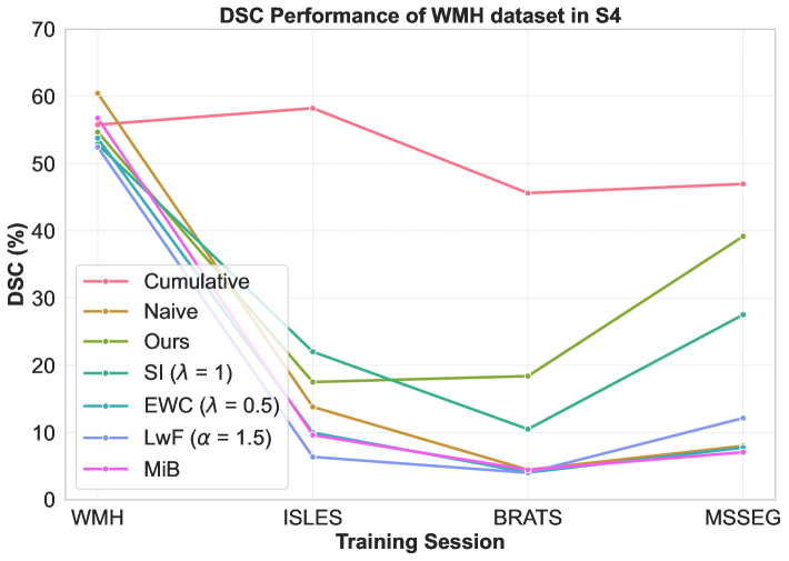
Figure 3: DSC on already learned datasets upon learning new datasets in different sequences

3.3 Ablation study

We present the results of our ablation study in Table 3, showing that all modules of our approach, both individually and in combination, outperform naive UNet training for variable-modality brain MRI segmentation. Notably, our dynamic regularization coefficient for response-based regularization ($\mathcal{L}^{\text{KLD}}$) outperforms the static coefficient in LwF (Table 2). While LwF achieves ILM scores of 41.18 and 36.05 in S1 and S2, respectively, our dynamic setting results in higher ILM scores of 47.16 and 38.81. This approach not only improves performance but also eliminates the need to manually select suitable $\alpha$ for a given dataset sequence. We also observe that removing the random dropping of modalities harms performance, as the model learns undesired association of a dataset with a fixed modality set, preventing it from developing generalized representations, which are crucial for learning diverse datasets within a single model. Next, we analyze the contribution of each module in our approach. In S1, response-based regularization outperforms latent-based regularization, while the reverse is true in S2. However, their combination, the dual-distillation consistently outperforms both in S1 and S2, supporting its inclusion in the proposed strategy. Additionally, the domain-conditioned MoE ($\textbf{I}^{d+m}$) outperforms naive UNet in both experiments. Studying the joint token ($\textbf{I}^{d+m}$) against the individual modality-only ($\textbf{I}^{m}$) and disease-only ($\textbf{I}^{d}$) tokens in presence or absence of dual distillation, we find that their combination outperforms the individual tokens. Further, when the joint token is combined with dual-distillation, average DSC improves significantly: ILM increases from 52.03 to 56.46 in S1 and from 45.58 to 49.91 in S2, reflecting gains of 8.51% and 9.50%, respectively. These results demonstrate the complementary benefits of dual-distillation and domain-conditioned MoE, highlighting the effectiveness of our hybrid CL strategy.

Table 3: Ablation study. Bold refers to proposed approach.

				S1				S2
Method	$\mathcal{L}^{\text{KLD}}$	$\mathcal{L}^{\text{Cosine}}$	MoE	ACC$\uparrow$	ILM$\uparrow$	BWT$\uparrow$	FWT$\uparrow$	ACC$\uparrow$	ILM$\uparrow$	BWT$\uparrow$	FWT $\uparrow$
Naive	-	-	-	15.73	33.64	-54.14	22.37	23.43	37.36	-54.16	17.94
	✓	✗	✗	41.29	47.16	-11.31	24.37	13.79	38.81	-30.43	23.13
	✗	✓	✗	24.31	37.85	-51.90	25.66	33.23	42.25	-48.39	25.44
	✓	✓	✗	49.20	52.03	-18.82	32.34	29.62	45.58	-15.89	22.38
	✗	✗	$\textbf{I}^{d}$	20.21	35.32	-56.74	22.22	25.05	37.88	-56.01	23.17
Our	✗	✗	$\textbf{I}^{m}$	22.19	38.59	-51.06	25.23	21.50	38.13	-55.61	21.27
	✗	✗	$\textbf{I}^{d+m}$	22.91	42.36	-45.83	25.65	23.13	41.40	-51.21	26.09
	✓	✓	$\textbf{I}^{d}$	47.29	54.94	-20.59	29.63	26.76	48.92	-35.68	22.14
	✓	✓	$\textbf{I}^{m}$	40.28	48.55	-33.07	21.10	13.17	44.32	-40.23	24.71
	✓	✓	$\textbf{I}^{d+m}$	54.31	56.46	-16.46	30.73	28.54	49.91	-34.26	23.93
Without modality drop strategy				34.80	37.65	-50.15	13.41	18.25	35.08	-58.58	15.92

3.4 Limitations and future work

This work takes an initial step toward buffer-free CL for brain lesion segmentation across variable modalities with a simple training setup. While it outperforms naive training and other CL strategies, some limitations remain. Its performance still lags behind models trained separately for each dataset or modality set, highlighting the trade-offs of a unified CL model. Enhanced training setups, such as extended schedules or hyperparameter tuning, could improve results. Additionally, while avoiding a buffer is practical, it may negatively impact long-term retention and increase catastrophic forgetting when dealing with highly diverse datasets. Future work will explore privacy-preserving latent data generators as a proxy for replay methods and focus on adaptive learning schedules, optimized architectures, and expansion to larger datasets, modalities, and real-world clinical settings.

4 Conclusion

This work tackles brain lesion segmentation in multi-modal MRI under real-world constraints, where datasets arrive sequentially with varying modalities. We introduced a hybrid continual learning strategy that enables a single segmentation model to learn from diverse datasets without requiring all data at once. Using two-stage distillation and a mixture-of-experts mechanism, our approach reduces catastrophic forgetting while preserving performance on previously seen data. Experiments on five diverse brain MRI datasets in four different sequences validate its effectiveness in handling variations across modalities, hospitals, and pathologies. This study marks a step toward practical, scalable multi-modal MRI segmentation, demonstrating the potential of continual learning in neuroimage analysis.

asdCumulative
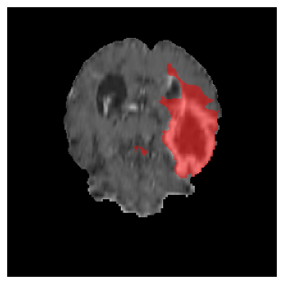
asdqwNaive
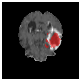
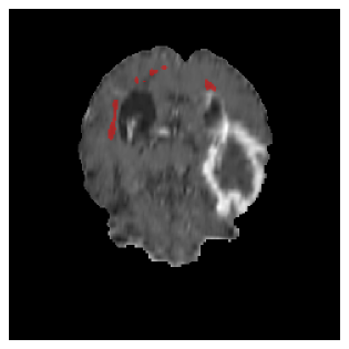
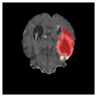
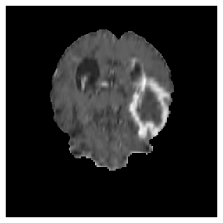
assdadOurs
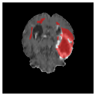
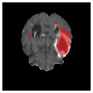
assddSI ($\lambda=2$)
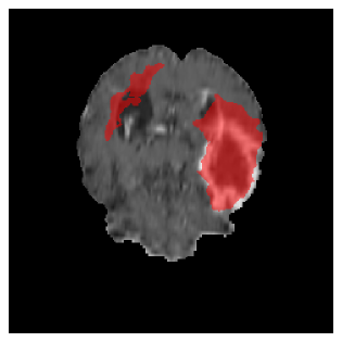
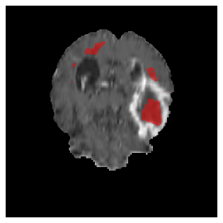
	Ground Truth	Episode 1	Episode 2	Episode 3	Episode 4	Episode 5

Figure 4: Qualitative comparison of a patient in BRATS dataset during different episodes with different methodology in S1.

asdCumulative
asdqwNaive
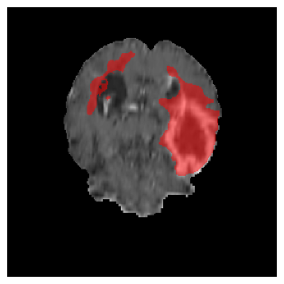
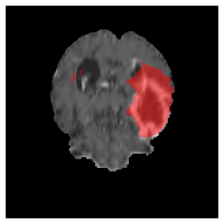
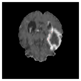
assdadOurs
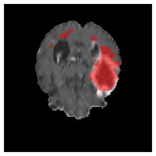
asEWC ($\lambda=1$)
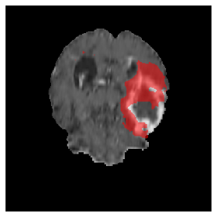
	Ground Truth	Episode 2	Episode 3	Episode 4	Episode 5

Figure 5: Qualitative comparison of a patient in BRATS dataset during different episodes with different methodology in S2.

Appendix A Qualitative results

Figures 4 and 5 present the segmentation results for a patient from the BRATS dataset, visualized on a randomly selected slice. Figure 4 illustrates how tumor segmentation evolves over multiple episodes in S1 across different approaches including cumulative, naive, our approach, and the best buffer-free strategy (SI, $\lambda$=2). The cumulative approach, which trains on all encountered datasets together, maintains segmentation consistency across episodes but introduces significant amounts of false positives, particularly in the upper left area of the brain images. These misclassifications highlight its inability to generalize well across datasets despite access to all previous data. The naive approach, which learns sequentially without any continual learning strategy, suffers from severe catastrophic forgetting. While it initially segments well, performance deteriorates over episodes, leading to a near-complete loss of segmentation capability by the final episode. The SI ($\lambda$=2) approach, a regularization-based buffer-free CL strategy, performs reasonably well in early episodes but shows a significant performance decline over time. By the last episode, much of the tumor was no longer segmented, indicating difficulty in retaining prior knowledge. In contrast, our proposed approach initially produces more false positives but progressively refines its segmentation. By the final episode, it accurately retains the tumor region while minimizing misclassifications, demonstrating strong knowledge retention and adaptability across episodes. This suggests that our approach effectively mitigates catastrophic forgetting while maintaining segmentation performance over sequential learning.

Figure 5 illustrates the segmentation evolution for the same BRATS patient in S2 sequence. The key difference here is that the best buffer-free strategy is EWC ($\lambda$=1), and training on BRATS data starts from episode 2 instead of episode 1 as BRATS is encountered at episode 2 in S2. The cumulative approach retains segmentation across episodes but continues to generate false positives, which become even more pronounced in the final episode. The naive approach, lacking a CL mechanisms, completely overrides previous knowledge, leading to failed segmentation in later episodes. EWC ($\lambda$=1) approach initially maintains segmentation but experiences a sharp decline in episode 4, where it fails to segment the tumor. In the final episode, it undersegments the lesion, missing a significant portion of the tumor. In contrast, the proposed approach consistently preserves segmentation across episodes. While initially introducing false positives, it gradually refines predictions, retaining the tumor region while minimizing misclassifications. It maintains clear tumor delineation by the final episode, demonstrating effective knowledge retention and adaptability throughout training.

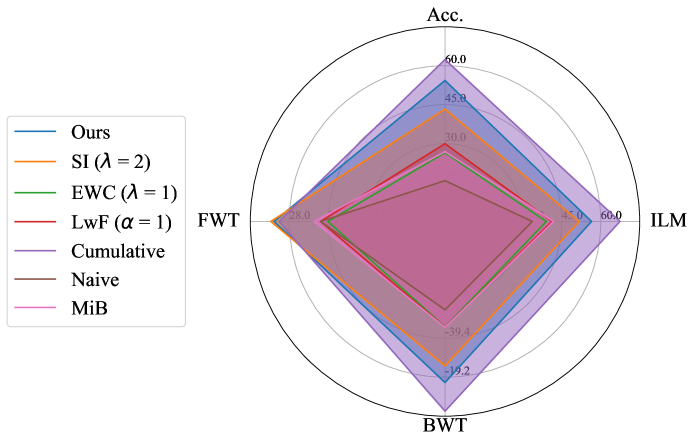
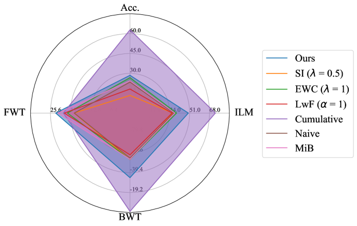
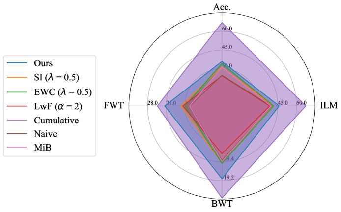
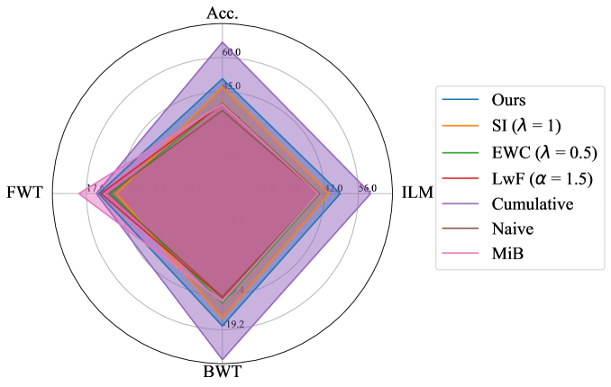
Figure 6: Comparison with best results by MiB, SI, EWC, and LwF. First row: left (S1) and right (S2) and second row: left (S3) and right (S4).

Appendix B Radar Plot based Comparison

For intuitive visualization, Fig. 6 provides a radar plot comparing cumulative, naive, the best-performing buffer-free CL methods, and the proposed approach. In all the formulated dataset sequences, the proposed method demonstrates clear superiority over all other approaches except cumulative, which serves as the upper performance bound.

Table 4: Sequences analysis for different CL approaches.

	S1			S2			S3			S4
Method	ACC$\uparrow$	ILM$\uparrow$	BWT$\uparrow$	ACC$\uparrow$	ILM$\uparrow$	BWT$\uparrow$	ACC$\uparrow$	ILM$\uparrow$	BWT$\uparrow$	ACC$\uparrow$	ILM$\uparrow$	BWT$\uparrow$
MiB	26.89	41.80	-45.06	24.39	38.35	-53.03	31.28	39.37	-39.83	39.47	39.43	-35.96
LwF	29.97	41.18	-45.15	18.16	36.05	-57.54	24.82	38.24	-40.10	39.71	39.68	-38.10
SI	43.27	51.69	-25.07	13.32	36.83	-52.69	31.57	41.16	-37.79	47.06	43.87	-25.94
EWC	26.48	39.04	-45.30	26.78	39.84	-52.89	34.19	41.55	-37.65	39.93	40.06	-34.97
Proposed	54.31	56.46	-16.46	28.54	49.91	-34.26	35.85	46.13	-21.09	50.67	48.54	-21.37

Appendix C Computational Details

The baseline vanilla 3D UNet, configured with six input channels (corresponding to different MRI modalities) and two output channels (background and lesion), has approximately 8.9 million parameters and requires approximately 139.83 GFLOPS per inference for an input size of 128×128×128. By integrating the Mixture-of-Experts (MoE) mechanism, our proposed model slightly increases in complexity, featuring approximately 18.38M parameters and requiring around 195.46 GFLOPS. This additional complexity arises due to the inclusion of four experts per convolutional layer and the associated soft-selection mechanism based on a 10-dimensional domain-conditioned context vector. Moreover, while our dual-distillation approach temporarily doubles the inference computation during training, the deployed model involves a single network inference at test time, ensuring practical computational efficiency suitable for clinical scenarios. Our proposed approach maintains a practical balance between performance and computational cost, emphasizing its feasibility and applicability for real-world clinical deployment.

References

- [Bakas et al.(2017)Bakas, Akbari, Sotiras, Bilello, Rozycki, Kirby, Freymann, Farahani, and Davatzikos] Spyridon Bakas, Hamed Akbari, Aristeidis Sotiras, Michel Bilello, Martin Rozycki, Justin S Kirby, John B Freymann, Keyvan Farahani, and Christos Davatzikos. Advancing the cancer genome atlas glioma mri collections with expert segmentation labels and radiomic features. Scientific data, 4(1):1–13, 2017.
- [Baweja et al.(2018)Baweja, Glocker, and Kamnitsas] Chaitanya Baweja, Ben Glocker, and Konstantinos Kamnitsas. Towards continual learning in medical imaging. arXiv preprint arXiv:1811.02496, 2018.
- [Cardoso et al.(2022)Cardoso, Li, Brown, Ma, Kerfoot, Wang, Murrey, Myronenko, Zhao, Yang, et al.] M Jorge Cardoso, Wenqi Li, Richard Brown, Nic Ma, Eric Kerfoot, Yiheng Wang, Benjamin Murrey, Andriy Myronenko, Can Zhao, Dong Yang, et al. Monai: An open-source framework for deep learning in healthcare. arXiv preprint arXiv:2211.02701, 2022.
- [Cermelli et al.(2020)Cermelli, Mancini, Bulo, Ricci, and Caputo] Fabio Cermelli, Massimiliano Mancini, Samuel Rota Bulo, Elisa Ricci, and Barbara Caputo. Modeling the background for incremental learning in semantic segmentation. In Proceedings of the IEEE/CVF Conference on Computer Vision and Pattern Recognition, pages 9233–9242, 2020.
- [Commowick et al.(2018)Commowick, Istace, Kain, Laurent, Leray, Simon, Pop, Girard, Ameli, Ferré, et al.] Olivier Commowick, Audrey Istace, Michael Kain, Baptiste Laurent, Florent Leray, Mathieu Simon, Sorina Camarasu Pop, Pascal Girard, Roxana Ameli, Jean-Christophe Ferré, et al. Objective evaluation of multiple sclerosis lesion segmentation using a data management and processing infrastructure. Scientific reports, 8(1):13650, 2018.
- [De Lange and Tuytelaars(2021)] Matthias De Lange and Tinne Tuytelaars. Continual prototype evolution: Learning online from non-stationary data streams. In Proceedings of the IEEE/CVF international conference on computer vision, pages 8250–8259, 2021.
- [Díaz-Rodríguez et al.(2018)Díaz-Rodríguez, Lomonaco, Filliat, and Maltoni] Natalia Díaz-Rodríguez, Vincenzo Lomonaco, David Filliat, and Davide Maltoni. Don’t forget, there is more than forgetting: new metrics for continual learning. arXiv preprint arXiv:1810.13166, 2018.
- [Karani et al.(2018)Karani, Chaitanya, Baumgartner, and Konukoglu] Neerav Karani, Krishna Chaitanya, Christian Baumgartner, and Ender Konukoglu. A lifelong learning approach to brain mr segmentation across scanners and protocols. In International conference on medical image computing and computer-assisted intervention, pages 476–484. Springer, 2018.
- [Kingma(2014)] Diederik P Kingma. Adam: A method for stochastic optimization. arXiv preprint arXiv:1412.6980, 2014.
- [Kirkpatrick et al.(2017)Kirkpatrick, Pascanu, Rabinowitz, Veness, Desjardins, Rusu, Milan, Quan, Ramalho, Grabska-Barwinska, et al.] James Kirkpatrick, Razvan Pascanu, Neil Rabinowitz, Joel Veness, Guillaume Desjardins, Andrei A Rusu, Kieran Milan, John Quan, Tiago Ramalho, Agnieszka Grabska-Barwinska, et al. Overcoming catastrophic forgetting in neural networks. Proceedings of the national academy of sciences, 114(13):3521–3526, 2017.
- [Kuijf et al.(2022)Kuijf, Biesbroek, de Bresser, Heinen, Chen, van der Flier, Barkhof, Viergever, and Biessels] Hugo Kuijf, Matthijs Biesbroek, Jeroen de Bresser, Rutger Heinen, Christopher Chen, Wiesje van der Flier, Barkhof, Max Viergever, and Geert Jan Biessels. Data of the White Matter Hyperintensity (WMH) Segmentation Challenge, 2022. URL https://doi.org/10.34894/AECRSD.
- [Kumari et al.(2023)Kumari, Chauhan, Bozorgpour, Azad, and Merhof] Pratibha Kumari, Joohi Chauhan, Afshin Bozorgpour, Reza Azad, and Dorit Merhof. Continual learning in medical imaging analysis: A comprehensive review of recent advancements and future prospects. arXiv preprint arXiv:2312.17004, 2023.
- [Kumari et al.(2024)Kumari, Reisenbüchler, Luttner, Schaadt, Feuerhake, and Merhof] Pratibha Kumari, Daniel Reisenbüchler, Lucas Luttner, Nadine S Schaadt, Friedrich Feuerhake, and Dorit Merhof. Continual domain incremental learning for privacy-aware digital pathology. In International Conference on Medical Image Computing and Computer-Assisted Intervention, pages 34–44. Springer, 2024.
- [Li et al.(2024)Li, Su, Zhang, and Wang] Songze Li, Tonghua Su, Xuyao Zhang, and Zhongjie Wang. Continual learning with knowledge distillation: A survey. Authorea Preprints, 2024.
- [Li and Hoiem(2018)] Zhizhong Li and Derek Hoiem. Learning without forgetting. IEEE Transactions on Pattern Analysis and Machine Intelligence, 40(12):2935–2947, 2018. 10.1109/TPAMI.2017.2773081.
- [Liew et al.(2022)Liew, Lo, Donnelly, Zavaliangos-Petropulu, Jeong, Barisano, Hutton, Simon, Juliano, Suri, et al.] Sook-Lei Liew, Bethany P Lo, Miranda R Donnelly, Artemis Zavaliangos-Petropulu, Jessica N Jeong, Giuseppe Barisano, Alexandre Hutton, Julia P Simon, Julia M Juliano, Anisha Suri, et al. A large, curated, open-source stroke neuroimaging dataset to improve lesion segmentation algorithms. Scientific data, 9(1):320, 2022.
- [Lomonaco et al.(2021)Lomonaco, Pellegrini, Cossu, Carta, Graffieti, Hayes, Lange, Masana, Pomponi, van de Ven, Mundt, She, Cooper, Forest, Belouadah, Calderara, Parisi, Cuzzolin, Tolias, Scardapane, Antiga, Amhad, Popescu, Kanan, van de Weijer, Tuytelaars, Bacciu, and Maltoni] Vincenzo Lomonaco, Lorenzo Pellegrini, Andrea Cossu, Antonio Carta, Gabriele Graffieti, Tyler L. Hayes, Matthias De Lange, Marc Masana, Jary Pomponi, Gido van de Ven, Martin Mundt, Qi She, Keiland Cooper, Jeremy Forest, Eden Belouadah, Simone Calderara, German I. Parisi, Fabio Cuzzolin, Andreas Tolias, Simone Scardapane, Luca Antiga, Subutai Amhad, Adrian Popescu, Christopher Kanan, Joost van de Weijer, Tinne Tuytelaars, Davide Bacciu, and Davide Maltoni. Avalanche: an end-to-end library for continual learning. In Proceedings of IEEE Conference on Computer Vision and Pattern Recognition, 2nd Continual Learning in Computer Vision Workshop, 2021.
- [Lopez-Paz and Ranzato(2017)] David Lopez-Paz and Marc’Aurelio Ranzato. Gradient episodic memory for continual learning. Advances in neural information processing systems, 30, 2017.
- [Maier et al.(2017)Maier, Menze, Von der Gablentz, Häni, Heinrich, Liebrand, Winzeck, Basit, Bentley, Chen, et al.] Oskar Maier, Bjoern H Menze, Janina Von der Gablentz, Levin Häni, Mattias P Heinrich, Matthias Liebrand, Stefan Winzeck, Abdul Basit, Paul Bentley, Liang Chen, et al. Isles 2015-a public evaluation benchmark for ischemic stroke lesion segmentation from multispectral mri. Medical image analysis, 35:250–269, 2017.
- [McCloskey and Cohen(1989)] Michael McCloskey and Neal J Cohen. Catastrophic interference in connectionist networks: The sequential learning problem. In Psychology of learning and motivation, volume 24, pages 109–165. Elsevier, 1989.
- [Özgün et al.(2020)Özgün, Rickmann, Roy, and Wachinger] Sinan Özgün, Anne-Marie Rickmann, Abhijit Guha Roy, and Christian Wachinger. Importance driven continual learning for segmentation across domains. In Machine Learning in Medical Imaging: 11th International Workshop, MLMI 2020, Held in Conjunction with MICCAI 2020, Lima, Peru, October 4, 2020, Proceedings 11, pages 423–433. Springer, 2020.
- [Prabhu et al.(2020)Prabhu, Torr, and Dokania] Ameya Prabhu, Philip HS Torr, and Puneet K Dokania. Gdumb: A simple approach that questions our progress in continual learning. In Computer Vision–ECCV 2020: 16th European Conference, Glasgow, UK, August 23–28, 2020, Proceedings, Part II 16, pages 524–540. Springer, 2020.
- [Ratcliff(1990)] Roger Ratcliff. Connectionist models of recognition memory: constraints imposed by learning and forgetting functions. Psychological review, 97(2):285, 1990.
- [Rolnick et al.(2019)Rolnick, Ahuja, Schwarz, Lillicrap, and Wayne] David Rolnick, Arun Ahuja, Jonathan Schwarz, Timothy Lillicrap, and Gregory Wayne. Experience replay for continual learning. Advances in Neural Information Processing Systems, 32, 2019.
- [Sadegheih et al.(2024)Sadegheih, Bozorgpour, Kumari, Azad, and Merhof] Yousef Sadegheih, Afshin Bozorgpour, Pratibha Kumari, Reza Azad, and Dorit Merhof. Lhu-net: A light hybrid u-net for cost-efficient, high-performance volumetric medical image segmentation. arXiv preprint arXiv:2404.05102, 2024.
- [Shazeer et al.(2017)Shazeer, Mirhoseini, Maziarz, Davis, Le, Hinton, and Dean] Noam Shazeer, Azalia Mirhoseini, Krzysztof Maziarz, Andy Davis, Quoc Le, Geoffrey Hinton, and Jeff Dean. Outrageously large neural networks: The sparsely-gated mixture-of-experts layer. arXiv preprint arXiv:1701.06538, 2017.
- [van Garderen et al.(2019)van Garderen, van der Voort, Incekara, Smits, and Klein] Karin van Garderen, Sebastian van der Voort, Fatih Incekara, Marion Smits, and Stefan Klein. Towards continuous learning for glioma segmentation with elastic weight consolidation. arXiv preprint arXiv:1909.11479, 2019.
- [Wagner et al.(2024)Wagner, Xu, Saha, Liang, Whitehouse, Menon, Voets, Noble, and Kamnitsas] Felix Wagner, Wentian Xu, Pramit Saha, Ziyun Liang, Daniel Whitehouse, David Menon, Natalie Voets, J Alison Noble, and Konstantinos Kamnitsas. Feasibility of federated learning from client databases with different brain diseases and mri modalities. arXiv preprint arXiv:2406.11636, 2024.
- [Xu et al.(2024)Xu, Moffat, Seale, Liang, Wagner, Whitehouse, Menon, Newcombe, Voets, Banerjee, et al.] Wentian Xu, Matthew Moffat, Thalia Seale, Ziyun Liang, Felix Wagner, Daniel Whitehouse, David Menon, Virginia Newcombe, Natalie Voets, Abhirup Banerjee, et al. Feasibility and benefits of joint learning from mri databases with different brain diseases and modalities for segmentation. arXiv preprint arXiv:2405.18511, 2024.
- [Zenke et al.(2017)Zenke, Poole, and Ganguli] Friedemann Zenke, Ben Poole, and Surya Ganguli. Continual learning through synaptic intelligence. In International conference on machine learning, pages 3987–3995. PMLR, 2017.