Structure Identification of NDS with Descriptor Subsystems under Asynchronous, Non-Uniform, and Slow-Rate Sampling

Abstract

Networked dynamic systems (NDS) exhibit collective behavior shaped by subsystem dynamics and complex interconnections, yet identifying these interconnections remains challenging due to irregularities in sampled data, including asynchronous, non-uniform, and low-rate sampling. This paper proposes a novel two-stage structure identification algorithm that leverages system zero-order moments, a concept traditionally used in model order reduction, to bridge system identification and model reduction. First, zero-order moments are estimated from steady-state time-domain outputs; second, subsystem interconnections are explicitly reconstructed from these moments. The method generalizes existing approaches by handling asynchronous, non-uniform, and slow sampling simultaneously, eliminating constraints on input signal periodicity and extending applicability to multi-input multi-output NDS with arbitrary interconnections. Unlike black-box identification techniques, our approach explicitly recovers subsystem interconnection structures. Validation on the IEEE 14-bus system demonstrates the algorithm’s effectiveness in recovering subsystem interconnections from irregular sampling data.

I Introduction

Networked Dynamic Systems (NDS) are widely encountered in numerous scientific and engineering applications. Their overall behavior is determined not only by the individual dynamics of each subsystem but also significantly influenced by the complex interconnections among these subsystems[1, 2, 3]. Therefore, accurately identifying the interconnections among subsystems is crucial for understanding and controlling NDS. However, due to the inherent distributed nature of NDS, sampled signals often exhibit irregularities, such as asynchronous sampling caused by varying dynamics or spatial distribution of subsystems, non-uniform sampling due to sensor failures or communication packet losses, and low-rate sampling resulting from event-driven sampling strategies or the high cost of data acquisition for certain subsystems. These challenges render traditional identification methods inadequate, necessitating the development of new theories and techniques that can handle irregular data characteristics.

To address the challenges, Li et al. (Li2023,Li2023a) tackle asynchronous sampling in continuous linear time-invariant (LTI) systems. They propose a decentralized local estimation algorithm ensuring secure estimates even in the presence of attacks. Lin and Sun (Lin2017,Lin2019) proposed an optimal distributed fusion estimation algorithm for systems with non-uniform sampling, correlated noises, and packet dropouts. Additionally, Cheng et al. (Cheng2024) proposed a sojourn probability strategy to manage non-uniform sampling in fuzzy sampled-data systems, capturing the random behavior of sampling periods while ensuring mean-square stability. Huang et al. (Huang, 2021, 2022) proposed the invariant-subspace (ISP)-based identification method to address slow sampling by combining the advantages of time-domain and frequency-domain approaches. Huang (2023) extended ISP-based approaches to handle asynchronous, non-uniform, and slow sampling scenarios but limited its applicability to single-input single-output systems with periodic input signals. More recently, Zhou (2024) studied time-domain parameter identification for continuous-time multi-input multi-output descriptor systems under slow and non-uniform sampling, providing explicit formulas for both transient and steady-state responses along with a parametric estimation algorithm.

On the other hand, system zero-order moments, commonly used in model reduction techniques such as moment matching, have rarely been applied to system identification. Notably, Mao and Scarciotti (2022) explored a time-domain data-driven moment-matching algorithm that extracts reduced-order models directly from sampled data. Bhattacharjee and Astolfi (2024) further extended this concept to systems driven by unknown inputs, enabling the generation of reduced-order models directly from data without requiring prior information of input signal generators.

The NDS model adopted in this paper, which is the same as that in Zhou (2019), allows subsystems to exhibit distinct dynamics and arbitrary interconnections, enabling the description of relationships between different natural variables while providing a clear representation of system working principles[5], [7], [11], [16]. This model encompasses those adopted in [4], [12], and [21] as special cases, making it one of the most general formulations within the class of LTI NDS models.

This paper investigates the structure identification of NDS, focusing on estimating subsystem interconnections using measured time-domain signals under the assumption that subsystem dynamics and input signals are known. We propose a two-stage structure identification algorithm: first, the zero-order moments of the system are estimated from its steady-state output, and then the subsystem connections are recovered from these moments. The effectiveness of the proposed algorithm is validated through a example of the IEEE 14-bus system. Building on Zhou’s work, this paper generalizes the approach to address asynchronous sampling by incorporating the concept of system zero-order moments, enabling simultaneous handling of asynchronous, non-uniform, and slow sampling conditions. Unlike Huang (2023), which is restricted to black-box identification for single-input single-output systems with periodic inputs, our method targets structure identification of NDS, while imposing no constraints on the input signals.

The following notation will be employed throughout this paper. The superscripts $\star^{*}$ and $\star^{\dagger}$ denote the conjugate transpose and Moore-Penrose pseudoinverse, respectively. The operator $\operatorname{vec}\{\star\}$ represents the vectorization of a matrix, while $\operatorname{diag}\left\{\left.\star_{i}\right|_{i=1}^{n}\right\}$, $\operatorname{col}\left\{\left.\star_{i}\right|_{i=1}^{n}\right\}$, and $\operatorname{row}\left\{\left.\star_{i}\right|_{i=1}^{n}\right\}$ construct matrices by diagonally, vertically, and horizontally stacking the elements $\left.\star_{i}\right|_{i=1}^{n}$, respectively. For a complex vector or matrix, $\operatorname{Re}\{\cdot\}$ and $\operatorname{Im}\{\cdot\}$ denote the operations of taking its real and imaginary parts, respectively.

II Problem Formulation and Preliminaries

This section introduces the NDS system model adopted in this paper, the model for generating input signals, the underlying assumptions employed, as well as some key lemmas that are integral to the analysis.

II-A Model of NDS

For a NDS composed of $N$ subsystems, the dynamics of the $i$-th subsystem $\Sigma_{i}$ can be described in descriptor form as below, which is believed to be more natural and convenient for expressing constraints among system variables and preserving the systems’ structural information of (Dai, 1989; Duan, 2010; Siljak, 1978; Zhou, 2020a).

$$\small\begin{bmatrix}E_{i}\dot{x}_{i}(t)\\ z_{i}(t)\\ y_{i}(t)\\ \end{bmatrix}=\begin{bmatrix}A_{xx}^{[i]}&B_{xv}^{[i]}&B_{xu}^{[i]}\\ C_{zx}^{[i]}&D_{zv}^{[i]}&D_{zu}^{[i]}\\ C_{yx}^{[i]}&D_{yv}^{[i]}&D_{yu}^{[i]}\\ \end{bmatrix}\begin{bmatrix}x_{i}(t)\\ v_{i}(t)\\ u_{i}(t)\\ \end{bmatrix}+\begin{bmatrix}0\\ 0\\ n_{i}(t)\\ \end{bmatrix}$$ (1)

Here, $E_{i}$ is a real square matrix that may not be invertible. $x_{i}(t)$ is the state vector of the $i$-th subsystem $\Sigma_{i}$. $u_{i}(t)$ and $y_{i}(t)$ denote the external input and output vectors of the subsystem $\Sigma_{i}$, respectively, and $v_{i}(t)$ and $z_{i}(t)$ are its internal input and output vectors, representing the signals received from and sent to other subsystems. $n_{i}(t)$ represents the combined effects of process disturbances, measurement errors, etc., on the external output vector $y_{i}(t)$, and it is uncorrelated at each sampling instant.

The interconnections among the subsystems of the whole NDS $\Sigma_{\Phi}$ are described by the following equation:

$$v(t)=\Phi(\theta)z(t)$$ (2)

where $v(t)$ and $z(t)$ are the combined expressions of the internal input and output vectors of each subsystem, respectively. Similarly, $x(t)$, $y(t)$, $z(t)$ and $n(t)$ can be defined. Specifically, $v(t)=\operatorname{col}\left\{\left.v_{i}(t)\right|_{i=1}^{N}\right\}$ and $z(t)=\operatorname{col}\left\{\left.z_{i}(t)\right|_{i=1}^{N}\right\}$. The matrix $\Phi(\theta)$, which describes the interconnections among subsystems, is called the topology or structure of the NDS $\Sigma_{\Phi}$. Here, $\Phi(\theta)$ is assumed to be affine with respect to $\theta=\left(\theta_{1},\theta_{2},\cdots,\theta_{m_{\theta}}\right)^{T}\in\Theta$, i.e.,

$$\Phi(\theta)=\sum_{i=1}^{m_{\theta}}\theta_{i}\Phi_{i}$$ (3)

where $m_{\theta}$ is the number of unknown parameters in the model. For $i=0,1,2,\cdots,m_{\theta}$, $\Phi_{i}$ are known real matrices that represent prior information about the system structure. The parameters $\theta_{i}$ for $i=1,\cdots,n$ are independent unknown parameters in the model, and the set $\Theta\subseteq\mathbb{R}^{m_{\theta}}$ defines the allowable range for these parameters.

In this paper, the dimension of the vector $\star_{i}(t)$ is denoted by $m_{\star,i}$, where $i=1,2,\ldots,N$ and $\star\in\{x,y,z,u,v\}$. Using these notations, we define the integer $m_{\star}$ as $m_{\star}=\sum_{i=1}^{N}m_{\star,i}$. Then, $\Phi(\theta)$ is evidently a real matrix of dimension $m_{v}\times m_{z}$

Let $E$, $\mathcal{X}_{\star\sharp}$ be diagonal matrices defined as: $E=\mathrm{diag}\left\{\left.E_{i}\right|_{i=1}^{N}\right\}$, $\mathcal{X}_{\star\sharp}=\mathrm{diag}\left\{\left.\mathcal{X}_{\star\sharp}^{[i]}\right|_{i=1}^{N}\right\}$, where $\mathcal{X}\in\{A,B,C,D\}$, $\star\in\{y,z\}$ and $\sharp\in\{u,v\}$. For a subsystem $\boldsymbol{\Sigma}_{i}$ with $i=1,2,\ldots,N$, the transfer function matrices $G_{zu}^{[i]}(s)$, $G_{zv}^{[i]}(s)$, $G_{yu}^{[i]}(s)$, and $G_{yv}^{[i]}(s)$ are defined respectively as follows, where $s$ represents the Laplace operator:

$$G_{\star\sharp}^{[i]}(\lambda)=C_{\star x}^{[i]}\left[\lambda E_{i}-A_{xx}^{[i]}\right]^{-1}B_{x\sharp}^{[i]}+D_{\star\sharp}^{[i]},$$ (4)

Based on (1) and (2), the overall dynamics of the NDS can be expressed as:

$$\bar{E}\begin{bmatrix}\dot{x}(t)\\ \dot{z}(t)\end{bmatrix}=A_{\Phi}\begin{bmatrix}x(t)\\ z(t)\end{bmatrix}+\begin{bmatrix}B_{xu}\\ D_{zu}\end{bmatrix}u(t)$$ (5)

$$y(t)=C_{\Phi}\begin{bmatrix}x(t)\\ z(t)\end{bmatrix}+D_{yu}u(t)+n(t)$$

where $\bar{E}=\begin{bmatrix}E&0\\ 0&0\\ \end{bmatrix}$, $A_{\Phi}=\begin{bmatrix}A_{xx}&B_{xv}\Phi(\theta)\\ C_{zx}&D_{zv}\Phi(\theta)-I_{m_{z}}\\ \end{bmatrix}$ and $C_{\Phi}=\begin{bmatrix}C_{yx}&D_{yv}\Phi(\theta)\end{bmatrix}$.

This paper makes the following assumptions for the NDS.

Assumption 1

For each $\theta\in\Theta$, all subsystems $\left.\sum_{i}\right|_{i=1}^{N}$ are regular, and the entire NDS $\sum_{\Phi}$ is well-posed and regular.

Assumption 2

For each subsystem $\sum_{i}$, all of its system matrices, including $E_{i}$, $A_{xx}^{[i]}$, $B_{xv}^{[i]}$, etc., are assumed to be known, where $1\leq i\leq N$, while $\theta$ in $\Phi(\theta)$, which represent the subsystem interconnections, are the parameters to be identified.

Assumption 1 is the basic requirement for the normal operation of the system (Kailath, 1980; Zhou et al., 1996, 2018), and it is also the prerequisite for structur identification of NDS. It indicates that the time-domain model of the entire NDS is well-defined, ensuring that the system responds in a deterministic manner to admissible external inputs and initial conditions (Kailath, 1980; Siljak, 1978; Zhou et al., 1996, 2018). According to Zhou, Assumption 1 implies that the matrix-valued polynomials $I_{m_{v}}-\Phi G_{zv}(s)$ and $s\bar{E}-A_{\Phi}$ are invertible. This ensures that the transfer function of the entire NDS is well-defined as follows:

$$H(s,\Phi)= G_{yv}(s)\left[I_{m_{v}}-\Phi G_{zv}(s)\right]^{-1}\Phi G_{zu}(s)$$ (6)

$$G_{yu}(s)+N(s)$$

Notably, for Assumption 2, if there are some subsystem parameters to be estimated, they can be incorporated into the matrix $\Phi$ by introducing some virtual internal inputs and outputs, as detailed in Zhou (2020a). This implies that the results of this paper are also applicable to the parameter estimation of NDS subsystems.

II-B Model of Input-Generation System

The external input signal $u(t)$ of the NDS ${\mathbf{\sum}}_{\Phi}$ is generated by the following LTI autonomous system ${\mathbf{\sum}}_{s}$:

$$\dot{\xi}(t)=\Xi\xi(t)$$

$$u(t)=\Pi\xi(t)$$

where the state vector $\xi(t)\in{\mathbb{R}}^{{m}_{\xi}}$, $\Xi\in{\mathbb{R}}^{{m}_{\xi}\times{m}_{\xi}}$, and $\Pi\in{\mathbb{R}}^{{m}_{u}\times{m}_{\xi}}$.

Since the matrix $\Xi$ is a real matrix, its eigenvalues are either real numbers or conjugate complex numbers that appear in pairs, and corresponding eigenvectors have the same relationship [10]. Let $\lambda_{r,i}$ ($i=1,2,\dots,m_{r}$) denote the real eigenvalues, and $\lambda_{c,i}$, $\lambda_{c,i}^{*}$ ($i=1,2,\dots,m_{c}$) represent the complex eigenvalues, where $\lambda_{c,i}=\sigma_{i}+j\omega_{i}$ with $\sigma_{i},\omega_{i}\in\mathbb{R}$ and $\omega_{i}\neq 0$. Here, $m_{r}$ and $m_{c}$ are the numbers of real and complex eigenvalues, respectively, and $j$ is the imaginary unit satisfying $j^{2}=-1$.

The external input signal can be any signal generated by the system $\Sigma_{s}$. However, for the sake of simplicity in derivation, we assume here that:

Assumption 3

The system matrices $\Xi$ and $\Pi$ of the input-generation system $\Sigma_{s}$, along with its initial state $\xi(0)$, are known. And all eigenvalues of the state transition matrix $\Xi$ are distinct.

In fact, when the matrix $\Xi$ has repeated eigenvalues, especially when the corresponding algebraic multiplicity differs from the geometric multiplicity, not only the zero-order moments but also the higher-order moments of the system can be estimated from the input-output data. However, further efforts are still needed on how to use these higher-order moments for structure identification of the NDS. The concept of system moments will be defined later.

Without loss of generality, let

$$\Xi=\operatorname{diag}\left\{\left.\lambda_{r,i}\right|_{i=1}^{m_{r}},\left.\begin{bmatrix}\sigma_{i}&\omega_{i}\\ -\omega_{i}&\sigma_{i}\end{bmatrix}\right|_{i=1}^{m_{c}}\right\}.$$ (7)

This does not impose any restriction on the external input signal, as there always exists a similarity transformation [4] such that, by appropriately selecting the output matrix $\Pi$ and the initial state vector $\xi_{0}$, the output of the system can be made to represent the desired input signal.

For the matrix $\Xi$, there exists an invertible matrix $T$ and its Jordan canonical form $\Lambda$, such that $\Xi=T\Lambda T^{-1}$, defined as:

$$T=\operatorname{diag}\left\{I_{m_{r}},\underbrace{\begin{bmatrix}1&1\\ j&-j\end{bmatrix},\dots,\begin{bmatrix}1&1\\ j&-j\end{bmatrix}}_{m_{c}\text{ blocks}}\right\}$$ (8)

$$\Lambda=\mathrm{diag}\left\{\left.\lambda_{r,i}\right|_{i=1}^{m_{r}},\left.\left[\begin{matrix}\lambda_{c,i}&0\\ 0&\lambda_{c,i}^{*}\\ \end{matrix}\right]\right|_{i=1}^{m_{c}}\right\}$$

Then, $\Pi T$ can be expressed as:

$$\Pi T\triangleq\begin{bmatrix}\pi_{r,1}&\cdots&\pi_{r,m_{r}}&\pi_{c,1}&\pi_{c,1}^{*}&\cdots&\pi_{c,m_{c}}&\pi_{c,m_{c}}^{*}\\ \end{bmatrix}$$

where $\pi_{r,i}$ are real-valued vectors corresponding to the real eigenvalues, and $\pi_{c,i}$ are complex-valued vectors associated with the complex conjugate eigenvalue pairs.

To develop the structure identification algorithm, the following assumptions, which are consistent with Zhou (2025), are adopted:

Assumption 4

The NDS $\Sigma_{\Phi}$ is stable, and the upper bound of its settling time is known, denoted as $\bar{t}_{s}$.

Assumption 5

The state transition matrix $\Xi$ of the input-generation system $\Sigma_{s}$ does not have the same eigenvalues as the generalized eigenvalues of $(\bar{E},A_{\Phi})$.

Assumption 4 is necessary for open-loop experiments. However, Assumption 5 is not strictly necessary; it is adopted here merely for the sake of simplicity in derivation. A more detailed discussion can be found in Zhou (2025).

II-C Preliminary Results

The following are some key results regarding the decomposition of system outputs and system moments, which will be utilized in the derivation of the subsequent structure identification algorithm:

Lemma 1 (Lemma 3 in [5])

Under Assumption 1, the external output $y(t)$ of the NDS $\sum_{\Phi}$ can be explicitly decomposed into two parts, the transient response $y_{t}(t)$ and the steady-state response $y_{s}(t)$, such that $y(t)=y_{t}(t)+y_{s}(t)+n(t)$, if and only if there exist time-independent matrices $X,Z\in\mathbb{R}^{(m_{x}+m_{z})\times m_{\xi}}$ satisfying the following two equations simultaneously:

$$\bar{E}X-Z=0,\quad A_{\Phi}X+\begin{bmatrix}B_{xu}\\ D_{zu}\\ \end{bmatrix}\Pi-Z\Xi=0$$ (9)

For any initial state vector $x(0)$ of the NDS $\sum_{\Phi}$ and any initial state vector $\xi(0)$ of the input-generation system $\sum_{s}$, the transient response $y_{t}(t)$ and steady-state response $y_{s}(t)$ are defined as follows:

$$y_{t}(t) =C_{\Phi}\mathcal{L}^{-1}\left\{(s\bar{E}-A)^{-1}\right\}[\bar{E}x(0)-Z\xi(0)]$$

$$y_{s}(t) =\left(C_{\Phi}X+D_{yu}\Pi\right)\xi(t)$$

Notably, $y_{t}(t)$ is induced by the initial states of the NDS $\Sigma_{\Phi}$ and the input-generation system $\Sigma_{s}$. When $\Sigma_{\Phi}$ is stable, it decays exponentially to zero over time. The matrix $C_{\Phi}X+D_{yu}\Pi$ is a constant matrix that only depends on the system matrices of $\Sigma_{\Phi}$ and $\Sigma_{s}$. And when Assumption 3 holds, (9) has a unique solution for $X$ and $Y$.

The definition of the moments follows the one in [6] and Definition 1 in [7], which is an extension of [8] to the multi-input multi-output case. For a standard state-space system $(A,B,C)$ with $m$ inputs, $p$ outputs, and $v_{1}$ states, the following results hold:

Definition 1

The $k$-moment of the system at $s\in\mathbb{C}\setminus\sigma(A)$ along the tangential direction $\ell\in\mathbb{C}^{p}$ is defined as:

$$\eta_{k}(s,\ell):=\frac{(-1)^{k}}{k!}\frac{\mathrm{d}^{k}H(s)}{\mathrm{d}s^{k}}\ell\in\mathbb{C}^{q},$$

where $k\geq 0$ and $k\in\mathbb{Z}$. Here, $\sigma(A)$ denotes the set of eigenvalues of the matrix $A$, and $H(s)$ represents the transfer function of the system.

Definition 1 depends on the transfer function matrix, and alternatively, the following result holds in time-domain moment matching:

Lemma 2

Moments of the system are characterized by the solution $X\in\mathbb{C}^{v_{1}\times v_{2}}$ of the Sylvester equation

$$AX+BL=XS$$ (10)

where the matrix $L\in\mathbb{C}^{p\times v_{2}}$ contains information about the tangential directions, and the matrix $S\in\mathbb{C}^{v_{2}\times v_{2}}$ contains information about the interpolation points. According to [9], when the condition $\sigma(S)\cap\sigma(A)=\emptyset$ is satisfied, (10) has a unique solution.

According to Lemma 1, the steady-state response $y_{s}(t)$ is directly affected by the matrix $C_{\Phi}X+D_{yu}\Pi$. Furthermore, it can be related to the moments of the NDS $\Sigma_{\Phi}$ as follows:

Corollary 1

The matrix $C_{\Phi}X+D_{yu}\Pi$ can be expressed as follows:

$$C_{\Phi}X+D_{yu}\Pi=\begin{bmatrix}\mathscr{R}&\mathscr{C}\end{bmatrix}T^{-1}$$

where $\mathscr{C}=\mathrm{row}\left\{\left.\begin{bmatrix}\eta_{0}\left(\lambda_{c,i};\pi_{c,i}\right)&\eta_{0}\left(\lambda_{c,i}^{*};\pi_{c,i}^{*}\right)\end{bmatrix}\right|_{i=1}^{m_{c}}\right\}$, $\mathscr{R}=\mathrm{row}\left\{\left.\eta_{0}\left(\lambda_{r,i};\pi_{r,i}\right)\right|_{i=1}^{m_{r}}\right\}$ and $T$ is the transformation matrix corresponding to the Jordan canonical form of the matrix $\Xi$, as shown in (8).

This relationship allows us to connect the system’s time-domain behavior with its frequency-domain characteristics, which enables the steady-state response $y_{s}(t)$ to reflect the system’s behavior at specific interpolation points and tangential directions. It is helpful for developing structure identification algorithms.

III Structure Identification Algorithm

For NDS, the inherent distributed architecture and heterogeneous subsystem behaviors often make synchronized sampling across subsystems impractical. The sampling instants of individual subsystems are typically irregular or non-uniform, influenced by factors such as asynchronous clock domains, event-triggered measurement policies, or resource constraints that restrict sampling rates below the Nyquist-Shannon criterion. To address these challenges, this paper develops a structure identification algorithm for NDS that utilizes asynchronously sampled external outputs from each subsystem to estimate the system’s structural parameters $\theta$.

The proposed algorithm is divided into two stages. In the first stage, the zero-order moments of the system are estimated using the measured external outputs from each subsystem. In the second stage, the estimates of the system’s structural parameters $\theta$ are derived from these moments.

III-A Estimate of the Zero-Order Moments

For any given initial state vector $\xi(0)$, we partition it as follows:

$$\xi(0)=\mathrm{col}\left\{\left.\alpha_{i}\right|_{i=1}^{m_{r}},\left.\begin{bmatrix}\mu_{i}\\ \nu_{i}\\ \end{bmatrix}\right|_{i=1}^{m_{c}}\right\}\in\mathbb{R}^{m_{\xi}}$$ (11)

where $\alpha_{i}$ for $i=1,2,\ldots,m_{r}$, and $\mu_{i},\nu_{i}$ for $i=1,2,\ldots,m_{c}$ are real scalars. The complex scalar $\beta_{i}$ is defined as $\beta_{i}=\mu_{i}+j\nu_{i}$. Based on Lemma 1 and Corollary 1, and using the Jordan canonical form of the matrix $\Xi$ in (8), we can derive the following corollary for the steady-state response $y_{s}(t)$ of the NDS $\Sigma_{\Phi}$:

Theorem 1

Under Assumptions 1 and 5, the steady-state response of the NDS can be further expressed as:

$$y_{s}(t)= \sum_{i=1}^{m_{r}}\alpha_{i}e^{\lambda_{r,i}t}\eta_{0}\left(\lambda_{r,i};\pi_{r,i}\right)$$ (12)

$$+\sum_{i=1}^{m_{c}}\operatorname{Re}\left\{\beta_{i}^{*}e^{\lambda_{c,i}t}\eta_{0}\left(\lambda_{c,i};\pi_{c,i}\right)\right\}$$

The proof is deferred to the Appendix.

It is clear from Theorem 1 that, excluding the generalized eigenvalues of the matrix pair $(E,A)$, for almost every point $s\in\mathbb{C}\setminus\sigma(E,A)$ in the complex plane and any direction of interest $\pi\in\mathbb{C}^{m_{u}}$, the zero-order moments of the NDS can, in principle, be estimated from its measured external outputs by appropriately selecting the system matrices $\Xi$ and $\Pi$ of the input-generation system $\Sigma_{s}$, as well as the initial state vector $\xi(0)$.

The estimation of zero-order moments from data is fundamentally related to right tangential interpolation conditions[10, 11, 12], a cornerstone concept in systems theory with transformative applications in model reduction[13, 14], system identification[15], and structure-preserving approximations[16]. Methods like the Adaptive Antoulas-Anderson and Loewner framework use zero-order moments to interpolate transfer functions along dominant input/output directions, enabling efficient dimension reduction for large-scale systems[17]. In Port-Hamiltonian (pH) system identification, reduced-order models must preserve passivity and energy structure. Zero-order moment interpolation along pH-compatible directions (e.g., energy ports) ensures stability and physical consistency.

The zero-order moments of the NDS are independent of time. When the sampling instants are determined, both $\alpha_{i}e^{\lambda_{r,i}t}$ and $\beta_{i}e^{\lambda_{c,i}t}$ in (12) become known scalars, which makes asynchronous sampling feasible, allowing each subsystem to adopt different sampling strategies. Let $\phi_{i}=\mathrm{arctan}(\frac{\nu_{i}}{\mu_{i}})$, for $i=1,2,\cdots,m_{c}$, and define the following vector:

$$\psi(t)=\begin{bmatrix}\mathrm{col}\left\{\left.\alpha_{i}e^{\lambda_{r,i}t}\right|_{i=1}^{m_{r}}\right\}\\ \mathrm{col}\left\{\left.\begin{bmatrix}\sqrt{\mu_{i}^{2}+\nu_{i}^{2}}\cos\mathrm{(}\omega_{i}t+\phi_{i})e^{\sigma_{i}t}\\ \sqrt{\mu_{i}^{2}+\nu_{i}^{2}}\sin\mathrm{(}\omega_{i}t+\phi_{i})e^{\sigma_{i}t}\end{bmatrix}\right|_{i=1}^{m_{c}}\right\}\end{bmatrix}$$

$$\bar{\eta}=\mathrm{col}\left\{\left.\eta_{0}(\lambda_{r,i};\pi_{r,i})\right|_{i=1}^{m_{r}},\left.\begin{bmatrix}\mathrm{Re}\{\eta_{0}(\lambda_{r,i};\pi_{r,i})\}\\ \mathrm{Im}\{\eta_{0}(\lambda_{r,i};\pi_{r,i})\}\end{bmatrix}\right|_{i=1}^{m_{c}}\right\}$$

Let the steady-state response and transient response of the $k$-th subsystem be denoted as $y_{s,k}(t)$ and $y_{t,k}(t)$, respectively. Each subsystem is sampled asynchronously, and the sampling instants for each subsystem can be non-uniform, with sampling frequencies can be lower than the Nyquist frequency. The symbol $t_{j}^{[i]}$ is used to denote the sampling instants of $N$ subsystems, where each subsystem has its own set of sampling times. The superscript $[i]$ indicates the $i$-th subsystem, with $i=1,2,\cdots,N$. The total number of sampling instants for the $i$-th subsystem is denoted by $k_{i}$, and the subscript $j$ represents the $j$-th sampling instant within that subsystem, where $j=1,2,\cdots,k_{i}$. The total number of sampling instants across all subsystems in the NDS is denoted by $m_{t}$, where $m_{t}=\sum_{i=1}^{N}k_{i}$, and each sampling instant is represented as $t_{k}$, with $k=1,2,\cdots,m_{t}$. Thus, $t_{j}^{[i]}$ specifically represents the $j$-th sampling instant of the $i$-th subsystem.

For the $k$-th subsystem at the sampling instant $t_{j}^{[k]}$, define the matrix:

$$\varGamma(t_{j}^{[k]})=\psi^{T}(t_{j}^{[k]})\otimes\begin{bmatrix}0_{\sum_{i=1}^{k-1}m_{y_{i}}}&I_{m_{y_{k}}}&0_{\sum_{i=k+1}^{N}m_{y_{i}}}\end{bmatrix}$$

Based on the above notations, the following conclusion holds:

Corollary 2

Under Assumptions 1 and 5, the external output of the $k$-th subsystem at the sampling instant $t_{j}^{[k]}$ is given by

$$y_{k}(t_{j}^{[k]})=\varGamma(t_{j}^{[k]})\bar{\eta}+y_{t,k}(t_{j}^{[k]})+n_{i}(t_{j}^{[k]})$$

The result can be obtained by direct calculation. Due to space limitations, the proof is omitted.

We consolidate all the sampling instants of the subsystems in chronological order and denote them as $T_{i}$, where $i=1,2,\dots,m_{t}$. Since the sampling instants for each subsystem are not necessarily uniform, no specific ordering is imposed. Let $y_{m}^{T_{i}}$ and $y_{t}^{T_{i}}$ represent the measured value of the external output of the corresponding subsystem and its transient response at the sampling instant $T_{i}$, respectively. Let $n^{T_{i}}$ denote the combined effects of process disturbances and measurement errors of the external output of the corresponding subsystem at the sampling instant $T_{i}$. The following matrices are then defined: $Y_{m}\left(T_{1:m_{t}}\right)=\mathrm{col}\left\{\left.y_{m}^{T_{i}}\right|_{i=1}^{m_{t}}\right\}$, $Y_{t}\left(T_{1:m_{t}}\right)=\mathrm{col}\left\{\left.y_{t}^{T_{i}}\right|_{i=1}^{m_{t}}\right\}$, $n\left(T_{1:m_{t}}\right)=\mathrm{col}\left\{\left.n^{T_{i}}\right|_{i=1}^{m_{t}}\right\}$.

When Assumption 4 is satisfied, the transient response $y_{t}(t)$ exponentially decays to zero over time. Let $m_{0}$ denote the index of the first sampling instant that exceeds the upper bound $\bar{t}_{s}$ of the steady-state time of the NDS $\Sigma_{\Phi}$. This allows us to obtain an estimate of $\bar{\eta}$ based on the least-squares method using the steady-state response of the NDS as follows:

$$\widehat{\bar{\eta}}=\left(\varGamma^{T}\left(T_{m_{0}:m_{t}}\right)\varGamma\left(T_{m_{0}:m_{t}}\right)\right)^{-1}\varGamma^{T}\left(T_{m_{0}:m_{t}}\right)Y_{m}\left(T_{m_{0}:m_{t}}\right)$$

where $T_{m_{0}:m_{t}}$ represents the subset of sampling instants from $T_{m_{0}}$ to $T_{m_{t}}$.

To facilitate the update of the system’s zero-order moment estimation when new sampling information is available, for given initial values $\hat{\bar{\eta}}(0)$ and $P(0)$, the algorithm can be further expressed in the following recursive form:

$$\hat{\bar{\eta}}(k)=\hat{\bar{\eta}}(k-1)+K(k)\left[y_{m}^{T_{m_{0}+k}}-\varGamma(T_{m_{0}+k})\hat{\bar{\eta}}(k-1)\right]$$ (13)

$$\begin{aligned} K(k)=&P(k-1)\varGamma^{T}(T_{m_{0}+k})\\ &\cdot\left[\varGamma(T_{m_{0}+k})P(k-1)\varGamma^{T}(T_{m_{0}+k})+I\right]^{-1}\\ \end{aligned}$$

$$P(k)=\left[I-K(k)\varGamma(T_{m_{0}+k})\right]P(k-1)$$

where, $k=1,2,\cdots,m_{t}-m_{0}+1$ represents the number of NDS steady-state response data used for identification. $\hat{\bar{\eta}}(k)$ denotes the estimated value of the NDS zero-order moments corresponding to the $k$-th steady-state data, and $K(k)$ and $P(k)$ are relevant intermediate variables.

This formulation can be directly derived from the well-known results presented in [4]. Moreover, the properties of the algorithm, such as convergence, have been extensively studied and are well-established.

It is worth noting that the persistent excitation condition for the first-stage identification algorithm, i.e., the invertibility of the matrix $\varGamma^{T}\left(T_{m_{0}:m_{t}}\right)\varGamma\left(T_{m_{0}:m_{t}}\right)$. From (1), it can be observed that this condition holds if and only if all elements of $\xi(0)$ are non-zero, and the number of steady-state response data used for estimation exceeds $m_{\xi}$, which corresponds to the number of eigenvalues of the matrix $\Xi$. This value also equals the number of zero-order moments of the NDS that need to be estimated.

III-B Estimate of the Structure Parameter $\theta$

Using the estimated zero-order moments from the first-stage identification algorithm, the parameters $\theta$ in the subsystem interconnection matrix $\Phi(\theta)$ of the NDS $\Sigma_{\Phi}$ can be recovered. To this end, the following assumption is adopted:

Assumption 6

The matrix $G_{yv}(\lambda)$ has full column rank at every eigenvalue $\lambda_{\star,i}$ of $\Xi$, where for $\star=r$, $i\in{1,2,\dots,m_{r}}$, and for $\star=c$, $i\in{1,2,\dots,m_{c}}$.

Given the estimated value $\widehat{\bar{\eta}}$ derived from the first-stage identification algorithm, the zero-order moments $\hat{\eta}_{0}\left(\lambda_{\star,i};\pi_{\star,i}\right)$ can be obtained, and the deviation between the estimated and true values is denoted as $e_{\star,i}=\eta_{0}(\lambda_{\star,i};\pi_{\star,i})-\hat{\eta}_{0}(\lambda_{\star,i};\pi_{\star,i})$, where $\star=r$ for $i\in\{1,2,\dots,m_{r}\}$ and $\star=c$ for $i\in\{1,2,\dots,m_{c}\}$.

To eliminate the influence of $G_{yv}(\lambda_{\star,i})$ in the NDS transfer function (6), the adjusted zero-order moment is defined as:

$$\tilde{\eta}_{0}\left(\lambda_{\star,i};\pi_{\star,i}\right)=\hat{\eta}_{0}\left(\lambda_{\star,i};\pi_{\star,i}\right)-G_{yu}\left(\lambda_{\star,i}\right)$$

Subsequently, the following vectors are introduced:

$$\kappa_{\star,i} =G_{yv}^{\dagger}(\lambda_{\star,i})\tilde{\eta}_{0}\left(\lambda_{\star,i};\pi_{\star,i}\right)$$ (14)

$$\tilde{e}_{\star,i} =\left[I_{m_{v}}-\Phi\left(\theta\right)G_{zv}(\lambda_{\star,i})\right]G_{yv}^{\dagger}(\lambda_{\star,i})e_{\star,i}$$

Further, vectors $\kappa$ and $\tilde{e}$ are constructed as:

$$\kappa =\begin{bmatrix}\mathrm{col}\left\{\left.\kappa_{r,i}\right|_{i=1}^{m_{r}}\right\}\\ \mathrm{col}\left\{\left.\left[\begin{array}[]{c}\mathrm{Re}\{\kappa_{c,i}\}\\ \mathrm{Im}\{\kappa_{c,i}\}\\ \end{array}\right]\right|_{i=1}^{m_{c}}\right\}\\ \end{bmatrix}$$ (15)

$$\tilde{e} =\begin{bmatrix}\mathrm{col}\left\{\left.\tilde{e}_{r,i}\right|_{i=1}^{m_{r}}\right\}\\ \mathrm{col}\left\{\left.\left[\begin{array}[]{c}\mathrm{Re}\{\tilde{e}_{c,i}\}\\ \mathrm{Im}\{\tilde{e}_{c,i}\}\\ \end{array}\right]\right|_{i=1}^{m_{c}}\right\}\\ \end{bmatrix}$$

Let $\psi_{\star,i}=G_{zu}(\lambda_{\star,i})\pi_{\star,i}+G_{zv}(\lambda_{\star,i})\kappa_{\star,i}$. Based on this, the matrices $\mathfrak{R}$, $\mathfrak{C}$ are constructed as:

$$\mathfrak{R} =\mathrm{row}\left\{\left.\psi_{r,i}\right|_{i=1}^{m_{r}}\right\}$$

$$\mathfrak{C} =\mathrm{row}\left\{\left.\left[\begin{matrix}\mathrm{Re}\{\psi_{c,i}\}&\mathrm{Im}\{\psi_{c,i}\}\\ \end{matrix}\right]\right|_{i=1}^{m_{c}}\right\}$$

and $\varUpsilon$ is defined as:

$$\varUpsilon=\left[\begin{matrix}\mathfrak{R}&\mathfrak{C}\\ \end{matrix}\right]$$

Additionally, since $\Phi(\theta)$ depends affinely on $\theta$ in (3), matrices $\varPsi_{p}$ and $\bar{\Psi}$ can be defined as:

$$\varPsi_{p} =\mathrm{row}\left\{\left.\mathrm{vec}\left\{\Phi_{i}\right\}\right|_{i=1}^{m_{\theta}}\right\}$$ (16)

$$\bar{\Psi} =\varUpsilon^{T}\otimes I_{m_{v}}\cdot\varPsi_{p}$$

Theorem 2

Under Assumption 6, given the estimated value $\widehat{\bar{\eta}}$, the parameter $\theta$ can be explicitly represented as:

$$\bar{\Psi}\theta=\kappa+\tilde{e}$$

The proof is provided in the appendix.

When the matrix $\bar{\Psi}$ has full column rank, the following estimate $\hat{\theta}$ is obtained for the parameter vector $\theta$, minimizing the Euclidean distance between the vectors $\bar{\Psi}\theta$ and $\kappa$:

$$\hat{\theta}=\left(\bar{\Psi}^{T}\bar{\Psi}\right)^{-1}\bar{\Psi}^{T}\kappa.$$ (17)

Due to space limitations and for a concise derivation, several factors have not been considered in the above estimation algorithm, such as the influence of the matrix $\Phi(\theta)$ on the vector $\tilde{e}$, and the correlations among the elements of the vector $\tilde{e}$. In fact, similar to the discussion in [5], when the number of steady-state data used for identification, $m_{t}-m_{0}+1$, is sufficiently large, the algorithm typically provides an estimate $\widehat{\bar{\eta}}$ of the NDS zero-order moments that is very close to its true value. This enables that the above estimate of $\theta$ converges to the true value with a probability arbitrarily close to $1$, while also satisfying many fundamental requirements in practical applications, such as consistency and asymptotic unbiasedness. For more detailed information, refer to Theorem 3 in [5].

In addition, the persistent excitation condition of (1), i.e., the invertibility of the matrix $\bar{\Psi}^{T}\bar{\Psi}$, is actually consistent with the identifiability of the NDS $\Sigma_{\Phi}$ in the time domain discussed in our previous work [1]. Due to space limitations, it is not discussed in this paper.

In summary, the structure identification algorithm for NDS proposed in this paper consists of the following two stages:

• Step 1: Given initial values $\hat{\bar{\eta}}(0)$ and $P(0)$, upon receiving a set of measurements at time-instant $T_{m_{0}+k}$, the estimated value of the zero-order moments of the NDS, denoted as $\hat{\bar{\eta}}(k)$, is calculated through (13).

• Step 2: In each iteration $k$, the least-squares estimate of the parameter $\theta$, denoted as $\hat{\theta}_{k}$, is derived via (17).

IV Numerical Simulations

The proposed two-stage algorithm is verified on an IEEE 14-bus system and compared with the non-linear least-squares algorithm (NLS). The results indicate that the algorithm can accurately recover the interconnections of the NDS and effectively avoid the issue of the optimization algorithm getting trapped in local minima.

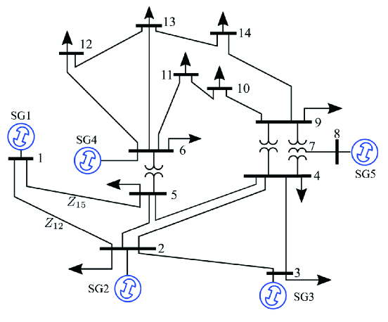
Figure 1: IEEE 14-bus power system

Each bus is modeled as a subsystem using a descriptor system. For the $k$-th synchronous machine on the bus, the differential equations governing its model are:

$$\frac{di_{d}^{[k]}}{dt} =\frac{v_{d}^{[k]}-R^{[k]}i_{d}^{[k]}+w^{[k]}(L^{[k]}i_{q}^{[k]}-\psi_{f}^{[k]})}{L^{[k]}},$$

$$\frac{di_{q}^{[k]}}{dt} =\frac{v_{q}^{[k]}-R^{[k]}i_{q}^{[k]}-w^{[k]}(L^{[k]}i_{d}^{[k]})}{L^{[k]}},$$

$$\frac{dw^{[k]}}{dt} =\frac{\psi_{f}^{[k]}i_{d}^{[k]}-T_{m}^{[k]}-D^{[k]}w^{[k]}}{J^{[k]}},$$

$$\frac{d\theta^{[k]}}{dt} =w^{[k]}.$$

These equations depict the dynamics of the synchronous machine in the $dq$-reference frame, where $i_{d}^{[k]}$ and $i_{q}^{[k]}$ are the direct and quadrature axis currents, $v_{d}^{[k]}$ and $v_{q}^{[k]}$ are the corresponding voltages. Here, $\psi_{f}^{[k]}$ represents the field flux linkage, and $T_{m}^{[k]}$ is the mechanical torque input. The parameters $R^{[k]}$, $L^{[k]}$, $D^{[k]}$, $J^{[k]}$, and $w^{[k]}$ denote the resistance, inductance, damping coefficient, inertia, and rotor speed, respectively.

The connections between buses, represented by parameters such as resistances and reactances, are considered as the parameters of the subsystem connections to be identified. The internal inputs of the NDS are the bus voltages $v_{d}^{[k]}$ and $v_{q}^{[k]}$, while the internal outputs are the bus currents $i_{d}^{[k]}$ and $i_{q}^{[k]}$. The external input is the mechanical torque $T_{m}^{[k]}$. To ensure Assumption 6, which requires the matrix $G_{yv}(\lambda)$ to have full column rank, the external outputs are chosen as $i_{d}^{[k]}$, $i_{q}^{[k]}$, $w^{[k]}$, and $\theta^{[k]}$. This selection guarantees that the necessary conditions for system identifiability and moment estimation are satisfied.

A load flow analysis was performed to determine the operating point of the NDS. The nonlinear synchronous machine model was then linearized around this equilibrium point to obtain a descriptor system representation suitable for identification. The goal of the identification process was to estimate the interconnection parameters (e.g., resistances and reactances) between buses using the measured bus currents. To simplify computations and avoid emergent phenomena in networked systems, only four parameters (two resistances and two reactances) were randomly selected for identification.

It has been verified that for this NDS, only one frequency point is required for the signal-generation system $\Sigma_{s}$ to achieve identification. The frequency $1\,\,\mathrm{rad}/\mathrm{s}$ was selected, with the matrix $\Pi$ being a randomly generated invertible matrix and $\xi(0)$ being a randomly generated nonzero vector. The corresponding Nyquist sampling frequency for this NDS is $7.11\,\,\mathrm{Hz}$, with the minimum sampling time being $0.1407\,\,\mathrm{s}$. The sampling intervals for the five generators were randomly selected within the range of 0.1 s to 0.5 s (which can be higher than the minimum sampling interval corresponding to the Nyquist frequency). The upper bound of the steady-state settling time is $\bar{t}_{s}=14.25\,\mathrm{s}$.

Due to space limitations, only the convergence behavior of the two-stage algorithm is presented.

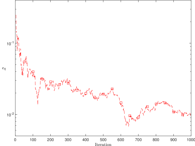
Figure 2: Norm of Relative Estimation Error of $\bar{\eta}$

Figure 2 shows the relative error of the zero-order moment estimation of NDS, calculated as $e_{\bar{\eta}}=\left\|\frac{\bar{\eta}-\eta}{\eta}\right\|_{2}$.

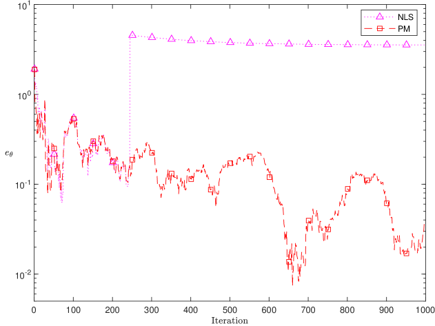
Figure 3: Norm of Relative Estimation Error of $\theta$

Figure 3 presents the relative error of parameter estimation, which is compared with the nonlinear least-squares method. The relative error is computed as $e_{\theta}=\left\|\frac{\bar{\theta}-\theta}{\theta}\right\|_{2}$.

The simulation results confirm the efficacy of the proposed two-stage algorithm in accurately recovering the interconnection parameters of the NDS. By leveraging the steady-state response and recursively updating the zeroth-order moment estimates, the algorithm achieves robust performance even under highly irregular sampling conditions. Furthermore, the comparison with the nonlinear least-squares algorithm highlights that the proposed algorithm effectively avoids the issue of the optimization process getting trapped in local minima, a common challenge with NLS, while ensuring global convergence.

V Conclusions

This paper addresses the challenge of structure identification for NDS with descriptor subsystems under non-synchronous, non-uniform, and slow-rate sampling conditions. By bridging system identification with model reduction techniques, we propose a novel two-stage algorithm that leverages zero-order moments to reconstruct subsystem interconnections explicitly. Key contributions and findings are summarized as follows:

• Unified Handling of Sampling Irregularities: The proposed method generalizes existing approaches by simultaneously accommodating asynchronous, non-uniform, and low-rate sampling. This eliminates constraints on input signal periodicity and extends applicability to multi-input multi-output NDS with arbitrary interconnections.

• Zero-Order Moment-Based Framework: By estimating zero-order moments from steady-state outputs and linking them to subsystem interconnections, our approach avoids black-box modeling limitations. This enables explicit recovery of structural parameters while preserving the physical interpretability of the NDS.

• Robust Numerical Validation: Simulations on the IEEE 14-bus power system demonstrate rapid convergence and high accuracy in parameter estimation, even under significant sampling irregularities. The algorithm outperforms nonlinear least-squares methods by avoiding local minima traps, highlighting its reliability for real-world applications.

Future work will focus on extending this approach to systems with repeated eigenvalues or higher-order moments, as well as its application to more complex networked systems with nonlinear dynamics.

Proof of Corollary 1:

Consider the state-space representation of the system dynamics:

$$\xi(t)=Te^{\Lambda t}T^{-1}\xi(0)$$

The inverse transformation matrix $T^{-1}$ is block-diagonal with two components:

$$T^{-1}=\text{diag}\left\{I_{m_{r}},\underbrace{\frac{1}{2}\begin{bmatrix}1&-j\\ 1&j\end{bmatrix},\dots,\frac{1}{2}\begin{bmatrix}1&-j\\ 1&j\end{bmatrix}}_{m_{c}\text{ blocks}}\right\}$$

Applying $T^{-1}$ to $\xi(0)$ yields:

$$T^{-1}\xi(0)=\text{col}\left\{\alpha_{i}\big{|}_{i=1}^{m_{r}},\frac{1}{2}\begin{bmatrix}\beta_{i}^{*}\\ \beta_{i}\end{bmatrix}\bigg{|}_{i=1}^{m_{c}}\right\}$$

The matrix exponential $e^{\Lambda t}$ is block-diagonal:

$$e^{\Lambda t}=\text{diag}\left\{e^{\lambda_{r,i}t}\big{|}_{i=1}^{m_{r}},\begin{bmatrix}e^{\lambda_{c,i}t}&0\\ 0&e^{\lambda_{c,i}^{*}t}\end{bmatrix}\bigg{|}_{i=1}^{m_{c}}\right\}$$

The output $y_{s}(t)$ is obtained through:

$$y_{s}(t)=\begin{bmatrix}\mathscr{R}&\mathscr{C}\end{bmatrix}e^{\Lambda t}T^{-1}\xi(0)$$

Expanding this product yields two components. For each real eigenvalue $\lambda_{r,i}$:

$$\alpha_{i}e^{\lambda_{r,i}t}\eta_{0}(\lambda_{r,i};\pi_{r,i})$$

For each complex pair $\lambda_{c,i},\lambda_{c,i}^{*}$:

$$\frac{1}{2}\beta_{i}^{*}e^{\lambda_{c,i}t}\eta_{0}(\lambda_{c,i};\pi_{c,i})+\frac{1}{2}\beta_{i}e^{\lambda_{c,i}^{*}t}\eta_{0}(\lambda_{c,i}^{*};\pi_{c,i}^{*})$$

Using the identity for complex conjugates: $\text{Re}\{z\}=\frac{1}{2}(z+z^{*})$ and the conjugate symmetry of $\eta_{0}(\lambda_{c,i};\pi_{c,i})$.

Summing all contributions gives the total response:

$$y_{s}(t)= \sum_{i=1}^{m_{r}}\alpha_{i}e^{\lambda_{r,i}t}\eta_{0}\left(\lambda_{r,i};\pi_{r,i}\right)$$

$$+\sum_{i=1}^{m_{c}}\operatorname{Re}\left\{\beta_{i}^{*}e^{\lambda_{c,i}t}\eta_{0}\left(\lambda_{c,i};\pi_{c,i}\right)\right\}$$

This completes the proof.  ∎

Proof of Theorem 2:

For $\star=r$, where $i=1,2,\dots,m_{r}$, and $\star=c$, where $i=1,2,\dots,m_{c}$, when Assumption 6 is satisfied, the following relationship holds:

$$G_{yv}^{\dagger}(\lambda_{\star,i})G_{yu}\left(\lambda_{\star,i}\right)=I_{m_{u}}$$

From (6), it follows that:

$$\left[I_{m_{v}}-\Phi(\theta)G_{zv}(\lambda_{\star,i})\right]^{-1}\Phi(\theta)G_{zu}(\lambda_{\star,i})\pi_{\star,i}$$

$$= \kappa_{\star,i}+G_{yv}^{\dagger}(\lambda_{\star,i})e_{\star,i}$$

Under Assumption 1, the matrix $I_{m_{v}}-\Phi(\theta)G_{zv}(\lambda_{\star,i})$ is invertible for $\lambda_{\star,i}$. Combining the terms involving $\theta$ yields:

$$\Phi(\theta)\left\{G_{zu}(\lambda_{\star,i})\pi_{\star,i}+G_{zv}(\lambda_{\star,i})\kappa_{\star,i}\right\}=\kappa_{\star,i}+\tilde{e}_{\star,i}$$

Since the matrix $\Phi(\theta)$ has the following structural constraint:

$$\Phi(\theta)=\sum_{i=1}^{m_{\theta}}{\theta_{i}\Phi_{i}}$$

where $\Phi_{i}$ are known real-valued matrices and $\theta_{i}\in\mathbb{R}$ for $i=1,2,\cdots,m_{\theta}$, the following relationships are derived. For real eigenvalues $\lambda_{r,i}$ with $i=1,2,\cdots,m_{r}$:

$$\sum_{j=1}^{m_{\theta}}{\theta_{j}\Phi_{j}\psi_{r,i}}=\kappa_{r,i}+\tilde{e}_{r,i}$$

Vectorizing this equation results in:

$$\psi_{r,i}^{T}\otimes I_{m_{v}}\cdot\varPsi_{p}\theta=\kappa_{r,i}+\tilde{e}_{r,i}$$

Similarly, for complex eigenvalues $\lambda_{c,i}$ with $i=1,2,\cdots,m_{c}$, separating the real and imaginary parts gives:

$$\mathrm{Re}\{\psi_{c,i}^{T}\}\otimes I_{m_{v}}\cdot\varPsi_{p}\theta =\mathrm{Re}\{\kappa_{c,i}+\tilde{e}_{c,i}\}$$

$$\mathrm{Im}\{\psi_{c,i}^{T}\}\otimes I_{m_{v}}\cdot\varPsi_{p}\theta =\mathrm{Im}\{\kappa_{c,i}+\tilde{e}_{c,i}\}$$

Based on the definitions of $\kappa$ and $\tilde{e}$ in (15), the following explicit representation of the parameter $\theta$ is obtained:

$$\varUpsilon^{T}\otimes I_{m_{v}}\cdot\varPsi_{p}\theta=\kappa+\tilde{e}$$

The proof is completed according to (16).  ∎

References

- [1] V. Chetty, S. Warnick, S. Roy, and S. Das, “Meanings and applications of structure in networks of dynamic systems,” in Principles of Cyber-Physical Systems: An Interdisciplinary Approach. Cambridge Univ. Press, 2020, pp. 162–201.
- [2] Y. Wang, A. Li, and L. Wang, “Networked dynamic systems with higher-order interactions: stability versus complexity,” National Science Review, Mar. 2024.
- [3] T. Zhou, K. You, and L. Tao, Estimation and Control of Large-scale Networked Systems. Butterworth-Heinemann, 2018.
- [4] L. Ljung, System Identification:Theory for the User(2nd ed.). Upper Saddle River, NJ, USA: Prentice-Hall, 1999.
- [5] T. Zhou, “Identification of lft structured descriptor systems with slow and non-uniform sampling,” arXiv preprint arXiv:2407.00629, 2024.
- [6] M. F. Shakib, G. Scarciotti, A. Y. Pogromsky, A. Pavlov, and N. van de Wouw, “Time-domain moment matching for multiple-input multiple-output linear time-invariant models,” Automatica, vol. 152, p. 110935, 2023.
- [7] I. Necoara and T. C. Ionescu, “ model reduction of linear network systems by moment matching and optimization,” IEEE Transactions on Automatic Control, vol. 65, no. 12, pp. 5328–5335, 2020.
- [8] A. Astolfi, “Model reduction by moment matching for linear and nonlinear systems,” IEEE Transactions on Automatic Control, vol. 55, no. 10, pp. 2321–2336, 2010.
- [9] E. de Souza and S. Bhattacharyya, “Controllability, observability and the solution of ax-xb= c,” Linear Algebra and its Applications, vol. 39, pp. 167–188, 1981.
- [10] J. Ball, I. Gohberg, et al., Interpolation of rational matrix functions. Birkhäuser, 2013, vol. 45.
- [11] P. Benner, P. Goyal, and P. Van Dooren, “Identification of port-hamiltonian systems from frequency response data,” Systems & Control Letters, vol. 143, p. 104741, 2020.
- [12] A. Moreschini, J. D. Simard, and A. Astolfi, “Data-driven model reduction for port-hamiltonian and network systems in the loewner framework,” Automatica, vol. 169, p. 111836, 2024.
- [13] P. Van Dooren, K. A. Gallivan, and P.-A. Absil, “H2-optimal model reduction of mimo systems,” Applied Mathematics Letters, vol. 21, no. 12, pp. 1267–1273, 2008.
- [14] R. V. Polyuga and A. Van der Schaft, “Structure preserving model reduction of port-hamiltonian systems by moment matching at infinity,” Automatica, vol. 46, no. 4, pp. 665–672, 2010.
- [15] N. Bousselmi, J. M. Hendrickx, and F. Glineur, “Interpolation conditions for linear operators and applications to performance estimation problems,” SIAM Journal on Optimization, vol. 34, no. 3, pp. 3033–3063, 2024.
- [16] S. Gugercin, R. V. Polyuga, C. Beattie, and A. Van Der Schaft, “Structure-preserving tangential interpolation for model reduction of port-hamiltonian systems,” Automatica, vol. 48, no. 9, pp. 1963–1974, 2012.
- [17] I. V. Gosea and A. C. Antoulas, “The one-sided loewner framework and connections to other model reduction methods based on interpolation,” IFAC-PapersOnLine, vol. 55, no. 30, pp. 377–382, 2022.