Magnetic Field Dynamics and Energy Dissipation of Relativistic Magnetohydrodynamics in Relativistic Heavy-Ion Collisions

Abstract

Abstract: We systematically explore the interplay between time-dependent magnetic fields and energy density evolution in relativistic magnetohydrodynamics (RMHD), focusing on ultra-relativistic and magnetized conformal fluids. Three characteristic magnetic field evolution models (Type-1, Type-2, Type-3), parameterized to reflect temporal profiles observed in relativistic heavy-ion collisions, are integrated into a (1 + 1) D Bjorken-flow framework. For both fluid types, stronger magnetic fields universally suppress energy dissipation, with suppression magnitudes ordered as Type-1 $>$ Type-2 $>$ Type-3, driven by distinct decay rates of magnetic energy. To bridge QCD physics with macroscopic dynamics, we further incorporate a temperature-dependent magnetic susceptibility ($\chi_{m}(T)$) derived from lattice QCD, capturing the transition from diamagnetic hadronic matter ($\chi_{m}<0$) to paramagnetic quark-gluon plasma ($\chi_{m}>0$). Our simulations reveal that $\chi_{m}(T)$ introduces a feedback loop: delayed energy dissipation sustains higher temperatures, reinforcing paramagnetic behavior and altering field evolution. These results quantify the critical role of magnetic field dynamics in regulating QGP thermalization and highlight the necessity of QCD-informed susceptibilities for realistic RMHD modeling.

I Introduction

Relativistic heavy-ion collision experiments at facilities like the Relativistic Heavy Ion Collider (RHIC) provide a unique laboratory to study the properties of quantum chromodynamic (QCD) matter under extreme conditions. In such collisions, the interaction of two highly Lorentz-contracted nuclei generates a hot, dense medium dominated by deconfined quarks and gluons-the quark-gluon plasma (QGP)Adams et al. (2005); Gyulassy and McLerran (2005). This short-lived state exhibits near-perfect fluidity, enabling relativistic hydrodynamic models to successfully describe its collective expansion and thermalization dynamicsHeinz and Kolb (2002); Hirano et al. (2006); Guo et al. (1999); Moreland et al. (2015); Shuryak (2004); Heinz and Snellings (2013). Notably, the interplay between hydrodynamic evolution and electromagnetic phenomena has emerged as a critical frontier in understanding QGP behavior, particularly in non-central collisions where ultra-strong magnetic fields ( $10^{18}\sim 10^{19}$ Gauss) are transiently generatedBzdak and Skokov (2012); Deng and Huang (2012); Tuchin (2013); Mo et al. (2013); Zhong et al. (2014, 2015); Roy and Pu (2015); Li et al. (2016).

These magnetic fields, though short-lived in vacuumKharzeev et al. (2008), persist longer in the electrically conductive QGP mediumShe et al. (2018); Chen and Feng (2020); Chen et al. (2021); Kharzeev and Warringa (2009), creating opportunities to probe magnetohydrodynamic effects. Key phenomena such as the Chiral Magnetic Effect (CME)Fukushima et al. (2008); Guo et al. (2019), Chiral Separation Effect (CSE)Aghababaie and Burgess (2004), and their collective manifestation as Chiral Magnetic Waves (CMWs)Kharzeev and Yee (2011); Burnier et al. (2011) are theorized to induce charge-dependent azimuthal anisotropies in particle emissionJiang et al. (2024). However, disentangling these signals from background collective flow remains experimentally challengingKhachatryan et al. (2017); Sirunyan et al. (2018, 2019), necessitating precise theoretical modeling of the coupled evolution of the QGP and electromagnetic fieldsQiu and Feng (2023); Zhu and Feng (2023); Deng and Feng (2022); Qiu et al. (2023); Bao and Feng (2024); Feng et al. (2020); Zhu et al. (2019); Feng et al. (2018). Relativistic magnetohydrodynamics (RMHD) offers a self-consistent framework to explore this coupling. While prior studies have examined simplified scenarios, the time-dependent evolution of magnetic fields particularly their dependence on proper time ($\tau$) in the RHIC energy regime remains under explored in (1 + 1) D RMHD frameworks. This gap limits our ability to quantify how magnetic field dissipation shapes energy density dynamics and thermalization processes in the QGP.

In this work, we address this challenge by integrating three distinct models of time-dependent magnetic field evolution into a (1 + 1) D relativistic magnetohydrodynamic framework based on Bjorken flowBjorken (1983). These models (Type-1, Type-2 and Type-3) capture characteristic $\tau$-dependences observed in RHIC-energy collisions Müller and Schäfer (2018); Jiang et al. (2018); Shi et al. (2018). We systematically analyze their impact on energy dissipation in two fluid scenarios: (1) an ultra-relativistic fluid with a simplified equation of state ( $p=c_{s}^{2}e$ ), and (2) a magnetized conformal fluid incorporating explicit magnetization effects. To enhance physical realism, we further introduce a temperature-dependent magnetic susceptibility ( $\chi_{m}(T)$ ) derived from lattice QCD calculationsBali et al. (2014a); Bonati et al. (2013, 2014a); Levkova and DeTar (2014); Bonati et al. (2014b); Simonov and Orlovsky (2015); Bali et al. (2014b), which encodes the transition from diamagnetic hadronic matter ( $\chi_{m}<0$ ) to paramagnetic QGP ( $\chi_{m}>0$).

Our study aims to resolve two pivotal questions: (1) How do the temporal profiles of magnetic fields in the RHIC regime influence the energy density evolution of QGP? (2) What role does the phase structure of Quantum Chromodynamics (QCD), manifested through temperature (T), play in regulating electromagnetic response and energy dissipation? By bridging first-principles QCD inputs with macroscopic RMHD simulations, this work advances the quantitative understanding of magnetized QGP dynamics. The results not only clarify the interplay between magnetic field decay and hydrodynamic expansion but also establish benchmarks for future studies incorporating dissipative effects and spatial inhomogeneities.

The paper is organized as follows: Section II outlines the RMHD formalism with magnetization. Section III adapts Bjorken flow to incorporate external magnetic fields. Section IV compares energy density evolution across the three magnetic field models for both fluid types. Section V integrates lattice QCD-derived $\chi_{m}(T)$ and a realistic equation of state. Section VI summarizes key findings and discusses implications for heavy-ion physics.

II Formulas of Magnetohydrodynamics

In this section, we provide a brief introduction to the Lorentz-covariant formulation of ideal magnetohydrodynamics (MHD) with nonzero magnetization. The total energy-momentum tensor of relativistic ideal magnetohydrodynamics can be decomposed into two parts

$$T^{\mu\nu}=T^{\mu\nu}_{M}+T^{\mu\nu}_{EM},$$ (1)

where the energy-momentum tensor of the electromagnetic field is given by

$$T^{\mu\nu}_{\text{EM}}=-F^{\mu\lambda}F^{\nu}_{\ \lambda}+\frac{1}{4}g^{\mu\nu}F^{\alpha\beta}F_{\alpha\beta},$$ (2)

and the energy-momentum tensor of the fluid is given by

$$T^{\mu\nu}_{M}=eu^{\mu}u^{\nu}-p\Delta^{\mu\nu}-\frac{1}{2}(M^{\nu\lambda}F^{\mu}_{\lambda}+M^{\mu\lambda}F^{\nu}_{\lambda}),$$ (3)

where $F^{\mu\nu}$ is the field strength tensor, and $M^{\mu\nu}$ is the polarization tensor. In the weak-field limit, the $M^{\mu\nu}$ associated terms can be neglected.

$$\partial_{\mu}T^{\mu\nu}=0.$$ (4)

Using Maxwell’s equations, the aforementioned equation can be rewritten as

$$\partial_{\mu}T^{\mu\nu}_{M}=-\partial_{\mu}T^{\mu\nu}_{EM}=F^{\nu\lambda}j_{\lambda},$$ (5)

where $j^{\mu}$ is the four-current density, and the electromagnetic field strength tensor can be decomposed as

$$F^{\mu\nu}=E^{\mu}u^{\nu}-E^{\nu}u^{\mu}+\varepsilon^{\mu\nu\alpha\beta}u_{\alpha}B_{\beta}\ .$$ (6)

We consider a non-viscous fluid coupled with a magnetic field, assuming that the medium is fully conductive and the four-vector electric field is zero in the comoving reference frame. By substituting the electromagnetic field tensor into the energy-momentum tensor of ideal magnetohydrodynamics with magnetization, we obtain

$$T^{\mu\nu}=\left(e+p-MB+B^{2}\right)u^{\mu}u^{\nu}-\left(p-MB+\frac{B^{2}}{2}\right)g^{\mu\nu}+\left(MB-B^{2}\right)b^{\mu}b^{\nu},$$ (7)

where $e$, $P$, $B$, $M=\chi_{m}B$, and $\chi_{m}$ denote the energy density, the pressure, the magnetic field strength, the magnetization intensity and the magnetic susceptibility in the local rest frame of the fluid, respectively.

The projection of energy-momentum along the four-dimensional velocity vector $u^{\nu}$ corresponds to the conservation of fluid energy, and its form is as follows:

$$\begin{split}0&=u_{\nu}\partial_{\mu}T^{\mu\nu}\\ &=u^{\alpha}\partial_{\alpha}e+Bu^{\alpha}u_{\alpha}B+(e+p)\partial_{\alpha}u^{\alpha}-MB\partial_{\alpha}u^{\alpha}\\ &\quad+B^{2}\partial_{\alpha}u^{\alpha}+MBu_{\mu}b^{\nu}\partial_{\nu}b^{\mu}-B^{2}u_{\mu}b^{\nu}\partial_{\nu}b^{\mu}\\ &=u^{\alpha}\partial_{\alpha}e+(e+p)\partial_{\alpha}u^{\alpha}+Mu^{\alpha}\partial_{\alpha}B,\end{split}$$ (8)

where $u_{\nu}u^{\nu}=1$, $u_{\nu}b^{\nu}=0$, and $u_{\nu}\partial_{\mu}u^{\nu}=0$ are taken. The Maxwell equationPu et al. (2016) is given by

$$\frac{1}{2}(u^{\alpha}\partial_{\alpha})B^{2}+B^{2}\partial_{\alpha}u^{\alpha}+B^{2}b^{\mu}b^{\nu}\partial_{\nu}u_{\mu}=0\ ,$$ (9)

Similarly, the projection of the energy-momentum along the direction orthogonal to the four-velocity $u^{\mu}$ corresponds to the momentum conservation, and its expression is

$$\begin{split}0&=\Delta_{\nu\alpha}\partial_{\mu}T^{\mu\nu}\\ &=\Delta_{\nu\alpha}(e+p-MB+B^{2})u^{\mu}\partial_{\mu}u^{\nu}+\Delta_{\nu\alpha}(e+p-MB+B^{2})u^{\nu}\partial_{\mu}u^{\mu}\\ &\quad-\Delta_{\nu\alpha}\partial^{\nu}(p-MB+\frac{B^{2}}{2})+\Delta_{\nu\alpha}(MB-B^{2})\partial_{\mu}(b^{\mu}b^{\nu})+\Delta_{\nu\alpha}b^{\mu}b^{\nu}\partial_{\mu}(MB-B^{2})\,,\\ &=(e+p-MB+B^{2})u^{\mu}\partial_{\mu}u_{\alpha}-\Delta_{\nu\alpha}\partial^{\nu}(p-MB+\frac{B^{2}}{2})\\ &\quad+\Delta_{\nu\alpha}\partial_{\mu}[(MB-B^{2})b^{\mu}b^{\nu}],\end{split}$$ (10)

and the last term of Eq. (10) is given as

$$\Delta_{\nu\alpha}\partial_{\mu}[(MB-B^{2})b^{\mu}b^{\nu}]=(\chi_{m}-1)\left[\partial_{\mu}(B^{\mu}B^{\alpha})-u_{\nu}u^{\alpha}\partial_{\mu}(B^{\mu}B^{\nu})\right]\ ,$$ (11)

where the magnetization coefficient $\chi_{m}$ is constantLi and Yee (2018). It is found that the last term of Eq. (11) vanishes. The simplified momentum conservation becomes

$$0 =\Delta_{\nu\alpha}\partial_{\mu}T^{\mu\nu}$$

$$=(e+p-MB+B^{2})u^{\mu}\partial_{\mu}u_{\alpha}-\Delta_{\nu\alpha}\partial^{\nu}\left(p-MB+\frac{B^{2}}{2}\right).$$ (12)

where one uses $\Delta_{\nu\alpha}u^{\nu}=0$.

III Bjorken flow

In the work, we consider a fluid undergoing Bjorken expansion. For longitudinally boost-invariant flow, Milne coordinates are more convenient than standard Cartesian coordinates $(t,x,y,z)$. Milne coordinates are $x^{\mu}=(\tau,x,y,\eta_{s})$, which are natural choices for describing ultra-relativistic heavy-ion collisionJaiswal et al. (2019), where $\tau=\sqrt{t^{2}-z^{2}}$ is the proper time and $\eta_{s}=\tanh^{-1}(z/t)$ is the pseudorapidity.

The Bjorken flowBjorken (1983) is uniform in the transverse direction and exhibits longitudinal boost-invariance. Its symmetry lies in the transverse plane $(x-y$ plane), enhancing invariance along the longitudinal (or beam) direction, and also exhibiting reflection symmetry $(z\rightarrow-z)$. This implies that the flow profile $v^{x}=v^{y}=0$ and $v^{z}=z/t$ are symmetric in the transverse plane and invariant along the longitudinal directionJaiswal et al. (2022). The fluid velocity can be taken as

$$u^{\mu}=\left(\frac{t}{\tau},0,0,\frac{z}{t}\right),$$ (13)

and all macroscopic quantities depend only on proper time $\tau$, independent of spatial coordinates and four-velocity.

Using Milne coordinates, one can simplify the four-velocity to $u^{\mu}=(1,\vec{0})$. The spatial derivatives and the four-divergence can be taken as

$$u^{\mu}\partial_{\mu}=\partial_{\tau},\partial_{\alpha}u^{\alpha}=\theta=\frac{1}{\tau}.$$ (14)

In addition to the direction of fluid velocity, the magnetic field also chooses another special direction related to the spatial unit vector $b^{\mu}=B^{\mu}/B$, where $B=\sqrt{-B^{\mu}B_{\mu}}$ is normalized to $b^{\mu}b_{\mu}=-1$. In this work, it is assumed that the magnetic field is perpendicular to the reaction plane and oriented along the $y$-axis. The fluid in which the magnetic field is located has infinite conductivity and nonzero magnetization $B^{\mu}=(0,0,B_{y},0)$Karimabadi et al. (2023). In this case, the magnetic field remains unchanged in Milne coordinates, and the magnetic flux freezing theorem gives

$$\partial_{\tau}\left(\frac{B}{s}\right)=0,$$ (15)

where $s$ is the entropy density, that is, $B/s$ is a conserved quantity, which means:

$$\frac{B}{B_{0}}=\frac{s}{s_{0}},$$ (16)

where $B_{0}$ and $s_{0}$ are the initial magnetic field and the entropy density, respectively.

For fluids in thermodynamic equilibrium, certain properties can be determined (see, for example, Refs. Caldarelli et al. (2009); Huang et al. (2010); Kamikado and Kanazawa (2015)) as

$$e+p=Ts+\mu n,$$ (17)

where $n$ and $\mu$ are the baryon number density and the corresponding chemical potential, respectively. According to thermodynamic relationship, one can obtain

$$de=Tds+\mu dn-MdB,$$ (18)

and

$$dp=sdT+nd\mu+MdB\,.$$ (19)

In ultra-relativistic heavy ion collisions, the net baryon number density and chemical potential are nearly zero at mid-rapidity region. Therefore, we study the case where the chemical potential of the baryons is zero in this study.

IV Fluid Evolution Under Three Different Magnetic Field Conditions

Within the linear approximation, the effects of magnetization can be characterized by the magnetic susceptibility. Numerous studies, including those based on lattice QCD Bali et al. (2014a); Bonati et al. (2013, 2014a); Levkova and DeTar (2014); Bonati et al. (2014b); Simonov and Orlovsky (2015); Bali et al. (2014b), perturbative QCD Bergman et al. (2008), the Sakai-Sugimoto model Cherman et al. (2009), the functional renormalization group approach Bergman et al. (2008), and other theoretical frameworksSimonov and Orlovsky (2015); Steinert and Cassing (2014); Kabat et al. (2002); Anber and Ünsal (2014); Tawfik and Magdy (2014); Bali et al. (2020), have suggested that the medium exhibits diamagnetic behavior in the confined phase, i.e., $\chi_{m}<0$, while displaying paramagnetic behavior in the deconfined QGP phase, i.e., $\chi_{m}>0$. In this work, we focus solely on the behavior of the magnetic field in the deconfined phase. For simplicity, we assume that the magnetic susceptibility $\chi_{m}$ remains constant throughout this section. The energy conservation equation becomes

$$\partial_{\tau}e+\frac{(e+p-MB+B^{2})}{\tau}+\frac{1}{2}\partial_{\tau}B^{2}=0\,,$$ (20)

since the magnetic field is non-zero only in the $y$ direction, there exists $-B^{2}u_{\mu}b^{\nu}\partial_{\nu}b^{\mu}=0=MBu_{\mu}b^{\nu}\partial_{\nu}b^{\mu}$. Inserting into Eq.(20), one can obtain

$$\partial_{\tau}e+\frac{e+p}{\tau}+\frac{1}{2}\partial_{\tau}B^{2}=0\ .$$ (21)

Assuming that in relativistic heavy ion collisions, the magnetic field $B_{y}(\tau,\vec{x})=B_{0}(\vec{x})F_{B}(\tau_{B},\tau)$  Guo et al. (2019) is along the $y$ direction, where $B_{0}$ represents the magnitude of the initial magnetic field. Considering three different parameterization methods commonly used in the literature Müller and Schäfer (2018); Jiang et al. (2018); Shi et al. (2018) for the variation of magnetic fields with proper time, these methods are employed to study various magnetic field effects in relativistic heavy ion collisions, specifically:

Type-1:

$$F_{B}(\tau_{B},\tau)=\frac{1}{1+(\tau-\tau_{0})^{2}/\tau_{B}^{2}}\,,$$ (22)

Type-2:

$$F_{B}(\tau_{B},\tau)=\frac{1}{[1+(\tau-\tau_{0})^{2}/\tau_{B}^{2}]^{3/2}}\,,$$ (23)

and Type-3:

$$F_{B}(\tau_{B},\tau)=e^{-|\tau-\tau_{0}|/\tau_{B}}\,.$$ (24)

In all these parameterizations, $\tau_{B}$ is the fundamental magnetic field lifetime parameter that controls the rate at which the magnetic field decreases over time. However, it should be noted that due to differences in their functional forms, the evolution of the magnetic field varies slightly for the same $\tau_{B}$ valueGuo et al. (2019). In this study, it is assumed that $\tau_{B}$ is comparable to $\tau_{0}$, meaning that the lifetime of the magnetic field is similar to the initial time of hydrodynamic evolution. This assumption implies that the magnetic field exists during the early stages of hydrodynamic evolution but gradually vanishes over time. The required lifetime $\tau_{B}$ decreases with increasing beam energy. For example, $\tau_{B}\sim 5~\text{fm/c}$ for $\sqrt{s_{NN}}=11.5$ GeV, $\tau_{B}\sim 0.5~\text{fm/c}$ for $\sqrt{s_{NN}}=200$ GeV. Parameter $A=92$ for type-1, $A=125$ for type-2 and $A=128$ for type-3. An average over these three types of time dependence in a (perhaps naive) statistical way would suggest $\tau_{B}=A/\sqrt{s_{NN}}$ with $A=115\pm 16~\text{GeV}\times~\text{fm}/c$. In this paper, we consider collisions with $\sqrt{s_{NN}}$ = 200 GeV in the RHIC energy region.

IV.1 Ultra-relativistic Fluid

Since the fluid is considered as ultra-relativistic, the contribution of the rest mass to the equation of state (EOS) can be neglected. The pressure is proportional to the energy density, i.e., $p=c_{s}^{2}e$, where $c_{s}$ is the local sound speed, which is assumed to be constant ($c_{s}=1/\sqrt{3}$).

Some dimensionless quantities $\tilde{e}=e/e_{0}$ and $\sigma_{0}=B_{0}^{2}/e_{0}$ are defined to describe the normalized energy density, and initial magnetic field parameter, respectively, where $e_{0}$ represents the initial energy density.

Substituting the magnetic field decay models under the three different modes into Eq. (21), we obtain the following form:

Type-1:

$$\partial_{\tau}\tilde{e}+\left(1+c_{s}^{2}\right)\frac{\tilde{e}}{\tau}-\frac{2\chi_{m}(\tau-\tau_{0})\sigma_{0}}{\left[1+\left(\frac{\tau-\tau_{0}}{\tau_{B}}\right)^{2}\right]^{3}\tau_{B}^{2}}=0,$$ (25)

Type-2:

$$\partial_{\tau}\tilde{e}+\left(1+c_{s}^{2}\right)\frac{\tilde{e}}{\tau}-\frac{3\chi_{m}(\tau-\tau_{0})\tau_{B}^{6}\sigma_{0}}{\left(\tau^{2}-2\tau\tau_{0}+\tau_{0}^{2}+\tau_{B}^{2}\right)^{4}}=0,$$ (26)

Type-3:

$$\partial_{\tau}\tilde{e}+\left(1+c_{s}^{2}\right)\frac{\tilde{e}}{\tau}-\frac{\chi_{m}\sigma_{0}e^{-\frac{2|\tau-\tau_{0}|}{\tau_{B}}}}{\tau_{B}}\frac{\partial|\tau-\tau_{0}|}{\partial\tau}=0.$$ (27)

Figure 1 investigates the evolution of energy density in an ultra-relativistic fluid under the influence of time-dependent magnetic fields in the relativistic heavy-ion collisions within the framework of relativistic magnetohydrodynamics (RMHD). The figure depicts three different magnetic field evolution models (Type-1, Type-2, and Type-3) while considering various magnetic field values of $\sigma_{0}$. The black solid line represents the case without a magnetic field, whereas the red dotted line, blue dashed line, orange dash-dotted line, and green dash-dotted line correspond to $\sigma_{0}$ = 0.5, 5, 10 and 25, respectively. Specifically, it examines how three distinct magnetic field evolution models (Type-1, Type-2, and Type-3 in relativistic heavy-ion collisions) affect the decay rate of energy density as a function of proper time ($\tau$). The study highlights the interplay between magnetic field strength (parameterized time ($\tau$))by $\sigma_{0}$) and energy dissipation dynamics. All models demonstrate that stronger magnetic fields ($\sigma_{0}$) decelerate energy dissipation compared to the non-magnetized case (black solid line). Magnitude of suppression is shown by Type-1 $>$ Type-2 $>$ Type-3 exhibits unique behavior with faster early-stage decay for weak fields, diverging from the monotonic trends of Type-1 and Type-3.

Figure 1 underscores the critical role of magnetic field evolution models in shaping energy density dynamics. The study bridges theoretical RMHD frameworks with relativistic heavy-ion experimental, emphasizing the need for precise modeling of magnetic fields in high-energy physics.

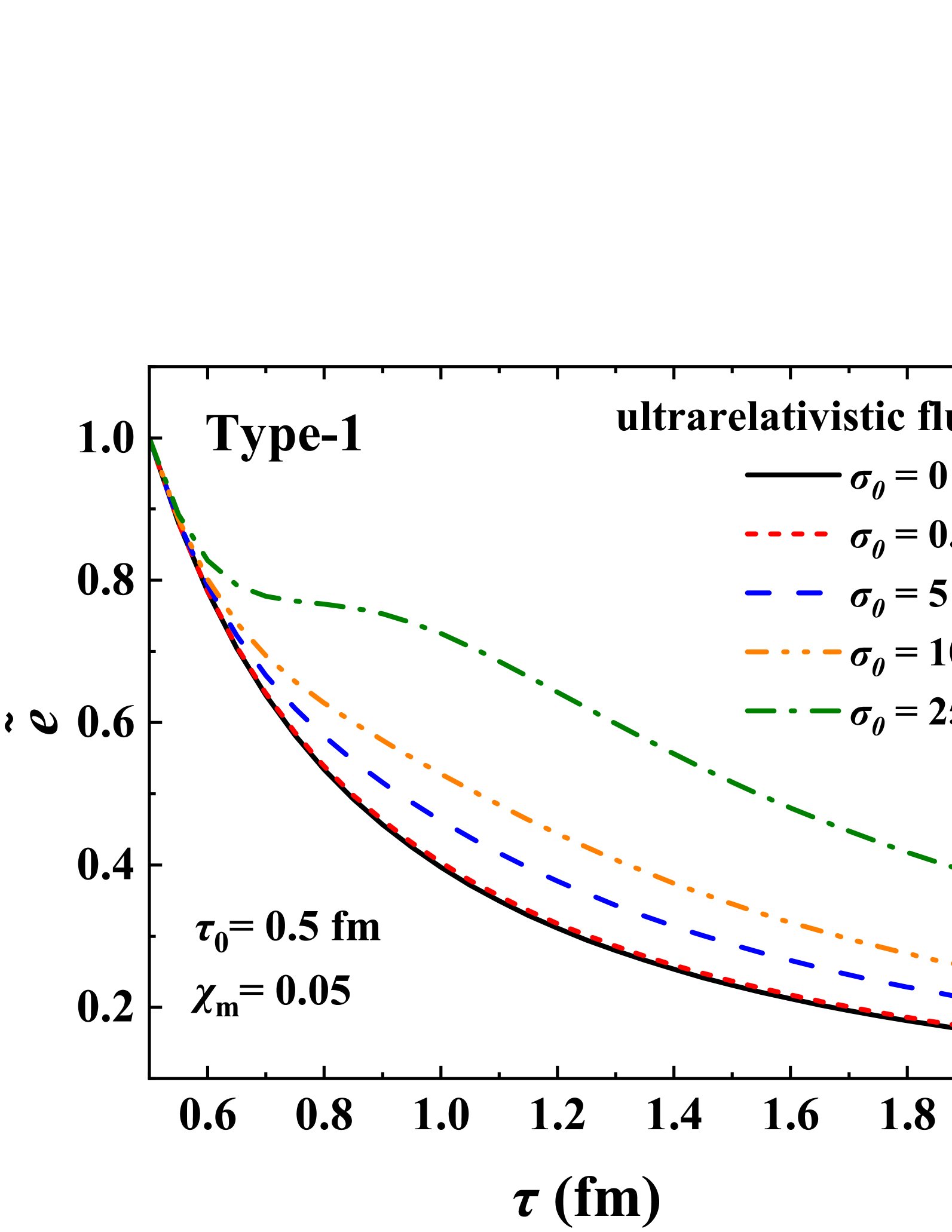
Figure 1: Evolution of energy density in the ultra-relativistic fluid. We choose magnetic susceptibility $\chi_{m}$ = 0.05. The left, middle, and right panels correspond to three different temporal evolution models of the magnetic field. The black solid line represents the case without a magnetic field. The red short dashed line, blue long dashed line, orange dash-dot-dotted line, and green dash-dotted line correspond to different values of $\sigma_{0}$ = 0.5, 5, 10 and 25, respectively.

IV.2 Magnetized Conformal Fluid

In this case, the energy density takes into account the degree of magnetization or the strength of the magnetic field, i.e., a conformal fluid with a magnetic field present in four-dimensional spacetime

$$e=\frac{1}{c_{s}^{2}}p-2MB.$$ (28)

Then, the conservation equation under different magnetic field models becomes

Type-1:

$$\partial_{\tau}\tilde{e}+\left(1+c_{s}^{2}\right)\frac{\tilde{e}}{\tau}+\frac{2\chi_{m}\sigma_{0}}{\left[1+\left(\tau-\tau_{0}\right)^{2}/\tau_{B}^{2}\right]^{2}}\left(\frac{c_{s}^{2}}{\tau}-\frac{\tau-\tau_{0}}{\left[1+\left(\tau-\tau_{0}\right)^{2}/\tau_{B}^{2}\right]\tau_{B}^{2}}\right)=0,$$ (29)

Type-2:

$$\partial_{\tau}\tilde{e}+\left(1+c_{s}^{2}\right)\frac{\tilde{e}}{\tau}+\chi_{m}\sigma_{0}\left(\frac{2c_{s}^{2}}{\tau\left[1+\left(\tau-\tau_{0}\right)^{2}/\tau_{B}^{2}\right]^{2}}-\frac{3(\tau-\tau_{0})\tau_{B}^{6}}{\left(\tau^{2}-2\tau\tau_{0}+\tau_{0}^{2}+\tau_{B}^{2}\right)^{4}}\right)=0,$$ (30)

Type-3:

$$\partial_{\tau}\tilde{e}+\left(1+c_{s}^{2}\right)\frac{\tilde{e}}{\tau}+\chi_{m}\sigma_{0}e^{-\frac{2|\tau-\tau_{0}|}{\tau_{B}}}\left(\frac{2c_{s}^{2}}{\tau}-\frac{1}{\tau_{B}}\frac{\partial|\tau-\tau_{0}|}{\partial\tau}\right)=0.$$ (31)

Figure 2 illustrates the effect of different magnetic field parameters on the evolution of energy density with proper time in the magnetized conformal fluid model, with the magnetic susceptibility $\chi_{m}$ fixed at 0.05. Figure 2 illustrates that stronger magnetic fields (higher $\sigma_{0}$) significantly slow the decay of energy density over proper time ($\tau$). For instance, the energy density for $\sigma_{0}=25$ (green dash-dotted line) decays much more slowly compared to weaker fields (e.g., $\sigma_{0}$ = 0.5, red short dashed line). This suppression arises due to magnetic pressure and Lorentz forces, which counteract the hydrodynamic expansion of the quark-gluon plasma (QGP). The magnetic field acts as a “brake” on energy dissipation by altering the fluid’s equation of state and flow dynamics.

The three magnetic field evolution models in relativistic heavy-ion collisions exhibit distinct trends: Type-1 causes the strongest suppression of energy density decay. Type-2 shows rapid early-stage energy dissipation for weak fields ($\sigma_{0}$ = 0.5), diverging from monotonic trends. Type-3 has the weakest overall impact on energy density evolution. These differences stem from the functional forms of the magnetic field decay (e.g., exponential vs. power-law dependence on $\tau$), which govern how magnetic energy is transferred to or stored in the fluid.

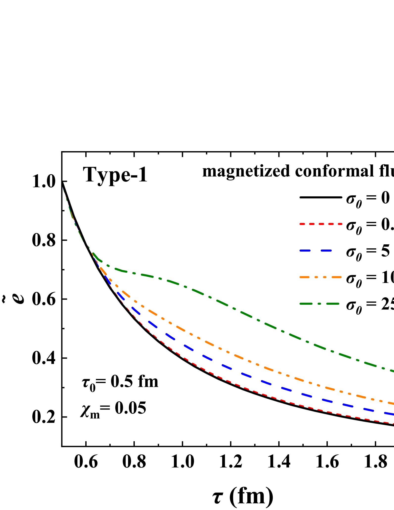
Figure 2: Evolution of energy density in the magnetized conformal fluid case. We choose $\chi_{m}$ = 0.05. The left, middle, and right panels correspond to Type-1, Type-2, and Type-3 magnetic field time evolution, respectively. The black solid line represents the case without a magnetic field. The red short dashed line, blue long dashed line, orange dash-dot-dotted line, and green dash-dotted line correspond to $\sigma_{0}$ = 0.5, 5, 10 and 25, respectively.

Figure 3 compares the normalized energy density evolution $\tilde{e}(\tau)$ between an ultra-relativistic fluid (blue dashed line) and a magnetized conformal fluid (red dotted line) under identical initial conditions ($\sigma_{0}$ = 25, $\chi_{m}$ = 0.05). Key insights include:

1. Fluid-Type Comparison: (i). The ultra-relativistic fluid exhibits faster energy dissipation due to its simplified equation of state ($p=c_{s}^{2}e$, $c_{s}^{2}=1/3$); (ii). The magnetized conformal fluid retains energy longer, as magnetization explicitly modifies the equation of state, introducing magnetic pressure and susceptibility effects.

2. Model Hierarchy: Suppression magnitude follows Type-1 $>$ Type-2 $>$ Type-3, consistent with Figs. 1 and 2.

3. Mechanistic Basis: Magnetic fields counteract hydrodynamic expansion via Lorentz forces, while susceptibility ($\chi_{m}$) enhances energy retention in the conformal fluid.

The slower energy decay in the magnetized conform fluids implies prolonged thermalization and altered freeze-out dynamics in the quark-gluon plasma (QGP). This could influence experimental observables such as anisotropic flow and particle spectra. The distinction between fluid types highlights the importance of incorporating magnetization into the equation of state for realistic QGP modeling.

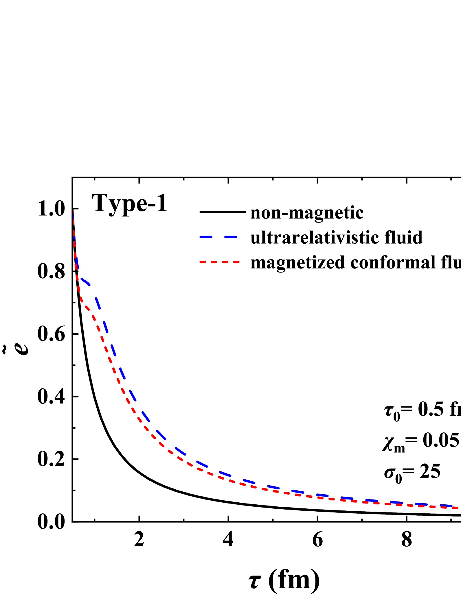
Figure 3: Evolution of the normalized energy density. The left, middle, and right panels correspond to Type-1, Type-2, and Type-3 magnetic field time evolution, respectively. The magnetic field parameter is set to $\sigma_{0}$ = 25, and the magnetic susceptibility is $\chi_{m}$ = 0.05. The black line, the blue dashed line and red dotted line correspond to the non-magnetic fluid, ultra-relativistic fluid and the magnetized conformal fluid, respectively.

V Energy-density evolution with temperature-dependent magnetic susceptibility

Following the rather “physical” discussion in the previous section, we now consider a more realistic scenario based on lattice QCD. For simplicity, we choose the temperature $T$ as the independent variable and express the magnetic susceptibility $\chi_{m}$ as a function of $T$. In lattice QCD calculations, the behavior of magnetic susceptibility as a function of temperature has been investigated using several different approaches (see, for example, Refs.Levkova and DeTar (2014); Bonati et al. (2014b); Bali et al. (2014b)). The latest lattice QCD results on the magnetic susceptibility $\chi_{m}$ of QCD matter, which can be found in Ref. Bali et al. (2020), show that at high temperatures, $\chi_{m}$ is parameterized in accordance with perturbative theory as follows

$$\chi_{m}(T)=2\beta_{1}\log\left(\frac{t}{q_{0}}\right)\frac{1+g_{0}/t+g_{1}/t^{2}+g_{2}/t^{3}}{1+g_{3}/t+g_{4}/t^{2}+g_{5}/t^{3}}e^{\left(-\frac{h_{3}}{t}\right)},$$ (32)

where $\beta_{1}=1/(6\pi^{2})$, $t$ parameter is defined as $T/1GeV$ ($T$ is the temperature), which shown as a dimensionless quantity. These parameters $q_{0}$, $g_{0}$, $g_{1}$, $g_{2}$, $g_{3}$, $g_{4}$, $g_{5}$ and $h_{3}$ are 0.1544, 23.99, -2.085, 0.1290, 21.35, -6.201, 0.5766 and 0.1497Bali et al. (2020), respectively.

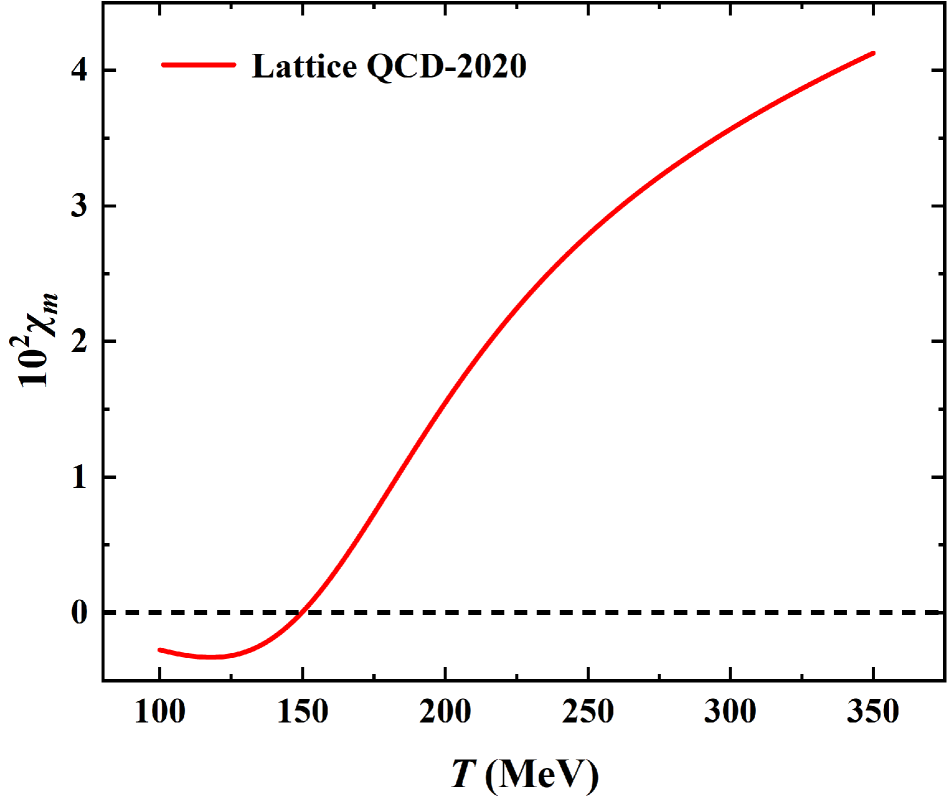
Figure 4: The magnetic susceptibility $\chi_{m}$ of QCD matter as a function of temperature. Results from lattice QCD calculations in 2020 (labeled as Lattice QCD-2020Bali et al. (2020)).

Figure 4 presents the magnetic susceptibility $\chi_{m}$ of QCD matter as a function of temperature, derived from lattice QCD calculations conducted in 2020Bali et al. (2020). The graph illustrates a significant increase in $\chi_{m}$ with rising temperature, transitioning from near-zero values at lower temperatures (approximately 100-150 MeV) to a steep ascent beyond 150 MeV. This trend suggests a marked change in the magnetic response of QCD matter as it transitions from hadronic to quark-gluon plasma (QGP) phases. In the confined phase, characterized by hadrons, the medium exhibits diamagnetic properties, with $\chi_{m}$, indicating a tendency to expel magnetic fields. Conversely, in the deconfined QGP phase, the medium becomes paramagnetic, with $\chi_{m}$, showing an increased magnetic response. Such temperature-dependent behavior is crucial for understanding the electromagnetic properties of QCD matter under extreme conditions, which is pertinent to the study of high-energy heavy-ion collisions and the evolution of early universe. The results from the lattice QCD-2020 calculations provide a valuable theoretical foundation for exploring the magnetic characteristics of QCD matter and their implications in high-energy physics, particularly in the context of phase transitions and the associated changes in magnetic susceptibility. Additionally, we introduce the parameter $k_{s}^{2}$ as

$$k_{s}^{2}(T)=\frac{p(T)}{e(T)}.$$ (33)

From the parameterization of s95n-v1 in the Ref. Huovinen and Petreczky (2010), it is known that

$$p(T)=T^{4}\int_{T_{1}}^{T}\frac{\theta(T^{\prime})}{T^{\prime 5}}\,dT^{\prime},$$ (34)

where $T_{1}=1$ MeV and the trace anomaly is given as

$$\theta(T)=T^{4}\left(\frac{d_{2}}{T^{2}}+\frac{d_{4}}{T^{4}}+\frac{c_{1}}{T^{n_{1}}}+\frac{c_{2}}{T^{n_{2}}}\right),$$ (35)

for $T\geq T_{0}$ ($T_{0}$ = 171.8 MeV), $n_{1}$, $n_{2}$, $d_{2}$, $d_{4}$, $c_{1}$, $c_{2}$ are 8, 9, $2.654\times 10^{4}~\text{GeV}^{2},6.563\times 10^{3}~\text{GeV}^{4},-4.370\times 10^{5}~\text{GeV}^{8},5.774\times 10^{6}~\text{GeV}^{9}$, respectively. For $T<T_{0}$ ($T_{0}$ = 171.8 MeV), the trace anomaly is given as

$$\theta(T)=T^{4}(a_{1}T+a_{2}T^{3}+a_{3}T^{4}+a_{4}T^{10}),$$ (36)

where $a_{1}$, $a_{2}$, $a_{3}$, $a_{4}$ are 4.654 GeV^-1, -879 GeV^-3, 8081 GeV⁴, -703900 GeV^-10Huovinen and Petreczky (2010), respectively.

The square of the sound speed $c_{s}^{2}$ as a function of temperature $T$ is obtained from the s95n-v1 parameterization in Ref.Huovinen and Petreczky (2010).

$$c_{s}^{2}=\frac{s}{T}\frac{dT}{ds},$$ (37)

where entropy density $s=(4p+\theta)/T$ is computed from the trace anomaly and Eq.(34). $k_{s}^{2}(T)$ is obtained from Eq. (33).

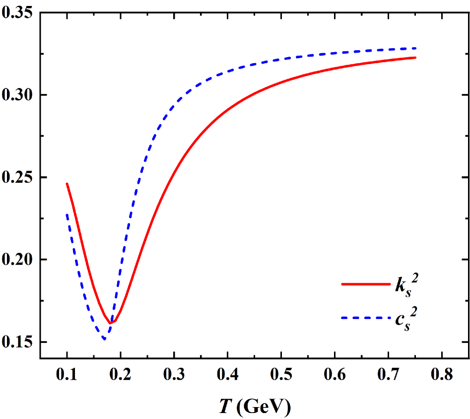
Figure 5: Behavior of $k_{s}^{2}(T)=p(T)/e(T)$ and of $c_{s}^{2}(T)$. The blue dashed line represents the sound speed parameterization derived from the equation, while the red solid line provides the ratio between pressure and energy densityHuovinen and Petreczky (2010).).

Figure 5 illustrates the behavior of $k_{s}^{2}$ and $c_{s}^{2}$ as functions of temperature $T$, revealing a close similarity between the two. At lower temperatures (around $T<0.2$ GeV), both $k_{s}^{2}$ and $c_{s}^{2}$ are relatively small. Specifically, $c_{s}^{2}$ shows a significant downward trend, reaching a local minimum within this temperature range. As the temperature increases further, $c_{s}^{2}$ begins to rise from its local minimum and intersects with $k_{s}^{2}$ at around $T$ = 0.2 GeV. At higher temperature conditions, both $k_{s}^{2}$ and $c_{s}^{2}$ continue to increase. However, $c_{s}^{2}$ grows at a relatively faster rate, causing its value to gradually surpass $k_{s}^{2}$. As the temperature continues to rise, the variation of both approaches a steady trend, suggesting that the system may have reached a certain equilibrium state at high temperatures. When assuming $B/s$ is a conserved quantity, the Eq. (16) is satisfied. When assuming the dependence of magnetic field on proper time $\tau$, one can obtain the energy density as

$$e=\frac{Ts}{1+k_{s}^{2}}=\frac{Ts_{0}}{\left(1+k_{s}^{2}\right)\left[1+(\tau-\tau_{0})^{2}/\tau_{B}^{2}\right]^{3/2}},$$ (38)

then substituting it into the differential Eq. (26), one obtains

$$\begin{split}0=&\,\partial_{\tau}\left[\frac{T}{\left[1+\left(\tau-\tau_{0}\right)^{2}/\tau_{B}^{2}\right]^{3/2}\left(1+k_{s}^{2}(T(\tau))\right)}\right]\\ &+\frac{T}{\left[1+\left(\tau-\tau_{0}\right)^{2}/\tau_{B}^{2}\right]^{3/2}\tau}-\frac{3\chi_{m}\sigma_{0}(\tau-\tau_{0})\tau_{B}^{6}}{\left(\tau^{2}-2\tau\tau_{0}+\tau_{0}^{2}+\tau_{B}^{2}\right)^{4}}\frac{1}{1+k_{s}^{2}(T_{0})},\end{split}$$ (39)

upon solving the equation, the normalized energy density can be obtained as

$$\tilde{e}=\frac{e(\tau)}{e_{0}}=\frac{1}{\left[1+\left(\tau-\tau_{0}\right)^{2}/\tau_{B}^{2}\right]^{3/2}}\frac{T(\tau)}{T_{0}}\frac{1+k_{s}^{2}(T_{0})}{1+k_{s}^{2}(T(\tau))}.$$ (40)

Figure 6 illustrates the normalized energy density $\tilde{e}(\tau)$ as a function of proper time $\tau$ in the confined quark-gluon plasma (QGP) phase, incorporating a temperature-dependent magnetic susceptibility $\chi_{m}(T)$ derived from lattice QCD. The initial temperature is set to $T_{0}$ = 200 MeV, and the results are compared for different initial magnetic field strengths ($\sigma_{0}=B_{0}^{2}/e_{0}$ = 5, 10 and 25).

Figure 6 demonstrates that stronger magnetic fields significantly slow down the decay of energy density over time. For instance, the green dash-dotted line ($\sigma_{0}$ = 25) shows a much slower dissipation compared to weaker fields ($\sigma_{0}=5$) and the non-magnetized case (black solid line).

The results align with the paramagnetic behavior of the QGP phase ($\chi_{m}(T)>0$), where the medium enhances its magnetic response at high temperatures. The temperature-dependent $\chi_{m}(T)$ captures the transition from diamagnetism ($\chi_{m}(T)<0$) in the confined hadronic phase to paramagnetism ($\chi_{m}(T)>0$) in the deconfined QGP phase, reflecting the QCD phase structure’s influence on electromagnetic properties. Previous studies (e.g., Figs. 1, 2, 3) assumed a constant $\chi_{m}$, oversimplifying the QGP’s magnetic response. By adopting lattice QCD-based $\chi_{m}(T)$, this work accounts for the temperature-driven phase transition in QCD matter, making the model more consistent with first-principles calculations. The inclusion of $\chi_{m}(T)$ explicitly links the QGP’s electromagnetic properties to its thermodynamic state. Temperature-dependent $\chi_{m}(T)$ introduces a feedback loop between the fluid’s thermal evolution and its electromagnetic properties. For example, slower energy dissipation (due to strong fields) maintains higher temperatures, sustaining paramagnetic behavior and further influencing field evolution.

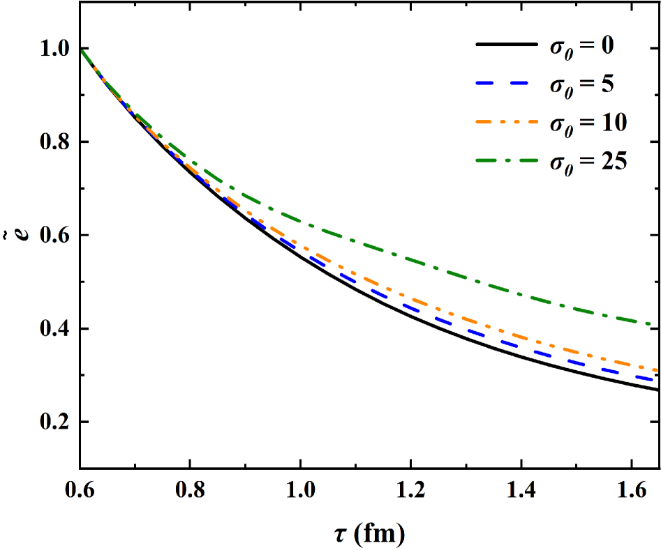
Figure 6: The dependence of normalized energy density on proper time. An initial temperature $T_{0}$ = 200 MeV and an initial time $\tau_{0}=0.6\textrm{fm/c}$ are set. The black solid line represents the case without magnetic field. The blue dashed line, orange dash-dot-dotted line, and green dash-dotted line correspond to different values of $\sigma_{0}$ = 5, 10, and 25, respectively.).

The use of lattice QCD-derived $\chi_{m}(T)$ represents a significant step toward realistic modeling of magnetized QGP. It bridges theoretical predictions with experimental conditions in heavy-ion collisions and opens avenues for exploring the QCD phase diagram’s electromagnetic signatures. By incorporating dynamic magnetic responses, this work paves the way for deeper insights into the interplay between quantum chromodynamics and relativistic magnetohydrodynamics.

VI Summary and Conclusions

In this work, we systematically investigated the evolution of energy density in relativistic fluids under time-dependent magnetic fields within the framework of relativistic magnetohydrodynamics (RMHD). By incorporating three distinct magnetic field evolution models (Type-1, Type-2, and Type-3) in relativistic heavy-ion collisions (RHIC) into the Bjorken flow framework, we analyzed their impacts on energy dissipation dynamics in both ultra-relativistic and magnetized conformal fluids. Furthermore, a temperature-dependent magnetic susceptibility derived from lattice QCD calculations was introduced to enhance the physical realism of the magnetic response in quark-gluon plasma (QGP). Our results demonstrate that magnetic fields play a critical role in modulating energy dissipation. Stronger magnetic fields consistently suppress the decay of energy density across all models, with the suppression magnitude being model-dependent. Notably, Type-1 exhibits the most pronounced retardation of energy dissipation, while Type-3 shows the weakest effect. This divergence arises from the distinct temporal evolution profiles of the magnetic fields, which govern how magnetic energy couples to the fluid. For instance, in ultra-relativistic fluids, the interplay between magnetic pressure and hydrodynamic expansion leads to slower thermalization, while in magnetized conformal fluids, explicit magnetization terms in the equation of state amplify energy retention.

The inclusion of temperature-dependent magnetic susceptibility further enriches the dynamics. Lattice QCD-based parametrizations reveal a transition from diamagnetic behavior in the confined phase to paramagnetic response in the deconfined QGP phase. This temperature dependence introduces a feedback mechanism: delayed energy dissipation sustains higher temperatures, reinforcing paramagnetic behavior and influencing the magnetic field evolution. Such findings underscore the necessity of integrating QCD-based susceptibilities into RMHD frameworks for accurate modeling of heavy-ion collisions.

This study bridges theoretical RMHD models with experimental observables, emphasizing the importance of precise magnetic field modeling in interpreting QGP dynamics. However, several limitations warrant future exploration. First, dissipative effects such as viscosity and finite conductivity neglected in the ideal MHD approximation could modify energy-momentum transfer. In conclusion, our work advances the understanding of magnetized QGP evolution by highlighting the interplay between magnetic field dynamics, QCD phase structure, and hydrodynamic expansion. These insights pave the way for more sophisticated RMHD simulations that incorporate realistic electromagnetic properties, ultimately enhancing our ability to decode the complex physics of high-energy nuclear matter.

References

References

- Adams et al. (2005) J. Adams et al., Nucl. Phys. A 757, 102 (2005).
- Gyulassy and McLerran (2005) M. Gyulassy and L. McLerran, Nucl. Phys. A 750, 30 (2005).
- Heinz and Kolb (2002) U. W. Heinz and P. F. Kolb, Nucl. Phys. A 702, 269 (2002).
- Hirano et al. (2006) T. Hirano, U. W. Heinz, D. Kharzeev, R. Lacey, and Y. Nara, Phys. Lett. B 636, 299 (2006).
- Guo et al. (1999) L. B. Guo, L. S. Liu, and D. S. Du, J. Phys. G 25, 1 (1999).
- Moreland et al. (2015) J. S. Moreland, J. E. Bernhard, and S. A. Bass, Phys. Rev. C 92, 011901 (2015).
- Shuryak (2004) E. Shuryak, Prog. Part. Nucl. Phys. 53, 273 (2004).
- Heinz and Snellings (2013) U. Heinz and R. Snellings, Ann. Rev. Nucl. Part. Sci. 63, 123 (2013).
- Bzdak and Skokov (2012) A. Bzdak and V. Skokov, Phys. Lett. B 710, 171 (2012).
- Deng and Huang (2012) W.-T. Deng and X.-G. Huang, Phys. Rev. C 85, 044907 (2012).
- Tuchin (2013) K. Tuchin, Adv. High Energy Phys. 2013, 490495 (2013).
- Mo et al. (2013) Y.-J. Mo, S.-Q. Feng, and Y.-F. Shi, Phys. Rev. C 88, 024901 (2013).
- Zhong et al. (2014) Y. Zhong, C.-B. Yang, X. Cai, and S.-Q. Feng, Adv. High Energy Phys. 2014, 193039 (2014).
- Zhong et al. (2015) Y. Zhong, C.-B. Yang, X. Cai, and S.-Q. Feng, Chin. Phys. C 39, 104105 (2015).
- Roy and Pu (2015) V. Roy and S. Pu, Phys. Rev. C 92, 064902 (2015).
- Li et al. (2016) H. Li, X.-l. Sheng, and Q. Wang, Phys. Rev. C 94, 044903 (2016).
- Kharzeev et al. (2008) D. E. Kharzeev, L. D. McLerran, and H. J. Warringa, Nucl. Phys. A 803, 227 (2008).
- She et al. (2018) D. She, S.-Q. Feng, Y. Zhong, and Z.-B. Yin, Eur. Phys. J. A 54, 48 (2018).
- Chen and Feng (2020) B.-X. Chen and S.-Q. Feng, Chin. Phys. C 44, 024104 (2020).
- Chen et al. (2021) Y. Chen, X.-L. Sheng, and G.-L. Ma, Nucl. Phys. A 1011, 122199 (2021).
- Kharzeev and Warringa (2009) D. E. Kharzeev and H. J. Warringa, Phys. Rev. D 80, 034028 (2009).
- Fukushima et al. (2008) K. Fukushima, D. E. Kharzeev, and H. J. Warringa, Phys. Rev. D 78, 074033 (2008).
- Guo et al. (2019) Y. Guo, S. Shi, S. Feng, and J. Liao, Phys. Lett. B 798, 134929 (2019).
- Aghababaie and Burgess (2004) Y. Aghababaie and C. P. Burgess, Phys. Rev. D 70, 085003 (2004).
- Kharzeev and Yee (2011) D. E. Kharzeev and H.-U. Yee, Phys. Rev. D 83, 085007 (2011).
- Burnier et al. (2011) Y. Burnier, D. E. Kharzeev, J. Liao, and H.-U. Yee, Phys. Rev. Lett. 107, 052303 (2011).
- Jiang et al. (2024) Z.-F. Jiang, Z.-H. Zhang, X.-F. Yuan, and B.-W. Zhang, Phys. Rev. C 110, 014902 (2024).
- Khachatryan et al. (2017) V. Khachatryan et al. (CMS), Phys. Rev. Lett. 118, 122301 (2017).
- Sirunyan et al. (2018) A. M. Sirunyan et al. (CMS), Phys. Rev. C 97, 044912 (2018).
- Sirunyan et al. (2019) A. M. Sirunyan et al. (CMS), Phys. Rev. C 100, 064908 (2019).
- Qiu and Feng (2023) Y.-W. Qiu and S.-Q. Feng, Phys. Rev. D 107, 076004 (2023).
- Zhu and Feng (2023) X. Zhu and S.-Q. Feng, Phys. Rev. D 107, 016018 (2023).
- Deng and Feng (2022) J. Deng and S.-Q. Feng, Phys. Rev. D 105, 026015 (2022).
- Qiu et al. (2023) Y.-W. Qiu, S.-Q. Feng, and X.-Q. Zhu, Phys. Rev. D 108, 116022 (2023).
- Bao and Feng (2024) Y.-R. Bao and S.-Q. Feng, Phys. Rev. D 109, 096033 (2024).
- Feng et al. (2020) S.-Q. Feng, Y.-Q. Zhao, and X. Chen, Phys. Rev. D 101, 026023 (2020).
- Zhu et al. (2019) Z.-R. Zhu, S.-Q. Feng, Y.-F. Shi, and Y. Zhong, Phys. Rev. D 99, 126001 (2019).
- Feng et al. (2018) S.-Q. Feng, L. Pei, F. Sun, Y. Zhong, and Z.-B. Yin, Chin. Phys. C 42, 054102 (2018).
- Bjorken (1983) J. D. Bjorken, Phys. Rev. D 27, 140 (1983).
- Müller and Schäfer (2018) B. Müller and A. Schäfer, Phys. Rev. D 98, 071902 (2018).
- Jiang et al. (2018) Y. Jiang, S. Shi, Y. Yin, and J. Liao, Chin. Phys. C , 011001 (2018).
- Shi et al. (2018) S. Shi, Y. Jiang, E. Lilleskov, and J. Liao, Annals Phys. 394, 50 (2018).
- Bali et al. (2014a) G. S. Bali, F. Bruckmann, G. Endrodi, and A. Schafer, Phys. Rev. Lett. 112, 042301 (2014a).
- Bonati et al. (2013) C. Bonati, M. D’Elia, M. Mariti, F. Negro, and F. Sanfilippo, Phys. Rev. Lett. 111, 182001 (2013).
- Bonati et al. (2014a) C. Bonati, F. Capponi, M. D’Elia, and F. Negro, PoS LATTICE2013, 135 (2014a).
- Levkova and DeTar (2014) L. Levkova and C. DeTar, Phys. Rev. Lett. 112, 012002 (2014).
- Bonati et al. (2014b) C. Bonati, M. D’Elia, M. Mariti, F. Negro, and F. Sanfilippo, Phys. Rev. D 89, 054506 (2014b).
- Simonov and Orlovsky (2015) Y. A. Simonov and V. D. Orlovsky, JETP Lett. 101, 423 (2015).
- Bali et al. (2014b) G. S. Bali, F. Bruckmann, G. Endrödi, S. D. Katz, and A. Schäfer, JHEP 08, 177 (2014b).
- Pu et al. (2016) S. Pu, V. Roy, L. Rezzolla, and D. H. Rischke, Phys. Rev. D 93, 074022 (2016).
- Li and Yee (2018) S. Li and H.-U. Yee, Phys. Rev. D 97, 056024 (2018).
- Jaiswal et al. (2019) S. Jaiswal, C. Chattopadhyay, A. Jaiswal, S. Pal, and U. Heinz, Phys. Rev. C 100, 034901 (2019).
- Jaiswal et al. (2022) S. Jaiswal, C. Chattopadhyay, L. Du, U. Heinz, and S. Pal, Phys. Rev. C 105, 024911 (2022).
- Karimabadi et al. (2023) M. Karimabadi, A. F. Kord, and B. Azadegan, Nucl. Phys. A 1040, 122748 (2023).
- Caldarelli et al. (2009) M. M. Caldarelli, O. J. C. Dias, and D. Klemm, JHEP 03, 025 (2009).
- Huang et al. (2010) X.-G. Huang, M. Huang, D. H. Rischke, and A. Sedrakian, Phys. Rev. D 81, 045015 (2010).
- Kamikado and Kanazawa (2015) K. Kamikado and T. Kanazawa, JHEP 01, 129 (2015).
- Bergman et al. (2008) O. Bergman, G. Lifschytz, and M. Lippert, JHEP 05, 007 (2008).
- Cherman et al. (2009) A. Cherman, T. D. Cohen, and E. S. Werbos, Phys. Rev. C 79, 045203 (2009).
- Steinert and Cassing (2014) T. Steinert and W. Cassing, Phys. Rev. C 89, 035203 (2014).
- Kabat et al. (2002) D. N. Kabat, K.-M. Lee, and E. J. Weinberg, Phys. Rev. D 66, 014004 (2002).
- Anber and Ünsal (2014) M. M. Anber and M. Ünsal, JHEP 12, 107 (2014).
- Tawfik and Magdy (2014) A. N. Tawfik and N. Magdy, Phys. Rev. C 90, 015204 (2014).
- Bali et al. (2020) G. S. Bali, G. Endrödi, and S. Piemonte, JHEP 07, 183 (2020).
- Huovinen and Petreczky (2010) P. Huovinen and P. Petreczky, Nucl. Phys. A 837, 26 (2010).