From Interpretation to Correction: A Decentralized Optimization Framework for Exact Convergence in Federated Learning

Abstract

This work introduces a novel decentralized framework to interpret federated learning (FL) and, consequently, correct the biases introduced by arbitrary client participation and data heterogeneity, which are two typical traits in practical FL. Specifically, we first reformulate the core processes of FedAvg – client participation, local updating, and model aggregation – as stochastic matrix multiplications. This reformulation allows us to interpret FedAvg as a decentralized algorithm. Leveraging the decentralized optimization framework, we are able to provide a concise analysis to quantify the impact of arbitrary client participation and data heterogeneity on FedAvg’s convergence point. This insight motivates the development of Federated Optimization with Exact Convergence via Push-pull Strategy ( FOCUS ), a novel algorithm inspired by decentralized algorithm that eliminates these biases and achieves exact convergence without requiring the bounded heterogeneity assumption. Furthermore, we theoretically prove that FOCUS exhibits linear convergence (exponential decay) for both strongly convex and non-convex functions satisfying the Polyak-Lojasiewicz condition, regardless of the arbitrary nature of client participation.

1 Introduction

While federated learning (FL) has demonstrated considerable success in practical applications, it encounters a fundamental challenge in its inability to achieve exact convergence under arbitrary client participation using a constant learning rate (Karimireddy et al., 2020; Wang and Ji, 2022). To interpret this, recall the goal of the FL problem is to minimize the following loss function:

$$F(x):=\frac{1}{N}\sum_{n=1}^{N}f_{n}(x),\;\;\;f_{n}(x):=\mathbb{E}\hskip 1.42271pt_{\xi\sim{\mathcal{D}}_{n}}\hat{f}_{n}(x;\xi),$$ (1)

where $x\in^{d}$ represents the $d$-dimensional model parameter, and the local objective function $f_{n}(x)$ is defined as an expected loss function w.r.t. a client’s local private data distribution $D_{n}$. Almost all existing FL works incorporate two techniques: partial client participation and multiple local updates, which is known to lead to inexact convergence (McMahan et al., 2017; Stich, 2018; Kairouz et al., 2021). 1) Unless the impractical uniform participation assumption, arbitrary client participation, i.e., clients may participate with any unknown probability, will result in the FL algorithm converging to a stationary point of a weighted loss function that is different from the original loss function (Wang and Ji, 2022). 2) Multiple local updates can lead to client drift due to data heterogeneity across clients (Karimireddy et al., 2020). It means that clients’ local models may significantly diverge from the global model at the server, which impedes the FL algorithm’s convergence to the stationary point of (1) (Li et al., 2019a, 2020). Hence, we raise a crucial question:

We will provide a positive answer to this question in this paper. To achieve that, we introduce a novel FL algorithm called FOCUS that departs from the heuristic modifications commonly applied to existing algorithms. Instead, our FOCUS draws from the principles of decentralized optimization algorithms (Nedic and Ozdaglar, 2009; Sayed et al., 2014; Lian et al., 2017; Lan et al., 2020), offering a fundamentally different perspective.

As we will explain in detail in the next section, FL algorithms and decentralized algorithms are known to be closely related, but not much work is dedicated to systematically describing them in a unified framework. To bridge the gap between decentralized learning and FL, we frame the process using graph theory and stochastic matrices. By modeling client participation, local updates, and model aggregation as a sequence of stochastic matrix multiplications, we establish a formal connection between the two paradigms. This framework allows us to leverage powerful established theorems from decentralized optimization to simultaneously tackle the dual challenges of arbitrary client participation and local updates. Ultimately, our approach provides a rigorous foundation for analyzing and enhancing FL algorithms. Lastly, this work focuses quite differently from the decentralized FL work (Beltrán et al., 2023; Shi et al., 2023; Fang et al., 2024), which is more closely related to decentralized algorithms instead of FL.

Our main contributions are summarized as follows:

• We provide a systematic approach to reformulate all core processes of FL – client participation, local updating, and model aggregation.

• By reformulating FedAvg as a decentralized algorithm, we offer a concise analysis that quantifies the bias of its limiting point under arbitrary client participation.

• We propose Federated Optimization with Exact Convergence via Push-pull Strategy ( FOCUS ), which converges to the exact solution under arbitrary client participation without assuming the bounded heterogeneity.

• Even under arbitrary client participation, FOCUS exhibits linear convergence (exponential decay) for both convex and non-convex (with PL condition) scenarios.

• We also introduce a stochastic gradient variant, SG-FOCUS , which demonstrates faster convergence and higher accuracy, both theoretically and empirically.

2 Related Work and Review: Federated Learning and Decentralized Algorithms

It is known that federated learning (FL) and decentralized optimization algorithms are closely related (Lalitha et al., 2018; Koloskova et al., 2020; Kairouz et al., 2021). However, the two fields emphasize different aspects and employ slightly different terminology. We begin with a brief overview of the two most representative algorithms, FedAvg and DGD, along with the related works.

2.1 Federated Learning Algorithm Review

FedAvg (McMahan et al., 2017) is the most widely adopted algorithm in FL. It roughly consists of three steps: 1) the server activates a subset of clients, which then retrieves the server’s current model. 2) Each activated client independently updates the model by training on its local dataset. 3) Finally, the server aggregates the updated models received from the clients, computing their average. This process can be represented mathematically as:

$$x_{r,i}^{1}=x_{r},\;\;\forall i\in S_{r}$$ (Pull Model)

$$\mbox{{For}\; }k=0,1,\cdots,\tau-1:$$ (Local Update)

$$\hskip 14.22636ptx_{r,i}^{k+1}=x_{r,i}^{k}-\eta\nabla f_{i}(x_{r,i}^{k}) \;\;\forall i\in S_{r}\mbox{\; in parallel}$$

$$x_{r+1}=\frac{1}{|S_{r}|}\sum_{i\in S_{r}}x_{r,i}^{K+1}$$ (Aggregate Model)

where the set $S_{r}$ represents the indices of the sampled clients at the communication round $r$. The notation $x_{r}\in\mathbb{R}^{d}$ stands for the server’s model parameters at $r$-th round, while $x_{r,i}^{k}$ stands for the client $i$’s model at the $k$-th local update step in the $r$-th round.

Because of the data heterogeneity and multiple local update steps, Li et al. (2019a) has shown that the fixed point of FedAvg is not the same as the minimizer of (1) in the convex scenario. More specifically, they quantified that

$$\|x^{o}-x^{\star}\|^{2}=\Omega\big{(}(\tau-1)\eta\big{)}\|x^{\star}\|^{2},$$ (3)

where $x^{o}$ is the fixed point of the FedAvg algorithm and $x^{\star}$ is the optimal point. This phenomenon, commonly referred to as client drift (Karimireddy et al., 2020), can be mitigated by introducing a control variate during the local update step, an approach inspired by variance reduction techniques (Johnson and Zhang, 2013). Prominent examples of this strategy, including SCAFFOLD (Karimireddy et al., 2020) and ProxSkip (Mishchenko et al., 2022), can further circumvent the need for a bounded heterogeneity assumption. Yet, this approach incurs increased communication costs, doubling it due to the transmission of a control variate with the same dimensionality as the model parameters.

2.1.1 Arbitrary Client Participation Modeling

Modeling the sampled client indices, denoted as $S_{r}$, is another crucial research area in FL. Many analytical studies on FL assume that $S_{r}$ is drawn from a uniform distribution, an assumption shared by the literature cited in the preceding paragraph, but this is almost impractical in reality (Kairouz et al., 2021; Xiang et al., 2024). Wang and Ji (2022) demonstrated that FedAvg might fail to converge to $x^{\star}$ under non-uniform sampling distributions, even with a decreasing learning rate $\eta$. To address the challenges posed by non-uniformity, a common approach involves either explicitly knowing or adaptively learning the client participation probabilities during the iterative process and subsequently modifying the averaging weights accordingly (Wang and Ji, 2023; Wang et al., 2024; Xiang et al., 2024). However, this approach is not inherently compatible with existing control variate methods. Instead, we will derive a natural solution for both data heterogeneity and non-uniform challenges using a decentralized algorithmic approach.

Inspired by (Wang and Ji, 2022), in this paper, we model the arbitrary client participation by the following assumption.

Assumption 1 (Arbitrary Client Participation)

In each communication round, the participation of the $i-$th worker is indicated by the event $\mathbb{I}_{i}$, which occurs with a unknown probability $p_{i}\in(0,1]$. $\mathbb{I}_{i}=1$ indicates that the $i$-th worker is activated while $\mathbb{I}_{i}=0$ indicates not. The corresponding averaging weights are denoted by $q_{i}$, where $q_{i}=\mathbb{E}\hskip 1.42271pt[\mathbb{I}_{i}/(\sum_{j=1}^{N}\mathbb{I}_{j})]$.

Assumption 1 is a general one covering multiple cases:

• Case 1: Full Client Participation. Although there is no randomness, it still can be modeled as $p_{i}\equiv 1$ and $q_{i}\equiv\frac{1}{N}$.

• Case 2: Active Arbitrary Participation.

• Each client $i$ independently determines if they will participate in the communication round. The event $\mathbb{I}_{i}$ follows the Bernoulli distribution $p_{i}$, where $p_{i}\in(0,1]$. (Note $\sum_{i}p_{i}\neq 1$.) If $\{p_{i}\}_{i=1}^{N}$ are close to each other, then $q_{i}\approx p_{i}/(\sum_{j}p_{j})$.

• Case 3: Passive Arbitrary Participation. The server randomly samples $m$ clients in each round. Each client is randomly selected without replacement according to the category distribution with the normalized weights $q_{1},q_{2},\cdots,q_{N}$, where $\sum_{i}q_{i}=1,q_{i}>0$. $p_{i}$ does not have a simple closed form. But if it is sampled with replacement, then $p_{i}=1-(1-q_{i})^{m}$.

• Case 3a: Uniform Sampling. This is a special case of case 3. In this case, $p_{i}=m/N$ and $q_{i}=1/m$ for all $i$.

Usually, the passive arbitrary participation also commonly refers to arbitrary client sampling. We also interactively use sampling and client participation in this paper.

2.2 Decentralized Algorithm Review

The most widely adopted decentralized algorithm is decentralized gradient descent (DGD) (Nedic and Ozdaglar, 2009; Yuan et al., 2016), along with its adapt-then-combine version diffusion algorithm (Cattivelli et al., 2008; Chen and Sayed, 2012). It is also a distributed algorithm where multiple workers collaboratively train a model without sharing local data. In contrast to FedAvg, DGD has three key distinctions. First, it operates without a central server; instead, workers communicate directly with their neighbors according to a predefined network topology (Nedic and Ozdaglar, 2009; Sayed et al., 2014; Lian et al., 2017). Second, rather than relying on a server for model aggregation, workers exchange and combine model parameters with their neighbors through linear combinations dictated by the network structure. This process can be formally expressed as

$$x_{k,i}^{+}= x_{k,i}-\eta\nabla f_{i}(x_{k,i})$$ (Local Update) (4)

$$x_{k+1,i}= \sum_{j\in\mathcal{N}_{i}}w_{i,j}x_{k,j}^{+}$$ (Graph Combination) (5)

where $x_{k,i}$ stands for the $i$-th worker’s parameters at the $k$-th iteration, the set $\mathcal{N}_{i}$ represents the neighbor’s indices of worker $i$, and the non-negative weights $w_{i,j}$ satisfy $\sum_{j\in\mathcal{N}_{i}}w_{i,j}=1$ for all $i$. Third, the algorithm is typically written as a single for-loop style instead of two-level for-loop representations. It is straightforward to incorporate the multi-local-update concept into decentralized algorithms. However, it is not popular in the decentralized community.

Figure 1: An illustration of Decentralized Gradient Descent.

It is well-known that the DGD with a fixed step size $\eta$ only converges to an ${\mathcal{O}}(\eta)$-sized neighborhood of the solution of the original algorithm (Yuan et al., 2016). This resembles the FedAvg algorithm exactly. Subsequently, several extract decentralized optimization algorithms have been proposed, such as Extra (Shi et al., 2015), exact-diffusion/NIDS (Yuan et al., 2018; Li et al., 2019b), DIGing/Gradient tracking (Nedic et al., 2017), etc. The key advancement of these algorithms is their capability to achieve extra convergence under a fixed step size. They formulate the original sum-of-cost problem into a constrained optimization problem and then apply the primal-dual style approach to solve the constrained problem (Ryu and Yin, 2022).

While it is common in the analysis of decentralized algorithms to assume a static and strongly connected underlying graph structure, a significant body of research also investigates time-varying graph topologies (Assran et al., 2019; Lan et al., 2020; Saadatniaki et al., 2020; Ying et al., 2021). These studies often adopt one of two common assumptions regarding the dynamics of such graphs: either the union of graphs over any consecutive $\tau-$ iterations or the expected graph is strongly connected (Nedić and Olshevsky, 2014; Koloskova et al., 2020). Whereas previous research on time-varying topologies often relies on specific graph assumptions, this paper takes a different approach. We model client sampling and local updates using a graph representation, thereby avoiding any presuppositions about the underlying graph structure.

$$R=\begin{bmatrix}1&0&0&0&0\\[1.42262pt] 1&0&0&0&0\\[1.42262pt] 0&0&1&0&0\\[1.42262pt] 1&0&0&0&0\\[1.42262pt] 0&0&0&0&1\end{bmatrix},\;V=\begin{bmatrix}0&\frac{1}{2}&0&\frac{1}{2}&0\\[1.42262pt] 0&1&0&0&0\\[1.42262pt] 0&0&1&0&0\\[1.42262pt] 0&0&0&1&0\\[1.42262pt] 0&0&0&0&1\end{bmatrix},\;C=\begin{bmatrix}1&1&0&1&0\\[1.42262pt] 0&0&0&0&0\\[1.42262pt] 0&0&1&0&0\\[1.42262pt] 0&0&0&0&0\\[1.42262pt] 0&0&0&0&1\end{bmatrix},\;W=\begin{bmatrix}\frac{1}{3}&\frac{1}{3}&0&\frac{1}{3}&0\\[1.42262pt] \frac{1}{3}&\frac{2}{3}&0&0&0\\[1.42262pt] 0&0&1&0&0\\[1.42262pt] \frac{1}{3}&0&0&\frac{2}{3}&0\\[1.42262pt] 0&0&0&0&1\end{bmatrix}.$$

Figure 2: The graph representation of the communication pattern of 5 nodes and its possible corresponding stochastic matrices. For clearness, the self-loop is not drawn. If the node 0 is treated as server and node 1 to 4 as clients, the left most is a typical pull-model step, i.e. client 1 and 3 are participated; the second left graph depicts the model average step in the FedAvg; the third graph is a same graph but using column-stochastic matrix, which is uncommon in the FL literature; The last one is a typical (symmetric) doubly stochastic matrix case used in the decentralized optimization algorithm.

Figure 3: Represent the Federated Learning in a decentralized framework. The dashed line means no communication.

3 Interpretation: Representing FL through Decentralized Algorithms

The power of decentralized algorithms is presented when they are expressed in matrix form. In this section, we will first reformulate FedAvg into a decentralized matrix form, then provide a new analysis for the arbitrary sampling case based on this form directly.

3.1 Reformulating FedAvg

DGD (4)-(5) is commonly written in a compact matrix form that captures the behavior of all workers

$${\boldsymbol{x}}_{k+1}= W({\boldsymbol{x}}_{k}-\eta\nabla{\boldsymbol{f}}({\boldsymbol{x}}_{k})),$$ (DGD matrix form)

where ${\boldsymbol{x}}_{k+1}={\rm vstack}[x_{k,1};x_{k,2};\cdots;x_{k,N}]\in\mathbb{R}^{N\times d}$ is a vertically stacked vector of all workers’ $x_{k,i}$ and

$$\nabla{\boldsymbol{f}}({\boldsymbol{x}}_{k})=\begin{bmatrix}{-}\nabla f_{1}(x_{k,1}){-}\\ \vdots\\ {-}\nabla f_{N}(x_{k,N}){-}\end{bmatrix}\in\mathbb{R}^{N\times d}$$ (6)

is the corresponding stacked local gradients; and $W=[w_{i,j}]_{i,j=1}^{N}\in\mathbb{R}^{N\times N}$ is called the mixing matrix, which typically plays a crucial role in decentralized algorithms.

Expressing FedAvg in this decentralized matrix form requires recognizing that the matrix-vector multiplication $Wx$ represents a specific communication pattern, and varying $W$ can result in a different interpretation of communication. Taking two concrete toy cases as examples:

$$W_{\rm assign}x= \begin{bmatrix}1&0&0\\ 1&0&0\\ 0&0&1\end{bmatrix}\begin{bmatrix}x_{0}\\ x_{1}\\ x_{2}\end{bmatrix}=\begin{bmatrix}x_{0}\\ x_{0}\\ x_{2}\end{bmatrix}$$

$$W_{\rm avg}x= \begin{bmatrix}0&0.5&0.5\\ 0&1&0\\ 0&0&1\end{bmatrix}\begin{bmatrix}x_{0}\\ x_{1}\\ x_{2}\end{bmatrix}=\begin{bmatrix}(x_{1}+x_{2})/2\\ x_{1}\\ x_{2}\end{bmatrix}$$

The first $W_{\rm assign}$ can be viewed as worker 0 assigning its value $x_{0}$ to worker 1, while the second $W_{\rm avg}$ can be viewed as worker 0 collecting the value of worker 1 and worker 2 then averaging it. These two toy matrices reflect the pull and aggregate model step in the FedAvg algorithm.

Inspired by previous toy examples, FedAvg can be formally represented as the following decentralized style form:

$${\boldsymbol{y}}_{k}\!= R_{k}{\boldsymbol{x}}_{k}$$ (Pull model) (7a)

$${\boldsymbol{y}}^{+}_{k}\!= {\boldsymbol{y}}_{k}-\eta D_{k}\nabla{\boldsymbol{f}}({\boldsymbol{y}}_{k})$$ (Local update) (7b)

$${\boldsymbol{x}}_{k+1}\!= V_{k}{\boldsymbol{y}}^{+}_{k}$$ (Agg. model) (7c)

where ${\boldsymbol{x}}_{k},{\boldsymbol{y}}_{k},{\boldsymbol{y}}_{k}^{+}\in^{N+1\times d}$ are the stacked parameters, $R_{k},V_{k},D_{k}\in^{N+1\times N+1}$ are three key matrices that will be explained soon. The dimension becomes $N+1$ because we set the server as node index 0 and $f_{0}(x)\equiv 0$, i.e., the server’s function value does not alter the original loss cost.

Recall we need to capture both local update and client sampling features in terms of the time-varying matrix. So $R_{k}$ and $V_{k}$ are defined as

$$R_{k}\!=\!\begin{cases}R(S_{r})\!&\!k\!=\!r\tau+1\\ I\!&\!\mbox{otherwise}\end{cases},\;\;V_{k}\!=\!\begin{cases}V(S_{r})\!&\!k\!=\!(r+1)\tau\\ I\!&\!\mbox{otherwise}\end{cases}$$

and each entry is

$$R(S_{r})[i,j]= \begin{cases}1&\mbox{if $i\in S_{r}$ and $j=0$}\\ 1&\mbox{if $i\notin S_{r}$ and $j=i$}\\ 0&\mbox{otherswise}\end{cases}$$ (8)

$$V(S_{r})[i,j]= \begin{cases}1&\mbox{if $i=j\neq 0$}\\ 1/|S_{r}|&\mbox{if $i\in S_{r}$ and $j=0$}\\ 0&\mbox{otherswise}\end{cases}$$ (9)

While the mathematical notation of the matrix may not be immediately apparent, its structure should be clear to see the illustration provided in Figure 2. Suppose $S_{r}=\{1,3\}$, then the matrices $U(S_{r})$ and $V(S_{r})$ correspond to the leftmost and second leftmost matrices depicted in the figure, respectively. When $R_{k}=V_{k}=I$, it is just a local update step where no communication happens between clients and the server. When $R_{k}=R(S_{r})$ and $V_{k}=V(S_{r})$, they represent the pull model and aggregate model step, respectively. See Figure 3 for the illustration.

A diagonal matrix $D_{k}$ is used to activate and deactivate workers and the server during the local update.

$$D_{k}={\rm diag}[d_{k}],\;\;d_{k}(i)=\begin{cases}1&i\in S_{r}\\ 0&i\notin S_{r}\;{\rm or}\;i=0\end{cases}$$ (10)

where $S_{r}$ is the set of activated clients’ indices at round $r$ that correspond to the iteration $k$, i.e., $r\tau\leq k<(r+1)\tau$.

3.2 Mixing Matrices in FedAvg

The analysis of decentralized algorithms often hinges on the properties of $W$. Here, we mainly focus on its stochastic property. If $W\mathds{1}=\mathds{1}$, $W$ is called row stochastic; if $\mathds{1}^{\mathsf{T}}W=\mathds{1}^{\mathsf{T}}$, it is column stochastic; if $W$ satisfies both row and column stochastic properties, $W$ is a doubly stochastic matrix.

It is crucial to note that it is possible that the same graph leads to any one type of stochastic matrix, as illustrated in Figure 2. In decentralized algorithms, it is common to assume $W$ is doubly stochastic. Meanwhile, FedAvg can be viewed as a decentralized algorithm with two time-varying row-stochastic matrices. In the next section, we will show that a new FOCUS algorithm utilizing one row-stochastic and one column-stochastic matrix can achieve the exact convergence.

It is feasible to further condense the aforementioned FedAvg (7a)-(7c) into a single-line form

$${\boldsymbol{x}}_{k+1}= W_{k}({\boldsymbol{x}}_{k}-\eta\nabla{\boldsymbol{f}}({\boldsymbol{x}}_{k}))$$ (11)

The specific selection of $W_{k}$ is detailed in the Appendix. But $W_{k}$ cannot be a doubly stochastic matrix unless it is a full client participation case. Consequently, the theorem presented in (Koloskova et al., 2020) is not directly applicable to FedAvg in this context.

3.3 Convergence Results

Our objective is not to establish a tighter or faster convergence rate for FedAvg. Rather, we aim to provide a new proof based on a decentralized framework, leading to a more concise and insightful analysis. Furthermore, we focus on the strongly convex setting with a fixed learning rate and in the absence of stochastic gradient noise, as this setting most effectively elucidates the impact of client drift arising from local updates and the bias introduced by non-uniform sampling. The scenario we studied is described by the following standard assumptions

Assumption 2 ($L-$Smoothness)

All local cost functions $f_{i}$ are $L-$smooth, i.e., $f_{i}(x)\leq f_{i}(y)+\langle x-y,\nabla f_{i}(y)\rangle+\frac{L}{2}\|x-y\|^{2}$.

Assumption 3 ($\mu-$Strong Convexity)

All local cost functions $f_{i}$ are $\mu-$strongly convex, that is, $f_{i}(x)\geq f_{i}(y)+\langle x-y,\nabla f_{i}(y)\rangle+\frac{\mu}{2}\|x-y\|^{2}$.

Assumption 4 (Bounded Heterogeneity)

For any $x$ and the local cost function $f_{i}$, $\|\nabla f_{i}(x)-\nabla F(x)\|\leq\sigma_{G}$.

Now we are ready to introduce a quantity, denoted as $\delta_{q}^{2}$, to bound the discrepancy between the unbiased gradient average and that resulting from arbitrary distribution.

$$\Big{\|}q^{\mathsf{T}}\nabla{\boldsymbol{f}}({\boldsymbol{x}})-u^{\mathsf{T}}\nabla{\boldsymbol{f}}({\boldsymbol{x}}))\Big{\|}^{2}\leq\delta_{q}^{2},\;\;\;\;\forall{\boldsymbol{x}}.$$ (12)

where $u^{\mathsf{T}}$ is a uniform distribution vector: $\frac{1}{N}[0,1,1,\cdots,1]$ and $q^{\mathsf{T}}=[0,q_{1},q_{2},\cdots,q_{N}]$, the one introduced in Assumption 1. This quantity $\delta_{q}^{2}$ must exist because $\delta_{q}^{2}\leq\sigma_{G}^{2}$ due to Jensen’s inequality $\Big{\|}q^{\mathsf{T}}\nabla{\boldsymbol{f}}({\boldsymbol{x}})-\nabla F({\boldsymbol{x}}))\Big{\|}^{2}\leq\sum_{i=1}^{N}q_{i}\|\nabla f_{i}(\bar{x}_{k})-\nabla F(\bar{x}_{k}))\|^{2}=\sigma_{G}^{2}$. If $q=u$, i.e., the uniform sampling case, $\delta_{q}^{2}=0$.

Theorem 1 (Convergence of FedAvg Under Arbitrary Activation)

Under the above three assumptions and assumption 1, when the learning rate satisfies $\eta\leq\min\{\frac{1}{3L},\frac{1}{4(\tau-1)L}\}$, the limiting point of FedAvg satisfies:

$$\limsup_{K\to\infty}\mathbb{E}\hskip 1.42271pt\|\bar{x}_{K}-x^{\star}\|^{2}\leq\underbrace{80\eta^{2}\kappa^{2}L^{2}(\tau-1)^{2}(\delta_{q}^{2}+\sigma_{G}^{2})}_{\mbox{client drift by local update}}$$

$$+\underbrace{10\kappa\delta_{q}^{2}}_{\mbox{biased sampling}}+\underbrace{16\eta\tau^{2}/\mu(\delta_{q}^{2}+\sigma_{G}^{2})}_{\mbox{data heterogeneity}},$$

where $\bar{x}_{k}=q^{\mathsf{T}}{\boldsymbol{x}}_{k}$, $x^{\star}$ is the optimal point of (1) and $\kappa=L/\mu$ is the condition number. $\hfill\hfill\blacksquare$

Figure 4: Illustration of our new

FOCUS

algorithm. There are two key differences from FedAvg style algorithm. One is it pulls the model variable ${\boldsymbol{x}}$ but pushes the gradient variable ${\boldsymbol{y}}$, and another is the push matrix is the column stochastic matrix instead of the row stochastic.

Remark of theorem 1. Each of these three terms possesses a distinct interpretation. Notably, when $\tau=1$, indicating a single local update step, the first term, representing client drift introduced by local updates, vanishes. Both the first and third terms are scaled by the step size, $\eta$, implying that their magnitudes can be controlled and reduced below an arbitrary threshold, $\epsilon$, by employing a sufficiently small step size. The second term, however, is a constant related to the non-uniform sampling distribution and is, therefore, independent of the learning rate. This term underscores the significant impact of non-uniform sampling on the convergence behavior. Even under the simplified conditions of $\tau=1$ and uniform sampling, FedAvg fails to converge to the optimal solution unless the objective functions are homogeneous. This observation aligns with previous findings that a diminishing learning rate is necessary for FedAvg to achieve exact convergence.

4 Correction: A New FL Algorithm Inspired by Decentralized Framework – FOCUS

The preceding theorem motivates us to develop a new FL algorithm capable of addressing and eliminating all aforementioned errors and biases. In this section, we comprehensively show our algorithm design, convergence analysis, and numerical results.

4.1 Algorithm Derivation

Upon establishing how to represent FL within the framework of decentralized algorithms, we can also reformulate the FL problem as a constrained optimization problem, similar to most decentralized algorithms:

$$\min_{\{x_{0},x_{1},\cdots,x_{N}\}} \;\;\;\;\textstyle F({\boldsymbol{x}})=\frac{1}{N}\sum_{i=0}^{N}f_{i}(x_{i})$$

$${\rm s.t.\;\;\;\;} \;\;\;\;R(S_{r}){\boldsymbol{x}}={\boldsymbol{x}},\;\;\forall S_{r}$$

To see the equivalency between this and (1), notice $R(S_{r}){\boldsymbol{x}}={\boldsymbol{x}}$ implies $x_{i}=x_{0}$ for all worker $i$ in the set $S_{r}$.

This formulation motivated us to explore a primal-dual approach. Among the various primal-dual-based decentralized algorithms, the push-pull algorithm (Xin and Khan, 2018; Pu et al., 2020) aligns particularly well with the FL setting. It is characterized by the following formulation:

$${\boldsymbol{x}}_{k+1}= R({\boldsymbol{x}}_{k}-\eta_{k}{\boldsymbol{y}}_{k})$$ (13)

$${\boldsymbol{y}}_{k+1}= C\big{(}{\boldsymbol{y}}_{k}+\nabla{\boldsymbol{f}}({\boldsymbol{x}}_{k+1})-\nabla{\boldsymbol{f}}({\boldsymbol{x}}_{k})\big{)},$$ (14)

where ${\boldsymbol{y}}_{0}=\nabla{\boldsymbol{f}}({\boldsymbol{x}}_{0})$, and $R$ and $C$ represent row-stochastic and column-stochastic matrices, respectively. The algorithm name “push-pull” arises from the intuitive interpretation of these matrices. The row-stochastic matrix $R$ can be interpreted as governing the “pull” operation, where each node aggregates information from its neighbors. Conversely, the column-stochastic matrix $C$ governs the “push” operation, where each node disseminates its local gradient information to its neighbors. Moreover, recall the definition of row and column stochastic matrices $R\mathds{1}=\mathds{1}$ and $\mathds{1}^{\mathsf{T}}C=\mathds{1}^{\mathsf{T}}$, push-pull algorithm has the following interesting properties:

$${\boldsymbol{x}}^{\star}= \;R{\boldsymbol{x}}^{\star},\;\;$$ (consensus property)

$$\mathds{1}^{\mathsf{T}}{\boldsymbol{y}}_{k}= \;\mathds{1}^{\mathsf{T}}\nabla{\boldsymbol{f}}({\boldsymbol{x}}_{k}),\;\forall k$$ (tracking property)

where $x^{\star}$ is the fixed point of the algorithm under some mild conditions on the static graph $R$ and $C$. See more details in (Pu et al., 2020; Xin and Khan, 2018).

Algorithm 1

FOCUS

: Federated Optimization with Exact Convergence via Push-pull Strategy

1: Initialize: Choose learning rate $\eta$ and local update $\tau$. Server randomly chooses $x_{0}$ and sets $y_{0}=0$. All clients initiate with $\nabla f_{i}(x_{-1,i})=y_{0,i}$.

2: for $r=0,1,...,R-1$ do

3:  Generate an arbitrary client index set $S_{r}$

4:  for $i$ in $S_{r}$ parallel do

5:   $x_{0,i}=x_{r},\;y_{0,i}=0$ $\triangleright$ Pull $x_{r}$ (No need $y_{r}$)

6:   for $k=0,\cdots,\tau-1$ do

7:    $y_{k+1,i}=y_{k,i}+\nabla f_{i}(x_{k,i})-\nabla f_{i}(x_{k-1,i})$

8:    $x_{k+1,i}=x_{k,i}-\eta y_{k+1,i}$

9:   end for

10:  end for

11:  $y_{r+1}=y_{r}+\sum_{i\in S_{r}}y_{\tau,i}$ $\triangleright$ Push $y_{\tau,i}$ (Not Avg.)

12:  $x_{r+1}=x_{r}-\eta y_{r+1}$

13: end for

Analogous to the approach taken in the FedAvg section, specific “pull" and “push" matrices can represent client sampling and model aggregation, as illustrated in Figure 2. Here, we extend it to the time-varying matrices $R_{k}$ and $C_{k}$ to model the client sampling and local update processes, respectively, as outlined previously. A diagonal matrix $D_{k}$ is also used to disable updates for unselected clients, similar to FedAvg. These modifications lead to the following algorithmic formulation:

$${\boldsymbol{x}}_{k+1}= R_{k}({\boldsymbol{x}}_{k}-\eta D_{k}{\boldsymbol{y}}_{k})$$ (15)

$${\boldsymbol{y}}_{k+1}= C_{k}\big{(}{\boldsymbol{y}}_{k}+\nabla{\boldsymbol{f}}({\boldsymbol{x}}_{k+1})-\nabla{\boldsymbol{f}}({\boldsymbol{x}}_{k})\big{)},$$ (16)

where the definition of $R_{k}$ is the same as the one in FedAvg and $C_{k}=R_{k}^{\mathsf{T}}$ while $D_{k}$ is slightly different from (10) about the server’s entry. $D_{k}[0,0]=1$ if $k=r\tau+1$ otherwise 0.

Now, substituting the definition of matrix into (15) and (16), we will get a concrete FL algorithm as listed in Algorithm 1. The steps to establish this new FL algorithm effectively reverses the process outlined in the previous section. While the preceding section transformed a two-level for-loop structure into a single-level for-loop one, here we reintroduce a two-level structure to the single-level one and convert the particular time-varying mixing matrices as sampling and aggregation.

Here we provide a few key steps. First, it is straightforward to verify that $x_{k,i}$ and $y_{k,i}$ are not moved if the client $i$ is not selected in the corresponding round, so we will ignore them in the next derivation. At the beginning of the $r$-th round, i.e. $k=r\tau+1$, (15) becomes

$$x_{k+1,0}=\; x_{k,0}-\eta y_{k,0}\;\;\;\;$$ (server updates)

$$x_{k+1,i}\Leftarrow\; x_{k+1,0},\;\;\forall i\in S_{r}\;\;\;\;$$ (client pulls model)

While at the end of the $r$-th round, i.e. $k=(r+1)K$, (16) becomes

$$y^{\prime}_{k+1,i} =y_{k,i}+\nabla f_{i}(x_{k+1,i})-\nabla f_{i}(x_{k,i}),\;\;\forall i\in S_{r}$$

$$y_{k+1,0} =y_{k,0}+\sum_{i\in S_{r}}y^{\prime}_{k+1,i}\;\;\;\;\;\mbox{(server collects info)}$$

$$y_{k+1,i} \Leftarrow 0,\;\;\forall i\in S_{r}\;\;\;\;\;\;\;\;\;\;\;\mbox{(client resets $y_{k}$)}$$

Note that we introduce a temporary variable $y^{\prime}_{k+1,i}$ because the matrix multiplication $C_{k}$ is applied on the updated value $y^{\prime}_{k}$ instead of $y_{k}$ directly. During local updates, the server does not update the value while the client executes the local update like the gradient tracking style:

$$x_{k+1,i}= x_{k,i}-\eta y_{k,i}$$ (17)

$$y_{k+1,i}= y_{k,i}+\nabla f_{i}(x_{k+1,i})-\nabla f_{i}(x_{k,i})$$ (18)

Lastly, putting all the above equations together, switching the order of $x$ and $y$ order, and translating the notation into FL language, we arrive at the FOCUS shown in Algorithm 1. Note $x_{-1,i}$ means $x_{\tau,i}$ in the last participation round.

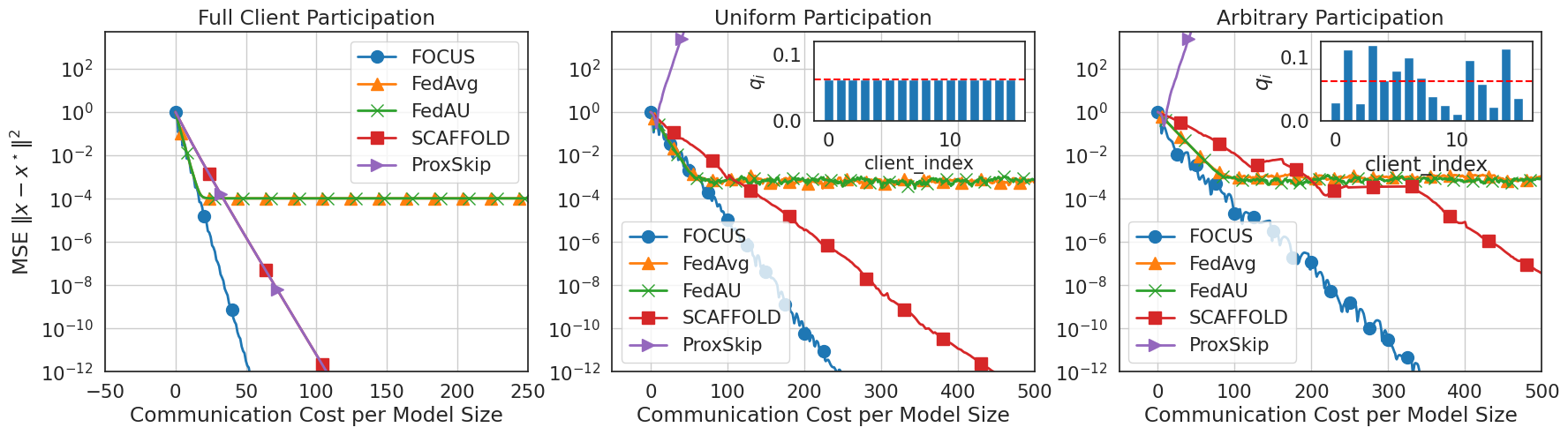
Figure 5: Convergence performance comparison of various FL algorithms. Under full client participation, FedAvg and FedAU exhibit identical performance, as do SCAFFOLD and ProxSkip, due to their theoretical equivalence in this setting. FedAvg and FedAU fail to converge to the optimal solution across all scenarios because their inherent error and bias cannot be eliminated using a fixed learning rate. ProxSkip diverges under uniform and arbitrary participation, as it is not designed for these conditions. While SCAFFOLD converges in all cases, our proposed algorithm, FOCUS , demonstrates faster convergence, especially under arbitrary participation.

Algorithm	Exact Converg.1	Strongly-Convex Complexity2	Non-Convex Complexity	Assumptions5
				Participation	Hetero. Grad.	Extra Comment
FedAvg (Li et al., 2019a)		$O(\frac{1}{\epsilon})$	$O(\frac{1}{\epsilon^{2}})$	Uniform	Bounded	Bounded gradient assumption
LocalSGD (Koloskova et al., 2020)		$O(\frac{1}{\sqrt{\epsilon}})$	$O(\frac{1}{\epsilon^{3/2}})$	Uniform	Bounded	Doubly stochastic matrix
FedAU (Wang and Ji, 2023)		–	$O\big{(}\frac{1}{\epsilon^{2}}\big{)}$	Arbitrary	Bounded	Bounded global gradient
FedAWE (Xiang et al., 2024)		–	$O(\frac{1}{\epsilon^{2}})$	Arbitrary	Bounded	Doubly stochastic matrix
SCAFFOLD (Karimireddy et al., 2020)	${\leavevmode\hbox to8.24pt{\vbox to8.24pt{\text{[drawing]}}}}^{\color[rgb]{0,0,1}3}$	$O\big{(}\log(\frac{1}{\epsilon})\big{)}$	$O(\frac{1}{\epsilon})$	Uniform	None	Comm. $2d$ vector per round
ProxSkip/ScaffNew (Mishchenko et al., 2022)		$O\big{(}\log(\frac{1}{\epsilon})\big{)}$	–	Full	None	Comm. $2d$ vector per round
FOCUS (This paper)		$O\big{(}\log(\frac{1}{\epsilon})\big{)}$	$O\big{(}\log(\frac{1}{\epsilon})\big{)}^{\color[rgb]{0,0,1}4}$	Arbitrary	None	No need to learn partici. prob.

Table 1: Comparison of multiple algorithms. ¹ exact convergence refers to the algorithm’s ability to converge to the exact solution under arbitrary sampling, without requiring a decaying learning rate. ² Complexity refers to the number of iterations required for the algorithm to achieve an error within $\epsilon$ of the optimal solution. We have removed the impact of the stochastic gradient variance in all rates. ³ There is no convergence proof of SCAFFOLD under arbitrary client participation scenario. Empirically, we observed it may be possible. ⁴ This rate is established with PL condition. ⁵ Arbitrary participation and bounded heterogeneous gradient refer to Assumption 1 and 4.

4.2 Convergence Results

Before showing the convergence rates of our algorithm, we introduce the PL assumption for non-convex cases.

Assumption 5 (PL Condition)

The global loss function $F$ satisfies the Polyak-Lojasiewicz condition:

$$\|\nabla F(x)\|^{2}\geq 2\beta\big{(}F(x)-F^{\star}\big{)},\;\;\forall x,$$ (19)

where $\beta>0$ and $F^{\star}$ is the optimal function value.

Now, the convergence rates of FOCUS are as follows:

Theorem 2

Under arbitrary participation assumption 1 and denote $q_{\min}=\min\limits_{i}q_{i}$, and $L-$Smoothness assumption 2, we can prove that FOCUS converges at the following rates with various extra assumptions on $f_{i}$:

• $\mu-$Strongly Convex: Under assumption 3, if $\eta\leq\min\{\frac{3\mu}{27NL^{2}},\frac{1}{3L(\tau-1)},\frac{q_{\min}^{3/2}}{8L\sqrt{N}}\}$,

  $$\mathbb{E}\hskip 1.42271pt\|\bar{x}_{R\tau+1}-x^{\star}\|^{2}\leq\Psi_{R}\leq(1-\eta\mu N/2)^{R}\Psi_{0}$$ (20)

• $\beta-$PL Condition: Under assumption 5, if $\eta\leq\min\{\frac{3q_{\min}}{32N},\frac{q_{\min}}{12\beta N},\frac{q_{\min}}{16L^{2}},\frac{q_{\min}^{3/2}}{8L\sqrt{N}}\}$,

  $$F(\bar{x}_{R\tau+1})-F^{\star}\leq\Phi_{R}\leq(1-\eta\beta N)^{R}\Phi_{0}$$ (21)

• General Nonconvex: With Lipschitz condition only, if $\eta\leq\min\{\frac{1}{2L(\tau-1)},\frac{q_{\min}^{3/2}}{8L\sqrt{N}},\frac{q_{\min}}{16L\sqrt{2N}},\frac{1}{4LN}\}$,

  $$\frac{1}{R}\sum_{r=0}^{R-1}\|\nabla f(x_{r\tau+1})\|^{2}\leq\frac{8(f(x_{1})-f^{\star})}{\eta NR},$$ (22)

where the Lyapunov functions $\Psi_{r}:=\mathbb{E}\hskip 1.42271pt\|\bar{x}_{r\tau+1}-x^{\star}\|^{2}+(1-8\eta\kappa LN)\mathbb{E}\hskip 1.42271pt\|\mathds{1}\bar{x}_{(r-1)\tau+1}-{\boldsymbol{x}}_{r\tau}\|^{2}_{F}$ and $\Phi_{r}=F(\bar{x}_{r\tau+1})-F^{\star}+\left(1-4\eta L^{2}\right)\mathbb{E}\hskip 1.42271pt\|\mathds{1}\bar{x}_{r\tau+1}-{\boldsymbol{x}}_{r\tau}\|^{2}$. $\hfill\hfill\blacksquare$

See the proof of the theorem in Appendix C and the comparison of our proposed algorithm with other common FL algorithms in table 1. Note $O(1/\epsilon^{2})>O(1/\epsilon)\gg O(\log(1/\epsilon))$ in terms of communication and computation complexity. Table 1 highlights the superior performance of FOCUS , which achieves the fastest convergence rate in all scenarios without particular sampling or heterogeneous gradients assumption.

4.3 Why FOCUS Can Converge Exactly for Arbitrary Participation Probabilities?

At first glance, the ability of FOCUS to achieve exact convergence under arbitrary client sampling probabilities may appear counterintuitive. Unlike other approaches, FOCUS neither requires knowledge of the specific participation probabilities nor necessitates adaptively learning these rates. The sole prerequisite for convergence is that each client maintains a non-zero probability of participation. Plus, the push-pull algorithm was never designed to solve the arbitrary sampling problem.

From an algorithmic perspective, FOCUS closely resembles the delayed/asynchronous gradient descent algorithm even though it is derived from a decentralized algorithm to fit the federated learning scenario. To see that, leveraging the tracking property of the variable ${\boldsymbol{y}}_{k}$, we have $\mathds{1}^{\mathsf{T}}{\boldsymbol{y}}_{k}=\mathds{1}^{\mathsf{T}}\nabla{\boldsymbol{f}}({\boldsymbol{x}}_{k+1})=\sum_{i=1}^{N}\nabla f_{i}(x_{k+1,i})$. Next, note at the gradient collection step, the column stochastic matrix $C_{k}$ sets the sampled client’s $y_{k,i}=0$. By employing mathematical induction, we can further deduce that $y_{k,i}$ is zero for all unsampled clients as well. Hence, we conclude that the server’s $y_{r+1}=\sum_{i=1}^{N}\nabla f_{i}(x_{k+1,i})$. Therefore, we arrive at an insightful conclusion: FOCUS effectively transforms arbitrary participation probabilities into an arbitrary delay in gradient updates. Consequently, any client participation scheme, as long as each client participates with a non-zero probability, will still guarantee exact convergence.

4.4 Numerical Validation

To validate our claims, we conducted a numerical experiment using synthetic data. The results, presented in Figure 5, were obtained by applying the algorithms to a simple ridge regression problem with the parameters $d=100$, $N=16$, $K=100$, $\lambda=0.01$, and $\tau=5$

$$F(x)=\frac{1}{N}\sum_{i=1}^{N}\sum_{k=1}^{K}\|a_{i,k}^{\mathsf{T}}x-b_{i,k}\|^{2}+\lambda\|x\|^{2}$$

All algorithms employed the same learning rate, $\eta=2e-4$. Three distinct sampling scenarios were examined: full client participation, uniform participation, and arbitrary participation. Notably, our FOCUS exhibits linear convergence and outperforms the other algorithms in all scenarios, particularly under arbitrary participation.

4.5 Extension to Stochastic Gradients

In practical machine learning scenarios, computing full gradients is often computationally prohibitive. Therefore, stochastic gradient methods are commonly employed. Our proposed algorithm can be readily extended to incorporate stochastic gradients, resulting in the variant SG-FOCUS . However, due to space constraints, we focus on the deterministic setting in the main body of this paper. A comprehensive description of SG-FOCUS , along with its convergence analysis, is provided in Appendix D. The appendix also benchmarks SG-FOCUS ’s performance on the CIFAR-10 classification task, highlighting its faster convergence and improved accuracy over other FL algorithms. This performance trend echoes that of its deterministic counterpart.

Appendix A Conventions and Notations

Under the decentralized framework, it is common to use matrix notation. We adopt the convention that the bold symbol, such as ${\boldsymbol{x}}$, is the stacked vector and the normal symbol, such as $x$, is the vector. With slight abuse of notation, we adopt the row vector convention and denote that

$${\boldsymbol{x}}_{k}=\begin{bmatrix}{-}\;x_{k,0}{-}\\ {-}\;x_{k,1}{-}\\ \cdots\\ {-}\;x_{k,N}{-}\end{bmatrix}\!\!\in\!\mathbb{R}^{N+1\times d},\;\;\;\nabla{\boldsymbol{f}}({\boldsymbol{x}}_{k})=\begin{bmatrix}\nabla f_{0}(x_{k,0})\\ \nabla f_{1}(x_{k,1})\\ \cdots\\ \nabla f_{N}(x_{k,N})\end{bmatrix}\!\!\in\!\mathbb{R}^{N+1\times d},\;\;\nabla{\boldsymbol{f}}(\mathds{1}\bar{x}_{k})= \begin{bmatrix}\nabla f_{0}(\bar{x}_{k})\\ \nabla f_{1}(\bar{x}_{k})\\ \cdots\\ \nabla f_{N}(\bar{x}_{k})\end{bmatrix}\!\!\in\!\mathbb{R}^{N+1\times d}.$$ (23)

where $\mathds{1}$ is an all-one vector. Note that in $\nabla{\boldsymbol{f}}({\boldsymbol{x}}_{k})$, each entry uses different $f_{i}$ and $x_{k,i}$. Similar usage for ${\boldsymbol{y}}_{k}$ as well. Except for ${\boldsymbol{x}}$, ${\boldsymbol{y}}$, and $\nabla{\boldsymbol{f}}$, other vectors are standard column vectors. Unlike most matrix conventions, the index of the matrix element starts from 0 instead of 1 in this paper since we set the index 0 to represent the server. Another common identity we used in the proof is

$$N\nabla F(\bar{x})=\mathds{1}^{\mathsf{T}}\nabla{\boldsymbol{f}}(\mathds{1}\bar{x}),\;\;$$ (24)

This can be easily verified when substituting the definition of $F$. The rest usage of symbols are summarized in Table 2.

Table 2: Notations in this paper

Notation	Meaning
$i$	Index of clients
$k$	Index of iterations
$r$	Index of communication round and $r=\lfloor k/\tau\rfloor\tau$
$\tau$	The number of local update steps
$S_{r}$	Indices set of clients sampled at $r-$th round
$d$	Model parameter dimension
$u,q$	Uniform / Arbitrary weighted averaging vector
$f_{i},F$	Local and global loss function
$R,V$	Some row stochastic matrix
$C$	Some column stochastic matrix

In this paper, $\|\cdot\|$ denotes $\ell_{2}$ norm for both vector and matrix usage while $\|\cdot\|_{F}$ denotes the Frobenius norm.

Appendix B Proof of the Convergence of FedAvg

This section presents a convergence analysis of the FedAvg algorithm with an arbitrary sampling/participation scheme. We focus on the strongly-convex case with a constant step size since this setting best illustrates the impact of client drift induced by local updates and bias introduced by non-uniform sampling. The following proof draws inspiration from and synthesizes several existing works (Wang and Ji, 2022; Koloskova et al., 2020; Li et al., 2019a), adapting their insights to a decentralized framework. Leveraging this framework, we are able to present a more concise proof and provide a clearer conclusion.

B.1 Reformation and Mixing Matrices

First, we rewrite the FedAvg algorithm using the decentralized matrix notation as introduced before:

$${\boldsymbol{y}}_{k+1}= R_{k}{\boldsymbol{x}}_{k}$$ (25)

$${\boldsymbol{x}}_{k+1}= V_{k}({\boldsymbol{y}}_{k+1}-\eta D_{k}\nabla{\boldsymbol{f}}({\boldsymbol{y}}_{k+1})),$$ (26)

where both $U_{k}$ and $V_{k}$ are row-stochastic matrices, and they are some realizations of random matrices representing the arbitrary sampling and $D_{k}$ are the 0-1 diagonal matrices to control the turning on and off of clients. For $\tau$ local update, it satisfies

$$R_{k}=\left\{\begin{aligned} R(S_{r}),&\;\;{\rm if}\;k=r\tau+1\\ I,&\;\;{\rm otherwsie.}\end{aligned}\right.\;\;\;\;V_{k}=\left\{\begin{aligned} V(S_{r}),&\;\;{\rm if}\;k=r\tau\\ I,&\;\;{\rm otherwsie.}\end{aligned}\right.$$ (27)

See the definition of $R(S_{r})$ and $V(S_{r})$ in main context and example in Figure 6. A noteworthy observation from (Li et al., 2019a) is that FedAvg can be equivalently reformulated without altering the trajectory of the server’s model. This reformulation considers activating all devices, where each device pulls the model from the server and performs a local update, while maintaining the same set of contributing clients for averaging. See Figure 7 as an example. Swap the order of $x$ and $y$ update, we arrive at

$${\boldsymbol{y}}_{k+1}= {\boldsymbol{x}}_{k}-\eta\nabla{\boldsymbol{f}}({\boldsymbol{x}}_{k})$$ (28)

$${\boldsymbol{x}}_{k+1}= U_{all}V_{k}{\boldsymbol{y}}_{k+1}:=W_{k}{\boldsymbol{y}}_{k+1},$$ (29)

where $W_{k}$ is a row-stochastic matrix:

$$W_{k}=\left\{\begin{aligned} I&,\;\;\;k\neq r\tau,\;\;\;\;\;\;\;\forall r=1,2,\cdots\\ W({S_{r}})&,\;\;\;k=r\tau.\;\;\;\;\;\;\;\forall r=1,2,\cdots\end{aligned}\right.$$ (30)

To better understand the property of ${W}({S_{r}})$, we provide a few concrete examples of ${W}({S_{r}})$. Suppose there are 4 clients. Under the arbitrary participation case, each round the number of participated clients is not fixed. Maybe in one round, client 1 and 3 are sampled while in another round, clients 2, 3, and 4 are sampled. The corresponding matrices are

$${W}_{\{1,3\}}=\begin{bmatrix}0&1/2&0&1/2&0\\ 0&1/2&0&1/2&0\\ 0&1/2&0&1/2&0\\ 0&1/2&0&1/2&0\\ 0&1/2&0&1/2&0\end{bmatrix},\;\;\;{W}_{\{2,3,4\}}=\begin{bmatrix}0&0&1/3&1/3&1/3\\ 0&0&1/3&1/3&1/3\\ 0&0&1/3&1/3&1/3\\ 0&0&1/3&1/3&1/3\\ 0&0&1/3&1/3&1/3\end{bmatrix}$$ (31)

It is crucial to observe that $W_{S_{r}}$ has identical rows for any possible subset $S_{r}$. Thus, it suffices to compute the expected value of the entries in any single row.

Now, we can state the property of $W({S_{r}})$. As the consequence of arbitrary participation assumption 1 and previous single row observation, we can show that

$$\bar{W}=\mathbb{E}\hskip 1.42271pt_{S_{r}}W(S_{r})=\begin{bmatrix}{-}&q^{\mathsf{T}}&{-}\\ {-}&q^{\mathsf{T}}&{-}\\ &\cdots&\\ {-}&q^{\mathsf{T}}&{-}\end{bmatrix}=\begin{bmatrix}0&q_{1}&q_{2}&\cdots&q_{N}\\ 0&q_{1}&q_{2}&\cdots&q_{N}\\ \vdots&\vdots&\vdots&\vdots&\vdots\\ 0&q_{1}&q_{2}&\cdots&q_{N}\end{bmatrix}$$ (32)

where the values $q_{i}$ is value defined in the assumption. It follows directly that this row vector is also a left eigenvector of $\mathbb{E}\hskip 1.42271ptW_{S_{r}}$, i.e., $q^{\mathsf{T}}\mathbb{E}\hskip 1.42271ptW_{S_{r}}=q^{\mathsf{T}}$, since $\sum_{i}q_{i}=1$.

$$U_{\{1,3\}}=\begin{bmatrix}1&0&0&0&0\\ 1&0&0&0&0\\ 0&0&1&0&0\\ 1&0&0&0&0\\ 0&0&0&0&1\end{bmatrix},\;\;V_{\{1,3\}}=\begin{bmatrix}1&0&0&0&0\\ 0&1&0&0&0\\ 0&0&1&0&0\\ 0&0&0&1&0\\ 0&0&0&0&1\end{bmatrix}$$

$$U_{\{1,3\}}=\begin{bmatrix}1&0&0&0&0\\ 0&1&0&0&0\\ 0&0&1&0&0\\ 0&0&0&1&0\\ 0&0&0&0&1\end{bmatrix},\;\;V_{\{1,3\}}=\begin{bmatrix}0&\frac{1}{2}&0&\frac{1}{2}&0\\ 0&1&0&0&0\\ 0&0&1&0&0\\ 0&0&0&1&0\\ 0&0&0&0&1\end{bmatrix}$$

Figure 6: Illustration of federated learning using a graph and mixing matrix. The top row depicts the pull model step, while the bottom row shows the push model and subsequent averaging step.

$$U_{\rm all}=\begin{bmatrix}1&0&0&0&0\\ 1&0&0&0&0\\ 1&0&0&0&0\\ 1&0&0&0&0\\ 1&0&0&0&0\end{bmatrix},\;\;V_{\{1,3\}}=\begin{bmatrix}1&0&0&0&0\\ 0&1&0&0&0\\ 0&0&1&0&0\\ 0&0&0&1&0\\ 0&0&0&0&1\end{bmatrix}$$

$$U_{\rm all}=\begin{bmatrix}1&0&0&0&0\\ 0&1&0&0&0\\ 0&0&1&0&0\\ 0&0&0&1&0\\ 0&0&0&0&1\end{bmatrix},\;\;V_{\{1,3\}}=\begin{bmatrix}0&\frac{1}{2}&0&\frac{1}{2}&0\\ 0&1&0&0&0\\ 0&0&1&0&0\\ 0&0&0&1&0\\ 0&0&0&0&1\end{bmatrix}$$

Figure 7: An equivalent FedAvg algorithm as Figure 6 in terms of the server model. The difference is that all clients (virtually) pull the model and run the local update but server run the partially average.

B.2 Convergence proof

As previously discussed, we will analyze FedAvg in its decentralized form using the following simplified representation:

$${\boldsymbol{y}}_{k+1}= {\boldsymbol{x}}_{k}-\eta\nabla{\boldsymbol{f}}({\boldsymbol{x}}_{k})$$ (33)

$${\boldsymbol{x}}_{k+1}= W_{k}{\boldsymbol{y}}_{k+1}$$ (34)

To start with, we define the virtual weighted iterates $\bar{x}_{k}:=q^{\mathsf{T}}{\boldsymbol{x}}_{k}$, recalling that vector $q$ is the averaging weights introduced in Assumption 1. The crucial observation is that conditional expectation $\mathbb{E}\hskip 1.42271pt_{|{\boldsymbol{y}}_{k}}\bar{x}_{k}=q^{\mathsf{T}}\mathbb{E}\hskip 1.42271ptW_{k}{\boldsymbol{y}}_{k}=q^{\mathsf{T}}{\boldsymbol{y}}_{k}$ holds for any $k$, including both local update step and model average step. When there is no ambiguity, we will just use $\mathbb{E}\hskip 1.42271pt$ for conditional expectation instead of $\mathbb{E}\hskip 1.42271pt_{|{\boldsymbol{y}}_{k}}$. Expanding the conditional expectation of $\mathbb{E}\hskip 1.42271pt\|\bar{x}_{k+1}-x^{\star}\|^{2}$, we have

$$\mathbb{E}\hskip 1.42271pt\|\bar{x}_{k+1}-x^{\star}\|^{2}= \mathbb{E}\hskip 1.42271pt\|\bar{x}_{k+1}-\mathbb{E}\hskip 1.42271pt\bar{x}_{k+1}+\mathbb{E}\hskip 1.42271pt\bar{x}_{k+1}-x^{\star}\|^{2}$$

$$= \mathbb{E}\hskip 1.42271pt\|\bar{x}_{k+1}-\mathbb{E}\hskip 1.42271pt\bar{x}_{k+1}\|^{2}+\|\mathbb{E}\hskip 1.42271pt\bar{x}_{k+1}-x^{\star}\|^{2}$$

$$= \left\{\begin{aligned} &\left\|\bar{x}_{k}-\eta q^{\mathsf{T}}\nabla{\boldsymbol{f}}({\boldsymbol{x}}_{k})-x^{\star}\right\|^{2},&k\neq r\tau\\ &\mathbb{E}\hskip 1.42271pt\left\|\bar{x}_{k+1}-q^{\mathsf{T}}{\boldsymbol{y}}_{k+1}\right\|^{2}+\left\|\bar{x}_{k}-\eta q^{\mathsf{T}}\nabla{\boldsymbol{f}}({\boldsymbol{x}}_{k})-x^{\star}\right\|^{2},&k=r\tau\end{aligned}\right.$$ (35)

where the first equality is because the cross term is zero and the second equality holds because $\mathbb{E}\hskip 1.42271pt\|\bar{x}_{k+1}-q^{\mathsf{T}}{\boldsymbol{y}}_{k+1}\|=0$ during the local update iterations ($k\neq r\tau$).

The subsequent proof follows a standard framework for analyzing decentralized algorithms. It initially establishes a descent lemma, demonstrating that the virtual weighted iterates $\bar{x}_{k}$ progressively approach a neighborhood of the optimal solution in each iteration. Subsequently, a consensus lemma is established, showing that the individual client iterates, $x_{k,i}$, gradually converge towards this weighted iterate $\bar{x}_{k}$. Finally, by combining these two lemmas, we will derive the overall convergence theorem.

B.2.1 Descent lemma

Lemma 1 (Descent Lemma of FedAvg)

Under the assumption 1, 2, and 3, the following inequality holds when the learning rate satisfies $\eta\leq\frac{1}{3L}$:

$$\left\|\bar{x}_{k}-\eta q^{\mathsf{T}}\nabla{\boldsymbol{f}}({\boldsymbol{x}}_{k})-x^{\star}\right\|^{2}\leq (1-\frac{\eta\mu}{2})\|\bar{x}_{k}-x^{\star}\|^{2}+\frac{5\eta L^{2}}{\mu}\sum_{i=1}^{N}q_{i}\|\bar{x}_{k}-x_{k,i}\|^{2}+\frac{5\eta}{\mu}\delta_{q}^{2},$$ (36)

Proof of Lemma 1:

To bound the common descent term $\|\bar{x}_{k}-\eta q^{\mathsf{T}}\nabla{\boldsymbol{f}}({\boldsymbol{x}}_{k})-x^{\star}\|^{2}$, we have

$$\left\|\bar{x}_{k}-\eta q^{\mathsf{T}}\nabla{\boldsymbol{f}}({\boldsymbol{x}}_{k})-x^{\star}\right\|^{2}$$

$$= \|\bar{x}_{k}-x^{\star}\|^{2}+\eta^{2}\|q^{\mathsf{T}}\nabla{\boldsymbol{f}}({\boldsymbol{x}}_{k})\|^{2}-2\eta\langle\bar{x}_{k}-x^{\star},q^{\mathsf{T}}\nabla{\boldsymbol{f}}({\boldsymbol{x}}_{k})\rangle$$

$$\leq \|\bar{x}_{k}-x^{\star}\|^{2}+3\eta^{2}\Big{\|}q^{\mathsf{T}}\nabla{\boldsymbol{f}}({\boldsymbol{x}}_{k})-q^{\mathsf{T}}\nabla{\boldsymbol{f}}(\mathds{1}\bar{x}_{k}))\Big{\|}^{2}+3\eta^{2}\Big{\|}q^{\mathsf{T}}\nabla{\boldsymbol{f}}(\mathds{1}\bar{x}_{k})-u^{\mathsf{T}}\nabla{\boldsymbol{f}}(\mathds{1}\bar{x}_{k}))\Big{\|}^{2}+3\eta^{2}\|\nabla F(\bar{x}_{k})\|^{2}$$

$$\;\;\;-2\eta\langle\bar{x}_{k}-x^{\star},q^{\mathsf{T}}\nabla{\boldsymbol{f}}({\boldsymbol{x}}_{k})\rangle$$

$$\leq \|\bar{x}_{k}-x^{\star}\|^{2}+3\eta^{2}L^{2}\sum_{i=1}^{N}q_{i}\|x_{k,i}-\bar{x}_{k}\|^{2}+3\eta^{2}\delta_{q}^{2}+6\eta^{2}L\big{(}F(\bar{x}_{k})-F(x^{\star})\big{)}$$

$$\;\;-2\eta\langle\bar{x}_{k}-x^{\star},q^{\mathsf{T}}\nabla{\boldsymbol{f}}({\boldsymbol{x}}_{k})\rangle,$$ (37)

where the first inequality results from Jensen’s inequality, and the second inequality utilizes (12) and the consequence of $L-$ Lipschitz smooth condition with a convex function, we have $F(x)-F(x^{\star})\geq\frac{1}{2L}\|\nabla F(x)\|^{2},\forall x$.

Next, an upper bound for the cross term can be given by

$$-2\eta\langle\bar{x}_{k}-x^{\star},q^{\mathsf{T}}\nabla{\boldsymbol{f}}({\boldsymbol{x}}_{k})\rangle$$

$$= -2\eta\langle\bar{x}_{k}-x^{\star},u^{\mathsf{T}}\nabla{\boldsymbol{f}}(\bar{{\boldsymbol{x}}}_{k})\rangle+2\eta\langle\bar{x}_{k}-x^{\star},u^{\mathsf{T}}\nabla{\boldsymbol{f}}(\bar{{\boldsymbol{x}}}_{k})-q^{\mathsf{T}}\nabla{\boldsymbol{f}}({\boldsymbol{x}}_{k})\rangle$$

$$\leq -2\eta(F(\bar{x}_{k})-F(x^{\star})+\frac{\mu}{2}\|\bar{x}_{k}-x^{\star}\|^{2})+\frac{\eta\mu}{2}\|\bar{x}_{k}-x^{\star}\|^{2}+\frac{2\eta}{\mu}\|u^{\mathsf{T}}\nabla{\boldsymbol{f}}(\bar{{\boldsymbol{x}}}_{k})-q^{\mathsf{T}}\nabla{\boldsymbol{f}}({\boldsymbol{x}}_{k})\|^{2}$$

$$\leq -\frac{\eta\mu}{2}\|\bar{x}_{k}-x^{\star}\|^{2}-2\eta\big{(}F(\bar{x}_{k})-F(x^{\star})\big{)}+\frac{4\eta}{\mu}\|q^{\mathsf{T}}\nabla{\boldsymbol{f}}(\bar{{\boldsymbol{x}}}_{k})-q^{\mathsf{T}}\nabla{\boldsymbol{f}}({\boldsymbol{x}}_{k})\|^{2}$$

$$\;\;+\frac{4\eta}{\mu}\|u^{\mathsf{T}}\nabla{\boldsymbol{f}}(\bar{{\boldsymbol{x}}}_{k})-q^{\mathsf{T}}\nabla{\boldsymbol{f}}(\bar{{\boldsymbol{x}}}_{k})\|^{2}$$

$$\leq -\frac{\eta\mu}{2}\|\bar{x}_{k}-x^{\star}\|^{2}-2\eta\big{(}F(\bar{x}_{k})-F(x^{\star})\big{)}+\frac{4\eta L^{2}}{\mu}\sum_{i=1}^{N}q_{i}\|x_{k,i}-\bar{x}_{k}\|^{2}+\frac{4\eta}{\mu}\delta_{q}^{2},$$ (38)

where the first inequality is obtained from Young’s inequality $2\langle a,b\rangle\leq\epsilon\|a\|^{2}+\frac{1}{\epsilon}\|b\|^{2}$ with $\epsilon=\mu/2$, the second inequality is due to Jensen’s inequality, and the third inequality is obtained by (12).

Combining (37) and (38), we have

$$\left\|\bar{x}_{k}-\eta q^{\mathsf{T}}\nabla{\boldsymbol{f}}({\boldsymbol{x}}_{k})-x^{\star}\right\|^{2}$$

$$\leq (1-\frac{\eta\mu}{2})\|\bar{x}_{k}-x^{\star}\|^{2}+\eta\left(\frac{4L^{2}}{\mu}+3\eta L^{2}\right)\sum_{i=1}^{N}q_{i}\|\bar{x}_{k}-x_{k,i}\|^{2}+\left(\frac{4\eta}{\mu}+3\eta^{2}\right)\delta_{q}^{2}$$

$$\;\;+(6\eta^{2}L-2\eta)\big{(}F(\bar{x}_{k})-F(x^{\star})\big{)}$$ (39)

Letting $\eta\leq\min(\frac{1}{3L},\frac{1}{3\mu})=\frac{1}{3L}$, we further have

$$\left\|\bar{x}_{k}-\eta q^{\mathsf{T}}\nabla{\boldsymbol{f}}({\boldsymbol{x}}_{k})-x^{\star}\right\|^{2}\leq (1-\frac{\eta\mu}{2})\|\bar{x}_{k}-x^{\star}\|^{2}+\frac{5\eta L^{2}}{\mu}\sum_{i=1}^{N}q_{i}\|\bar{x}_{k}-x_{k,i}\|^{2}+\frac{5\eta}{\mu}\delta_{q}^{2},$$ (40)

where we discarded the $(6\eta^{2}L-2\eta)\big{(}F(\bar{x}_{k})-F(x^{\star})\big{)}$ term since it is always negative. $\hfill\hfill\blacksquare$

B.2.2 Consensus lemma

Lemma 2 (Consensus Error of FedAvg)

Under the assumption 1, 2, and 4, the following two (weighted) consensus errors hold for any iteration $k$ when the learning rate satisfies $\eta\leq\frac{1}{4(\tau-1)L}$:

$$\sum_{i=1}^{N}q_{i}\|\bar{x}_{k}-x_{k,i}\|^{2}\leq 8\eta^{2}(\tau-1)^{2}(\delta_{q}^{2}+\sigma_{G}^{2}),\;\;\forall k$$ (41)

$$\sum_{i=1}^{N}q_{i}\|\bar{y}_{k}-y_{k,i}\|^{2}\leq 8\eta^{2}\tau^{2}(\delta_{q}^{2}+\sigma_{G}^{2}),\;\;\forall k$$ (42)

Proof of Lemma 2:

To evaluate the consensus error, the key observation is at the model average iteration, i.e., $k=r\tau$ that all clients’ model parameters $x_{k,i}$ are the same. Hence, we can express the consensus error by referring back to that point:

$$\sum_{i=1}^{N}q_{i}\|\bar{x}_{k}-x_{k,i}\|^{2}= \sum_{i=1}^{N}q_{i}\left\|x_{k_{0}}-\eta\sum_{k^{\prime}=k_{0}}^{k-1}q^{\mathsf{T}}\nabla{\boldsymbol{f}}({\boldsymbol{x}}_{k^{\prime}})-x_{k_{0}}+\eta\sum_{k^{\prime}=k_{0}}^{k-1}\nabla f_{i}(x_{k^{\prime},i})\right\|^{2}$$

$$\leq \eta^{2}(\tau-1)\sum_{i=1}^{N}\sum_{k^{\prime}=k_{0}}^{k-1}q_{i}\left\|q^{\mathsf{T}}\nabla{\boldsymbol{f}}({\boldsymbol{x}}_{k^{\prime}})-\nabla f_{i}(x_{k^{\prime},i})\right\|^{2},$$ (43)

where $k_{0}$ is the iteration that model averaging is performed, which can be calculated via $k_{0}=\tau\lfloor\frac{k}{\tau}\rfloor$. The above inequality utilizes Jensen’s inequality and observation that $k-k_{0}\leq\tau-1$. Then, we have

$$\left\|q^{\mathsf{T}}\nabla{\boldsymbol{f}}({\boldsymbol{x}}_{k^{\prime}})-\nabla f_{i}(x_{k^{\prime},i})\right\|^{2} \leq 4\left\|q^{\mathsf{T}}\nabla{\boldsymbol{f}}({\boldsymbol{x}}_{k^{\prime}})-q^{\mathsf{T}}\nabla{\boldsymbol{f}}(\mathds{1}\bar{x}_{k^{\prime}})\right\|^{2}+4\left\|q^{\mathsf{T}}\nabla{\boldsymbol{f}}(\mathds{1}\bar{x}_{k^{\prime}})-u^{\mathsf{T}}\nabla{\boldsymbol{f}}(\mathds{1}\bar{x}_{k^{\prime}})\right\|^{2}$$

$$\;\;\;\;\;+4\left\|u^{\mathsf{T}}\nabla{\boldsymbol{f}}(\mathds{1}\bar{x}_{k^{\prime}})-u^{\mathsf{T}}\nabla{\boldsymbol{f}}(\mathds{1}x_{k^{\prime},i})\right\|^{2}+4\left\|u^{\mathsf{T}}\nabla{\boldsymbol{f}}(\mathds{1}x_{k^{\prime},i})-\nabla f_{i}(\mathds{1}x_{k^{\prime},i})\right\|^{2}$$

$$\leq 4\sum_{i^{\prime}=1}^{N}q_{i^{\prime}}\|\nabla f_{i^{\prime}}(x_{k^{\prime},i^{\prime}})-\nabla f_{i}(\bar{x}_{k^{\prime}})\|^{2}+4L^{2}\|\bar{x}_{k^{\prime}}-x_{k^{\prime},i}\|^{2}+4\delta_{q}^{2}+4\sigma_{G}^{2}$$

$$\leq 4L^{2}\sum_{i^{\prime}=1}^{N}q_{i^{\prime}}\|x_{k^{\prime},i^{\prime}}-\bar{x}_{k^{\prime}}\|^{2}+4L^{2}\|\bar{x}_{k^{\prime}}-x_{k^{\prime},i}\|^{2}+4\delta_{q}^{2}+4\sigma_{G}^{2}$$ (44)

where we plus and minus $q^{\mathsf{T}}\nabla{\boldsymbol{f}}(\mathds{1}\bar{x}_{k^{\prime}})$, $u^{\mathsf{T}}\nabla{\boldsymbol{f}}(\mathds{1}\bar{x}_{k^{\prime}})$ and $u^{\mathsf{T}}\nabla{\boldsymbol{f}}(\mathds{1}x_{k^{\prime},i})$ then apply Jensen’s inequality.

Plugging (44) back to (43), we have

$$\sum_{i=1}^{N}q_{i}\|\bar{x}_{k}-x_{k,i}\|^{2}\leq \eta^{2}(\tau-1)\sum_{k^{\prime}=k_{0}}^{k-1}\left(8L^{2}\sum_{i=1}^{N}q_{i}\|x_{k^{\prime},i}-\bar{x}_{k^{\prime}}\|^{2}+4\delta_{q}^{2}+4\sigma_{G}^{2}\right)$$ (45)

Finally, we can establish a uniform bound for the consensus error using mathematical induction. Initially, note that $\sum_{i=1}^{N}q_{i}\|\bar{x}_{k_{0}}-x_{k_{0},i}\|^{2}=0$. Now, assume that $\sum_{i=1}^{N}q_{i}\|\bar{x}_{k}-x_{k,i}\|^{2}\leq\Delta$ for any $k\leq k_{0}+\tau-1$, then

$$\sum_{i=1}^{N}q_{i}\|\bar{x}_{k+\tau}-x_{k_{0}+\tau,i}\|^{2}\leq 4\eta^{2}(\tau-1)^{2}(2L^{2}\Delta+\delta_{q}^{2}+\sigma_{G}^{2})=\Delta$$ (46)

It holds when $\Delta=\frac{4\eta^{2}(K-1)^{2}(\delta_{q}^{2}+\sigma_{G}^{2})}{1-8\eta^{2}(K-1)^{2}L^{2}}$. If $\eta\leq\frac{1}{4(\tau-1)L}$, then $\Delta\leq 8\eta^{2}(\tau-1)^{2}(\delta_{q}^{2}+\sigma_{G}^{2})$. Hence, the uniform upper bound of consensus error is

$$\sum_{i=1}^{N}q_{i}\|\bar{x}_{k}-x_{k,i}\|^{2}\leq 8\eta^{2}(\tau-1)^{2}(\delta_{q}^{2}+\sigma_{G}^{2})$$ (47)

This upper bound holds for $\bar{y}_{k}$ and $y_{k,i}$ similarly with only one difference that ${\boldsymbol{y}}_{k}$ has one more inner iteration before applying the $W_{k}$ compared to ${\boldsymbol{x}}_{k}$.

$$\sum_{i=1}^{N}q_{i}\|\bar{y}_{k}-y_{k,i}\|^{2}\leq 8\eta^{2}\tau^{2}(\delta_{q}^{2}+\sigma_{G}^{2})$$ (48)

$\hfill\hfill\blacksquare$

B.2.3 Proof of Convergence Theorem 1

Proof:

Combining the above two lemmas, we conclude that for $k\neq r\tau$

$$\mathbb{E}\hskip 1.42271pt\|\bar{x}_{k+1}-x^{\star}\|^{2}\leq(1-\eta\mu/2)\|\bar{x}_{k}-x^{\star}\|^{2}+\frac{40\eta^{3}L^{2}(\tau-1)^{2}}{\mu}(\delta_{q}^{2}+\sigma_{G}^{2})+\frac{5\eta}{\mu}\delta_{q}^{2}$$ (49)

To establish the case $k=r\tau$, we need to consider the variance after the local update is done. Through previous established the consensus lemma, it is easy to verify that

$$\mathbb{E}\hskip 1.42271pt\left\|\bar{x}_{k+1}-q^{\mathsf{T}}{\boldsymbol{y}}_{k+1}\right\|^{2}= \mathbb{E}\hskip 1.42271pt\left\|q^{\mathsf{T}}W_{s_{n}}{\boldsymbol{y}}_{k+1}-q^{\mathsf{T}}{\boldsymbol{y}}_{k+1}\right\|^{2}$$

$$= \mathbb{E}\hskip 1.42271pt\left\|W_{s_{n}}[0,:]{\boldsymbol{y}}_{k+1}-q^{\mathsf{T}}{\boldsymbol{y}}_{k+1}\right\|^{2}$$

$$\leq \sum_{i=1}^{N}q_{i}\left\|y_{k+1,i}-q^{\mathsf{T}}{\boldsymbol{y}}_{k+1}\right\|^{2}$$

$$\leq 8\eta^{2}\tau^{2}(\delta_{q}^{2}+\sigma_{G}^{2}),$$

where the first equality holds because any row in the $W_{S_{n}}$ is the same, the first inequality applies Jensen’s inequality and the last inequality utilizes the consensus lemma. Substituting back to (35), we have for $k\neq r\tau$

$$\mathbb{E}\hskip 1.42271pt\|\bar{x}_{k+1}-x^{\star}\|^{2}\leq(1-\eta\mu/2)\|\bar{x}_{k}-x^{\star}\|^{2}+\frac{40\eta^{3}L^{2}(\tau-1)^{2}}{\mu}(\delta_{q}^{2}+\sigma_{G}^{2})+\frac{5\eta}{\mu}\delta_{q}^{2}+8\eta^{2}K^{2}(\delta_{q}^{2}+\sigma_{G}^{2})$$ (50)

We can simplify above two recursion as

$$A_{k+1}\leq (1-\alpha)A_{k}+B, k\neq r\tau$$ (51)

$$A_{k+1}\leq (1-\alpha)A_{k}+B+C, k=r\tau$$ (52)

where $A_{k}=\mathbb{E}\hskip 1.42271pt\|\bar{x}_{k}-x^{\star}\|^{2}$, $B=\frac{40\eta^{3}L^{2}(\tau-1)^{2}}{\mu}(\delta_{q}^{2}+\sigma_{G}^{2})+\frac{5\eta}{\mu}\delta_{q}^{2}$, and $C=8\eta^{2}K^{2}(\delta_{q}^{2}+\sigma_{G}^{2})$. Making it a $K$-step recursion together, we have

$$A_{K}\leq(1-\alpha)^{K}A_{0}+\sum_{k^{\prime}=0}^{K}(1-\alpha)^{k^{\prime}}B+\sum_{k^{\prime}=0}^{\lfloor K/\tau\rfloor}(1-\alpha)^{k^{\prime}}C$$ (53)

Letting $K\to\infty$ and substituting back, we conclude

$$\limsup_{K\to\infty}\mathbb{E}\hskip 1.42271pt\|\bar{x}_{K}-x^{\star}\|^{2}\leq\underbrace{80\eta^{2}\kappa^{2}L^{2}(\tau-1)^{2}(\delta_{q}^{2}+\sigma_{G}^{2})}_{\mbox{client drift by local update}}+\underbrace{10\kappa\delta_{q}^{2}}_{\mbox{biased sampling}}+\underbrace{16\eta\tau^{2}/\mu(\delta_{q}^{2}+\sigma_{G}^{2})}_{\mbox{data heterogeneity}},$$ (54)

where we introduce the conditional number $\kappa=L/\mu$. $\hfill\hfill\blacksquare$

As we discussed in the main context, these three terms have their own meanings. We can easily establish the following corollaries. Note$\delta_{q}^{2}=0$ under the uniform sampling case. We have

Corollary 1 (FedAvg Under the Uniform Sampling)

Under the same conditions and assumptions as theorem 1, the convergence of FedAvg with uniform sampling satisfies

$$\limsup_{K\to\infty}\mathbb{E}\hskip 1.42271pt\|\bar{x}_{K}-x^{\star}\|^{2}\leq 80\eta^{2}\kappa^{2}L^{2}(\tau-1)^{2}\sigma_{G}^{2}+16\eta\tau^{2}/\mu\sigma_{G}^{2}$$ (55)

Corollary 2 (FedAvg Under the Uniform Sampling and Single Local Update)

Under the same conditions and assumptions as theorem 1, the convergence of FedAvg with uniform sampling and $\tau=1$ satisfies

$$\limsup_{K\to\infty}\mathbb{E}\hskip 1.42271pt\|\bar{x}_{K}-x^{\star}\|^{2}\leq 16\eta\tau^{2}/\mu\sigma_{G}^{2}$$ (56)

Lastly, if the function is homogeneous among $f_{i}$, it implies $\sigma_{G}^{2}=0$. Further notice $\delta_{q}^{2}\leq\sigma_{G}^{2}=0$.

Corollary 3 (FedAvg with Homogeneous Functions)

Under the same conditions of theorem 1, FedAvg can converge exactly when $f_{i}$ is homogeneous

$$\lim_{K\to\infty}\mathbb{E}\hskip 1.42271pt\|\bar{x}_{K}-x^{\star}\|^{2}=0$$ (57)

Notably, Corollary 3 holds without requiring the assumptions of $\tau=1$ or uniform sampling. This is intuitive because arbitrary sampling becomes irrelevant in the case of homogeneous functions.

Appendix C Proof of the Convergence of FOCUS

C.1 Reformulate the Recursion

Similar to the proof of FedAvg under arbitrary client participation, we first rewrite the recursion of FOCUS so that it is easier to show the proof. Recall that the original recursion is

$${\boldsymbol{x}}_{k+1}= R_{k}({\boldsymbol{x}}_{k}-\eta D_{k}{\boldsymbol{y}}_{k})$$ (58)

$${\boldsymbol{y}}_{k+1}= C_{k}\big{(}{\boldsymbol{y}}_{k}+\nabla{\boldsymbol{f}}({\boldsymbol{x}}_{k+1})-\nabla{\boldsymbol{f}}({\boldsymbol{x}}_{k})\big{)}$$ (59)

This form is not easy to analyze when noticing the following pattern on the mixing matrix choices:

Iteration $k$:	0	1	2	$\cdots$	$\tau$	$\tau+1$	$\cdots$	$r\tau-1$	$r\tau$	$r\tau+1$	$\cdots$
$R_{k}$	Init.	$R(S_{1})$	$I$	$\cdots$	$I$	$R(S_{2})$	$\cdots$	$I$	$R(S_{r})$	$I$	$\cdots$
$C_{k}$	Init.	$I$	$I$	$\cdots$	$C(S_{1})$	$I$	$\cdots$	$C(S_{r-1})$	$I$	$I$	$\cdots$

$R(S_{r})$ and $C(S_{r})$ are not applied at the same iteration. Even worse, $R(S_{r})$ and $C(S_{r})$ are random variables and depend on each other. To avoid these difficulties, we switch the order of $x-$ and $y-$update and get the following equivalent form:

$${\boldsymbol{y}}_{k+1}= C_{k}\big{(}{\boldsymbol{y}}_{k}+\nabla{\boldsymbol{f}}({\boldsymbol{x}}_{k})-\nabla{\boldsymbol{f}}({\boldsymbol{x}}_{k-1})\big{)}$$ (60)

$${\boldsymbol{x}}_{k+1}= R_{k}({\boldsymbol{x}}_{k}-\eta D_{k}{\boldsymbol{y}}_{k+1})$$ (61)

Notice the subscript’s modification. The initial condition becomes ${\boldsymbol{y}}_{0}=\nabla{\boldsymbol{f}}({\boldsymbol{x}}_{-1})$ and ${\boldsymbol{x}}_{-1}={\boldsymbol{x}}_{0}$, which can be any values. Now, the matrices follow this new pattern

Iteration $k$:

-1

0

1

2

$\cdots$

$\tau$

$\tau+1$

$\cdots$

$r\tau-1$

$r\tau$

$r\tau+1$

$\cdots$

$C_{k}$

-

Init.

$I$

$I$

$\cdots$

$C(S_{1})$

$I$

$\cdots$

$I$

$C(S_{r-1})$

$I$

$\cdots$

$R_{k}$

Init.

$R(S_{1})$

$I$

$I$

$\cdots$

$R(S_{2})$

$I$

$\cdots$

$I$

$R(S_{r})$

$I$

$\cdots$

With this shift, both the row stochastic matrix ($R$) and column stochastic matrix ($C$) operations are applied within the same iteration. However, it is crucial to note that these operations do not correspond to the same indices of sampled clients, i.e. $S_{r}$ versus $S_{r-1}$. To further simplify the analysis, we can leverage a technique similar to the one used in the FedAvg proof: considering the collecting full set of client $y$ rather than just a subset. This is valid because the $y_{k,i}$ of non-participated clients are effectively zero. Consequently, we no longer need to take care about the correlation between R and C, significantly simplifying the analysis.

$${\boldsymbol{y}}_{k+1}= C_{k,\rm{all}}\big{(}{\boldsymbol{y}}_{k}+\nabla{\boldsymbol{f}}({\boldsymbol{x}}_{k})-\nabla{\boldsymbol{f}}({\boldsymbol{x}}_{k-1})\big{)}$$ (62)

$${\boldsymbol{x}}_{k+1}= R_{k}({\boldsymbol{x}}_{k}-\eta D_{k}{\boldsymbol{y}}_{k+1}),$$ (63)

where the definition of $C_{k,\rm{all}}$ are

$$C_{k,\rm{all}}=\begin{cases}I&\mbox{if $k\neq r\tau$}\\[8.53581pt] \begin{bmatrix}1&1&\cdots&1\\ 0&0&\cdots&0\\ &&\cdots&\\ 0&0&\cdots&0\\ \end{bmatrix}&\mbox{if $k=r\tau$}\end{cases}$$ (64)

The rest of proof will use this new form (62) - (63).

C.2 Useful Observations

Before we proceed with the proof, there are a few critical observations.

Introducing a server index selecting vector $u_{R}=[1,0,0,\cdots,0]$, it is straightforward to verify that it is the left-eigenvector of $R_{k}$ for all $k$:

$$u_{R}^{\mathsf{T}}R_{k}=u_{R}^{\mathsf{T}},\;\;\forall k.$$ (65)

Now we denote the $\bar{x}_{k}=u_{R}^{\mathsf{T}}{\boldsymbol{x}}_{k}$ and $\bar{y}_{k}=u_{R}^{\mathsf{T}}{\boldsymbol{y}}_{k}$, which can be interpreted as the server’s model parameters and gradient tracker. Utilizing the eigenvector properties and definition of $R_{k}$ and $D_{k}$, we obtain

$$\bar{x}_{k+1}=\begin{cases}\bar{x}_{k}&\;\;k\neq r\tau\\ \bar{x}_{k}-\eta\bar{y}_{k+1}&\;\;k=r\tau\\ \end{cases},\;\;\;\;\;\bar{y}_{k+1}=\begin{cases}\bar{y}_{k}&\;\;k\neq r\tau\\ \mathds{1}^{\mathsf{T}}\nabla{\boldsymbol{f}}({\boldsymbol{x}}_{k})&\;\;k=r\tau\\ \end{cases}$$ (66)

where $\bar{y}_{r\tau+1}=\mathds{1}^{\mathsf{T}}\nabla{\boldsymbol{f}}({\boldsymbol{x}}_{r\tau})$ is due to the tracking property that

$$\mathds{1}^{\mathsf{T}}{\boldsymbol{y}}_{k+1} =\mathds{1}^{\mathsf{T}}C_{k}\big{(}{\boldsymbol{y}}_{k}+\nabla{\boldsymbol{f}}({\boldsymbol{x}}_{k})-\nabla{\boldsymbol{f}}({\boldsymbol{x}}_{k-1})\big{)}=\cdots=\mathds{1}^{\mathsf{T}}\nabla{\boldsymbol{f}}({\boldsymbol{x}}_{k}),$$ (67)

and the client’s $y_{r\tau+1,i}=0$ for any clients.

The main difficulty of the analysis lies in the iteration $r\tau$ to $r\tau+1$, i.e., the gradient collecting and model pulling step. Given the information before step $r\tau$, it can be easily verified that

$$\mathbb{E}\hskip 1.42271pt\|{\boldsymbol{x}}_{r\tau+1}-{\boldsymbol{x}}_{r\tau}\|^{2}_{F}= \sum_{i=1}^{N}q_{i}\|\bar{x}_{r\tau+1}-x_{r\tau,i}\|^{2}:=\|\mathds{1}\bar{x}_{r\tau+1}-{\boldsymbol{x}}_{r\tau}\|_{Q}^{2}$$ (68)

$$\mathbb{E}\hskip 1.42271pt\|\mathds{1}\bar{x}_{r\tau+1}-{\boldsymbol{x}}_{r\tau+1}\|^{2}_{F}= \sum_{i=1}^{N}(1-q_{i})\|\bar{x}_{r\tau+1}-x_{r\tau,i}\|^{2}:=\|\mathds{1}\bar{x}_{r\tau+1}-{\boldsymbol{x}}_{r\tau}\|_{I-Q}^{2},$$ (69)

where the first equation means the difference between the model before pulling and the server’s model, and the second equation means the difference between the clients’ models after pulling and the server’s model. The last observation is the difference between model update

$$x_{(r+1)\tau,i}-x_{r\tau+1,i}= \begin{cases}0&\mbox{if \ }i\notin S_{r}\\[5.69054pt] \displaystyle\sum_{k=r\tau+2}^{(r+1)\tau}y_{k,i}&\mbox{if \ }i\in S_{r}\end{cases},$$ (70)

$$y_{r\tau+k^{\prime}+1,i}= \begin{cases}0&\mbox{if \ }i\notin S_{r}\\ \nabla f_{i}(x_{r\tau+k^{\prime},i})-\nabla f_{i}(x_{r\tau,i})&\mbox{if \ }i\in S_{r}\end{cases},\;\;$$ (71)

Using the client-only notation: $\hat{{\boldsymbol{x}}}_{k}:=[x_{k,1};x_{k,2};\cdots;x_{k,N}]\in\mathbb{R}^{N\times d}$, we have the compact form

$$\hat{{\boldsymbol{x}}}_{(r+1)\tau}-\hat{{\boldsymbol{x}}}_{r\tau+1}= D_{r}\sum_{k=r\tau+2}^{(r+1)\tau}\hat{{\boldsymbol{y}}}_{k}$$ (72)

$$\hat{{\boldsymbol{y}}}_{r\tau+k^{\prime}+1}= D_{r}\Big{(}\nabla{\boldsymbol{f}}(\hat{{\boldsymbol{x}}}_{r\tau+k^{\prime}})-\nabla{\boldsymbol{f}}(\hat{{\boldsymbol{x}}}_{r\tau})\Big{)}$$ (73)

C.3 Descent Lemma for FOCUS

Lemma 3 (Descent Lemma for FOCUS )

Under assumptions 1 (arbitrary client participation), 2 ($L$-smooth) and 3 ($\mu$-strongly convex), if the learning rate $\eta\leq\frac{1}{3L(\tau-1)}$, the expectation of server’s error can be bounded as

$$\mathbb{E}\hskip 1.42271pt\left\|\bar{x}_{(r+1)\tau+1}-x^{\star}\right\|^{2}\leq \left(1-\frac{1}{2}\eta\mu N\right)\mathbb{E}\hskip 1.42271pt\|\bar{x}_{r\tau+1}-x^{\star}\|^{2}-2\eta N(1-2\eta NL)\big{(}F(\bar{x}_{r\tau+1})-F(x^{\star})\big{)}$$

$$\;\;\;\;{}+\frac{8\eta L^{2}N}{\mu}\mathbb{E}\hskip 1.42271pt\|\mathds{1}\bar{x}_{r\tau+1}-{\boldsymbol{x}}_{r\tau}\|^{2}_{F},$$ (74)

where $x^{\star}$ is the optimal point.

Note that this lemma can only be used for the strongly-convex case, which is the most complicated case. Non-convex proof is simpler than the strongly convex one, and a similar idea can be applied there, so we make this lemma outstanding here.

Proof of Lemma 3:

The server’s error recursion from the ($r+1$)-th round to the $r$-th round is

$$\mathbb{E}\hskip 1.42271pt\left\|\bar{x}_{(r+1)\tau+1}-x^{\star}\right\|^{2}$$

$$= \mathbb{E}\hskip 1.42271pt\left\|\bar{x}_{r\tau+1}-x^{\star}-\eta\mathds{1}^{\mathsf{T}}\nabla{\boldsymbol{f}}({\boldsymbol{x}}_{(r+1)\tau})\right\|^{2}$$

$$= \|\bar{x}_{r\tau+1}-x^{\star}\|^{2}-2\eta\mathbb{E}\hskip 1.42271pt\big{\langle}\bar{x}_{r\tau+1}-x^{\star},\mathds{1}^{\mathsf{T}}\nabla{\boldsymbol{f}}({\boldsymbol{x}}_{(r+1)\tau})\big{\rangle}+\eta^{2}\mathbb{E}\hskip 1.42271pt\left\|\mathds{1}^{\mathsf{T}}\nabla{\boldsymbol{f}}({\boldsymbol{x}}_{(r+1)\tau})\right\|^{2}$$

$$\leq \|\bar{x}_{r\tau+1}-x^{\star}\|^{2}-2\eta\mathbb{E}\hskip 1.42271pt\big{\langle}\bar{x}_{r\tau+1}-x^{\star},\mathds{1}^{\mathsf{T}}\nabla{\boldsymbol{f}}({\boldsymbol{x}}_{(r+1)\tau})\big{\rangle}+2\eta^{2}\mathbb{E}\hskip 1.42271pt\left\|\mathds{1}^{\mathsf{T}}\nabla{\boldsymbol{f}}({\boldsymbol{x}}_{(r+1)\tau})-\mathds{1}^{\mathsf{T}}\nabla{\boldsymbol{f}}(\mathds{1}\bar{x}_{r\tau+1})\right\|^{2}$$

$$\;\;+2\eta^{2}N^{2}\|\nabla F(\bar{x}_{r\tau+1})\|^{2}$$

$$\leq \|\bar{x}_{r\tau+1}-x^{\star}\|^{2}-2\eta\mathbb{E}\hskip 1.42271pt\big{\langle}\bar{x}_{r\tau+1}-x^{\star},\mathds{1}^{\mathsf{T}}\nabla{\boldsymbol{f}}({\boldsymbol{x}}_{(r+1)\tau})\big{\rangle}+2\eta^{2}\mathbb{E}\hskip 1.42271pt\left\|\mathds{1}^{\mathsf{T}}\nabla{\boldsymbol{f}}({\boldsymbol{x}}_{(r+1)\tau})-\mathds{1}^{\mathsf{T}}\nabla{\boldsymbol{f}}(\mathds{1}\bar{x}_{r\tau+1})\right\|^{2}$$

$$\;\;+4\eta^{2}N^{2}L\big{(}F(\bar{x}_{r\tau+1})-F(x^{\star})\big{)},$$ (75)

where the first inequality is obtained by Jensen’s inequality and the second inequality utilizes the Lipschitz condition with convexity $\frac{1}{2L}\|\nabla F(x)\|^{2}\leq F(x)-F(x^{\star})$. The cross term can be bounded as

$$-2\eta\mathbb{E}\hskip 1.42271pt\big{\langle}\bar{x}_{r\tau+1}-x^{\star},\mathds{1}^{\mathsf{T}}\nabla{\boldsymbol{f}}({\boldsymbol{x}}_{(r+1)\tau})\big{\rangle}$$

$$= -2\eta\big{\langle}\bar{x}_{r\tau+1}-x^{\star},N\nabla F(\bar{x}_{r\tau+1})\big{\rangle}-2\eta\mathbb{E}\hskip 1.42271pt\big{\langle}\bar{x}_{r\tau+1}-x^{\star},\mathds{1}^{\mathsf{T}}\nabla{\boldsymbol{f}}({\boldsymbol{x}}_{(r+1)\tau})-\mathds{1}^{\mathsf{T}}\nabla{\boldsymbol{f}}(\mathds{1}\bar{x}_{r\tau+1})\big{\rangle}$$

$$\leq -2\eta N(F(\bar{x}_{r\tau+1})-F(x^{\star})+\frac{\mu}{2}\|\bar{x}_{r\tau+1}-x^{\star}\|^{2})+\eta\epsilon\|\bar{x}_{r\tau+1}-x^{\star}\|^{2}$$ (76)

$$\;\;\;+\frac{\eta}{\epsilon}\mathbb{E}\hskip 1.42271pt\left\|\mathds{1}^{\mathsf{T}}\nabla{\boldsymbol{f}}({\boldsymbol{x}}_{(r+1)\tau})-\mathds{1}^{\mathsf{T}}\nabla{\boldsymbol{f}}(\mathds{1}\bar{x}_{r\tau+1})\right\|^{2}$$

$$\leq -2\eta N(F(\bar{x}_{r\tau+1})-F(x^{\star}))-\frac{\eta\mu N}{2}\|\bar{x}_{r\tau+1}-x^{\star}\|^{2}+\frac{2\eta}{\mu}\mathbb{E}\hskip 1.42271pt\left\|\mathds{1}^{\mathsf{T}}\nabla{\boldsymbol{f}}({\boldsymbol{x}}_{(r+1)\tau})-\mathds{1}^{\mathsf{T}}\nabla{\boldsymbol{f}}(\mathds{1}\bar{x}_{r\tau+1})\right\|^{2},$$ (77)

where the first inequality utilizes Young’s inequality with $\epsilon$, and we set $\epsilon=\mu/2$ in the second inequality.

Plugging (77) into (75), we have

$$\mathbb{E}\hskip 1.42271pt\left\|\bar{x}_{(r+1)\tau+1}-x^{\star}\right\|^{2}\leq \left(1-\frac{\eta\mu N}{2}\right)\|\bar{x}_{r\tau+1}-x^{\star}\|^{2}-2\eta N(1-2\eta NL)\big{(}F(\bar{x}_{r\tau+1})-F(x^{\star})\big{)}$$

$$\;\;\;+2\eta\left(\frac{1}{\mu}+\eta\right)\mathbb{E}\hskip 1.42271pt\left\|\mathds{1}^{\mathsf{T}}\nabla{\boldsymbol{f}}({\boldsymbol{x}}_{(r+1)\tau})-\mathds{1}^{\mathsf{T}}\nabla{\boldsymbol{f}}(\mathds{1}\bar{x}_{r\tau+1})\right\|^{2}$$ (78)

Next, we focus on this gradient difference term:

$$\mathbb{E}\hskip 1.42271pt\left\|\mathds{1}^{\mathsf{T}}\nabla{\boldsymbol{f}}(\mathds{1}\bar{x}_{r\tau+1})-\mathds{1}^{\mathsf{T}}\nabla{\boldsymbol{f}}({\boldsymbol{x}}_{(r+1)\tau})\right\|^{2}$$ (79)

$$\leq L^{2}N\mathbb{E}\hskip 1.42271pt\|\mathds{1}\bar{x}_{r\tau+1}-{\boldsymbol{x}}_{(r+1)\tau}\|^{2}_{F}$$

$$= L^{2}N\left\|\mathds{1}\bar{x}_{r\tau+1}-{\boldsymbol{x}}_{r\tau+1}+\eta\sum_{k=r\tau+2}^{(r+1)\tau}D_{k}{\boldsymbol{y}}_{k}\right\|^{2}_{F}$$

$$\leq 2L^{2}N\|\mathds{1}\bar{x}_{r\tau+1}-{\boldsymbol{x}}_{r\tau+1}\|^{2}+2L^{2}N\left\|\eta\sum_{k=r\tau+2}^{(r+1)\tau}D_{k}{\boldsymbol{y}}_{k}\right\|^{2}_{F}$$

$$\leq 2L^{2}N\|\mathds{1}\bar{x}_{r\tau+1}-{\boldsymbol{x}}_{r\tau+1}\|^{2}+2(\tau-1)\eta^{2}L^{2}N\sum_{k=r\tau+2}^{(r+1)\tau}\left\|D_{k}{\boldsymbol{y}}_{k}\right\|^{2}_{F},$$ (80)

where the above two inequalities use Jensen’s inequality $\|\sum_{i=1}^{N}a_{i}\|^{2}\leq N\sum_{i=1}^{N}\|a_{i}\|^{2}$.

Lastly, we need to bound $y_{k,i}$ by using $L-$Lipschitz assumption and Jensen’s inequality. We just need to focus on the index $i$ that is the index among the sampled clients otherwise $y_{k,i}=0,\;\;\forall i\notin S_{r}$.

$$\|y_{k,i}\|^{2}= \|\nabla f_{i}(x_{k-1,i})-\nabla f_{i}(x_{r\tau,i})\|^{2}$$

$$\leq 2\|\nabla f_{i}(x_{k-1,i})-\nabla f_{i}(x_{r\tau+1,i})\|^{2}+2\|\nabla f_{i}(x_{r\tau+1,i})-\nabla f_{i}(x_{r\tau,i})\|^{2}$$

$$\leq 2L^{2}\|x_{k-1,i}-x_{r\tau+1,i}\|^{2}+2L^{2}\|x_{r\tau+1,i}-x_{r\tau,i}\|^{2}$$

$$\leq 2\eta^{2}L^{2}(k-r\tau-2)\sum_{k^{\prime}=r\tau+2}^{k}\|y_{k^{\prime},i}\|^{2}+2L^{2}\|x_{r\tau+1,i}-x_{r\tau,i}\|^{2}$$

$$\leq 2\eta^{2}L^{2}(\tau-1)\sum_{k^{\prime}=r\tau+2}^{(r+1)\tau}\|y_{k^{\prime},i}\|^{2}+2L^{2}\|x_{r\tau+1,i}-x_{r\tau,i}\|^{2},$$ (81)

where, in the last inequality, we just expand the non-negative term to the maximum difference cases. Hence, taking another summation of $k$ from $r\tau+2$ to $(r+1)\tau$, we obtain

$$\Big{(}1-2\eta^{2}L^{2}(\tau-1)\Big{)}\sum_{k=r\tau+2}^{(r+1)\tau}\|y_{k,i}\|^{2}\leq 2(\tau-1)L^{2}\|x_{r\tau+1,i}-x_{r\tau,i}\|^{2}$$ (82)

When $\eta\leq\frac{1}{2L\sqrt{\tau-1}}$, we conclude

$$\sum_{k=r\tau+2}^{(r+1)\tau}\|y_{k,i}\|^{2}\leq 4(\tau-1)L^{2}\|x_{r\tau+1,i}-x_{r\tau,i}\|^{2}=4(\tau-1)L^{2}\|\bar{x}_{r\tau+1}-x_{r\tau,i}\|^{2}$$ (83)

Plugging (83) back to (80), we obtain

$$\mathbb{E}\hskip 1.42271pt\left\|\mathds{1}^{\mathsf{T}}\nabla{\boldsymbol{f}}(\mathds{1}\bar{x}_{r\tau+1})-\mathds{1}^{\mathsf{T}}\nabla{\boldsymbol{f}}({\boldsymbol{x}}_{(r+1)\tau})\right\|^{2}\leq 2L^{2}N\|\mathds{1}\bar{x}_{r\tau+1}-{\boldsymbol{x}}_{r\tau}\|^{2}_{(I-Q)}$$

$$\;\;\;+8\eta^{2}(\tau-1)^{2}L^{4}N\|\mathds{1}\bar{x}_{r\tau+1}-{\boldsymbol{x}}_{r\tau}\|^{2}_{Q},$$ (84)

where the first equation means the difference between the model before pulling and the server’s model, and the second equation means the difference between the clients’ models after pulling and the server’s model. The weighted $Q$ and $I-Q$ (ref. (68)-(69)) are strictly smaller than 1, which can make the convergence proof tighter. But for simplicity, we just loosen it to 1 and got

$$\mathbb{E}\hskip 1.42271pt\left\|\mathds{1}^{\mathsf{T}}\nabla{\boldsymbol{f}}(\mathds{1}\bar{x}_{r\tau+1})-\mathds{1}^{\mathsf{T}}\nabla{\boldsymbol{f}}({\boldsymbol{x}}_{(r+1)\tau})\right\|^{2}\leq 2L^{2}N\|\mathds{1}\bar{x}_{r\tau+1}-{\boldsymbol{x}}_{r\tau}\|^{2}+8\eta^{2}(\tau-1)^{2}L^{4}N\|\mathds{1}\bar{x}_{r\tau+1}-{\boldsymbol{x}}_{r\tau}\|^{2}$$

$$\leq 3L^{2}N\|\mathds{1}\bar{x}_{r\tau+1}-{\boldsymbol{x}}_{r\tau}\|^{2}$$ (85)

where the last inequality holds when $\eta\leq\frac{1}{3(\tau-1)L}$. $\hfill\hfill\blacksquare$

C.4 Consensus Lemma for FOCUS

Lemma 4 (Consensus Lemma for FOCUS )

For Algorithm 1, under assumptions 1 and 2, if the learning rate $\eta\leq\min\left\{\frac{q_{\min}^{3/2}}{8L\sqrt{N}},\frac{q_{\min}^{3/2}}{8L(\tau-1)}\right\}$, the difference between the server’s global model and the client’s local model can be bounded as

$$\mathbb{E}\hskip 1.42271pt\|\mathds{1}\bar{x}_{r\tau+1}-{\boldsymbol{x}}_{r\tau}\|^{2}_{F}\leq\left(1-\frac{q_{\min}}{3}\right)\left\|\mathds{1}\bar{x}_{(r-1)\tau+1}-{\boldsymbol{x}}_{(r-1)\tau}\right\|^{2}_{F}+\frac{16\eta^{2}N^{2}}{3q_{\min}}\left\|\nabla F(\bar{x}_{r\tau+1})\right\|^{2}$$ (86)

Note that this consensus lemma is not related to any convex or strongly convex properties, so it can also be applied in nonconvex cases.

Proof of Lemma 4:

Here, we focus on how different the server’s model at the $r$-round and the client’s model just before pulling the model from the server. Taking the conditional expectation, we have

$$\mathbb{E}\hskip 1.42271pt\|\mathds{1}\bar{x}_{r\tau+1}-{\boldsymbol{x}}_{r\tau}\|^{2}_{F}= \mathbb{E}\hskip 1.42271pt\left\|\mathds{1}\bar{x}_{(r-1)\tau+1}-\eta\mathds{1}\bar{y}_{r\tau+1}-{\boldsymbol{x}}_{(r-1)\tau+1}+\eta\sum_{k=(r-1)\tau+2}^{r\tau}D_{k}{\boldsymbol{y}}_{k}\right\|^{2}_{F}$$

$$\leq \frac{1}{\rho}\mathbb{E}\hskip 1.42271pt\left\|\mathds{1}\bar{x}_{(r-1)\tau+1}-{\boldsymbol{x}}_{(r-1)\tau+1}\right\|^{2}_{F}+\frac{2\eta^{2}}{1-\rho}\mathbb{E}\hskip 1.42271pt\|\mathds{1}\bar{y}_{r\tau+1}\|^{2}+\frac{2\eta^{2}}{1-\rho}\mathbb{E}\hskip 1.42271pt\left\|\sum_{k=(r-1)\tau+2}^{r\tau}D_{k}{\boldsymbol{y}}_{k}\right\|^{2},$$ (87)

where the inequality above uses Jensen’s inequality $\|a+b\|^{2}\leq\frac{1}{\rho}\|a\|^{2}+\frac{1}{1-\rho}\|b\|^{2}$ and $\rho$ here can be any value between 0 and 1 (exclusively). For each term, we know

$$\mathbb{E}\hskip 1.42271pt\left\|\mathds{1}\bar{x}_{(r-1)\tau+1}-{\boldsymbol{x}}_{(r-1)\tau+1}\right\|^{2}_{F}= \sum_{i=1}^{N}(1-q_{i})\|\bar{x}_{(r-1)\tau+1}-x_{(r-1)\tau,i}\|^{2}$$

$$\leq (1-q_{\min})\left\|\mathds{1}\bar{x}_{(r-1)\tau+1}-{\boldsymbol{x}}_{(r-1)\tau}\right\|^{2}_{F}$$ (88)

and

$$\|\mathds{1}\bar{y}_{r\tau+1}\|^{2}\leq 2\left\|\mathds{1}^{\mathsf{T}}\nabla{\boldsymbol{f}}({\boldsymbol{x}}_{r\tau})-\mathds{1}^{\mathsf{T}}\nabla{\boldsymbol{f}}(\mathds{1}\bar{x}_{r\tau+1})\right\|^{2}+2\left\|N\nabla F(\bar{x}_{r\tau+1})\right\|^{2}$$

$$\leq 2NL^{2}\|\mathds{1}\bar{x}_{r\tau+1}-{\boldsymbol{x}}_{r\tau}\|^{2}_{F}+2\left\|N\nabla F(\bar{x}_{r\tau+1})\right\|^{2}$$ (89)

and

$$\mathbb{E}\hskip 1.42271pt\left\|\sum_{k=(r-1)\tau+2}^{r\tau}D_{k}{\boldsymbol{y}}_{k}\right\|^{2}\leq (\tau-1)\mathbb{E}\hskip 1.42271pt\sum_{k=r\tau+2}^{(r+1)\tau}\|D_{k}{\boldsymbol{y}}_{k}\|^{2}$$

$$\leq 4(\tau-1)^{2}L^{2}\sum_{i=1}^{N}q_{i}\|\bar{x}_{r\tau+1}-x_{r\tau,i}\|^{2}$$

$$\leq 4(\tau-1)^{2}L^{2}\|\mathds{1}\bar{x}_{r\tau+1}-{\boldsymbol{x}}_{r\tau}\|^{2}$$ (90)

Putting (C.4) (89), (90) back to (87) and selecting $\rho=\frac{1-q_{\min}}{1-q_{\min}/2}=1-\frac{q_{\min}}{2-q_{\min}}$, we obtain

$$\mathbb{E}\hskip 1.42271pt\|\mathds{1}\bar{x}_{r\tau+1}-{\boldsymbol{x}}_{r\tau}\|^{2}_{F}\leq \left(1-\frac{q_{\min}}{2}\right)\|\mathds{1}\bar{x}_{(r-1)\tau+1}-{\boldsymbol{x}}_{(r-1)\tau}\|^{2}_{F}+\frac{4\eta^{2}NL^{2}(2-q_{\min})}{q_{\min}}\|\mathds{1}\bar{x}_{r\tau+1}-{\boldsymbol{x}}_{r\tau}\|^{2}_{F}$$

$$\;\;\;{}+\frac{4\eta^{2}N^{2}(2-q_{\min})}{q_{\min}}\left\|\nabla F(\bar{x}_{r\tau+1})\right\|^{2}+\frac{8\eta^{2}(\tau-1)^{2}L^{2}(2-q_{\min})}{q_{\min}}\|\mathds{1}\bar{x}_{r\tau+1}-{\boldsymbol{x}}_{r\tau}\|^{2}$$

$$\leq \left(1-\frac{q_{\min}}{2}\right)\|\mathds{1}\bar{x}_{(r-1)\tau+1}-{\boldsymbol{x}}_{(r-1)\tau}\|^{2}_{F}+\frac{8\eta^{2}NL^{2}}{q_{\min}}\|\mathds{1}\bar{x}_{r\tau+1}-{\boldsymbol{x}}_{r\tau}\|^{2}_{F}$$

$$\;\;\;{}+\frac{8\eta^{2}N^{2}}{q_{\min}}\left\|\nabla F(\bar{x}_{r\tau+1})\right\|^{2}+\frac{16\eta^{2}(\tau-1)^{2}L^{2}}{q_{\min}}\|\mathds{1}\bar{x}_{r\tau+1}-{\boldsymbol{x}}_{r\tau}\|^{2}$$ (91)

If $\eta\leq\min\left\{\frac{q_{\min}^{3/2}}{8L\sqrt{N}},\frac{q_{\min}^{3/2}}{8L(\tau-1)}\right\}$, we have

$$\left(1-\frac{q^{2}_{\min}}{4}\right)\mathbb{E}\hskip 1.42271pt\|\mathds{1}\bar{x}_{r\tau+1}-{\boldsymbol{x}}_{r\tau}\|^{2}_{F}\leq \left(1-\frac{q_{\min}}{2}\right)\left\|\mathds{1}\bar{x}_{(r-1)\tau+1}-{\boldsymbol{x}}_{(r-1)\tau}\right\|^{2}_{F}+\frac{8\eta^{2}N^{2}}{q_{\min}}\left\|\nabla F(\bar{x}_{r\tau+1})\right\|^{2}$$ (92)

Simplifying it further, we obtain

$$\mathbb{E}\hskip 1.42271pt\|\mathds{1}\bar{x}_{r\tau+1}-{\boldsymbol{x}}_{r\tau}\|^{2}_{F}\leq\left(1-\frac{q_{\min}}{3}\right)\left\|\mathds{1}\bar{x}_{(r-1)\tau+1}-{\boldsymbol{x}}_{(r-1)\tau}\right\|^{2}_{F}+\frac{16\eta^{2}N^{2}}{3q_{\min}}\left\|\nabla F(\bar{x}_{r\tau+1})\right\|^{2}$$ (93)

$\hfill\hfill\blacksquare$

C.5 Proof of the Convergence of FOCUS ($\mu-$Strong Convexity)

Proof of Theorem 2 ($\mu-$Strongly Convex Case):

By Lemmas 3 and 4, we have two recursions

$$\mathbb{E}\hskip 1.42271pt\left\|\bar{x}_{(r+1)\tau+1}-x^{\star}\right\|^{2}\leq \left(1-\frac{\eta\mu N}{2}\right)\mathbb{E}\hskip 1.42271pt\|\bar{x}_{r\tau+1}-x^{\star}\|^{2}-2\eta N(1-2\eta NL)\big{(}F(\bar{x}_{r\tau+1})-F(x^{\star})\big{)}$$

$$\;\;\;\;{}+\frac{8\eta L^{2}N}{\mu}\mathbb{E}\hskip 1.42271pt\|\mathds{1}\bar{x}_{r\tau+1}-{\boldsymbol{x}}_{r\tau}\|^{2}$$ (94)

$$\mathbb{E}\hskip 1.42271pt\|\mathds{1}\bar{x}_{r\tau+1}-{\boldsymbol{x}}_{r\tau}\|^{2}_{F}\leq \left(1-\frac{q_{\min}}{3}\right)\left\|\mathds{1}\bar{x}_{(r-1)\tau+1}-{\boldsymbol{x}}_{(r-1)\tau}\right\|^{2}_{F}+\frac{16\eta^{2}N^{2}}{3q_{\min}}\left\|\nabla F(\bar{x}_{r\tau+1})\right\|^{2}$$ (95)

$$\leq \left(1-\frac{q_{\min}}{3}\right)\left\|\mathds{1}\bar{x}_{(r-1)\tau+1}-{\boldsymbol{x}}_{(r-1)\tau}\right\|^{2}_{F}+\frac{32\eta^{2}N^{2}L}{3q_{\min}}\big{(}F(\bar{x}_{r\tau+1})-F(x^{\star})\big{)}$$ (96)

To lighten the notation, we let $A_{r+1}=\mathbb{E}\hskip 1.42271pt\|\bar{x}_{(r+1)\tau+1}-x^{\star}\|^{2}$ and $B_{r}=\mathbb{E}\hskip 1.42271pt\|\mathds{1}\bar{x}_{r\tau+1}-{\boldsymbol{x}}_{r\tau}\|^{2}_{F}$. Therefore, we have

$$A_{r+1}\leq \left(1-\frac{\eta\mu N}{2}\right)A_{r}-2\eta N(1-2\eta NL)\big{(}F(\bar{x}_{r\tau+1})-F(x^{\star})\big{)}+\frac{8\eta L^{2}N}{\mu}B_{r}$$ (97)

$$B_{r}\leq \left(1-\frac{q_{\min}}{3}\right)B_{r-1}+\frac{32\eta^{2}N^{2}L}{3q_{\min}}\big{(}F(\bar{x}_{r\tau+1})-F(x^{\star})\big{)}$$ (98)

After summing up them, the term about $\big{(}F(\bar{x}_{r\tau+1})-F(x^{\star})\big{)}$ is negative, so we directly remove it in the upper bound. Then, we get

$$A_{r+1}+\left(1-\frac{8\eta L^{2}N}{\mu}\right)B_{r}\leq \left(1-\frac{\eta\mu N}{2}\right)A_{r}+\left(1-\frac{q_{\min}}{3}\right)B_{r-1}$$

$$\leq \left(1-\frac{\eta\mu N}{2}\right)\left(A_{r}+\big{(}1-\frac{8\eta L^{2}N}{\mu}\big{)}B_{r-1}\right),$$ (99)

where (99) holds when $\eta\leq\frac{2q_{\min}}{3N\left(\frac{8L^{2}}{\mu}+\frac{\mu}{2}\right)}$. $\hfill\hfill\blacksquare$

Hence, we conclude that FOCUS achieves the linear convergence rate of $(1-\eta\mu N/2)$ under the strongly-convex condition.

C.6 Proof of the Convergence of FOCUS (Non-Convexity with PL Assumption)

Proof of Theorem 2 (Nonconvex Case with PL Assumption):

Using the $L-$Lipschitz condition, we have

$$F(\bar{x}_{(r+1)\tau+1})$$

$$\leq F(\bar{x}_{(r+1)\tau})-\eta\langle\nabla F(\bar{x}_{(r+1)\tau}),\mathds{1}^{\mathsf{T}}\nabla{\boldsymbol{f}}({\boldsymbol{x}}_{(r+1)\tau})\rangle+\frac{\eta^{2}L}{2}\left\|\mathds{1}^{\mathsf{T}}\nabla{\boldsymbol{f}}({\boldsymbol{x}}_{(r+1)\tau})\right\|^{2}$$

$$= F(\bar{x}_{r\tau+1})-\eta\langle\nabla F(\bar{x}_{r\tau+1}),\mathds{1}^{\mathsf{T}}\nabla{\boldsymbol{f}}({\boldsymbol{x}}_{(r+1)\tau})\rangle+\frac{\eta^{2}L}{2}\left\|\mathds{1}^{\mathsf{T}}\nabla{\boldsymbol{f}}({\boldsymbol{x}}_{(r+1)\tau})\right\|^{2}$$

$$\leq F(\bar{x}_{r\tau+1})-\eta\langle\nabla F(\bar{x}_{r\tau+1}),\mathds{1}^{\mathsf{T}}\nabla{\boldsymbol{f}}({\boldsymbol{x}}_{(r+1)\tau})\rangle+\eta^{2}L\left\|N\nabla F(\bar{x}_{r\tau+1})-\mathds{1}^{\mathsf{T}}\nabla{\boldsymbol{f}}({\boldsymbol{x}}_{(r+1)\tau})\right\|^{2}$$ (100)

$$\;\;\;+\eta^{2}N^{2}L\|\nabla F(\bar{x}_{r\tau+1})\|^{2},$$ (101)

where the last inequality uses Jensen’s inequality.

Using the parallelogram identity to bound the cross term, we have

$$-\eta\langle\nabla F(\bar{x}_{r\tau+1}),\mathds{1}^{\mathsf{T}}\nabla{\boldsymbol{f}}({\boldsymbol{x}}_{(r+1)\tau})\rangle$$

$$= -\frac{\eta}{N}\langle N\nabla F(\bar{x}_{r\tau+1}),\mathds{1}^{\mathsf{T}}\nabla{\boldsymbol{f}}({\boldsymbol{x}}_{(r+1)\tau})\rangle$$

$$= \frac{\eta}{2N}\left\|\mathds{1}^{\mathsf{T}}\nabla{\boldsymbol{f}}(\mathds{1}\bar{x}_{r\tau+1})-\mathds{1}^{\mathsf{T}}\nabla{\boldsymbol{f}}({\boldsymbol{x}}_{(r+1)\tau})\right\|^{2}-\frac{\eta N}{2}\|\nabla F(\bar{x}_{r\tau+1})\|^{2}-\frac{\eta}{2N}\left\|\mathds{1}^{\mathsf{T}}\nabla{\boldsymbol{f}}({\boldsymbol{x}}_{(r+1)\tau})\right\|^{2}$$

$$\leq \frac{\eta}{2N}\left\|\mathds{1}^{\mathsf{T}}\nabla{\boldsymbol{f}}(\mathds{1}\bar{x}_{r\tau+1})-\mathds{1}^{\mathsf{T}}\nabla{\boldsymbol{f}}({\boldsymbol{x}}_{(r+1)\tau})\right\|^{2}-\frac{\eta N}{2}\|\nabla F(\bar{x}_{r\tau+1})\|^{2}$$ (102)

where we discard the non-positive term in the last step. Substituting back, we have

$$F(\bar{x}_{(r+1)\tau+1})\leq F(\bar{x}_{r\tau+1})+\left(\frac{\eta}{2N}+\eta^{2}L\right)\left\|\mathds{1}\nabla{\boldsymbol{f}}(\mathds{1}\bar{x}_{r\tau+1})-\mathds{1}^{\mathsf{T}}\nabla{\boldsymbol{f}}({\boldsymbol{x}}_{(r+1)\tau})\right\|^{2}$$

$$\;\;\;-\left(\frac{\eta N}{2}-\eta^{2}N^{2}L\right)\|\nabla F(\bar{x}_{r\tau+1})\|^{2}$$

$$\leq F(\bar{x}_{r\tau+1})+\frac{\eta}{N}\left\|\mathds{1}\nabla{\boldsymbol{f}}(\mathds{1}\bar{x}_{r\tau+1})-\mathds{1}^{\mathsf{T}}\nabla{\boldsymbol{f}}({\boldsymbol{x}}_{(r+1)\tau})\right\|^{2}-\eta N\|\nabla F(\bar{x}_{r\tau+1})\|^{2}$$

$$\leq F(\bar{x}_{r\tau+1})+\frac{\eta}{N}\left\|\mathds{1}\nabla{\boldsymbol{f}}(\mathds{1}\bar{x}_{r\tau+1})-\mathds{1}^{\mathsf{T}}\nabla{\boldsymbol{f}}({\boldsymbol{x}}_{(r+1)\tau})\right\|^{2}-\eta\beta N\left(F(\bar{x}_{r\tau+1})-F^{\star}\right)$$

$$\;\;\;-\frac{\eta N}{2}\|\nabla F(\bar{x}_{r\tau+1})\|^{2},$$ (103)

where the second inequality follows $\eta\leq\min\{\frac{1}{4LN},\frac{1}{2(\tau-1)LN}\}$ and the last inequality we split $-\eta N\|\nabla F(\bar{x}_{r\tau+1})\|^{2}$ into two parts and applying PL-condition for one part. Next, we minus $F^{\star}$ on the both sides to obtain:

$$F(\bar{x}_{(r+1)\tau+1})-F^{\star}\leq (1-\eta\beta N)\big{(}F(\bar{x}_{r\tau+1})-F^{\star}\big{)}+\frac{\eta}{N}\left\|\mathds{1}\nabla{\boldsymbol{f}}(\mathds{1}\bar{x}_{r\tau+1})-\mathds{1}^{\mathsf{T}}\nabla{\boldsymbol{f}}({\boldsymbol{x}}_{(r+1)\tau})\right\|^{2}$$

$$\;\;\;-\frac{\eta N}{2}\|\nabla F(\bar{x}_{r\tau+1})\|^{2}$$ (104)

Recalling the previous result (84):

$$\mathbb{E}\hskip 1.42271pt\left\|\mathds{1}^{\mathsf{T}}\nabla{\boldsymbol{f}}(\mathds{1}\bar{x}_{r\tau+1})-\mathds{1}^{\mathsf{T}}\nabla{\boldsymbol{f}}({\boldsymbol{x}}_{(r+1)\tau})\right\|^{2}\leq \big{(}2L^{2}N+8\eta^{2}(\tau-1)^{2}L^{4}N\big{)}\|\mathds{1}\bar{x}_{r\tau+1}-{\boldsymbol{x}}_{r\tau}\|^{2}$$ (105)

Putting (105) back to (104), we have

$$F(\bar{x}_{(r+1)\tau+1})-F^{\star}\leq (1-\eta\beta N)\big{(}F(\bar{x}_{r\tau+1})-F^{\star}\big{)}+4\eta L^{2}\|\mathds{1}\bar{x}_{r\tau+1}-{\boldsymbol{x}}_{r\tau}\|^{2}-\frac{\eta N}{2}\|\nabla F(\bar{x}_{r\tau+1})\|^{2}$$ (106)

Recalling the Lemma 4, we know

$$\mathbb{E}\hskip 1.42271pt\|\mathds{1}\bar{x}_{r\tau+1}-{\boldsymbol{x}}_{r\tau}\|^{2}_{F}\leq \left(1-\frac{q_{\min}}{3}\right)\left\|\mathds{1}\bar{x}_{(r-1)\tau+1}-{\boldsymbol{x}}_{(r-1)\tau}\right\|^{2}_{F}+\frac{16\eta^{2}N^{2}}{3q_{\min}}\left\|\nabla F(\bar{x}_{r\tau+1})\right\|^{2}$$ (107)

With a condition $\eta\leq\min\{\frac{3q_{\min}}{32N},\frac{q_{\min}}{3\beta N(4-q_{\min})},\frac{q_{\min}}{16L^{2}}\}$, we denote $A_{r}=F(\bar{x}_{r\tau+1})-F^{\star}$ and $B_{r}=\mathbb{E}\hskip 1.42271pt\|\mathds{1}\bar{x}_{r\tau+1}-{\boldsymbol{x}}_{r\tau}\|^{2}$, and then we have

$$A_{r+1}+\left(1-4\eta L^{2}\right)B_{r}\leq (1-\eta\beta N)A_{r}+\left(1-\frac{q_{\min}}{3}\right)B_{r-1}$$

$$= (1-\eta\beta N)\left(A_{r}+\frac{1-\frac{q_{\min}}{3}}{1-\eta\beta N}B_{r-1}\right)$$

$$\leq (1-\eta\beta N)\left(A_{r}+\big{(}1-\frac{q_{\min}}{4}\big{)}B_{r-1}\right)$$

$$\leq (1-\eta\beta N)\left(A_{r}+\left(1-4\eta L^{2}\right)B_{r-1}\right)$$ (108)

Therefore, we conclude that FOCUS achieves the linear convergence rate of $(1-\eta\beta N)$ in the nonconvex case with PL condition. $\hfill\hfill\blacksquare$

C.7 Proof of the Convergence of FOCUS (General Non-Convexity)

Proof of Theorem 2 (General Nonconvex Case):

We begin with $L-$Lipschitz condition:

$$F(\bar{x}_{(r+1)\tau+1})\leq F(\bar{x}_{r\tau+1})-\eta\left\langle\nabla F(\bar{x}_{r\tau+1}),\mathds{1}^{\mathsf{T}}\nabla{\boldsymbol{f}}({\boldsymbol{x}}_{(r+1)\tau})\right\rangle+\frac{\eta^{2}L}{2}\left\|\mathds{1}^{\mathsf{T}}\nabla{\boldsymbol{f}}({\boldsymbol{x}}_{(r+1)\tau})\right\|^{2}$$

$$\leq F(\bar{x}_{r\tau+1})-\eta\left\langle\nabla F(\bar{x}_{r\tau+1}),\mathds{1}^{\mathsf{T}}\nabla{\boldsymbol{f}}({\boldsymbol{x}}_{(r+1)\tau})\right\rangle$$

$$\;\;\;+\eta^{2}L\left\|N\nabla F(\bar{x}_{r\tau+1})-\mathds{1}^{\mathsf{T}}\nabla{\boldsymbol{f}}({\boldsymbol{x}}_{(r+1)\tau})\right\|^{2}+\eta^{2}N^{2}L\|\nabla F(\bar{x}_{r\tau+1})\|^{2},$$ (109)

where the last inequality utilizes the Jensen’s inequality.

Then, we deal with the cross term:

$$-\eta\left\langle\nabla F(\bar{x}_{r\tau+1}),\mathds{1}^{\mathsf{T}}\nabla{\boldsymbol{f}}({\boldsymbol{x}}_{(r+1)\tau})\right\rangle$$

$$= -\eta N\|\nabla F(\bar{x}_{r\tau+1})\|^{2}+\eta\left\langle\nabla F(\bar{x}_{r\tau+1}),N\nabla F(\bar{x}_{r\tau+1})-\mathds{1}^{\mathsf{T}}\nabla{\boldsymbol{f}}({\boldsymbol{x}}_{(r+1)\tau})\right\rangle$$

$$\leq -\frac{\eta N}{2}\|\nabla F(\bar{x}_{r\tau+1})\|^{2}+\frac{\eta}{2N}\left\|\mathds{1}\nabla{\boldsymbol{f}}(\mathds{1}\bar{x}_{r\tau+1})-\mathds{1}^{\mathsf{T}}\nabla{\boldsymbol{f}}({\boldsymbol{x}}_{(r+1)\tau})\right\|^{2}$$ (110)

Substituting (110) back to (109), we have

$$\frac{\eta N}{2}(1-2\eta NL)\mathbb{E}\hskip 1.42271pt\|\nabla F(\bar{x}_{r\tau+1})\|^{2}\leq F(\bar{x}_{r\tau+1})-\mathbb{E}\hskip 1.42271ptF(\bar{x}_{(r+1)\tau+1})$$

$$+\left(\frac{\eta}{2N}+\eta^{2}L\right)\mathbb{E}\hskip 1.42271pt\left\|\mathds{1}^{\mathsf{T}}\nabla{\boldsymbol{f}}(\bar{x}_{r\tau+1})-\mathds{1}^{\mathsf{T}}\nabla{\boldsymbol{f}}({\boldsymbol{x}}_{(r+1)\tau})\right\|^{2}$$ (111)

To bound the term $\left\|\mathds{1}^{\mathsf{T}}\nabla{\boldsymbol{f}}(\bar{x}_{r\tau+1})-\mathds{1}^{\mathsf{T}}\nabla{\boldsymbol{f}}({\boldsymbol{x}}_{(r+1)\tau})\right\|^{2}$, we can directly use the result (84), so we will obtain:

$$\frac{\eta N}{2}(1-2\eta NL)\mathbb{E}\hskip 1.42271pt\|\nabla F(\bar{x}_{r\tau+1})\|^{2}\leq F(\bar{x}_{r\tau+1})-\mathbb{E}\hskip 1.42271ptF(\bar{x}_{(r+1)\tau+1})$$

$$+\left(\frac{\eta}{2N}+\eta^{2}L\right)\left(2L^{2}N+8\eta^{2}(\tau-1)^{2}L^{4}N\right)\mathbb{E}\hskip 1.42271pt\|\mathds{1}\bar{x}_{r\tau+1}-{\boldsymbol{x}}_{r\tau}\|^{2}$$ (112)

Then, when $\eta\leq\min\{\frac{1}{4LN},\frac{1}{2L(\tau-1)}\}$, we can get $1/2\leq(1-2\eta NL)$, $\eta^{2}L\leq\eta/2N$ and $8\eta^{2}(\tau-1)^{2}L^{4}N\leq 2L^{2}N$. Thus, we can simplify the coefficients further as follows:

$$\mathbb{E}\hskip 1.42271pt\|\nabla F(\bar{x}_{r\tau+1})\|^{2}\leq \frac{4}{\eta N}\Big{(}F(\bar{x}_{r\tau+1})-F(\bar{x}_{(r+1)\tau+1})\Big{)}+\frac{16L^{2}}{N}\mathbb{E}\hskip 1.42271pt\left\|\mathds{1}\bar{x}_{r\tau+1}-{\boldsymbol{x}}_{r\tau}\right\|^{2}$$ (113)

Recalling the Lemma 4, we know

$$\mathbb{E}\hskip 1.42271pt\|\mathds{1}\bar{x}_{r\tau+1}-{\boldsymbol{x}}_{r\tau}\|^{2}_{F}\leq\left(1-\frac{q_{\min}}{3}\right)\left\|\mathds{1}\bar{x}_{(r-1)\tau+1}-{\boldsymbol{x}}_{(r-1)\tau}\right\|^{2}_{F}+\frac{16\eta^{2}N^{2}}{3q_{\min}}\left\|\nabla F(\bar{x}_{r\tau+1})\right\|^{2}$$ (114)

We denote that $A_{r}=\mathbb{E}\hskip 1.42271pt\|\nabla F(\bar{x}_{r\tau+1})\|^{2}$, $B_{r}=F(\bar{x}_{r\tau+1})$ and $C_{r}=\mathbb{E}\hskip 1.42271pt\|\mathds{1}\bar{x}_{r\tau+1}-{\boldsymbol{x}}_{r\tau}\|^{2}$.

Through (114) and (113), we have the following two recursions:

$$A_{r}\leq \frac{4}{\eta N}\Big{(}B_{r}-B_{r+1}\Big{)}+\frac{16L^{2}}{N}C_{r}$$ (115)

$$C_{r}\leq \left(1-\frac{q_{\min}}{3}\right)C_{r-1}+\frac{16\eta^{2}N^{2}}{3q_{\min}}A_{r}$$ (116)

Taking the summation from $r=0$ to $R-1$, we have

$$\frac{1}{R}\sum_{r=0}^{R-1}C_{r}=\frac{1}{R}\sum_{r=1}^{R-1}C_{r}\leq \left(1-\frac{q_{\min}}{3}\right)\sum_{r=1}^{R-1}C_{r-1}+\frac{16\eta^{2}N^{2}}{3Rq_{\min}}\frac{1}{R}\sum_{r=1}^{R-1}A_{r}$$

$$\leq \left(1-\frac{q_{\min}}{3}\right)\frac{1}{R}\sum_{r=0}^{R-1}C_{r}+\frac{16\eta^{2}N^{2}}{3Rq_{\min}}\sum_{r=0}^{R-1}A_{r}$$ (117)

Note $C_{0}=0$ and we shift the subscripts in the second inequation since adding a non-negative term always holds. Therefore,

$$\frac{1}{R}\sum_{r=0}^{R-1}C_{r}\leq\frac{16\eta^{2}N^{2}}{Rq^{2}_{\min}}\sum_{r=0}^{R-1}A_{r}$$ (118)

Lastly, noting

$$\frac{1}{R}\sum_{r=0}^{R-1}A_{r}\leq\frac{4}{\eta N}(B_{0}-B_{R})+\frac{16L^{2}}{NR}\sum_{r=0}^{R-1}C_{r}$$

$$\Longrightarrow\;\;\;\;\;\; \left(1-\frac{256\eta^{2}L^{2}N}{q_{\min}^{2}}\right)\frac{1}{R}\sum_{r=0}^{R-1}A_{r}\leq\frac{4}{\eta N}(B_{0}-B_{R})$$

$$\Longrightarrow\;\;\;\;\;\; \frac{1}{R}\sum_{r=0}^{R-1}\mathbb{E}\hskip 1.42271pt\|\nabla F(\bar{x}_{r\tau+1})\|^{2}\leq\frac{8\Big{(}F(\bar{x}_{1})-F(\bar{x}^{\star})\Big{)}}{\eta NR},$$ (119)

where the last inequality follows $\eta\leq\frac{q_{\min}}{16L\sqrt{2N}}$. $\hfill\hfill\blacksquare$

Appendix D Extensions to Stochastic Gradient Case ( SG-FOCUS )

When applying the optimization algorithm to the machine learning problem, we need to use stochastic gradients instead of gradient oracle. Only one line change of FOCUS is required to support the stochastic gradient case, which is highlighted in Algorithm 2. Notably, the past stochastic gradient is $\nabla f_{i}(x_{k-1,i};\xi_{k-1})$ instead of $\nabla f_{i}(x_{k-1,i};\xi_{k})$. This choice preserves the crucial tracking property. Furthermore, this approach offers a computational advantage by allowing us to store and reuse the prior stochastic gradient, thus avoiding redundant computations.

Algorithm 2 SG-FOCUS (Stochastic Gradient Version of FOCUS)

1: Initialize: Choose learning rate $\eta$ and local update $\tau$. At server, set a random $x_{0}$, $y_{0}=0$ and set $\nabla f_{i}(x_{i,-1})=0$ at all clients.

2: for $r=0,1,...,R-1$ do

3:  Arbitrarily sample client index set $S_{r}$

4:  for $i$ in $S_{r}$ parallel do

5:   $x_{0,i}=x_{r},\;y_{0,i}=0$ $\triangleright$ Pull model $x_{r}$ from server while $y_{r}$ is NOT pulled

6:   for $k=0,\cdots,\tau-1$ do

7:    $\displaystyle y_{k+1,i}=y_{k,i}+\nabla f_{i}(x_{k,i};\xi_{k})-\nabla f_{i}(x_{k-1,i};\xi_{k-1})$ $\triangleright$ $x_{-1,i}$ is $x_{\tau,i}$ in last participation

8:    $x_{k+1,i}=x_{k,i}-\eta y_{k+1,i}$

9:   end for

10:  end for

11:  $y_{r+1}=y_{r}+\sum_{i\in S_{r}}y_{\tau,i}$ $\triangleright$ Pushing $y_{i,\tau}$ to server (Not averaging)

12:  $x_{r+1}=x_{r}-\eta y_{r+1}$ $\triangleright$ Client model $x_{i,\tau}$ is NEVER pushed.

13: end for

Before showing the lemmas and proof of SG-FOCUS , we introduce an assumption of unbiased stochastic gradients with bounded variance as follows.

Assumption 6 (Unbiased Stochastic Gradients with Bounded Variance)

The stochastic gradient computed by clients or the server is unbiased with bounded variance:

$$\mathbb{E}\hskip 1.42271pt[\nabla f_{i}(x;\xi)]=\nabla f_{i}(x)\;\;\textrm{ and }\;\;\mathbb{E}\hskip 1.42271pt\left\|\nabla f_{i}(x;\xi)-\nabla f_{i}(x)\right\|^{2}\leq\sigma^{2},$$ (120)

where $\xi$ is the data sample.

D.1 Descent Lemma for SG-FOCUS

Lemma 5

Under assumption 1, 2, 3 and 6, if $\eta\leq\min\{\frac{\mu}{128(\tau-1)^{2}L^{2}N},\frac{1}{2\sqrt{2}(\tau-1)L}\}$, the expectation of server’s error can be bounded as

$$\mathbb{E}\hskip 1.42271pt\left\|\bar{x}_{(r+1)\tau+1}-x^{\star}\right\|^{2}\leq \left(1-\frac{\eta\mu N}{2}\right)\mathbb{E}\hskip 1.42271pt\|\bar{x}_{r\tau+1}-x^{\star}\|^{2}-2\eta N(1-2\eta NL)\big{(}F(\bar{x}_{r\tau+1})-F(x^{\star})\big{)}$$

$$\;\;\;+\frac{16\eta L^{2}N}{\mu}\|\mathds{1}\bar{x}_{r\tau+1}-{\boldsymbol{x}}_{r\tau}\|^{2}+2\eta^{2}\sigma^{2},$$

where $x^{\star}$ is the optimal point. Note that this lemma can only be used for strongly convex cases.

Proof of Lemma 5:

The server’s error recursion from the ($r+1$)-th round to the $r$-th round is

$$\mathbb{E}\hskip 1.42271pt\left\|\bar{x}_{(r+1)\tau+1}-x^{\star}\right\|^{2}$$

$$= \mathbb{E}\hskip 1.42271pt\left\|\bar{x}_{r\tau+1}-x^{\star}-\eta\mathds{1}^{\mathsf{T}}\nabla{\boldsymbol{f}}({\boldsymbol{x}}_{(r+1)\tau};\xi_{(r+1)\tau})\right\|^{2}$$

$$= \|\bar{x}_{r\tau+1}-x^{\star}\|^{2}-2\eta\mathbb{E}\hskip 1.42271pt\big{\langle}\bar{x}_{r\tau+1}-x^{\star},\mathds{1}^{\mathsf{T}}\nabla{\boldsymbol{f}}({\boldsymbol{x}}_{(r+1)\tau};\xi_{(r+1)\tau})\big{\rangle}+\eta^{2}\mathbb{E}\hskip 1.42271pt\left\|\mathds{1}^{\mathsf{T}}\nabla{\boldsymbol{f}}({\boldsymbol{x}}_{(r+1)\tau};\xi_{(r+1)\tau})\right\|^{2}$$

$$\leq \|\bar{x}_{r\tau+1}-x^{\star}\|^{2}-2\eta\big{\langle}\bar{x}_{r\tau+1}-x^{\star},\mathds{1}^{\mathsf{T}}\nabla{\boldsymbol{f}}({\boldsymbol{x}}_{(r+1)\tau})\big{\rangle}+\eta^{2}\sigma^{2}$$

$$\;\;+2\eta^{2}\left\|\mathds{1}^{\mathsf{T}}\nabla{\boldsymbol{f}}({\boldsymbol{x}}_{(r+1)\tau})-\mathds{1}^{\mathsf{T}}\nabla{\boldsymbol{f}}(\mathds{1}\bar{x}_{r\tau+1})\right\|^{2}+2\eta^{2}N^{2}\|\nabla F(\bar{x}_{r\tau+1})\|^{2}$$

$$\leq \|\bar{x}_{r\tau+1}-x^{\star}\|^{2}-2\eta\big{\langle}\bar{x}_{r\tau+1}-x^{\star},\mathds{1}^{\mathsf{T}}\nabla{\boldsymbol{f}}({\boldsymbol{x}}_{(r+1)\tau})\big{\rangle}+\eta^{2}\sigma^{2}$$

$$\;\;+2\eta^{2}\left\|\mathds{1}^{\mathsf{T}}\nabla{\boldsymbol{f}}({\boldsymbol{x}}_{(r+1)\tau})-\mathds{1}^{\mathsf{T}}\nabla{\boldsymbol{f}}(\mathds{1}\bar{x}_{r\tau+1})\right\|^{2}+4\eta^{2}N^{2}L\big{(}F(\bar{x}_{r\tau+1})-F(x^{\star})\big{)},$$ (121)

where the first inequality is obtained by Jensen’s inequality and the second inequality utilizes the Lipschitz condition $\frac{1}{2L}\|\nabla F(x)\|^{2}\leq F(x)-F(x^{\star})$. The cross term can be bounded as

$$-2\eta\big{\langle}\bar{x}_{r\tau+1}-x^{\star},\mathds{1}^{\mathsf{T}}\nabla{\boldsymbol{f}}({\boldsymbol{x}}_{(r+1)\tau})\big{\rangle}$$

$$= -2\eta\big{\langle}\bar{x}_{r\tau+1}-x^{\star},N\nabla F(\bar{x}_{r\tau+1})\big{\rangle}-2\eta\big{\langle}\bar{x}_{r\tau+1}-x^{\star},\mathds{1}^{\mathsf{T}}\nabla{\boldsymbol{f}}({\boldsymbol{x}}_{(r+1)\tau})-\mathds{1}^{\mathsf{T}}\nabla{\boldsymbol{f}}(\mathds{1}\bar{x}_{r\tau+1})\big{\rangle}$$

$$\leq -2\eta N(F(\bar{x}_{r\tau+1})-F(x^{\star})+\frac{\mu}{2}\|\bar{x}_{r\tau+1}-x^{\star}\|^{2})+\eta\epsilon\|\bar{x}_{r\tau+1}-x^{\star}\|^{2}$$

$$\;\;+\frac{\eta}{\epsilon}\left\|\mathds{1}^{\mathsf{T}}\nabla{\boldsymbol{f}}({\boldsymbol{x}}_{(r+1)\tau})-\mathds{1}^{\mathsf{T}}\nabla{\boldsymbol{f}}(\mathds{1}\bar{x}_{r\tau+1})\right\|^{2}$$

$$\leq -2\eta N(F(\bar{x}_{r\tau+1})-F(x^{\star}))-\frac{\eta\mu N}{2}\|\bar{x}_{r\tau+1}-x^{\star}\|^{2}+\frac{2\eta}{\mu}\left\|\mathds{1}^{\mathsf{T}}\nabla{\boldsymbol{f}}({\boldsymbol{x}}_{(r+1)\tau})-\mathds{1}^{\mathsf{T}}\nabla{\boldsymbol{f}}(\mathds{1}\bar{x}_{r\tau+1})\right\|^{2},$$ (122)

where the first inequality utilizes Young’s inequality with $\epsilon$, and we set $\epsilon=\mu/2$ in the second inequality.

Plugging (122) into (121), we have

$$\mathbb{E}\hskip 1.42271pt\left\|\bar{x}_{(r+1)\tau+1}-x^{\star}\right\|^{2}\leq \left(1-\frac{\eta\mu N}{2}\right)\|\bar{x}_{r\tau+1}-x^{\star}\|^{2}-2\eta N(1-2\eta NL)\big{(}F(\bar{x}_{r\tau+1})-F(x^{\star})\big{)}$$

$$\;\;\;\;{}+2\eta\left(\frac{1}{\mu}+\eta\right)\left\|\mathds{1}^{\mathsf{T}}\nabla{\boldsymbol{f}}({\boldsymbol{x}}_{(r+1)\tau})-\mathds{1}^{\mathsf{T}}\nabla{\boldsymbol{f}}(\mathds{1}\bar{x}_{r\tau+1})\right\|^{2}+\eta^{2}\sigma^{2}$$ (123)

Now, we focus on this gradient difference term:

$$\mathbb{E}\hskip 1.42271pt\left\|\mathds{1}^{\mathsf{T}}\nabla{\boldsymbol{f}}(\mathds{1}\bar{x}_{r\tau+1})-\mathds{1}^{\mathsf{T}}\nabla{\boldsymbol{f}}({\boldsymbol{x}}_{(r+1)\tau})\right\|^{2}$$

$$\leq L^{2}N\mathbb{E}\hskip 1.42271pt\|\mathds{1}\bar{x}_{r\tau+1}-{\boldsymbol{x}}_{(r+1)\tau}\|^{2}_{F}$$

$$= L^{2}N\mathbb{E}\hskip 1.42271pt\left\|\mathds{1}\bar{x}_{r\tau+1}-{\boldsymbol{x}}_{r\tau+1}+\eta\sum_{k=r\tau+2}^{(r+1)\tau}D_{k}{\boldsymbol{y}}_{k}\right\|^{2}_{F}$$

$$\leq 2L^{2}N\|\mathds{1}\bar{x}_{r\tau+1}-{\boldsymbol{x}}_{r\tau+1}\|^{2}+2L^{2}N\mathbb{E}\hskip 1.42271pt\left\|\eta\sum_{k=r\tau+2}^{(r+1)\tau}D_{k}{\boldsymbol{y}}_{k}\right\|^{2}_{F}$$

$$\leq 2L^{2}N\|\mathds{1}\bar{x}_{r\tau+1}-{\boldsymbol{x}}_{r\tau+1}\|^{2}+2(\tau-1)\eta^{2}L^{2}N\mathbb{E}\hskip 1.42271pt\sum_{k=r\tau+2}^{(r+1)\tau}\left\|D_{k}{\boldsymbol{y}}_{k}\right\|^{2}_{F},$$ (124)

where the last two inequalities use the Jensen’s inequality $\|\sum_{i=1}^{N}a_{i}\|^{2}\leq N\sum_{i=1}^{N}\|a_{i}\|^{2}$.

Next, we need to bound $y_{k,i}$ by using $L-$Lipshitz assumption and Jensen’s inequality. Assume $i$ is the index among the sampled clients:

$$\mathbb{E}\hskip 1.42271pt\|y_{k,i}\|^{2}= \mathbb{E}\hskip 1.42271pt\|\nabla f_{i}(x_{k-1,i};\xi_{k-1,i})-\nabla f_{i}(x_{r\tau,i};\xi_{r\tau,i})\|^{2}$$

$$\leq 4\mathbb{E}\hskip 1.42271pt\|\nabla f_{i}(x_{k-1,i};\xi_{k-1,i})-\nabla f_{i}(x_{k-1,i})\|^{2}+4\mathbb{E}\hskip 1.42271pt\|\nabla f_{i}(x_{k-1,i})-\nabla f_{i}(x_{r\tau+1,i})\|^{2}$$

$$\;\;\;+4\mathbb{E}\hskip 1.42271pt\|\nabla f_{i}(x_{r\tau+1,i})-\nabla f_{i}(x_{r\tau,i})\|^{2}+4\mathbb{E}\hskip 1.42271pt\|\nabla f_{i}(x_{r\tau,i})-\nabla f_{i}(x_{r\tau,i};\xi_{r\tau,i})\|^{2}$$

$$\leq 4L^{2}\|x_{k-1,i}-x_{r\tau+1,i}\|^{2}+4L^{2}\|x_{r\tau+1,i}-x_{r\tau,i}\|^{2}+8\sigma^{2}$$

$$\leq 4\eta^{2}L^{2}(k-r\tau-2)\sum_{k^{\prime}=r\tau+2}^{k}\|y_{k^{\prime},i}\|^{2}+4L^{2}\|x_{r\tau+1,i}-x_{r\tau,i}\|^{2}+8\sigma^{2}$$

$$\leq 4\eta^{2}L^{2}(\tau-1)\sum_{k^{\prime}=r\tau+2}^{(r+1)\tau}\|y_{k^{\prime},i}\|^{2}+4L^{2}\|x_{r\tau+1,i}-x_{r\tau,i}\|^{2}+8\sigma^{2},$$

where, in the last inequality, we just expand the non-negative term to the maximum difference cases. Hence, taking another summation of $k$ from $r\tau+2$ to $(r+1)\tau$, we obtain

$$\Big{(}1-4\eta^{2}L^{2}(\tau-1)\Big{)}\sum_{k=r\tau+2}^{(r+1)\tau}\mathbb{E}\hskip 1.42271pt\|y_{k,i}\|^{2}\leq 4(\tau-1)L^{2}\|x_{r\tau+1,i}-x_{r\tau,i}\|^{2}+8(\tau-1)\sigma^{2}$$

When $1/2\leq\big{(}1-4\eta^{2}L^{2}(\tau-1)\big{)}$ i.e., $\eta\leq\frac{1}{2L\sqrt{2(\tau-1)}}$, we conclude

$$\mathbb{E}\hskip 1.42271pt\sum_{k=r\tau+2}^{(r+1)\tau}\|y_{k,i}\|^{2}\leq 8(\tau-1)L^{2}\|x_{r\tau+1,i}-x_{r\tau,i}\|^{2}+16(\tau-1)\sigma^{2}$$

$$= 8(\tau-1)L^{2}\|\bar{x}_{r\tau+1}-x_{r\tau,i}\|^{2}+16(\tau-1)\sigma^{2}$$ (125)

Plugging (125) back to (124), we obtain

$$\mathbb{E}\hskip 1.42271pt\left\|\mathds{1}^{\mathsf{T}}\nabla{\boldsymbol{f}}(\mathds{1}\bar{x}_{r\tau+1})-\mathds{1}^{\mathsf{T}}\nabla{\boldsymbol{f}}({\boldsymbol{x}}_{(r+1)\tau})\right\|^{2}\leq \big{(}2L^{2}N+16\eta^{2}(\tau-1)^{2}L^{4}N\big{)}\|\mathds{1}\bar{x}_{r\tau+1}-{\boldsymbol{x}}_{r\tau}\|^{2}$$

$$\;\;+32\eta^{2}(\tau-1)^{2}L^{2}N\sigma^{2},$$ (126)

Plugging (126) into (123), we obtain

$$\mathbb{E}\hskip 1.42271pt\left\|\bar{x}_{(r+1)\tau+1}-x^{\star}\right\|^{2}\leq \left(1-\frac{\eta\mu N}{2}\right)\mathbb{E}\hskip 1.42271pt\|\bar{x}_{r\tau+1}-x^{\star}\|^{2}-2\eta N(1-2\eta NL)\big{(}F(\bar{x}_{r\tau+1})-F(x^{\star})\big{)}$$

$$\;\;\;+2\eta\left(\frac{1}{\mu}+\eta\right)\left(2L^{2}N+16\eta^{2}(\tau-1)^{2}L^{4}N\right)\|\mathds{1}\bar{x}_{r\tau+1}-{\boldsymbol{x}}_{r\tau}\|^{2}$$

$$\;\;\;+\eta^{2}\sigma^{2}+2\eta\left(\frac{1}{\mu}+\eta\right)32\eta^{2}(\tau-1)^{2}L^{2}N\sigma^{2}$$

$$\leq \left(1-\frac{\eta\mu N}{2}\right)\mathbb{E}\hskip 1.42271pt\|\bar{x}_{r\tau+1}-x^{\star}\|^{2}-2\eta N(1-2\eta NL)\big{(}F(\bar{x}_{r\tau+1})-F(x^{\star})\big{)}$$

$$\;\;\;+\frac{16\eta L^{2}N}{\mu}\|\mathds{1}\bar{x}_{r\tau+1}-{\boldsymbol{x}}_{r\tau}\|^{2}+2\eta^{2}\sigma^{2},$$

where the last inequality follows $\eta\leq\min\{\frac{1}{\mu},\frac{\mu}{128(\tau-1)^{2}L^{2}N},\frac{1}{2\sqrt{2}(\tau-1)L}\}=\min\{\frac{\mu}{128(\tau-1)^{2}L^{2}N},\frac{1}{2\sqrt{2}(\tau-1)L}\}$. $\hfill\hfill\blacksquare$

D.2 Consensus Lemma for SG-FOCUS

Lemma 6 (Consensus Lemma for SG-FOCUS )

For Algorithm 2, under assumptions 1, 2 and 6, if the learning rate $\eta\leq\min\left\{\frac{q_{\min}^{3/2}}{4L\sqrt{6N}},\frac{q_{\min}^{3/2}}{8\sqrt{2}L(\tau-1)}\right\}$, the difference between the server’s global model and the client’s local model can be bounded as

$$\mathbb{E}\hskip 1.42271pt\|\mathds{1}\bar{x}_{r\tau+1}-{\boldsymbol{x}}_{r\tau}\|^{2}_{F}\leq \left(1-\frac{q_{\min}}{3}\right)\left\|\mathds{1}\bar{x}_{(r-1)\tau+1}-{\boldsymbol{x}}_{(r-1)\tau}\right\|^{2}_{F}+\frac{8\eta^{2}N^{2}}{q_{\min}}\left\|\nabla F(\bar{x}_{r\tau+1})\right\|^{2}+\frac{8\eta^{2}N}{q_{\min}}\sigma^{2}$$

Note that this consensus lemma is not related to any convex or strongly convex properties, so it can also be applied in nonconvex cases.

Proof of Lemma 6:

Here, we focus on how different the server’s model at the $r$-round and the client’s model just before pulling the model from the server. Taking the conditional expectation, we have

$$\mathbb{E}\hskip 1.42271pt\|\mathds{1}\bar{x}_{r\tau+1}-{\boldsymbol{x}}_{r\tau}\|^{2}_{F}= \mathbb{E}\hskip 1.42271pt\left\|\mathds{1}\bar{x}_{(r-1)\tau+1}-\eta\mathds{1}\bar{y}_{r\tau+1}-{\boldsymbol{x}}_{(r-1)\tau+1}+\eta\sum_{k=(r-1)\tau+2}^{r\tau}D_{k}{\boldsymbol{y}}_{k}\right\|^{2}_{F}$$

$$\leq \frac{1}{\rho}\mathbb{E}\hskip 1.42271pt\left\|\mathds{1}\bar{x}_{(r-1)\tau+1}-{\boldsymbol{x}}_{(r-1)\tau+1}\right\|^{2}_{F}+\frac{2\eta^{2}}{1-\rho}\mathbb{E}\hskip 1.42271pt\|\mathds{1}\bar{y}_{r\tau+1}\|^{2}$$

$$\;\;+\frac{2\eta^{2}}{1-\rho}\mathbb{E}\hskip 1.42271pt\left\|\sum_{k=(r-1)\tau+2}^{r\tau}D_{k}{\boldsymbol{y}}_{k}\right\|^{2},$$ (127)

where the inequality above uses Jensen’s inequality $\|a+b\|^{2}\leq\frac{1}{\rho}\|a\|^{2}+\frac{1}{1-\rho}\|b\|^{2}$ and $\rho$ here can be any value between 0 and 1 (exclusive). For each term, we know

$$\mathbb{E}\hskip 1.42271pt\left\|\mathds{1}\bar{x}_{(r-1)\tau+1}-{\boldsymbol{x}}_{(r-1)\tau+1}\right\|^{2}_{F}= \sum_{i=1}^{N}(1-q_{i})\|\bar{x}_{(r-1)\tau+1}-x_{(r-1)\tau,i}\|^{2}$$

$$\leq (1-q_{\min})\left\|\mathds{1}\bar{x}_{(r-1)\tau+1}-{\boldsymbol{x}}_{(r-1)\tau}\right\|^{2}_{F}$$ (128)

and

$$\|\bar{y}_{r\tau+1}\|^{2}\leq 3\left\|\mathds{1}^{\mathsf{T}}\nabla{\boldsymbol{f}}({\boldsymbol{x}}_{r\tau};\xi_{r\tau})-\mathds{1}^{\mathsf{T}}\nabla{\boldsymbol{f}}(\mathds{1}\bar{x}_{r\tau})\right\|^{2}+3\left\|\mathds{1}^{\mathsf{T}}\nabla{\boldsymbol{f}}(\mathds{1}\bar{x}_{r\tau})-\mathds{1}^{\mathsf{T}}\nabla{\boldsymbol{f}}(\mathds{1}\bar{x}_{r\tau+1})\right\|^{2}$$

$$\;\;+3\left\|N\nabla F(\bar{x}_{r\tau+1})\right\|^{2}$$

$$\leq 3N\sigma^{2}+3NL^{2}\|\mathds{1}\bar{x}_{r\tau+1}-{\boldsymbol{x}}_{r\tau}\|^{2}_{F}+3\left\|N\nabla F(\bar{x}_{r\tau+1})\right\|^{2}$$ (129)

and

$$\mathbb{E}\hskip 1.42271pt\left\|\sum_{k=(r-1)\tau+2}^{r\tau}D_{k}{\boldsymbol{y}}_{k}\right\|^{2}\leq (\tau-1)\mathbb{E}\hskip 1.42271pt\sum_{k=r\tau+2}^{(r+1)\tau}\|D_{k}{\boldsymbol{y}}_{k}\|^{2}$$

$$\leq 4(\tau-1)^{2}L^{2}\sum_{i=1}^{N}q_{i}\|\bar{x}_{r\tau+1}-x_{r\tau,i}\|^{2}$$

$$\leq 4(\tau-1)^{2}L^{2}\|\mathds{1}\bar{x}_{r\tau+1}-{\boldsymbol{x}}_{r\tau}\|^{2}$$ (130)

Putting (D.2), (129), (130) back to (127) and selecting $\rho=\frac{1-q_{\min}}{1-q_{\min}/2}=1-\frac{q_{\min}}{2-q_{\min}}$, we obtain

$$\mathbb{E}\hskip 1.42271pt\|\mathds{1}\bar{x}_{r\tau+1}-{\boldsymbol{x}}_{r\tau}\|^{2}_{F}\leq \left(1-\frac{q_{\min}}{2}\right)\|\mathds{1}\bar{x}_{(r-1)\tau+1}-{\boldsymbol{x}}_{(r-1)\tau}\|^{2}_{F}+\frac{6\eta^{2}NL^{2}(2-q_{\min})}{q_{\min}}\|\mathds{1}\bar{x}_{r\tau+1}-{\boldsymbol{x}}_{r\tau}\|^{2}_{F}$$

$$\;\;\;{}+\frac{6\eta^{2}N^{2}(2-q_{\min})}{q_{\min}}\left\|\nabla F(\bar{x}_{r\tau+1})\right\|^{2}+\frac{6\eta^{2}N(2-q_{\min})}{q_{\min}}\sigma^{2}$$

$$\;\;\;+\frac{8\eta^{2}(\tau-1)^{2}L^{2}(2-q_{\min})}{q_{\min}}\|\mathds{1}\bar{x}_{r\tau+1}-{\boldsymbol{x}}_{r\tau}\|^{2}$$

$$\leq \left(1-\frac{q_{\min}}{2}\right)\|\mathds{1}\bar{x}_{(r-1)\tau+1}-{\boldsymbol{x}}_{(r-1)\tau}\|^{2}_{F}+\frac{12\eta^{2}NL^{2}}{q_{\min}}\|\mathds{1}\bar{x}_{r\tau+1}-{\boldsymbol{x}}_{r\tau}\|^{2}_{F}$$

$$\;\;\;{}+\frac{12\eta^{2}N^{2}}{q_{\min}}\left\|\nabla F(\bar{x}_{r\tau+1})\right\|^{2}+\frac{12\eta^{2}NL^{2}}{q_{\min}}\sigma^{2}+\frac{16\eta^{2}(\tau-1)^{2}L^{2}}{q_{\min}}\|\mathds{1}\bar{x}_{r\tau+1}-{\boldsymbol{x}}_{r\tau}\|^{2}$$

If $\eta\leq\min\left\{\frac{q_{\min}^{3/2}}{4L\sqrt{6N}},\frac{q_{\min}^{3/2}}{8\sqrt{2}L(\tau-1)}\right\}$, we have

$$\left(1-\frac{q^{2}_{\min}}{4}\right)\mathbb{E}\hskip 1.42271pt\|\mathds{1}\bar{x}_{r\tau+1}-{\boldsymbol{x}}_{r\tau}\|^{2}_{F}\leq \left(1-\frac{q_{\min}}{2}\right)\left\|\mathds{1}\bar{x}_{(r-1)\tau+1}-{\boldsymbol{x}}_{(r-1)\tau}\right\|^{2}_{F}$$

$$\;\;+\frac{12\eta^{2}N^{2}}{q_{\min}}\left\|\nabla F(\bar{x}_{r\tau+1})\right\|^{2}+\frac{12\eta^{2}N}{q_{\min}}\sigma^{2}$$

Simplifying it further, we obtain

$$\mathbb{E}\hskip 1.42271pt\|\mathds{1}\bar{x}_{r\tau+1}-{\boldsymbol{x}}_{r\tau}\|^{2}_{F}\leq\left(1-\frac{q_{\min}}{3}\right)\left\|\mathds{1}\bar{x}_{(r-1)\tau+1}-{\boldsymbol{x}}_{(r-1)\tau}\right\|^{2}_{F}+\frac{8\eta^{2}N^{2}}{q_{\min}}\left\|\nabla F(\bar{x}_{r\tau+1})\right\|^{2}+\frac{8\eta^{2}N}{q_{\min}}\sigma^{2}$$

$\hfill\hfill\blacksquare$

D.3 Proof of the Convergence of SG-FOCUS ($\mu-$Strong Convexity)

Theorem 3 (Convergence of SG-FOCUS for Strongly Convex Functions)

Under assumption 1, 2, 3 and 6, if the learning rate $\eta\leq\min\left\{\frac{2q_{\min}}{3N\left(\frac{16L^{2}}{\mu}+\frac{\mu}{2}\right)},\frac{q_{\min}^{3/2}}{4L\sqrt{6N}},\frac{q_{\min}^{3/2}}{8\sqrt{2}L(\tau-1)},\frac{\mu}{128(\tau-1)^{2}L^{2}N}\right\}$,

$$\Gamma_{R}\leq \left(1-\frac{\eta\mu N}{2}\right)^{R}\Gamma_{0}+\frac{4(q_{\min}+N^{2})}{\mu Nq_{\min}}\eta\sigma^{2},$$

where $\Gamma_{r}:=\mathbb{E}\hskip 1.42271pt\|\bar{x}_{(r+1)\tau+1}-x^{\star}\|^{2}+\big{(}1-8\eta L^{2}N/\mu\big{)}\mathbb{E}\hskip 1.42271pt\|\mathds{1}\bar{x}_{(r-1)\tau+1}-{\boldsymbol{x}}_{(r-1)\tau}\|^{2}_{F}$.

Proof of Theorem 3:

By Lemmas 5 and 6, we have two recursions

$$\mathbb{E}\hskip 1.42271pt\left\|\bar{x}_{(r+1)\tau+1}-x^{\star}\right\|^{2}\leq \left(1-\frac{\eta\mu N}{2}\right)\mathbb{E}\hskip 1.42271pt\|\bar{x}_{r\tau+1}-x^{\star}\|^{2}-2\eta N(1-2\eta NL)\big{(}F(\bar{x}_{r\tau+1})-F(x^{\star})\big{)}$$

$$\;\;\;\;{}+\frac{16\eta L^{2}N}{\mu}\mathbb{E}\hskip 1.42271pt\|\mathds{1}\bar{x}_{r\tau+1}-{\boldsymbol{x}}_{r\tau}\|^{2}+2\eta^{2}\sigma^{2}$$

$$\mathbb{E}\hskip 1.42271pt\|\mathds{1}\bar{x}_{r\tau+1}-{\boldsymbol{x}}_{r\tau}\|^{2}_{F}\leq \left(1-\frac{q_{\min}}{3}\right)\left\|\mathds{1}\bar{x}_{(r-1)\tau+1}-{\boldsymbol{x}}_{(r-1)\tau}\right\|^{2}_{F}+\frac{8\eta^{2}N^{2}}{q_{\min}}\left\|\nabla F(\bar{x}_{r\tau+1})\right\|^{2}+\frac{8\eta^{2}N^{2}}{q_{\min}}\sigma^{2}$$

$$\leq \left(1-\frac{q_{\min}}{3}\right)\left\|\mathds{1}\bar{x}_{(r-1)\tau+1}-{\boldsymbol{x}}_{(r-1)\tau}\right\|^{2}_{F}+\frac{16\eta^{2}N^{2}L}{q_{\min}}\big{(}F(\bar{x}_{r\tau+1})-F(x^{\star})\big{)}+\frac{8\eta^{2}N^{2}}{q_{\min}}\sigma^{2}$$

To lighten the notation, we let $A_{r+1}=\mathbb{E}\hskip 1.42271pt\|\bar{x}_{(r+1)\tau+1}-x^{\star}\|^{2}$ and $B_{r}=\mathbb{E}\hskip 1.42271pt\|\mathds{1}\bar{x}_{r\tau+1}-{\boldsymbol{x}}_{r\tau}\|^{2}_{F}$. Therefore, we have

$$A_{r+1}\leq \left(1-\frac{\eta\mu N}{2}\right)A_{r}-2\eta N(1-2\eta NL)\big{(}F(\bar{x}_{r\tau+1})-F(x^{\star})\big{)}+\frac{16\eta L^{2}N}{\mu}B_{r}+2\eta^{2}\sigma^{2}$$

$$B_{r}\leq \left(1-\frac{q_{\min}}{3}\right)B_{r-1}+\frac{16\eta^{2}N^{2}L}{q_{\min}}\big{(}F(\bar{x}_{r\tau+1})-F(x^{\star})\big{)}+\frac{8\eta^{2}N^{2}}{q_{\min}}\sigma^{2}$$

After summing up them, the term about $\big{(}F(\bar{x}_{r\tau+1})-F(x^{\star})\big{)}$ is negative, so we directly remove it in the upper bound. Then, we get

$$A_{r+1}+\left(1-\frac{16\eta L^{2}N}{\mu}\right)B_{r}\leq \left(1-\frac{\eta\mu N}{2}\right)A_{r}+\left(1-\frac{q_{\min}}{3}\right)B_{r-1}+\left(2\eta^{2}+\frac{8\eta^{2}N^{2}}{q_{\min}}\right)\sigma^{2}$$

$$\leq \left(1-\frac{\eta\mu N}{2}\right)\left(A_{r}+\big{(}1-\frac{16\eta L^{2}N}{\mu}\big{)}B_{r-1}\right)+\left(2\eta^{2}+\frac{8\eta^{2}N^{2}}{q_{\min}}\right)\sigma^{2},$$ (131)

where (131) holds when $\eta\leq\frac{2q_{\min}}{3N\left(\frac{16L^{2}}{\mu}+\frac{\mu}{2}\right)}$. Denoting $\Gamma_{r}:=A_{r}+\big{(}1-\frac{16\eta L^{2}N}{\mu}\big{)}B_{r-1}$, (131) will be

$$\Gamma_{r+1}\leq \left(1-\frac{\eta\mu N}{2}\right)\Gamma_{r}+\left(2+\frac{8N^{2}}{q_{\min}}\right)\eta^{2}\sigma^{2}\leq\left(1-\frac{\eta\mu N}{2}\right)^{R}\Gamma_{0}+\frac{4(q_{\min}+N^{2})}{\mu Nq_{\min}}\eta\sigma^{2}$$

$\hfill\hfill\blacksquare$

Hence, we conclude that FOCUS achieves the linear convergence rate of $(1-\eta\mu N/2)$ to $O(\eta)$-level neighborhood of the optimal solution.

D.4 Proof of the Convergence of SG-FOCUS (Non-Convexity with PL Assumption)

Theorem 4 (Convergence of SG-FOCUS for Nonconvex Functions with the PL Condition)

Under assumptions 1, 2, 5, 6, if the learning rate $\eta\leq\min\left\{\frac{q_{\min}}{3\beta N(4-q_{\min})},\frac{q_{\min}}{16L^{2}},\frac{q_{\min}^{3/2}}{4L\sqrt{6N}},\frac{q_{\min}^{3/2}}{8\sqrt{2}L(\tau-1)}\right\}$,

$$\Omega_{R}\leq (1-\eta\beta N)^{R}\Omega_{0}+\left(\frac{L}{2}+32(\tau-1)^{2}L^{2}+\frac{8}{q_{\min}}\right)\frac{\eta}{\beta}\sigma^{2},$$

where $\Omega_{r}:=F(\bar{x}_{r\tau+1})-F^{\star}+\left(1-4\eta L^{2}\right)\mathbb{E}\hskip 1.42271pt\|\mathds{1}\bar{x}_{(r-1)\tau+1}-{\boldsymbol{x}}_{(r-1)\tau}\|^{2}$ and $F^{\star}$ is the optimal value.

Proof of Theorem 4:

Using the $L-$Lipschitz condition, we have

$$\mathbb{E}\hskip 1.42271pt[F(\bar{x}_{(r+1)\tau+1})]\leq F(\bar{x}_{(r+1)\tau})-\eta\mathbb{E}\hskip 1.42271pt\langle\nabla F(\bar{x}_{(r+1)\tau}),\mathds{1}^{\mathsf{T}}\nabla{\boldsymbol{f}}({\boldsymbol{x}}_{(r+1)\tau};\xi_{(r+1)\tau})\rangle+\frac{\eta^{2}L}{2}\mathbb{E}\hskip 1.42271pt\left\|\mathds{1}^{\mathsf{T}}\nabla{\boldsymbol{f}}({\boldsymbol{x}}_{(r+1)\tau};\xi_{(r+1)\tau})\right\|^{2}$$

$$\leq F(\bar{x}_{(r+1)\tau})-\eta\langle\nabla F(\bar{x}_{(r+1)\tau}),\mathds{1}^{\mathsf{T}}\nabla{\boldsymbol{f}}({\boldsymbol{x}}_{(r+1)\tau})\rangle+\frac{\eta^{2}L}{2}\left\|\mathds{1}^{\mathsf{T}}\nabla{\boldsymbol{f}}({\boldsymbol{x}}_{(r+1)\tau})\right\|^{2}+\frac{\eta^{2}LN}{2}\sigma^{2}$$

$$= F(\bar{x}_{r\tau+1})-\eta\langle\nabla F(\bar{x}_{r\tau+1}),\mathds{1}^{\mathsf{T}}\nabla{\boldsymbol{f}}({\boldsymbol{x}}_{(r+1)\tau})\rangle+\frac{\eta^{2}L}{2}\left\|\mathds{1}^{\mathsf{T}}\nabla{\boldsymbol{f}}({\boldsymbol{x}}_{(r+1)\tau})\right\|^{2}+\frac{\eta^{2}LN}{2}\sigma^{2}$$

$$\leq F(\bar{x}_{r\tau+1})-\eta\langle\nabla F(\bar{x}_{r\tau+1}),\mathds{1}^{\mathsf{T}}\nabla{\boldsymbol{f}}({\boldsymbol{x}}_{(r+1)\tau})\rangle+\eta^{2}L\left\|N\nabla F(\bar{x}_{r\tau+1})-\mathds{1}^{\mathsf{T}}\nabla{\boldsymbol{f}}({\boldsymbol{x}}_{(r+1)\tau})\right\|^{2}$$

$$\;\;\;+\eta^{2}N^{2}L\|\nabla F(\bar{x}_{r\tau+1})\|^{2}+\frac{\eta^{2}LN}{2}\sigma^{2},$$

where the last inequality uses Jensen’s inequality. Using the parallelogram identity to address the cross term, we have

$$-\eta\langle\nabla F(\bar{x}_{r\tau+1}),\mathds{1}^{\mathsf{T}}\nabla{\boldsymbol{f}}({\boldsymbol{x}}_{(r+1)\tau})\rangle= -\frac{\eta}{N}\langle N\nabla F(\bar{x}_{r\tau+1}),\mathds{1}^{\mathsf{T}}\nabla{\boldsymbol{f}}({\boldsymbol{x}}_{(r+1)\tau})\rangle$$

$$= \frac{\eta}{2N}\left\|\mathds{1}^{\mathsf{T}}\nabla{\boldsymbol{f}}(\mathds{1}\bar{x}_{r\tau+1})-\mathds{1}^{\mathsf{T}}\nabla{\boldsymbol{f}}({\boldsymbol{x}}_{(r+1)\tau})\right\|^{2}$$

$$\;\;\;-\frac{\eta N}{2}\|\nabla F(\bar{x}_{r\tau+1})\|^{2}-\frac{\eta}{2N}\left\|\mathds{1}^{\mathsf{T}}\nabla{\boldsymbol{f}}({\boldsymbol{x}}_{(r+1)\tau})\right\|^{2}$$

Substituting back, we have

$$\mathbb{E}\hskip 1.42271pt[F(\bar{x}_{(r+1)\tau+1})]$$

$$\leq F(\bar{x}_{r\tau+1})+\frac{\eta}{2N}\left\|\mathds{1}\nabla{\boldsymbol{f}}(\mathds{1}\bar{x}_{r\tau+1})-\mathds{1}^{\mathsf{T}}\nabla{\boldsymbol{f}}({\boldsymbol{x}}_{(r+1)\tau})\right\|^{2}-\frac{\eta N}{2}\|\nabla F(\bar{x}_{r\tau+1})\|^{2}-\frac{\eta}{2N}\left\|\mathds{1}^{\mathsf{T}}\nabla{\boldsymbol{f}}({\boldsymbol{x}}_{(r+1)\tau})\right\|^{2}$$

$$\;\;\;+\eta^{2}L\left\|N\nabla F(\bar{x}_{r\tau+1})-\mathds{1}^{\mathsf{T}}\nabla{\boldsymbol{f}}({\boldsymbol{x}}_{(r+1)\tau})\right\|^{2}+\eta^{2}N^{2}L\|\nabla F(\bar{x}_{r\tau+1})\|^{2}+\frac{\eta^{2}LN}{2}\sigma^{2}$$

$$\leq F(\bar{x}_{r\tau+1})+\left(\frac{\eta}{2N}+\eta^{2}L\right)\left\|\mathds{1}\nabla{\boldsymbol{f}}(\mathds{1}\bar{x}_{r\tau+1})-\mathds{1}^{\mathsf{T}}\nabla{\boldsymbol{f}}({\boldsymbol{x}}_{(r+1)\tau})\right\|^{2}$$

$$\;\;-\left(\frac{\eta N}{2}-\eta^{2}N^{2}L\right)\|\nabla F(\bar{x}_{r\tau+1})\|^{2}+\frac{\eta^{2}LN}{2}\sigma^{2}$$

$$\leq F(\bar{x}_{r\tau+1})+\frac{\eta}{N}\left\|\mathds{1}\nabla{\boldsymbol{f}}(\mathds{1}\bar{x}_{r\tau+1})-\mathds{1}^{\mathsf{T}}\nabla{\boldsymbol{f}}({\boldsymbol{x}}_{(r+1)\tau})\right\|^{2}-\eta N\|\nabla F(\bar{x}_{r\tau+1})\|^{2}+\frac{\eta^{2}LN}{2}\sigma^{2}$$

$$\leq F(\bar{x}_{r\tau+1})+\frac{\eta}{N}\left\|\mathds{1}\nabla{\boldsymbol{f}}(\mathds{1}\bar{x}_{r\tau+1})-\mathds{1}^{\mathsf{T}}\nabla{\boldsymbol{f}}({\boldsymbol{x}}_{(r+1)\tau})\right\|^{2}+\eta\beta N\left(F^{\star}-F(\bar{x}_{r\tau+1})\right)$$

$$\;\;-\frac{\eta N}{2}\|\nabla F(\bar{x}_{r\tau+1})\|^{2}+\frac{\eta^{2}LN}{2}\sigma^{2},$$

where the third inequality follows $\eta\leq\min\{\frac{1}{4LN},\frac{1}{2(\tau-1)LN}\}$. Next, we minus $F^{\star}$ on the both sides to obtain:

$$F(\bar{x}_{(r+1)\tau+1})-F^{\star}\leq (1-\eta\beta N)\big{(}F(\bar{x}_{r\tau+1})-F^{\star}\big{)}+\frac{\eta}{N}\left\|\mathds{1}\nabla{\boldsymbol{f}}(\mathds{1}\bar{x}_{r\tau+1})-\mathds{1}^{\mathsf{T}}\nabla{\boldsymbol{f}}({\boldsymbol{x}}_{(r+1)\tau})\right\|^{2}$$

$$\;\;\;-\frac{\eta N}{2}\|\nabla F(\bar{x}_{r\tau+1})\|^{2}+\frac{\eta^{2}LN}{2}\sigma^{2}$$ (132)

Recalling the previous result (126) and putting it into (132), we have:

$$F(\bar{x}_{(r+1)\tau+1})-F^{\star}\leq (1-\eta\beta N)\big{(}F(\bar{x}_{r\tau+1})-F^{\star}\big{)}+4\eta L^{2}\|\mathds{1}\bar{x}_{r\tau+1}-{\boldsymbol{x}}_{r\tau}\|^{2}-\frac{\eta N}{2}\|\nabla F(\bar{x}_{r\tau+1})\|^{2}$$

$$\;\;\;+\left(\frac{L}{2}+32(\tau-1)^{2}L^{2}N\right)\eta^{2}\sigma^{2}$$

Recalling the Lemma 6, we know

$$\mathbb{E}\hskip 1.42271pt\|\mathds{1}\bar{x}_{r\tau+1}-{\boldsymbol{x}}_{r\tau}\|^{2}_{F}\leq \left(1-\frac{q_{\min}}{3}\right)\left\|\mathds{1}\bar{x}_{(r-1)\tau+1}-{\boldsymbol{x}}_{(r-1)\tau}\right\|^{2}_{F}+\frac{8\eta^{2}N^{2}}{q_{\min}}\left\|\nabla F(\bar{x}_{r\tau+1})\right\|^{2}+\frac{8\eta^{2}N}{q_{\min}}\sigma^{2}$$

With a condition $\eta\leq\min\{\frac{3q_{\min}}{32N},\frac{q_{\min}}{3\beta N(4-q_{\min})},\frac{q_{\min}}{16L^{2}}\}$, we denote $A_{r}=F(\bar{x}_{r\tau+1})-F^{\star}$ and $B_{r}=\mathbb{E}\hskip 1.42271pt\|\mathds{1}\bar{x}_{r\tau+1}-{\boldsymbol{x}}_{r\tau}\|^{2}$, and then we have

$$A_{r+1}+\left(1-4\eta L^{2}\right)B_{r}\leq (1-\eta\beta N)A_{r}+\left(1-\frac{q_{\min}}{3}\right)B_{r-1}+\left(\frac{LN}{2}+32(\tau-1)^{2}L^{2}N+\frac{8N}{q_{\min}}\right)\eta^{2}\sigma^{2}$$

$$\leq (1-\eta\beta N)\left(A_{r}+\left(1-4\eta L^{2}\right)B_{r-1}\right)+\left(\frac{LN}{2}+32(\tau-1)^{2}L^{2}N+\frac{8N}{q_{\min}}\right)\eta^{2}\sigma^{2}$$ (133)

Denoting $\Omega_{r}:=A_{r}+\left(1-4\eta L^{2}\right)B_{r-1}$, (133) will be

$$\Omega_{r+1}\leq (1-\eta\beta N)\Omega_{r}+\left(\frac{LN}{2}+32(\tau-1)^{2}L^{2}N+\frac{8N}{q_{\min}}\right)\eta^{2}\sigma^{2}$$

$$\leq (1-\eta\beta N)^{R}\Omega_{0}+\left(\frac{L}{2}+32(\tau-1)^{2}L^{2}+\frac{8}{q_{\min}}\right)\frac{\eta}{\beta}\sigma^{2}$$

$\hfill\hfill\blacksquare$

Therefore, we conclude that SG-FOCUS achieves the linear convergence rate of $(1-\eta\beta N)$ to $O(\eta)$-level neighborhood of the optimal solution in the nonconvex case with PL condition.

D.5 Proof of the Convergence of SG-FOCUS (General Non-Convexity)

Theorem 5 (Convergence of SG-FOCUS for General Nonconvex Functions)

Under assumptions 1, 2 and 6, if the learning rate $\eta\leq\min\{\frac{q_{\min}^{3/2}}{4L\sqrt{6N}},\frac{q_{\min}^{3/2}}{8\sqrt{2}L(\tau-1)},\frac{1}{4LN},\frac{1}{4L(\tau-1)}\}$,

$$\frac{1}{R}\sum_{r=0}^{R-1}\mathbb{E}\hskip 1.42271pt\|\nabla F(\bar{x}_{r\tau+1})\|^{2}\leq \frac{8\Big{(}F(\bar{x}_{1})-F(\bar{x}^{\star})\Big{)}}{\eta NR}+\left(2LN+\frac{8N^{2}}{(N-8L^{2})q_{\min}}\right)\eta^{2}\sigma^{2}$$

Proof of Theorem 5:

We begin with $L-$Lipschitz condition:

$$\mathbb{E}\hskip 1.42271pt[F(\bar{x}_{(r+1)\tau+1})]$$

$$\leq F(\bar{x}_{r\tau+1})-\eta\mathbb{E}\hskip 1.42271pt\left\langle\nabla F(\bar{x}_{r\tau+1}),\mathds{1}^{\mathsf{T}}\nabla{\boldsymbol{f}}({\boldsymbol{x}}_{(r+1)\tau};\xi_{(r+1)\tau})\right\rangle+\frac{\eta^{2}L}{2}\mathbb{E}\hskip 1.42271pt\left\|\mathds{1}^{\mathsf{T}}\nabla{\boldsymbol{f}}({\boldsymbol{x}}_{(r+1)\tau};\xi_{(r+1)\tau})\right\|^{2}$$

$$\leq F(\bar{x}_{r\tau+1})-\eta\left\langle\nabla F(\bar{x}_{r\tau+1}),\mathds{1}^{\mathsf{T}}\nabla{\boldsymbol{f}}({\boldsymbol{x}}_{(r+1)\tau})\right\rangle+\frac{\eta^{2}L}{2}\left\|\mathds{1}^{\mathsf{T}}\nabla{\boldsymbol{f}}({\boldsymbol{x}}_{(r+1)\tau})\right\|^{2}+\frac{\eta^{2}LN}{2}\sigma^{2}$$

$$\leq F(\bar{x}_{r\tau+1})-\eta\left\langle\nabla F(\bar{x}_{r\tau+1}),\mathds{1}^{\mathsf{T}}\nabla{\boldsymbol{f}}({\boldsymbol{x}}_{(r+1)\tau})\right\rangle+\eta^{2}L\left\|N\nabla F(\bar{x}_{r\tau+1})-\mathds{1}^{\mathsf{T}}\nabla{\boldsymbol{f}}({\boldsymbol{x}}_{(r+1)\tau})\right\|^{2}$$

$$\;\;\;+\eta^{2}N^{2}L\|\nabla F(\bar{x}_{r\tau+1})\|^{2}+\frac{\eta^{2}LN}{2}\sigma^{2},$$ (134)

where the last inequality utilizes the Jensen’s inequality. Then, we deal with the cross term:

$$-\eta\left\langle\nabla F(\bar{x}_{r\tau+1}),\mathds{1}^{\mathsf{T}}\nabla{\boldsymbol{f}}({\boldsymbol{x}}_{(r+1)\tau})\right\rangle$$

$$= -\eta N\|\nabla F(\bar{x}_{r\tau+1})\|^{2}+\eta\left\langle\nabla F(\bar{x}_{r\tau+1}),N\nabla F(\bar{x}_{r\tau+1})-\mathds{1}^{\mathsf{T}}\nabla{\boldsymbol{f}}({\boldsymbol{x}}_{(r+1)\tau})\right\rangle$$

$$\leq -\frac{\eta N}{2}\|\nabla F(\bar{x}_{r\tau+1})\|^{2}+\frac{\eta}{2N}\left\|\mathds{1}\nabla{\boldsymbol{f}}(\mathds{1}\bar{x}_{r\tau+1})-\mathds{1}^{\mathsf{T}}\nabla{\boldsymbol{f}}({\boldsymbol{x}}_{(r+1)\tau})\right\|^{2}$$ (135)

Substituting (135) back to (134), we have

$$\frac{\eta N}{2}(1-2\eta NL)\mathbb{E}\hskip 1.42271pt\|\nabla F(\bar{x}_{r\tau+1})\|^{2}\leq \mathbb{E}\hskip 1.42271pt[F(\bar{x}_{r\tau+1})-F(\bar{x}_{(r+1)\tau+1})]+\frac{\eta^{2}LN}{2}\sigma^{2}$$

$$\;\;\;+\left(\frac{\eta}{2N}+\eta^{2}L\right)\mathbb{E}\hskip 1.42271pt\left\|\mathds{1}^{\mathsf{T}}\nabla{\boldsymbol{f}}(\bar{x}_{r\tau+1})-\mathds{1}^{\mathsf{T}}\nabla{\boldsymbol{f}}({\boldsymbol{x}}_{(r+1)\tau})\right\|^{2}$$

To bound the term $\left\|\mathds{1}^{\mathsf{T}}\nabla{\boldsymbol{f}}(\bar{x}_{r\tau+1})-\mathds{1}^{\mathsf{T}}\nabla{\boldsymbol{f}}({\boldsymbol{x}}_{(r+1)\tau})\right\|^{2}$, we can directly use the result (126), so we will obtain:

$$\frac{\eta N}{2}(1-2\eta NL)\mathbb{E}\hskip 1.42271pt\|\nabla F(\bar{x}_{r\tau+1})\|^{2}\leq F(\bar{x}_{r\tau+1})-F(\bar{x}_{(r+1)\tau+1})+2\left(\frac{LN}{2}+\frac{\eta}{2N}+\eta^{2}L\right)\eta^{2}\sigma^{2}$$

$$+\left(\frac{\eta}{2N}+\eta^{2}L\right)\left(2L^{2}N+8\eta^{2}(\tau-1)^{2}L^{4}N\right)\mathbb{E}\hskip 1.42271pt\|\mathds{1}\bar{x}_{r\tau+1}-{\boldsymbol{x}}_{r\tau}\|^{2}$$

When $\eta\leq\min\{\frac{1}{4LN},\frac{1}{4L(\tau-1)}\}$, we can simplify it further as follows:

$$\mathbb{E}\hskip 1.42271pt\|\nabla F(\bar{x}_{r\tau+1})\|^{2}\leq \frac{4}{\eta N}\Big{(}F(\bar{x}_{r\tau+1})-F(\bar{x}_{(r+1)\tau+1})\Big{)}+\frac{8L^{2}}{N}\mathbb{E}\hskip 1.42271pt\left\|\mathds{1}\bar{x}_{r\tau+1}-{\boldsymbol{x}}_{r\tau}\right\|^{2}+2LN\eta^{2}\sigma^{2}$$

Recalling the Lemma 6, we know

$$\mathbb{E}\hskip 1.42271pt\|\mathds{1}\bar{x}_{r\tau+1}-{\boldsymbol{x}}_{r\tau}\|^{2}_{F}\leq \left(1-\frac{q_{\min}}{3}\right)\left\|\mathds{1}\bar{x}_{(r-1)\tau+1}-{\boldsymbol{x}}_{(r-1)\tau}\right\|^{2}_{F}+\frac{8\eta^{2}N^{2}}{q_{\min}}\left\|\nabla F(\bar{x}_{r\tau+1})\right\|^{2}+\frac{8\eta^{2}N}{q_{\min}}\sigma^{2}$$

When $\eta\leq\frac{3}{4\sqrt{2}N}$, we have

$$\frac{1}{R}\sum_{r=0}^{R-1}\mathbb{E}\hskip 1.42271pt\|\nabla F(\bar{x}_{r\tau+1})\|^{2}\leq \frac{8\Big{(}F(\bar{x}_{1})-F(\bar{x}^{\star})\Big{)}}{\eta NR}+\frac{16L^{2}}{NR}\left(1-\frac{q_{\min}}{3}\right)^{R}\|\mathds{1}\bar{x}_{1}-{\boldsymbol{x}}_{0}\|_{F}^{2}$$

$$\;\;+\left(2LN+\frac{8N^{2}}{(N-8L^{2})q_{\min}}\right)\eta^{2}\sigma^{2}$$

If the initial models of clients and the server are the same, then $\|\mathds{1}\bar{x}_{1}-{\boldsymbol{x}}_{0}\|_{F}^{2}=0$. The final convergence rate is simply

$$\frac{1}{R}\sum_{r=0}^{R-1}\mathbb{E}\hskip 1.42271pt\|\nabla F(\bar{x}_{r\tau+1})\|^{2}\leq \frac{8\Big{(}F(\bar{x}_{1})-F(\bar{x}^{\star})\Big{)}}{\eta NR}+\left(2LN+\frac{8N^{2}}{(N-8L^{2})q_{\min}}\right)\eta^{2}\sigma^{2}$$

$\hfill\hfill\blacksquare$

Appendix E Supplementary Experiments for SG-FOCUS

E.1 Experiment Setup

To examine SG-FOCUS ’s performance under arbitrary client participation and the highly non-iid conditions, we compare SG-FOCUS with FedAU (Wang and Ji, 2023) and SCAFFOLD (Karimireddy et al., 2020) on the image classification task by using the CIFAR10 (Krizhevsky et al., 2009) dataset. The model we used is a three-layer convolutional neural network. As for our baselines, FedAU is a typical FL algorithm designed to tackle unknown client participation, and SCAFFOLD is a classic FL algorithm designed to deal with data heterogeneity. Therefore, it is reasonable to select these two FL algorithms as our baselines.

Our hyperparameter settings are: learning rate $\eta=2e{-3}$, local update $\tau=3$, the number of clients $N=32$, total communication rounds $r=10000$. To ensure totally arbitrary client participation, we do not restrict the number of participating clients in each round. To simulate highly non-iid data distribution, we use Dirichlet distribution as previous FL work (Wang and Ji, 2023; Li et al., 2024; Xiang et al., 2024) did and use $\alpha=0.05$ to model that. Note that a smaller $\alpha$ represents higher data heterogeneity. We illustrate the highly heterogeneous data distribution we used across 32 clients in our experiments in Figure 8. The size of bubble reflects the number of data of the particular class used in that client. From Figure 8, we can roughly observe that the data of each client mainly covers 1-2 classes, so the degree of non-iid data is quite high.

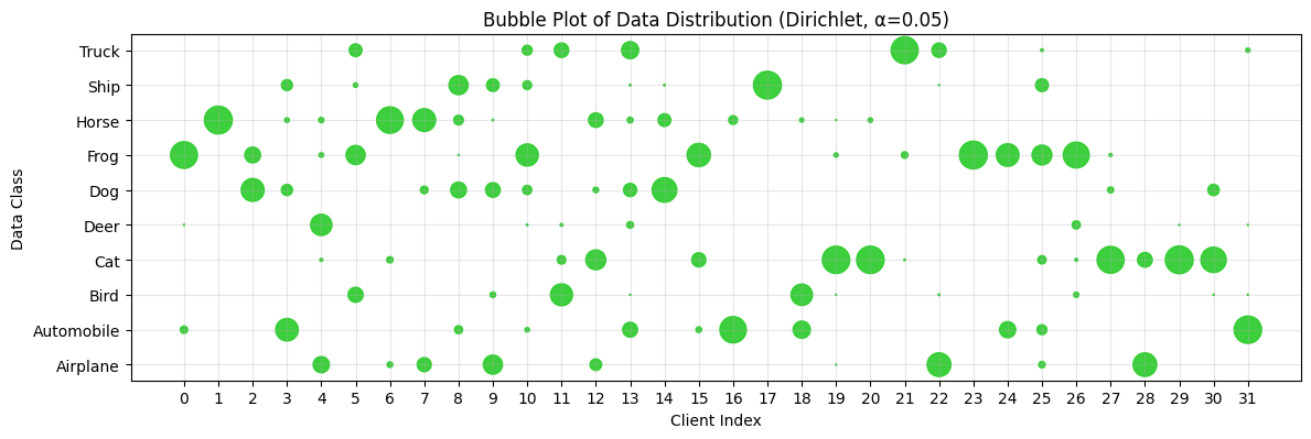
Figure 8: Dirichlet Data Distribution ($\alpha=0.05$)

E.2 Experiment Results of SG-FOCUS

From Figure 9, we observe that under highly heterogeneous data distribution ($\alpha=0.05$) and arbitrary client participation/sampling, our SG-FOCUS shows the best performance on convergence speed and test accuracy, compared to FedAU and SCAFFOLD. These results echo the view in our main paper: SG-FOCUS can jointly handle both data heterogeneity and arbitrary client participation.

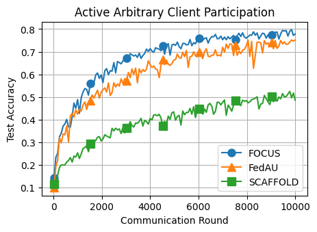
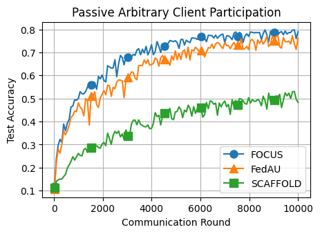
Figure 9: Performance Comparison of SG-FOCUS and Baselines on CIFAR10 Dataset under Arbitrary Client Participation and High Data Heterogeneity.

References

- Assran et al. [2019] Mahmoud Assran, Nicolas Loizou, Nicolas Ballas, and Mike Rabbat. Stochastic gradient push for distributed deep learning. In International Conference on Machine Learning, pages 344–353. PMLR, 2019.
- Beltrán et al. [2023] Enrique Tomás Mart\́boldsymbol{i}nez Beltrán, Mario Quiles Pérez, Pedro Miguel Sánchez Sánchez, Sergio López Bernal, Gérôme Bovet, Manuel Gil Pérez, Gregorio Mart\́boldsymbol{i}nez Pérez, and Alberto Huertas Celdrán. Decentralized federated learning: Fundamentals, state of the art, frameworks, trends, and challenges. IEEE Communications Surveys & Tutorials, 2023.
- Cattivelli et al. [2008] Federico S Cattivelli, Cassio G Lopes, and Ali H Sayed. Diffusion recursive least-squares for distributed estimation over adaptive networks. IEEE Transactions on Signal Processing, 56(5):1865–1877, 2008.
- Chen and Sayed [2012] Jianshu Chen and Ali H Sayed. Diffusion adaptation strategies for distributed optimization and learning over networks. IEEE Transactions on Signal Processing, 60(8):4289–4305, 2012.
- Fang et al. [2024] Minghong Fang, Zifan Zhang, Hairi, Prashant Khanduri, Jia Liu, Songtao Lu, Yuchen Liu, and Neil Gong. Byzantine-robust decentralized federated learning. In Proceedings of the 2024 on ACM SIGSAC Conference on Computer and Communications Security, pages 2874–2888, 2024.
- Johnson and Zhang [2013] Rie Johnson and Tong Zhang. Accelerating stochastic gradient descent using predictive variance reduction. Advances in neural information processing systems, 26, 2013.
- Kairouz et al. [2021] Peter Kairouz, H Brendan McMahan, Brendan Avent, Aurélien Bellet, Mehdi Bennis, Arjun Nitin Bhagoji, Kallista Bonawitz, Zachary Charles, Graham Cormode, Rachel Cummings, et al. Advances and open problems in federated learning. Foundations and trends® in machine learning, 14(1–2):1–210, 2021.
- Karimireddy et al. [2020] Sai Praneeth Karimireddy, Satyen Kale, Mehryar Mohri, Sashank Reddi, Sebastian Stich, and Ananda Theertha Suresh. Scaffold: Stochastic controlled averaging for federated learning. In International conference on machine learning, pages 5132–5143. PMLR, 2020.
- Koloskova et al. [2020] Anastasia Koloskova, Nicolas Loizou, Sadra Boreiri, Martin Jaggi, and Sebastian Stich. A unified theory of decentralized sgd with changing topology and local updates. In International Conference on Machine Learning, pages 5381–5393. PMLR, 2020.
- Krizhevsky et al. [2009] Alex Krizhevsky, Geoffrey Hinton, et al. Learning multiple layers of features from tiny images. 2009.
- Lalitha et al. [2018] Anusha Lalitha, Shubhanshu Shekhar, Tara Javidi, and Farinaz Koushanfar. Fully decentralized federated learning. In Third workshop on bayesian deep learning (NeurIPS), volume 2, 2018.
- Lan et al. [2020] Guanghui Lan, Soomin Lee, and Yi Zhou. Communication-efficient algorithms for decentralized and stochastic optimization. Mathematical Programming, 180(1):237–284, 2020.
- Li et al. [2020] Tian Li, Anit Kumar Sahu, Ameet Talwalkar, and Virginia Smith. Federated learning: Challenges, methods, and future directions. IEEE signal processing magazine, 37(3):50–60, 2020.
- Li et al. [2019a] Xiang Li, Kaixuan Huang, Wenhao Yang, Shusen Wang, and Zhihua Zhang. On the convergence of fedavg on non-iid data. arXiv preprint arXiv:1907.02189, 2019a.
- Li et al. [2024] Zhe Li, Bicheng Ying, Zidong Liu, Chaosheng Dong, and Haibo Yang. Achieving dimension-free communication in federated learning via zeroth-order optimization. arXiv preprint arXiv:2405.15861, 2024.
- Li et al. [2019b] Zhi Li, Wei Shi, and Ming Yan. A decentralized proximal-gradient method with network independent step-sizes and separated convergence rates. IEEE Transactions on Signal Processing, 67(17):4494–4506, 2019b.
- Lian et al. [2017] Xiangru Lian, Ce Zhang, Huan Zhang, Cho-Jui Hsieh, Wei Zhang, and Ji Liu. Can decentralized algorithms outperform centralized algorithms? a case study for decentralized parallel stochastic gradient descent. Advances in neural information processing systems, 30, 2017.
- McMahan et al. [2017] Brendan McMahan, Eider Moore, Daniel Ramage, Seth Hampson, and Blaise Aguera y Arcas. Communication-efficient learning of deep networks from decentralized data. In Artificial intelligence and statistics, pages 1273–1282. PMLR, 2017.
- Mishchenko et al. [2022] Konstantin Mishchenko, Grigory Malinovsky, Sebastian Stich, and Peter Richtárik. Proxskip: Yes! local gradient steps provably lead to communication acceleration! finally! In International Conference on Machine Learning, pages 15750–15769. PMLR, 2022.
- Nedić and Olshevsky [2014] Angelia Nedić and Alex Olshevsky. Distributed optimization over time-varying directed graphs. IEEE Transactions on Automatic Control, 60(3):601–615, 2014.
- Nedic and Ozdaglar [2009] Angelia Nedic and Asuman Ozdaglar. Distributed subgradient methods for multi-agent optimization. IEEE Transactions on Automatic Control, 54(1):48–61, 2009.
- Nedic et al. [2017] Angelia Nedic, Alex Olshevsky, and Wei Shi. Achieving geometric convergence for distributed optimization over time-varying graphs. SIAM Journal on Optimization, 27(4):2597–2633, 2017.
- Pu et al. [2020] Shi Pu, Wei Shi, Jinming Xu, and Angelia Nedić. Push–pull gradient methods for distributed optimization in networks. IEEE Transactions on Automatic Control, 66(1):1–16, 2020.
- Ryu and Yin [2022] Ernest K Ryu and Wotao Yin. Large-scale convex optimization: algorithms & analyses via monotone operators. Cambridge University Press, 2022.
- Saadatniaki et al. [2020] Fakhteh Saadatniaki, Ran Xin, and Usman A Khan. Decentralized optimization over time-varying directed graphs with row and column-stochastic matrices. IEEE Transactions on Automatic Control, 65(11):4769–4780, 2020.
- Sayed et al. [2014] Ali H Sayed et al. Adaptation, learning, and optimization over networks. Foundations and Trends® in Machine Learning, 7(4-5):311–801, 2014.
- Shi et al. [2015] Wei Shi, Qing Ling, Gang Wu, and Wotao Yin. Extra: An exact first-order algorithm for decentralized consensus optimization. SIAM Journal on Optimization, 25(2):944–966, 2015.
- Shi et al. [2023] Yifan Shi, Li Shen, Kang Wei, Yan Sun, Bo Yuan, Xueqian Wang, and Dacheng Tao. Improving the model consistency of decentralized federated learning. In International Conference on Machine Learning, pages 31269–31291. PMLR, 2023.
- Stich [2018] Sebastian U Stich. Local sgd converges fast and communicates little. arXiv preprint arXiv:1805.09767, 2018.
- Wang et al. [2024] Lin Wang, YongXin Guo, Tao Lin, and Xiaoying Tang. Delta: Diverse client sampling for fasting federated learning. Advances in Neural Information Processing Systems, 36, 2024.
- Wang and Ji [2022] Shiqiang Wang and Mingyue Ji. A unified analysis of federated learning with arbitrary client participation. Advances in Neural Information Processing Systems, 35:19124–19137, 2022.
- Wang and Ji [2023] Shiqiang Wang and Mingyue Ji. A lightweight method for tackling unknown participation statistics in federated averaging. arXiv preprint arXiv:2306.03401, 2023.
- Xiang et al. [2024] Ming Xiang, Stratis Ioannidis, Edmund Yeh, Carlee Joe-Wong, and Lili Su. Efficient federated learning against heterogeneous and non-stationary client unavailability. arXiv preprint arXiv:2409.17446, 2024.
- Xin and Khan [2018] Ran Xin and Usman A Khan. A linear algorithm for optimization over directed graphs with geometric convergence. IEEE Control Systems Letters, 2(3):315–320, 2018.
- Ying et al. [2021] Bicheng Ying, Kun Yuan, Yiming Chen, Hanbin Hu, Pan Pan, and Wotao Yin. Exponential graph is provably efficient for decentralized deep training. Advances in Neural Information Processing Systems, 34:13975–13987, 2021.
- Yuan et al. [2016] Kun Yuan, Qing Ling, and Wotao Yin. On the convergence of decentralized gradient descent. SIAM Journal on Optimization, 26(3):1835–1854, 2016.
- Yuan et al. [2018] Kun Yuan, Bicheng Ying, Xiaochuan Zhao, and Ali H Sayed. Exact diffusion for distributed optimization and learning—part i: Algorithm development. IEEE Transactions on Signal Processing, 67(3):708–723, 2018.