¹Department of Computer Science, Emory University, Atlanta, GA
²Department of Biostatistics and Bioinformatics, Emory University, Atlanta, GA

Higher-order Interaction Matters: Dynamic Hypergraph Neural Networks for Epidemic Modeling

Abstract

The ongoing need for effective epidemic modeling has driven advancements in capturing the complex dynamics of infectious diseases. Traditional models, such as Susceptible-Infected-Recovered, and graph-based approaches often fail to account for higher-order interactions and the nuanced structure pattern inherent in human contact networks. This study introduces a novel Human Contact-Tracing Hypergraph Neural Network framework tailored for epidemic modeling called EpiDHGNN, leveraging the capabilities of hypergraphs to model intricate, higher-order relationships from both location and individual level. Both real-world and synthetic epidemic data are used to train and evaluate the model. Results demonstrate that EpiDHGNN consistently outperforms baseline models across various epidemic modeling tasks, such as source detection and forecast, by effectively capturing the higher-order interactions and preserving the complex structure of human interactions. This work underscores the potential of representing human contact data as hypergraphs and employing hypergraph-based methods to improve epidemic modeling, providing reliable insights for public health decision-making.

1 Introduction

Since the onset of the COVID-19 pandemic, there has been a growing interest in studying epidemiological models^{1; 2; 3}. Understanding and managing infection outbreaks is crucial for public health. Traditional mechanistic models like Susceptible-Infected-Recovered (SIR), which mathematically describe the transmission mechanisms of infectious diseases, often suffer from limitations of oversimplified or fixed assumptions, leading to sub-optimal predictive power and inefficiency in capturing complex epidemic patterns ^{4; 5}.

Motivated by these limitations, sequential models such as GRU ⁶ and LSTM ⁷ are used to model temporal relations in a data-driven manner. Compared to mechanistic models, sequential models have demonstrated superior performance in forecasting infection counts ^{1; 8; 9}. However, these models often struggle to incorporate spatial dependencies, such as human mobility patterns and geographical distributions, which play a crucial role in epidemiology modeling ². Mobility data captures how individuals move and interact across different locations, influencing disease transmission dynamics beyond simple temporal trends. To enhance the ability to capture both spatial and temporal information, graph-based approaches have emerged as a popular tool in epidemic research. Graph Neural Networks (GNNs) ^{10; 11} have become popular for their ability to model human mobility patterns. They achieve this by representing nodes as regions and weighted edges as mobility volume, effectively capturing movement between locations. Through a message-passing mechanism, GNNs enable nodes to share information with their neighbors, allowing for a more comprehensive understanding of mobility patterns. Additionally, by leveraging dynamic graph modeling and dynamic GNNs, they can further represent changes in human movement over time, enhancing their ability to model relational dynamics within mobility networks. ^{12; 13; 5}

Despite the utility of GNN-based methods, they primarily focus on pair-wise interactions and therefore neglect the higher-order interactions that are inherent in actual human contact networks ^{14; 15; 16}. Specifically, higher-order interactions refer to interactions or contacts that involve more than two individuals simultaneously in the context of epidemic modeling ¹⁷. For example, public transportation, workplaces, and schools are shared spaces where groups of people interact following higher-order transmission dynamics. As illustrated in Figure 1, while standard graphs can model these interactions by representing individuals as nodes and forming fully connected subgraphs for each group, this approach is often inefficient and obscures the true higher-order structure. In contrast, hypergraphs provide a more natural and explicit way to represent higher-order interactions through hyperedges, eliminating the artificial clique. Additionally, hypergraphs can model overlapping interactions by representing locations as hyperedges, encompassing multiple individuals simultaneously. These enhancements can lead to more accurate and interpretable modeling of epidemics than standard graphs ^{14; 15; 18}.

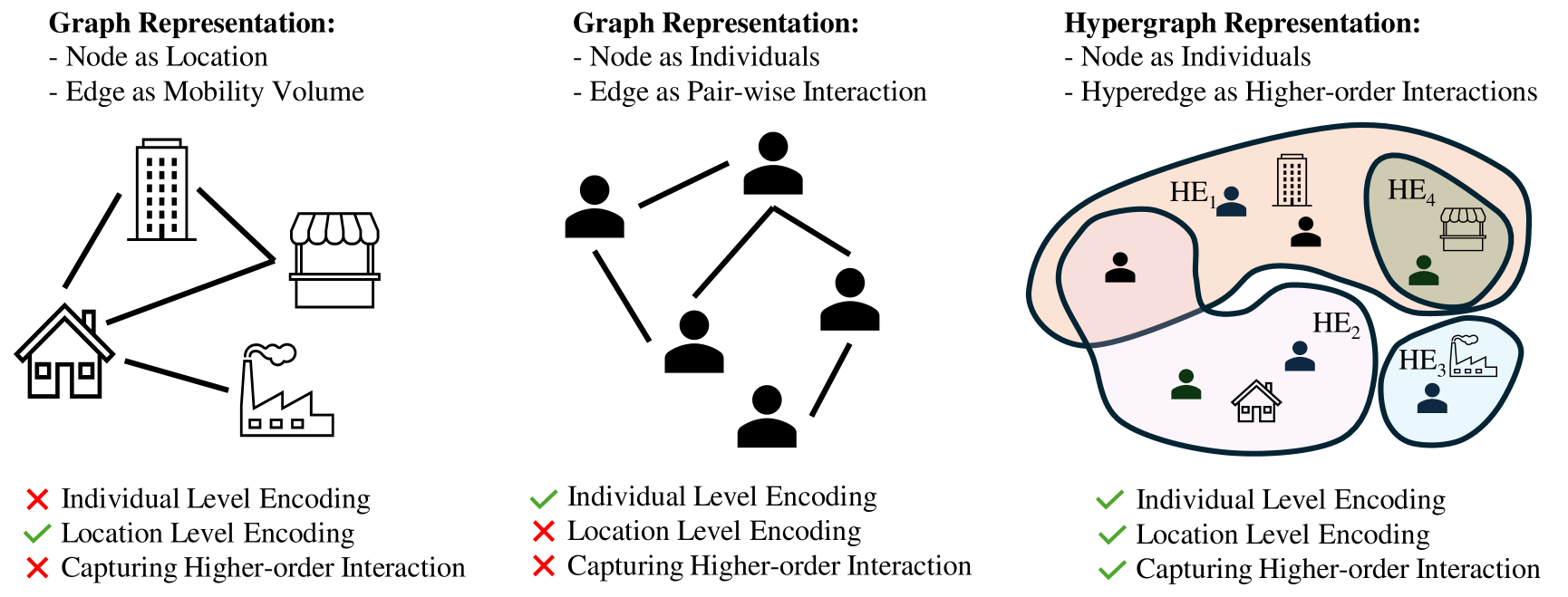
Figure 1: Illustration of how various graph encoding methods can be employed to capture complex interactions. Hypergraphs, in particular, offer significant advantages over traditional graphs by retaining both individual-level and location-level information, while also capturing higher-order interactions. This enriched representation facilitates a more nuanced understanding of epidemic dynamics.

As illustrated in Figure 1, a fundamental limitation of prior graph-based approaches lies in their inability to simultaneously preserve both individual-level and location-level information, as well as their failure to capture higher-order interactions. These shortcomings significantly hinder the accurate modeling of real-world human contact patterns, which are essential for understanding and predicting the spread of infectious diseases. To address this, we propose EpiDHGNN, a novel framework that models human contact data as dynamic hypergraphs. This approach enables the encoding of complex, higher-order interactions and supports a richer, more granular representation of epidemic dynamics. The major contributions of this paper are threefold:

1. We propose a novel method to model human contact as dynamic hypergraphs, which encodes nodes as individuals and hyperedges as locations, leveraging both granular level information and higher-order interactions.

2. We develop EpiDHGNN, a model tailor-made for epidemic modeling with a self-supervised contact-pattern awareness module, capturing the higher-order interactions and contact patterns that are inherent in human contacts.

3. Extensive experiments are conducted to demonstrate the superiority of encoding human contact as hypergraphs, as well as the effectiveness of our proposed models in various epidemic tasks.

2 Related Work

Mechanistic Epidemic Modeling: In the past, when data was not sufficiently recorded, scientists were unable to build empirical models that successfully captured the dynamics of epidemics. Empirical models rely heavily on accurate and comprehensive data to make predictions and understand patterns. In contrast, mechanistic models^{19; 20} are designed to capture the underlying complexity of infections and the recovery processes of various diseases, even with limited data. Among these, the compartmental model, exemplified by the Susceptible-Infectious-Recovered (SIR) model²¹, is considered one of the most popular and successful. The model divides the population into compartments based on their disease status, allowing for a structured and systematic analysis of epidemic progression. It uses two parameters, $\beta$ and $\gamma$, to account for the infection and recovery rates respectively. The model’ ability to incorporate epidemiological principles makes it particularly valuable for understanding and predicting the course of infectious diseases.

Graphs for Epidemic Modeling: Recent advancements in dynamic graph modeling have underscored the utility of such models in epidemic source detection and spread prediction. Initially developed for traffic forecasting, dynamic graph models have been rapidly adapted to epidemiological contexts, where nodes represent geographical locations.^{2; 5; 22; 23} However, these methods overlook the higher-order interaction inherent in human contact networks. Furthermore, previous works also focus on utilizing the dynamic message-passing (DMP) inference algorithm and network centrality as a tool for statistical inference to estimate the origin of an epidemic outbreak.^{24; 25; 14} Such algorithms iteratively transmit messages along network edges, updating each node’s state probabilities based on the states of its neighbors. However, they operate on static graphs, thereby overlooking the inherent dynamics of contact networks in human societies.

Hypergraphs for Epidemic Modeling: Similar to graphs, hypergraphs can be utilized in epidemic modeling while encompassing higher-order interactions. ^{26; 27; 28} In the pathogen propagation function proposed by Hypergraph-HeterSIS¹⁶, the infection state of each node is first aggregated to hyperedge, which is then followed by a nonlinear function $f$ to remove linearity. The result is then mapped back to node level to provide the next step update. The method has been shown that hypergraph-based approaches are better at capturing the structural differences in contact networks and improving the accuracy of infection dynamics modeling. However, these approaches are based on variable calibration, therefore neglecting the higher-level representation generated through deep learning approaches.^{15; 29; 30}

3 Formulation

3.1 Hypergrpah: A hypergraph is a higher-order representation of a graph where an edge can connect any number of vertices. Formally, a hypergraph $G=(V,\mathcal{E},\mathbf{X})$ consists of a set of nodes $V$, a set of hyperedges $\mathcal{E}$, where each hyperedge is a subset of $V$, and a feature matrix $\mathbf{X}\in\mathbb{R}^{|V|\times d}$, where each row encodes the node feature. The hypergraph structure can be described by an incidence matrix $\mathbf{H}\in\mathbb{R}^{|\mathcal{E}|\times N}$, where $\mathbf{H}_{i,j}=1$ only when the node $v_{i}$ is incident to the edge $e_{j}$.

3.2 Dynamic Hypergrpah: A dynamic hypergraph is an extension of a hypergraph that evolves over time, consisting of a sequence of hypergraphs observed over $T$ discrete time stamps. Formally, a dynamic hypergraph is represented as $G^{(0:T)}=\{G^{(0)},G^{(1)},\dots,G^{(T)}\}$, where each hypergraph $G^{(t)}=(V^{(t)},\mathcal{E}^{(t)},\mathbf{X}^{(t)})$ denotes the hypergraph at time stamp $t\in[0:T]$. Here, $V^{(t)}$ is the set of nodes, $\mathcal{E}^{(t)}$ is the set of hyperedges, and $\mathbf{X}^{(t)}$ denotes the node features at time $t$. It is worth noting that both the graph structure and node features are dynamic, since in some works, dynamic graphs have static features.

3.3 Epidemic Tasks: Consider an input of a dynamic hypergraph $G^{(0:T)}=\{G^{(0)},\dots,G^{(T)}\}$, where each node represents an individual and each hyperedge represents a location. At an arbitrary time stamp $t$, the nodes in a hyperedge $e^{(t)}\in\mathcal{E}^{(t)}$ represent a single contact between these entities. Each hypergraph $G^{(t)}$ is associated with an individual state matrix $\mathbf{X}^{(t)}\in\mathbb{R}^{N\times d}$, where $d$ is the feature dimension of the individual. For example, in the SIR setting, $d$ can consist of three dimensions, which correspond to the $\{\text{Suspected},\text{Infected},\text{Recovered}\}$ status of a specific individual.

Additionally, we define three time stamps to clarify the time interval of our downstream epidemic tasks. $[0:\text{tsh}]$ where tsh stands for Time Stamp Hidden; $[\text{tsh}:\text{ks}]$ where ks stands for Known Time Stamp; $[\text{ks}:\text{ps}]$ where ps stands for Prediction Time Stamp. The three time stamps are ordered such that $0\leq\text{tsh}\leq\text{ks}\leq\text{ps}\leq T$. Note that for a time stamp $t\in T$, when $t<\text{tsh}$, only contact hypergraph can be observed. When $\text{tsh}\leq t\leq\text{ks}$, both contact hypergraph and individual state can be observed. When $t>\text{ps}$, neither contact hypergraph nor individual state can be observed. An illustration of the three time stamps is shown in Figure 2.

3.3.1 Source Detection: The source detection task focuses on identifying the initial node responsible for the spread of an epidemic, often referred to as "patient zero." Given the dynamic hypergraph $G^{(0:\text{ks})}$, or its incidence matrix $\mathbf{H}^{(0:\text{ks})}$, and the corresponding state matrix $\mathbf{X}^{(\text{tsh}:\text{ks})}$, we aim to infer the likelihood distribution over all nodes at the initial time stamp $T=0$ using a model $f$ parametrized by weight $\theta$. Mathematically, we are interested in using $f_{\theta}$ to estimate the distribution:

$$f_{\theta}(\mathbf{H}^{(0:\text{ks})},\mathbf{X}^{(\text{tsh}:\text{ks})})\approx p(\mathbf{X}^{(0)}|\mathbf{H}^{(0:\text{ks})},\mathbf{X}^{(\text{tsh}:\text{ks})}).$$

This task leverages both the structural properties of the hypergraph and the temporal evolution of the feature maps to backtrack the probable origin of the epidemic. The node labels $y_{\text{detect}}$ are extracted from specific columns of $\mathbf{X}^{(0)}$ that represent the infection state — for example, the "infected" column in the case of the SIR model. To optimize the model, we’ll use weighted binary cross-entropy loss between the predictions and node labels $y_{\text{detect}}$, where $w_{1}=\frac{|V|}{|y_{\text{detect}}=1|}$ and $w_{0}=\frac{|V|}{|y_{\text{detect}}=0|}$

$$\mathcal{L}_{\text{detect}}(\theta)=-\frac{1}{|V|}\sum_{v\in V}\left[w_{1}y_{\text{detect}}\log(f_{\theta})+w_{0}(1-y_{\text{detect}})\log(1-f_{\theta}\right)],$$

3.3.2 Infection Forecasting: Forecasting tasks in epidemics are usually defined as finding the total number of infections and recoveries in a range of future time stamps. This is because previous approaches encode nodes as areas, neglecting the individual level information. On the other hand, when using human contact hypergraphs, we can deduce a more fine-grained forecasting on an individual level. Therefore, we treat our forecast task as a binary node classification task. The node labels are defined as whether a node is in the "infected" state. Using the SIR model as an example, each node can be in one of three states, and only when it is in the "infected" state does the label become True. Here we are interested in using a model $g$ parametrized by $\theta$ to estimate the distribution:

$$g_{\theta}(\mathbf{H}^{(0:\text{ks})},\mathbf{X}^{(\text{tsh}:\text{ks})})\approx p(\mathbf{X}^{(\text{ks}+1,\text{ps})}|\mathbf{H}^{(0:\text{ks})},\mathbf{X}^{(\text{tsh}:\text{ks})})$$

Similar to source detection, we’ll use the binary cross-entropy loss between the predictions and node labels $y_{\text{forecast}}$. The labels are extracted from specific columns of $\mathbf{X}^{(\text{ks}+1:\text{ps})}$ that represent the infection state, similar to source detection label extraction.

$$\mathcal{L}_{\text{forecast}}(\theta)=-\frac{1}{|V|}\sum_{v\in V}\left[y_{\text{forecast}}\log(g_{\theta})+(1-y_{\text{forecast}})\log(1-g_{\theta}\right)],$$

4 Method

In this section, we will formulate our proposed model EpiDHGNN, which serves as $f_{\theta}$ and $g_{\theta}$ defined in Section 3.3. Here we define $t\in T_{\text{interest}}$ where $T_{\text{interest}}$ is the corresponding input interval for $\mathbf{H}$ defined in Sections 3.3.1 and 3.3.2.

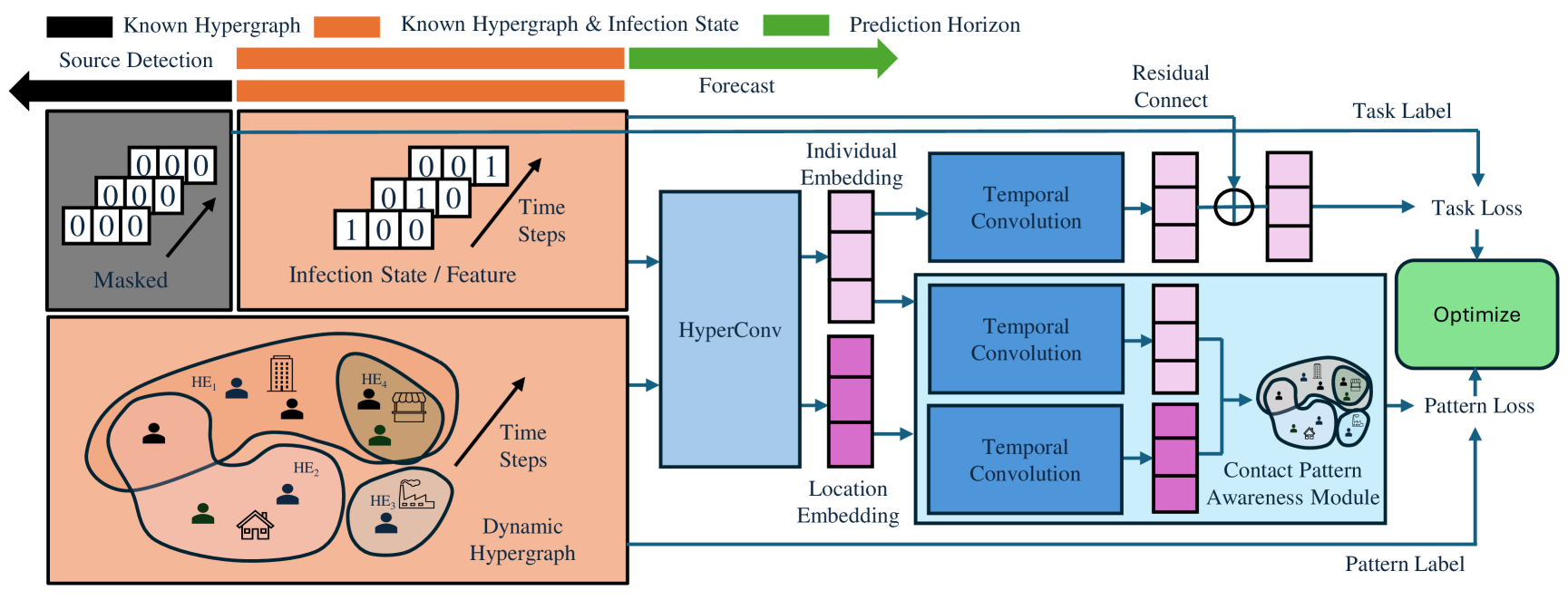
Figure 2: Model Architecture of proposed EpiDHGNN model. The arrows in the top left corner refers to the three time stamps defined in Section 3.3, where $[0:tsh]$ is the black interval, $[tsh:ks]$ is the orange interval, and $[ks+1:ps]$ is the green interval. All individual state is masked to 0 in $[0:tsh]$ as shown in the top left black module. Corresponding inputs for source detection and forecast defined in Section 3.3.1 and 3.3.2 is then feed to the model as input. The light blue HyperConv module in defined in Section 4.1; the dark blue temporal convolution module is defined in Section 4.1; and the contact pattern awareness module is defined in Section 4.2.

EpiDHGNN is a novel dynamic hypergraph neural network that models epidemic dynamics by jointly capturing spatial, temporal, and structural contact patterns. As illustrated in Figure 2, EpiDHGNN follows an encoder-decoder paradigm and integrates both supervised and self-supervised learning objectives to enhance the quality of node embeddings. The framework is composed of three key components: (1) a Spatial-Temporal Encoder based on hypergraph and temporal convolution that aggregates high-order relational information among individuals and captures progression patterns over time, (2) a novel self-supervised Contact Pattern Awareness Module that encourages structural consistency by reconstructing dynamic contact patterns. This architecture allows the model to learn robust spatiotemporal embeddings of infection states, improving performance on downstream tasks such as epidemic forecasting and source detection.

4.1 Spatio-Temporal Encoding: To capture spatial dependencies at each time step, we adopt the hypergraph convolution operator proposed in HGNN ¹⁵, which aggregates information from high-order neighbors via node-edge-node message passing. Formally, a single hypergraph convolutional layer consists of:

$$\mathbf{X}_{\text{edge}}^{l+1,t}=\mathbf{D}_{e}^{-1}\mathbf{H}^{T,t}\mathbf{D}_{v}^{-1/2}\mathbf{X}_{\text{node}}^{l,t}\Theta,$$ (1)

$$\mathbf{X}_{\text{node}}^{l+1,t}=\mathbf{D}_{v}^{-1/2}\mathbf{H}^{t}\mathbf{W}\mathbf{D}_{e}^{-1}\mathbf{H}^{T,t}\mathbf{D}_{v}^{-1/2}\mathbf{X}_{\text{node}}^{l,t}\Theta,$$ (2)

where $\mathbf{H}^{t}$ is the incidence matrix at time $t$, $\mathbf{D}_{v}$ and $\mathbf{D}_{e}$ are diagonal node and edge degree matrices, $\mathbf{W}$ is an optional hyperedge weighting matrix, and $\Theta$ denotes learnable parameters. By stacking $L$ such layers, the node embeddings can incorporate information from $L$-hop neighborhoods. After applying the convolution over all time steps, the node and edge embeddings are concatenated along the temporal axis:

$$\mathcal{X}_{\text{node}}^{L}=[\mathbf{X}_{\text{node}}^{L,t_{0}}\mid\mathbf{X}_{\text{node}}^{L,t_{1}}\mid\ldots],\quad\mathcal{X}_{\text{edge}}^{L}=[\mathbf{X}_{\text{edge}}^{L,t_{0}}\mid\mathbf{X}_{\text{edge}}^{L,t_{1}}\mid\ldots],\quad\forall t\in T_{\text{interest}}.$$ (3)

To capture temporal dependencies, we apply standard 1D convolution across the temporal axis, similar to the temporal convolutional networks introduced in ³¹ and later adapted for dynamic graphs in ³². Letting time correspond to the width dimension, individuals to the height, and feature channels to the depth, the operation is defined as:

$$\hat{\mathbf{X}}_{\text{node}}=\sigma\left(\Phi_{\text{temporal}}^{k}\circledast\mathcal{X}_{\text{node}}^{L}\right),$$ (4)

where $\circledast$ denotes convolution, $\Phi_{\text{temporal}}^{k}$ is the convolution kernel of width $k$, and $\sigma$ is a non-linear activation function. This enables the model to learn progression patterns across time.

4.2 Self-supervised Contact Pattern Awareness Module: In a societal setting, human interactions occur with varying probabilities based on social structures and daily routines. For instance, individuals are highly likely to engage in frequent interactions with family members or colleagues at home or in the workplace, while social encounters with friends or individuals sharing similar interests may occur less frequently, such as on a weekly or monthly basis in clubs or shopping centers. To leverage this information, we propose a self-supervised Contact Pattern Awareness Module, designed to predict human interactions within the epidemic framework. Given a sequence of $k$ hypergraphs $\{G_{t}\}_{t=t_{0}}^{t_{0}+k-1}$ starting from a randomly selected time step $t_{0}$, the module aims to reconstruct the hypergraph at the final time step, $G_{t_{0}+k}$, using information from the preceding $k-1$ hypergraphs. Successful reconstruction enables HGNN to inject human-contact-aware inductive bias into the learned node embeddings $\mathcal{X}_{\text{node}}^{L}$, thereby improving performance in subsequent epidemic forecasting tasks.

To effectively capture these patterns, we utilize both the individual embeddings and location embeddings obtained from Section 4.1. These embeddings are then processed using the temporal convolution framework introduced in Section 4.2, enabling the model to extract temporal dependencies. Finally, the refined embeddings are passed through a fully connected layer to produce a confidence score for contact prediction. Mathematically, this operation is formulated as:

$$\mathbf{s}=\sigma\left(\text{MLP}\left(\Phi_{\text{pattern}}^{k}\circledast\mathcal{X}_{\text{node}}^{L}*\Phi_{\text{pattern}}^{k}\circledast\mathcal{X}_{\text{edge}}^{L}\right)\right),$$ (5)

where $*$ denotes element-wise multiplication and $\sigma$ is a sigmoid activation. The output $\mathbf{s}$ is a predicted score for individual-location contact. The module is trained with binary cross-entropy loss on a balanced set of positive (observed) and negative (random) samples:

$$\mathcal{L}_{\text{pattern}}=-\frac{1}{N}\sum_{i=1}^{N}\left[y_{i}\log s_{i}+(1-y_{i})\log(1-s_{i})\right],$$ (6)

where $y_{i}\in\{0,1\}$ is the ground-truth label indicating whether contact occurred.

4.3 EpiDHGNN: Given an input sequence of dynamic hypergraphs $\{\mathbf{H}^{t}\}_{t=t_{0}}^{t_{0}+ks}$ and the corresponding individual features $\{\mathbf{X}^{t}\}_{t=t_{0}}^{t_{0}+ks}$, EpiDHGNN first encodes node representations using the spatial and temporal modules (Sections 4.1), and then incorporates initial state residuals before calculating task-specific loss. The overall loss is a combination of task-specific supervision and the self-supervised contact pattern loss:

$$\mathcal{L}=\alpha~\mathcal{L}_{\text{task}}+(1-\alpha)\mathcal{L}_{\text{pattern}},$$ (7)

where $\alpha$ is a weighting hyperparameter that balances predictive accuracy and structural awareness.

5 Experiment

In this section, we perform analysis on the datasets and conduct experiments to evaluate the proposed model. We will focus on the following research questions:

1. RQ1: Does EpiDHGNN outperforms baseline dynamic graph models in various epidemic tasks?

2. RQ2: Does the contact pattern awareness module facilitate the overall performance of EpiDHGNN?

3. RQ3: Is contact patterns successfully captured? To what aspect of the task does the module helps the most?

4. RQ4: Beyond individual-level prediction, can EpiDHGNN capture population-level infection dynamics over time?

Table 1: Dataset Summary

Metric	UVA	EpiSim
Individuals	2,500	10,000
Locations	500	11
Time Steps	169	47
Contacts	94,134	664,177

Data Description: We assess the performance of baseline models and our proposed model on both graphs and hypergraphs settings. Because of the privacy nature of human contact data, we used both real-world and synthetic data. The University of Virginia UVA dataset includes an extensive collection of clinical metadata sourced from the Epic-based SQL database at the UVA hospital. The interactions are derived from Electronic Healthcare Records (EHRs), which document the timing and locations of encounters between patients and healthcare workers (HCWs). We utilized the real-world infection case calibrated pathogen parameters provided by Anand etc. ¹⁶ to retrieve the patient infection states through simulations. The EpiSim dataset is based on the Mobility Intervention of Epidemic’s Simulator³³, which models human movement and disease transmission. The Human Mobility Model simulates hourly movements from 8 A.M. to 10 P.M. On weekdays, individuals move from residential to work areas at time $T_{d}\sim U(a,b)$, stay for $T_{w}\sim U(c,d)$ hours, and may visit commercial areas before returning home. On weekends, they visit commercial areas at $T_{e}\sim U(g,h)$ with probability $P_{e}$, staying for $T_{m}\sim U(i,j)$ hours. The Disease Transmission Model includes acquaintance and stranger contacts. Each individual has fixed acquaintance contacts at home ($K_{r}\sim U(m,n)$) and work ($K_{w}\sim U(o,p)$). At each timestep, infection occurs with probability $P_{a}$ from acquaintances and $P_{s}$ from strangers. The simulator parameters are calibrated using the Covid-19 $R_{0}$ from WHO. The statistics for both datasets are shown in Table 1.

Table 2: Experiment Result of Forecast Task. Best Performance under each setting is bolded.

		UVA		EpiSim
	PS	F1	AUROC	F1	AUROC
STGCN	5	0.526 ± 0.022	0.714 ± 0.035	0.632 ± 0.036	0.816 ± 0.029
	10	0.343 ± 0.028	0.688 ± 0.010	0.473 ± 0.025	0.692 ± 0.043
	20	0.398 ± 0.031	0.655 ± 0.031	0.195 ± 0.073	0.593 ± 0.010
ASTGCN	5	0.544 ± 0.038	0.731 ± 0.060	0.624 ± 0.030	0.801 ± 0.005
	10	0.376 ± 0.013	0.692 ± 0.012	0.489 ± 0.014	0.712 ± 0.009
	20	0.367 ± 0.009	0.652 ± 0.011	0.154 ± 0.045	0.612 ± 0.025
MSTGCN	5	0.721 ± 0.063	0.846 ± 0.013	0.869 ± 0.084	0.895 ± 0.010
	10	0.401 ± 0.041	0.647 ± 0.012	0.502 ± 0.042	0.729 ± 0.020
	20	0.358 ± 0.024	0.617 ± 0.065	0.223 ± 0.035	0.658 ± 0.056
EpiDHGNN	5	0.712 ± 0.023	0.837 ± 0.019	0.918 ± 0.042	0.957 ± 0.065
	10	0.576 ± 0.012	0.750 ± 0.008	0.612 ± 0.001	0.874 ± 0.017
	20	0.454 ± 0.007	0.685 ± 0.008	0.298 ± 0.080	0.779 ± 0.071

Setup: In our experiment, we utilize a 2-layer HGNN to capture neighborhood information. We perform a grid search over key hyperparameters, including hidden dimensions, learning rate, weight decay, kernal size, and $\alpha$. During training, we employ the ADAM optimizer with weight decay and gradient clipping activated to stabilize gradient updates and prevent exploding gradients. Models are trained for up to 100 epochs, with early stopping activated if the validation loss does not improve for 10 consecutive epochs. The experiments are conducted on a single NVIDIA Tesla V100 GPU with 16 GB of memory. Training time per epoch averages around 5 seconds. To enhance reproducibility, random seeds are fixed for data splitting, model initialization, and optimization processes. We run the baselines using the package EpiLearn ³⁴.

RQ1 - Performance: Our experimental results for both source detection and forecasting are presented in Table 3 and Table 2, respectively, with the best performance under each setting highlighted in bold. We evaluated the models under diverse conditions to assess their robustness. For source detection, we masked timesteps of varying lengths (5, 10, and 20) to examine the models’ ability to backtrack across different scenarios. Similarly, we tested forecasting performance using prediction horizons of 5, 10, and 20 timesteps. In most settings, EpiDHGNN outperforms the majority of baseline graph-based models, underscoring the advantages of hypergraph-based approaches in epidemic modeling through capturing the high-order contact interaction.

Table 3: Experiment Result of Source Detection Task. Best performance under each setting is bolded.

	UVA				EpiSim
	TSH	MRR	Hit@1	Hit@3	MRR	Hit@1	Hit@3
STGCN	5	0.491 ± 0.056	0.300 ± 0.036	0.650 ± 0.057	0.242 ± 0.075	0.145 ± 0.052	0.282 ± 0.035
	10	0.462 ± 0.064	0.315 ± 0.074	0.633 ± 0.024	0.129 ± 0.039	0.100 ± 0.103	0.195 ± 0.052
	20	0.427 ± 0.033	0.175 ± 0.023	0.596 ± 0.078	0.111 ± 0.047	0.089 ± 0.042	0.163 ± 0.017
ASTGCN	5	0.501 ± 0.026	0.300 ± 0.078	0.650 ± 0.052	0.226 ± 0.036	0.167 ± 0.033	0.333 ± 0.042
	10	0.486 ± 0.046	0.250 ± 0.082	0.667 ± 0.022	0.141 ± 0.067	0.100 ± 0.027	0.133 ± 0.014
	20	0.416 ± 0.029	0.205 ± 0.058	0.650 ± 0.032	0.118 ± 0.087	0.076 ± 0.031	0.100 ± 0.087
MSTGCN	5	0.618 ± 0.026	0.417 ± 0.029	0.767 ± 0.076	0.333 ± 0.029	0.167 ± 0.032	0.400 ± 0.058
	10	0.561 ± 0.026	0.350 ± 0.050	0.733 ± 0.058	0.213 ± 0.058	0.100 ± 0.026	0.200 ± 0.019
	20	0.442 ± 0.029	0.150 ± 0.058	0.700 ± 0.052	0.192 ± 0.016	0.089 ± 0.100	0.193 ± 0.029
EpiDHGNN	5	0.704 ± 0.033	0.517 ± 0.076	0.917 ± 0.029	0.401 ± 0.074	0.200 ± 0.100	0.500 ± 0.100
	10	0.662 ± 0.005	0.500 ± 0.015	0.783 ± 0.029	0.218 ± 0.037	0.133 ± 0.058	0.167 ± 0.058
	20	0.582 ± 0.031	0.350 ± 0.026	0.765 ± 0.050	0.219 ± 0.061	0.100 ± 0.100	0.200 ± 0.100

RQ2 - Ablation: We conducted an ablation study on the contact pattern awareness module to investigate Question 2. As shown in Table 4, removing this module led to a noticeable decline in performance, indicating its crucial role in capturing individual contact patterns. The results suggest that incorporating individual contact behaviors enhances the model’s ability to encode social interactions more effectively, aligning with societal norms. This highlights the importance of modeling personalized contact dynamics in improving the overall predictive capability of our approach.

Table 4: Ablation study on contact pattern awareness module.

			UVA		EpiSim
		Setting	MRR	Hit@1	MRR	Hit@1
Detection	w/o CT module	tsh-5	0.692 ± 0.050	0.483 ± 0.104	0.381 ± 0.027	0.167 ± 0.058
		tsh-10	0.644 ± 0.032	0.467 ± 0.058	0.204 ± 0.020	0.100 ± 0.013
		tsh-20	0.558 ± 0.014	0.323 ± 0.029	0.197 ± 0.006	0.100 ± 0.100
	w/ CT module	tsh-5	0.704 ± 0.033	0.517 ± 0.076	0.401 ± 0.074	0.200 ± 0.100
		tsh-10	0.662 ± 0.005	0.500 ± 0.005	0.218 ± 0.037	0.133 ± 0.058
		tsh-20	0.582 ± 0.031	0.350 ± 0.058	0.219 ± 0.061	0.100 ± 0.092
			F1	AUROC	F1	AUROC
Forecast	w/o CT module	ps-5	0.709 ± 0.004	0.830 ± 0.003	0.891 ± 0.003	0.912 ± 0.007
		ps-10	0.571 ± 0.008	0.747 ± 0.006	0.513 ± 0.007	0.824 ± 0.005
		ps-20	0.439 ± 0.008	0.680 ± 0.004	0.253 ± 0.006	0.724 ± 0.009
	w/ CT module	ps-5	0.712 ± 0.023	0.837 ± 0.019	0.918 ± 0.042	0.957 ± 0.006
		ps-10	0.576 ± 0.012	0.750 ± 0.008	0.612 ± 0.001	0.874 ± 0.004
		ps-20	0.454 ± 0.007	0.685 ± 0.008	0.298 ± 0.080	0.779 ± 0.071

Table 5: Contact Pattern Prediction

	UVA		EpiSim
Quantile	Range	F1	Range	F1
1	[:6]	0.795	[:616]	0.997
2	[6:11]	0.773	[616:1788]	0.852
3	[11:19]	0.809	[1788:1847]	0.820
4	[19:]	0.841	[1847:]	0.639
Overall	—	0.804	—	0.827

RQ3 - Module Effectiveness: To investigate whether the contact pattern is successfully captured, we evaluate the module’s performance in predicting contact existence at the location level. Specifically, locations are divided into four quantiles based on their contact intensity. For example, in the EpiSim dataset, households exhibit lower contact intensity compared to recreational locations. For each quantile, we report the prediction accuracy along with the overall accuracy in Table 5. The results suggest that the overall contact pattern is successfully reconstructed. While the UVA dataset shows little correlation between contact intensity and accuracy, the EpiSim dataset exhibits a strong negative correlation. This observation aligns with the underlying assumptions of our dataset. The UVA dataset includes hospital contacts, which may fluctuate due to patient movement, whereas in the EpiSim dataset, locations with low contact intensity likely correspond to households, where visits occur with high frequency and regularity.

We further investigate the influence of the hyperparameter $\alpha$, selecting values from 0.3, 0.5, 0.7, 0.9, 1.0, to assess its impact on overall model performance. Lower values of $\alpha$ were not considered, as $\alpha=0.3$ already exhibited significantly diminished performance, failing to effectively capture the model’s main task. As shown in Figure 3, our results indicate that $\alpha$ has little correlation with the final performance, suggesting that it can be treated as a tunable hyperparameter for future studies.

Additionally, we observe that the model with a high timestep hidden state (TSH20) consistently outperforms other configurations when incorporating $\alpha$. This suggests that integrating contact pattern information is particularly beneficial for tasks requiring a longer temporal memory, as it helps the model better capture long-term dependencies in contact patterns. These findings highlight the importance of tuning $\alpha$ based on specific task requirements while reinforcing the advantage of incorporating contact-aware representations for long-horizon forecasting.

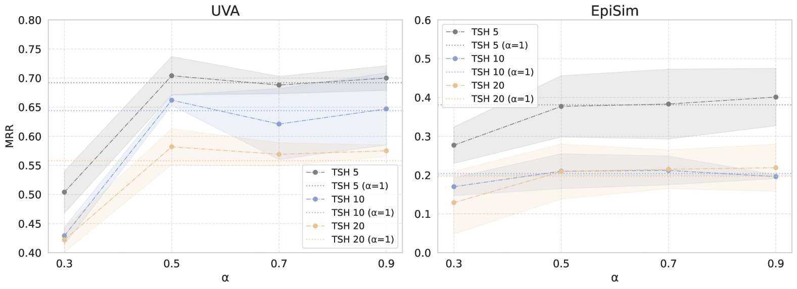
Figure 3: Visualization of various $\alpha$’s impact on source detection performance

RQ4 - Generalizability: While we have demonstrated EpiDHGNN’s ability to forecast an individual’s probability of infection in RQ1, its effectiveness at capturing the population infection trend cannot be concluded. To address this, we aggregated the daily sum of infected individuals to generate population-level data across various prediction horizons with respect to time. As shown in Figure 4, EpiDHGNN accurately captures short-term infection dynamics and effectively tracks broader fluctuations at longer time steps, albeit with reduced precision.

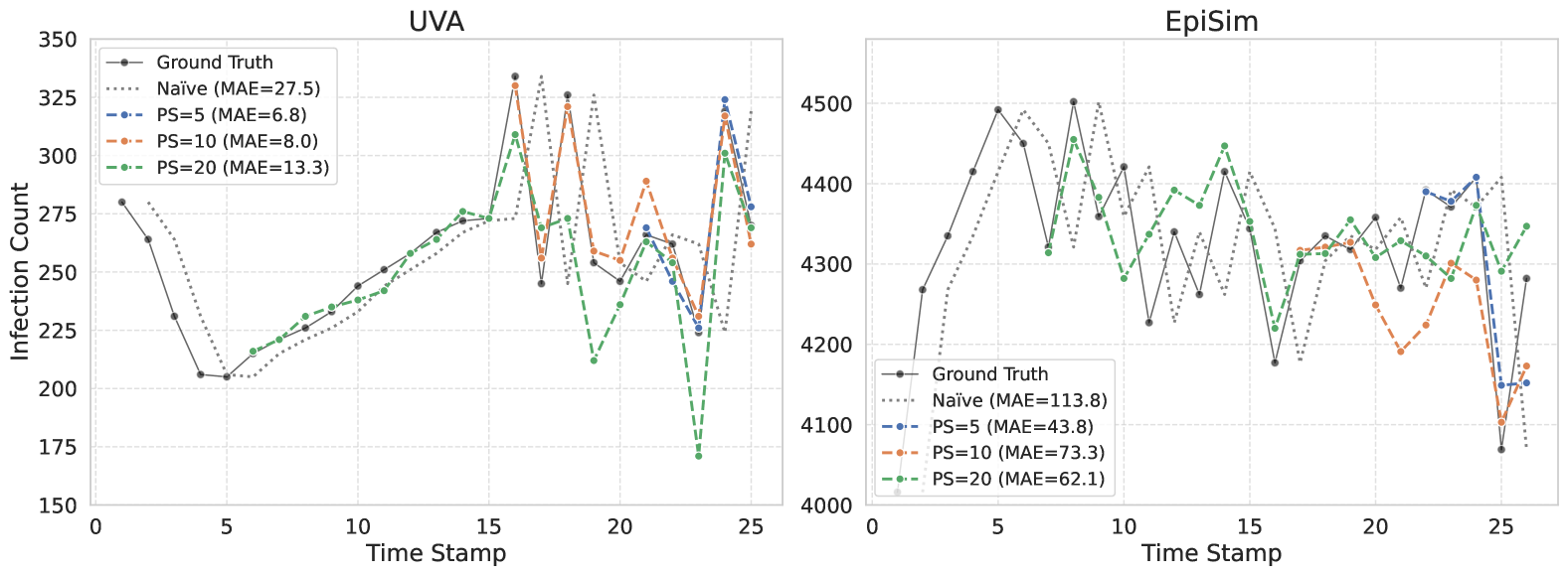
Figure 4: Forecast generalizability analysis. The models can successfully the future infection dynamics within various PS. We also provide the Mean Absolute Error (MAE) of Naive Model (A naive time series model forecasts future values by assuming they will be the same as the most recent observed value) and our method.

6 Discussion & Conclusion

This study introduced the EpiDHGNN framework, demonstrating its ability to effectively capture the dynamics of epidemic spread through higher-order interactions in human contact networks. Through rigorous experimentation on both real-world and synthetic datasets, we validated the advantages of modeling human contact as a dynamic hypergraph, highlighting the importance of higher-order relationships and contact pattern in disease transmission.

Future improvements include exploring alternative model selections within the EpiDHGNN framework, leveraging its modular design for flexible layer substitutions. Advanced architectures in hypergraph-based learning will be investigated to enhance accuracy and efficiency. Additionally, real-world simulation remains challenging due to privacy concerns and data scarcity. Developing realistic synthetic algorithms that capture social clustering, geographic mobility, and temporal dynamics will refine simulations, improve model training, and provide a stronger benchmark for epidemic modeling.

In summary, this work underscores the power of hypergraph-based epidemic modeling and sets the stage for further exploration into both methodological advancements and data generation strategies. By enabling more accurate identification of transmission dynamics, these models hold promise for informing timely and targeted public health interventions, ultimately contributing to more effective epidemic response strategies at a broader societal level.

References

- 1 Rodríguez A, Kamarthi H, Agarwal P, Ho J, Patel M, Sapre S, et al.. Data-Centric Epidemic Forecasting: A Survey; 2022. Available from: https://arxiv.org/abs/2207.09370.
- 2 Liu Z, Wan G, Prakash BA, Lau MSY, Jin W. A Review of Graph Neural Networks in Epidemic Modeling; 2024.
- 3 Clement JC, Ponnusamy V, Sriharipriya KC, Nandakumar R. A Survey on Mathematical, Machine Learning and Deep Learning Models for COVID-19 Transmission and Diagnosis. IEEE Reviews in Biomedical Engineering. 2022;15:325-40.
- 4 Song S, Zong Z, Li Y, Liu X, Yu Y. Reinforced Epidemic Control: Saving Both Lives and Economy; 2020.
- 5 Deng S, Wang S, Rangwala H, Wang L, Ning Y. Graph Message Passing with Cross-location Attentions for Long-term ILI Prediction; 2019. Available from: https://arxiv.org/abs/1912.10202.
- 6 Chung J, Gulcehre C, Cho K, Bengio Y. Empirical Evaluation of Gated Recurrent Neural Networks on Sequence Modeling; 2014.
- 7 Yu Y, Si X, Hu C, Zhang J. A review of recurrent neural networks: LSTM cells and network architectures. Neural computation. 2019;31(7):1235-70.
- 8 Rodríguez A, Cui J, Ramakrishnan N, Adhikari B, Prakash BA. EINNs: epidemiologically-informed neural networks. In: Proceedings of the AAAI conference on artificial intelligence. vol. 37; 2023. p. 14453-60.
- 9 Liu Z, Ni J, Lau MSY, Jin W. CAPE: Covariate-Adjusted Pre-Training for Epidemic Time Series Forecasting; 2025. Available from: https://arxiv.org/abs/2502.03393.
- 10 Yu B, Yin H, Zhu Z. Spatio-Temporal Graph Convolutional Networks: A Deep Learning Framework for Traffic Forecasting. In: Proceedings of the 27th International Joint Conference on Artificial Intelligence; 2018. p. 3634-40.
- 11 Liu H, Zhu C, Zhang D, Li Q. Attention-based Spatial-Temporal Graph Convolutional Recurrent Networks for Traffic Forecasting; 2023. Available from: https://arxiv.org/abs/2302.12973.
- 12 Zheng Y, Jiang W, Zhou A, Hung NQV, Zhan C, Chen T. Epidemiology-informed Graph Neural Network for Heterogeneity-aware Epidemic Forecasting; 2024. Available from: https://arxiv.org/abs/2411.17372.
- 13 Qiu M, Tan Z, Bao BK. MSGNN: Multi-scale Spatio-temporal Graph Neural Network for epidemic forecasting. Data Mining and Knowledge Discovery. 2024 May;38(4):2348–2376. Available from: http://dx.doi.org/10.1007/s10618-024-01035-w.
- 14 Tan CW, Yu PD. Contagion Source Detection in Epidemic and Infodemic Outbreaks: Mathematical Analysis and Network Algorithms. Foundations and Trends® in Networking. 2023;13(2–3):107–251. Available from: http://dx.doi.org/10.1561/1300000068.
- 15 Feng Y, You H, Zhang Z, Ji R, Gao Y. Hypergraph Neural Networks; 2019.
- 16 Anand V, Cui J, Heavey J, Vullikanti A, Prakash BA. In: H<sup>2</sup>ABM: Heterogeneous Agent-based Model on Hypergraphs to Capture Group Interactions; 2024. p. 280-8. Available from: https://epubs.siam.org/doi/abs/10.1137/1.9781611978032.32.
- 17 Kim S, Lee SY, Gao Y, Antelmi A, Polato M, Shin K. A survey on hypergraph neural networks: An in-depth and step-by-step guide. In: Proceedings of the 30th ACM SIGKDD Conference on Knowledge Discovery and Data Mining; 2024. p. 6534-44.
- 18 Cao Q, Jiang R, Yang C, Fan Z, Song X, Shibasaki R. MepoGNN: Metapopulation Epidemic Forecasting with Graph Neural Networks. In: Amini MR, Canu S, Fischer A, Guns T, Kralj Novak P, Tsoumakas G, editors. Machine Learning and Knowledge Discovery in Databases. Cham: Springer Nature Switzerland; 2023. p. 453-68.
- 19 Lessler J, Cummings DA. Mechanistic Models of Infectious Disease and Their Impact on Public Health. American Journal of Epidemiology. 2016 Mar;183(5):415-22. Epub 2016 Feb 17.
- 20 D’Agostino McGowan L, Grantz KH, Murray E. Quantifying Uncertainty in Mechanistic Models of Infectious Disease. American Journal of Epidemiology. 2021 Jan;190(7):1377–1385. Available from: http://dx.doi.org/10.1093/aje/kwab013.
- 21 Hethcote HW. The Mathematics of Infectious Diseases. SIAM Review. 2000;42(4):599-653.
- 22 Xie F, Zhang Z, Li L, Zhou B, Tan Y. EpiGNN: Exploring Spatial Transmission with Graph Neural Network for Regional Epidemic Forecasting; 2022. Available from: https://arxiv.org/abs/2208.11517.
- 23 Wan G, Liu Z, Lau MS, Prakash BA, Jin W. Epidemiology-aware neural ode with continuous disease transmission graph. arXiv preprint arXiv:241000049. 2024.
- 24 Lokhov AY, Mézard M, Ohta H, Zdeborová L. Inferring the Origin of an Epidemic with a Dynamic Message-Passing Algorithm. Phys Rev E. 2014;90(1):012801.
- 25 Yu PD, Tan CW, Fu HL. Epidemic Source Detection in Contact Tracing Networks: Epidemic Centrality in Graphs and Message-Passing Algorithms. IEEE Journal of Selected Topics in Signal Processing. 2022 feb;16(2):234-49. Available from: http://dx.doi.org/10.1109/JSTSP.2022.3153168.
- 26 Higham DJ, Kergorlay HLD. Disease extinction for susceptible-infected-susceptible models on dynamic graphs and hypergraphs. Chaos. 2022 8;32.
- 27 de Arruda GF, Petri G, Moreno Y. Social contagion models on hypergraphs. Phys Rev Res. 2020 Apr;2:023032. Available from: https://link.aps.org/doi/10.1103/PhysRevResearch.2.023032.
- 28 Ágnes Bodó, Katona GY, Simon PL. SIS epidemic propagation on hypergraphs; 2015.
- 29 Chien E, Pan C, Peng J, Milenkovic O. You are AllSet: A Multiset Function Framework for Hypergraph Neural Networks; 2022.
- 30 Agarwal S, Sawhney R, Thakkar M, Nakov P, Han J, Derr T. THINK: Temporal Hypergraph Hyperbolic Network. In: 2022 IEEE International Conference on Data Mining (ICDM). IEEE; 2022. p. 849-54.
- 31 Lea C, Vidal R, Reiter A, Hager GD. Temporal Convolutional Networks: A Unified Approach to Action Segmentation; 2016. Available from: https://arxiv.org/abs/1608.08242.
- 32 Guo S, Lin Y, Feng N, Song C, Wan H. Attention Based Spatial-Temporal Graph Convolutional Networks for Traffic Flow Forecasting. In: Proceedings of the AAAI Conference on Artificial Intelligence. vol. 33; 2019. p. 922-9.
- 33 Mobility Intervention of Epidemics; 2020. Accessed: 2025-02-13. Available from: https://hzw77-demo.readthedocs.io/en/latest/.
- 34 Liu Z, Li Y, Wei M, Wan G, Lau MSY, Jin W. EpiLearn: A Python Library for Machine Learning in Epidemic Modeling; 2024. Available from: https://arxiv.org/abs/2406.06016.