Quasi-Brittle Fracture: The Blended Approach

Abstract

A field theory is presented for predicting damage and fracture in quasi-brittle materials. The approach taken here is new and blends a non-local constitutive law with a two-point phase field. In this formulation, the material displacement field is uniquely determined by the initial boundary value problem. The theory naturally satisfies energy balance, with positive energy dissipation rate in accord with the Clausius-Duhem inequality. Notably, these properties are not imposed but follow directly from the constitutive law and evolution equation when multiplying the equation of motion by the velocity and integrating by parts. In addition to elastic constants, the model requires at most three key material parameters: the strain at the onset of nonlinearity, the ultimate tensile strength, and the fracture toughness. The approach simplifies parameter identification while ensuring representation of material behavior. The approach seamlessly handles fracture evolution across loading regimes, from quasi-static to dynamic, accommodating both fast crack propagation and quasi-brittle failure under monotonic and cyclic loading. Numerical simulations show quantitative and qualitative agreement with experiments, including three-point bending tests on concrete. The model successfully captures the cyclic load-deflection response of crack mouth opening displacement, the structural size-effect related to ultimate load and specimen size, fracture originating from corner singularities in L-shaped domains, and bifurcating fast cracks.

[1]organization=Department of Mathematics, Louisiana State University, addressline=Lockett Hall, city=Baton Rouge, postcode=70803-4918, state=LA, country=USA

1 Introduction

This paper presents a field theory to predict damage and fracture in quasi-brittle materials. The approach taken here is new and blends a non-local constitutive law with a two-point phase field, handling fracture evolution across quasi-static to dynamic loading regimes seamlessly. In this formulation, we establish an initial boundary value problem for which the material displacement field and damage field are shown to be uniquely determined. The damage field, which serves as the phase field for the problem, is exclusively a function of the material strain with values between zero and one. The energy balance between elastic potential energy and damage energy follows directly from the equations of motion, with positive energy dissipation rate in accordance with the Clausius-Duhem inequality. Moreover, the failure energy can be explicitly computed for a flat crack. Here, the failure energy factors into a product of two terms: one providing an explicit formula for the energy release rate, and the other giving the crack length. What is novel is that these properties are not imposed but follow directly from the constitutive law and evolution equations on multiplying the equation of motion by the velocity and integrating by parts. No assumptions beyond the evolution equation are required or used. Numerical simulations are developed using discrete approximations of the proposed model. In addition to elastic constants, the model requires at most three key material parameters: the strain at the onset of nonlinearity, the ultimate tensile strength, and the fracture toughness. The goal is to achieve an accurate representation of material behavior using the least number of parameters.

The space-time non-locality of the field theory presented here is motivated by the nonlocal computational models of free fracture given by peridynamics, Silling (2000), Silling et al. (2007), phase field methods, Bourdin et al. (2000), Aranson et al. (2000), Karma et al. (2001), Miehe et al. (2010), cohesive element modeling, Xu and Needleman (1994), and eigenerosion methods, Pandolfi and Ortiz (2012). In this approach, the force between pairs of points is related to the strain through a nonlinear constitutive law depending on the strain. Strains are calculated as difference quotients of displacements between pairs of points. Damage localization emerges solely from the dynamics through the two-point phase field, which assesses force degradation between pairs of points; see Figure 3 and (2.7). Unlike traditional phase field methods requiring an additional diffusive equation, our phase field and strain fields are directly coupled through nonlocal weighted averaging of pairwise interactions, similar to peridynamics, resulting in a single evolution equation in terms of the displacement field. In the blended approach, the critical energy release rate $\mathcal{G}_{c}$ follows from the evolution equations and is the energy per unit area needed to eliminate all tensile force interaction between points lying on either side of a straight crack. Direct mathematical analysis shows that this result is independent of the length scale of non-locality, see (6.21). However there remains an elastic resistance to compression across cracks, as shown in Section 2.2.

The proposed blended model handles quasi-brittle fracture across loading conditions, from quasi-static to dynamic fracture evolution, accommodating both monotonic and cyclic loading cases. We are motivated by earlier quasi-brittle models developed in peridynamics by Hobbs et al. (2022), Zaccariotto et al. (2015), Niazi et al. (2021), in the phase field models of Verhoosel and De Borst (2013), Wu (2017) and cohesive zone models Ortiz and Pandolfi (1999), Falk et al. (2001), Máirt´ın et al. (2014). The literature is vast and these citations are by no means exhaustive. Significantly, the deterministic size effect Bažant and Planas (1998) emerges directly from our initial boundary value problem and is observed in numerical simulations, consistent with size-effects reported by Hobbs et al. (2022) using an exponential peridynamic potential. We work with simple peridynamic two-point interactions to see for the simplest case that the blended approach recovers quasi-brittle phenomena including the size-effects and accurate load-displacement curves.

The solutions of the initial boundary value problem are obtained through numerical simulation and presented in Section 8. We begin with mode-I fracture simulations on a high-strength concrete beam under monotonic and cyclic loading. We then simulate mixed-mode fracture tests on concrete beams under cyclic loading. We follow with a mixed-mode fracture simulation for an L-shaped panel. We then examine fast fracture, exhibiting straight crack propagation and crack branching depending on the intensity of the loading. The section concludes by demonstrating the structural size effect for quasi-brittle fracture.

In conclusion, we deliver a well-posed boundary value problem for general degradation envelopes beyond bilinear, trilinear, and exponential, even envelopes allowing strain hardening before failure. In this paper, the material is assumed to be damaged under tensile stress; however, the approach proposed here extends without modification to include compressive damage. Future work will incorporate a broader array of continuum elastic effects using multi-point force potentials and interactions mediated by state-based peridynamic models, see Silling et al. (2007).

The paper is organized as follows: The initial boundary value problem for the fracture evolution of quasi-brittle material is formulated in the next section. The well-posedness of the fracture evolution problem then follows from the arguments of Section 3. Power and energy balance are established for load-controlled and displacement-controlled fracture evolutions in Sections 4 and 5. These results follow directly by multiplying the evolution equation by the velocity and integrating by parts. In section 6, it is shown that the model calibration follows directly from the two point interaction potential and energy balance and given values of elastic moduli, stress at which there is an onset of nonlinearity, strength, and energy release rate. Section 7 provides the dimension-free groups associated with the dynamics. The results of numerical experiments are presented in Section 8.

2 A nonlocal phase field formulation

The body containing the damaging material $\Omega$ is a bounded domain in two or three dimensions and has a characteristic length scale $L$. Nonlocal interactions between a point $\mathbf{x}$ and its neighbors $\mathbf{y}$ are confined to the sphere (disk) of radius $\epsilon$ denoted by $\mathcal{H}_{\epsilon}(\mathbf{x})=\{\mathbf{y}:\,|\mathbf{y}-\mathbf{x}|<\epsilon\}$. The length scale $\epsilon$ is taken to be significantly smaller than $L$ and small enough to resolve the process zone. Here $V^{\epsilon}_{d}=\omega_{d}\epsilon^{d}$ is the $d$ dimensional volume of the ball $\mathcal{H}_{\epsilon}(\mathbf{x})$ centered at $\mathbf{x}$ where $\omega_{d}$ is the volume of the unit ball in $d$ dimensions. The elastic displacement $\mathbf{u}(t,\mathbf{x})$ is defined for $0\leq t\leq T$ and $\mathbf{x}$ in $\Omega$. We write $\mathbf{u}(t)=\mathbf{u}(t,\cdot)$ and introduce the two point strain $S(\mathbf{y},\mathbf{x},\mathbf{u}(t))$ between the point $\mathbf{x}$ and any point $\mathbf{y}\in\mathcal{H}_{\epsilon}(\mathbf{x})$ resolved along direction $\mathbf{e}$ given by

$$S(\mathbf{y},\mathbf{x},\mathbf{u}(t))=\frac{(\mathbf{u}(t,\mathbf{y})-\mathbf{u}(t,\mathbf{x}))}{|\mathbf{y}-\mathbf{x}|}\cdot\mathbf{e}, \hbox{ where }\mathbf{e}=\frac{\mathbf{y}-\mathbf{x}}{|\mathbf{y}-\mathbf{x}|},$$ (2.1)

and introduce the scaled strain

$$r:=r(\mathbf{y},\mathbf{x},\mathbf{u}(t))=\sqrt{\frac{|\mathbf{y}-\mathbf{x}|}{L}}S(\mathbf{y},\mathbf{x},\mathbf{u}(t)).$$ (2.2)

The strain satisfies the symmetry $S(\mathbf{y},\mathbf{x},\mathbf{u}(t))=S(\mathbf{x},\mathbf{y},\mathbf{u}(t))$. The scaled nonlocal kernel is introduced and is given by

$$\rho^{\epsilon}(\mathbf{y},\mathbf{x})=\frac{{\chi_{\Omega}(\mathbf{y})}J^{\epsilon}(|\mathbf{y}-\mathbf{x}|)}{\epsilon V^{\epsilon}_{d}},$$ (2.3)

where $\chi_{\Omega}$ is the characteristic function of $\Omega$, $J^{\epsilon}(|\mathbf{y}-\mathbf{x}|)$ is the influence function, a positive function on the ball of radius $\epsilon$ centered at $\mathbf{x}$ and is radially decreasing taking the value $M$ at the center of the ball and $0$ for $|\mathbf{y}-\mathbf{x}|\geq\epsilon$. The radially symmetric influence function is written $J^{\epsilon}(|\mathbf{y}-\mathbf{x}|)=J(|\mathbf{y}-\mathbf{x}|/\epsilon)$. The nonlocal kernel is scaled by $\epsilon^{-1}(V_{d}^{\epsilon})^{-1}$ enabling the model to be characterized by, 1) the linear elastic shear $G$ and Lamé $\lambda$ moduli in regions away from the damage, 2) the critical energy release rate ${G}_{c}$ and, 3) the strength of the material, this is done in Section 6.

2.1 Constitutive laws, Initial Boundary Value problem

The maximum strain up to time is $t$ given by

$$S^{*}(t,\mathbf{y},\mathbf{x},\mathbf{u})=\max_{0\leq\tau\leq t}\{S(\mathbf{y},\mathbf{x},\mathbf{u}(\tau))\}.$$ (2.4)

and set

$$r^{\ast}:=r^{\ast}(t,\mathbf{y},\mathbf{x},\mathbf{u})=\sqrt{\frac{|\mathbf{y}-\mathbf{x}|}{L}}S^{*}(\mathbf{y},\mathbf{x},\mathbf{u}(t)).$$

(a)

(b)

Figure 1: (a) The profile $g(r)$ used in characterizing the failure envelope. (b) Bond stiffness on the failure envelope of unloading laws $g^{\prime}(r)$ given by dashed curve. The bond stiffness becomes nonlinear at $r^{L}$, exhibits strain hardening between $r^{L}$ and $r^{C}$ and goes smoothly to zero at $r^{F}$. Unloading laws are linear elastic with a softer stiffness controlled by the phase field and shown in blue. The bond offers zero tensile stiffness for bonds broken in tension (red), see Definition 2. However the bond continues to elastically resist negative strains. The bond stiffness given in (2.9), (2.10).

We introduce the envelope associated with the nonlinear (convex-concave) potential function $g(r)$ given by $\partial_{r}g(r)$, see Figure 1(b). The force between two points is a function of the scaled strain. In the blended model the force is characterized by a stiffness between two points. Initially the stiffness remains a constant value with tensile strain but becomes nonlinear when the tensile strain exceeds $S^{L}$, exhibits strain hardening between $S^{L}$ and $S^{C}$ and goes smoothly to zero at $S^{F}$. On the other hand the force between two points is given by a constant stiffness for compressive strain.

Definition 1 (Bond).

The interval with end points $\mathbf{y}$ and $\mathbf{x}$ are referred to as a bond.

The bond stiffness at the strains $S^{L}$, $S^{C}$, and $S^{F}$ depend on the scaled bond length $\sqrt{|\mathbf{y}-\mathbf{x}|/L}$ and are given by parameters $r^{L}$, $r^{C}$, and $r^{F}$ determined by the material and the method of calibration is described in Section 6. The associated strains are given by:

$$S^{L}= \frac{r^{L}}{\sqrt{|\mathbf{y}-\mathbf{x}|/L}}$$

$$S^{C}= \frac{r^{C}}{\sqrt{|\mathbf{y}-\mathbf{x}|/L}}$$

$$S^{F}= \frac{r^{F}}{\sqrt{|\mathbf{y}-\mathbf{x}|/L}}.$$ (2.5)

The square root dependence on relative bond length is introduced in the regularized bond model Lipton (2014), Lipton (2016) and provides the envelope for fast fracture in Lipton and Bhattacharya (2025).

On the envelope the present strain at time $t$ is the maximum strain and $r^{*}=r$ and the strain dependent bond stiffness is proportional to the slope of the linear unloading curve and is $\frac{\partial_{r^{*}}g(r^{*})}{r^{*}}$ and

$$\frac{\partial_{r}g(r)}{r}=\frac{\partial_{r^{*}}g(r^{*})}{r^{*}}.$$ (2.6)

For positive strain the slope is constant $\partial_{r}g(r)/r=\overline{\mu}$ in a neighborhood of $r=0$ and represents the undamaged bond it then decreases as the strain increases and is written

$$\frac{\partial_{r^{*}}g(r^{*})}{r^{*}}=\overline{\mu}\gamma(\mathbf{u})(\mathbf{y},\mathbf{x},t),$$

where the two point phase field satisfies $0\leq\gamma(\mathbf{u})(\mathbf{y},\mathbf{x},t)\leq 1$ and is given by

$$\gamma(\mathbf{u})(\mathbf{y},\mathbf{x},t)=\frac{(\overline{\mu})^{-1}\partial_{r^{*}}g(r^{*})}{r^{*}}.$$ (2.7)

For positive strains the constitutive relationship is defined by

$$\hbox{bond force per unit volume${}^{2}$}=\rho^{\epsilon}(\mathbf{y},\mathbf{x})\mu(\gamma(\mathbf{u})(\mathbf{y},\mathbf{x},t))S(\mathbf{y},\mathbf{x},\mathbf{u}(t))\boldsymbol{e}$$ (2.8)

with

$$\mu(\gamma(\mathbf{u})(\mathbf{y},\mathbf{x},t)):=\overline{\mu}\gamma(\mathbf{u})(\mathbf{y},\mathbf{x},t),$$ (2.9)

for negative strains bonds do not soften i.e.,

$$\mu(\gamma(\mathbf{u})(\mathbf{y},\mathbf{x},t))=\overline{\mu},$$ (2.10)

and

$$\hbox{bond force per unit volume${}^{2}$}=\rho^{\epsilon}(\mathbf{y},\mathbf{x})\overline{\mu}S(\mathbf{y},\mathbf{x},\mathbf{u}(t))\boldsymbol{e}.$$ (2.11)

Definition 2 (Broken Bond).

In this treatment we say a bond between two points $\mathbf{y}$ and $\mathbf{x}$ “fails in tension” or “broken in tension” if and only if its stiffness is $\mu(\gamma(\mathbf{u})(\mathbf{y},\mathbf{x},t)=0$ for positive strains and $\overline{\mu}$ for negative strains.

This notion of broken bond still allows the “bond” to resist compressive force, see Figure 1(b).

The stiffness $\overline{\mu}$ is calibrated to the undamaged material stiffness in Section 6.

Figure 2: $\gamma(\mathbf{u})(\mathbf{y},\mathbf{x},t))$. It is one for $r^{\ast}\leq r^{L}$ then decays to zero for $r^{L}<r^{\ast}(t,\mathbf{y},\mathbf{x},\mathbf{u})<r^{F}$.

As an example consider the bilinear envelope for positive strains. For this case $r^{L}=r^{C}$ and the envelope is given by

$$\partial_{r^{*}}g(r^{*})=\left\{\begin{array}[]{lc}\overline{\mu}r^{*},&r^{*}<r^{C},\\ \overline{\mu}r^{C}\frac{r^{F}-r^{*}}{r^{F}-r^{C}},&r^{C}\leq r^{*}\leq r^{F},\\ 0,&r^{F}<r^{*}.\end{array}\right.$$ (2.12)

Then the two point phase field is

$$\gamma(\mathbf{u})(\mathbf{y},\mathbf{x},t)=\left\{\begin{array}[]{lc}1,&r^{*}<r^{C},\\ (\frac{r^{F}}{r^{*}}-1)\frac{r^{C}}{(r^{F}-r^{C})},&r^{C}\leq r^{*}\leq r^{F},\\ 0,&r^{F}<r^{*}.\end{array}\right.$$ (2.13)

see Figure 2. As before the undamaged bond force per unit volume² is $\rho^{\epsilon}(\mathbf{y},\mathbf{x})\overline{\mu}S(\mathbf{y},\mathbf{x},\mathbf{u}(t))\mathbf{e}$ and no bonds damage for negative strains.

The set of bonds corresponding to negative two point strain is denoted $N^{\epsilon}(t)$ and is the collection of pairs $(\mathbf{x},\mathbf{y})$ in $\Omega\times(\Omega\cap\mathcal{H}_{\epsilon}(\mathbf{x}))$ such that the bond between them sustains negative strain is

$$N^{\epsilon}(t)=\{(\mathbf{x},\mathbf{y})\hbox{ in }\Omega\times(\Omega\cap\mathcal{H}_{\epsilon}(\mathbf{x}));\,S(\mathbf{y},\mathbf{x},\mathbf{u}(t))\leq 0\}$$ (2.14)

and has with indicator function

$$\chi_{N}:=\chi_{N}(S(\mathbf{y},\mathbf{x},\mathbf{u}(t)))=\left\{\begin{array}[]{ll}1,&\hbox{if $(\mathbf{x},\mathbf{y})$ in $N^{\epsilon}(t)$}\\ 0,&\hbox{otherwise}.\end{array}\right.$$ (2.15)

Similarly denote the collection of pairs $(\mathbf{x},\mathbf{y})$ in $\Omega\times(\Omega\cap\mathcal{H}_{\epsilon}(\mathbf{x}))$ such that the bond between them sustains non-negative strain by

$$P^{\epsilon}(t)=\{(\mathbf{x},\mathbf{y})\hbox{ in }\Omega\times(\Omega\cap\mathcal{H}_{\epsilon}(\mathbf{x}));\,S(\mathbf{y},\mathbf{x},\mathbf{u}(t))\geq 0\}.$$ (2.16)

This set has indicator function

$$\chi_{P}:=\chi_{P}(S(\mathbf{y},\mathbf{x},\mathbf{u}(t)))=\left\{\begin{array}[]{ll}1,&\hbox{if $(\mathbf{x},\mathbf{y})$ in $P^{\epsilon}(t)$}\\ 0,&\hbox{otherwise}.\end{array}\right.$$ (2.17)

Collecting definitions we have $\mu(\gamma(\mathbf{u})(\mathbf{y},\mathbf{x},t))$ defined for all strains and given by

$$\mu(\gamma(\mathbf{u})(\mathbf{y},\mathbf{x},t)):=\chi_{N}\overline{\mu}+\chi_{P}\mu(\gamma(\mathbf{u})(\mathbf{y},\mathbf{x},t))$$ (2.18)

In summary the constitutive law relating force to strain and subsequent bond failure in tension is described by

$$\boldsymbol{f}^{\epsilon}(t,\mathbf{y},\mathbf{x},\mathbf{u})=\rho^{\epsilon}(\mathbf{y},\mathbf{x})\mu(\gamma(\mathbf{u})(\mathbf{y},\mathbf{x},t))S(\mathbf{y},\mathbf{x},\mathbf{u}(t))\boldsymbol{e},$$ (2.19)

see Figure 3. The nonlocal force density $\mathcal{L}^{\epsilon}[\mathbf{u}](t,\mathbf{x})$ defined for all points $\mathbf{x}$ in $\Omega$ is given by

$$\mathcal{L}^{\epsilon}[\mathbf{u}](t,\mathbf{x})=-\int_{\Omega}\boldsymbol{f}^{\epsilon}(t,\mathbf{y},\mathbf{x},\mathbf{u})\,d\mathbf{y}.$$ (2.20)

The material is assumed to be homogeneous and the balance of linear momentum for each point $\mathbf{x}$ in the body $\Omega$ is given by

$$\rho\ddot{\mathbf{u}}(t,\mathbf{x})+\mathcal{L}^{\epsilon}[\mathbf{u}](t,\mathbf{x})=\mathbf{b}(t,\mathbf{x}),$$ (2.21)

where $\mathbf{b}(t,\mathbf{x})$ is a prescribed body force density and $\rho$ is is the mass density of the material. The linear momentum balance is supplemented with the initial conditions on the displacement and velocity given by

$$\mathbf{u}(0,\mathbf{x})=\mathbf{u}_{0}(\mathbf{x}),$$

$$\dot{\mathbf{u}}(0,\mathbf{x})=\mathbf{v}_{0}(\mathbf{x}),$$ (2.22)

and we look for a solution $\mathbf{u}(t,\mathbf{x})$ on a time interval $0<t<T$. This completes the problem formulation for the load controlled fracture evolution where the body force $\mathbf{b}(t,\mathbf{x})$ for $0\leq t\leq T$ is prescribed.

Figure 3: The constitutive law for a bond. The failure envelope is the black dashed curve. The linear unloading is blue. The slope of the linear unloading curve decreases when the bond strain at the present time is equal to its maximum over all earlier times. This is indicated by the arrows on the dashed curve. The force - strain constitutive law for a bond unable resist tension is red. All bonds are linear elastic under compressive strain.

The failure envelope for this model corresponds to $r=r^{\ast}$ and is given by

$$\hbox{ bond force per unit volume${}^{2}$}=\rho^{\epsilon}(\mathbf{y},\mathbf{x})\frac{\partial_{r}g(r(\mathbf{y},\mathbf{x},\mathbf{u}(t)))}{\sqrt{\frac{{\mathbf{y}-\mathbf{x}}}{L}}}\boldsymbol{e}$$ (2.23)

In this model bond force and bond strength depends upon bond length through $r^{*}$, see (2.7).

A displacement load can be prescribed on the boundary of the specimen $\Omega$. For the non-local model the displacement $\mathbf{U}(t,\mathbf{x})$ is prescribed on a layer $\Omega_{D}^{\epsilon}$ surrounding part or all of the specimen see, e.g., Du et al. (2015). We write $\Omega^{*}=\Omega\cup\Omega_{D}^{\epsilon}$ where the layer is of maximum thickness greater than or equal to $\epsilon$, see Figure 4 . With this in mind we write

$$\rho^{\ast,\epsilon}(\mathbf{y},\mathbf{x})=\frac{{\chi_{\Omega^{*}}(\mathbf{y})}J^{\epsilon}(|\mathbf{y}-\mathbf{x}|)}{\epsilon V^{\epsilon}_{d}},$$ (2.24)

and

$$\boldsymbol{f}^{\epsilon}(t,\mathbf{y},\mathbf{x},\mathbf{u})=\rho^{\ast,\epsilon}(\mathbf{y},\mathbf{x})\mu(\gamma(\mathbf{u})(\mathbf{y},\mathbf{x},t))S(\mathbf{y},\mathbf{x},\mathbf{u}(t))\boldsymbol{e},$$ (2.25)

with the nonlocal force density $\mathcal{L}^{\epsilon}[\mathbf{u}](t,\mathbf{x})$ defined for all points $\mathbf{x}$ in $\Omega$ given by

$$\mathcal{L}^{\epsilon}[\mathbf{u}](t,\mathbf{x})=-\int_{\Omega^{*}}\boldsymbol{f}^{\epsilon}(t,\mathbf{y},\mathbf{x},\mathbf{u})\,d\mathbf{y}.$$ (2.26)

For this case the initial boundary value problem for fracture evolution is to find a displacement $\mathbf{u}(t,\mathbf{x})$ on $\Omega^{*}$ that satisfies $\mathbf{u}(t,\mathbf{x})=\mathbf{U}(t,\mathbf{x})$ in $\Omega^{\epsilon}_{D}$ and for $\mathbf{x}$ in $\Omega$ satisfies the evolution equation

$$\rho\ddot{\mathbf{u}}(t,\mathbf{x})+\mathcal{L}^{\epsilon}[\mathbf{u}](t,\mathbf{x})=\mathbf{b}(t,\mathbf{x}),$$ (2.27)

for $0<t<T$, with the initial conditions on the displacement and velocity given by

$$\mathbf{u}(0,\mathbf{x})=\mathbf{u}_{0}(\mathbf{x}),$$

$$\dot{\mathbf{u}}(0,\mathbf{x})=\mathbf{v}_{0}(\mathbf{x}).$$ (2.28)

To illustrate ideas we fix all bonds crossing the interface between $\Omega$ and $\Omega^{\epsilon}_{D}$ to be undamaged and have stiffness $\overline{\mu}$ as well all bonds between points in $\Omega^{\epsilon}_{D}$.

2.2 Elastic Resistance to Compression Across a Crack

In this model cracks are created by bonds offering zero stiffness under tension. On the other hand bonds under compressive strains continue to resist elastically. When a bond ceases to resist tension the constitutive relation is illustrated by the red branch of the force strain relation in Figure 3. Let $\mathbf{n}$ denote the unit normal vector perpendicular to the crack. Let $\mathbf{y}-\mathbf{x}$ denote all line segments crossing a planar crack such that $(\mathbf{y}-\mathbf{x})\cdot\mathbf{n}>0$ and $\epsilon>|\mathbf{y}-\mathbf{x}|$. For deformation fields such that $(\mathbf{u}(t,\mathbf{y})-\mathbf{u}(t,\mathbf{x}))\|\mathbf{n}$ and $(\mathbf{u}(t,\mathbf{y})-\mathbf{u}(t,\mathbf{x}))\cdot\mathbf{n}<0$, basic geometric considerations show that the strain is compressive, ie., $S(\mathbf{y},\mathbf{x},\mathbf{u}(t))<0$ for all bonds $|\mathbf{y}-\mathbf{x}|<\epsilon$. The constitutive relation (2.10) shows that the bond force opposes the compressive strain for all bonds crossing the crack.

Figure 4: Domain $\Omega$ with prescribed Dirichlet data on $\Omega_{D}^{\epsilon}$. The union is denoted by $\Omega^{*}$

2.3 Damage evolution

We observe that nonlocal dynamics for $\mathbf{u}(t)$ over $\Omega$ in $\mathbb{R}^{d}$ presents as dynamics over

$$\{(\mathbf{y},\mathbf{x})\in\Omega\times\Omega\,;\,|\mathbf{y}-\mathbf{x}|<\epsilon\}\subset\mathbb{R}^{d}\times\mathbb{R}^{d}$$

for the two point strain $S(\mathbf{y},\mathbf{x},\mathbf{u}(t))$. In the next section we show that $\partial_{t}\gamma(\mathbf{u})(\mathbf{y},\mathbf{x},t)$ is well defined almost everywhere on $\Omega\times\Omega$, i.e., here $\mathbf{u}$ can have jumps in the $\mathbf{x}$ variable for $t$ fixed. The strain dynamics generates sets where force is related to strain and an evolution emerges for the phase field. The set of undamaged bonds at time $t$ is given by

$$UZ^{\epsilon}(t)=\{(\mathbf{y},\mathbf{x})\in\,\Omega\cup\Omega\,;\,|\mathbf{y}-\mathbf{x}|<\epsilon,\,\hbox{and}\,\,\gamma(\mathbf{u})(\mathbf{y},\mathbf{x},t))=1\hbox{ and }\partial_{t}\gamma(\mathbf{u})(\mathbf{y},\mathbf{x},t)=0\},$$ (2.29)

with indicator function

$$\chi_{UZ^{\epsilon}(t)}(\mathbf{y},\mathbf{x})=\left\{\begin{array}[]{ll}1,&\hbox{if $(\mathbf{y},\mathbf{x})$ in $UZ^{\epsilon}(t)$}\\ 0,&\hbox{otherwise}.\end{array}\right.$$ (2.30)

The set of pairs $(\mathbf{y},\mathbf{x})$ corresponding to damaged bonds but not yet irrevocably broken at time $t$ and are not damaging at time $t$ are given by the set

$$DZ^{\epsilon}(t) =\{(\mathbf{y},\mathbf{x})\in\,\Omega\cup\Omega\,;\,|\mathbf{y}-\mathbf{x}|<\epsilon,\,\hbox{and}\,\,1>\gamma(\mathbf{u})(\mathbf{y},\mathbf{x},t))>0\hbox{ and }\partial_{t}\gamma(\mathbf{u})(\mathbf{y},\mathbf{x},t)=0,\}$$ (2.31)

with indicator function

$$\chi_{DZ^{\epsilon}(t)}(\mathbf{y},\mathbf{x})=\left\{\begin{array}[]{ll}1,&\hbox{if $(\mathbf{y},\mathbf{x})$ in $DZ^{\epsilon}(t)$}\\ 0,&\hbox{otherwise}.\end{array}\right.$$ (2.32)

The set of bonds undergoing damage at time $t$ are given by the set

$$PZ^{\epsilon}(t) =\{(\mathbf{y},\mathbf{x})\in\,\Omega\cup\Omega\,;\,|\mathbf{y}-\mathbf{x}|<\epsilon,\,\hbox{and}\,\,\partial_{t}\gamma(\mathbf{u})(\mathbf{y},\mathbf{x},t)<0.\}$$ (2.33)

with indicator function

$$\chi_{PZ^{\epsilon}(t)}(\mathbf{y},\mathbf{x})=\left\{\begin{array}[]{ll}1,&\hbox{if $(\mathbf{y},\mathbf{x})$ in $PZ^{\epsilon}(t)$}\\ 0,&\hbox{otherwise}.\end{array}\right.$$ (2.34)

The failure set $\Gamma^{\epsilon}(t)$ is the collection of pairs $(\mathbf{y},\mathbf{x})$ in $\Omega\times\Omega$ such that $|\mathbf{y}-\mathbf{x}|<\epsilon$ and the bond between them was broken at some time $\tau$, $0<\tau\leq t$. The failure set is written

$$\Gamma^{\epsilon}(t)=\{(\mathbf{y},\mathbf{x})\hbox{ in }\Omega\times\Omega\,;\,|\mathbf{y}-\mathbf{x}|<\epsilon,\,\hbox{and}\,\,\gamma(\mathbf{u})(\mathbf{y},\mathbf{x},t)=0\}$$ (2.35)

with indicator function

$$\chi_{\Gamma^{\epsilon}(t)}(\mathbf{y},\mathbf{x})=\left\{\begin{array}[]{ll}1,&\hbox{if $(\mathbf{y},\mathbf{x})$ in $\Gamma^{\epsilon}(t)$}\\ 0,&\hbox{otherwise}.\end{array}\right.$$ (2.36)

Next we consider the jump set of the displacement $\mathbf{u}(t)$ along the direction $\mathbf{e}$ at time $t$ and introduce the relation between jump sets of $\mathbf{u}(t)$ and $\Gamma^{\epsilon}(t)$.

Definition 3 (Jump set).

$$J_{\mathbf{e}}^{+}(\mathbf{u}(t))=\{\mathbf{x}\in\Omega\,;\,\lim_{\mathbf{y}\rightarrow\mathbf{x}}(\mathbf{u}(t,\mathbf{y})-\mathbf{u}(t,\mathbf{x}))\cdot\mathbf{e}>0,\hbox{ for }(\mathbf{y}-\mathbf{x})\cdot\mathbf{e}>0,\hbox{ and }(\mathbf{y}-\mathbf{x})\|\mathbf{e}\}$$

It now follows that:

Lemma 1 (Relationship between jump discontinuities and bonds broken in tension).

If $\lim_{\mathbf{y}\rightarrow\mathbf{x}}S(\mathbf{y},\mathbf{x},\mathbf{u}(t))$ is positive and the displacement suffers a jump discontinuity at $\mathbf{x}$, then there exists an interval $(0,\eta)$ with $\epsilon\geq\eta>0$, for which the bonds $(\mathbf{x}+s\mathbf{e},\mathbf{x})$ with $0<s<\eta$ belong to $\Gamma^{\epsilon}(t)$, i.e., if $\mathbf{x}\in J_{\mathbf{e}}^{+}(\mathbf{u}(t))$ then $\mathbf{x}$ is the end point of the family of all broken bonds parallel to $\mathbf{e}$ of length less than $\eta$.

The lemma follows immediately from the definitions of $J^{+}_{\mathbf{e}}(\mathbf{u}(t))$ and $\Gamma^{\epsilon}(t)$.

The set of undamaged bonds at time $t$ is given by

$$UZ^{\epsilon}(t)=\{(\mathbf{x},\mathbf{y})\in\,\Omega\cup\Omega\cap\mathcal{H}_{\epsilon}(\mathbf{x})\hbox{ such that }\gamma(\mathbf{u})(\mathbf{y},\mathbf{x},t))=1\},$$

and the set of pairs $(\mathbf{y},\mathbf{x})$ corresponding to damaged and unloading but not yet irrevocably broken at time $t$ is given by the set

$$DZ^{\epsilon}(t) =\{(\mathbf{x},\mathbf{y})\in\,\Omega\cup\Omega\cap\mathcal{H}_{\epsilon}(\mathbf{x})\hbox{ such that }1>\gamma(\mathbf{u})(\mathbf{y},\mathbf{x},t))\geq 0,\hbox{ with }\partial_{t}\gamma(\mathbf{u})(\mathbf{y},\mathbf{x},t))=0.\}$$ (2.37)

The set of pairs $(\mathbf{y},\mathbf{x})$ currently in the process of damaging at time $t$ is the process zone and given by the set

$$PZ^{\epsilon}(t) =\{(\mathbf{x},\mathbf{y})\in\,\Omega\cup\Omega\cap\mathcal{H}_{\epsilon}(\mathbf{x})\hbox{ with }-\partial_{t}\gamma(\mathbf{u})(\mathbf{y},\mathbf{x},t))>0.\}$$

We show in Section 3 that this nonlinear nonlocal initial boundary problem can be solved and has a unique displacement - damage set pair.

3 Existence and uniqueness of displacement and damage evolution.

In this section we state and prove existence of solution for the force controlled fracture evolution. We then state the existence of solution for the general initial boundary value problem noting its proof follows methods identical to the force controlled problem. Body forces are easily chosen for which one can find a unique solution $\mathbf{u}(t,\mathbf{x})$ of the initial value problem in (2.21) and (2.22). We introduce the subspace $\mathcal{U}$ of rigid body motions defined by (3.1).

$$\mathcal{U}=\{\mathbf{w}:\,\mathbf{w}=\mathbb{Q}\mathbf{x}+\mathbf{c};\,\mathbb{Q}\in\mathbb{R}^{d\times d},\,\,\mathbb{Q}^{T}=-\mathbb{Q};\,\,\mathbf{c}\in\mathbb{R}^{d}\}.$$ (3.1)

Calculation shows $S(\mathbf{y},\mathbf{x},\mathbf{w})=0$ for $\mathbf{w}\in\mathcal{U}$, which is the null space of the strain operator. We require $\int_{\Omega}\mathbf{w}\cdot\mathbf{b}\,d\mathbf{x}=0$ for all $\mathbf{w}\in\mathcal{U}$ to guarantee solvability. We denote the subspace of $L^{\infty}(\Omega;\mathbb{R}^{d})$ orthogonal to $\mathcal{U}$ as $\dot{L}^{\infty}(\Omega;\mathbb{R}^{d})$ and to expedite the presentation we denote $\dot{L}^{\infty}(\Omega;\mathbb{R}^{d})$ by $X$. The norm on $C^{2}([0,T];X)$ is given by (3.2).

$$\|\mathbf{u}(t,\mathbf{x})\|_{C^{2}([0,T];X)}=\sup_{0\leq t\leq T}\{\sum_{i=0}^{2}||\partial_{t}^{i}\mathbf{u}(t,\mathbf{x})||_{X}\}.$$ (3.2)

To simplify notation, we denote the space $C([0,T];X)$ as $CX$ with the corresponding norm $\|\cdot\|_{CX}$. Similarly, we write $C^{2}([0,T];X)$ as $C^{2}X$. Existence and uniqueness of the solution is stated below.

Theorem 1 (Existence and Uniqueness of Solution of Force Controlled Fracture Evolution).

The initial value problem given by (2.21) and (2.22) with initial data in $X$ and $\mathbf{b}(t,\mathbf{x})$ belonging to $CX$ has a unique solution $\mathbf{u}(t,\mathbf{x})$ in $C^{2}X$ with two strong derivatives in time.

The initial value problem delivers a unique displacement-damage set pair: ${\mathbf{u}^{\epsilon}(t),DZ^{\epsilon}(t)}$. The key points are that the operator $\mathcal{L}^{\epsilon}\mathbf{u}$ is a map from $CX$ into itself, and it is Lipschitz continuous in $\mathbf{u}$ with respect to the $CX$ norm. The theorem then follows from the Banach fixed point theorem. To establish these properties, we summarize the differentiability and Lipschitz continuity of the damage factor.

Lemma 2.

For $\mathbf{u}\in CX$, the mapping $(\mathbf{y},\mathbf{x})\mapsto\gamma(\mathbf{u})(\mathbf{y},\mathbf{x},t):\Omega\times\Omega\rightarrow\mathbb{R}$ is measurable for every $t\in[0,T]$ and the mapping $t\mapsto\gamma(\mathbf{u})(\mathbf{y},\mathbf{x},t):[0,T]\rightarrow\mathbb{R}$ is continuous for almost all $(\mathbf{y},\mathbf{x})$. Moreover, for almost all $(\mathbf{y},\mathbf{x})\in(\Omega\times\Omega\cap H_{\epsilon}(\mathbf{x}))$ and all $t\in[0,T]$, the map $\mathbf{u}\mapsto\gamma(\mathbf{u})(\mathbf{y},\mathbf{x},t):CX\rightarrow\mathbb{R}$ is Lipschitz continuous with:

$$|\gamma(\mathbf{u})(\mathbf{y},\mathbf{x},t)-\gamma(\mathbf{w})(\mathbf{y},\mathbf{x},t)|\leq\|\mathbf{u}-\mathbf{w}\|_{CX}\frac{C}{{|\mathbf{y}-\mathbf{x}|}}$$ (3.3)

The claims in the lemma are straightforward. Equation (3.3) follow as in Lipton and Bhattacharya (2025), along with the fact that

$$|S^{*}(\mathbf{y},\mathbf{x},\mathbf{u},t)-S^{*}(\mathbf{y},\mathbf{x},\mathbf{w},t)|\leq\max_{0\leq\tau\leq t}|S(\mathbf{y},\mathbf{x},\mathbf{u}(\tau)-\mathbf{w}(\tau))|.$$

Lemma 3 (Lipschitz continuity of $\mathcal{L}^{\epsilon}[\cdot]$).

Given two functions $\mathbf{u}$ and $\mathbf{w}$ in $CX$

$$|\mathcal{L}^{\epsilon}[\mathbf{u}](t,\mathbf{x})-\mathcal{L}^{\epsilon}[\mathbf{w}](t,\mathbf{x})|\leq C\|\mathbf{u}-\mathbf{w}\|_{CX}\int_{\Omega}\frac{\rho^{\epsilon}(\mathbf{y},\mathbf{x})}{|\mathbf{y}-\mathbf{x}|}\,d\mathbf{y},$$ (3.4)

Proof.   To establish the Lipschitz continuity of $\mathcal{L}^{\epsilon}$, we bound $|\mathcal{L}^{\epsilon}[\mathbf{u}](t,\mathbf{x})-\mathcal{L}^{\epsilon}[\mathbf{w}](t,\mathbf{x})|$ by decomposing the integrand and applying intermediate estimates. Starting from

$$|\mathcal{L}^{\epsilon}[\mathbf{u}](t,\mathbf{x})-\mathcal{L}^{\epsilon}[\mathbf{w}](t,\mathbf{x})|=\left|\int_{\Omega}\left(\boldsymbol{f}^{\epsilon}(t,\mathbf{y},\mathbf{x},\mathbf{u})-\boldsymbol{f}^{\epsilon}(t,\mathbf{y},\mathbf{x},\mathbf{w})\right)d\mathbf{y}\right|,$$

we split $\boldsymbol{f}^{\epsilon}$ using (2.19)

$$\boldsymbol{f}_{P}^{\epsilon}(t,\mathbf{y},\mathbf{x},\mathbf{u}) ={\rho^{\epsilon}(\mathbf{y},\mathbf{x})}\chi_{P}(S(\mathbf{y},\mathbf{x},\mathbf{u}(t)))\mu(\gamma(\mathbf{u})(\mathbf{y},\mathbf{x},t))S(\mathbf{y},\mathbf{x},\mathbf{u}(t))\boldsymbol{e}$$

$$\boldsymbol{f}_{N}^{\epsilon}(t,\mathbf{y},\mathbf{x},\mathbf{u}) ={\rho^{\epsilon}(\mathbf{y},\mathbf{x})}\chi_{N}(S(\mathbf{y},\mathbf{x},\mathbf{u}(t)))\overline{\mu}S(\mathbf{y},\mathbf{x},\mathbf{u}(t))\boldsymbol{e},$$ (3.5)

and

$$\boldsymbol{f}^{\epsilon}(t,\mathbf{y},\mathbf{x},\mathbf{u})=\boldsymbol{f}^{\epsilon}_{P}(t,\mathbf{y},\mathbf{x},\mathbf{u})+\boldsymbol{f}^{\epsilon}_{N}(t,\mathbf{y},\mathbf{x},\mathbf{u}).$$

Thus, we write:

$$|\mathcal{L}^{\epsilon}[\mathbf{u}](t,\mathbf{x})-\mathcal{L}^{\epsilon}[\mathbf{w}](t,\mathbf{x})|\leq|I|+|II|+|III|,$$

where

$$I=\int_{\Omega}\left(\boldsymbol{f}^{\epsilon}_{P}(t,\mathbf{y},\mathbf{x},\mathbf{u})-\boldsymbol{f}^{\epsilon}_{P}(t,\mathbf{y},\mathbf{x},\mathbf{w})\right)d\mathbf{y},$$

and

$$II=\int_{\Omega}\left(\boldsymbol{f}^{\epsilon}_{N}(t,\mathbf{y},\mathbf{x},\mathbf{u})-\boldsymbol{f}^{\epsilon}_{N}(t,\mathbf{y},\mathbf{x},\mathbf{w})\right)d\mathbf{y}.$$

and

$$III=\int_{\Omega}\left(\boldsymbol{f}^{\epsilon}_{P}(t,\mathbf{y},\mathbf{x},\mathbf{u})-\boldsymbol{f}^{\epsilon}_{N}(t,\mathbf{y},\mathbf{x},\mathbf{w})\right)d\mathbf{y}.$$

We can then decompose $I$ into two integrals, $I_{1}$ and $I_{2}$, as follows:

$$I_{1}=\int_{\Omega}\rho^{\epsilon}(\mathbf{y},\mathbf{x})\mu(\gamma(\mathbf{u})(\mathbf{y},\mathbf{x},t))\left(S(\mathbf{y},\mathbf{x},\mathbf{u}(t))-S(\mathbf{y},\mathbf{x},\mathbf{w}(t))\right)\mathbf{e}\,d\mathbf{y},$$

$$I_{2}=\int_{\Omega}\rho^{\epsilon}(\mathbf{y},\mathbf{x})(\mu(\gamma(\mathbf{u})(\mathbf{y},\mathbf{x},t))-\mu(\gamma(\mathbf{w})(\mathbf{y},\mathbf{x},t)))S(\mathbf{y},\mathbf{x},\mathbf{w}(t))\mathbf{e}\,d\mathbf{y}.$$

Using the Lipschitz continuity of $S$, we find

$$I_{1}\leq C_{1}\|\mathbf{u}-\mathbf{w}\|_{CX}\int_{\Omega}\frac{\rho^{\epsilon}(\mathbf{y},\mathbf{x})}{|\mathbf{y}-\mathbf{x}|}\,d\mathbf{y}.$$

For $I_{2}$, using the Lipschitz continuity of $\mu$, we get

$$I_{2}\leq C_{2}\overline{\mu}\|\mathbf{u}-\mathbf{w}\|_{CX}\int_{\Omega}\frac{\rho^{\epsilon}(\mathbf{y},\mathbf{x})}{|\mathbf{y}-\mathbf{x}|}\,d\mathbf{y}.$$

Similarly, we write

$$II=\int_{\Omega}\frac{\rho^{\epsilon}(\mathbf{y},\mathbf{x})}{{|\mathbf{y}-\mathbf{x}|}}\bar{\mu}\left(S(\mathbf{y},\mathbf{x},\mathbf{u}(t))-S(\mathbf{y},\mathbf{x},\mathbf{w}(t))\right)\mathbf{e}\,d\mathbf{y}.$$

Using the Lipschitz continuity of $S$, we obtain

$$II\leq C\|\mathbf{u}-\mathbf{w}\|_{CX}\int_{\Omega}\frac{\rho^{\epsilon}(\mathbf{y},\mathbf{x})}{|\mathbf{y}-\mathbf{x}|}\,d\mathbf{y}.$$

For the case $III$, one can see based on the nature of the model,

$$|\boldsymbol{f}^{\epsilon}_{P}(t,\mathbf{y},\mathbf{x},\mathbf{u})-\boldsymbol{f}^{\epsilon}_{N}(t,\mathbf{y},\mathbf{x},\mathbf{w})| \leq C_{1}\bar{\mu}|S(u)-S(w)|\int_{\Omega}\frac{\rho^{\epsilon}(\mathbf{y},\mathbf{x})}{|\mathbf{y}-\mathbf{x}|}\,d\mathbf{y},$$

$$\leq C_{2}\bar{\mu}\|\mathbf{u}-\mathbf{w}\|_{CX}\int_{\Omega}\frac{\rho^{\epsilon}(\mathbf{y},\mathbf{x})}{|\mathbf{y}-\mathbf{x}|}\,d\mathbf{y}.$$

Combining the bounds for $I$, $II$, and $III$, we conclude

$$|\mathcal{L}^{\epsilon}[\mathbf{u}](t,\mathbf{x})-\mathcal{L}^{\epsilon}[\mathbf{w}](t,\mathbf{x})|\leq C\|\mathbf{u}-\mathbf{w}\|_{CX}\int_{\Omega}\frac{\rho^{\epsilon}(\mathbf{y},\mathbf{x})}{|\mathbf{y}-\mathbf{x}|}\,d\mathbf{y}.$$ (3.6)

Note the last integral in (3.6) is bounded in all dimensions and the Lipschitz continuity of $\mathcal{L}^{\epsilon}$ with respect to $\mathbf{u}$ and $\mathbf{w}$ is established.

To see that the operator $\mathcal{L}^{\epsilon}\mathbf{u}$ is a map from $CX$ into itself first set $\mathbf{w}=0$ in (3.6) to get $\|\mathcal{L}^{\epsilon}[\mathbf{u}]\|_{CX}\leq L\|\mathbf{u}\|_{CX}$. The time continuity of $\mathcal{L}^{\epsilon}[\mathbf{u}](t)$ can be seen from Lipschitz continuity with respect to the $\|\cdot\|_{X}$ norm given by

$$|\mathcal{L}^{\epsilon}[\mathbf{u}](t,\mathbf{x})-\mathcal{L}^{\epsilon}[\mathbf{w}](t,\mathbf{x})|\leq C\|\mathbf{u}-\mathbf{w}\|_{X},$$ (3.7)

then choosing $\mathbf{w}=\mathbf{u}(t^{\prime})$ $t\not=t^{\prime}$ and noting $\mathbf{u}$ is in $CX$.

Proof. (Proof of Theorem 1)   We can now show that the solution $\mathbf{u}$ is the unique fixed point of the mapping $\mathbf{u}(t)=(I\mathbf{u})(t)$, where $I$ is a mapping from $CX$ to itself, defined by

$$(I\mathbf{u})(t)=\mathbf{u}_{0}+t\mathbf{v}_{0}+\rho^{-1}\int_{0}^{t}(t-\tau)\,\mathcal{L}^{\epsilon}[\mathbf{u}](\tau)+\mathbf{b}(\tau)\,d\tau.$$ (3.8)

This formulation is equivalent to finding the unique solution to the initial value problem given by equations (2.21) and (2.22). By incorporating the factor $\rho^{-1}$ into $\mathcal{L}^{\epsilon}[\mathbf{u}]+\mathbf{b}$ and denoting the Lipchitz constant for $\rho^{-1}\mathcal{L}^{\epsilon}$ by $L$, we proceed to show that $I$ is a contraction mapping. To demonstrate that $I$ is a contraction, we introduce an equivalent norm:

$$|||\mathbf{u}|||_{CX}=\max_{t\in[0,T_{0}]}\left\{e^{-2LTt}\|\mathbf{u}(t)\|_{X}\right\}.$$ (3.9)

For $t\in[0,T]$, we have

$$\|(I\mathbf{u})(t)-(I\mathbf{w})(t)\|_{X} \leq\int_{0}^{t}(t-\tau)\|\mathcal{L}[\mathbf{u}](\tau)-\mathcal{L}[\mathbf{w}](\tau)\|_{X}\,d\tau$$ (3.10)

$$\leq LT\int_{0}^{t}\|\mathbf{u}-\mathbf{w}\|_{C([0,\tau];X)}\,d\tau$$

$$\leq LT\int_{0}^{t}\max_{s\in[0,\tau]}\left\{\|\mathbf{u}(s)-\mathbf{w}(s)\|_{X}e^{-2LTs}\right\}e^{2LT\tau}\,d\tau$$

$$\leq\frac{e^{2LTt}-1}{2}|||\mathbf{u}-\mathbf{w}|||_{CX},$$

which leads to

$$|||(I\mathbf{u})(t)-(I\mathbf{w})(t)|||_{CX}\leq\frac{1}{2}|||\mathbf{u}-\mathbf{w}|||_{CX}.$$ (3.11)

Thus, $I$ is a contraction. By the Banach Fixed Point Theorem, there exists a unique fixed point $\mathbf{u}(t)$ in $CX$, and from (3.8), it follows that $\mathbf{u}(t)$ also belongs to $C^{2}X$.

We conclude the section by stating a similar existence theorem for the initial boundary value problem for fracture evolution. To do this we introduce the Banach spaces $X=L^{\infty}(\Omega,\mathbb{R}^{d})$, $X^{*}=L^{\infty}(\Omega^{*},\mathbb{R}^{d})$, and the Banach space $C^{1}([0,T];X^{*})$. The imposed boundary displacement $\mathbf{U}(t,\mathbf{x})$ belongs to $C^{1}([0,T];X^{*})$ and is zero for $\mathbf{x}$ in $\Omega$ and is a prescribed nonzero function $\mathbf{U}(t,\mathbf{x})$ on $\Omega_{D}^{\epsilon}$. Here we choose $\mathbf{U}(t,\mathbf{x})$ not to be a rigid rotation or translation.

Theorem 2 (Existence and Uniqueness of Solution of the Displacement and Force Controlled Fracture Evolution).

The initial boundary value problem given by (2.27) and (2.28) with initial data in $X^{*}$, $\mathbf{b}(t,\mathbf{x})$ belonging to $CX$, imposed boundary displacement $\mathbf{U}(t,\mathbf{x})$ in $C^{1}X^{*}$, has a unique solution $\mathbf{u}(t,\mathbf{x})$ belonging to $C^{1}X^{*}$ and $C^{2}X$ with two strong derivatives in time.

4 Energy balance for force controlled fracture evolutions

In this section we establish power and energy balance for force controlled fracture evolutions. Multiplying the linear momentum equation given in Eq. (2.21) with $\dot{\mathbf{u}}(\mathbf{x},t)$ and integrating over the domain results in

$$\int_{\Omega}\rho\ddot{\mathbf{u}}(\mathbf{x},t)\cdot\dot{\mathbf{u}}(\mathbf{x},t)\,d\mathbf{x}+\int_{\Omega}\mathcal{L}^{\epsilon}[\mathbf{u}](t,\mathbf{x})\cdot\dot{\mathbf{u}}(\mathbf{x},t)\,d\mathbf{x}=\int_{\Omega}\mathbf{b}(t,\mathbf{x})\cdot\dot{\mathbf{u}}(\mathbf{x},t)\,d\mathbf{x}.$$ (4.1)

Integrating by parts in the second term of (4.1) gives a product of force and strain rate and we obtain

$$\partial_{t}\left(\int_{\Omega}\,\rho\,\frac{|\dot{\mathbf{u}}(t)|^{2}}{2}\,d\mathbf{x}\right)$$

$$+\frac{1}{2}\int_{\Omega}\int_{\Omega}\,|\mathbf{y}-\mathbf{x}|\rho^{\epsilon}(\mathbf{y},\mathbf{x})\mu(\gamma(\mathbf{u})(\mathbf{y},\mathbf{x},t))S(\mathbf{y},\mathbf{x},\mathbf{u}(t))S(\mathbf{y},\mathbf{x},\dot{\mathbf{u}}(t))\,d\mathbf{y}\,d\mathbf{x}$$

$$=\int_{\Omega}\,\mathbf{b}(t)\cdot\dot{\mathbf{u}}(t)\,d\mathbf{x}.$$ (4.2)

To obtain power balance we partition the domain as

$$\{(\mathbf{y},\mathbf{x})\in\Omega\times\Omega\,;\,|\mathbf{y}-\mathbf{x}|<\epsilon\}=UZ^{\epsilon}(t)\cup DZ^{\epsilon}(t)\cup PZ^{\epsilon}(t).$$

Now define

$$F^{\prime}_{s}(S(\mathbf{y},\mathbf{x},\mathbf{u}(t))) :=\frac{1}{2}\rho^{\epsilon}(\mathbf{y},\mathbf{x})|\mathbf{y}-\mathbf{x}|\chi_{P}(\mathbf{y},\mathbf{x},t)\,\mu(s)\,S(\mathbf{y},\mathbf{x},\mathbf{u}(t))$$

$$+\frac{1}{2}\rho^{\epsilon}(\mathbf{y},\mathbf{x})|\mathbf{y}-\mathbf{x}|\chi_{N}(\mathbf{y},\mathbf{x},t)\,\overline{\mu}\,S(\mathbf{y},\mathbf{x},\mathbf{u}(t)),$$ (4.3)

where $s$ is viewed as a parameter and

$$\int_{0}^{t}\,F^{\prime}_{s}(S(\mathbf{y},\mathbf{x},\mathbf{u}(\tau)))S(\mathbf{y},\mathbf{x},\dot{\mathbf{u}}(\tau))\,d\tau=F_{s}(S(\mathbf{y},\mathbf{x},\mathbf{u}(t)))-F_{s}(S(\mathbf{y},\mathbf{x},\mathbf{u}(0))).$$

The kinetic energy is

$$\mathcal{K}(t)=\int_{\Omega}\frac{\rho|\dot{\mathbf{u}}(t)|^{2}}{2}\,d\mathbf{x},$$ (4.4)

and equation (4) can be written in the form

$$\dot{\mathcal{K}}(t)+\int_{\Omega}\int_{\Omega}\,F^{\prime}_{\gamma(\mathbf{u})(\mathbf{y},\mathbf{x},t)}(S(\mathbf{y},\mathbf{x},\mathbf{u}(t)))S(\mathbf{y},\mathbf{x},\dot{\mathbf{u}}(t))\,d\mathbf{y}\,d\mathbf{x}$$

$$=\int_{\Omega}\,\mathbf{b}(t)\cdot\dot{\mathbf{u}}(t)\,d\mathbf{x}.$$ (4.5)

Observe for all $(\mathbf{y},\mathbf{x})$ bonds in $UZ^{\epsilon}(t)$ have $\gamma(\mathbf{u})(\mathbf{y},\mathbf{x},t)=1$ so $\mu(\gamma(\mathbf{u})(\mathbf{y},\mathbf{x},t))=\overline{\mu}$ and

$$\overline{\mu}S(\mathbf{y},\mathbf{x},\mathbf{u}(t))S(\mathbf{y},\mathbf{x},\dot{\mathbf{u}}(t))=\partial_{t}\left(\overline{\mu}\frac{S^{2}(\mathbf{y},\mathbf{x},\mathbf{u}(t))}{2}\right)$$ (4.6)

for positive strain and negative strain. So for bonds in $UZ^{\epsilon}(t)$ the stress power is the elastic power given by

$$F^{\prime}_{1}(S(\mathbf{y},\mathbf{x},\mathbf{u}(t))S(\mathbf{y},\mathbf{x},\dot{\mathbf{u}}(t)).$$ (4.7)

Observe for all $(\mathbf{y},\mathbf{x})$ bonds in $DZ^{\epsilon}(t)$ have $\partial_{t}\gamma(\mathbf{u})(\mathbf{y},\mathbf{x},t)=0$ so $\partial_{t}\mu(\gamma(\mathbf{u})(\mathbf{y},\mathbf{x},t))=0$ and

$$\mu(\gamma(\mathbf{u})(\mathbf{y},\mathbf{x},t))S(\mathbf{y},\mathbf{x},\mathbf{u}(t))S(\mathbf{y},\mathbf{x},\dot{\mathbf{u}}(t))=\partial_{t}\left(\mu(\gamma(\mathbf{u})(\mathbf{y},\mathbf{x},t))\frac{S^{2}(\mathbf{y},\mathbf{x},\mathbf{u}(t))}{2}\right)$$ (4.8)

for positive strain and negative strain. So for bonds in $DZ^{\epsilon}(t)$ the stress power is the elastic power given by

$$F^{\prime}_{\gamma(\mathbf{u})(\mathbf{y},\mathbf{x},t)}(S(\mathbf{y},\mathbf{x},\mathbf{u}(t))S(\mathbf{y},\mathbf{x},\dot{\mathbf{u}}(t)).$$ (4.9)

With this in mind we find that the total elastic power $\dot{\mathcal{E}}_{1}^{\epsilon}(t)$ in $UZ^{\epsilon}\cup DZ^{\epsilon}$ is

$$\dot{\mathcal{E}}_{1}^{\epsilon}(t) =\int_{UZ^{\epsilon}(t)\cup DZ^{\epsilon}(t)}\,F^{\prime}_{\gamma(\mathbf{u})(\mathbf{y},\mathbf{x},t)}(S(\mathbf{y},\mathbf{x},\mathbf{u}(t))(S(\mathbf{y},\mathbf{x},\dot{\mathbf{u}}(t))\,d\mathbf{y}\,d\mathbf{x}.$$ (4.10)

When $(\mathbf{y},\mathbf{x})$ belongs to $PZ^{\epsilon}(t)$ the stress power for the bond connecting $\mathbf{y}$ to $\mathbf{x}$ is a combination of elastic power and damage power. Here $S^{*}(\mathbf{y},\mathbf{x},\mathbf{u},t)=S(\mathbf{y},\mathbf{x},\mathbf{u}(t))$ and

$$\mu(\gamma(\mathbf{u})(\mathbf{y},\mathbf{x},t))S^{\ast}(\mathbf{y},\mathbf{x},\mathbf{u}(t))S^{\ast}(\mathbf{y},\mathbf{x},\dot{\mathbf{u}}(t)) =\partial_{t}\left(\mu(\gamma(\mathbf{u})(\mathbf{y},\mathbf{x},t))\frac{S^{2}(\mathbf{y},\mathbf{x},\mathbf{u}(t))}{2}\right)$$

$$-\partial_{t}\mu(\gamma(\mathbf{u})(\mathbf{y},\mathbf{x},t))\frac{S^{2}(\mathbf{y},\mathbf{x},\mathbf{u}(t))}{2}.$$ (4.11)

Hence the total stress power $\dot{\mathcal{S}}^{\epsilon}(t)$ in $PZ^{\epsilon}(t)$ is a combination of elastic and damage power given by

$$\dot{\mathcal{S}}^{\epsilon}(t)=\dot{\mathcal{E}}_{2}^{\epsilon}(t)+\dot{\mathcal{D}}^{\epsilon}(t),$$ (4.12)

where the elastic power is

$$\dot{\mathcal{E}}_{2}^{\epsilon}(t)=\frac{1}{2}\int_{PZ^{\epsilon}(t)}\,|\mathbf{y}-\mathbf{x}|\rho^{\epsilon}(\mathbf{y},\mathbf{x})\partial_{t}\left(\mu(\gamma(\mathbf{u})(\mathbf{y},\mathbf{x},t))\frac{S^{2}(\mathbf{y},\mathbf{x},\mathbf{u}(t))}{2}\right)\,d\mathbf{y}\,d\mathbf{x}.$$ (4.13)

and the damage power (energy dissipation rate) is

$$\dot{\mathcal{D}}^{\epsilon}(t)=-\frac{1}{2}\int_{PZ^{\epsilon}(t)}\,|\mathbf{y}-\mathbf{x}|\rho^{\epsilon}(\mathbf{y},\mathbf{x})\partial_{t}\mu(\gamma(\mathbf{u})(\mathbf{y},\mathbf{x},t))\frac{S^{2}(\mathbf{y},\mathbf{x},\mathbf{u}(t))}{2}\,d\mathbf{y}\,d\mathbf{x},$$ (4.14)

where $\dot{\mathcal{D}}^{\epsilon}>0$ since $\partial_{t}\gamma(\mathbf{u})(\mathbf{y},\mathbf{x},t)<0$. Importantly note that for bonds in $PZ^{\epsilon}(t)$ that $\mu(\gamma(\mathbf{u})(\mathbf{y},\mathbf{x},t))$ is decreasing with $t$. On setting $\dot{\mathcal{E}}={\mathcal{E}}_{1}^{\epsilon}+{\mathcal{E}}_{2}^{\epsilon}$ and collecting results we have the power balance

Power Balance for load controlled fracture evolution

$$\dot{\mathcal{K}}(t)+\dot{\mathcal{E}}^{\epsilon}(t)+\dot{\mathcal{D}}^{\epsilon}(t)=\int_{\Omega}\,\mathbf{b}(t)\cdot\dot{\mathbf{u}}(t)\,d\mathbf{x}.$$ (4.15)

It is clear that the damage energy only changes when $\partial_{t}\gamma(\mathbf{u})(\mathbf{y},\mathbf{x},t)<0$ and is determined by the evolving displacement field, through the change in elastic energy, kinetic energy and work done against the load. Rearranging terms these observations are summarized in the following Lemma.

Lemma 4 (Growth of the Damage Energy and Process Zone).

We have the power balance:

$$\dot{\mathcal{D}}^{\epsilon}(t)=\int_{\Omega}\,\mathbf{b}(t)\cdot\dot{\mathbf{u}}(t)\,d\mathbf{x}-\dot{\mathcal{K}}(t)-\dot{\mathcal{E}}^{\epsilon}(t)\geq 0.$$ (4.16)

It is observed that conditions for which damage nucleates and propagates follows directly from (4.16) and is given below.

Remark 1 (Condition for Damage).

If the rate of energy put into the system exceeds the material’s capacity to generate kinetic and elastic energy through displacement and velocity, then damage occurs.

Note here that (4.16) is in accord with the Clausius-Duhem inequality and in this formulation follows directly from the equations of motion (2.21). In summary, power balance shows that $\dot{\mathcal{D}}^{\epsilon}(t)>0$ only on $PZ^{\epsilon}(t)$ and zero elsewhere. If a crack exists, the strain is greatest in the neighborhood of its tips and the location of the process zone is at the crack tips.

To obtain an explicit formula for the elastic energy and damage energy one exchanges time and space integrals in $\int_{0}^{t}\dot{\mathcal{E}}(\tau)+\dot{\mathcal{D}}(\tau)\,d\tau$. To further expedite the time integration we partition the domain of spatial integration as

$$\{(\mathbf{y},\mathbf{x})\in\Omega\times\Omega\,;\,|\mathbf{y}-\mathbf{x}|<\epsilon\}=UZ^{\epsilon}(t)\cup DZ^{\epsilon}(t)\cup PZ^{\epsilon}(t).$$

For bonds in $UZ^{\epsilon}(t)$ the stress work is given by

$$w_{UD}(t,\mathbf{y},\mathbf{x}) =\int_{0}^{t}\chi_{UZ^{\epsilon}(t)}(\mathbf{y},\mathbf{x})\,F^{\prime}_{1}(S(\mathbf{y},\mathbf{x},\mathbf{u}(\tau))S(\mathbf{y},\mathbf{x},\dot{\mathbf{u}}(\tau))\,d\tau$$

$$=\chi_{UZ^{\epsilon}(t)}(\mathbf{y},\mathbf{x})\,\left(F_{1}(S(\mathbf{y},\mathbf{x},\mathbf{u}(t)))-F_{1}(S(\mathbf{y},\mathbf{x},\mathbf{u}(0)))\right).$$ (4.17)

Next for bonds in $DZ^{\epsilon}(t)$ we define $t^{L}_{\mathbf{y},\mathbf{x}}$ to be the instant when $S(\mathbf{y},\mathbf{x},\mathbf{u}(t^{L}_{\mathbf{y},\mathbf{x}}))=S^{L}$. For bonds in $DZ^{\epsilon}(t)$ we also define $t^{U}_{\mathbf{y},\mathbf{x}}\leq t$ to be the most recent time of bond unloading $S(\mathbf{y},\mathbf{x},\dot{\mathbf{u}}(t^{U}_{\mathbf{y},\mathbf{x}}))\leq 0$ with $S(\mathbf{y},\mathbf{x},\mathbf{u}(t^{U}_{\mathbf{y},\mathbf{x}}))\geq S^{C}$ . For bonds in $DZ^{\epsilon}(t)$ the stress work is given by

$$w_{DZ}(t,\mathbf{y},\mathbf{x}) =\int_{0}^{t^{L}_{\mathbf{y},\mathbf{x}}}\chi_{DZ^{\epsilon}(t)}(\mathbf{y},\mathbf{x})F^{\prime}_{1}(S(\mathbf{y},\mathbf{x},\mathbf{u}(\tau))S(\mathbf{y},\mathbf{x},\dot{\mathbf{u}}(\tau))d\tau$$

$$+\frac{1}{2}\int_{t^{L}_{\mathbf{y},\mathbf{x}}}^{t^{U}_{\mathbf{y},\mathbf{x}}}\chi_{DZ^{\epsilon}(t)}(\mathbf{y},\mathbf{x})|\mathbf{y}-\mathbf{x}|\rho^{\epsilon}(\mathbf{y},\mathbf{x})\mu(\gamma(\mathbf{u})(\mathbf{y},\mathbf{x},\tau))S^{\ast}(\mathbf{y},\mathbf{x},\mathbf{u}(\tau))S^{\ast}(\mathbf{y},\mathbf{x},\dot{\mathbf{u}}(\tau))d\tau$$

$$+\int_{t^{U}_{\mathbf{y},\mathbf{x}}}^{t}\chi_{DZ^{\epsilon}(t)}(\mathbf{y},\mathbf{x})F^{\prime}_{\gamma(\mathbf{u})(\mathbf{y},\mathbf{x},t^{U}_{\mathbf{y},\mathbf{x}})}(S(\mathbf{y},\mathbf{x},\mathbf{u}(\tau))S(\mathbf{y},\mathbf{x},\dot{\mathbf{u}}(\tau))d\tau,$$ (4.18)

The middle term in (4) is given by the non-negative quantity $w_{IDZ}(t,\mathbf{y},\mathbf{x})$ defined as

$$w_{IDZ}(t,\mathbf{y},\mathbf{x}) =\frac{1}{2}\int_{t^{L}_{\mathbf{y},\mathbf{x}}}^{t^{U}_{\mathbf{y},\mathbf{x}}}|\mathbf{y}-\mathbf{x}|\rho^{\epsilon}(\mathbf{y},\mathbf{x})\mu(\gamma(\mathbf{u})(\mathbf{y},\mathbf{x},\tau))S^{\ast}(\mathbf{y},\mathbf{x},\mathbf{u}(\tau))S^{\ast}(\mathbf{y},\mathbf{x},\dot{\mathbf{u}}(\tau))d\tau$$

$$=\frac{1}{2}\int_{t^{L}_{\mathbf{y},\mathbf{x}}}^{t^{U}_{\mathbf{y},\mathbf{x}}}|\mathbf{y}-\mathbf{x}|\rho^{\epsilon}(\mathbf{y},\mathbf{x})\partial_{\tau}\left(\mu(\gamma(\mathbf{u})(\mathbf{y},\mathbf{x},\tau))\frac{S^{2}(\mathbf{y},\mathbf{x},\mathbf{u}(\tau))}{2}\right)d{\tau}$$

$$+\frac{1}{2}d_{DZ}(t,\mathbf{y},\mathbf{x}).$$ (4.19)

where

$$d_{DZ}(t,\mathbf{y},\mathbf{x})=-\int_{t^{L}_{\mathbf{y},\mathbf{x}}}^{t^{U}_{\mathbf{y},\mathbf{x}}}|\mathbf{y}-\mathbf{x}|\rho^{\epsilon}(\mathbf{y},\mathbf{x})\partial_{\tau}\mu(\gamma(\mathbf{u})(\mathbf{y},\mathbf{x},\tau))\frac{S^{2}(\mathbf{y},\mathbf{x},\mathbf{u}(\tau))}{2}d\tau.$$ (4.20)

Integrating the first term on the right hand side of (4) gives

$$\int_{t^{L}_{\mathbf{y},\mathbf{x}}}^{t^{U}_{\mathbf{y},\mathbf{x}}}|\mathbf{y}-\mathbf{x}|\rho^{\epsilon}(\mathbf{y},\mathbf{x})\partial_{\tau}\left(\mu(\gamma(\mathbf{u})(\mathbf{y},\mathbf{x},\tau)\frac{S^{2}(\mathbf{y},\mathbf{x},\mathbf{u}(\tau))}{2}\right)d{\tau}=$$

$$=|\mathbf{y}-\mathbf{x}|\rho^{\epsilon}(\mathbf{y},\mathbf{x})(\mu(\gamma(\mathbf{u})(\mathbf{y},\mathbf{x},t^{U}_{\mathbf{y},\mathbf{x}})))\frac{S^{2}(\mathbf{y},\mathbf{x},\mathbf{u}(t^{U}_{\mathbf{y},\mathbf{x}}))}{2}$$

$$-|\mathbf{y}-\mathbf{x}|\rho^{\epsilon}(\mathbf{y},\mathbf{x})(\mu(\gamma(\mathbf{u})(\mathbf{y},\mathbf{x},t^{L}_{\mathbf{y},\mathbf{x}}))\frac{S^{2}(\mathbf{y},\mathbf{x},\mathbf{u}(t^{L}_{\mathbf{y},\mathbf{x}}))}{2},$$ (4.21)

so integrating the first and third terms of (4) and applying (4) gives

$$w_{DZ}(t,\mathbf{y},\mathbf{x}) =\chi_{DZ^{\epsilon}(t)}(\mathbf{y},\mathbf{x})\frac{1}{2}d_{DZ}(t,\mathbf{y},\mathbf{x})$$

$$+\chi_{DZ^{\epsilon}(t)}(\mathbf{y},\mathbf{x})\left(F_{\gamma(\mathbf{u})(\mathbf{y},\mathbf{x},t^{U}_{\mathbf{y},\mathbf{x}})}(S(\mathbf{y},\mathbf{x},\mathbf{u}(t)))-F_{1}(S(\mathbf{y},\mathbf{x},\mathbf{u}(0)))\right).$$ (4.22)

For bonds in $PZ^{\epsilon}(t)$ the total elastic and inelastic stress work is given by

$$w_{PZ}(t,\mathbf{y},\mathbf{x}) =\int_{0}^{t^{L}_{\mathbf{y},\mathbf{x}}}\chi_{PZ^{\epsilon}(t)}(\mathbf{y},\mathbf{x})F^{\prime}_{1}(S(\mathbf{y},\mathbf{x},\mathbf{u}(\tau))S(\mathbf{y},\mathbf{x},\dot{\mathbf{u}}(\tau))d\tau$$

$$+\frac{1}{2}\int_{t^{L}_{\mathbf{y},\mathbf{x}}}^{t}\chi_{PZ^{\epsilon}(t)}(\mathbf{y},\mathbf{x})|\mathbf{y}-\mathbf{x}|\rho^{\epsilon}(\mathbf{y},\mathbf{x})\mu(\gamma(\mathbf{u})(\mathbf{y},\mathbf{x},\tau))S^{\ast}(\mathbf{y},\mathbf{x},\mathbf{u}(\tau))S^{\ast}(\mathbf{y},\mathbf{x},\dot{\mathbf{u}}(\tau))d\tau.$$ (4.23)

The last term of (4) is given by the non-negative quantity $w_{IPZ}(t,\mathbf{y},\mathbf{x})$ defined as

$$w_{IPZ}(t,\mathbf{y},\mathbf{x}) =\frac{1}{2}\int_{t^{L}_{\mathbf{y},\mathbf{x}}}^{t}|\mathbf{y}-\mathbf{x}|\rho^{\epsilon}(\mathbf{y},\mathbf{x})\mu(\gamma(\mathbf{u})(\mathbf{y},\mathbf{x},\tau))S^{\ast}(\mathbf{y},\mathbf{x},\mathbf{u}(\tau))S^{\ast}(\mathbf{y},\mathbf{x},\dot{\mathbf{u}}(\tau))d\tau$$

$$=\frac{1}{2}\int_{t^{L}_{\mathbf{y},\mathbf{x}}}^{t}\partial_{\tau}\left(|\mathbf{y}-\mathbf{x}|\rho^{\epsilon}(\mathbf{y},\mathbf{x})\mu(\gamma(\mathbf{u})(\mathbf{y},\mathbf{x},\tau))\frac{S^{2}(\mathbf{y},\mathbf{x},\mathbf{u}(\tau))}{2}\right)d\tau$$

$$+\frac{1}{2}d_{PZ},(t,\mathbf{y},\mathbf{x})$$ (4.24)

where

$$d_{PZ}(t,\mathbf{y},\mathbf{x})=-\int_{t^{L}_{\mathbf{y},\mathbf{x}}}^{t}|\mathbf{y}-\mathbf{x}|\rho^{\epsilon}(\mathbf{y},\mathbf{x})\partial_{\tau}\mu(\gamma(\mathbf{u})(\mathbf{y},\mathbf{x},\tau))\frac{S^{2}(\mathbf{y},\mathbf{x},\mathbf{u}(\tau))}{2}d\tau.$$ (4.25)

Applying the fundamental theorem of calculus the first term of (4) and to (4) gives

$$w_{PZ}(t,\mathbf{y},\mathbf{x}) =\chi_{PZ^{\epsilon}(t)}(\mathbf{y},\mathbf{x})\left(F_{\gamma(\mathbf{u})(\mathbf{y},\mathbf{x},t)}(S(\mathbf{y},\mathbf{x},\mathbf{u}(t))-F_{1}(S(\mathbf{y},\mathbf{x},\mathbf{u}(0))\right)$$

$$+\chi_{PZ^{\epsilon}(t)}(\mathbf{y},\mathbf{x})\frac{1}{2}d_{PZ}(t,\mathbf{y},\mathbf{x}).$$ (4.26)

Having integrated over time for $\mathbf{y}$ and $\mathbf{x}$ fixed, we integrate (4) (4) and (4) over $\mathbf{y}$ and $\mathbf{x}$ variables to obtain the elastic energy at the present time $t$:

$$\mathcal{E}^{\epsilon}(t) =\int_{\Omega\times\Omega}(\chi_{UZ^{\epsilon}(t)}(\mathbf{y},\mathbf{x})+\chi_{PZ^{\epsilon}(t)}(\mathbf{y},\mathbf{x}))F_{\gamma(\mathbf{u})(\mathbf{y},\mathbf{x},t)}(S(\mathbf{y},\mathbf{x},\mathbf{u}(t)))\,d\mathbf{y}d\mathbf{x}$$

$$+\int_{\Omega\times\Omega}\chi_{DZ^{\epsilon}(t)}(\mathbf{y},\mathbf{x})F_{\gamma(\mathbf{u})(\mathbf{y},\mathbf{x},t^{U}_{\mathbf{y},\mathbf{x}})}(S(\mathbf{y},\mathbf{x},\mathbf{u}(t)))\,d\mathbf{y}d\mathbf{x}.$$ (4.27)

Where the initial elastic energy is

$${\mathcal{E}}^{\epsilon}(0) =\int_{\Omega\times\Omega}\chi_{UZ^{\epsilon}(t)}(\mathbf{y},\mathbf{x})\,F_{1}(S(\mathbf{y},\mathbf{x},\mathbf{u}(0)))\,d\mathbf{y}d\mathbf{x}$$

$$+\int_{\Omega\times\Omega}\chi_{DZ^{\epsilon}(t)}(\mathbf{y},\mathbf{x})\,F_{1}(S(\mathbf{y},\mathbf{x},\mathbf{u}(0)))\,d\mathbf{y}\,d\mathbf{x}$$

$$+\int_{\Omega\times\Omega}\chi_{PZ^{\epsilon}(t)}(\mathbf{y},\mathbf{x})\,F_{1}(S(\mathbf{y},\mathbf{x},\mathbf{u}(0)))\,d\mathbf{y}\,d\mathbf{x}$$

$$=\int_{\Omega\times\Omega}\,F_{1}(S(\mathbf{y},\mathbf{x},\mathbf{u}(0)))\,d\mathbf{y}\,d\mathbf{x}.$$ (4.28)

and we see that

$${\mathcal{E}}^{\epsilon}(t)\geq 0.$$ (4.29)

Recalling that $\mathcal{D}(0)=0$ and collecting results shows the damage energy expended from $0$ to $t$ is given by the non-negative quantity

$${\mathcal{D}}^{\epsilon}(t) =\frac{1}{2}\int_{\Omega\times\Omega}(\chi_{DZ^{\epsilon}(t)}(\mathbf{y},\mathbf{x})d_{DZ}(t,\mathbf{y},\mathbf{x})+\chi_{PZ^{\epsilon}(t)}(\mathbf{y},\mathbf{x})d_{PZ}(t,\mathbf{y},\mathbf{x}))\,d\mathbf{y}\,d\mathbf{x}$$ (4.30)

The kinetic energy at time $t$ is

$$\mathcal{K}(t)= \frac{\rho}{2}\int_{\Omega}\,|\dot{\mathbf{u}}(t)|^{2}\,d\mathbf{x}.$$ (4.31)

The energy balance then follows and is given by

Energy balance for load controlled fracture evolution

$${\mathcal{D}}^{\epsilon}(t)=\int_{0}^{t}\int_{\Omega}\,\mathbf{b}(\tau)\cdot\dot{\mathbf{u}}(\tau)\,d\mathbf{x}\,d\tau-({\mathcal{K}}(t)+{\mathcal{E}}^{\epsilon}(t)-{\mathcal{K}}(0)-{\mathcal{E}}^{\epsilon}(0)),$$ (4.32)

where $\mathcal{E}^{\epsilon}(0)$, $\mathcal{E}^{\epsilon}(t)$, $\mathcal{D^{\epsilon}}(t)$, $\mathcal{K}(t)$, are given by (4), (4), (4.30), (4.31) and $\mathcal{D}^{\epsilon}(0)=0$,

Next we demonstrate that the evolution delivering the displacement-damage pair has bounded elastic, potential, and damage energy given by

Theorem 3 (Energy bound).

$$\max_{0<t<T}\left\{\mathcal{K}(t)+\mathcal{E}^{\epsilon}(t)+\mathcal{D}^{\epsilon}(t)\right\}<C.$$ (4.33)

Where the constant $C$ only depends on the initial conditions and the load history.

Proof.   To find this bound, write

$$W(t)=\mathcal{K}(t)+\mathcal{E}^{\epsilon}(t)+\mathcal{D}^{\epsilon}(t)+\eta$$ (4.34)

here all terms are non-negative and $\eta>0$. Note the rate form of energy balance gives

$$\partial_{t}W(t)=\int_{\Omega}\,\mathbf{b}(t)\cdot\dot{\mathbf{u}}(t)\,d\mathbf{x}\leq\|\mathbf{b}(t)\|_{L^{2}(\Omega,\mathbb{R}^{d})}\|\dot{\mathbf{u}}(t)\|_{L^{2}(\Omega,\mathbb{R}^{d})}\leq\sqrt{\frac{2}{\rho}}\sqrt{W(t)}\|\mathbf{b}(t)\|_{L^{2}(\Omega,\mathbb{R}^{d})}.$$ (4.35)

Equivalently

$$\frac{\partial_{t}W(t)}{\sqrt{W(t)}}\leq\sqrt{\frac{2}{\rho}}\|\mathbf{b}(t)\|_{L^{2}(\Omega,\mathbb{R}^{d})}.$$ (4.36)

Integrating the inequality from $0$ to $t$ and squaring both sides gives

$$\mathcal{K}(t)+\mathcal{E}^{\epsilon}(t)+\mathcal{D}^{\epsilon}(t)\leq\left(\sqrt{\frac{2}{\rho}}\int_{0}^{t}\|\mathbf{b}(\tau)\|_{L^{2}(\Omega,\mathbb{R}^{d})}\,d\tau+\sqrt{W(0)}\right)^{2}-\eta,$$ (4.37)

and the desired result follows taking $\eta\rightarrow 0$.

We conclude with an explicit formula for the damage energy at unloading. Recall $r^{*}$ is given by (2.4) so on the failure envelope

$$r^{*}=r(\mathbf{y},\mathbf{x},\mathbf{u}(t))=\sqrt{|\mathbf{y}-\mathbf{x}|/L}S(\mathbf{y},\mathbf{x},\mathbf{u}(t)).$$

Replacing variables in (4.20) by the substitution $S=S(\mathbf{y},\mathbf{x},\mathbf{u}(\tau))$ with $dS=S(\mathbf{y},\mathbf{x},\dot{\mathbf{u}}(\tau))\,d\tau$ and using the definition of $t^{L}_{\mathbf{y},\mathbf{x}}$, noting that $t^{U}_{\mathbf{y},\mathbf{x}}$ corresponds to $S(\mathbf{y},\mathbf{x},\mathbf{u}(t^{U}_{\mathbf{y},\mathbf{x}})):=S^{U}$, and straight forward but careful time integration shows the stress work needed to fail the bond is given by

$$d_{DZ}(t,\mathbf{y},\mathbf{x}) =\rho^{\epsilon}(\mathbf{y},\mathbf{x})L\left(g(r^{U})-\frac{g^{\prime}(r^{U})r^{U}}{2}\right)$$

$$=\rho^{\epsilon}(\mathbf{y},\mathbf{x})\left(Lg(r^{U})-|\mathbf{y}-\mathbf{x}|\mu(\gamma(\mathbf{u})(\mathbf{y},\mathbf{x},t^{U}_{\mathbf{y},\mathbf{x}}))\frac{S^{2}(\mathbf{y},\mathbf{x},t^{U}_{\mathbf{y},\mathbf{x}}))}{2}\right),$$ (4.38)

where $r^{U}=\sqrt{|\mathbf{y}-\mathbf{x}|/L}S(\mathbf{y},\mathbf{x},\mathbf{u}(t^{U}_{\mathbf{y},\mathbf{x}}))$. The damage energy of the softened bond associated with (4) is depicted in Figure 5. This assessment holds for all bonds in the damage zone at time $t$. When a bond is in the process zone $S^{*}(t,\mathbf{y},\mathbf{x},\mathbf{u})=S(\mathbf{y},\mathbf{x},\mathbf{u}(t))>S^{L}$ then the bond damage energy is depicted at time $t$ in Figure 6

Figure 5: Bonds in damage zone: Bond damage energy/Volume for all points on the blue unloading line connecting $(0,0)$ to $(r^{U},g^{\prime}(r^{U}))$ is the area of the gray region.

Figure 6: Bonds in process zone: Bond damage energy/Volume for a point on the failure envelope is the area of the gray region.

5 Energy balance for displacement control and the initial boundary value problem of fracture evolution

In this section we establish power and energy balance for displacement controlled fracture evolutions. Here the boundary displacement $\mathbf{U}(t,\mathbf{x})$ is prescribed while the body force is set to zero. On multiplying the linear momentum equation given in (2.27) with $\dot{\mathbf{u}}(t,\mathbf{x})$ and integrating over the domain $\Omega$ results in

$$\int_{\Omega}\rho\ddot{\mathbf{u}}(\mathbf{x},t)\cdot\dot{\mathbf{u}}(\mathbf{x},t)\,d\mathbf{x}+\int_{\Omega}\mathcal{L}^{\epsilon}[\mathbf{u}](t,\mathbf{x})\cdot\dot{\mathbf{u}}(\mathbf{x},t)\,d\mathbf{x}=0.$$ (5.1)

We apply the identity $\chi_{\Omega^{*}}=\chi_{\Omega}+\chi_{\Omega_{D}^{\epsilon}}$ integrate by parts and after careful calculation find

$$\dot{\mathcal{K}}(t)+\frac{1}{2}\int_{\Omega}\int_{\Omega}\,|\mathbf{y}-\mathbf{x}|\rho^{\epsilon}(\mathbf{y},\mathbf{x})\mu(\gamma(\mathbf{u})(\mathbf{y},\mathbf{x},t))S(\mathbf{y},\mathbf{x},\mathbf{u}(t))S(\mathbf{y},\mathbf{x},\dot{\mathbf{u}}(t))\,d\mathbf{y}\,d\mathbf{x}$$

$$+\dot{\mathcal{I}}^{\epsilon}(t)-{\mathcal{R}}^{\epsilon}(t)=0,$$ (5.2)

where

$$\dot{\mathcal{I}}^{\epsilon}(t) =\frac{1}{2}\partial_{t}\int_{\Omega}\int_{\Omega_{D}^{\epsilon}}|\mathbf{y}-\mathbf{x}|\frac{J^{\epsilon}(|\mathbf{y}-\mathbf{x}|)}{\epsilon V_{d}^{\epsilon}}\bar{\mu}\frac{S^{2}(\mathbf{y},\mathbf{x},\mathbf{u}(t)}{2}d\mathbf{y}d\mathbf{x}$$

$$+\frac{1}{2}\partial_{t}\int_{\Omega_{D}^{\epsilon}}\int_{\Omega}|\mathbf{y}-\mathbf{x}|\frac{J^{\epsilon}(|\mathbf{y}-\mathbf{x}|)}{\epsilon V_{d}^{\epsilon}}\bar{\mu}\frac{S^{2}(\mathbf{y},\mathbf{x},\mathbf{u}(t)}{2}d\mathbf{y}d\mathbf{x}$$ (5.3)

and

$${\mathcal{R}}^{\epsilon}(t)=\int_{\Omega_{D}^{\epsilon}}\int_{\Omega}\frac{J^{\epsilon}(|\mathbf{y}-\mathbf{x}|)}{\epsilon V_{d}^{\epsilon}}\bar{\mu}S(\mathbf{y},\mathbf{x},\mathbf{u}(t))\mathbf{e}_{\mathbf{x}-\mathbf{y}}\cdot\mathbf{U}(t,\mathbf{x})d\mathbf{y}d\mathbf{x}.$$ (5.4)

As in section 4 the dissipation is non-negative $\dot{\mathcal{D}}^{\epsilon}(t)$ and given by (4.14) the kinetic energy is $\dot{\mathcal{K}}(t)$ and given by (4.4). Now recall $\dot{\mathcal{E}}_{1}^{\epsilon}$ and $\dot{\mathcal{E}}_{2}^{\epsilon}$ given by (4.10) and (4.13) and set $\dot{\mathcal{E}}^{\epsilon}=\dot{\mathcal{E}}_{1}^{\epsilon}+\dot{\mathcal{E}}_{2}^{\epsilon}$ then the same considerations used in Section 4 give the power balance

Power Balance displacement control

$$\dot{\mathcal{K}}(t)+\dot{\mathcal{E}}^{\epsilon}(t)+\dot{\mathcal{D}}^{\epsilon}(t)-\dot{\mathcal{I}}^{\epsilon}(t)-{\mathcal{R}}^{\epsilon}(t)=0.$$ (5.5)

Noting that $\dot{\mathcal{D}}^{\epsilon}(t)\geq 0$ we summarize observations in the following Lemma.

Lemma 5 (Growth of the Damage Energy and Process Zone).

We have the power balance:

$$\dot{\mathcal{D}}^{\epsilon}(t)={\mathcal{R}}^{\epsilon}(t)-\dot{\mathcal{K}}(t)-\dot{\mathcal{E}}^{\epsilon}(t)-\dot{\mathcal{I}}^{\epsilon}(t)\geq 0.$$ (5.6)

Now we allow the body force to be nonzero in (2.27) and collect arguments to obtain

Power balance for initial boundary value problem for fracture evolution

$$\dot{\mathcal{K}}(t)+\dot{\mathcal{E}}^{\epsilon}(t)+\dot{\mathcal{D}}^{\epsilon}(t)-\dot{\mathcal{I}}^{\epsilon}(t)={\mathcal{R}}^{\epsilon}(t)+\int_{\Omega}\,\mathbf{b}(t)\cdot\dot{\mathbf{u}}(t)\,d\mathbf{x}.$$ (5.7)

Since $\dot{\mathcal{D}}^{\epsilon}(t)\geq 0$ these observations are summarized in the following Lemma.

Lemma 6 (Growth of the damage energy and process zone for initial boundary value problem for fracture evolution).

$$\dot{\mathcal{D}}^{\epsilon}(t)=\int_{\Omega}\,\mathbf{b}(t)\cdot\dot{\mathbf{u}}(t)\,d\mathbf{x}+{\mathcal{R}}^{\epsilon}(t)-\dot{\mathcal{K}}(t)-\dot{\mathcal{E}}^{\epsilon}(t)-\dot{\mathcal{I}}^{\epsilon}(t)\geq 0.$$ (5.8)

Remark 2 (Condition for damage in the initial boundary value problem for fracture evolution).

If the rate of energy put into the system exceeds the material’s capacity to generate kinetic and elastic energy through displacement and velocity, then damage occurs.

Note here that (5.8) is in accord with the Clausius-Duhem inequality and in this formulation follows directly from the equations of motion (2.27) and the Dirichlet boundary conditions.

The energy balance follows and is given by

Energy balance for the initial boundary value problem for fracture evolution

$${\mathcal{D}}^{\epsilon}(t)=\int_{0}^{t}\left(\int_{\Omega}\,\mathbf{b}(\tau)\cdot\dot{\mathbf{u}}(\tau)\,d\mathbf{x}+{\mathcal{R}}^{\epsilon}(\tau)\,\right)d\tau-({\mathcal{K}}(t)+{\mathcal{E}}^{\epsilon}(t)+{\mathcal{I}}^{\epsilon}(t)-{\mathcal{K}}(0)-{\mathcal{E}}^{\epsilon}(0)-{\mathcal{I}}^{\epsilon}(0)),$$ (5.9)

where $\mathcal{D}^{\epsilon}(t)$ is given by (4.30).

We apply a Gronwall inequality using the power balance (5.7) and argue similar to the proof of Theorem 3 to find that the total energy of the fracture evolution initial boundary value problem is bounded uniformly for $0\leq t\leq T$ and if $u_{0}=0$ it is also uniformly bounded in horizon size $0<\epsilon$ with the bound depending only on the initial condition $\mathbf{v}_{0}$ loading data $\mathbf{b}(t,\mathbf{x})$ and $\mathbf{U}(t,\mathbf{x})$.

Theorem 4 (Energy Bound).

$$\max_{0<t<T}\left\{\mathcal{K}(t)+\mathcal{E}^{\epsilon}(t)+\mathcal{I}^{\epsilon}(t)+\mathcal{D}^{\epsilon}(t)\right\}<C.$$ (5.10)

Where the constant $C$ only depends on the initial conditions and the loading data.

6 Calibration, fast cracks and edge cracks

In this section we calibrate the model using quantities obtained directly from the dynamics and equating them to the material properties of the specimen. We also theoretically identify the deterministic size effct.

6.1 Elastic properties

The horizon length scale $\epsilon$ is chosen small enough to resolve the process zone hence smaller than the length scale of the process zone of the material. The Lamé constants for undamaged material are used to calibrate $\overline{\mu}$. Inside undamaged material containing a neighborhood $\mathcal{H}_{\epsilon}({\bf x})$ the elastic energy density is given by

$$\mathcal{W}^{\epsilon}(t,{\bf x}) =\int_{\Omega}F_{1}(S(\mathbf{y},\mathbf{x},\mathbf{u}(t)))\,d\mathbf{y}=\frac{1}{2}\int_{\Omega}\rho^{\epsilon}(\mathbf{y},\mathbf{x})|\mathbf{y}-\mathbf{x}|\overline{\mu}\frac{S^{2}(\mathbf{y},\mathbf{x},\mathbf{u}(t))}{2}\,d\mathbf{y}$$

$$=\frac{1}{2V_{d}^{\epsilon}}\int_{{\mathcal{H}}_{\epsilon}({\bf x})}\frac{|\mathbf{y}-\mathbf{x}|}{\epsilon}J\left(\frac{|\mathbf{y}-\mathbf{x}|}{\epsilon}\right)\overline{\mu}\frac{S^{2}(\mathbf{y},\mathbf{x},\mathbf{u}(t))}{2}\,d\mathbf{y}.$$ (6.1)

When the displacement is linear across $\mathcal{H}_{\epsilon}(\mathbf{x})$, i.e., $\mathbf{u}=L{\bf x}$ where $L$ is a constant matrix then ${S(\mathbf{y},\mathbf{x},\mathbf{u}(t))}=F\mathbf{e}\cdot\mathbf{e}$, where $F=(L+L^{T})/2$, and changing variables $\mathbf{y}=\mathbf{x}+\epsilon\zeta$, with $|\zeta|<1$, gives

$$\mathcal{W}^{\epsilon}(t,{\bf x}) =\frac{1}{4\omega_{d}}\int_{\mathcal{H}_{1}(0)}|\zeta|J(|\zeta|)\overline{\mu}(F\mathbf{e}\cdot\mathbf{e})^{2}\,d\zeta.$$ (6.2)

Observe next that $(F\mathbf{e}\cdot\mathbf{e})^{2}=\sum_{ijkl}F_{ij}F_{kl}e_{i}e_{j}e_{k}e_{l}$ so

$$\mathcal{W}^{\epsilon}(t,{\bf x})=\frac{1}{2}\sum_{ijkl}\mathbb{C}_{ijkl}F_{ij}F_{kl}$$ (6.3)

where

$$\mathbb{C}_{ijkl}=\frac{\overline{\mu}}{2\omega_{d}}\int_{\mathcal{H}_{1}(0)}|\xi|J(|\xi|)\,e_{i}e_{j}e_{k}e_{l}\,d\xi.$$ (6.4)

On the other hand the potential elastic energy per unit volume of a material characterized by shear moduli $G$ and Lamé constant $\lambda$ is given by

$$U =\frac{1}{2}\sum_{ijkl}\mathbb{\tilde{C}}_{ijkl}F_{ij}F_{kl}$$ (6.5)

where

$$\mathbb{\tilde{C}}_{ijkl}=G(\delta_{ik}\delta_{jl}+\delta_{il}\delta_{kj})+\lambda\delta_{ij}\delta_{kl}$$ (6.6)

On setting $U=\mathcal{W}^{\epsilon}(t,{\bf x})$ we get $\mathbb{\tilde{C}}=\mathbb{C}$ and we arrive at the calibration for determining $\overline{\mu}$ given by

$$G=\lambda=\frac{\overline{\mu}}{8}\int_{0}^{1}r^{2}J(r)dr,\hbox{ $d=2$} G=\lambda=\frac{\overline{\mu}}{10}\int_{0}^{1}r^{3}J(r)dr,\hbox{ $d=3$}.$$ and (6.7)

With Posion ratio $\nu=1/3$ for $d=2$ and $\nu=1/4$ for $d=3$.

6.2 Strain hardening and Strength

The domain of elastic behavior is calibrated to that of the material. Here we use the tensile stress of a material corresponding to the onset of nonlinear behavior $\sigma^{L}$. The the value of $r^{L}$ is given by

$$\sigma^{L}=g^{\prime}(r^{L}).$$ (6.8)

So for each bond with end points $\mathbf{y}$ and $\mathbf{x}$ we have

$$S^{L}=\frac{r^{L}}{\sqrt{|\mathbf{y}-\mathbf{x}|/L}}.$$ (6.9)

Next we calibrate $r^{C}$ using the known strength of the material. Here we use the critical tensile stress of the material $\sigma^{C}$ which is the maximum stress the material can sustain. The bond strength is determined by the materials critical tensile stress and $r^{C}$ is given by

$$\sigma^{C}=g^{\prime}(r^{C}).$$ (6.10)

So for each bond with end points $\mathbf{y}$ and $\mathbf{x}$ we have

$$S^{C}=\frac{r^{C}}{\sqrt{|\mathbf{y}-\mathbf{x}|/L}}.$$ (6.11)

6.3 Critical energy release rate

The measured value of the critical energy release rate of the material is used to calibrate the stress work necessary to take undamaged material and fail it irrevocably. Define $t^{F}_{\mathbf{y},\mathbf{x}}$ as the time that the bond fails, i.e., $\gamma(\mathbf{u})(\mathbf{y},\mathbf{x},t^{F}_{\mathbf{y},\mathbf{x}})=0$ and the energy associated with the set of all damaged bonds inside the sample that have failed up to the present time $t$ is given by

$$\mathcal{F}^{\epsilon}(t)= \frac{1}{2}\int_{\Omega}\int_{\Omega}\left(-\chi_{\Gamma^{\epsilon}(t)}(\mathbf{y},\mathbf{x})\int_{t^{L}_{\mathbf{y},\mathbf{x}}}^{t^{F}_{\mathbf{y},\mathbf{x}}}|\mathbf{y}-\mathbf{x}|\rho^{\epsilon}(\mathbf{y},\mathbf{x})\partial_{\tau}\mu(\gamma(\mathbf{u})(\mathbf{y},\mathbf{x},\tau))\frac{S^{2}(\mathbf{y},\mathbf{x},\mathbf{u}(\tau))}{2}d\tau\right)\,d\mathbf{y}d\mathbf{x}.$$ (6.12)

The stress work to fail a bond of length $|\mathbf{y}-\mathbf{x}|$ in tension is given by $d_{F}(\mathbf{y},\mathbf{x})$

$$d_{F}(\mathbf{y},\mathbf{x})=-\int_{t^{L}_{\mathbf{y},\mathbf{x}}}^{t^{F}_{\mathbf{y},\mathbf{x}}}|\mathbf{y}-\mathbf{x}|\rho^{\epsilon}(\mathbf{y},\mathbf{x})\overline{\mu}\,\partial_{\tau}\gamma(\mathbf{u})(\mathbf{y},\mathbf{x},\tau)\frac{S^{2}(\mathbf{y},\mathbf{x},\mathbf{u}(\tau))}{2}\,d\tau.$$ (6.13)

Thus for $t>t^{F}_{\mathbf{y},\mathbf{x}}$ one has the failure energy $\mathcal{F}^{\epsilon}({t})$ given by

$$\mathcal{F}^{\epsilon}(t)= \frac{1}{2}\int_{\Omega}\int_{\Omega}\,\,d_{F}\,\chi_{\Gamma^{\epsilon}(t)}(\mathbf{y},\mathbf{x})\,d\mathbf{y}d\mathbf{x}.$$ (6.14)

where $\chi_{\Gamma^{\epsilon}(t)}$ is the indicator function of the failure set (2.35).

We now use (6.13) and (6.14) to calibrate $r^{F}$ to measured values of $\mathcal{G}_{c}$. From (4) we see $d_{DZ}=d_{F}$ when the unloading curve degenerates to the abscissa and $\mu(\gamma(\mathbf{u})(\mathbf{y},\mathbf{x},\mathbf{u}(t^{F}))=0$, so the stress work needed to fail the bond in tension is given by the area underneath the failure envelope and

$$d_{F}=\rho^{\epsilon}(\mathbf{y},\mathbf{x})Lg(r^{F}).$$ (6.15)

We now use (6.15) to calculate (6.14) for a flat crack inside the specimen $\epsilon$ away from the boundary. We show the energy (6.12) trivially factors into two parts one given by the length of the crack and the second given by a critical energy release rate. Proceeding as in Lipton and Bhattacharya (2025) the failure energy for general set of failed bonds is given by

Geometric integral representation for Failure energy

$$\mathcal{F}^{\epsilon}({t})=\frac{{Lg(r^{F})}}{2\omega_{d}}\int_{\mathbb{S}^{d-1}}\int_{\Omega^{\mathbf{e}}}\int_{0}^{1}\,J(|{\boldsymbol{\zeta}}|)|{\boldsymbol{\zeta}}|^{d}m^{\epsilon}({t},\mathbf{e},\mathbf{z},|{\boldsymbol{\zeta}}|)\,d|{\boldsymbol{\zeta}}|\,d\mathbf{z}\,d\mathbf{e},$$ (6.16)

with

$$m^{{\epsilon}}({t},\mathbf{e},\mathbf{z},|{\boldsymbol{\zeta}}|)=\frac{1}{\epsilon|{\boldsymbol{\zeta}}|}\int_{\Omega^{\mathbf{e}}_{\mathbf{z}}}\chi^{+}(\mathbf{z}+\mathbf{e}(s+\epsilon|{\boldsymbol{\zeta}}|),\mathbf{z}+\mathbf{e}s,{t})\,ds,$$ (6.17)

where

$$\chi^{+}(\mathbf{z}+\mathbf{e}(s+{\epsilon}|{\boldsymbol{\zeta}}|),\mathbf{z}+\mathbf{e}s,{t})=\left\{\begin{array}[]{ll}1,&\hbox{if the pair $(\mathbf{z}+\mathbf{e}(s+{\epsilon}|{\boldsymbol{\zeta}}|),\mathbf{z}+\mathbf{e}s)$ is in $\Gamma^{\epsilon}({t})$}\\ 0,&\hbox{otherwise}.\end{array}\right.$$ (6.20)

The function $m^{\epsilon}({t},\mathbf{e},\mathbf{z},|{\boldsymbol{\zeta}}|)$ is associated with the intersection of the line $\mathbf{x}=\mathbf{z}+\mathbf{e}s$ with the subset of bonds of length $|\mathbf{y}-\mathbf{x}|$ in $\Gamma^{\epsilon}(t)$ divided by the length of the bond $|\mathbf{y}-\mathbf{x}|$.

Figure 7: Flat cracks and bond alignment. The crack $R_{t}^{\epsilon}=\{\ell(0)<x_{1}<\ell(t)\}$ and all broken bonds are given by the gray shaded region. We call this alignment because the broken bonds are only those that cross the flat crack set $R_{t}$.

Consider the flat crack given by the failure set $\Gamma^{\epsilon}(t)$ defined by a flat $d-1$ dimensional piece of surface (line segment) $R_{t}$ a distance $\epsilon$ away from the boundary. Points above the surface are no longer influenced by forces due to points below the surface and vice versa. This is the case of alignment, i.e., all bonds connecting points $\mathbf{y}$ above $R_{t}$ to points $\mathbf{x}$ below are broken and vice versa see Figure 7. Calculation shows that the failure energy $\mathcal{F}^{\epsilon}$ does not depend upon $\epsilon$ and factors into two parts given by

$$\mathcal{F}^{\epsilon}({t})=\mathcal{F}({t})=\mathcal{G}_{c}\times\frac{1}{2\omega_{d-1}}\int_{\mathbb{S}^{d-1}}\int_{\Omega^{\mathbf{e}}}N(t,\mathbf{e},\mathbf{z})\,d\mathbf{z}\,d\mathbf{e},$$ (6.21)

with each factor independent of $\epsilon$. Here

$$\mathcal{G}_{c}=\frac{Lg(r^{F})}{2}\frac{2\omega_{d-1}}{\omega_{d}}\,\int_{0}^{1}r^{d}J(r)dr,\hbox{ for $d=2,3$}$$ (6.22)

is the energy release rate for $d=2,3$ and $N(t,\mathbf{e},\mathbf{z})$ is the multiplicity function of the line with normal $\mathbf{z}$ along a direction $\mathbf{e}$ giving the value one if it pierces the crack and zero if it does not intersect the crack. With this observation the second factor is immediately identified as Crofton’s formula and for flat cracks it is $\mathcal{H}^{d-1}(R_{t})$ which is the surface area of the crack for $d=3$ and length of the crack for $d=2$. Here the failure energy is the fracture energy and is given by the product

$$\mathcal{F}({t})=\mathcal{G}_{c}\times\mathcal{H}^{d-1}(R_{t}).$$ (6.23)

This is the well known formula for Griffith fracture energy but now derived directly from the equations of motion without any external hypothesis. The formula for $\mathcal{G}_{c}$ given by (6.22) is set equal to the critical energy release rate of the material $G_{c}$ and this determines $r^{F}$. Of course we can immediately extend the formula (6.23) to a system of dispersed flat cracks separated by the distance $\epsilon$ with different orientations. What is distinctive is that the Griffith fracture energy found here follows directly from the model without sending any parameter such as $\epsilon$ to zero as in classical phase field approaches to free fracture Bourdin et al. (2008).

Figure 8: Representative length of sample. Pre-crack goes from edge into specimen to $\ell(0)$. The crack tip at time $t$ is $\ell^{\epsilon}(t)$. The choice of representative length of sample is $L$. The set of broken bonds is of width $2\epsilon$. The shaded area in the figure is the set of broken bonds.

6.4 Fast crack evolution

Note that on the softening envelope we have $r^{*}=r$, $S(\mathbf{y},\mathbf{x},\mathbf{u}(t))>S^{L}$, and

$$\overline{\mu}\gamma(\mathbf{u})(\mathbf{y},\mathbf{x},t)S(\mathbf{y},\mathbf{x},\mathbf{u}(t))=\frac{\partial_{r}g(r)}{\sqrt{|\mathbf{y}-\mathbf{x}|/L}}.$$ (6.24)

With this in mind we can choose boundary forces such that bonds strained beyond the elastic regime monotonically increase in strain and ultimately fail. This is the setting of fast crack evolution and is consistent with the formulation given in Lipton and Bhattacharya (2025). For fast fracture the failure energy factors for flat cracks and is precisely the Griffith fracture energy. Fast fracture simulations are given in section 8.4.

6.5 Edge Cracks

No special treatment of bond breaking energy is needed for a crack originating from the notched edge (or corner) of a specimen in the blended model. The traction free boundary conditions enforced by the kernel $\rho^{\epsilon}(\mathbf{y},\mathbf{x})$ implies that any bond originating at $\mathbf{x}$ with terminus $\mathbf{y}$ outside the domain does not influence the force on $\mathbf{x}$. As calculated earlier in (6.15) the stress work needed to fail a bond is given by

$$d_{F}=\rho^{\epsilon}(\mathbf{y},\mathbf{x})Lg(r^{F}),$$

and and the energy associated with the set of all damaged bonds inside the sample that have failed up to the present time $t$ is given by

$$\mathcal{F}^{\epsilon}(t)= \frac{1}{2}\int_{\Omega}\int_{\Omega}\,d_{F}\,\chi_{\Gamma^{\epsilon}(t)}(\mathbf{y},\mathbf{x})\,d\mathbf{y}d\mathbf{x}.$$ (6.25)

For this case the energy of failure will depend on the geometry of the specimen boundary and $\epsilon$. For example, it will depend on the radius of curvature of the notch and $\epsilon$ for an idealized smooth notched specimen. For a pre-crack perpendicular to a traction free edge the choice of characteristic length $L$ for a sample is given in Figure 8.

7 Dimension Free Formulation

In this section we formulate the dynamics in dimension free form. In doing so we identify the dimension free group for the problem. Recall $L$ is a characteristic length associated with the domain and the dimension free domain is denoted by $\bar{\Omega}^{\ast}$ where ${\Omega}^{\ast}=L\bar{\Omega}^{\ast}$. Similarly we define the dimension free points inside $\bar{\Omega}^{\ast}$ by ${\mathbf{x}}=L\bar{\mathbf{x}}$, ${\mathbf{y}}=L\bar{\mathbf{y}}$. The dimension free horizon horizon $\bar{\epsilon}$ is given by ${\epsilon}=L\bar{\epsilon}$. Let $T_{0}$ be a characteristic time scale and the dimension free time $\bar{t}$ is defined by $t=T_{0}\bar{t}$. The dimension free displacement $\bar{\mathbf{u}}$ is defined by ${\mathbf{u}}=L\bar{\mathbf{u}}$. The time derivatives with respect to to dimension free time are given by $\partial_{{t}}=T_{0}^{-1}\partial_{\bar{t}}$. It is pointed out that $r$ is defined by (2.2) and is dimension free. Finally the material density ${\rho}$ is of dimension mass per unit volume given by $M/L^{d}$.

The kernel given by (2.24) written in terms of the dimension free quantities is

$$\rho^{\ast,\bar{\epsilon}}({\bar{\mathbf{y}}},{\bar{\mathbf{x}}}):=\frac{\chi_{{\bar{\Omega}}^{\ast}}({\bar{\mathbf{y}}})J^{{\bar{\epsilon}}}(|{\bar{\mathbf{y}}}-{\bar{\mathbf{x}}}|)}{\bar{\epsilon}V_{d}^{{\bar{\epsilon}}}},$$ (7.1)

where $V_{d}^{\bar{\epsilon}}=\omega_{d}{\bar{\epsilon}}^{d}$. The bond stiffness $\bar{\mu}$ has dimensions of force per unit area $ML^{-2}T_{0}^{-2}$. Recall the damage factor $\gamma$ is dimensionless, $0\leq\gamma\leq 1$ and depends on the non dimensional scaled strain $r$ and satisfies $\gamma(\bar{\mathbf{u}})(\bar{\mathbf{y}},\bar{\mathbf{x}},\bar{t})=\gamma({\mathbf{u}})({\mathbf{y}},{\mathbf{x}},{t})$. On substitution of the non dimensional variables the dimension free form of the force $\mathcal{L}^{\bar{\epsilon}}[\bar{\mathbf{u}}](\bar{t},\bar{\mathbf{x}})$ is found through

$$\mathcal{L}^{\epsilon}[\mathbf{u}](t,\mathbf{x})= \frac{\overline{\mu}}{L}\mathcal{L}^{\bar{\epsilon}}[\bar{\mathbf{u}}](\bar{t},\bar{\mathbf{x}})=-\frac{\overline{\mu}}{L}\int_{\bar{\Omega}}\boldsymbol{f}^{\bar{\epsilon}}(\bar{t},\bar{\mathbf{y}},\bar{\mathbf{x}},\bar{\mathbf{u}})\,d\bar{\mathbf{y}}$$

$$=-\frac{\overline{\mu}}{L}\int_{\bar{\Omega}}\rho^{\bar{\epsilon}}(\bar{\mathbf{y}},\bar{\mathbf{x}})\overline{\mu}^{-1}(\gamma(\bar{\mathbf{u}})(\bar{\mathbf{y}},\bar{\mathbf{x}},\bar{t}))S(\bar{\mathbf{y}},\bar{\mathbf{x}},\bar{\mathbf{u}}(\bar{t}))\boldsymbol{e}d\bar{\mathbf{y}},$$ (7.2)

and the dimension free form of the force balance becomes

$$\bar{\rho}\ddot{\bar{\mathbf{u}}}(\bar{t},\bar{\mathbf{x}})+\mathcal{L}^{\bar{\epsilon}}[\bar{\mathbf{u}}](\bar{t},\bar{\mathbf{x}})=\bar{\mathbf{b}}(\bar{t},\bar{\mathbf{x}}).$$ (7.3)

The dimension free group is given by the dimension free density $\bar{\rho}=\beta^{-2}L^{2}T^{-2}$, where $\beta$ is the shear wave speed of the material $\beta=\sqrt{{\overline{\mu}}/{\rho}}$. The dimension free group $\bar{\rho}$ delivers the ratio of inertial force to elastic force.

8 Numerical Problems

This section presents the numerical implementation of the proposed model and compares the numerical results with the experimental data. Throughout this section, the contour plots of the local damage variable are used to present the crack path resulting from the numerical analysis. The damage variable, i.e. local damage, can be any value between zero and one, indicating intact and completely damaged material points, respectively. Local damage at the material point $\mathbf{x}$ at time t, $D(\mathbf{x},t)$ can be calculated as

$$D(\mathbf{x},t)=1-\frac{\int_{\mathcal{H}_{\epsilon}(\mathbf{x})}\gamma(\mathbf{u})(\mathbf{y},\mathbf{x},t)\,d\mathbf{y}}{\int_{\mathcal{H}_{\epsilon}(\mathbf{x})}\,d\mathbf{y}}$$ (8.1)

where $\gamma(\mathbf{u})(\mathbf{y},\mathbf{x},t)$ is called the two-point phase field described in Figure 2. A simple bilinear constitutive relation is used throughout this section. Eq. (2.13) provides the explicit form of the two-point phase field used within this study. The details of the calibration of the material constants are provided in Section 6.

The quasi-static results were obtained using the dynamic relaxation method Underwood (1983). To utilize this method, a damping term is added to the equation of motion given in Eq. 2.27, and the central difference time integration algorithm is used to obtain the displacement field satisfying the static equilibrium at each time step. However, the time step corresponds to the loading step rather than the physical time step used in transient analyses. Since this technique is an explicit iterative algorithm, the critical time step should be calculated accordingly. In this study, the critical time step is calculated as described by Silling and Askari (2005). The numerical algorithm for the utilized dynamic relaxation method is provided in the supplementary materials of this study.

Only uniform meshes and 2D domains are considered here. The displacement boundary conditions are applied at least to the horizon size of the layer nodes. The damping coefficient is selected as $2.0\times 10^{7}$ kg$/$m³ unless otherwise stated. Finally, the horizon size is selected as 3.015 times of the uniform grids. As Trageser and Seleson (2020) stated earlier Poisson’s ratio is limited inherently due to two-parameter formulation of the bond-based peridynamics. Therefore, Poisson’s ratio is used as 0.33 throughout this study.

For comparison purposes, experimental and numerical data from the literature are extracted using WebPlotDigitizer by Rohatgi (2024). This same software is utilized when comparing crack trajectories obtained by the proposed blended model with experimental trajectories. In addition to damage contour plots, displacement contour plots prove valuable for determining resultant crack trajectories, as illustrated in the figures that can be found in the supplementary materials of this study.

8.1 Mode-I fracture test on high-strength concrete beam under monotonic and cyclic loading

As the first numerical example, the proposed model is used to simulate the mode-I fracture test on a concrete beam under both monotonic and cyclic loading cases. The reference experiments were conducted by Chen and Liu (2023) in a displacement-controlled manner during loading and a force-controlled manner during unloading. However, in the numerical simulations, both the loading and unloading regimes are modeled in a displacement-controlled manner. The applied loading is provided in the supplementary materials of this study. The dimensions and boundary conditions are presented in Figure 9. Material properties and loading-unloading information are also provided in the reference study and are directly used in our numerical model. The material properties are listed in Table 1.

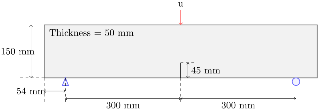
Figure 9: Dimensions and boundary conditions of the mode-I fracture test with a high strength concrete beam.

Table 1: Material constants used in the mode-I fracture test of the high-strength concrete beam.

Symbol	Values	Units
$E$	$33.89$	GPa
$f_{t}$	$3.39$	MPa
$G_{f}$	$116.15$	N/m

The uniform grid spacing is 2 mm, and the horizon is set to 6.03 mm. The stable time step is calculated as $4.64\times 10^{-7}$ seconds, and the local damping coefficient is set to $2.0\times 10^{7}$ kg/m${}^{3}\cdot$s. The characteristic dimension, L, is selected as the beam depth, which is 150 mm.

The local damage contour plots, shown in Figure 10, illustrate the numerically predicted cracks for both monotonic and cyclic loading cases. As seen in Figure 10, beams under both loading conditions fail due to straight crack propagation from the tip of the pre-notch to the loading zone at the top middle part of the beam, consistent with mode-I failure. The damage localizes in a narrow band, forming a well-defined crack path that propagates vertically from the notch tip toward the loading point. In addition, the similarity in crack patterns between the monotonic and cyclic loading cases indicates that the fundamental fracture mechanism remains unchanged regardless of the loading history.

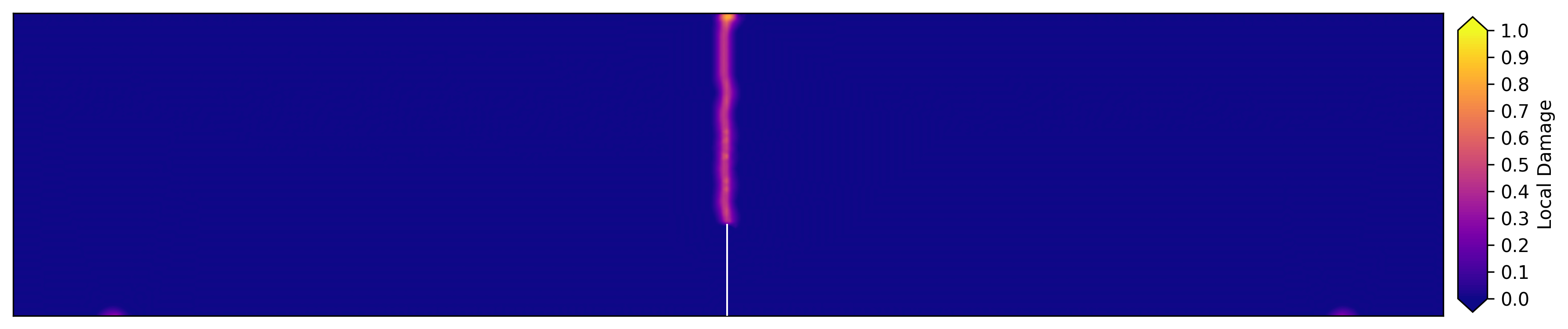
(a)

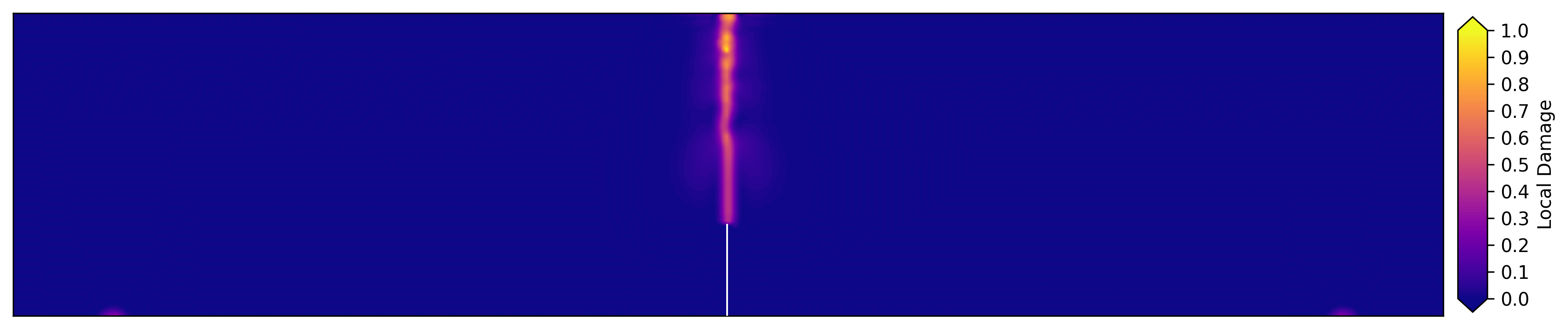
(b)

Figure 10: Local damage contour plots showing the crack trajectories obtained under (a) monolithic loading, and (b) cyclic loading.

The comparison of numerical and experimental load vs. Crack Mouth Opening Displacement (CMOD) curves is presented in Figure 11 for both monotonic and cyclic loading cases. In both cases, an excellent agreement is observed between the numerical and experimental results. For the monotonic loading case, provided in Figure 11(a), the numerical simulation accurately captures the initial linear elastic response, the peak load, and the general softening behavior. The peak load of approximately 3.3 kN closely matches the experimental value. For the cyclic loading case, presented in Figure 11(b), the numerical model successfully reproduces the characteristic hysteresis loops observed in the experiment. The loading paths of each cycle and the peak loads at various CMOD values align well with the experimental data. It is worth noting that the numerical curves return to the origin at the end of each unloading cycle, whereas the experimental curves do not due to accumulated plastic deformation. This occurs because the current model only considers fully elastic unloading and reloading. However, since our focus is primarily on brittle and quasi-brittle materials and failure mechanisms, plastic deformations are not as significant as in ductile failure. Therefore, this difference is considered acceptable for this study.

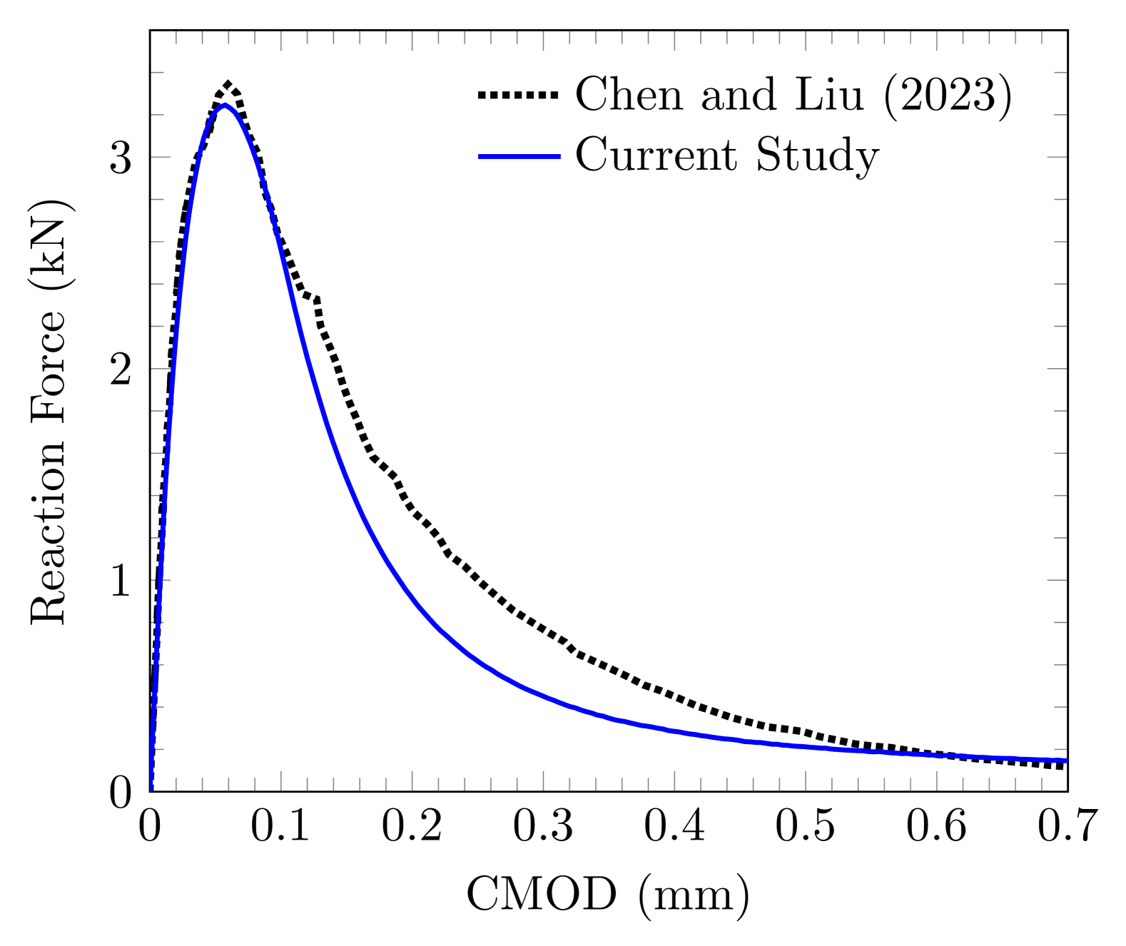
(a)

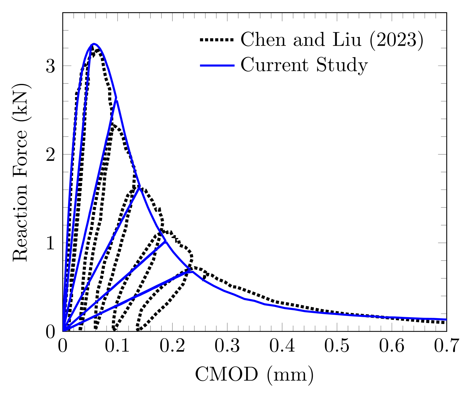
(b)

Figure 11: Comparison of experimental and numerical force vs CMOD curves for (a) monolithic, and (b) cyclic loading. Experimental data: black dotted Line; numerical results: blue solid line.

The results demonstrate that the proposed blended formulation can effectively model the mode-I fracture behavior of high-strength concrete under both monotonic and cyclic loading conditions. Although the current model does not account for permanent deformations during unloading cycles, it provides a reasonable approximation for the overall mechanical response of quasi-brittle materials like high-strength concrete.

8.2 Mixed-mode fracture tests on concrete beams under cyclic loading

Mixed-mode failure of concrete, where a combination of tensile and shear modes exists, is commonly observed in concrete structures. Meanwhile, as Jenq and Shah (1988) stated earlier, crack trajectories resulting from mixed-mode failure are far more complex than those occurring due to mode-I failure. Jenq and Shah (1988) studied crack initiation theories using linear elastic fracture mechanics (LEFM) and proposed a mixed-mode crack stability criterion. To verify their proposed model, they conducted a series of experiments, and we use their experimental findings to evaluate the performance of our numerical model. The dimensions and boundary conditions of the selected beams are presented in Figure 12. The compressive strength and Young’s modulus are provided in the reference study as 34.3 MPa and 32.8 GPa, respectively. However, the tensile strength and critical fracture energy release rate are not specified. Therefore, the values given in Table 2 are selected and kept constant for all tests conducted in this section.

In the reference study, the offset ratio, $\gamma$, is defined as the ratio of distance x (see Figure 12) to half the span length (half the distance between the two supports). Four sets of experiments were performed for each test, corresponding to $\gamma=0,\;1/6,\;1/3,\;\text{and }1/2$. It is important to note that the force vs. CMOD curves obtained from the study by Jenq and Shah (1988) are presented as ”typical force-CMOD” curves. Unfortunately, the study does not provide all four experimental curves for each test. Therefore, we cannot assess the variation in the force-displacement responses of the beams. In addition, the exact loading and unloading protocol is not provided in the experimental study; therefore, the applied displacements (please see the supplementary materials) are selected such that the unloading points match with the experimental ones as closely as possible. However, the final crack paths for each test are available in the reference study by Jenq and Shah (1988) and are used to compare the predicted crack trajectories with the experimental ones.

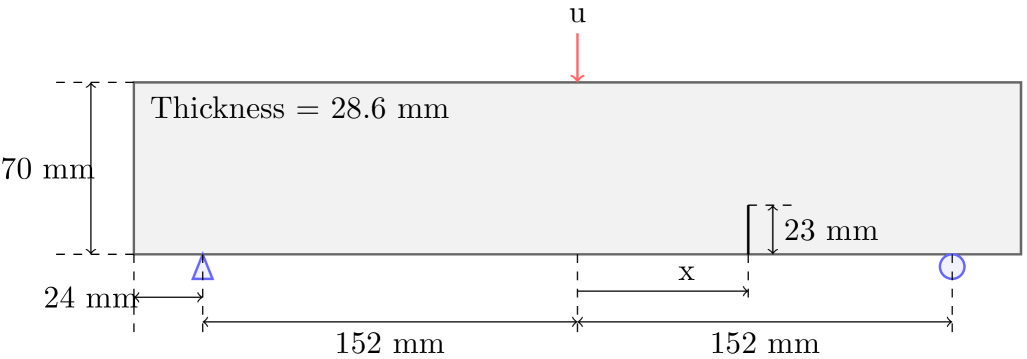
Figure 12: Dimensions and boundary conditions of the mixed-mode fracture tests on concrete beams.

Table 2: Material constants used in the mixed-mode fracture tests of the concrete beams.

Symbol	Values	Units
$E$	$32.8$	GPa
$f_{t}$*	$3.25$	MPa
$G_{f}$*	$115$	N/m

*Not provided in the experimental study by Jenq and Shah (1988).

In the numerical models, the uniform grid spacing is 1 mm and the horizon is selected as 3.015 mm. The local damping coefficient is used as $4.0\times 10^{7}$ kg/m${}^{3}\cdot$s, and the time step is selected as $2.36\times 10^{-7}$ seconds. The characteristic dimension, L, is chosen as the beam depth, which is 70 mm.

It is important to note that since the values for $f_{t}$ and $G_{f}$ are not provided in the reference study conducted by Jenq and Shah (1988), we calibrated these values by comparing the force vs CMOD curves for the mode-I test shown in Figure 13(a). However, these values remain unchanged for the remaining tests, i.e., no additional calibration was performed for the mixed-mode failure cases.

By comparing the typical force vs. CMOD response from the experimental study, we observe that the force-carrying capacity of the beams is underestimated for the mixed-mode tests, as shown in Figures 13(b) - 13(d).

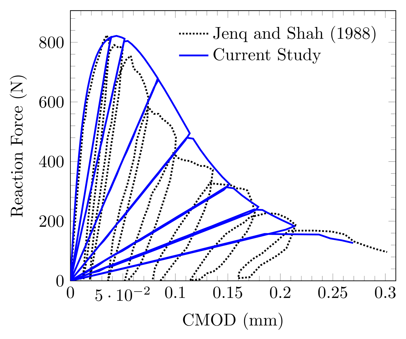
(a) x = 0 mm ($\gamma=0$)

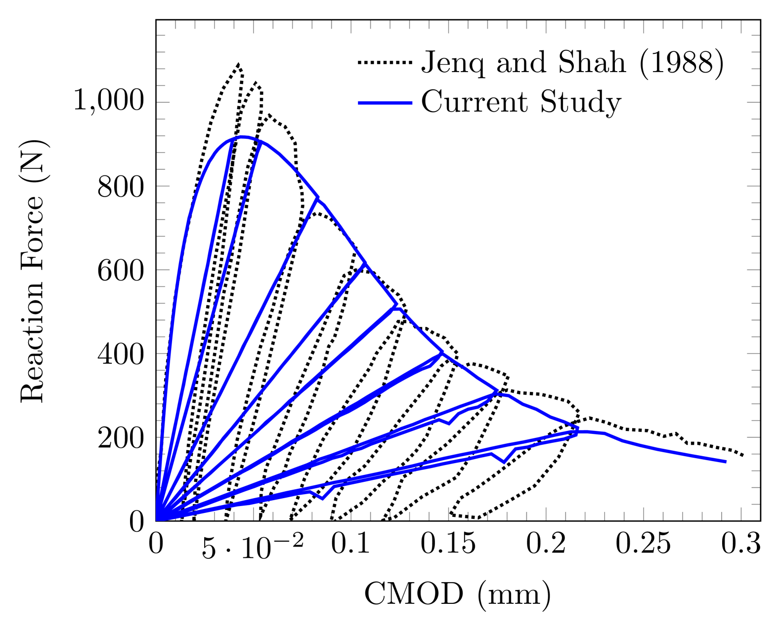
(b) x = 25 mm ($\gamma=1/6$)

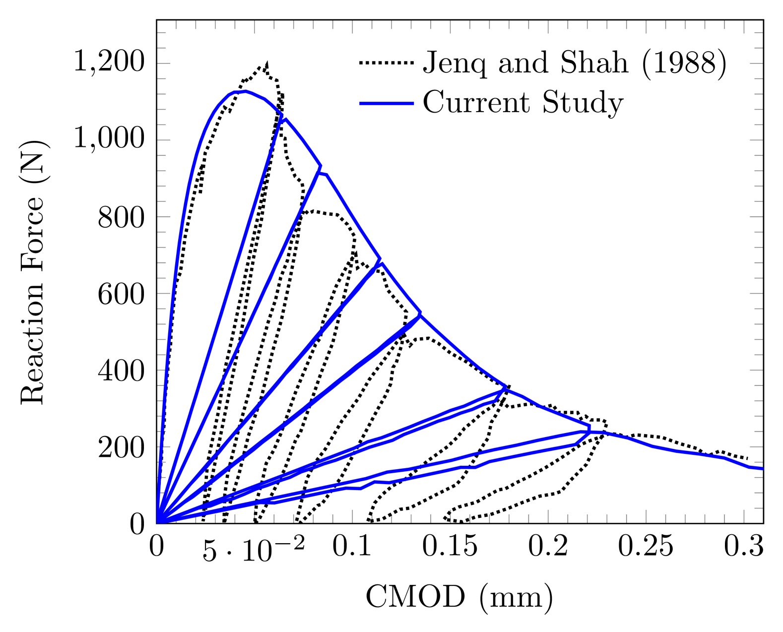
(c) x = 50 mm ($\gamma=1/3$)

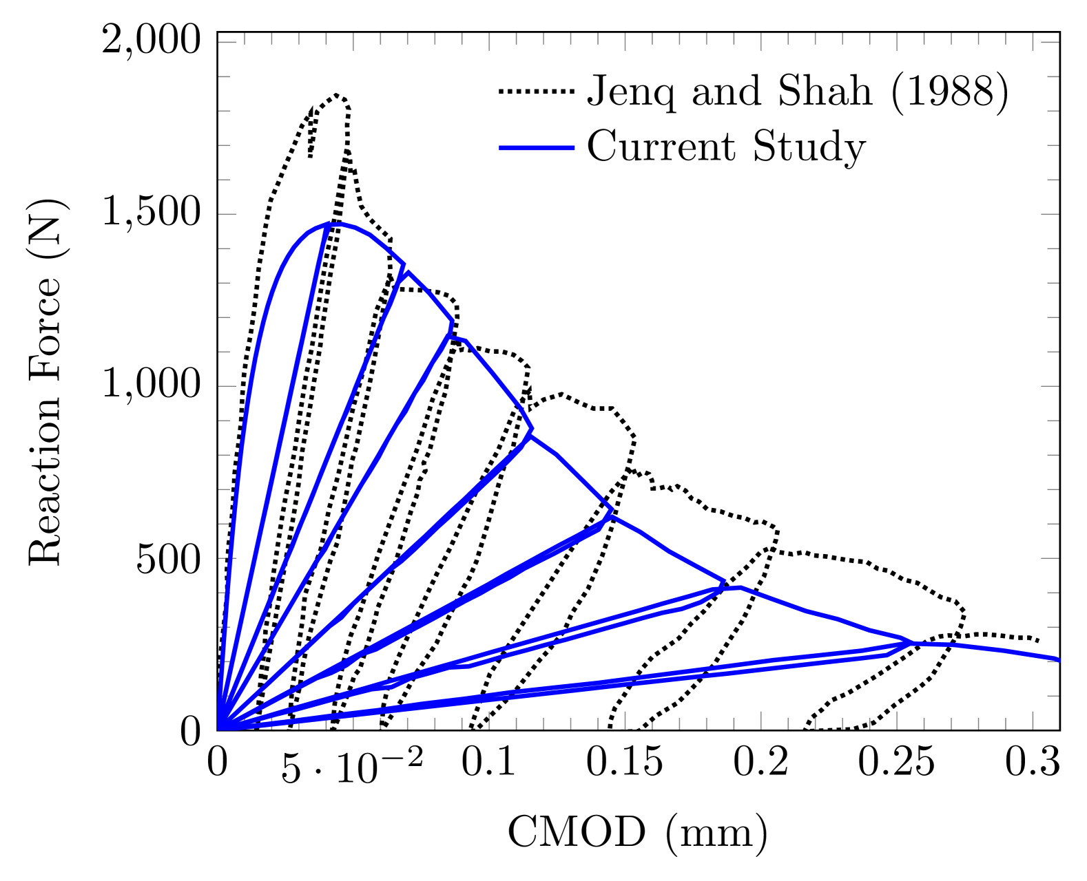
(d) x = 76 mm ($\gamma=1/2$)

Figure 13: Comparison of experimental and numerical force vs CMOD curves for the offset values: (a) x=0, (b) x= 25 mm, (c) x=50 mm, and (d) x=76 mm. Experimental data: black dotted Line; numerical results: blue solid lines.

The final crack paths obtained from the numerical simulations are compared with the experimental ones in Figure 14. Here, four experimental tests for each pre-notch location are shown as solid gray lines, while the blue solid lines represent the numerically predicted crack trajectories, drawn from the damage variable contour plots. In order to obtain crack trajectories from the numerical results, horizontal displacement contour plots are used. The horizontal displacement contour plots as well as the damage contour plots can be found in the supplementary materials of this study.

We believe Figure 14 highlights two important conclusions. Firstly, the crack paths obtained from the numerical simulations align well with the experimentally observed ones. Secondly, noticeable variations exist within the experimental results, even though the material properties and boundary conditions were intended to be the same. Concrete is a composite material where micro-cracks and voids are inevitable, even in undamaged specimens. In addition to the interaction between micro-cracks, the stiffness variations among its constituents (e.g., the mortar matrix and different sizes/types of aggregates) contribute to these discrepancies in the experimental results.

Furthermore, our numerical model treats concrete as a homogeneous material and does not account for micro-scale effects. Nevertheless, our numerical results exhibit strong agreement with the experimental findings, providing an accurate modeling approach for fracture simulations in quasi-brittle materials.

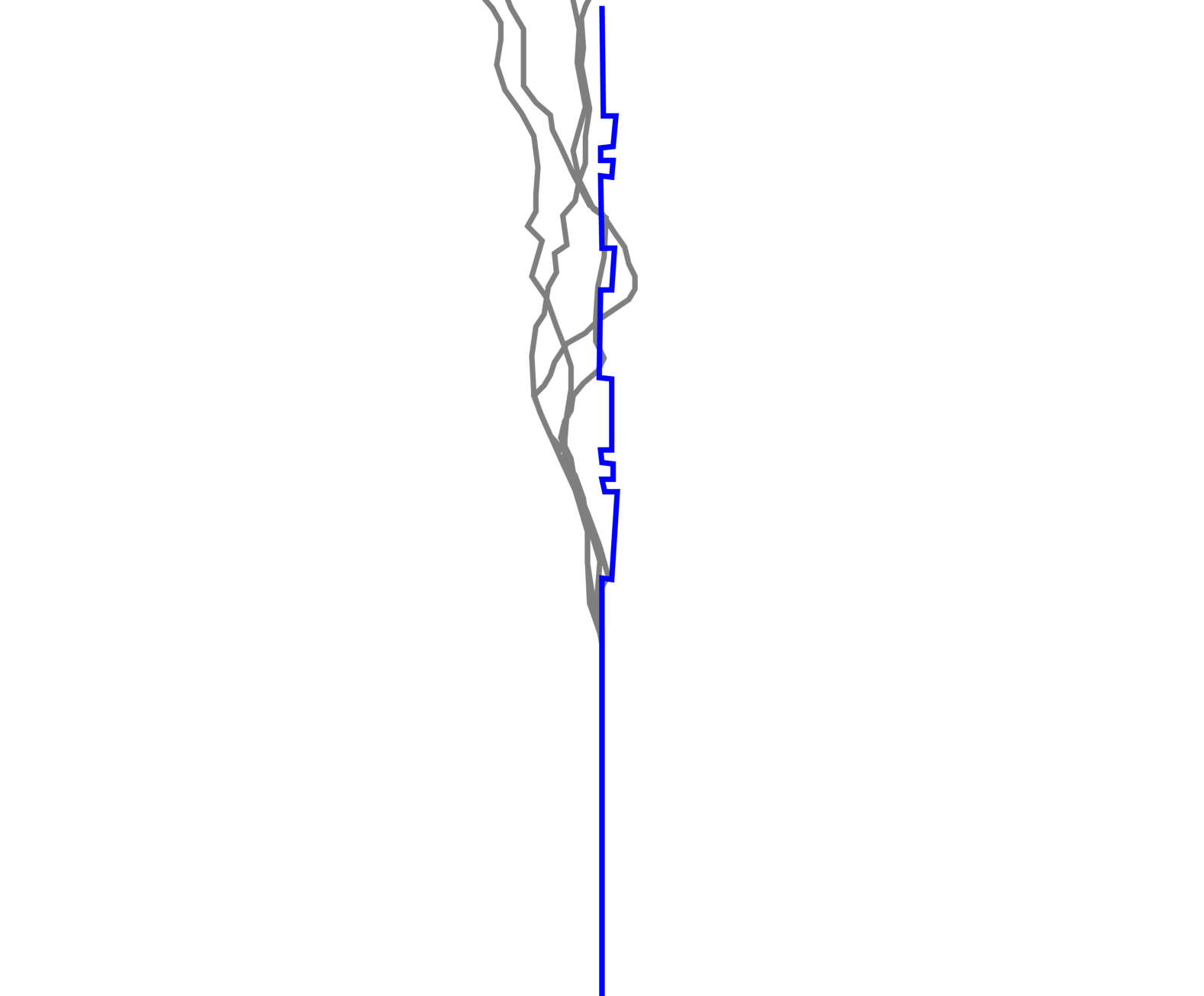
(a) x = 0 mm

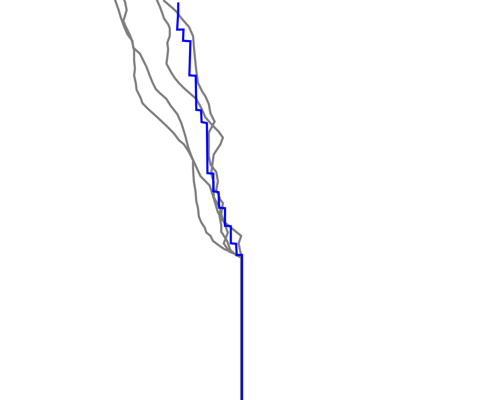
(b) x = 25 mm

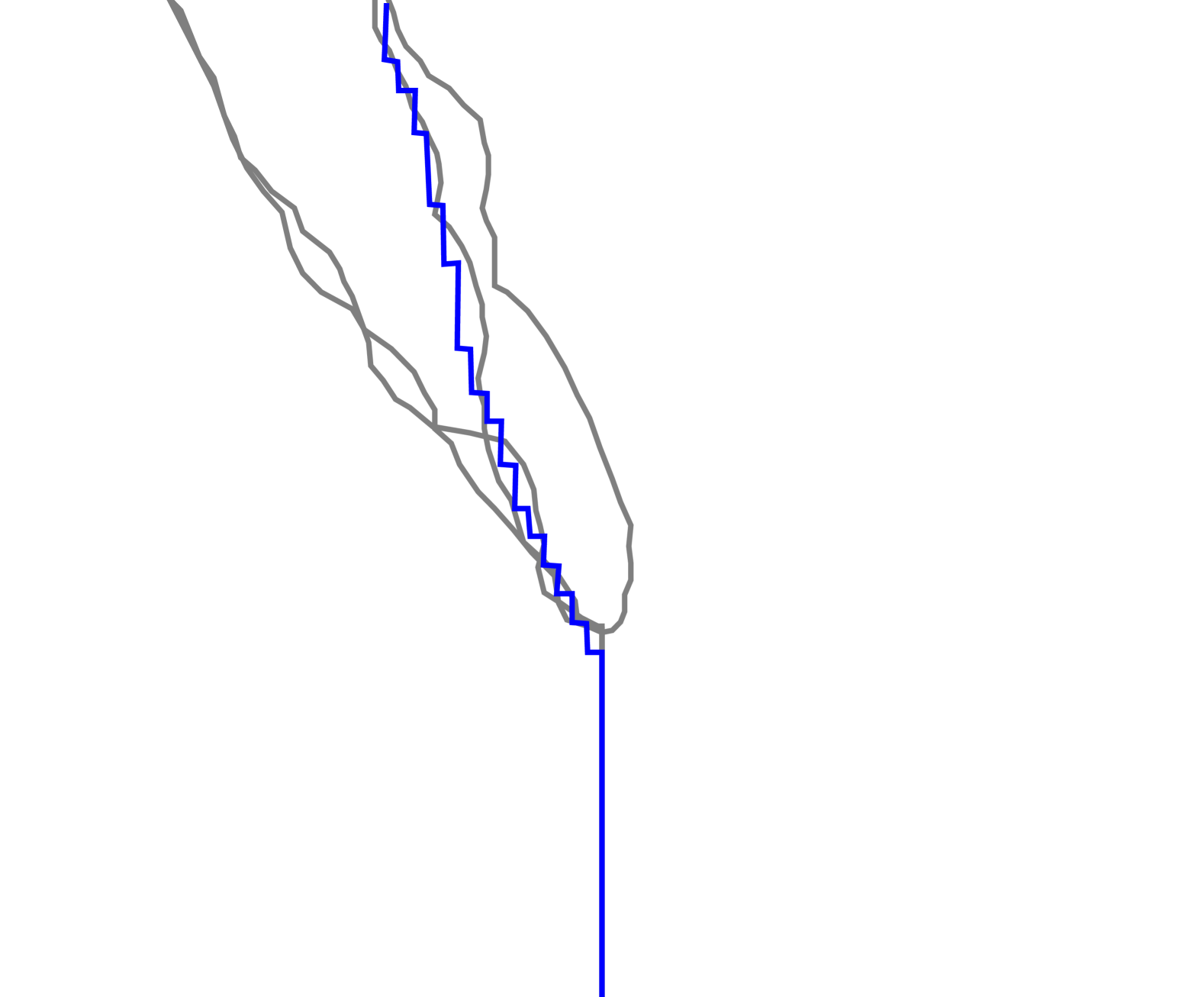
(c) x = 50 mm

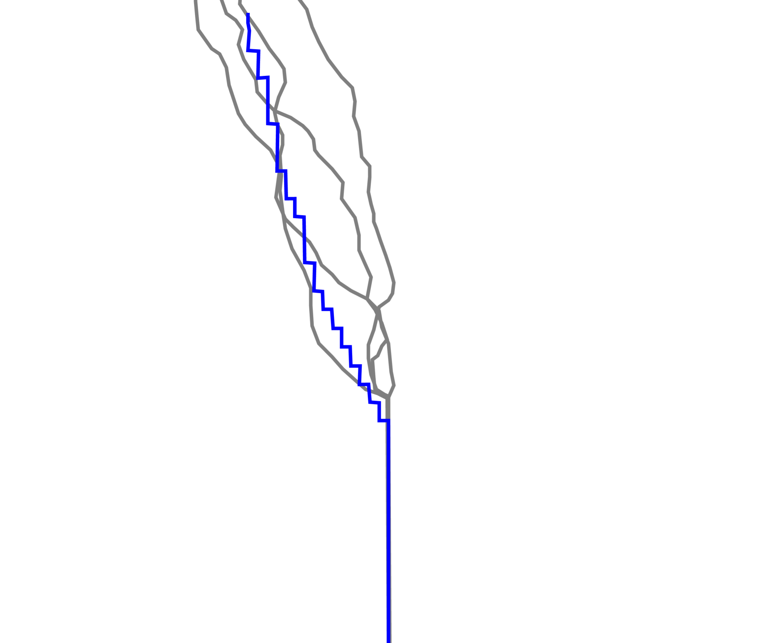
(d) x = 76 mm

Figure 14: Comparison of the crack trajectories for the offset distances (a) x=0, (b) x= 25 mm, (c) x=50 mm, and (d) x=76 mm. While gray solid lines represents the experimental crack paths borrowed from Jenq and Shah (1988), blue solid lines are obtained from the local damage plots.

8.3 Mixed-mode fracture of concrete L-shaped panel

As the third numerical example, we study the mixed-mode fracture test of an L-shaped concrete panel without a pre-notch. The experimental test was performed in a displacement-controlled manner by Winkler (2001). The dimensions and boundary conditions are presented in Figure 15.

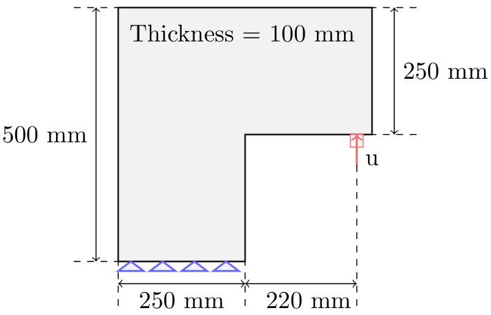
Figure 15: Dimensions and boundary conditions of the mixed mode fracture test with l-shaped concrete panel.

The L-shaped specimen has external dimensions of 500 mm $\times$ 500 mm with a thickness of 100 mm. The internal corner forms a 90^∘ angle with dimensions of 250 mm $\times$ 250 mm. The specimen geometry creates a stress concentration at the internal corner, which initiates a mixed-mode fracture.

Since the numerical model does not incorporate rotational degrees of freedom, the clamped boundary conditions are applied by constraining the displacements in both directions through a layer with a height equal to the horizon size, as shown in Figure 15. The vertical displacements are applied to a square region as a linearly increasing function, reaching a final value of 0.65 mm over 125 time steps. The stable time is calculated as $8.77\times 10^{-8}$ seconds and the local damping coefficient is set to $2.0\times 10^{7}$ kg/m${}^{3}\cdot$s. The uniform grid size is 2.5 mm and the horizon size is selected as 7.875 mm. The characteristic dimension, L, is selected as the length of the domain where the crack propagates, which is 250 mm.

The material properties listed in Table 3 are taken as it is given in the experimental work conducted by Winkler (2001) except the Young’s modulus. The Young’s modulus is selected as 18 GPa, which better represents the initial slope of the experimental force-displacement curves.

Table 3: Material constants used in the mixed-mode fracture test of the concrete panel.

Symbol	Values	Units
$E$*	$18$	GPa
$f_{t}$	$2.7$	MPa
$G_{f}$	$90.0$	N/m

*Different than the experimental values provided by Winkler (2001): E=25.85 GPa.

Figure 16 presents the comparison of the experimental and numerical load vs displacement curves for the mixed-mode fracture test of the concrete l-shaped panel. As can be seen from this figure, the load-carrying capacity as well as the softening behavior are predicted by the proposed model within an acceptable accuracy. The numerical model predicts a peak load of approximately 8 kN, which is slightly higher than the experimental average of around 7 kN. The initial elastic response up to approximately 0.15 mm displacement closely matches the experimental observations, confirming the appropriateness of the adjusted Young’s modulus. The post-peak softening behavior follows the general trend of the experimental data, though our model predicts a slightly more rapid decrease in load capacity between 0.3 mm and 0.45 mm displacement compared to the experimental range.

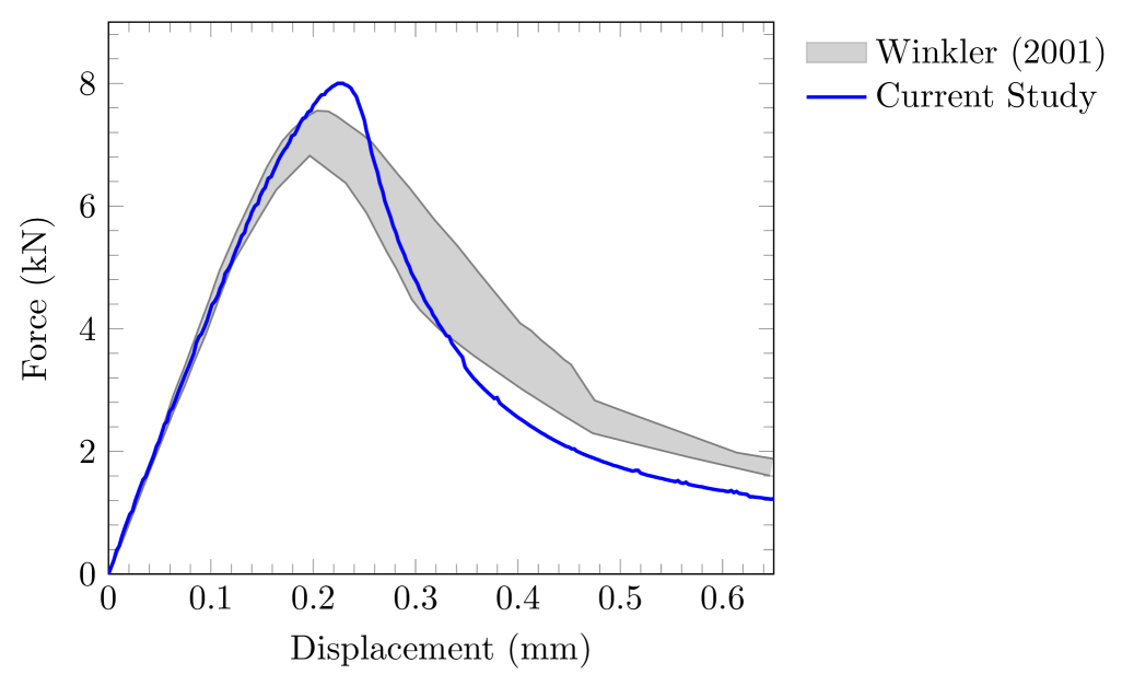
Figure 16: Comparison of experimental and numerical force vs displacement curves. Experiment: gray shaded region, numerical: solid blue line.

Figure 17(a) illustrates the local damage contour plot at the final displacement step. The damage localizes along a curved path starting from the inner corner of the L-shaped panel, which is the region of the highest stress concentration. The crack initiates in a mixed-mode fashion due to the combined tension and shear stresses at the inner corner, and it propagates toward the upper edge of the specimen.

Figure 17(b) provides a comparison between the numerically predicted crack trajectory and the experimental observations. The gray shaded region represents the experimental crack paths observed across multiple specimens, showing some natural variability in the experiments. The red solid line indicates our numerical prediction, which falls well within the experimental region. The crack path exhibits a characteristic curved trajectory that starts perpendicular to the maximum principal stress direction at the inner corner and gradually curves upward as it propagates.

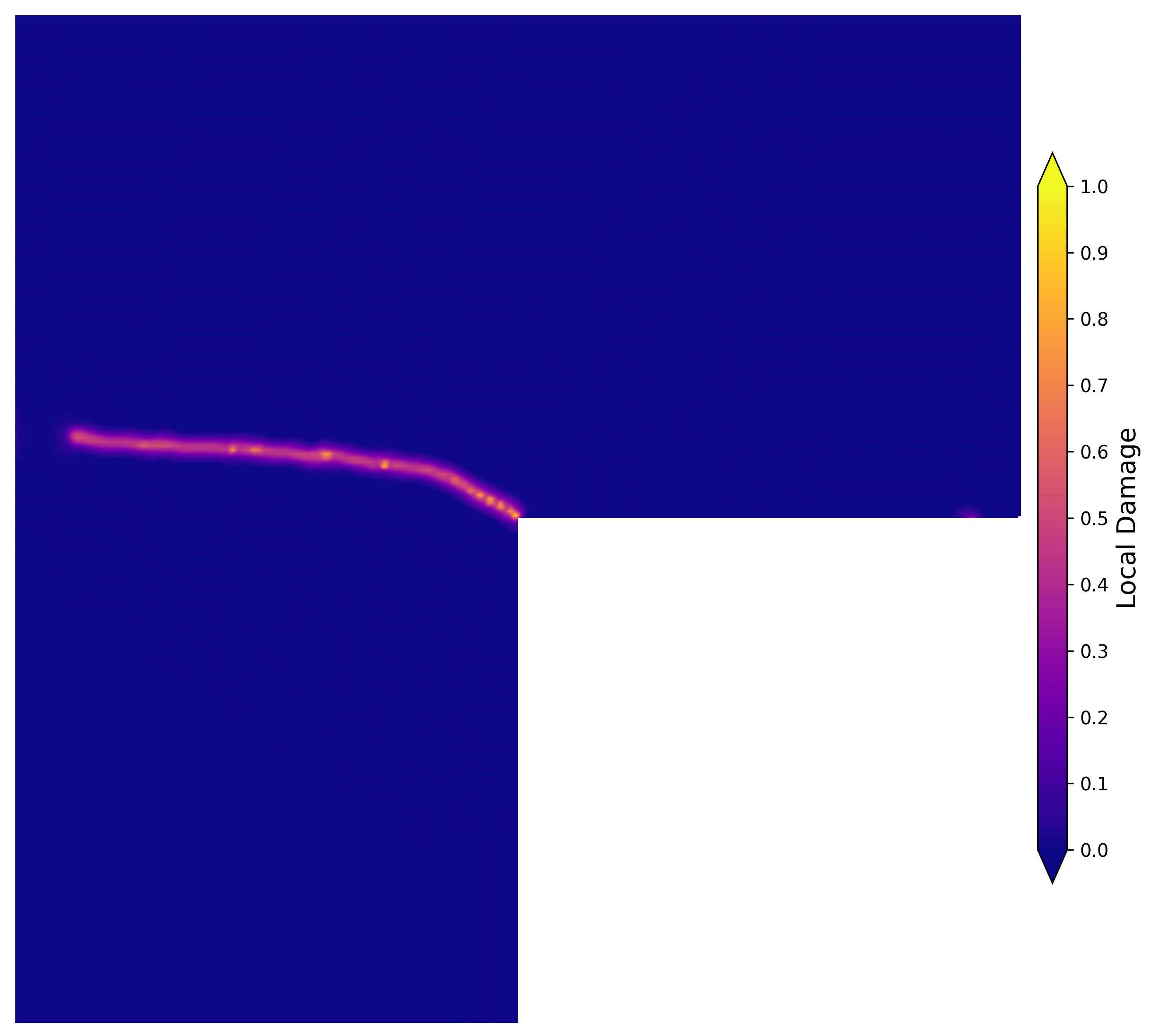
(a)

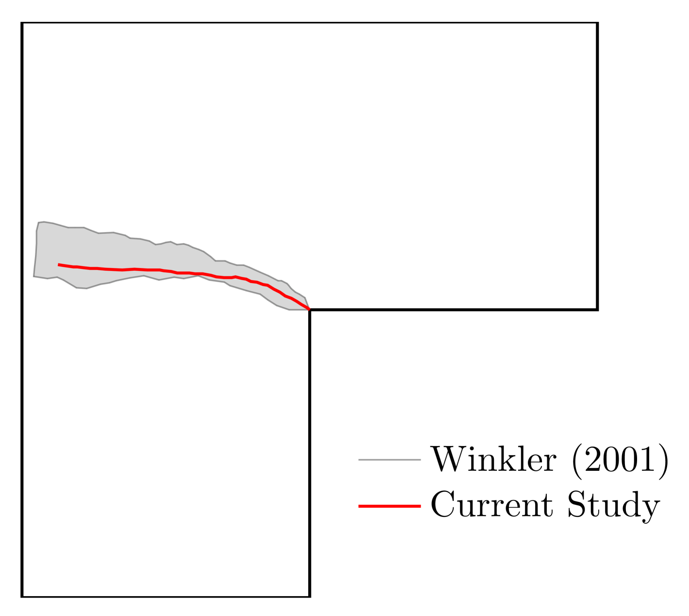
(b)

Figure 17: (a) Local damage contour plot and (b) comparison of the crack trajectories.

The agreement between the numerical and experimental crack trajectories demonstrates the capability of the proposed model to accurately capture the mixed-mode fracture behavior in concrete structures without the need for pre-defined crack paths or special interface elements.

8.4 Dynamic crack propagation in a glass plate

Dynamic crack propagation in brittle materials has been extensively studied (Freund (1990), Fineberg et al. (1992), Ravi-Chandar (2004), Zhou et al. (2005), Bobaru and Zhang (2015), Bleyer et al. (2017), Rakici and Kim (2023)) due to its importance in understanding failure mechanisms. In this section, we present numerical simulations of dynamic crack propagation in Duran 50 glass under suddenly applied tensile stresses.

The computational domain consists of a rectangular specimen with dimensions 100 mm $\times$ 40 mm containing a pre-notch of 50 mm length positioned at the mid-height of the left edge, as illustrated in Figure 18. The specimen is subjected to tensile stress, $\sigma$, applied uniformly along the top and bottom edges. Two different loading scenarios were investigated: a lower stress intensity case with $\sigma=$ 2 MPa and a higher stress intensity case with $\sigma=$ 12 MPa. The damage evolution and crack propagation characteristics were monitored throughout the simulation time frame. The material properties of Duran 50 glass, which are borrowed from Döll (1975), used in the simulations are summarized in Table 4.

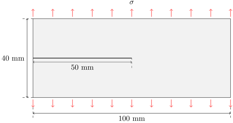
Figure 18: Dimensions and boundary conditions of the dynamic problem.

Table 4: Material constants for Duran 50 glass.

Symbol	Values	Units
$E$	$65$	GPa
$f_{t}$	$50$	MPa
$G_{f}$	$204$	N/m

A uniform mesh with a grid spacing of 0.4 mm is employed throughout the computational domain. The proposed blended formulation is implemented with a horizon parameter of 1.206 mm, defining the nonlocal interaction range. Since this numerical simulation addresses a transient problem, the local damping coefficient is set to zero to accurately capture the dynamic effects. To ensure the numerical stability of the explicit solver, a time step of 10 nanoseconds is utilized, satisfying the necessary CFL condition. These spatial and temporal parameters remain constant for both loading scenarios, enabling direct comparison between the low-stress (2 MPa) and high-stress (12 MPa) intensity cases. The characteristic dimension, L, is selected as the length of the domain where the crack propagates, which is 100 mm.

Figure 19 presents the damage variable contour plots for both loading conditions at the end of the simulation. For the lower stress case, where $\sigma=$ 2 MPa, the crack propagates in a straight path along the horizontal mid-plane of the specimen, as shown in Figure 19(a). This behavior is typical of mode-I fracture under moderate loading conditions where the crack follows the path of maximum energy release rate.

In contrast, the higher stress case, where $\sigma=$ 12 MPa, exhibits crack branching phenomena, as shown in Figure 19(b). Initially, the crack propagates horizontally, but at approximately 24.3 $\mu s$, it bifurcates into two distinct crack paths forming a Y-shaped pattern. This branching behavior is a well-documented phenomenon in dynamic fracture mechanics of brittle materials under high-intensity loading conditions, where the energy release rate exceeds a critical threshold that makes a single crack path energetically unfavorable.

Since there is no need for a crack tracking algorithm in the proposed model, a post-processing algorithm was used to determine the crack tip location and velocity to present these results. The crack region was determined using a damage threshold criterion which was selected as 0.38. Nodes with damage values exceeding this threshold limit were identified as a part of the crack region. Since the coordinates and the corresponding damage values were available as output of the solver, the crack tip was identified as the rightmost x-coordinate where damage exceeded the threshold. In order to detect the crack branching, the distribution of the y-coordinates at this rightmost position were analyzed to determine the distance exceeding 2.0 mm, which indicates a crack branching. The crack tip velocity was calculated using a linear regression approach with a window size of 12 data points in order to minimize the noise in the measurement. Hence, this regression provided the instantaneous velocity which will be then normalized with respect to the material’s Rayleigh wave speed, $c_{R}$.

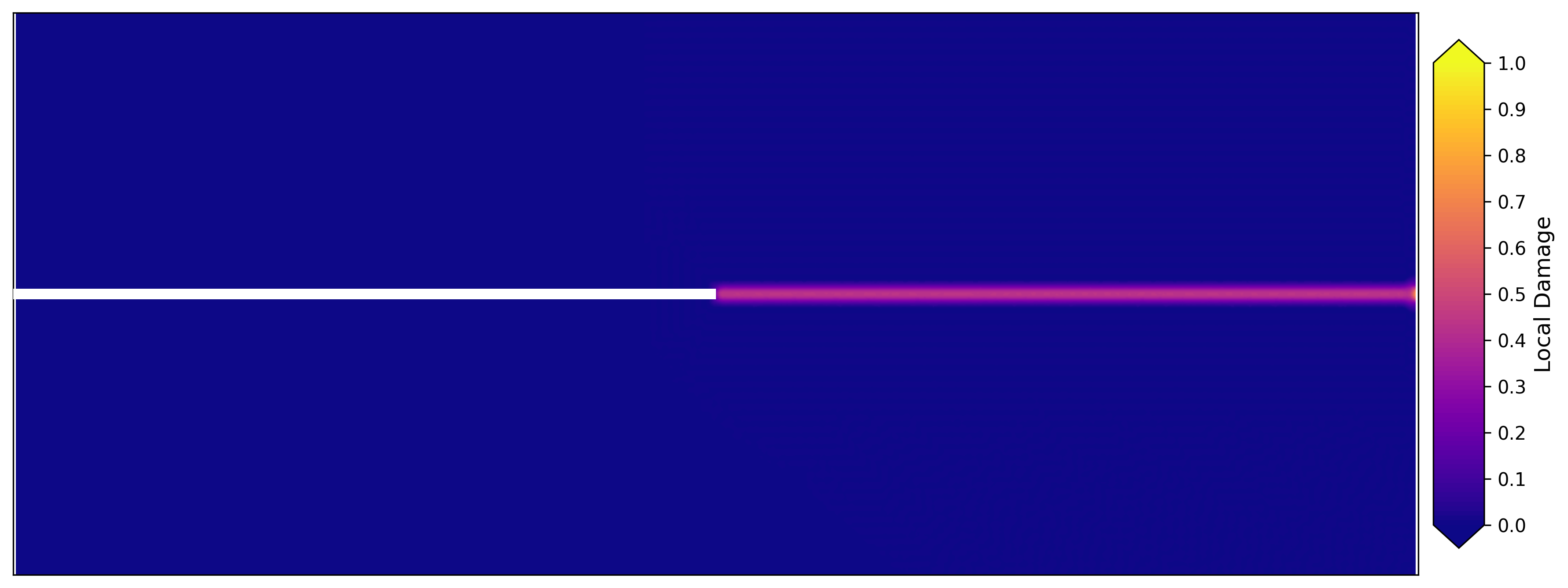
(a)

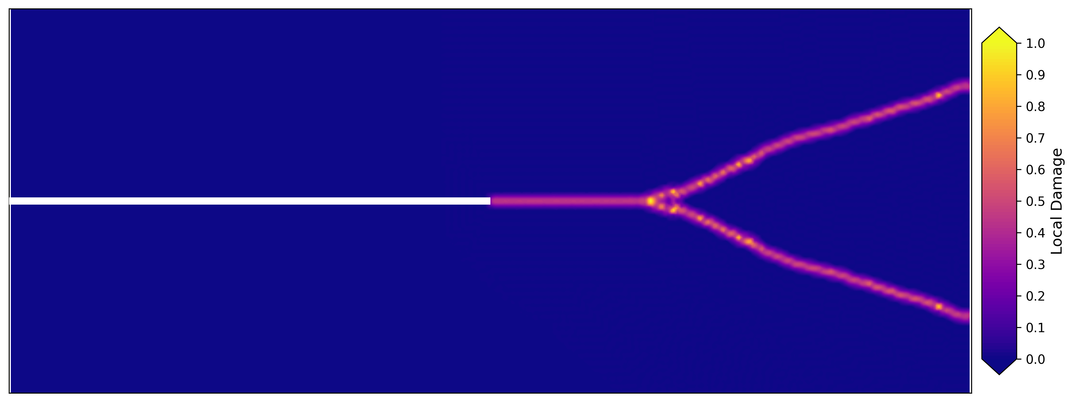
(b)

Figure 19: Damage variable contour plots for $\sigma=$ (a) 2 MPa, and (b) 12 MPa. White solid line represents the pre-notch.

Figure 20 presents the ratio of the crack tip speed to the Rayleigh wave speed, $c_{R}$ and the position of the crack tip with respect to time for the lower stress case ($\sigma=$ 2 MPa). As can be seen from Figure 20(a), the crack tip speed is well below $0.4c_{R}$ throughout the simulation. Figure 20(b) exhibits three different phases: initial acceleration, near-constant velocity, and deceleration phases. The initial acceleration phase occurs between 40-80 $\mu s$, where the crack tip speed reaches approximately $0.3c_{R}$. Then, the crack maintains a relatively stable speed in the near-constant velocity phase in 80-100 $\mu s$. After 100 $\mu s$, a deceleration phase follows, where the crack gradually slows down as it approaches the right boundary.

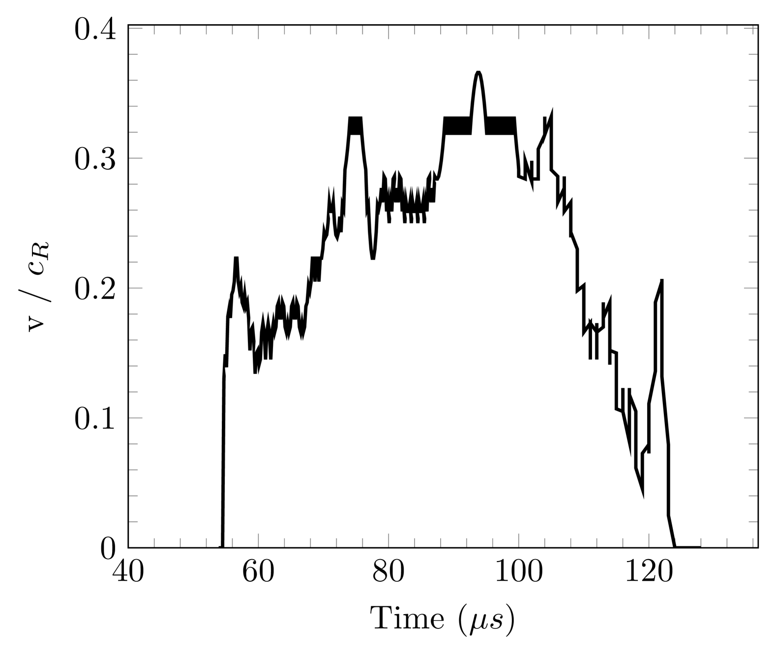
(a)

(b)

Figure 20: Dynamic crack propagation under $\sigma=$ 2 MPa, (a) crack tip speed to Rayleigh wave speed ratio, and (b) crack tip position with respect to time.

For the higher stress case, the crack tip speed to $c_{R}$ ratio is given in Figure 21(a), and the crack tip location with respect to time is plotted in Figure 21(b). Figure 21(a) shows that the crack tip velocity stays below $0.6c_{R}$, however, reaching values higher than in the previous case where the stress intensity is lower. In addition, the crack initially accelerates more rapidly, reaching higher velocities just below 0.6 times the Rayleigh wave speed. Between 10-25 $\mu s$ crack tip velocity shows greater fluctuations indicating unstable crack growth. After the crack branching at 24.3 $\mu s$, the fluctuations in the velocity profile of the crack tip are decreasing, which may indicate a more stable crack propagation than before the branching. For the higher stress case, the crack tip position with respect to time, presented in Figure 21(b), shows a nearly linear relationship, indicating a more constant average propagation speed compared to the lower stress case exhibited in Figure 20(b).

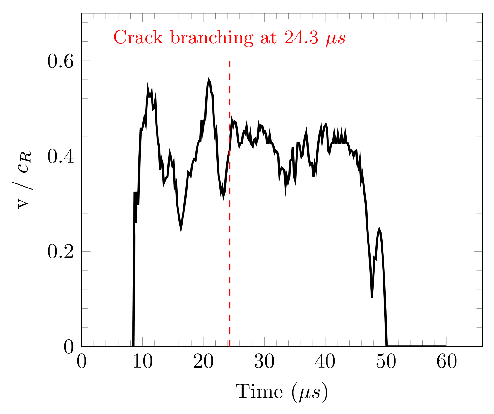
(a)

(b)

Figure 21: Dynamic crack propagation under $\sigma=$ 12 MPa, (a) crack tip speed to Rayleigh wave speed ratio, and (b) crack tip position with respect to time.

Therefore, it is shown that the crack propagation behavior in Duran 50 glass is highly dependent on the applied stress intensity. The transition from stable crack growth at $\sigma=$ 2 MPa to unstable crack branching at $\sigma=$ 12 MPa is consistent with experimental observations in brittle materials. In addition, the maximum crack velocity observed in our simulations remains below $0.6c_{R}$, which agrees with the theoretical limit proposed by Freund (1990), where crack velocities in brittle materials typically do not exceed 0.6-0.7 times the Rayleigh wave speed. This limitation is attributed to energy dissipation mechanisms and the increasing instability of the crack path at higher velocities.

8.5 Studying the size effect in concrete beams

Bažant and Planas (1998) defines the structural size-effect as the deviation of the actual load-carrying capacity of the structure, due to the change of its size, from the one predicted by any deterministic theory where the failure of the material is expressed in terms of stress and/or strain. However, classical failure theories such as plastic limit analysis or maximum allowable stress or strain criterion do not depend on the size of the specimen under consideration, which is problematic since experiments show a strong size-effect in the failure of brittle and quasi-brittle materials.

To study the size-effect, we choose to work on the mode-I failure tests for different sized beams made from the same concrete mix. The experiments were performed by Garc´ıa-Álvarez et al. (2012). The dimensions of the beams are summarized in Table 5 and the material properties of the concrete are given in Table 6.

Table 5: Dimensions of the beams tested for the mode-I failure test.

Specimen	Depth (mm)	Span (mm)	Thickness (mm)	Prenotch Length (mm)
Beam 1	80	200	50	20
Beam 2	160	400	50	40
Beam 3	320	800	50	80

Table 6: Material constants used in the mode-I fracture test of the concrete beams.

Symbol	Values	Units
$E$	$33.8$	GPa
$f_{t}$	$3.5$	MPa
$G_{f}$	$80.0$	N/m

Since the size-effect represents the dependence of the strength of the structure on its size, one first needs to define a measure of the strength of the structure and then compare the strength values obtained for different sizes with similar geometry of the specimen. The strength of the structure is conveniently characterized by the nominal stress at the maximum load. For this purpose, we calculate the ligament stress values at the ultimate load and use this value as the nominal strength of the beam. Since the beams are loaded under the three-point-bending set-up, the nominal strength of the beams can be calculated as

$$\sigma_{\text{lig}}=1.5\frac{F_{ult}\;s}{b\;h^{2}}$$ (8.2)

where $F_{ult}$ is the ultimate (maximum) load that the beam carries, $s$ is the length of the span, $b$ is the thickness of the beam, and $h$ is the length of the ligament (difference between the depth of the beam and the length of the pre-notch).

In the numerical simulations, the uniform grid spacing is 2 mm and the horizon is selected as 6.03 mm. The characteristic dimension, L, is chosen as the beam depth of the medium size beam, which is 160 mm. Here, our results are compared with the experimental findings of Garc´ıa-Álvarez et al. (2012) and the peridynamic bond based model presented by Hobbs et al. (2022). Once the maximum load carrying capacities are obtained from Figure 22 for each experimental and numerical tests, the strength values can be calculated using Eq. (8.2) and plotted with respect to beam size as shown in Figure 23. Hence, the relation between the size and strength of the structure obtained from the experimental findings can be clearly seen, and the performance of two different peridynamic models to capturing the size-effect can be discussed.

In this study, we implemented a simple bilinear model to capture the softening effect observed in the quasi-brittle materials. Whereas, Hobbs et al. (2022) use a constitutive relation where there is initial exponential decay with a linear tail. Both models use the elastic modulus and the tensile strength of the material given in Table 6. On the other hand, Hobbs et al. (2022) use an estimated value for the fracture energy of 125.2 N/m which is obtained from an equation given in a design code. Here, we stay with the value provided in the original experimental work conducted by Garc´ıa-Álvarez et al. (2012).

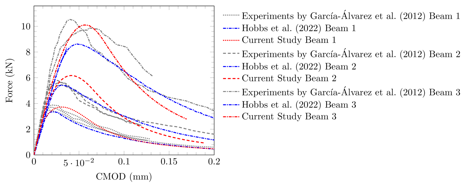
Figure 22: Comparison of the force vs CMOD curves for the mode-I fracture test.

Figure 22 presents the load-CMOD results for beam 1, beam 2, and beam 3 whose dimensions are given in Table 5. The experimental curves are plotted by gray, Hobbs et al. (2022)’s results by blue, and current results by red colored lines. The results of beams 1, 2, and 3 are plotted with dotted, dashed, and dash-dotted lines, respectively. As can be seen from Table 5, as beam 1 represents the smallest, beam 3 represents the largest among the three beams. The comparison of the peridynamic and blended models shows a subtle difference in the post-peak regime mainly because of the difference in the implemented constitutive models. In addition, the peak loads, or load-carrying capacities, show variation for the two numerical models, which may be a result of the selected fracture energy values as well as the constitutive models.

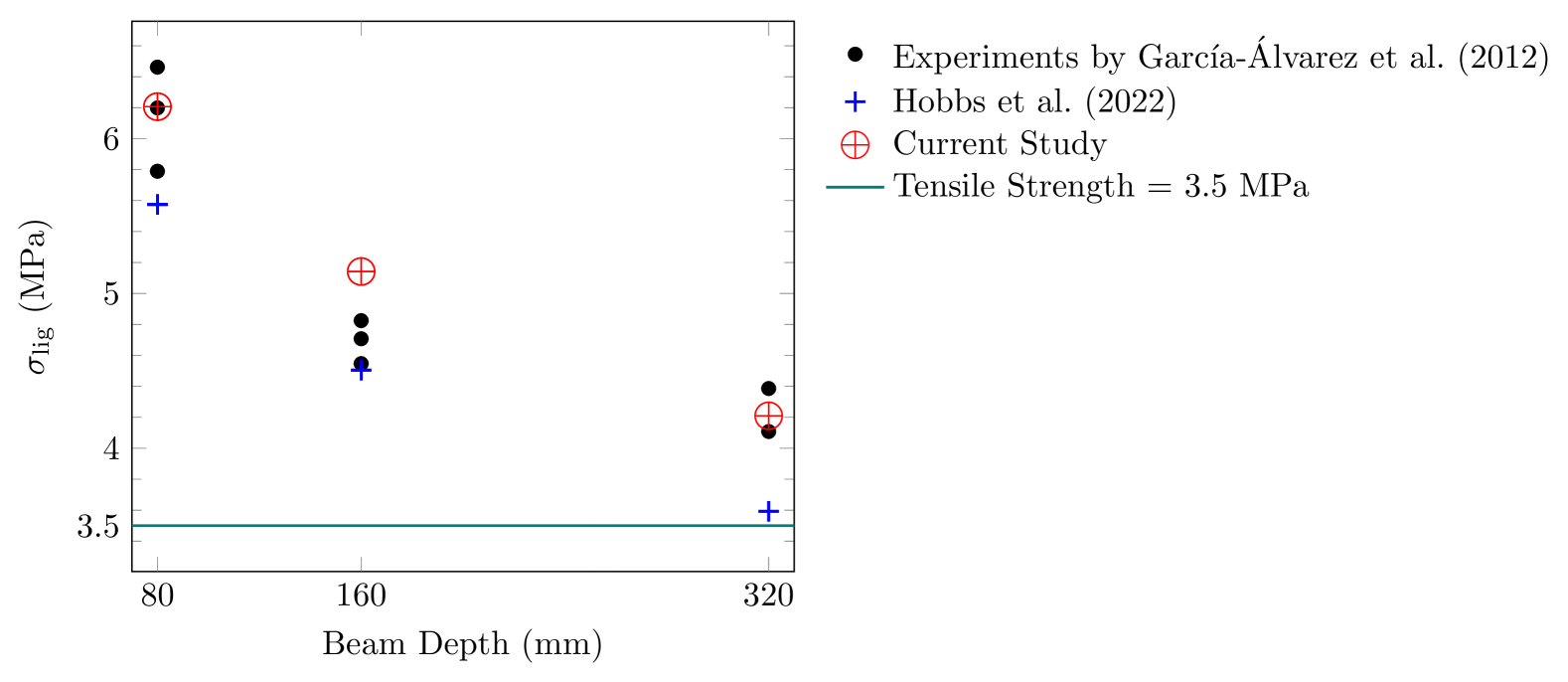
Figure 23: Nominal strength values with respect to beam depth.

The nominal strength values, corresponding to the ligament stress at the peak load and calculated using Eq. (8.2), are plotted with respect to the depth of the beam in Figure 23. While the tensile strength of the material is plotted by the teal solid line, the nominal strength values corresponding to each experimental test are shown with black-filled circles. As can be seen from the experimental values, there exists a strong dependence of the strength of the concrete beam on its size such that the average nominal strength values are obtained as 6.15 MPa, 4.7 MPa, and 4.25 MPa for the small, medium, and large beams, respectively. If the maximum allowable stress criterion is selected to be used as the ultimate tensile strength, the strength of beams 1 and 2 are significantly overestimated (43% and 26%, respectively). On the other hand, both blended and peridynamic bond based models exhibit a great performance capturing the size dependency on the strength values regardless of the differences in their constitutive models. It is important to note that none of the blended and peridynamic models employ an explicit rule to determine material strength based on sample size.

9 Conclusions

The blended model is formulated as a mathematically well-posed initial value boundary value problem for the displacement inside a quasi-brittle material. The solution is given by the displacement, damage field, and crack set history. The model inherently satisfies energy balance principles, with a positive energy dissipation rate that complies with the Clausius-Duhem inequality. These properties are not artificially imposed but emerge naturally from the material’s constitutive law and the evolution equation.

In the numerical examples, the simplest possible constitutive rule is intentionally chosen to minimize the number of material and numerical constants. By utilizing Young’s modulus, tensile strength, and fracture energy, the numerical constants can be determined, yielding both qualitative and quantitative results that align closely with the experimental data. The numerical simulations demonstrate excellent agreement with the experimental results for several benchmark problems, including mode-I fracture in concrete beams, mixed-mode fracture in notched specimens, fracture in L-shaped panels, and dynamic crack propagation. In particular, the same set of material constants and constitutive model successfully captures the size-effect phenomenon across three different beam sizes without incorporating any explicit rules for determining strength based on sample size. These results confirm the model’s ability to replicate real-world material behavior with minimal computational complexity.

10 Acknowledgment

This material is based upon work supported by the U. S. Army Research Laboratory and the U. S. Army Research Office under Contract/Grant Number W911NF-19-1-0245 and W911NF-24- 2-0184.

Data availability The code used to generate the results in this study is available at
https://github.com/SemsiCoskun/PDBlend.

References

- Aranson et al. (2000) Aranson, I., Kalatsky, V., Vinokur, V., 2000. Continuum field description of crack propagation. Physical review letters 85, 118. doi:https://doi.org/10.1103/PhysRevLett.85.118.
- Bažant and Planas (1998) Bažant, Z., Planas, J., 1998. Fracture and Size Effect in Concrete and Other Quazibrittle Materials. volume 1. CRC Press. doi:https://doi.org/10.1201/9780203756799.
- Bleyer et al. (2017) Bleyer, J., Roux-Langlois, C., Molinari, J.F., 2017. Dynamic crack propagation with a variational phase-field model: limiting speed, crack branching and velocity-toughening mechanisms. International Journal of Fracture 204, 79–100. doi:https://doi.org/10.1007/s10704-016-0163-1.
- Bobaru and Zhang (2015) Bobaru, F., Zhang, G., 2015. Why do cracks branch? a peridynamic investigation of dynamic brittle fracture. International Journal of Fracture 196, 59–98. doi:https://doi.org/10.1007/s10704-015-0056-8.
- Bourdin et al. (2000) Bourdin, B., Francfort, G.A., Marigo, J.J., 2000. Numerical experiments in revisited brittle fracture. Journal of the Mechanics and Physics of Solids 48, 797–826. doi:https://doi.org/10.1016/S0022-5096(99)00028-9.
- Bourdin et al. (2008) Bourdin, B., Francfort, G.A., Marigo, J.J., 2008. The variational approach to fracture. Journal of elasticity 91, 5–148. doi:https://doi.org/10.1007/s10659-007-9107-3.
- Chen and Liu (2023) Chen, H., Liu, D., 2023. Fracture process zone of high-strength concrete under monotonic and cyclic loading. Engineering Fracture Mechanics 277, 108973. doi:https://doi.org/10.1016/j.engfracmech.2022.108973.
- Döll (1975) Döll, W., 1975. Investigations of the crack branching energy. International Journal of Fracture 11, 184–186. doi:https://doi.org/10.1007/BF00034729.
- Du et al. (2015) Du, Q., Tao, Y., Tian, X., 2015. A peridynamic model if fracture mechanics with bond-breaking. J. Elasticity doi:https://doi.org/10.1007/s10659-017-9661-2.
- Falk et al. (2001) Falk, M.L., Needleman, A., Rice, J.R., 2001. A critical evaluation of cohesive zone models of dynamic fractur. Le Journal de Physique IV 11, Pr5–43. doi:https://doi.org/10.1051/jp4:2001506.
- Fineberg et al. (1992) Fineberg, J., Gross, S.P., Marder, M., Swinney, H.L., 1992. Instability in the propagation of fast cracks. Physical Review B 45, 5146. doi:https://doi.org/10.1103/PhysRevB.45.5146.
- Freund (1990) Freund, L.B., 1990. Dynamic fracture mechanics. Cambridge university press.
- Garc´ıa-Álvarez et al. (2012) García-Álvarez, V.O., Gettu, R., Carol, I., 2012. Analysis of mixed-mode fracture in concrete using interface elements and a cohesive crack model. Sadhana 37, 187–205. doi:https://doi.org/10.1007/s12046-012-0076-2.
- Hobbs et al. (2022) Hobbs, M., Dodwell, T., Hattori, G., Orr, J., 2022. An examination of the size effect in quasi-brittle materials using a bond-based peridynamic model. Engineering Structures 262, 114207. doi:https://doi.org/10.1016/j.engstruct.2022.114207.
- Jenq and Shah (1988) Jenq, Y., Shah, S., 1988. Mixed-mode fracture of concrete. International Journal of Fracture 38, 123–142. doi:https://doi.org/10.1007/BF00033002.
- Karma et al. (2001) Karma, A., Kessler, D.A., Levine, H., 2001. Phase-field model of mode iii dynamic fracture. Physical Review Letters 87, 045501. doi:https://doi.org/10.1103/PhysRevLett.87.045501.
- Lipton (2014) Lipton, R., 2014. Dynamic brittle fracture as a small horizon limit of peridynamics. Journal of Elasticity 117, 21–50. doi:https://doi.org/10.1007/s10659-013-9463-0.
- Lipton (2016) Lipton, R., 2016. Cohesive dynamics and brittle fracture. Journal of Elasticity 124, 143–191. doi:https://doi.org/10.1007/s10659-015-9564-z.
- Lipton and Bhattacharya (2025) Lipton, R.P., Bhattacharya, D., 2025. Energy balance and damage for dynamic fast crack growth from a nonlocal formulation. Journal of Elasticity 157, 1–32. doi:https://doi.org/10.1007/s10659-024-10098-1.
- Máirt´ın et al. (2014) Máirtín, É.Ó., Parry, G., Beltz, G.E., McGarry, J.P., 2014. Potential-based and non-potential-based cohesive zone formulations under mixed-mode separation and over-closure–part ii: Finite element applications. Journal of the Mechanics and Physics of Solids 63, 363–385. doi:https://doi.org/10.1016/j.jmps.2013.08.019.
- Miehe et al. (2010) Miehe, C., Welschinger, F., Hofacker, M., 2010. Thermodynamically consistent phase-field models of fracture: Variational principles and multi-field fe implementations. International journal for numerical methods in engineering 83, 1273–1311. doi:https://doi.org/10.1002/nme.2861.
- Niazi et al. (2021) Niazi, S., Chen, Z., Bobaru, F., 2021. Crack nucleation in brittle and quasi-brittle materials: A peridynamic analysis. Theoretical and Applied Fracture Mechanics 112, 102855. doi:https://doi.org/10.1016/j.tafmec.2020.102855.
- Ortiz and Pandolfi (1999) Ortiz, M., Pandolfi, A., 1999. Finite-deformation irreversible cohesive elements for three-dimensional crack-propagation analysis. International journal for numerical methods in engineering 44, 1267–1282. doi:https://doi.org/10.1002/(SICI)1097-0207(19990330)44:9<1267::AID-NME486>3.0.CO;2-7.
- Pandolfi and Ortiz (2012) Pandolfi, A., Ortiz, M., 2012. An eigenerosion approach to brittle fracture. International Journal for Numerical Methods in Engineering 92, 694–714. doi:https://doi.org/10.1002/nme.4352.
- Rakici and Kim (2023) Rakici, S., Kim, J., 2023. A discrete surface correction method for bond-based peridynamics. Engineering Analysis with Boundary Elements 151, 115–135. doi:https://doi.org/10.1016/j.enganabound.2023.02.041.
- Ravi-Chandar (2004) Ravi-Chandar, K., 2004. Dynamic fracture. Elsevier.
- Rohatgi (2024) Rohatgi, A., 2024. WebPlotDigitizer. URL: https://github.com/automeris-io/WebPlotDigitizer.
- Silling (2000) Silling, S., 2000. Reformulation of elasticity theory for discontinuities and long-range forces. Journal of the Mechanics and Physics of Solids 48, 175–209. doi:https://doi.org/10.1016/S0022-5096(99)00029-0.
- Silling and Askari (2005) Silling, S.A., Askari, E., 2005. A meshfree method based on the peridynamic model of solid mechanics. Computers & structures 83, 1526–1535. doi:https://doi.org/10.1016/j.compstruc.2004.11.026.
- Silling et al. (2007) Silling, S.A., Epton, M., Weckner, O., Xu, J., Askari, E., 2007. Peridynamic states and constitutive modeling. Journal of Elasticity 88, 151–184. doi:https://doi.org/10.1007/s10659-007-9125-1.
- Trageser and Seleson (2020) Trageser, J., Seleson, P., 2020. Bond-based peridynamics: A tale of two poisson’s ratios. Journal of Peridynamics and Nonlocal Modeling 2, 278–288. doi:https://doi.org/10.1007/s42102-019-00021-x.
- Underwood (1983) Underwood, P., 1983. Dynamic relaxation, in: Computational Methods in Mechanics, Vol 1: Computational methods for transient analysis. Elsevier Science Publishers B.V., pp. 245–265.
- Verhoosel and De Borst (2013) Verhoosel, C.V., De Borst, R., 2013. A phase-field model for cohesive fracture. International Journal for numerical methods in Engineering 96, 43–62. doi:https://doi.org/10.1002/nme.4553.
- Winkler (2001) Winkler, B.J., 2001. Traglastuntersuchungen von unbewehrten und bewehrten Betonstrukturen auf der Grundlage eines objektiven Werkstoffgesetzes für Beton. Innsbruck University Press.
- Wu (2017) Wu, J.Y., 2017. A unified phase-field theory for the mechanics of damage and quasi-brittle failure. Journal of the Mechanics and Physics of Solids 103, 72–99. doi:https://doi.org/10.1016/j.jmps.2017.03.015.
- Xu and Needleman (1994) Xu, X.P., Needleman, A., 1994. Numerical simulations of fast crack growth in brittle solids. Journal of the Mechanics and Physics of Solids 42, 1397–1434. doi:https://doi.org/10.1016/0022-5096(94)90003-5.
- Zaccariotto et al. (2015) Zaccariotto, M., Luongo, F., Galvanetto, U., et al., 2015. Examples of applications of the peridynamic theory to the solution of static equilibrium problems. The Aeronautical Journal 119, 677–700. doi:https://doi.org/10.1017/S0001924000010770.
- Zhou et al. (2005) Zhou, F., Molinari, J.F., Shioya, T., 2005. A rate-dependent cohesive model for simulating dynamic crack propagation in brittle materials. Engineering fracture mechanics 72, 1383–1410. doi:https://doi.org/10.1016/j.engfracmech.2004.10.011.