On the (Dis)connection Between Growth and Primitive Periodic Points
Abstract
In 1972, Cornalba and Shiffman showed that the number of zeros of an order zero holomorphic function in two or more variables can grow arbitrarily fast. We generalize this finding to the setting of complex dynamics, establishing that the number of isolated primitive periodic points of an order zero holomorphic function in two or more variables can grow arbitrarily fast as well. This answers a recent question posed by L. Buhovsky, I. Polterovich, L. Polterovich, E. Shelukhin and V. Stojisavljević.
1 Introduction
Bézout theorems seek to explore the relation between the growth of a holomorphic function and the size of its zeros set. The classical Bézout theorem states that the number of zeros of polynomials over variables is bounded by the product of their degrees. A natural question is whether this theorem extends to general holomorphic functions. Here, the notion of degree is replaced by the notion of growth rate, measured by the asymptotic behavior of its maximum modulus function,
Jensen’s formula gives a full description of this relation in complex dimension 1. Formally, assuming that , Jensen’s formula implies that for every there exists such that
In [2] Cornalba and Shifmann showed this phenomenon does not extend to higher dimensions. They constructed a holomorphic function satisfying ,
whose zeros grow arbitrarily fast. Here, and everywhere else in the paper, means that there exists a constant for which .
In a recent paper, [1], L. Buhovsky, I. Polterovich, L. Polterovich, E. Shelukhin and V. Stojisavljević proposed a new way to obtain a transcendental analog to Bézout theorem, replacing the traditional zero count with the coarse zero count. Roughly speaking, the coarse count of zeros of a holomorphic function in is the number of connected components on which it is small, that contain a zero. They proved that this coarse count can be bounded in terms of the maximum modulus function, thus establishing an analog to Bézout theorem in the setup of coarse count.
This version of Bézout theorem can be imported into the world of complex dynamics. It implies that the coarse count of -periodic points of holomorphic functions is also bounded by a function of their growth rate. Moreover, the Cornalba-Shifmann example (shifted by the identity map) shows that the honest count of fixed points does not obey such a bound. In [1] they asked whether the construction carried out by Cornalba-Shifmann can be generalized to construct an order zero holomorphic function with arbitrarily many primitive periodic points of higher periods.
Definition 1.1
Let be a holomorphic function.
-
•
We say is -primitive periodic point for (or -PPP for short) if whenever , but .
-
•
Denote by the number of -PPP lying in a ball of radius centered at the origin, namely
Question 1.2 ([1, Question 1.12])
Does there exist a transcendental entire map, , of order 0 (i.e., the modulus grows slower than for every ) for which grows arbitrarily fast in and ?
For a fixed period, , a simple modification of the Cornalba–Shiffman example produces a holomorphic function, , of order zero for which grows arbitrarily fast in ; see Example 3.4 below. However, producing a holomorphic function with many primitive periodic points of varying prescribed periods is more complicated. Our main result states that this is indeed possible.
Theorem 1.3
For every sequence of periods, , and for every rate, , there exists a holomorphic function satisfying
The constant in is independent of the sequences.
Unlike the example by Cornalba and Shiffman, the holomorphic functions constructed in Theorem 1.3 are not completely explicit. In particular, it is not clear how to estimate or even bound from above or below their coarse zero count.
The main idea of the proof is to utilize the simple example constructed in Example 3.4 with different fixed periods, and then use a ‘dispatcher’ function to choose between different periods. The main tool in the construction is a theorem of Hörmander (see Theorem 3.3 below) which guarantees the existence of solutions to non-homogeneous -equations with certain integral bounds. This theorem allows one to construct entire functions with distinct behaviours in different regions. The use of Hörmander’s theorem requires an underlying subharmonic function which is large in the area between distinct regions, but very negative where we want a good approximation. Section 2 contains the construction of subharmonic functions that will be used in the application of Hörmander’s theorem in Section 3. In Section 3 we construct the required holomorphic functions and prove Theorem 1.3.
Acknowledgements
We thank Lev Buhovsky and Leonid Polterovich for useful discussions.
A.G. is grateful for the support of the Golda Meir fellowship.
S.T. was partially supported by a grant from the Institute for Advanced Study School of Mathematics, the Schmidt Futures program, a research grant from the Center for New Scientists at the Weizmann Institute of Science, and Alon fellowship.
2 Preliminary Results on Subharmonic functions
We commence the discussion with the following lemma whose role is to modify a given subharmonic function assigning to prescribed points.
Lemma 2.1 (The Puncture Lemma)
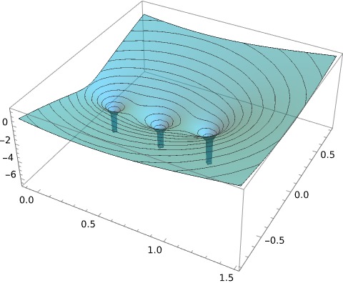
Let be a continuous subharmonic function and, for or , let be a sequence of pairwise disjoint disks, . Assume that for every , . Then there exists a subharmonic function satisfying
-
1.
whenever .
-
2.
For every , and
where is some uniform constant.
See Figure 1 for an illustration of the image of the subharmonic function .
While the proof can be found in [4, Section 3.1], where and the function is any function, we include it here for the reader’s convenience.
Proof.
Define the function
where (and therefore ), the constants will be chosen momentarily, and is Poisson integral of a function defined by
Note that is continuous, since the Poisson integral of any continuous function agrees with it on . We need to choose the constants such that sub-harmonicity is preserved. We will use the following claim:
Claim 2.2 ([3, p.24])
Let be a domain, and let be a domain, so that is an orientable smooth curve. Every function which is continuous on and subharmonic on , is subharmonic on if on it satisfies
where is the outer normal to along and is the outer normal to along .
We will use this claim with , and . In this case, we need to show that along
and the latter is known. To calculate we will use Poisson-Jenssen’s formula (see e.g. [7, Theorem 4.5.1]), which, in this case, boils down to:
where
Here, and throughout the rest of the paper, denotes Lebegue’s measure in . Using the above, we see that is subharmonic if for every :
using the fact that vanishes on (since there). Then if and only if
Since the collection is uniformly integrable, we may change the order of the integral and the derivative to obtain that
Note that is some uniform constant, which does not depend on the function or the collection . A direct computation shows that we may choose to be positive (this follows from the fact that the radial derivative of the Green function is everywhere non-negative and does not vanish identically). Setting guarantees that is subharmonic.
Finally, for every
∎
3 The proof
In this section we prove Theorem 1.3. Extending upon Example 3.4 below, we need a function that will coordinate between different periods. In Section 3.1, we construct a holomorphic function that assumes prescribed values along the sequence and whose role is to accommodate for different periods. This part uses the results on subharmonic functions and a theorem of Hörmander. In Section 3.2, we modify the construction by Cornalba-Shiffman, [2], to construct a holomorphic function of two variables with the required number of -PPP in every ball , and the required growth rate, thus proving Theorem 1.3.
3.1 Constructing the “dispatcher” functions
Lemma 3.1
There exists so that for every (finite or infinite) subset and every , there exists an entire function satisfying that
-
(i)
.
-
(ii)
.
Remark 3.2
We stress that is independent of and .
Proof.
As mentioned in the introduction, we use Hörmander’s Theorem (Theorem 3.3 below) to construct the “dispatcher” function. A crucial first step is the construction of an appropriate subharmonic function.
3.1.1 Step 1: Constructing an appropriate subharmonic function.
Denote by
where will be chose momentarily. Note that is subharmonic as a local maximum of subharmonic functions (along the maximum is and along the maximum is ). In addition, is a radial subharmonic function and for every
Define the collection of pairwise disjoint disks, for and , and note that .
3.1.2 Step 2: The model map and the holomorphic approximation.
Let and consider any (finite or infinite) subset . We define the model map
Let be a smooth map satisfying
-
1.
whenever .
-
2.
whenever .
-
3.
There exists a uniform constant such that
For a construction of such a function, see e.g. [5, Proposition 2.5].
In order to find a holomorphic map approximating the model map along the sequence of points while also providing growth bounds, we use Hörmander’s theorem:
Theorem 3.3
[Hörmander, [6, Theorem 4.2.1]] Let be a subharmonic function. Then, for every locally integrable function there is a solution of the equation such that:
| (2) |
provided that the integral in the right hand side is finite.
We define the function , which is supported in . Note that on the support of . To apply Hörmander’s theorem, we bound the following integral:
| (3) |
since , while if , the model map satisfies . It is important to note that is a numerical number which does NOT depend on or on the set .
We apply Hörmander’s theorem with the map and the subharmonic function , constructed in Step 1, to obtain a function satisfying and estimate (2), and define
It is not hard to see that is an entire function, as a solution to the equation.
3.1.3 Step 3: Bounding the error.
We will show that for every the function, , constructed above, agrees with the model map, , at .
Fix and note that for every , the function satisfies . Using Cauchy’s integral formula for the function , which on is both holomorphic and coincides with , we obtain that up to a uniform constant,
where the second inequality follows from Cauchy-Schwartz inequality. Using inequality (2) from Hormander’s Theorem, the above integral can be bounded by the integral of , which we estimated in (3.1.2). Combining these bounds with (3.1.1), we obtain
We conclude that , i.e., property (ii) holds.
3.1.4 Step 4: Bounding the growth.
To see that property (i) holds, we use a similar calculation noting that , since if , then and if then .
This time, we apply Cauchy’s integral formula to rather than , as is not necessarily holomorphic in these disks. We obtain
where we used the fact that . Overall, we see that
concluding the proof of Lemma 3.1. ∎
3.2 Modifying Cornalba-Shiffman’s construction
Before constructing an entire function with many primitive periodic points of different periods, let us explain a simple way to construct an entire function with many p-primitive periodic points for a single period, . Roughly speaking, the construction takes (a symmetrized version of) the Cornalba-Shiffman’s example and adds to it a standard rotation by , formally defined by , which rotates the plane by counter clockwise. Zeros of Cornalba-Shiffman’s construction then become -primitive periodic points.
Example 3.4
Fix . Note that while is a -periodic function, its periodic points are not isolated. Let be any entire function of order zero satisfying that in every ball of radius , has isolated zeros that are symmetric under the rotation :
Here, and everywhere else, is the composition of with itself times. One example of such function is a symmetrized version of the function constructed by Cornalba and Shiffman, which we explicitly synthesize in Lemma 3.6. However, any function with isolated symmetric zeroes as above will do. Then
is a holomorphic function of order zero satisfying that in every ball of radius it has points which are -PPP.
We would like to modify this construction, to construct functions with primitive periodic points of varying periods. For this we will use the dispatcher function constructed in the previous subsection. Our main goal for this section is to complete the proof of Theorem 1.3, which states that for every sequence of periods, , and for every rate, , there exists a holomorphic function satisfying
Remark 3.5
To simplify our notation we will assume our sequences start from . As the sequences are arbitrary, this does not limit the generality of the result.
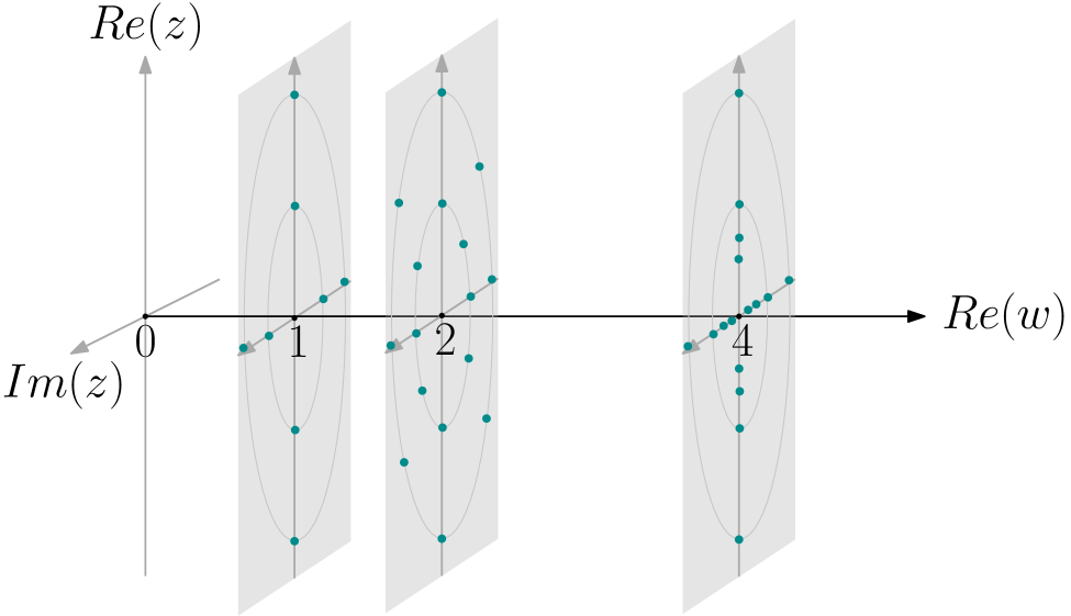
We start by constructing a “symmetrized” version of the Cornalba–Shiffman function, whose zero set is depicted in Figure 2.
Lemma 3.6
Given a sequence of periods, , and a rate, , there exists a holomorphic function of order zero satisfying
-
•
The set of isolated zeros of contains the set
-
•
and satisfies
-
•
, and , i.e., does not depend on .
-
•
There exists a uniform constant (independent of the sequences ) such that
Proof.
Similarly to Carnalba-Shiffman’s original construction, let
and for every consider the following polynomial of degree :
where , are the zeros of .
Define the function
where the sequence will be chosen throughout the proof so that satisfies the assertions of the lemma.
Derivatives and isolation of zeros: Starting with the requirement on the derivatives, it is clear that does not depend on . In addition, the derivative of with respect to is non-vanishing on since and
The estimate of the derivative of with respect to requires a computation of the derivatives of , using the symmetry of the set :
Let us related the derivatives at and . Shifting the product by we see that if we fix , the product over is taken over the entire set (shifted by ). On the other hand, if the product that was taken over the set shifted is the product taken over the set , which is the derivative at . We see that
implying that
Growth bound: To conclude the proof, we will show that the sequence can be chosen so that for some uniform constant .
We first bound the growth of the functions independently of . Fix , and let be so such that . Then,
The same computation shows that as well, which concludes the growth bound for .
Next we bound the growth of . The degree of the polynomial is , and it is bounded by
For every consider with . For simplicity of the arguments below, we assume that the sequence is strictly increasing. Note that this can be achieved by increasing , which does not change the statement of the lemma, as is the number of -PPP, increasing it will generate more points than required. Define . Then, since ,
| (4) |
We shall bound each sum separately.
To bound the first summand in (3.2), note that we may assume without loss of generality that (this happens whenever the sequence grows fast enough) and that . Then
where in the first inequality we used our choice of , and in the second, the fact that for , .
Combining the two estimates together, we see that
and thus the desired bound holds for as well, concluding our proof. ∎
We will use the lemma above to conclude the construction of a holomorphic map on with prescribed PPP’s for any sequences of periods and any rate.
Proof of Theorem 1.3.
In light of remark 3.5, for every we let be a dispatcher function created by the Dispatcher Lemma, Lemma 3.1, with , a singleton, and the constant . Recall that is a holomorphic function satisfying
We define the function
where is the modification of Cornalba-Shiffman’s construction constructed in Lemma 3.6 above.
We need to show that has at least isolated -PPP in every ball and that it satisfies the correct growth rate. As in Lemma 3.6, we define the sets
Observation 1: and every point in is a -PPP.
Indeed, note that
implying that
In particular, for every we have
concluding the proof of observation 1.
Observation 2: The points in are isolated -PPP.
Indeed, recall that for every ,
In addition, following Observation 1, , implying that for every we have
We write
Fix , we let , then as well and as ,
If is degenerate at , then
However, on one hand, by Lemma 3.6. On the other hand, following the same lemma, if we denote by
then for every ,
We conclude that
implying that
To estimate the latter, note that if , then as the both are polynomials of degree with the same roots (of unity) and leading coefficient 1. We derive from that,
and therefore
as . We conclude that is non-degenerate on , and the points in are isolated -PPP.
In fact, the same calculation shows that for every the point is isolated -PPP as well.
Observation 3: Growth bound- .
References
- [1] Lev Buhovsky, Iosif Polterovich, Leonid Polterovich, Egor Shelukhin, and Vukašin Stojisavljević. Persistent transcendental Bézout theorems. Forum of Mathematics, Sigma, (12), 2024.
- [2] Maurizio Cornalba and Bernard Shiffman. A counterexample to the “transcendental Bézout problem”. Annals of Mathematics, 96(2):402–406, 1972.
- [3] Vasiliki Evdoridou, Adi Glücksam, and Leticia Pardo-Simón. Unbounded fast escaping wandering domains. Advances in Mathematics, 417:108914, 2023.
- [4] Adi Glücksam. Harmonic measure of the outer boundary of colander sets. Studia Mathematica, 263:59–87, 2022.
- [5] Adi Glücksam and Leticia Pardo-Simón. An approximate solution to Erdös’ maximum modulus points problem. Journal of Mathematical Analysis and Applications, 531(1):127768, 2024.
- [6] Lars Hörmander. Notions of convexity. Springer Science & Business Media, 2007.
- [7] Thomas Ransford. Potential theory in the complex plane. Number 28. Cambridge university press, 1995.
A.G.: Einstein Institute of Mathematics, Edmond J. Safra Campus, The Hebrew University of Jerusalem, Givat Ram. Jerusalem, 9190401, Israel
https://orcid.org/0000-0002-6957-9431
adi.glucksam@mail.huji.ac.il
S.T.: Department of Mathematics, Weizmann Institute of Science 234 Herzl St. PO Box 26. Rehovot ,7610001, Israel
https://orcid.org/0000-0001-6389-6922
tanny.shira@gmail.com