Exploiting $\nu$-dependence of projected energy correlators in HICs

Abstract

We extend the recently derived factorization formula for energy-energy correlators to study the analytic structure of general $\nu$-point projected energy correlators in heavy ion collisions. The $\nu$-point projected energy correlators (or, $\nu$-correlators) are an analytically continued family of the integer $N$-point projected energy correlators, which probe correlations between $N$ final-state particles. By tracking the largest separation ($\chi$) between the $N$ particles, in vacuum, their structure is closely related to the DGLAP splitting functions and exhibits a classical scaling behavior $\sim 1/\chi$ which is modified by resummation through the anomalous dimensions. We show that, in a thermal medium, the $\nu$-correlators display non-trivial angular scaling already at the leading order in perturbation theory. We find that for non-integer values, particularly $\nu<1$, medium-induced jet function is enhanced compared to $\nu>1$. This is particularly manifested in the ratios of $\nu$-correlators with respect to the two-point energy correlator which encode an intrinsic angular information for $\nu<1$ when compared to large $\nu$ values. Moreover, for small-$\nu$ values, the $\nu$-correlators appear to saturate at $\nu=0.01$. We further confirm our leading-order numerical computations against simulated events from JEWEL for the parton level production cross-section. Finally, we qualitatively discuss the effect of BFKL resummation for various values of $\nu$.

[a]organization=Nikhef Theory Group, addressline=Science Park 105, city=Amsterdam, postcode=1098 XG, country=The Netherlands

[b]organization=Department of Physics, addressline=University of South Dakota, city=Vermillion, postcode=57069, state=SD, country=USA

1 Introduction

Jets are collimated sprays of hadrons generated through the evolution of an energetic quark/gluon (color charge parton) produced in a hard scattering event in particle collisions [1]. The evolution of this energetic parton spans through several energy scales, ranging from large perturbative to small non-perturbative, thereby encoding the dynamics of its branching history. In heavy-ion collisions (HICs), the color charge parton in the jet undergoes further interactions with the constituents of the quark gluon plasma (QGP). These interactions manifest themselves in form of medium-induced splittings or branchings contributing to in-medium evolution of the jet [2, 3, 4, 5, 6, 7, 8]. While the initial state hard scatterings producing the jet are expected to take place at a perturbative scale, the subsequent evolution at lower energy scales gets modified through the interactions with the medium [9, 10, 11]. As a result, the final jet observed in HICs retains signatures of the various stages of the medium, see Refs. [12, 13, 14, 15, 16, 17, 18] and references therein.

The interaction between a fast-moving color charge parton with the medium constituents occurs primarily through scattering processes, which can also trigger medium-induced radiation [19]. One such mechanism contributing to the in-medium evolution of jets is the Landau-Pomeranchuk-Migdal (LPM) effect, which is a coherent effect of multiple scattering centers in the medium [20, 21], see Ref. [22] for recent updates. As a result, the effective transverse momentum transfer by the medium is characterized by $\hat{q}$, which is the transverse momentum squared per unit length. Since a jet consists of multiple fast-moving color charge partons, these partons can interfere among themselves, forming interference patterns which leads to color coherence dynamics characterized by a coherence angle $\theta_{c}$. This implies that if the two prongs of the jet are separated by an angle $\theta>\theta_{c}$, they can act as independent sources of medium-induced radiation. Conversely, if $\theta<\theta_{c}$, medium-induced radiation is coherently sourced by the total color charge of the jet. Recently, in Ref.[10], it was pointed out that this scale may lead to new logarithmic structures that may give rise to non-trivial evolution of the jet in the medium. Over the past two decades, numerous theoretical and phenomenological efforts have been directed at formulating an understanding of jet-medium interactions in the presence of QGP medium [23, 24, 25, 26, 27, 16, 28, 29, 30, 31, 32, 33, 34, 35, 36, 37, 38, 39, 40, 41, 42, 43, 44, 45, 46].

In the context of HICs, the two primary considerations for understanding medium modifications on jets are (a) what are the best observables to quantify medium-induced evolution from the vacuum evolution, and (b) can we develop a theoretical framework that can be systematically improved along with providing controlled theoretical uncertainities? With respect to the first question, energy correlators have recently emerged as promising observables to quantify medium-induced jet dynamics, as they provide a direct connection to the fundamental field-theoretic energy flow observables. Various attempts have been made to understand the structure of the simplest case of the two-point energy correlator in the medium [47, 48, 49, 50, 51, 52, 53, 54]. While two-point correlations provide the simplest access to the transverse scales, higher-point correlations hold the potential for understanding the rich dynamics inherent to many-body QCD interactions. Recently, a few efforts have also been made to explore the structure of these higher-point energy correlators, see Refs [55, 56, 57]. Secondly, with regard to a systematic theoretical framework, in a series of papers in Refs. [34, 35, 38, 58, 45, 46], the authors initiated the first steps towards the development of such a systematic framework together with allowing for a dynamic treatment of the medium partons. Utilizing such an effective approach, the authors of Ref. [52] established the structure of the factorization theorem, in the collinear limit, for the computation of the two-point correlator in the medium [59, 60, 61, 62].

In this Letter, we further extend the factorization formula for the two-point correlator derived in Ref. [52], to understand the general structure of $\nu$ point projected energy correlators ($\nu$-correlators) in the medium. The $\nu$-correlators can be defined as an analytic continuation of the projected (integer) $N$-point correlators [63], which is a simple generalization of the two-point correlator that studies the correlations between $N$-final state particles by looking at the largest separation between them. In particular, these $N$-point projected correlators are analytically continuable in $N$, which we will denote as PE$\nu$C. This analytic continuation places all $\nu$-correlators into a single analytic family of observables. $\nu$-correlators are of particular significance due to their potential to probe the anomalous dimensions of the system, providing an access to the leading-twist collinear dynamics in jets. In particular, the $\nu$-correlators are formally defined as

$${\rm PE}\nu{\rm C}(\chi)\equiv\frac{{\rm d}\sigma^{[\nu]}}{{\rm d}\chi}=\sum_{M}\int{\rm d}\sigma_{X}\bigg{[}\sum_{1\leq a_{1}\leq M}{\cal W}_{1}^{[\nu]}(a_{1})\,\delta(\chi)\,+$$

$$\hskip 8.0pt\sum_{1\leq a_{1}<a_{2}\leq M}{\cal W}_{2}^{[\nu]}(a_{1},a_{2})\,\delta(\chi-\Delta R_{a_{1},a_{2}})\,+\dots+$$

$$\!\!\sum_{1\leq a_{1}<..<a_{M}=M}\hskip-20.0pt{\cal W}_{M}^{[\nu]}(a_{1},..,a_{M})\,\delta(\chi\!-\!{\rm max}\{\Delta R_{a_{1},a_{2}},..,\Delta R_{a_{M-1,M}}\})\bigg{]},$$ (1)

where ${\rm d}\sigma_{X}$ represents the production cross-section to produce the final state $X$ and $\Delta R_{ij}=\Delta\eta_{ij}^{2}+\Delta\phi_{ij}^{2}$ are the relative distance between particles $i$ and $j$ in the rapidity-azimuth plane. The weights ${\cal W}_{1,2,\dots}$ appearing in the above equation account for correlations between subsets of particles in the jet, with ${\cal W}_{1}^{[\nu]}$ representing all 1-particle correlations, ${\cal W}_{2}^{[\nu]}$ representing all 2-particle correlations, and so on. Here $M$ denotes the total number of particles in the jet.

PE$\nu$C’s provide several interesting avenues for studying the structure of QCD interactions using jets. First, in the vacuum, the distribution of PE$\nu$C’s is well governed by the moments of the time-like splitting kernels. Second, the $\nu\to 0$ limit further provides an access to study small-$x$ physics with jets. For the leading order splitting of a quark to a quark and gluon ($q\to q+g$), the vacuum distribution in the finite $\chi$ region exhibits a simple classical scaling as $\sim 1/\chi$ which is the same for all $\nu$-correlators. In particular [63],

$${\rm PE}\nu{\rm C}(\chi)=-\frac{2^{3-\nu}\alpha_{s}(\mu)\,C_{F}}{\pi}\frac{1}{\chi}\bigg{(}\frac{3(\nu-1)}{(\nu+1)}-4(\gamma_{E}+\psi^{(0)}(\nu))\bigg{)}\,.$$ (2)

Note that the fixed order distribution has a divergence as $\nu\to 0$ in the term proportional to $\delta(\chi)$ which we have not shown in the above equation, see Ref. [63] for the complete form. Resummation modifies this classical scaling and introduces an anomalous scaling behavior that depends on the value of $\nu$ as ${\rm d}\sigma^{[\nu]}/{\rm d}\chi\propto 1/\chi^{1-\gamma(\nu+1)}$, where $\gamma(\nu+1)$ is the anomalous scaling dimension related to the QCD splitting functions, specifically the $\nu$-th moment of the splitting function $P(x)$.

In the presence of a QGP medium where the jet parton undergoes further interactions with the thermal constituents, it is worth exploring the modification of this scaling dimension as a function of $\nu$. Similar to vacuum, one hopes to gain more insight on the structure of the anomalous dimensions and corresponding evolution of the jet and the medium through the use of $\nu$-correlators.

In this work, we restrict to the case of leading order jet function for the medium. At this order, we take the hard function ${\cal H}\equiv\{{\cal H}_{q},{\cal H}_{g}\}$ as $\delta(1-x)\choose 0$, therefore the results we obtain for the medium-induced jet function can directly be interpreted as the PE$\nu$C distributions that we are interested in.

This Letter is organized as follows: In Sec. 2, we provide details of the factorization formula for the $\nu$-correlators in the medium. In Sec. 3, we present the detailed computation of the medium-induced jet function at the leading order. Here we provide complete analytical structure by considering different phase-space regions for the transverse momentum exchanges with the medium as well as different hierarchies. In Sec. 4, we present the numerical results and also validate the results from our analytic set-up against the in-medium simulated events using JEWEL. Finally, we conclude in Sec. 5.

2 Factorization

2.1 Set up

In this section, we briefly review the relevant modes and factorization formula derived in Ref. [52]. To begin, we represent a four-vector in light cone variables as $p^{\mu}=(p^{-},p^{+},{\boldsymbol{p}})$ and assume that the jet moves in the positive z direction, i.e., $p^{-}\gg{\boldsymbol{p}}\gg p^{+}$. To facilitate factorization, we first define the momentum scaling for the collinear jet parton as $p^{\mu}_{n}\sim Q(1,\lambda^{2},\lambda)$ with $\lambda\sim\sqrt{\chi}$ being the power-counting parameter of the effective theory, and $Q\sim\mathcal{O}(p_{T})$ is the hard scale. Next, we define momentum scaling for soft medium partons as $p^{\mu}_{s}\sim(Q_{{\rm med}},Q_{{\rm med}},Q_{{\rm med}})$, where $Q_{{\rm med}}$ is an intrinsic medium scale. While the exact value of $Q_{{\rm med}}$ depends on single and multiple scattering scenarios (See Ref. [46]), we restrict ourselves in the single scattering limit and assume $Q_{{\rm med}}\sim$ (2-3) GeV. The interaction between the collinear jet parton and the soft partons of the medium is mediated by the exchange of off-shell Glauber gluons $\sim Q(\lambda,\lambda^{2},\lambda)$. For later convenience, we also introduce another momentum scaling of jet partons, namely collinear-soft modes $\sim Q\lambda(1,\lambda^{2},\lambda)$, which contribute to the measurement. For more details, see Refs.[52, 45, 46].

2.2 Factorization

We begin with the total density matrix, which includes both the medium and jet density matrices, and express its time evolution as

$$\rho(t)=e^{-iHt}\rho(0)e^{iHt},$$ (3)

where $H=H_{0}+C(Q)l^{\mu}j_{\mu}$ is the total Hamiltonian, including both the collinear and soft modes, along with their interaction terms. Here, $\rho(0)=|e^{+}\rangle\langle e^{-}|\otimes\rho_{B}$, with $\rho_{B}$ being thermal density matrix and $C(Q)$ is the hard operator responsible for hard interaction that creates the hard parton. For simplicity, we are working with an $e^{+}e^{-}$ initial state, with $l^{\mu}$ denoting the initial leptonic current and $j_{\mu}=\bar{\chi}_{n}\gamma^{\mu}\chi_{n}$ representing the final state quark current that initiates the jet, with $\chi_{n}$ being the gauge-invariant collinear quark field operator. To obtain the factorization formula for the differential distribution of $\nu$-correlators, we first impose the measurement function and expand the hard operator, $C(Q)$, in Eq. 3 at leading order. This gives

$${\rm PE}\nu{\rm C}(\chi)=\sum_{i_{1},i_{2}\dots\in{\rm jet}}\lim_{t\to\infty}{\rm Tr}[\rho(t)\mathcal{M}^{[\nu]}(z_{i_{1}},z_{i_{2}},\dots)],$$

$$=C_{\mu\delta}\lim_{t\to\infty}\int_{x,y}e^{iq\cdot(x-y)}{\rm Tr}[e^{-iH_{0}t}j^{\mu}(x)\rho(0)\mathcal{M}^{[\nu]}j^{\delta}(y)e^{iH_{0}t}],$$ (4)

where we have defined $C_{\mu\delta}=|C(Q)|^{2}L_{\mu\delta}$ and the shorthand notation for integration over variables as $\int_{x,y}=\int d^{4}xd^{4}y$. In the second step, the summation over the particles in the jet is implicitly implied. From here onward we will suppress $\lim_{t\to\infty}$ term and is understood to be implicit.

In Eq. 4, $\mathcal{M}^{[\nu]}$ is $\nu$-correlator measurement function, which involves projecting to the largest separation between the particles, weighted by their energy fractions $z_{i}\equiv p_{T_{i}}/\omega$. At the leading order, for two final-state particles $q\to q+g$, the measurement function $\mathcal{M}^{[\nu]}$ is defined as

$$\mathcal{M}^{[\nu]}=\sum_{a=1,2}\mathcal{W}^{[\nu]}_{1}(i_{a})\delta(\chi)+\sum_{i_{1}<i_{2}}\mathcal{W}^{[\nu]}_{2}(i_{1},i_{2})\delta(\chi-\theta_{i_{1}i_{2}}^{2}),$$ (5)

where $\mathcal{W}_{1}$ and $\mathcal{W}_{2}$ are the weight functions for the contact term and for the case where the detectors are placed on two different particles, respectively. Explicitly, this reads as [63]

$$\mathcal{W}^{[\nu]}_{1}(i_{a})=\frac{E_{i_{a}}^{\nu}}{\omega^{\nu}},$$ (6)

$$\mathcal{W}^{[\nu]}_{2}(i_{1},i_{2})=\frac{(E_{i_{1}}+E_{i_{2}})^{\nu}}{\omega^{\nu}}-\sum_{a=1,2}\mathcal{W}^{[\nu]}_{1}(i_{a}).$$ (7)

Now, performing an operator product expansion (OPE) to integrate out the hard modes, we rewrite Eq. 4 in the following form

$${\rm PE}\nu{\rm C}(\chi)=\frac{1}{2N_{c}}\sum_{i\in q,\bar{q},g}\int dx\,x^{\nu}\,{\cal H}_{i}(\omega,\mu)\,J_{i}^{[\nu]}(\omega,\mu,\chi),$$ (8)

where we define $\omega=xQ$. Here ${\cal H}_{i}$ is hard function that describes the production of the jet initiating parton and $J_{i}$ is the jet function that encodes the final state measurement. At leading order, since we take the hard function as $\{2\delta(1-x),0\}$, the summation in Eq. 8 becomes irrelevant in our case, and the PE$\nu$C distributions are simply governed by the jet functions.

At this stage, the jet function $J_{i}$ contains both the vacuum and medium dynamics, and is defined as

$$J_{i}^{[\nu]} =\sum_{X}{\rm Tr}\Big{[}\rho_{B}\frac{\not{\bar{n}}}{2}e^{-iH_{n{\rm s}}t}\bar{\mathcal{T}}\Big{\{}e^{-i\int_{0}^{t}dt^{\prime}H_{G,{\rm I}}(t^{\prime})}\chi_{n,{\rm I}}(0)\Big{\}}\mathcal{M}^{[\nu]}|X\rangle$$

$$\qquad\quad\langle X|\mathcal{T}\Big{\{}e^{-i\int_{0}^{t}dt^{\prime}H_{G,{\rm I}}(t^{\prime})}\bar{\chi}_{n,{\rm I}}(0)\Big{\}}e^{iH_{n{\rm s}}t}\Big{]},$$ (9)

where $H_{n{\rm s}}=H_{n}+H_{{\rm s}}$ includes both the collinear ($H_{n}$) and soft ($H_{{\rm s}}$) Hamiltonian and the subscripts $I$ implies that the operators are dressed with collinear and soft Hamiltonians. Here $H_{G,{\rm I}}$ is the Glauber Hamiltonian that mediates the interactions between jet and medium partons and is defined as

$$H_{G}=8\pi\alpha_{s}\sum_{i,j\in q,g}\int d^{3}{\boldsymbol{x}}\,\mathcal{O}^{ia}_{n}({\boldsymbol{x}})\frac{1}{\mathcal{P}_{\perp}^{2}}\mathcal{O}^{ja}_{s}({\boldsymbol{x}}),$$ (10)

where $\mathcal{O}_{n}$ and $\mathcal{O}_{s}$ are collinear and soft operators defined as

$$\mathcal{O}_{n}^{qa}=\bar{\chi}_{n}t^{a}\frac{\not{\bar{n}}}{2}\chi_{n},\hskip 10.00002pt\mathcal{O}_{s}^{qa}=\bar{\chi}_{s}t^{a}\frac{\not{n}}{2}\chi_{s},$$ (11)

where $a$ is color index, $\chi_{n}$ is collinear quark operator and $\chi_{s}$ is soft quark operator of the medium. While the collinear Hamiltonian contains both collinear and collinear-soft modes, soft Hamiltonian represents medium interactions. The measurement operator $\mathcal{M}^{[\nu]}$ acts on the states $|X\rangle$ and pulls out energy fractions of the partons contributing to $J_{i}^{[\nu]}$. Since $|X\rangle=|X_{n}\rangle|X_{s}\rangle$ involves both collinear and soft modes with $E_{n}\gg E_{s}$, the contribution of soft modes to the measurement is suppressed.

To separate vacuum and medium-induced radiations, we further expand the Glauber Hamiltonian term in Eq. 9 and rewrite the jet function as

$$J_{i}^{[\nu]} =\sum_{j=0}^{N}J_{ij}^{[\nu]}(\omega,\mu,\chi),$$ (12)

where the index $j$ represents Glauber insertion index, with $j=0$ corresponding to the vacuum jet function. Contributions from all odd values of $j$ vanish, and the leading order single scattering contribution comes from $j=2$. When the jet and medium virtualities are widely separated, i.e., $p_{n}^{2}\gg p_{s}^{2}$, we can further re-factorize the jet function and match it to a lower medium scale. This has been discussed in more detail in Refs. [52, 45] and for multiple scattering in Ref. [46]. Since the matching function at leading order is unity, we can express the total jet function as

$$J_{i}^{[\nu]} =J_{i0}^{[\nu]}(\omega,\chi)+J_{i2}^{[\nu]}(\omega,\chi,L),$$

$$=J_{i0}^{[\nu]}(\omega,\chi)+L\int\frac{d^{2}{\boldsymbol{k}}}{(2\pi)^{2}}{\bf{S}}^{[\nu]}(\omega,\chi,{\boldsymbol{k}},L)\otimes\mathcal{B}({\boldsymbol{k}}),$$ (13)

where ${\boldsymbol{k}}$ is Glauber momentum and $\mathcal{B}$ is the expectation value of soft operators that describe medium dynamics, independent of the final state measurement. ${\bf S}$ is the medium-induced function that captures the dynamics of jet evolution in the medium. The detailed structure of this function was obtained in Ref. [52]. In this paper, we will use the diagrams evaluated in the Appendix of Ref. [52] and take soft limit to capture collinear-soft contributions. Plugging back all the terms in Eq. 4, the differential distribution for $\nu$-coorelators reads as

$${\rm PE}\nu{\rm C}(\chi)\!=\!\!\int\!\!dx\,x^{\nu}\,{\cal H}_{i}(\omega)\Bigg{[}J^{[\nu]}_{i0}(\omega,\chi)+J_{i2}^{[\nu]}(\omega,\chi,L)\Bigg{]}\!+\mathcal{O}(H_{G}^{4}).$$ (14)

The function ${\bf{S}}^{[\nu]}$ receives contribution from both the real and virtual diagrams which contribute to both the contact terms, i.e., $\delta(\chi)$ and the largest separation $\chi$. Therefore, ${\bf S}^{[\nu]}$ reads as

$${\bf{S}}^{[\nu]}(\chi,{\boldsymbol{k}},L) =\sum_{i_{1},i_{2},..,i_{\nu}}\Big{[}{\bf{S}}_{RR}-{\bf{S}}_{VR}\Big{]}\mathcal{M}^{[\nu]}(z_{i_{1}},..,z_{i_{\nu}})$$

$$+\Big{[}{\bf{S}}_{RV}-{\bf{S}}_{VV}\Big{]}\delta(\chi),$$ (15)

where summation runs over all the particles in the jet. Here ${\bf{S}}_{RR}$ and ${\bf{S}}_{VR}$ correspond to real contributions from opposite- and the same-side Glauber insertions, respectively. Similarly, ${\bf{S}}_{RV}-{\bf{S}}_{VV}$ are virtual diagram contributions. All the relevant diagrams for these contributions are evaluated in Ref. [52] (see Appendix A).

Finally, we emphasize that while the factorization formula described above is derived for the $e^{+}e^{-}$ initial stage, it can be easily extended to pp and AA collisions, which would require initial-state parton distribution functions.

3 Medium induced jet function

We now evaluate the medium-induced jet function that governs the distribution of PE$\nu$C in the thermal medium. Additionally, we provide its analytic structure along with $\nu$ and $\chi$ dependence, by simplifying it in the certain phase-space regions.

The contribution to the quark jet function (for $q\to q\,g$ process) from double Glauber insertion leading to real and virtual terms (i.e., ${\bf S_{RR}}$ and ${\bf S_{VR}}$) in Eq. 15, acquires the form [52]

$$({\bf{S}}_{RR}-{\bf{S}}_{VR})({\boldsymbol{k}},L) =\frac{16\,\bar{\alpha}}{\pi^{2}}\int\frac{dz}{z}\int\frac{d^{2}{\boldsymbol{q}}}{(2\pi)^{2}}\frac{{\boldsymbol{k}}\cdot{\boldsymbol{q}}}{{\boldsymbol{q}}^{2}({\boldsymbol{q}}-{\boldsymbol{k}})^{2}}$$

$$\Bigg{[}1-\frac{z\omega}{{\boldsymbol{\kappa}}^{2}L}\sin\Big{(}\frac{{\boldsymbol{\kappa}}^{2}L}{z\omega}\Big{)}\Bigg{]},$$ (16)

where ${\boldsymbol{k}}$ is the Glauber exchange momentum with the medium constituent and ${\boldsymbol{q}}$ is transverse momentum of emitted collinear-soft gluon through interactions of the jet with the soft parton of the medium. Moreover, ${\boldsymbol{\kappa}}={\boldsymbol{q}}-{\boldsymbol{k}}$, $\bar{\alpha}=g^{2}/4\pi$ and $L$ is length of the medium covered by the jet while propagating through it. Here $z$ is the energy fraction carried by the emitted gluon from a quark of energy $\omega$. The measurement function for $\nu$-correlators defined in Eq. 5 simplifies to

$$\mathcal{M}^{[\nu]}=[z^{\nu}+(1-z)^{\nu}]\,\delta(\chi)+[1-z^{\nu}-(1-z)^{\nu}]\,\delta(\chi-\theta^{2}),$$ (17)

where the angle $\theta=\theta_{qg}$ between the final state partons reads as

$$\theta^{2}=\frac{{\boldsymbol{q}}^{2}}{[z(1-z)\omega]^{2}}.$$ (18)

Plugging these equations back in Eq. 14, the medium-induced jet function for $\nu$-correlators becomes

$$J^{[\nu]}(\chi,L,\nu_{s}) =\frac{16\,\bar{\alpha}L}{\pi^{2}}\int\frac{d^{2}{\boldsymbol{k}}}{(2\pi)^{2}}\int\frac{d^{2}{\boldsymbol{q}}}{(2\pi)^{2}}\int\frac{dz}{z}\frac{{\boldsymbol{k}}\cdot{\boldsymbol{q}}}{{\boldsymbol{q}}^{2}({\boldsymbol{q}}-{\boldsymbol{k}})^{2}}$$

$$\Bigg{[}1-\frac{z\omega}{{\boldsymbol{\kappa}}^{2}L}\sin\Big{(}\frac{{\boldsymbol{\kappa}}^{2}L}{z\omega}\Big{)}\Bigg{]}\Big{[}[z^{\nu}+(1-z)^{\nu}]\,\delta(\chi)$$

$$+[1-z^{\nu}-(1-z)^{\nu}]\,\delta(\chi-\theta^{2})\Big{]}\otimes\mathcal{B}({\boldsymbol{k}},\nu_{s}).$$ (19)

The medium function $\mathcal{B}$ which is the thermal expectation value of soft operators, appearing in the above equation, has been computed at leading order in Ref. [52]. In this work, for phenomenological purposes, we will use the same function. Moreover, the scale $\nu_{s}$ in Eq. 19 is the rapidity scale which explicitly does not appear at leading order and will require a higher-order computation of jet function, which will be attempted in the future.

For the purposes of this study, we focus on the finite $\chi$ region and hence ignore the $\delta(\chi)$ terms in Eq. 19 as well as suppress all the scale dependence. Besides the real diagram contributions, there are also virtual diagram contributions that do not vanish due to Glauber insertions from the medium, which only contribute to $\delta(\chi)$ terms that we ignore for now. However, it is important to note that the delta contributions (contact terms) are crucial for obtaining the cumulative distribution.

To analyze the scaling behavior of the medium-induced jet function, we consider two cases that allow us to simplify the LPM term i.e., $\sin$ function in Eq. 19. First, we consider the case where the extent of the medium is large, i.e., $L\to\infty$ which naturally imposes $\tau_{f}<L$, where $\tau_{f}$ is formation time. Second, we take $\kappa^{2}L\ll z\omega$ which roughly corresponds to the case where the formation time of the gluon is large i.e. $\tau_{f}\geq L$.

For the first case, we simplify the jet function in a large medium extent limit by dropping the LPM term. Additionally, at leading order, we replace the medium function $\mathcal{B}$ simply by $c\,g^{4}T^{3}/{\boldsymbol{k}}^{4}$ where $c$ is a constant. This is because at leading order the numerator $\mathcal{I}({\boldsymbol{k}})$ as defined in Eq. 34 has a weak dependence on the Glauber momentum (see Ref. [52] for details). We stress that such a simple treatment of $\mathcal{B}$ may not be true if higher-order terms introduce a strong ${\boldsymbol{k}}$ dependence in $\mathcal{I}({\boldsymbol{k}})$. Nevertheless, we keep the simple leading order structure for this study.

To begin with, we first perform the angular integration in Eq. 19 which evaluates to

$$\int_{0}^{\pi}d\theta\frac{{\boldsymbol{k}}\cdot{\boldsymbol{q}}}{{\boldsymbol{\kappa}}^{2}}=\frac{\pi}{2}\begin{cases}\frac{2{\boldsymbol{q}}^{2}}{{\boldsymbol{k}}^{2}-{\boldsymbol{q}}^{2}},\hskip 10.00002pt|{\boldsymbol{k}}|>|{\boldsymbol{q}}|,\\ \\[-8.61108pt] \frac{2{\boldsymbol{k}}^{2}}{{\boldsymbol{q}}^{2}-{\boldsymbol{k}}^{2}},\hskip 10.00002pt|{\boldsymbol{k}}|<|{\boldsymbol{q}}|.\end{cases}$$ (20)

With this, we can perform the integration over the transverse momentum of the radiated parton using the measurement delta function. In the phase-space region $|{\boldsymbol{k}}|>|{\boldsymbol{q}}|$, we then obtain the following form for the jet function

$$J^{[\nu]}(\chi)\!=\!\frac{\bar{\alpha}\omega^{2}cg^{4}T^{3}L}{\pi^{4}}\!\!\!\int\!\!\!\frac{d^{2}{\boldsymbol{k}}}{{\boldsymbol{k}}^{2}({\boldsymbol{k}}^{2}+m_{D}^{2})^{2}}\!\!\int_{0}^{\frac{|{\boldsymbol{k}}|}{\sqrt{\chi}\omega}}\!\!\!\!dz(\nu z^{2}-z^{\nu+1})$$

$$=\!\frac{\bar{\alpha}cg^{4}T^{3}L}{3\pi^{4}\chi^{\frac{3}{2}}\omega}\!\!\int_{0}^{\sqrt{\chi}\omega}\!\!\!\!\frac{|{\boldsymbol{k}}|d|{\boldsymbol{k}}|}{({\boldsymbol{k}}^{2}+m_{D}^{2})^{2}}\bigg{[}|{\boldsymbol{k}}|\nu\!-\!\frac{3|{\boldsymbol{k}}|^{\nu}}{(\nu+2)(\sqrt{\chi}\omega)^{\nu-1}}\bigg{]}.$$ (21)

Here $m_{D}$ is Debye mass which regulates the infrared divergences in the medium. The appearance of the Debye mass in the Glauber propagator can be understood as soft loop contributions in it. Note that in Eq. 28, to be consistent with the collinear-soft modes in the effective theory description, we have also expanded the weight function in the soft limit.

In this case, the jet function is enhanced by the length of the medium in contrast to the second case, which we discuss shortly. Moreover, the upper limit on $|{\boldsymbol{k}}|$ integration arises from the constraint on the momentum fraction $z<1$. Integrating over the Glauber momentum, the medium-induced jet function reads as

$$J^{[\nu]}(\chi)=\frac{\bar{\alpha}cg^{4}T^{3}L}{3\pi^{4}\chi^{\frac{3}{2}}\omega}\bigg{[}\bigg{(}\frac{1}{m_{D}}\tan^{-1}\bigg{(}\frac{\sqrt{\chi}\omega}{m_{D}}\bigg{)}-\frac{\sqrt{\chi}\omega}{(\chi\omega^{2}+m_{D}^{2})}\bigg{)}-$$

$$\frac{3\chi^{\frac{3}{2}}\omega^{3}}{2(\nu+2)m_{D}^{2}}\bigg{\{}\frac{1}{(\chi\omega^{2}+m_{D}^{2})}-\!\frac{\nu\,{}_{2}F_{1}(1,1+\frac{\nu}{2};2+\frac{\nu}{2};-\frac{\chi\,\omega^{2}}{m_{D}^{2}})}{m_{D}^{2}(\nu+2)}\bigg{\}}\bigg{]},$$ (22)

where ${}_{2}F_{1}$ is hypergeometric function. For realistic values of $\omega$, $\chi$ and $m_{D}$ considered here, we can expand the expression above in terms of $m_{D}^{2}/(\chi\omega^{2})$, which yields a leading scaling behavior of the medium-induced jet function as

$$J^{[\nu]}(\chi)\approx\frac{\bar{\alpha}g^{4}T^{3}(5+4\nu)}{(\nu+2)\pi^{4}}\frac{L}{\chi^{2}\omega^{2}}+{\cal O}\Big{(}\frac{m_{D}^{2}}{\chi\omega^{2}}\Big{)}$$ (23)

where $m_{D}$ dependent terms are contained in the sub-leading contributions. We observe that, in this phase-space regime, the leading behavior of the medium jet function behaves as $1/\omega^{2}$ with the jet energy and as $1/\chi^{2}$ with respect to the measurement. It is important to emphasize that such a leading structure only appears as a result of the expansion and the complete analytic structure of the medium-induced jet function is much more non-trivial in both $\chi$ and $\nu$ as shown in Eq. 22.

Next, we consider the second phase-space region of Eq. 24 and simplify the jet function given in Eq. 19 with $|{\boldsymbol{k}}|<|{\boldsymbol{q}}|$. After performing ${\boldsymbol{q}}$ integration we obtain

$$J^{[\nu]}(\chi)=\!\frac{\bar{\alpha}cg^{4}T^{3}L}{\pi^{4}\omega^{2}\chi^{2}}\!\!\int_{0}^{\omega\sqrt{\chi}}\!\!\!\frac{d|{\boldsymbol{k}}|{\boldsymbol{k}}^{3}}{({\boldsymbol{k}}^{2}+m_{D}^{2})^{2}}\!\int_{\frac{|{\boldsymbol{k}}|}{\omega\sqrt{\chi}}}^{1}\!dz\,\bigg{[}\frac{\nu}{z^{2}}-z^{\nu-3}\bigg{]}$$

$$\quad=\frac{\bar{\alpha}cg^{4}T^{3}L}{\pi^{4}\omega^{2}\chi^{2}}\int_{0}^{\omega\sqrt{\chi}}\frac{d|{\boldsymbol{k}}|{\boldsymbol{k}}^{3}}{({\boldsymbol{k}}^{2}+m_{D}^{2})^{2}}\bigg{[}\frac{2\nu-\nu^{2}-1}{\nu-2}+\frac{\nu\omega\sqrt{\chi}}{|{\boldsymbol{k}}|}$$

$$\qquad\qquad\,+\frac{\chi^{1-\nu/2}|{\boldsymbol{k}}|^{\nu-2}}{(\nu-2)\omega^{\nu-2}}\bigg{]},$$ (24)

where the lower limit on $z$ integration is imposed by the condition $|{\boldsymbol{k}}|<z\sqrt{\chi}\omega$. Finally, after performing the integration over Glauber momenta this yields

$$J^{[\nu]}(\chi)=\frac{\bar{\alpha}cg^{4}T^{3}L}{2\pi^{4}\omega^{2}\chi^{2}}\bigg{[}\frac{2\nu-\nu^{2}-1}{\nu-2}\bigg{(}\log\bigg{[}1+\frac{\chi\omega^{2}}{m_{D}^{2}}\bigg{]}$$

$$\quad-\frac{\chi\omega^{2}}{(\omega^{2}\chi+m_{D}^{2})}\bigg{)}+\nu\omega\sqrt{\chi}\bigg{(}\frac{1}{m_{D}}\arctan\bigg{[}\frac{\sqrt{\chi}\omega}{m_{D}}\bigg{]}$$

$$\quad-\frac{\sqrt{\chi}\omega}{(\omega^{2}\chi+m_{D}^{2})}\bigg{)}+\frac{\chi^{2}\omega^{4}}{(\nu-2)m_{D}^{4}}\bigg{(}\frac{m_{D}^{2}}{(m_{D}^{2}+\chi\omega^{2})}$$

$$\quad-\frac{\nu\,{}_{2}F_{1}(1,1+\frac{\nu}{2};2+\frac{\nu}{2};-\frac{\chi\,\omega^{2}}{m_{D}^{2}})}{(\nu+2)}\bigg{)}\bigg{]}.$$ (25)

First, we note that there is no divergence at $\nu\to 2$ as might naively be expected from the above equation. This is because for $\nu\to 2$, the hypergeometric function reduces to a special form that can be expressed in terms of a logarithmic function, which combines with the first term to yield a finite result. Similar to the previous case we can expand this equation in terms of the parameter $m_{D}^{2}/(\chi\omega^{2})$ to obtain

$$J^{[\nu]}(\chi)\approx\frac{\bar{\alpha}g^{4}T^{3}\nu L}{\pi^{4}\omega\,m_{D}\chi^{3/2}}\,.$$ (26)

where we have dropped subleading terms along with terms of $\mathcal{O}(m_{D}^{2}/(\chi\omega^{2}))$. Once again, we observe the medium-induced jet function is suppressed with the jet parton energy as $1/\omega$ as well as $\chi$. However, in this case, there is also an overall enhancement due to the Debye mass $m_{D}$. As a result, the contribution to the total jet function in the limit $L\to\infty$ is dominated from the phase-space region where $|{\boldsymbol{k}}|<|{\boldsymbol{q}}|$, irrespective of the value of $\nu$. Note that there is also an interplay between the two phase-space regimes when $\nu$ gets close to zero, the leading expansion suggests that as $\nu\to 0$, the dominant contribution arises from the region where $|{\boldsymbol{k}}|>|{\boldsymbol{q}}|$.

Next, for the case where the gluon formation time is large, we expand the $\sin$ function in the limit $\kappa^{2}L\ll z\omega$. We emphasize that this condition only roughly corresponds to the formation time and is not an exact association. In the numerical results that we provide in Sec. 4, we do not perform any expansions and evaluate the full numerical integrations. Upon expanding the $\sin$ term, we obtain

$$J^{[\nu]}(\chi)=\frac{8\bar{\alpha}L^{3}}{3\pi^{2}}\int\frac{d^{2}{\boldsymbol{k}}}{(2\pi)^{2}}\int\frac{d^{2}{\boldsymbol{q}}}{(2\pi)^{2}}\int\frac{dz}{z}\frac{({\boldsymbol{k}}\cdot{\boldsymbol{q}}){\boldsymbol{\kappa}}^{2}}{{\boldsymbol{q}}^{2}}$$

$$\quad\,(\nu z-z^{\nu})\delta({\boldsymbol{q}}^{2}-\chi z^{2}\omega^{2})\Theta(z\omega-{\boldsymbol{\kappa}}^{2}L)\otimes\mathcal{B}({\boldsymbol{k}}),$$ (27)

where we have dropped terms of $\mathcal{O}(L^{4})$ and higher. With this simplification, we can now perform the integration over the transverse momentum of the radiated parton using the measurement delta function to acquire

$$J^{[\nu]}(\chi)=\frac{4c\bar{\alpha}L^{3}g^{4}T^{3}}{3\pi^{2}}\int\frac{d^{2}{\boldsymbol{k}}}{(2\pi)^{2}}\frac{1}{({\boldsymbol{k}}^{2}+m_{D}^{2})^{2}}$$

$$\int dz\int\frac{d\theta}{(2\pi)^{2}}\frac{|{\boldsymbol{k}}|\bar{{\boldsymbol{q}}}\cos\theta\,\bar{{\boldsymbol{\kappa}}}^{2}}{\bar{{\boldsymbol{q}}}^{2}}\Big{\{}\nu-z^{\nu-1}\Big{\}}\Theta(z\omega-\bar{\kappa}^{2}L),$$ (28)

where $\bar{{\boldsymbol{q}}}=z\omega\sqrt{\chi},\,\bar{{\boldsymbol{\kappa}}}^{2}={\boldsymbol{k}}^{2}+\bar{{\boldsymbol{q}}}^{2}-2|{\boldsymbol{k}}|\bar{{\boldsymbol{q}}}\cos\theta$. Next, to simplify the integration over the solid angle we impose the constraint $|{\boldsymbol{k}}|\ll 1/(2\sqrt{\chi}L)$ from the $\Theta$ function to obtain

$$J^{[\nu]}(\chi)=\frac{c\bar{\alpha}L^{3}g^{4}T^{3}}{6\pi^{4}}\!\int_{0}^{\frac{1}{2\sqrt{\chi}L}}\!\!\frac{{\boldsymbol{k}}^{3}d|{\boldsymbol{k}}|}{({\boldsymbol{k}}^{2}+m_{D}^{2})^{2}}\int_{z_{2}}^{z_{1}}\!\!dz\{\nu-z^{\nu-1}\},$$ (29)

where

$$z_{1}=\frac{1}{2}\bigg{(}\frac{1}{\chi\omega L}+\sqrt{\frac{1}{\chi^{2}\omega^{2}L^{2}}-\frac{4{\boldsymbol{k}}^{2}}{\chi\omega^{2}}}\bigg{)}\equiv\frac{1}{\chi\omega L}-\frac{{\boldsymbol{k}}^{2}L}{\omega},$$

$$z_{2}=\frac{1}{2}\bigg{(}\frac{1}{\chi\omega L}-\sqrt{\frac{1}{\chi^{2}\omega^{2}L^{2}}-\frac{4{\boldsymbol{k}}^{2}}{\chi\omega^{2}}}\bigg{)}\equiv\frac{{\boldsymbol{k}}^{2}L}{\omega}.$$ (30)

Here we keep only the dominant term for simplicity and drop higher order terms suppressed by $\mathcal{O}(\chi{\boldsymbol{k}}^{2}L^{2})^{2}$ in both $z_{1}$ and $z_{2}$. After performing all the remaining integrations, the medium-induced jet function reads as

$$J^{[\nu]}(\chi)=\frac{c\bar{\alpha}L^{3}g^{4}T^{3}}{12\pi^{4}}\Bigg{[}\frac{2\nu L}{\omega}\bigg{(}\frac{1+8\chi r^{2}}{8\chi L^{2}+32\chi L^{2}r^{2}}-m_{D}^{2}$$

$$\times\log\bigg{(}1+\frac{1}{4\chi r^{2}}\bigg{)}\bigg{)}-\frac{\nu}{2\chi\omega L}\bigg{(}\log\bigg{(}1+\frac{1}{4\chi r^{2}}\bigg{)}-\frac{1}{1+4\chi r^{2}}\bigg{)}$$

$$\qquad-\frac{L^{\nu}}{\nu\omega^{\nu}}\bigg{(}1-\frac{1}{1+4\chi r^{2}}-(\nu+1)\Gamma[\nu+2]$$

$$\,\times{}_{2}\tilde{F}_{1}(1,\nu+2;\nu+3;-\frac{1}{4\chi r^{2}})\bigg{)}+\frac{1}{\nu(\chi\omega L)^{\nu}}f(\nu,\chi,L)\Bigg{]},$$ (31)

where ${}_{2}\tilde{F}_{1}$ is regularized hypergeometric function. The function $f(\nu,\chi,L)$ can obtained after numerical integration of

$$f(\nu,\chi,L)=\int_{0}^{\frac{1}{2\sqrt{\chi}L}}d|{\boldsymbol{k}}|\frac{|{\boldsymbol{k}}|^{3}(1-\chi{\boldsymbol{k}}^{2}L^{2})^{\nu}}{({\boldsymbol{k}}^{2}+m_{D}^{2})^{2}}.$$ (32)

In Eq. 31 to keep expressions compact we have defined the dimensionless variable $r=Lm_{D}$. We note that in the limit $\nu\to 1$ the above results vanishes, as anticipated from Eq. 17. Further, as $\nu\to 0$ the $1/\nu$ terms appearing in Eq. 31 exactly cancel each other leaving behind a finite term that reads as

$$J^{[\nu=0]}(\chi)=-\frac{c\bar{\alpha}L^{3}g^{4}T^{3}}{24\pi^{4}}\log(\chi\omega L)\bigg{(}\log\bigg{(}1+\frac{1}{4\chi r^{2}}\bigg{)}$$

$$\qquad\qquad\quad-\,\frac{1}{1+4\chi r^{2}}\bigg{)},$$

$$\qquad\equiv-\frac{c\bar{\alpha}g^{4}T^{3}}{768\pi^{4}m_{D}^{4}L\,\chi^{2}}\log(\chi\omega L)+\mathcal{O}(1/\chi L^{2}m_{D}^{2})^{3},$$ (33)

where in the second line we have expanded the full expression in the limit $\chi L^{2}m_{D}^{2}\gg 1$. It is worth emphasizing that, even from the simple limits shown here, we observe that the medium-induced jet contributions saturate as $\nu\to 0$.

In the next section, we provide our full result by solving Eq. 19 numerically for a static medium of length $L$ and by taking the leading order result for the medium function $\mathcal{B}$. Finally, we also provide results for events simulated from JEWEL.

4 Results

For all the plots except for Figure 5, we take medium temperature $T=0.4$ GeV and medium length $L=5$ fm. For Figure 5, we set the medium parameters such that the jet $R_{\rm AA}\sim 0.45-0.5$ for a jet with $p_{T}\sim{\cal O}(100\,{\rm GeV})$.

The leading order medium function $\mathcal{B}$ was computed in Ref. [34, 52], which for thermal quarks reads as

$$\mathcal{B}({\boldsymbol{k}})=\frac{(8\pi\alpha_{s})^{2}}{{\boldsymbol{k}}^{4}}\mathcal{I}({\boldsymbol{k}}),$$ (34)

where $\alpha_{s}$ is the coupling between the Glauber gluon and soft partons in the medium. The function $\mathcal{I}({\boldsymbol{k}})$ reads as

$$\mathcal{I}^{q}({\boldsymbol{k}}) =\int\frac{dq^{-}d{\boldsymbol{q}}}{(2\pi)^{3}}\frac{{\boldsymbol{q}}^{2}}{(q^{-})^{2}}\tilde{f}\Big{(}\frac{q^{-}}{2}+\frac{{\boldsymbol{q}}^{2}}{2q^{-}}\Big{)}\bigg{[}1-\tilde{f}\Big{(}\lambda+\frac{{\boldsymbol{q}}^{2}}{2q^{-}}\Big{)}\bigg{]},$$ (35)

where $\tilde{f}$ is Fermi-Dirac distribution function and

$$\lambda=\frac{q^{-}({\boldsymbol{k}}+{\boldsymbol{q}})^{2}}{2{\boldsymbol{q}}^{2}}.$$ (36)

For numerical purposes, we will take both quark and gluon contributions in the medium function evaluated in Ref. [52].

4.1 Numerical analysis

With this set up for the medium function and the medium parameters, we first show the variation of the jet function with angular separation between the final state particles, $\chi$, for various values of $\nu$ in Figure 1. We take medium coupling $g=2$. We note that for $\nu<1$, the fixed-order jet function saturates at $\nu=0.01$ while in vacuum there is an explicit $1/\nu$ enhancement [63].

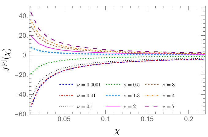
Figure 1: Variation of the jet function as a function of angle $\chi$ for various values of $\nu$. The medium parameters are $T=0.4$ GeV, $L=5$ fm and $m_{D}=0.8$ GeV.

Further for $\nu<1$ the jet function slowly approaches zero compared to $\nu>1$. As a consequence of this, the fixed order ratios of $\nu$-correlators are enhanced for $\nu<1$, which we will discuss shortly.

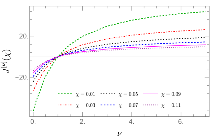
Figure 2: Variation of jet function as a function $\nu$ for various values of $\chi$. Here again the medium parameters are $L=5$ fm, $T=0.4$ GeV.

Next, in Figure 2, we plot the variation of the medium-induced jet function as a function of $\nu$ for various values of $\chi$ ranging from small to large. We observe that, similar to the vacuum case, the PE$\nu$C distributions become negative for the medium-induced case when $\nu<1$. However, unlike the vacuum case, this cannot be trivially mapped to the anomalous dimensions and we stress that such a mapping demands higher-order computations where we can explicitly see anomalous dimensions in the medium

Finally, to assess the relevance of $\nu$-correlators for various integer and non-integer values of $\nu$ in addition to the two-point correlators, we plot the ratios PE$\nu$C/PE2C at leading order for various values of $\nu$ in Figure 3. We find that for all values of $\nu>1$, the higher-point correlators are enhanced in the medium across the entire range of angular scales. Additionally, we observe a mild angular dependence in the ratio of these correlators when compared to the two-point case. In contrast, correlators with $\nu<1$ are much more interesting in the medium. For these small-$\nu$ values, we observe that not only the medium effects are enhanced but an intrinsic non-trivial dependence on the angular scale of the correlator also arises. In Sec. 4.2, we validate this finding also against the Monte-Carlo results obtained from JEWEL. Next, we analyze the impact of resummation on the results of the fixed order distributions presented so far.

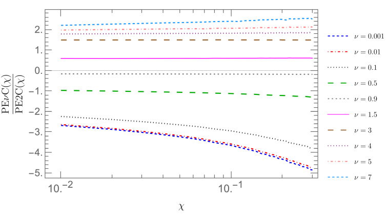
Figure 3: Variation of ratios of $\nu$-point energy correlators with that of $\nu=2$ as a function of angle $\chi$. Medium parameters are same as the one used in Figure 3.

From renormalization group (RG) consistency, we can infer that medium-induced jet function obeys a Balitsky-Fadin-Kuraev-Lipatov (BFKL) evolution equation with anomalous dimension same as the medium function but with an opposite sign [38]. Although, higher order computation of the jet function are necessary for the knowledge of the actual scale for BFKL evolution. To obtain the renormalized jet function we follow the prescription outlined in Ref. [64] to solve

$$\frac{d{\bf S}^{[\nu]}({\boldsymbol{k}},\nu^{\prime})}{d\ln\nu^{\prime}}\!=-\frac{\alpha_{s}(\mu)N_{c}}{\pi^{2}}\!\!\!\int\!d^{2}{\boldsymbol{u}}\bigg{[}\frac{{\bf S}^{[\nu]}({\boldsymbol{u}},\nu^{\prime})}{({\boldsymbol{u}}-{\boldsymbol{k}})^{2}}-\frac{{\boldsymbol{k}}^{2}{\bf S}^{[\nu]}({\boldsymbol{k}},\nu^{\prime})}{2{\boldsymbol{u}}^{2}({\boldsymbol{u}}-{\boldsymbol{k}})^{2}}\bigg{]},$$ (37)

where $\nu^{\prime}$ is the scale associated to rapidity renormalization and $\mu$ is the UV scale respectively. In order to solve the above evolution equation, one needs the precise knowledge of the rapidity scale for the jet function which for our case only appears at next-to-next-to-leading order (NNLO) which has not been computed so far. Nevertheless, to qualitatively capture the impact of resummation, we perform running from a scale $\nu^{\prime}_{0}\equiv Q_{{\rm med}}/\sqrt{\chi}$ to the medium scale $Q_{{\rm med}}\sim 3$ GeV. This yields

$${\bf S}^{[\nu]}_{\rm R}({\boldsymbol{k}})=\frac{1}{\pi|{\boldsymbol{k}}|}\sqrt{\frac{\pi}{14\zeta(3)\bar{\alpha}Y}}e^{(a_{p}-1)Y}\int d^{2}{\boldsymbol{u}}\frac{{\bf S}^{[\nu]}({\boldsymbol{u}})}{|{\boldsymbol{u}}|}e^{-\frac{\log^{2}(|{\boldsymbol{k}}|/|{\boldsymbol{u}}|)}{14\zeta(3)\bar{\alpha}Y}},$$ (38)

where $a_{p}=1+4\alpha_{s}N_{c}\ln{2}/\pi$ and $Y=\log(\nu^{\prime}_{0}/|{\boldsymbol{k}}|)$. The transverse momentum scale $|{\boldsymbol{k}}|\sim Q_{{\rm med}}$ so that $Y\sim\ln 1/\sqrt{\chi}$. We plot the variation of the ratio of resummed and leading jet function with $\chi$ in Figure 4. From the plot, we note a very mild dependence of the $\nu$-correlators with $\nu$. This is because, for resummed jet function, the only $\nu$ information is in the boundary condition (in Eq. 37) which is the fixed order jet function. However, in more realistic scenarios we also need the information of $\nu$ dependence of anomalous dimensions which only appears at NNLO.

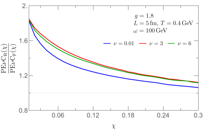
Figure 4: Variation of ratios of resummed and leading order jet functions as a function of angle $\chi$ for various values of $\nu$ and $\omega=100$ GeV.

4.2 JEWEL Analysis

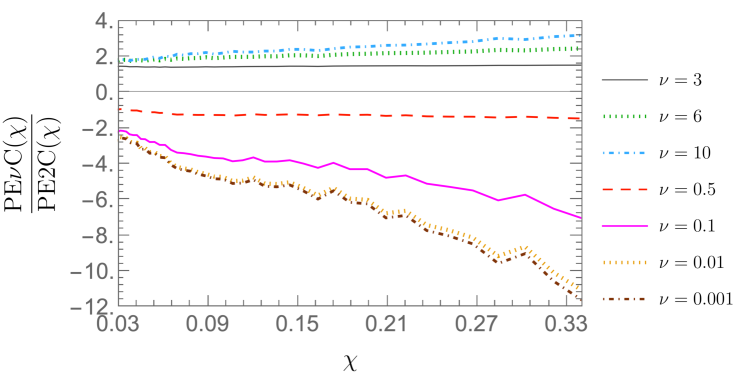
Figure 5: Ratios of PE$\nu$C distributions with respect to the 2-point distribution utilizing the data generated from JEWEL simulations.

Having established the features of the $\nu$-point projected correlators in our analytic framework, we now validate our results against Monte Carlo simulations generated with JEWEL [26, 65, 66, 67] in an idealized set-up (without recoils). The realistic case incorporating the default medium model in JEWEL as well as medium recoils is discussed in  B. In order to establish a fair comparison, we switch off all initial-state radiation, final-state radiation and multiple-parton interaction effects within PYTHIA 6.4 complemented with JEWEL. Further, we utilize a brick set-up of the medium and turn off the hadronization effects. The $\nu$-correlators are then computed on simulated events for $\sqrt{s_{NN}}=5.02$ TeV Pb+Pb collisions with a brick of length $L=9\,{\rm fm}$ and temperature $T=0.5\,{\rm MeV}$. Finally, we construct anti-kt jets with radius $R=0.4$ within the transverse momentum range $p_{T}\in[100,120]\,{\rm GeV}$ and psuedo-rapidity $|\eta|<1.9$. For practical purposes, we use the new method detailed in Ref. [68] and available through Refs. [69, 70], for the computation of $\nu$-correlators for various $\nu$ values.

The results for the ratios of PE$\nu$C to the two-point energy correlator are presented in Figure 5. From the figure, we note very similar qualitative features as observed in our analytic computation, namely $\nu\to 0$ exhibit an intrinsic angular dependence beyond what is contained by a two-point energy correlator.

5 Conclusions

In this Letter, we evaluated the analytic structure of general $\nu$-correlators, at the leading order in the QGP medium. Although $\nu$-correlators exhibit a classical scaling that goes like $1/\chi$ for all $\nu$-values in the vacuum, we analytically show that their structure is far more non-trivial in the case of the medium modified jets. A simple scaling behavior can be obtained only in very specific limits and phase-space regimes, for all the hierarchies we consider here. Additionally, in the vacuum, $\nu$-correlators are also interesting from a phenomenological point of view as they can not only provide an access to the leading twist collinear dynamics in jets but also allow the study of small-$x$ dynamics using jets. In HICs, we show that these correlators are interesting as they contain more angular information and hold the potential to fully unravel the medium effects through the use of the full $\nu$ dependent structure of these correlators.

On one hand, by studying the ratios of $\nu$-correlators relative to the simple two-point energy correlator, we find that although higher-point projected energy correlators are enhanced by the medium as seen from the numerical results in Figure 3 as well as JEWEL simulation in Figure 5, they encode somewhat similar angular information as the two-point energy correlator. On the other hand, our study reveals that $\nu<1$ correlators seem to be more interesting probes of the medium dynamics as they are not only enhanced by the medium but also encode non-trivial angular information compared to two-point as well as higher-point projected correlators. This is explicitly shown with a fitted form in Figure 6. We also note that for $\nu<1$, the $\nu$-correlators almost saturates at $\nu=0.01$ which we also show in Figure 3 as well as through analytic calculation given in Eq. 33. While these small-$\nu$ values are of interest, the complete potential of these correlators requires more detailed theoretical and phenomenological efforts and we hope our study provides a motivation towards such future investigations.

It is worth emphasizing that in the vacuum, the scaling of PE$\nu$C distributions is governed by the anomalous dimensions of the theory. However, in HICs, the scaling observed in the ratios of Figure 3 is not (yet) connected to medium evolution through anomalous dimensions but is inherently due to the non-trivial structure of the leading order medium-induced jet function. Higher order computations of the medium jet function are therefore necessary to truly exploit the structure of the medium evolution. Finally, we stress that, in this work, we restrict to the leading order jet function within the double Glauber insertion limit, a more detailed study that incorporates higher order contributions will certainly improve our understanding of jet dynamics in HICs.

Appendix A $\nu$-point angular Scalings

To obtain a simple angular scaling behavior of the ratios of PE$\nu$C distributions shown in Figure 3, we fit these ratios to a power law of form $a\chi^{b}$. The fit values for various $\nu$ values are tabulated in Table 1.

$\nu$	a	b	$\sim\chi^{b}$
0.01	5.74	0.19	$\chi^{0.19}$
3	1.87	0.01	$\chi^{0.01}$
6	2.68	0.04	$\chi^{0.04}$

Table 1: Approximate scaling for ratio of $\nu$-correlators with that of 2-point energy correlators. Here we take the same medium parameters as in Section 4.1.

For illustration purposes, we take the medium parameters as $L=5$ fm and $T=0.4$ GeV and only show the band with coupling variation $g=1.8-2.2$. We do not show the fit uncertainities here, although we have checked that these are not larger than the error bands that we choose to show in Figure 6. From the fit values, we again note that the correlator with $\nu=0.01$ has the strongest angular dependence when compared to other $\nu$ values considered in the plot.

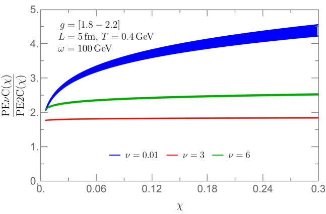
Figure 6: Approximate angular scaling behavior of $\nu$-point energy correlators for $\nu=0.01,3,6$ compared to $\nu=2$. Medium parameters are same as the one used in Figure 2.

Appendix B Full JEWEL simulation

In this section, we show the full JEWEL simulations for the ratios of $\nu$-correlators with that of the two-point correlator. For the plot shown in this section, we consider the default medium model encoded in JEWEL that incorporates a Bjorken-like expansion of the medium and consider the impact of recoil on the PE$\nu$C distributions. For medium distributions in the presence of recoil, we perform the constituent subtraction method for background subtraction as detailed in Ref. [67].

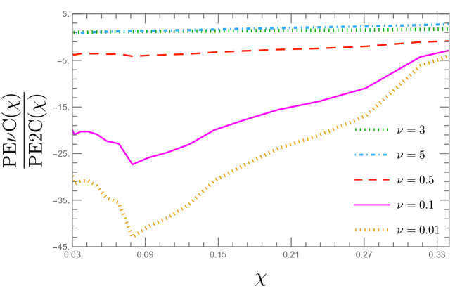
Figure 7: JEWEL simulation results incorporating medium recoil as well as hadronization effects.

The full simulation results are shown in Figure 7. These results highlight that the features observed in our simple analytic set-up for $\nu<1$ hold even in the light of a more realistic scenario.

References

- [1] G. P. Salam, Towards Jetography, Eur. Phys. J. C 67 (2010) 637–686. arXiv:0906.1833, doi:10.1140/epjc/s10052-010-1314-6.
- [2] M. Connors, C. Nattrass, R. Reed, S. Salur, Jet measurements in heavy ion physics, Rev. Mod. Phys. 90 (2018) 025005. arXiv:1705.01974, doi:10.1103/RevModPhys.90.025005.
- [3] U. A. Wiedemann, Gluon radiation off hard quarks in a nuclear environment: Opacity expansion, Nucl. Phys. B 588 (2000) 303–344. arXiv:hep-ph/0005129, doi:10.1016/S0550-3213(00)00457-0.
- [4] J.-P. Blaizot, F. Dominguez, E. Iancu, Y. Mehtar-Tani, Medium-induced gluon branching, JHEP 01 (2013) 143. arXiv:1209.4585, doi:10.1007/JHEP01(2013)143.
- [5] C. Andres, L. Apolinário, F. Dominguez, Medium-induced gluon radiation with full resummation of multiple scatterings for realistic parton-medium interactions, JHEP 07 (2020) 114. arXiv:2002.01517, doi:10.1007/JHEP07(2020)114.
- [6] S. Schlichting, I. Soudi, Medium-induced fragmentation and equilibration of highly energetic partons, JHEP 07 (2021) 077. arXiv:2008.04928, doi:10.1007/JHEP07(2021)077.
- [7] J. Casalderrey-Solana, E. Iancu, Interference effects in medium-induced gluon radiation, JHEP 08 (2011) 015. arXiv:1105.1760, doi:10.1007/JHEP08(2011)015.
- [8] A. M. Sirunyan, et al., Measurement of the Splitting Function in and Pb-Pb Collisions at 5.02 TeV, Phys. Rev. Lett. 120 (14) (2018) 142302. arXiv:1708.09429, doi:10.1103/PhysRevLett.120.142302.
- [9] X.-f. Guo, X.-N. Wang, Multiple scattering, parton energy loss and modified fragmentation functions in deeply inelastic e A scattering, Phys. Rev. Lett. 85 (2000) 3591–3594. arXiv:hep-ph/0005044, doi:10.1103/PhysRevLett.85.3591.
- [10] Y. Mehtar-Tani, Non-linear dynamics of jet quenching (11 2024). arXiv:2411.11992.
- [11] J.-P. Blaizot, F. Dominguez, E. Iancu, Y. Mehtar-Tani, Probabilistic picture for medium-induced jet evolution, JHEP 06 (2014) 075. arXiv:1311.5823, doi:10.1007/JHEP06(2014)075.
- [12] U. A. Wiedemann, Jet Quenching in Heavy Ion Collisions (2010) 521–562arXiv:0908.2306, doi:10.1007/978-3-642-01539-7_17.
- [13] A. Majumder, M. Van Leeuwen, The Theory and Phenomenology of Perturbative QCD Based Jet Quenching, Prog. Part. Nucl. Phys. 66 (2011) 41–92. arXiv:1002.2206, doi:10.1016/j.ppnp.2010.09.001.
- [14] Y. Mehtar-Tani, J. G. Milhano, K. Tywoniuk, Jet physics in heavy-ion collisions, Int. J. Mod. Phys. A 28 (2013) 1340013. arXiv:1302.2579, doi:10.1142/S0217751X13400137.
- [15] J. P. Blaizot, Y. Mehtar-Tani, Jet Structure in Heavy Ion Collisions, Int. J. Mod. Phys. E 24 (11) (2015) 1530012. arXiv:1503.05958, doi:10.1142/S021830131530012X.
- [16] G.-Y. Qin, X.-N. Wang, Jet quenching in high-energy heavy-ion collisions, Int. J. Mod. Phys. E 24 (11) (2015) 1530014. arXiv:1511.00790, doi:10.1142/S0218301315300143.
- [17] L. Apolinário, Y.-J. Lee, M. Winn, Heavy quarks and jets as probes of the QGP, Prog. Part. Nucl. Phys. 127 (2022) 103990. arXiv:2203.16352, doi:10.1016/j.ppnp.2022.103990.
- [18] A. Budhraja, M. van Leeuwen, J. G. Milhano, Jet observables in heavy ion collisions : a white paper (9 2024). arXiv:2409.03017.
- [19] M. Gyulassy, P. Levai, I. Vitev, Reaction operator approach to nonAbelian energy loss, Nucl. Phys. B 594 (2001) 371–419. arXiv:nucl-th/0006010, doi:10.1016/S0550-3213(00)00652-0.
- [20] L. D. Landau, I. Pomeranchuk, Limits of applicability of the theory of bremsstrahlung electrons and pair production at high-energies, Dokl. Akad. Nauk Ser. Fiz. 92 (1953) 535–536.
- [21] A. B. Migdal, Bremsstrahlung and pair production in condensed media at high-energies, Phys. Rev. 103 (1956) 1811–1820. doi:10.1103/PhysRev.103.1811.
- [22] C. Andres, L. Apolinário, F. Dominguez, M. G. Martinez, In-medium gluon radiation spectrum with all-order resummation of multiple scatterings in longitudinally evolving media, JHEP 11 (2024) 025. arXiv:2307.06226, doi:10.1007/JHEP11(2024)025.
- [23] M. Gyulassy, I. Vitev, X.-N. Wang, B.-W. Zhang, Jet quenching and radiative energy loss in dense nuclear matter (2004) 123–191arXiv:nucl-th/0302077, doi:10.1142/9789812795533_0003.
- [24] C. A. Salgado, U. A. Wiedemann, Medium modification of jet shapes and jet multiplicities, Phys. Rev. Lett. 93 (2004) 042301. arXiv:hep-ph/0310079, doi:10.1103/PhysRevLett.93.042301.
- [25] G.-Y. Qin, J. Ruppert, C. Gale, S. Jeon, G. D. Moore, M. G. Mustafa, Radiative and collisional jet energy loss in the quark-gluon plasma at RHIC, Phys. Rev. Lett. 100 (2008) 072301. arXiv:0710.0605, doi:10.1103/PhysRevLett.100.072301.
- [26] K. Zapp, G. Ingelman, J. Rathsman, J. Stachel, U. A. Wiedemann, A Monte Carlo Model for ’Jet Quenching’, Eur. Phys. J. C 60 (2009) 617–632. arXiv:0804.3568, doi:10.1140/epjc/s10052-009-0941-2.
- [27] J. Casalderrey-Solana, D. C. Gulhan, J. G. Milhano, D. Pablos, K. Rajagopal, A Hybrid Strong/Weak Coupling Approach to Jet Quenching, JHEP 10 (2014) 019, [Erratum: JHEP 09, 175 (2015)]. arXiv:1405.3864, doi:10.1007/JHEP09(2015)175.
- [28] Y. He, T. Luo, X.-N. Wang, Y. Zhu, Linear Boltzmann Transport for Jet Propagation in the Quark-Gluon Plasma: Elastic Processes and Medium Recoil, Phys. Rev. C 91 (2015) 054908, [Erratum: Phys.Rev.C 97, 019902 (2018)]. arXiv:1503.03313, doi:10.1103/PhysRevC.91.054908.
- [29] Y.-T. Chien, I. Vitev, Towards the understanding of jet shapes and cross sections in heavy ion collisions using soft-collinear effective theory, JHEP 05 (2016) 023. arXiv:1509.07257, doi:10.1007/JHEP05(2016)023.
- [30] X.-N. Wang, S.-Y. Wei, H.-Z. Zhang, Effect of medium recoil and broadening on single inclusive jet suppression in high-energy heavy-ion collisions in the high-twist approach, Phys. Rev. C 96 (3) (2017) 034903. arXiv:1611.07211, doi:10.1103/PhysRevC.96.034903.
- [31] Y. He, S. Cao, W. Chen, T. Luo, L.-G. Pang, X.-N. Wang, Interplaying mechanisms behind single inclusive jet suppression in heavy-ion collisions, Phys. Rev. C 99 (5) (2019) 054911. arXiv:1809.02525, doi:10.1103/PhysRevC.99.054911.
- [32] J. Casalderrey-Solana, G. Milhano, D. Pablos, K. Rajagopal, Modification of Jet Substructure in Heavy Ion Collisions as a Probe of the Resolution Length of Quark-Gluon Plasma, JHEP 01 (2020) 044. arXiv:1907.11248, doi:10.1007/JHEP01(2020)044.
- [33] P. Caucal, E. Iancu, G. Soyez, Deciphering the distribution in ultrarelativistic heavy ion collisions, JHEP 10 (2019) 273. arXiv:1907.04866, doi:10.1007/JHEP10(2019)273.
- [34] V. Vaidya, X. Yao, Transverse momentum broadening of a jet in quark-gluon plasma: an open quantum system EFT, JHEP 10 (2020) 024. arXiv:2004.11403, doi:10.1007/JHEP10(2020)024.
- [35] V. Vaidya, Effective Field Theory for jet substructure in heavy ion collisions, JHEP 11 (2021) 064. arXiv:2010.00028, doi:10.1007/JHEP11(2021)064.
- [36] A. Baty, P. Gardner, W. Li, Novel observables for exploring QCD collective evolution and quantum entanglement within individual jets, Phys. Rev. C 107 (6) (2023) 064908. arXiv:2104.11735, doi:10.1103/PhysRevC.107.064908.
- [37] L. Cunqueiro, A. M. Sickles, Studying the QGP with Jets at the LHC and RHIC, Prog. Part. Nucl. Phys. 124 (2022) 103940. arXiv:2110.14490, doi:10.1016/j.ppnp.2022.103940.
- [38] V. Vaidya, Radiative corrections for factorized jet observables in heavy ion collisions, JHEP 05 (2024) 028. arXiv:2107.00029, doi:10.1007/JHEP05(2024)028.
- [39] P. Caucal, A. Soto-Ontoso, A. Takacs, Dynamically groomed jet radius in heavy-ion collisions, Phys. Rev. D 105 (11) (2022) 114046. arXiv:2111.14768, doi:10.1103/PhysRevD.105.114046.
- [40] Y. Mehtar-Tani, D. Pablos, K. Tywoniuk, Cone-Size Dependence of Jet Suppression in Heavy-Ion Collisions, Phys. Rev. Lett. 127 (25) (2021) 252301. arXiv:2101.01742, doi:10.1103/PhysRevLett.127.252301.
- [41] A. Kumar, et al., Inclusive jet and hadron suppression in a multistage approach, Phys. Rev. C 107 (3) (2023) 034911. arXiv:2204.01163, doi:10.1103/PhysRevC.107.034911.
- [42] A. Budhraja, R. Sharma, B. Singh, Medium modifications to jet angularities using SCET with Glauber gluons (5 2023). arXiv:2305.10237.
- [43] S.-L. Zhang, E. Wang, H. Xing, B.-W. Zhang, Flavor dependence of jet quenching in heavy-ion collisions from a Bayesian analysis, Phys. Lett. B 850 (2024) 138549. arXiv:2303.14881, doi:10.1016/j.physletb.2024.138549.
- [44] J. a. Barata, J. G. Milhano, A. V. Sadofyev, Picturing QCD jets in anisotropic matter: from jet shapes to energy energy correlators, Eur. Phys. J. C 84 (2) (2024) 174. arXiv:2308.01294, doi:10.1140/epjc/s10052-024-12514-1.
- [45] Y. Mehtar-Tani, F. Ringer, B. Singh, V. Vaidya, Factorization for jet production in heavy-ion collisions (9 2024). arXiv:2409.05957.
- [46] B. Singh, V. Vaidya, Towards factorization with emergent scales for jets in dense media (12 2024). arXiv:2412.18967.
- [47] C. Andres, F. Dominguez, R. Kunnawalkam Elayavalli, J. Holguin, C. Marquet, I. Moult, Resolving the Scales of the Quark-Gluon Plasma with Energy Correlators, Phys. Rev. Lett. 130 (26) (2023) 262301. arXiv:2209.11236, doi:10.1103/PhysRevLett.130.262301.
- [48] Z. Yang, Y. He, I. Moult, X.-N. Wang, Probing the Short-Distance Structure of the Quark-Gluon Plasma with Energy Correlators, Phys. Rev. Lett. 132 (1) (2024) 011901. arXiv:2310.01500, doi:10.1103/PhysRevLett.132.011901.
- [49] C. Andres, F. Dominguez, J. Holguin, C. Marquet, I. Moult, A coherent view of the quark-gluon plasma from energy correlators, JHEP 09 (2023) 088. arXiv:2303.03413, doi:10.1007/JHEP09(2023)088.
- [50] J. a. Barata, P. Caucal, A. Soto-Ontoso, R. Szafron, Advancing the understanding of energy-energy correlators in heavy-ion collisions, JHEP 11 (2024) 060. arXiv:2312.12527, doi:10.1007/JHEP11(2024)060.
- [51] C. Andres, F. Dominguez, J. Holguin, C. Marquet, I. Moult, Towards an Interpretation of the First Measurements of Energy Correlators in the Quark-Gluon Plasma (7 2024). arXiv:2407.07936.
- [52] B. Singh, V. Vaidya, Factorization for energy-energy correlator in heavy ion collision (8 2024). arXiv:2408.02753.
- [53] J. a. Barata, M. V. Kuzmin, J. G. Milhano, A. V. Sadofyev, Jet EEC aWAKEning: hydrodynamic response on the celestial sphere (12 2024). arXiv:2412.03616.
- [54] J. a. Barata, R. Szafron, Leading order track functions in a hot and dense QGP, Phys. Rev. D 110 (3) (2024) L031501. arXiv:2401.04164, doi:10.1103/PhysRevD.110.L031501.
- [55] H. Bossi, A. S. Kudinoor, I. Moult, D. Pablos, A. Rai, K. Rajagopal, Imaging the wakes of jets with energy-energy-energy correlators, JHEP 12 (2024) 073. arXiv:2407.13818, doi:10.1007/JHEP12(2024)073.
- [56] J. a. Barata, I. Moult, J. a. M. Silva, Tracking Energy Loss in Heavy Ion Collisions (9 2024). arXiv:2409.18174.
- [57] J. a. Barata, I. Moult, A. V. Sadofyev, J. a. M. Silva, Dissecting Jet Modification in the QGP with Multi-Point Energy Correlators (3 2025). arXiv:2503.13603.
- [58] V. Vaidya, Probing a dilute short lived Quark Gluon Plasma medium with jets (9 2021). arXiv:2109.11568.
- [59] C. L. Basham, L. S. Brown, S. D. Ellis, S. T. Love, Energy Correlations in Perturbative Quantum Chromodynamics: A Conjecture for All Orders, Phys. Lett. B 85 (1979) 297–299. doi:10.1016/0370-2693(79)90601-4.
- [60] C. L. Basham, L. S. Brown, S. D. Ellis, S. T. Love, Energy Correlations in electron-Positron Annihilation in Quantum Chromodynamics: Asymptotically Free Perturbation Theory, Phys. Rev. D 19 (1979) 2018. doi:10.1103/PhysRevD.19.2018.
- [61] C. L. Basham, L. S. Brown, S. D. Ellis, S. T. Love, Energy Correlations in electron - Positron Annihilation: Testing QCD, Phys. Rev. Lett. 41 (1978) 1585. doi:10.1103/PhysRevLett.41.1585.
- [62] C. L. Basham, L. S. Brown, S. D. Ellis, S. T. Love, Electron - Positron Annihilation Energy Pattern in Quantum Chromodynamics: Asymptotically Free Perturbation Theory, Phys. Rev. D 17 (1978) 2298. doi:10.1103/PhysRevD.17.2298.
- [63] H. Chen, I. Moult, X. Zhang, H. X. Zhu, Rethinking jets with energy correlators: Tracks, resummation, and analytic continuation, Phys. Rev. D 102 (5) (2020) 054012. arXiv:2004.11381, doi:10.1103/PhysRevD.102.054012.
- [64] Y. V. Kovchegov, E. Levin, Quantum Chromodynamics at High Energy, Vol. 33, Oxford University Press, 2013. doi:10.1017/9781009291446.
- [65] K. C. Zapp, F. Krauss, U. A. Wiedemann, A perturbative framework for jet quenching, JHEP 03 (2013) 080. arXiv:1212.1599, doi:10.1007/JHEP03(2013)080.
- [66] K. C. Zapp, JEWEL 2.0.0: directions for use, Eur. Phys. J. C 74 (2) (2014) 2762. arXiv:1311.0048, doi:10.1140/epjc/s10052-014-2762-1.
- [67] R. Kunnawalkam Elayavalli, K. C. Zapp, Medium response in JEWEL and its impact on jet shape observables in heavy ion collisions, JHEP 07 (2017) 141. arXiv:1707.01539, doi:10.1007/JHEP07(2017)141.
- [68] S. Alipour-fard, A. Budhraja, J. Thaler, W. J. Waalewijn, New Angles on Energy Correlators (10 2024). arXiv:2410.16368.
- [69] A. Budhraja, W. Waalewijn, FastEEC 0.3, https://github.com/abudhraj/FastEEC/releases/tag/0.3 (2024).
- [70] S. Alipour-fard, ResolvedEnergyCorrelators (RENCs), https://github.com/samcaf/ResolvedEnergyCorrelators (2024).