Diffusion-aggregation equations and volume-preserving mean curvature flows
Abstract
The Patlak-Keller-Segel system of equations (PKS) is a classical example of aggregation-diffusion equation. It describes the aggregation of some organisms via chemotaxis, limited by some nonlinear diffusion. It is known that for some choice of this nonlinear diffusion, the PKS model asymptotically leads to phase separation and mean-curvature driven free boundary problems. In this paper, we focus on the Elliptic-Parabolic PKS model and we obtain the first unconditional convergence result in dimension and towards the volume preserving mean-curvature flow. This work builds up on previous results that were obtained under the assumption that phase separation does not cause energy loss in the limit. In order to avoid this assumption, we rely on Brakke type formulation of the mean-curvature flow and a reinterpretation of the problem as an Allen-Cahn equation with a nonlocal forcing term.
Key words. Chemotaxis, Singular limit, Mean curvature flow, Varifolds.
MSC codes. 35A15, 35K55, 53E10.
1 Introduction
1.1 The Patlak-Keller-Segel model
The classical parabolic-parabolic Patlak-Keller-Segel (PKS) system for chemotaxis with nonlinear diffusion can be written as:
| (1.1) |
In this model, is the density function of some organisms (such as bacteria or other types of cells) and denotes the concentration of a chemoattractant. The organisms are advected toward regions of higher concentration of the chemoattractant with proportionality constant . The parameter denotes the diffusivity of the chemoattractant and the constant denotes the destruction rate of the chemoattractant.
We note that the relaxation time of the organisms (the parameter in (1.1)) and that of the chemoattractant (the parameter ) have no reason to be equal and can in fact differ by several orders of magnitude. In this paper, we will consider the particular case
which leads to the elliptic-parabolic PKS model (note that formally at least, the results presented in this paper are generalizable to regimes in which the organisms reach their equilibrium much faster than the chemoattractant diffuses, though the rigorous analysis is much more challenging in that case). The opposite regime , yields the popular parabolic-elliptic PKS model in which the chemoattractant reaches its equilibrium much faster than the organisms. The well-posedness of the PKS model has received a lot of attention for a wide range of nonlinearity (see [23, 19, 35, 25] and the references therein). The nonlinear diffusion term in (1.1) takes into account the natural repulsive forces acting on the organisms and plays a very important role in our paper. A classical fact about the PKS model is that linear diffusion (which corresponds to with our notations) can lead to finite time blow up of the solution (), a phenomena which describes the concentration of the organisms [4]. We are not interested in this phenomena and we will consider models with stronger repulsion for large values of which do not lead to finite time blow-up. A common choice for this nonlinearity is the power law
which penalizes high densities of the organisms. For , it has been shown that concentration cannot occur and that solutions remain bounded in uniformly in time. Another interesting phenomena occurs when : Several recent work [26, 25, 33] have shown that in this case, not only do solutions remain bounded for all time, but they experience phase separation phenomena at appropriate time scale.
A possible microscopic interpretation of the model with large is that the organisms have some finite size and that overlapping is permitted, but heavily penalized. In the limit , we get a hard sphere - or incompressible - model in which overlapping is prohibited and the density must satisfy an a priori upper bound. This corresponds to the nonlinearity
The corresponding equation enforces the congestion constraint and requires the introduction of a pressure term (Lagrange multiplier) in the equation. Since is convex, we can define its subdifferential and rewrite the first equation in (1.1) as
where the condition can also be written as , and . We stress out the fact that this singular limit has the double effect of enforcing the constraint and eliminating all diffusion when . In this paper we will take a nonlinearity which combines some nonlinear diffusion for small value of together with the hard-sphere constraint : From now on, we take
| (1.2) |
Our goal is to show that phase separation takes place, resulting in the formation of high and low density regions separated by a sharp interface, and to characterize the evolution of that interface. A similar study was undertaken in several recent papers (see [26, 25, 33, 34]) for the parabolic-elliptic and elliptic-parabolic PKS model and recently extended to the full parabolic-parabolic model in [41]. As in these papers, we assume that a large number of individuals are observed from far away: We introduce a parameter that quantifies the large (initial) mass
and rescale the problem as follows:
In these new (macroscopic) variables, (1.1) becomes:
| (1.3) |
Here is a fixed domain (which has macroscopic size ). This system will be supplemented with no-flux boundary conditions on and with the initial conditions by given profiles now with normalized initial mass
| (1.4) |
We note that by redefining , , , we can rewrite (1.3) as
| (1.5) |
thus eliminating all the parameters with the exception of the relaxation time
As mentioned at the beginning of this introduction, this paper focuses on the case which describes a situation in which the organisms adapt instantly to the distribution of the chemoattractant . The equation for becomes elliptic and the effect of the initial condition is reduced to the mass condition (1.4). The goal of this paper is thus to investigate the asymptotic behavior as of the solution of:
| (1.6) |
with the boundary conditions ( being the outer unit normal vector of )
| (1.7) |
and the initial condition
This limit was previously studied in [34] where it was proved that for well prepared initial condition, both and converge strongly to a characteristic function and that the interface evolves according to the volume preserving mean-curvature flow
| (1.8) |
where is the outward normal velocity at a point of the boundary , is the mean curvature of and is a Lagrange multiplier associated to the constraint .
However, in [34] equation (1.8) was derived under an assumption on the convergence of the energy (see (1.21)) which we do not know how to establish a priori. The goal of this paper is to establish a similar result rigorously without this assumption and thus get the first unconditional convergence result in this direction.
A key idea in the paper - which we explain in the next section - is that (1.6) can be recast as a nonlocal Allen-Cahn equation. We will thus prove our result by adapting strategies developed for volume preserving Allen-Cahn equations to our model. This requires some delicate estimates that we derive by using the particular form of the nonlinearity (1.2).
1.2 A non-local Allen-Cahn equation
For a given , the equation for the density describes the instantaneous relaxation of the organisms toward an equilibrium that balances the repulsive effect of the pressure and the attractive effect of the chemo-attractant. It should be interpreted as describing the long time asymptotic of the corresponding evolution equation and is thus naturally supplemented with non-negativity and mass constraint, which can be summarized by requiring that . Here denotes the set of probability measures on that are absolutely continuous with respect to the -dimensional Lebesgue measure on (a measure in will always be identified with its density in this paper). For a given potential , the density is thus solution of
| (1.9) |
Solutions of (1.9) may not be unique, but the corresponding minimization problem
| (1.10) |
has a unique solution. This is immediate since when is given by (1.2), we can write (1.10) as the minimization of the uniformly convex energy on the convex set . To ensure that is not empty, we will always assume that
| (1.11) |
To justify the choice of the energy minimizer among all possible solutions of (1.9), we point out that when a linear diffusion is added to (1.9) (modeling some noise in the behavior of the organisms), it has a unique solution which is also the unique global minimizer. Because the global minimizer is stable with respect to the limit , our choice for can be seen as a consequence of a natural vanishing noise approximation.
Important facts about the minimization problem (1.10) will be recalled in Proposition 3, but for now, we just note that it allows us to define a map which identifies the density distribution of the organisms for a given distribution of the chemo-attractant. With this notation, we can rewrite (1.6) as a single (nonlocal) equation
| (1.12) |
This definition of is also consistent with the natural energy structure of the PKS model. Indeed, we recall that the Parabolic-Parabolic system (1.5) is associated with the energy
Because of the mass conservation property, the term only changes the energy by a constant, but it will play an important role later on. Not surprisingly, the Elliptic-Parabolic system (1.6) is in turn associated with the energy functional
| (1.13) |
The construction of a solution to (1.6) satisfying the appropriate energy inequality was carried out in [34] using the gradient flow structure of the equation. These results will be recalled in Proposition 4.
The study of the singular limit in [34] (see also [33, 26]) relies on the following observation: A simple arithmetic manipulation (complete the square) allows us to rewrite the energy as follows:
| (1.14) |
where
This potential is defined for , but we will extend its definition to by setting for . The definition of , (1.2), leads to:
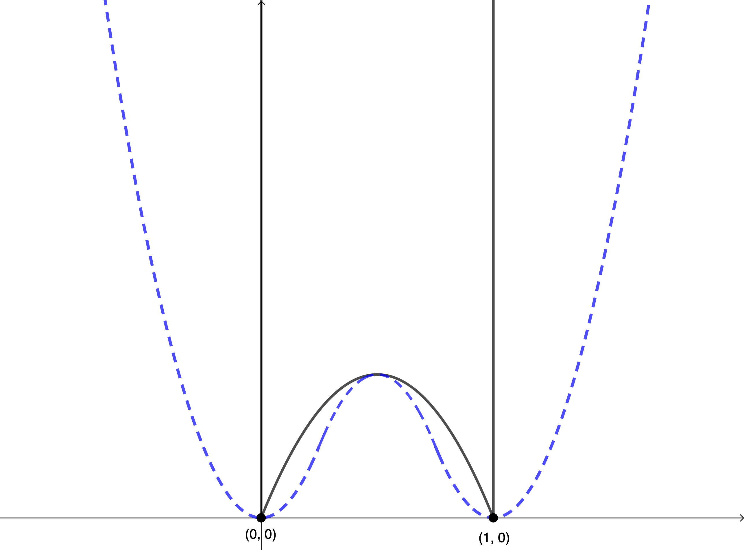
When , this function is convex but when , it is a double-well potential (see Figure 1) which satisfies
From now on, we will thus assume that the nonlinearity is given by (1.2) with
| (1.15) |
This ensures that the diffusion at low density is weaker than the attractive force when and is the key to observing phase-separation phenomena (when the limit leads to constant densities).
We now see that the energy (1.13) a structure reminiscent of the classical Allen-Cahn (or Modica-Mortola) functional, although the double-well potential acts on the density while the norm is that of the potential . We can make the connection a little bit more clear as follows: First (to simplify the notations), we introduce the function , also extended by for . The double-well potential can then be written as
and we introduce the dual potential
where denotes the Legendre transform333We recall that the Legendre transform is defined by of . With these notations, we can show the following:
Proposition 1.
The function is a double-well potential (see Figure 1) satisfying
The energy (1.13) can be written as follows:
| (1.16) |
For all , the solution of the minimization problem (1.10) is given by for some Lagrange multiplier .
Equation (1.12) can be rewritten as
| (1.17) |
where is a Lagrange multiplier defined by the constraint .
The proof of this proposition is straightforward and included in Appendix A for the reader’s sake. For future reference, we note that we have the explicit formula
| (1.18) |
and (using the definition of and the fact that ), we find that is a function whose derivative is given by the piecewise linear function
| (1.19) |
In the form (1.17), it is now clear that our equation has the form of a Allen-Cahn type equation with a double-well potential and a “forcing” term
which arises because of the density constraint (this term vanishes when the Lagrange multiplier is zero). Unlike the classical volume-preserving Allen-Cahn equation, this term does not directly enforce a condition on the integral of , but asymptotically (when ) we will see that the effect is the same. The singular limit of the Allen-Cahn equation with forcing term was studied in detailed in [37] under the condition
Proving that such a bound holds will be the most important step in our proof (see Proposition 7) and will requires a delicate control of the Lagrange multiplier . But once this is proved, we will be able to apply well known techniques and derive the mean-curvature flow equation (and prove our main result Theorem 1).
1.3 -convergence and conditional convergence result of [34]
All the terms in the energy (1.16) are non-negative since a function and its Legendre transform always satisfy
(with equality if and only if ). So the first term in (1.16) controls the convergence of to while the second integral in (1.16) is the classical Allen-Cahn energy (or Modica-Mortola functional) which is known to -converge to the perimeter functional. This gives the intuition behind the following proposition (see [34, 41] for the proof):
Proposition 2 (Theorem 2.3 in [34]).
This result will not play any role our analysis, but it justifies heuristicaly the presence of the mean-curvature operator in the limit . The derivation of the mean-curvature flow equation from (1.12) was established in [34] under the assumption of convergence of the energy. More precisely, the main result of [34] states that given a subsequence which converges to (such a subsequence exists), if we assume that
| (1.21) |
then the evolution of the interface is described by the volume preserving mean-curvature flow (1.8).
Similar conditional results were obtained in related framework in [26, 33, 34, 41] and in much broader contexts in [22, 39, 13, 29]. Since the -convergence guarantees that
we see that (1.21) holds if and only if there is no loss of energy in the limit. Such energy losses typically happen due to overlapping or disappearing interfaces in the limit process. In case of boundaries that overlap, for example, the left-hand side of (1.21) counts interfaces (at least) twice, while the right-hand side counts the interface only once.
In this paper, we will prove an unconditional convergence result. However, because the phenomena described above cannot be discounted, we will rely on a weaker notion of solution than that used in [34]: Following the work of Brakke [5] and Ilmanen [21] (see also [36, 37, 45, 46] for more recent work in this direction), we use a general notion of solutions using integral varifolds. More precisely, we will characterize the evolution of certain energy measures. Ideally, we expect these measures to coincide with the surface area measures associated with the interface separating regions with density and . However, in general these energy measures may be supported on hidden boundaries or take the multiplicity of the interface into account.
2 Preliminaries and main results
2.1 Well-posedness
We recall the following proposition (proved in [34] for smooth and in [41] for more general nonlinearities that include our function (1.2)):
Proposition 3.
For all , there exists a unique solution of (1.10). It satisfies .
The map is Lipschitz from with Lipschitz constant .
Next, we recall that the gradient flow structure of (1.12) was used in [34, Section 4] to prove the existence of a solution when is a smooth function. For the type of singular we are considering here this analysis was extended in [41]. We thus state the following well-posedness result without proof:
2.2 Basic definitions
Before we state our main result, we briefly recall some standard definitions from geometric measure theory (see [44] for more details):
We first recall that a Radon measure on is -rectifiable if for any for some countably -rectifiable and -measurable set and a function . We then write . We call the multiplicity and say that is -integral if the multiplicity is integer-valued -a.e. on .
For a Radon measure on and , if there exist a -dimensional linear subspace and a number such that
we say that has the approximate tangent plane , denoted by . Here, is the Lebesgue volume of the unit ball in . If a Radon measure on is -rectifiable, represented by with the above notations, then has the approximate plane at and at -a.e. .
For a -rectifiable Radon measure on with a locally finite, -rectifiable, and -measurable set and , we say that is a generalized mean curvature vector if
| (2.2) |
where is the approximate tangent space of at . We recall that for a -dimensional subspace of with an orthonormal basis and for a vector field , we have .
The notion of weak solution considered in this paper is based on the ideas introduced in the seminal work of Brakke [5] and Ilmanen [21] and requires the introduction of the notion of -flow (see [36]) which describes the evolution of integral varifolds with square integrable generalized mean-curvature and square integrable generalized velocity.
Definition 1 (-flow [36]).
Let be a family of -rectifiable Radon measures on such that has a generalized mean curvature vector for a.e. . We call an -flow if there exist a constant and a vector field such that
and
for any . Here, and is the approximate tangent space of at . A vector field satisfying the above conditions is called a generalized velocity vector.
We point out that any generalized velocity is (on a set of good points) uniquely determined by the evolution (see [36]).
2.3 Main results
Given a solution of (1.12) (or, equivalently (1.17)), we introduce the Radon measure on that expresses the total energy associated tothe Modica-Mortola functional:
with
Our main result is as follows:
Theorem 1.
Suppose and (1.11) holds. Let be given by (1.2), (1.15) and let be the solution to (1.12) with initial data , where the initial data satisfy .
Then, there exists a subsequence of (still denoted by ) such that
-
(A)
There exists a function (for all ) with
and such that
-
(A.i)
strongly in for any and in .
-
(A.ii)
with such that and for all .
-
(A.i)
-
(B)
There exists a family of -integral Radon measures on such that
-
(B.i)
as Radon measures on , where .
-
(B.ii)
as Radon measures on for all .
-
(B.iii)
for any and . Thus, for any .
-
(B.i)
-
(C)
There exists and a measurable function such that is an -flow with a generalized velocity vector such that
(2.3) where is the generalized mean-curvature vector defined by (2.2) and is the inner unit normal vector of on .
We make the following remarks:
- (i)
-
(ii)
We also note that Theorem 1 does not include any condition on the contact angle between the free boundary and the fixed boundary . The assumption (1.21) is used in [34] to derive a normal contact angle condition, which we are unable to recover here. This is a classical difficulty with this more general approach. For general contact angle conditions, still under (1.21), we refer to [18, 26].
The Lagrange multiplier will be obtained as the weak limit of
In fact, as in [45], the most delicate part of the proof is the derivation of appropriate estimates on the Lagrange multiplier term. A key role in this paper is played by the following proposition (proved in Section 3.2):
Proposition 5.
For all , there exists such that
In particular, there exists such that
2.4 A brief review of the literature
The volume preserving mean-curvature flow (1.8) is a classical free boundary problem. The existence of global-in-time classical solutions with convex smooth initial data was proved by Gage in [16] in 2-d and by Huisken in [20] in all dimensions. The short-time existence of classical solutions to (1.8) with smooth initial data (possibly nonconvex) was proved by Escher and Simonett [12]. Weak notions of solutions to (1.8) have also been studied: In [38], Mugnai, Seis and Spadaro proved the global existence of weak solutions in the sense of distributions in dimension using minimizing movement schemes (see also Luckhaus, Sturzenhecker [32]) under an assumption similar to (1.21). The convergence of thresholding schemes to distributional BV solutions of (1.8) was proved by Laux and Swartz [31] also under an assumption similar to (1.21). A similar approach was used by Laux and Simon [30] to prove the convergence of solutions of a multiphase mass-conserving Allen-Cahn equation toward the solution of a multiphase volume-preserving mean curvature flow. The weak-strong uniqueness for gradient-flow calibrations was proved by Laux [28].
Investigating sharp interface limits of Allen-Cahn-type equations has been a important subject as well. The classical Allen-Cahn equation [2] reads
with a double-well potential given by . The fact that the transition layer of converges to interfaces moving by mean curvature in the limit was justified in particular by Bronsard and Kon [7], Evans, Soner and Souganidis [14] (using viscosity solutions techniques - see also [11, 15]) and Ilmanen [21] using the notion of solutions introduced in Brakke’s seminal work [5]. We also refer to Chen [9] and references within for an extensive review of the literature on the Allen-Cahn equation. In [43], Sato gave a short proof of this convergence, using tools introduced by Röger and Schätzle in [40]. In [37], Mugnai and Röger extended this analysis to equations that include a forcing term:
using the concept of -flow that they developed in [36] (which we also use in this paper, see Definition 1) and which is similar to the notion of Brakke’s flow.
The volume preserving Allen-Cahn equation suggested by Rubinstein and Sternberg in [42], is given by
| (2.5) |
where is a Lagrange multiplier that enforces . Radially symmetric solutions to (2.5) were first studied by Bronsard and Stoth in [8], and Chen, Hilhorst and Logak [10] proved the convergence of the solution to (2.5) to the classical solution of (1.8) under the assumption that the latter exists.
An alternative Allen-Cahn equation with volume conservation was suggested by Golovaty [17] (see also Bretin and Brassel [6]):
| (2.6) |
In this model, the effect of the Lagrange multiplier is concentrated on the transition layer. In [1], Alfaro and Alifrangis proved that the solution of (2.6) converges to the classical solution of (1.8) if such a solution exists (Kroemer and Laux [27] obtained a rate of the convergence under the same assumption). In [45], Takasao proved the (unconditional) convergence for (2.6) in dimension using the same notion of weak solutions of (1.8) as in [36]. As far as we know, a similar result has not been obtained for (2.5) and the concentration of the Lagrange multiplier near the transition interface plays a crucial role in the proof. In [46] (motivated by [24, 38]) Takasao considered a slightly different choice of the multiplier which ensures a further regularity property, and obtained a similar convergence result in all dimensions.
Our equation bears some similarity with (2.6), especially obvious in its form (1.17), although we point out that the volume preservation of the limit comes from the mass preservation of since the volume of may not be preserved for a fixed . In [34], the second author and Rozowski showed the convergence of (1.6) to volume-preserving mean curvature flow (1.8) under the assumption of convergence of the energy (1.21). The present paper establishes the first unconditional convergence results for this problem, in the spirit of [37, 45].
3 Proof of Theorem 1
3.1 Phase separation
The first step is to prove that phase separation takes place in the limit . The following proposition is essentially Part (A) of Theorem 1. It’s proof is similar to the proof of [34, Proposition 6.1] and is recalled here for the sake of completeness.
Proposition 6.
Under the assumptions of Theorem 1, there exist a subsequence (still denoted by ) and a function (for all ) with
such that
-
(i)
strongly in for any and in .
-
(ii)
with such that and for all .
Proof.
Define the function by for and for . We let . Then, the Lipschitz continuity of gives
We note that, by (2.1) and (1.14) we have
Together with the mass constraint , we thus have . Also, by Young’s inequality,
Therefore, is bounded (uniformly in ) in .
Next, we see that since, for ,
Since is compactly embedded in for , a refined Aubin-Lions lemma (see [3, Theorem 1.1]) implies that is relatively compact in for and in for . Up to a subsequence, we can thus assume that converges to some function strongly in as for . The lower-semicontinuity of the -seminorm yields and .
Now, we claim that
Indeed, the function vanishes at , which are precisely the zeroes of . Since is bounded, for each , there exists a constant such that
where . Therefore, it holds (using (2.1), (1.13)) that
Taking and in turn, we obtain that Therefore, the convergence of to implies that of for . Furthermore Fatou’s lemma implies
and so the limit is a characteristic function with values for each . Writing , we see that since we already know . Finally, again by (2.1), (1.13), we have
This in particular implies that converges to in for , and that for each ,
which complete the proof. ∎
3.2 -estimate on the forcing term
The crucial estimate that we need to establish in order to use well-known machinery is an bound on the last term (the “Lagrange multiplier” term) in our equation (1.17) which we recall here for convenience:
| (3.1) |
with such that . The main result of this section and cornerstone of the paper is the following:
Proposition 7.
Under the assumptions of Theorem 1, there exists such that
The proof of this proposition relies on two facts: First, the fact that the rescaled Lagrange multiplier can be controlled in uniformly in space (it does not depend on ), and second, the concentration effect of the multiplier on the transition layer, which follows from the observation that
and allows us to use the energy to get some control in uniformly in time.
The first step is to establish the following -estimate for the Lagrange multiplier
Lemma 1.
Under the assumptions of Theorem 1, there exists such that
Proof.
We begin by multiplying (3.1) by where is a test vector field in with on . We obtain
A couple of integration by parts yield:
and
Since , the Fenchel-Young identity gives
We can thus write
Putting every together, we find the equality
All the terms in this equality with the exception of the last one, can be bounded by either the energy (1.16) or the dissipation of energy
In particular the definition of implies
Proceeding similarly with the other terms, we deduce:
| (3.2) |
The rest of the proof follows that of [34, Proposition 8.2] and we give a brief sketch here for the reader’s sake.
In view of (3.2), we can get a -bound on if we have a uniform lower bound of . Set , which is a positive number by (1.11). For a fixed , we claim that we can find a vector field with on such that
Indeed, we take a sequence of smooth functions such that converges to strongly in , for all , and and define , where solves the Neumann boundary problem
Then, we have and on . Moreover, by Proposition 6(ii),
We can thus set with a sufficiently large so that .
We now turn to the proof of Proposition 7 which combines the previous estimates with a localisation property of the function . This last property requires in a critical way the very particular choice of nonlinearity (1.2) that we made in this paper.
Proof of Proposition 7.
We recall that our choice of nonlinearity (1.2) and the definition of implies the following explicit formula for :
In particular we note that in with and so
| (3.3) |
For a fixed , we define
Then for , (3.3) gives:
The explicit formula for above gives and the definition of implies
with
We thus have
for some constant depending on , and . Using Lemma 1 we deduce that
| (3.4) |
for .
In order to control the integral over and complete the proof, we will first show that
| (3.5) |
For this, we recall that minimizes with the constraint , and we denote by the minimizer of the same functional without any mass constraint.
The formulation of the energy (1.14) gives
which implies
| (3.6) |
Next, we note that we also have
So we also have
| (3.7) |
Combining (3.6) and (3.7) gives (3.5) which in turn implies
Finally, Chebychev’s inequality gives
Using Lemma 1 we deduce that
for .
Together with (3.4), this implies the result. ∎
3.3 End of the proof of Theorem 1
Thanks to the bound proved in Proposition 7, we can use well established tools for Allen-Cahn equation with forcing terms to complete the proof of Theorem 1. We summarize below the results that we will need, which can be found in [40, Theorem 4.1, Proposition 4.9] and [37, Theorem 3.1, Proposition 4.4] (see also [45, Theorem 4.1]).
Theorem 2.
[40, 37] Suppose and let be a solution of the perturbed Allen-Cahn equation
| (3.8) |
where satisfies . We define
for and . Suppose that there exists such that
| (3.9) |
Then, there exists a subsequence of (still denoted by ) such that
-
(a)
There exists a family of -integral Radon measures on such that
-
(a.i)
as Radon measures on , where .
-
(a.ii)
as Radon measures on for all .
-
(a.i)
-
(b)
There exists such that
(3.10) -
(c)
is an -flow with a generalized velocity vector
and
Here, is the generalized mean curvature vector of and
Proof of Theorem 1.
Next, we use the formulation (1.17) of the equation to prove Parts (B) and (C): we see that solves (3.8) with forcing term
This term satisfies the following bound (see Proposition 7):
for some . Finally, (1.16) gives
We thus see that under the assumption of Theorem 1, the condition(3.9) is satisfied with and we can use Theorem 2 to complete the proof of our main result:
In particular, it is clear that Part (a) of Theorem 2 implies Part (B.i) and (B.ii) of Theorem 1 (the convergence of and as Radon measures). To prove (B.iii) of Theorem 1, we define the function by for and for , and we let . Then, for any , we see that as strongly in by Part (A) and by the Lipschitz continuity of , and therefore by the semicontinuity,
for any . This implies that .
We now turn to the proof of Part (C) of our theorem and the derivation of the mean-curvature flow equation. First, we note that the bound of Lemma 1 implies that (up to another subsequence) we can assume
Next, we need to identify the limiting force field defined by (3.10). This will follow from the following lemma:
Lemma 2.
We have
| (3.11) |
for any with on .
Postponing the proof of this lemma to the end of this section, we note that it implies (together with (3.10))
From the absolute continuity of with respect to proven in (B.iii) for a fixed , there is a density function . We thus can write
On , we have , and thus, . On , we have , and thus, is defined, and
Moreover, the function on is integer-valued due to the integrality of .
Part (c) of Theorem 2 now yields the conclustion that is an -flow with the generalized velocity vector
∎
Remark 1.
Appendix A Proof of Proposition 1
Proof of Proposition 1.
First, we note that we have the following alternate formula for :
| (A.1) |
Indeed, we have and so
Together with the fact that is a double well potential, (A.1) readily implies that and iff or . The explicit formula (1.19) for shows that is Lipschitz and so is .
The minimization problem (1.10) can be recast as
Since is convex, classical arguments implies that there exists a Lagrange multiplier such that or equivalently .
References
- [1] Mattieu Alfaro and Pierre Alifrangis. Convergence of a mass conserving allen-cahn equation whose lagrange multiplier is nonlocal and local. Interfaces Free Bound., 16(2):243–268, 2014.
- [2] Samuel Allen and John W. Cahn. A microscopic theory for antiphase boundary motion and its application to antiphase domain coarsening. Acta Metallurgh, 27:2789–2796, 1979.
- [3] Herbert Amann. Compact embeddings of vector-valued sobolev and besov spaces. Glas. Mat., 35(1):161–177, 2000.
- [4] Jacob Bedrossian, Nancy Rodriguez, and Andrea L. Bertozzi. Local and global well-posedness for aggregation equations and patlak–keller–segel models with degenerate diffusion. Nonlinearity, 24(6), 2011.
- [5] Kenneth Brakke. The motion of a surface by its mean curvature. Princeton University Press, 1978.
- [6] Elie Bretin and Morgan Brassel. A modified phase field approximation for mean curvature flow with conservation of the volume. Math. Methods Appl. Sci., 34(10):1157–1180, 2011.
- [7] Lia Bronsard and Robert V. Kohn. Motion by mean curvature as the singular limit of Ginzburg-Landau dynamics. J. Differential Equations, 90(2):211–237, 1991.
- [8] Lia Bronsard and Barbara Stoth. Volume-preserving mean curvature flow as a limit of a nonlocal Ginzburg-Landau equation. SIAM J. Math. Anal., 28(4):769–807, 1997.
- [9] Xinfu Chen. Global asymptotic limit of solutions of the cahn-hilliard equation. J. Differential Geometry, 44:262–311, 1996.
- [10] Xinfu Chen, Danielle Hilhorst, and Elisabeth Logak. Mass conserving allen-cahn equation and volume preserving mean curvature flow. Interfaces Free Bound., 12(4):527–549, 2010.
- [11] Yun-Gang Chen, Yoshikazu Giga, and Shun’ichi Goto. Uniqueness and existence of viscosity solutions of generalized mean curvature flow equations. J. Differential Geom., 33(3):749–786, 1991.
- [12] Joachim Escher and Gieri Simonett. The volume preserving mean curvature flow near spheres. Proc. Amer. Math. Soc., 126(9):2789–2796, 1998.
- [13] Selim Esedolu and Felix Otto. Threshold dynamics for networks with arbitrary surface tensions. Comm. Pure Appl. Math., 68(5):808–864, 2015.
- [14] Lawrence C. Evans, Halil M. Soner, and Panagiotis E. Souganidis. Phase separations and generalized motion by mean curvature. Comm. Pure Appl. Math., 45:1097–1123, 1992.
- [15] Lawrence C. Evans and Joel Spruck. Motion of level sets by mean curvature. i. J. Differential Geom., 33(3):635–681, 1991.
- [16] Michael Gage. On an area-preserving evolution equation for plane curves, volume 51. American Mathematical Society, 1986.
- [17] Dmitry Golovaty. The volume-preserving motion by mean curvature as an asymptotic limit of reaction-diffusion equations. Quart. Appl. Math., 55(2):243–298, 1997.
- [18] Sebastian Hensel and Tim Laux. BV solutions for mean curvature flow with constant contact angle: Allen-Cahn approximation and weak-strong uniqueness. Indiana Univ. Math. J., 73(1):111–148, 2024.
- [19] Miguel A. Herrero and Juan J. L. Velázquez. Chemotactic collapse for the keller-segel model. Journal of Mathematical Biology, 35(2):177–194, 1996.
- [20] Gerhard Huisken. The volume preserving mean curvature flow. J. reine angew. Math., 382:35–48, 1987.
- [21] Tom Ilmanen. Convergence of the allen-cahn equation to brakke’s motion by mean curvature. J. Differential Geom., 38(2):417–461, 1993.
- [22] Matt Jacobs, Inwon Kim, and Alpár R. Mészáros. Weak solutions to the muskat problem with surface tension via optimal transport. Arch. Rational Mech. Anal., 239(1):389–430, 2021.
- [23] Willi Jäger and Stephan Luckhaus. On explosions of solutions to a system of partial differential equations modelling chemotaxis. Trans. Amer. Math. Soc., 329(2):819–824, 1992.
- [24] Inwon Kim and Dohyun Kwon. Volume preserving mean curvature flow for star-shaped sets. Calc. Var. Partial Differential Equations, 59(81), 2020.
- [25] Inwon Kim, Antoine Mellet, and Jeremy S.-H. Wu. Aggregation-diffusion phenomena: from microscopic models to free boundary problems. arXiv:2401.01840, 2024.
- [26] Inwon Kim, Antoine Mellet, and Yijing Wu. Density-constrained chemotaxis and hele-shaw flow. Tran. Amer. Math. Soc., 377(1):395–429, 2024.
- [27] Milan Kroemer and Tim Laux. Quantitative convergence of the nonlocal allen-cahn equation to volume-preserving mean curvature flow. Math. Ann., 2024.
- [28] Tim Laux. Weak-strong uniqueness for volume-preserving mean curvature flow. Rev. Mat. Iberoam., 40(1):93–110, 2024.
- [29] Tim Laux and Felix Otto. Convergence of the thresholding scheme for multi-phase mean-curvature flow. Calc. Var. Partial Differential Equations, 55(1):1–74, 2016.
- [30] Tim Laux and Theresa M. Simon. Convergence of allen-cahn equation to multiphase mean curvature flow. Calc. Var. Partial Differential Equations, 71(8):1597–1647, 2018.
- [31] Tim Laux and Drew Swartz. Convergence of thresholding schemes incorporating bulk effects. Interfaces Free Bound., 19(2):273–304, 2017.
- [32] Stephan Luckhaus and Thomas Sturzenhecker. Implicit time discretization for the mean curvature flow equation. Calc. Var. Partial Differential Equations, 3(2):253–271, 1995.
- [33] Antoine Mellet. Hele-Shaw flow as a singular limit of a Keller-Segel system with nonlinear diffusion. Calc. Var. Partial Differential Equations, 63(8):Paper No. 214, 27, 2024.
- [34] Antoine Mellet and Michael Rozowski. Volume-preserving mean-curvature flow as a singular limit of a diffusion-aggregation equation. arXiv:2408.14309, 2024.
- [35] Yoshifumi Mimura. The variational formulation of the fully parabolic keller-segel system with degenerate diffusion. J. Differential Equations, 263(2):1477–1521, 2017.
- [36] Luca Mugnai and Matthias Röger. The Allen-Cahn action functional in higher dimensions. Interfaces and Free Boundaries, 10(1):45–78, 2008.
- [37] Luca Mugnai and Matthias Röger. Convergence of perturbed Allen-Cahn equations to forced mean curvature flow. Indiana Univ. Math. J., 60(1):41–75, 2011.
- [38] Luca Mugnai, Christian Seis, and Emanuele Spadaro. Global solutions to the volume-preserving mean-curvature flow. Calc. Var. Partial Differential Equations, 55(18), 2016.
- [39] Felix Otto. Dynamics of labyrinthine pattern formation in magnetic fluids: a mean-field theory. Arch. Rational Mech. Anal., 141(1):63–103, 1998.
- [40] Matthias Röger and Reiner Schätzle. On a modified conjecture of De Giorgi. Math. Z., 254(4):675–714, 2006.
- [41] Michael Rozowski. Hele-shaw flow with surface tension and kinetic undercooling as a sharp interface limit of the fully parabolic keller-segel system with nonlinear diffusion. in preparation.
- [42] Jacob Rubinstein and Peter Sternberg. Nonlocal reaction-diffusion equations and nucleation. IMA J. Appl. Math., 48(3):249–264, 1992.
- [43] Norifumi Sato. A simple proof of convergence of the Allen-Cahn equation to Brakke’s motion by mean curvature. Indiana Univ. Math. J., 57(4):1743–1751, 2008.
- [44] Leon Simon. Lectures on Geometric Measure Theory, volume 3. Proceedings of the Centre for Mathematics and its Applications, Australian National University, 1983.
- [45] Keisuke Takasao. Existence of weak solution for volume preserving mean curvature flow via phase field method. Indiana Univ. Math. J., 66(6):2015–2035, 2017.
- [46] Keisuke Takasao. The existence of a weak solution to volume preserving mean curvature flow in higher dimensions. Arch. Rational Mech. Anal., 247(52), 2023.