Bridging the Gap Between Contextual and Standard Stochastic Bilevel Optimization

Abstract

Contextual Stochastic Bilevel Optimization (CSBO) extends standard Stochastic Bilevel Optimization (SBO) by incorporating context-specific lower-level problems, which arise in applications such as meta learning and hyper-parameter optimization. This structure imposes an infinite number of constraints - one for each context realization - making CSBO significantly more challenging than SBO as the unclear relationship between minimizers across different contexts suggests computing numerous lower-level solutions for each upper-level iteration. Existing approaches to CSBO face two major limitations: substantial complexity gaps compared to SBO and reliance on impractical conditional sampling oracles. We propose a novel reduction framework that decouples the dependence of the lower-level solution on the upper-level decision and context through parametrization, thereby transforming CSBO into an equivalent SBO problem and eliminating the need for conditional sampling. Under reasonable assumptions on the context distribution and the regularity of the lower-level, we show that an $\epsilon$-stationary solution to CSBO can be achieved with a near-optimal sampling complexity $\tilde{\mathcal{O}}(\epsilon^{-3})$. Our approach enhances the practicality of solving CSBO problems by improving both computational efficiency and theoretical guarantees.

1 Introduction

We consider the following Contextual Stochastic Bilevel Optimization problem (CSBO):

$$\min_{x\in R^{d_{x}}}\quad F(x)\triangleq\mathbb{E}_{(\xi,\eta)\sim\mathbb{P}_{(\xi,\eta)}}\left[f(x,y^{\star}(x,\xi),\xi,\eta)\right]$$ (CSBO)

s.t. $$y^{\star}(x,\xi)=\operatorname*{arg\,min}_{y\in\mathbb{R}^{d_{y}}}\mathbb{E}_{\eta\sim\mathbb{P}_{\eta|\xi}}\left[g(x,y,\xi,\eta)\right],$$

$$\hskip 113.81102pt\forall x\in\mathbb{R}^{d_{x}},\xi\in\Xi$$

where $\mathbb{P}_{(\xi,\eta)}$ denotes the joint distribution of $\xi\in\mathbb{R}^{d_{\xi}}$ and $\eta\in\mathbb{R}^{d_{\eta}}$, and $\mathbb{P}_{\eta|\xi}$ denotes the distribution of $\eta$ conditioned to $\xi$. Here, $\Xi\subseteq\mathbb{R}^{d_{\xi}}$ is the support of the random variable $\xi$. The dimension of the upper and lower-level variables $x$ and $y$ are $d_{x}$ and $d_{y}$, respectively. The function $f(x,y,\xi,\eta)$ can be nonconvex in $x$, but $g(x,y,\xi,\eta)$ must be strongly convex with respect to $y$ for any given $x$, $\xi$, and $\eta$. Therefore, the minimizer of the lower-level, $y^{\star}(x,\xi)$, is unique for any $x$ and $\xi$. We aim to design a framework that leverages existing algorithms to obtain an $\epsilon$-accurate stationary point $x^{\star}$ i.e. satisfying $\mathbb{E}\|\nabla F(x^{\star})\|^{2}\leq\epsilon^{2}$, where the expectation is taken over the randomness of the algorithm producing $x^{\star}$.

Stochastic Bilevel Optimization (SBO) is a special case of CSBO where the lower level does not depend on $\xi$, in which case the solution to the lower level $y^{\star}$ depends only on $x$. Several papers have proposed solutions to SBO problems with a sample complexity in $\tilde{\mathcal{O}}(\epsilon^{-4})$ (Ji et al., 2021; Chen et al., 2022). Using variance reduction methods, sample complexities in $\tilde{\mathcal{O}}(\epsilon^{-3})$ (Guo et al., 2021; Khanduri et al., 2021; Yang et al., 2023) or even $\mathcal{O}(\epsilon^{-3})$ (Chu et al., 2024) have been achieved. More importantly, variance reduction methods yield algorithms achieving near-optimal complexity for SBO since optimal algorithms for single-level stochastic optimization find an $\epsilon$-stationary solution in $\mathcal{O}(\epsilon^{-3})$ (Fang et al., 2018; Cutkosky & Orabona, 2019; Arjevani et al., 2022).

Algorithms for SBO can be naively adapted to solve CSBO for finding an $\epsilon$-stationnary solution, i.e., for any iterate $x_{k}$, we solve $\Theta\left(\epsilon^{-2}\right)$ lower level problems to estimate $y^{\star}(x_{k},\xi)$. Specifically, using this naive approach to solve CSBO problems, the sample complexity of SBO algorithms ramps up from $\tilde{\mathcal{O}}(\epsilon^{-4})$ to $\tilde{\mathcal{O}}(\epsilon^{-6})$, and from $\tilde{\mathcal{O}}(\epsilon^{-3})$ to $\tilde{\mathcal{O}}(\epsilon^{-5})$ with variance reduction methods. Using multilevel Monte Carlo methods, (Hu et al., 2023b) reduces the sample complexity to $\tilde{\mathcal{O}}(\epsilon^{-4})$. However, the performance of their algorithm suffers when $y^{\star}(x,\xi)$ varies significantly with $\xi$. The latter is a shortcoming shared with the adaptation of (Finn et al., 2017) to SBO, and follows from the fact that $y^{\star}(x,\xi)$ is estimated from a reference point $y_{0}(x)$ shared across all $\xi$. Thus, their estimation of $y^{\star}(x,\xi)$ can be inaccurate or expensive when $y^{\star}(x,\xi)$ differs significantly from $y_{0}(x)$. In the specific case where $\Xi$ is discrete and of finite cardinality $m$, (Guo et al., 2021) achieves a sample complexity in $\tilde{\mathcal{O}}(m\epsilon^{-3})$. As such, their approach is not amenable to settings where $\xi$ is continuous. In addition, all of the above algorithms require a sampling oracle from the conditional distribution $\mathbb{P}_{\eta|\xi}$ which can be impractical if $\xi$ is continuous or has large support.

Therefore, the gap between the results of SBO and CSBO remains significant in the literature. Specifically, methods for solving CSBO suffer from at least one of the following drawbacks for continuous $\xi$:

1. The high sampling complexity compared to SBO by a factor $\tilde{\mathcal{O}}(\epsilon^{-1})$.

2. The requirement from the impractical sampling oracle from the conditional distribution $\mathbb{P}_{\eta|\xi}$.

This leaves an important question unanswered: Is it possible to close the gap between CSBO and SBO? Under mild additional regularity assumptions on $g$ and the distribution $\mathbb{P}_{\xi}$, we show not only that it is indeed possible to achieve a sampling complexity in $\tilde{\mathcal{O}}(\epsilon^{-3})$ for CSBO, but also that this is possible only by sampling from the joint distribution $\mathbb{P}_{(\xi,\eta)}$.

Notice that the main difficulty of (CSBO) comes from the coupling of $x$ and $\xi$ in the lower level solution $y^{\star}(x,\xi)$. To overcome this difficulty, we propose to decouple these two variables. Specifically, we parameterize $y^{\star}(x,\xi)$ as $y_{\Phi}(W(x),\xi)\triangleq W(x)\Phi(\xi)$, where $\Phi$ is a well-chosen vector of $N_{\Phi}(\epsilon)$ basis functions and $W(x)\in\mathbb{R}^{d_{y}\times N}$. We then consider the following SBO problem:

$$\min_{x\in\mathbb{R}^{d_{x}}}\quad F_{\Phi}(x)\triangleq\mathbb{E}_{(\xi,\eta)\sim\mathbb{P}_{(\xi,\eta)}}\left[f_{\Phi}(x,W^{\star}(x),\xi,\eta)\right] \text{SBO}_{\Phi}$$ ()

s.t. $$W^{\star}(x)=\!\!\!\!\operatorname*{arg\,min}_{W\in\mathbb{R}^{d_{y}\times N_{\Phi}(\epsilon)}}\!\!\!\mathbb{E}_{(\xi,\eta)\sim\mathbb{P}_{(\xi,\eta)}}\!\left[g_{\Phi}(x,W,\xi,\eta)\right],$$

$$\hskip 162.18062pt\forall x\in\mathbb{R}^{d_{x}}$$

where $f_{\Phi}(x,W,\xi,\eta)\triangleq f(x,y_{\Phi}(W,\xi),\xi,\eta)$ and $g_{\Phi}(x,W,\xi,\eta)\triangleq g(x,y_{\Phi}(W,\xi),\xi,\eta)$. Importantly, the linearity of the parametrization $y_{\Phi}$ in $W$ allows to transfer the convexity of $g$ in $y$ to $g_{\Phi}$ in $W$.

As depicted in Figure 1, our framework first consists in using the basis functions of $\Phi$ to construct an instance of SBO, ($\text{SBO}_{\Phi}$), that is closely related to (CSBO). Using existing algorithm for SBO, we find an $\epsilon$-accurate solution to ($\text{SBO}_{\Phi}$), which is then used to reconstruct a solution to (CSBO) that is $\epsilon$-accurate if $\Phi$ is well chosen. Our work focuses on relating the regularities of ($\text{SBO}_{\Phi}$) and the optimality gap of the reconstructed solution to simple metrics on $\Phi$, providing insights into how to choose $\Phi$ to achieve $\epsilon$-accurate solutions in near-optimal sample complexity.

Figure 1: Reduction framework.

Main Contributions

• We develop a reduction framework for CSBO that exploits the efficiency of existing SBO algorithms. We show that when $\Phi$ is sufficiently expressive, the reconstructed solution to (CSBO) is a valid $\epsilon$-stationary solution (Theorem 4.2). We then demonstrate that the regularity constants of ($\text{SBO}_{\Phi}$), and thus its sample complexity, are directly related to simple metrics on $\Phi$ (Theorem 4.5). Additionally, ($\text{SBO}_{\Phi}$) only uses samples from the joint distribution $\mathbb{P}_{(\xi,\eta)}$ so that (CSBO) can be solved without sampling from the impractical conditional distribution $\mathbb{P}_{\eta|\xi}$.

• Under mild additional assumptions on $g$ and $\mathbb{P}_{\xi}$ (Assumption 4.7), we show that for a specific choice of $\Phi$ encoding multivariate Chebyshev polynomials, our framework finds $\epsilon$-stationary solutions to (CSBO) in $\tilde{\mathcal{O}}(\epsilon^{-3})$ iterations and sample complexity (Corollary 4.9). In particular, our framework gives a sample complexity for CSBO that is an order of magnitude lower than that of state-of-the-art CSBO algorithms, and matches the lower bound of sample complexity for nonconvex stochastic optimization up to a logarithmic factor.

• Through numerical experiments in hyper-parameter optimization, we demonstrate the practical performance of our framework, achieving the best convergence rate and final loss compared to competing algorithms. The experiment also highlights the improved flexibility of our method in allocating resources to contexts that require them most.

2 Related Work

Our work lies at the intersection of three lines of work: Stochastic Bilevel Optimization, Contextual Optimization, and Approximation Theory.

Stochastic Bilevel Optimization

First introduced by (Bracken & McGill, 1973), SBO has been widely studied in the literature. Recent advancements have focused on the non-asymptotic analysis of stochastic gradient methods (Ghadimi & Wang, 2018; Chen et al., 2021; Khanduri et al., 2021; Hong et al., 2023; Kwon et al., 2024; Chen et al., 2024). Building on this, (Hu et al., 2023b) introduced the concept of Contextual Stochastic Bilevel Optimization, which generalizes SBO by incorporating a lower-level problem that depends on a context. Expanding on this concept, we introduce a more efficient and practical framework for tackling CSBO problems. Unlike existing approaches that adapt SBO algorithms to tackle CSBO, our approach reduces CSBO to SBO thereby enabling the use of any SBO algorithm, including first order methods (Chen et al., 2023; Kwon et al., 2023; Lu & Mei, 2024), and yielding near-optimal sampling complexity using state of the art algorithms for SBO (Guo et al., 2021; Khanduri et al., 2021).

Contextual Optimization

Another closely related line of work is Contextual Optimization (CO) where a risk-neutral decision-maker seeks to determine an optimal action $z^{\star}(x)$ that minimizes the expected costs conditioned on the covariate $x$. A comprehensive review of CO can be found in the survey by (Sadana et al., 2024). CO closely resembles the lower level of CSBO, as both involve optimizing decisions in response to contextual information. A popular approach to solving CO problems is to optimize a surrogate loss that aligns with the decision-making objective (Elmachtoub & Grigas, 2022; Bennouna et al., 2024). Alternatively, CO can be tackled using decision rules, such as linear policies (Ban & Rudin, 2019), which provide interpretable and computationally efficient solutions, or neural network-based policies (Oroojlooyjadid et al., 2020), which offer greater expressiveness. Our parametrization can be interpreted as a linear policy that accommodates the potential nonlinear dependencies of $y^{\star}$ in $\xi$ using the nonlinear transformation $\Phi$.

Approximation Theory

SBO and other nested problems have been addressed using function approximation techniques. Recently, (Petrulionyte et al., 2024) addressed SBO by directly optimizing over the function spaces. More commonly, neural networks have been employed to solve Lagrangian relaxations of SBO problems (Lv et al., 2008) and to approximate the upper- or lower-level objective values (Patel et al., 2022; Kronqvist et al., 2023; Dumouchelle et al., 2023, 2024). While these approaches offer flexibility and expressiveness, their inherent non-linearity makes it challenging to derive tight error guarantees.

On the other hand, orthogonal polynomials are a well-established tool with broad applications in analysis, differential equations, probability, and mathematical physics (Gautschi, 2004; Chihara, 2011). Among these, Fourier and Chebyshev polynomials are particularly notable for their strong convergence properties (Boyd, 2001). Chebyshev polynomials excel in approximating non-periodic functions on finite intervals, offering exponential convergence for analytic functions and algebraic convergence for smooth functions (Trefethen, 2019). Our work leverages their properties to develop an approximation to (CSBO) whose solution exhibits provably tight optimality gap in the original problem. We note that the reduction of an infinite-dimensional problem to a finite one using free parameters and basis functions has been previously studied by (Alessandri et al., 2012). However, their approach does not establish a connection between the error of the approximated solution and the choice of basis functions.

3 Preliminaries

Let us introduce the notations used in the paper. We use $\|\cdot\|$ to denote the $l_{2}$ norm of a vector and spectral norm of a matrix. The variance of random vector or matrix $X$ is defined as $\mathbb{E}\left[\|X-\mathbb{E}\left[X\right]\|^{2}\right]$. For brevity of notation, we refer to $\{0,1,...,n\}$ as $[n]$. We denote by $\mathbb{E}_{\xi}$ and $\text{Var}_{\xi}$ the operators $\mathbb{E}_{\xi\sim\mathbb{P}_{\xi}}$ and $\text{Var}_{\xi\sim\mathbb{P}_{\xi}}$. Similarly, we denote by $\mathbb{E}_{\eta|\xi}$ and $\text{Var}_{\eta|\xi}$ the operators $\mathbb{E}_{\eta\sim\mathbb{P}_{\eta|\xi}}$ and $\text{Var}_{\eta\sim\mathbb{P}_{\eta|\xi}}$.

We formally define the term feature map which will be used frequently.

Definition 3.1.

A feature map $\Phi:\Xi\to\mathbb{R}^{N}$ is a mapping whose components are linearly independent functions of a basis $\{\phi_{k}\}_{k\in\mathcal{K}}$ spanning $C(\Xi,\mathbb{R})$.

Throughout the paper, we make the following assumptions about problem (CSBO).

Assumption 3.2.

1. The mappings $f$, $g$, $\nabla f$, $\nabla g$, and $\nabla^{2}g$, are $L_{f,0}$, $L_{g,0}$, $L_{f,1}$, $L_{g,1}$, and $L_{g,2}$- Lipschitz continuous with respect to $(x,y)$ for any fixed $(\xi,\eta)$, respectively.

2. The mapping $g$ is $\mu$-strongly convex with respect to $y$ for any fixed $(x,\xi,\eta)$.

3. If $\eta\sim\mathbb{P}_{\eta|\xi}$, then the gradients $\nabla f(x,y,\xi,\eta)$, $\nabla g(x,y,\xi,\eta)$, and $\nabla^{2}g(x,y,\xi,\eta)$, have variance bounded by $\sigma^{2}_{f}$, $\sigma^{2}_{g,1}$, and $\sigma^{2}_{g,2}$ uniformly across all $x$, $y$, and $\xi$, respectively.

Remark 3.3.

Assumption 3.2-(ii) is made in many existing works for SBO (Ghadimi & Wang, 2018; Hong et al., 2023; Yang et al., 2021). Assumptions 3.2-(i) and 3.2-(iii) are also common in CSBO (Hu et al., 2023b; Thoma et al., 2024). As explained by (Hu et al., 2023b), 3.2-(i) and 3.2-(ii) imply that the gradients in 3.2-(iii) are unbiased. Our assumption 3.2-(iii) is slightly weaker than that of (Hu et al., 2023b). Specifically, while they assume the variance of $\nabla f(x,y,\xi,\eta)$ over the joint distribution $\mathbb{P}_{(\xi,\eta)}$ to be bounded for all $(x,y)$, we require only the variance of $\nabla f(x,y,\xi,\eta)$ over the conditional distribution $\mathbb{P}_{\eta|\xi}$ to be bounded for all $(x,y,\xi)$.

4 Our Results

4.1 A Reduction Framework

To efficiently address problem (CSBO), we introduce a novel reduction framework that leverages existing SBO algorithms. Central to our approach is the parameterization of the lower-level solution using a feature map $\Phi$ expressive enough such that, for any fixed $x$, the linear model defined as $y_{\Phi}(W(x),\xi)=W(x)\Phi(\xi)$ can accurately approximate $y^{\star}(x,\xi)$ over $\Xi$. By adopting this parameterization, we effectively reformulate (CSBO) into ($\text{SBO}_{\Phi}$), an SBO problem with a single lower level. However, to show that this reformulation is valid and consistent, one must show that a solution to (CSBO) can be constructed from a solution to ($\text{SBO}_{\Phi}$). Furthermore, to achieve a near-optimal time complexity, it must be shown that our reformulation satisfies the standard SBO regularity assumptions with well-controlled regularity constants.

To guarantee that ($\text{SBO}_{\Phi}$) exhibits desirable properties, $\Phi$ should be expressive enough for $y_{\Phi}$ to approximate $y^{\star}$ closely in expectation.

Definition 4.1.

A feature map $\Phi$ is expressive if there exists a function $N_{\Phi}(\epsilon):\mathbb{R}^{+}\to\mathbb{N}^{*}$ such that, for any $\epsilon>0$, there exists $W^{\dagger}:\mathbb{R}^{d_{x}}\to\mathbb{R}^{d_{y}\times N_{\Phi}(\epsilon)}$ satisfying:

$$\mathbb{E}_{\xi}\left\|y_{\Phi}(W^{\dagger}(x),\xi)-y^{\star}(x,\xi)\right\|\leq\frac{\epsilon^{2}}{4K^{2}}\frac{\mu}{L_{g,0}},\;\forall x\in\mathbb{R}^{d_{x}},$$ (1)

where $K=L_{f,1}+\frac{L_{g,2}L_{f,0}}{\mu}+\frac{L_{g,2}L_{g,1}L_{f,0}}{\mu^{2}}+\frac{L_{f,1}L_{g,1}}{\mu}$ is a constant depending only on the regularities of $f$ and $g$.

This property on $\Phi$ and the regularity assumptions on (CSBO) are sufficient to show that ($\text{SBO}_{\Phi}$) is a reduction.

Theorem 4.2.

Suppose that assumption 3.2 holds and that $\Phi$ has dimension $N_{\Phi}(\epsilon)$. If $(x^{\star},W^{\star}(x^{\star}))$ is an $\frac{\epsilon}{\sqrt{2}}$-stationary solution to ($\text{SBO}_{\Phi}$), then $\left(x^{\star},\xi\mapsto y_{\Phi}(W^{\star}(x^{\star}),\xi)\right)$ is an $\epsilon$-stationary solution to (CSBO).

This theorem essentially states that if $\Phi$ is expressive enough, it is sufficient to solve ($\text{SBO}_{\Phi}$) to obtain a solution to (CSBO). Further, since ($\text{SBO}_{\Phi}$) does not involve the impractical conditional distribution $\mathbb{P}_{\xi|\eta}$, this reformulation provides a more practical way to solve (CSBO).

4.2 Sample Complexity Bound

We note that $N_{\Phi}(\epsilon)$ may be large to satisfy (1), resulting in the lower level of the reformulation being of large dimension and potentially weaker regularities. Furthermore, poor conditioning of the basis functions can lead to a reformulation whose lower level is weakly strongly convex or even merely convex. To measure the growth of the regularity constants as $\epsilon$ decreases, we define

$$M_{\Phi}(\epsilon)=\max\left(1,\sup_{\xi\in\Xi}\|\Phi(\xi)\|\right),\quad\Phi:\Xi\to\mathbb{R}^{N_{\phi}(\epsilon)}$$

which is an upper bound to the maximum magnitude that the feature map of dimension $N_{\Phi}(\epsilon)$ can attain. Similarly, we measure the diversity of $\Phi$ using $m_{\Phi}(\epsilon):\mathbb{R}^{+}\to[0,1]$ defined such that for all $\epsilon>0$:

$$m_{\Phi}(\epsilon)=\min\left(1,\lambda_{\text{min}}\left(\Sigma_{\Phi}\right)\right)$$

where $\Sigma_{\Phi}\triangleq\mathbb{E}_{\xi}\left[\Phi(\xi)\Phi(\xi)^{\top}\right]$ is the covariance matrix of the feature map $\Phi:\Xi\to\mathbb{R}^{N_{\phi}(\epsilon)}$. As such, $m_{\Phi}$ gives a lower bound on the smallest eigenvalue of $\Sigma_{\Phi}$ and provides a measure of how well the features map $\Phi$ spans $\mathbb{R}^{N_{\Phi}(\epsilon)}$. To guarantee that the lower level of the reformulation is strongly convex, we need $m_{\Phi}$ to be positive, which leads us to the following definition:

Definition 4.3.

A feature map $\Phi$ is well-conditioned if $m_{\Phi}(\epsilon)>0$ for all $\epsilon>0$.

Remark 4.4.

Even if $\Phi$ is not well-conditioned, $\mathbb{E}_{(\xi,\eta)}\left[g_{\Phi}(x,W,\xi,\eta)\right]$ is guaranteed to be convex in $W$ and SBO algorithms still converge to a stationary solution to ($\text{SBO}_{\Phi}$), but at a slower rate and larger sample complexity.

If $\Phi$ is well-conditioned, the lower level of ($\text{SBO}_{\Phi}$) is strongly convex, which allows us to leverage a SBO algorithm with near-optimal sample complexity (Guo et al., 2021) to obtain the following result.

Theorem 4.5.

Suppose that assumption 3.2 holds and that there exists an expressive and well-conditioned feature map $\Phi$. Then, an $\epsilon$-stationary solution to ($\text{SBO}_{\Phi}$) can be achieved with a sample complexity in $\tilde{\mathcal{O}}\left(\frac{1}{\epsilon^{3}}\frac{M_{\Phi}^{39}(\epsilon)}{m_{\Phi}^{21/2}(\epsilon)}\right)$.

Therefore when $\Phi$ is chosen such that it is both expressive and well-conditioned, the sample complexity of solving CSBO is almost at the same order as that of solving SBO, differing only by a factor $\tilde{\mathcal{O}}\left(\frac{M_{\Phi}^{39}(\epsilon)}{m_{\Phi}^{21/2}(\epsilon)}\right)$. In addition, samples are only drawn from the joint distribution $\mathbb{P}_{(\xi,\eta)}$ instead of the conditional distribution $\mathbb{P}_{\eta|\xi}$. It is important to note that this result provides an upper bound on the sample complexity. The actual number of samples required to achieve an $\epsilon$-accurate solution is likely to grow at a significantly slower rate than the derived bound. This is because our analysis, as well as that of (Guo et al., 2021), relies on conservative bounds that compound rapidly, leading to potentially loose estimates. Still, this Theorem shows that the sample complexity of ($\text{SBO}_{\Phi}$) grows sub-exponentially in $M_{\Phi}$ and $1/m_{\Phi}$.

Fundamentally, Theorem 4.5 states that the sample complexity of the reduction depends on the maximum magnitude of $\Phi$ and the diversity of its basis functions, and indicates that $\Phi$ should balance these two aspects. Specifically, a large magnitude of $\Phi$ weakens the regularity of $\eqref{eq:SBO_prime}$ and thus necessitates smaller step sizes. A low diversity of basis functions also reduces the conditioning of ($\text{SBO}_{\Phi}$), resulting in a weak strong convexity and a large magnitude of the optimal solution $W^{\star}(x)$. Both aspects contribute to a larger number of iterations and samples required to obtain a $\epsilon$-accurate solution.

To control the maximum magnitude of $\Phi$, one could select basis functions with a small magnitude. However, this would negatively affect the conditioning of $\Phi$ i.e. a small value of $m_{\Phi}(\epsilon)$ and thus a large sample complexity. Conversely, increasing the magnitude of the basis functions to maintain good conditioning is not encouraged, as it directly affects $M_{\Phi}$. Ideally, one would choose a very expressive feature map, such that a small number of basis functions $N_{\Phi}(\epsilon)$ satisfy (1), subsequently limiting the growth of $M_{\Phi}$ and $m_{\Phi}^{-1}$ with $\epsilon^{-1}$.

4.3 Near-Optimal Sample Complexity

Fortunately, multivariate Chebyshev polynomials provide a straightforward way to construct an expressive and well-conditioned feature map $\Phi$ such that the growth of $N_{\Phi}(\epsilon)$ is controlled.

Definition 4.6.

Let $k=(k_{1},...,k_{d})\in\mathbb{N}^{d}$ be a multi-index. The $k$-th $d$-dimensional Chebyshev polynomial is defined as

$$\phi:(\xi_{1},...,\xi_{d})\in[-1,1]^{d}\mapsto\prod_{j=1}^{d}T_{k_{j}}(\xi_{j})$$

where $T_{k_{j}}(\xi_{j})=\cos(k_{j}\arccos(\xi_{j}))$ is the Chebyshev polynomial of the first kind with degree $k_{j}$ in the $j$-th dimension.

We show, under mild additional assumptions on the regularity of $g$ and the joint distribution $\mathbb{P}_{(\xi,\eta)}$ given below, that multivariate Chebyshev polynomials provide a straightforward way to construct $\Phi$ such that the growth of $M_{\Phi}$ and $m^{-1}_{\Phi}$ is logarithmic with $\epsilon^{-1}$. These assumptions are formalized as follows.

Assumption 4.7.

1. The support $\Xi$ is a bounded subset of $\mathbb{R}^{d_{\xi}}$.

2. The cardinality of $\Xi$ is finite or there exists $\underline{c}>0$ such that the density of $\mathbb{P}_{\xi}$ is lower bounded by $\underline{c}$ on $\Xi$.

3. The function $G(x,y,\xi)\triangleq\mathbb{E}_{\eta|\xi}\left[g(x,y,\xi,\eta)\right]$ is analytic with respect to $(y,\xi)$ for any fixed $x$.

Assumption 4.7 ensures that $y^{\star}$ can be uniformly and efficiently approximated by a finite series. Without assumption 4.7-(i), one would need $y^{\star}$ to satisfy strong conditions such as periodicity or decay at infinity to be uniformly approximated by a finite series. Assumption 4.7-(ii) ensures that $m_{\Phi}$ does not converge exponentially fast to 0, when $\Phi$ consists of the multivariate Chebyshev polynomials. In the absence of 4.7-(iii), $y^{\star}$ need not be analytic, in which case the best approximation of $y^{\star}$ converges uniformly only at an algebraic rate (Bernstein, 1912). Otherwise, the analyticity of $G$ guarantees that $y^{\star}$ is analytic in $\xi$ for any fixed $x$, and after extending the uniform convergence results of Fourier series for analytic functions to the case of multivariate analytic functions, we arrive at the following theorem.

Theorem 4.8.

Let $\Phi:\Xi\to\mathbb{R}^{N_{\Phi}(\epsilon)}$ be the feature mapping of $d_{\xi}$-dimensional Chebyshev polynomials. Under assumptions 3.2 and 4.7, $\Phi$ is expressive and well-conditioned with $M_{\Phi}(\epsilon)=\mathcal{O}\left(\ln^{d_{\xi}/2}(\epsilon^{-1})\right)$ and $m_{\Phi}(\epsilon)=\Omega\left(\ln^{-d_{\xi}}(\epsilon^{-1})\right)$.

It follows from Theorems 4.2 and 4.5 that one can, using $d_{\xi}$-dimensional Chebyshev polynomials, reduce (CSBO) to ($\text{SBO}_{\Phi}$) and solve the latter with $\tilde{\mathcal{O}}(\epsilon^{-3})$ samples.

Corollary 4.9.

Suppose that assumptions 3.2 and 4.7 hold. Then, an $\epsilon$-stationary solution to (CSBO) can be achieved with a near-optimal sample complexity in $\tilde{\mathcal{O}}\left(\epsilon^{-3}\right)$.

5 Theoretical Analysis

In this section, we present the key steps that demonstrate the validity and complexity analysis of our reduction of (CSBO). The analysis can be broken into three parts.

First, we prove Theorem 4.2 by bounding 1- the difference between the hypergradients of (CSBO) and ($\text{SBO}_{\Phi}$), and 2- the expected error of estimation of $y^{\star}$ using the optimal solution $W^{\star}$ to the lower level of ($\text{SBO}_{\Phi}$).

We then show, when $\Phi$ is expressive and well-conditioned, that the reduction ($\text{SBO}_{\Phi}$) satisfies the assumptions of (Guo et al., 2021), and we express the regularity constants as a function of $M_{\Phi}$ and $m_{\Phi}$, leading to the proof of Theorem 4.5.

Finally, we show that the functions $N_{\Phi}$, $M_{\Phi}$, and $m_{\Phi}$ of the Chebyshev feature map behave in such a way that both $M_{\Phi}$ and $1/m_{\Phi}$ grow logarithmically in $\epsilon^{-1}$.

5.1 Similarity of hypergradients

We first bound the distance between the hypergradients of (CSBO) and ($\text{SBO}_{\Phi}$) with the expected accuracy of the approximation $y_{\Phi}$.

Proposition 5.1.

Under assumption 3.2, the following holds for any $x\in\mathbb{R}^{d_{x}}$:

$$\|\nabla F(x)-\nabla F_{\Phi}(x)\|\leq K\cdot\mathbb{E}_{\xi}\|y_{\Phi}(W^{\star}(x),\xi)-y^{\star}(x,\xi)\|$$

where $K=L_{f,1}+\frac{L_{g,2}L_{f,0}}{\mu}+\frac{L_{g,2}L_{g,1}L_{f,0}}{\mu^{2}}+\frac{L_{f,1}L_{g,1}}{\mu}$.

Although technically similar to results in SBO bounding the error of an estimator of the hypergradient, Proposition 5.1 is conceptually different in that it bounds the distance between the exact hypergradients of two different problems by the distance between their respective solutions. Importantly, it demonstrates that a small expected error of estimation of $y^{\star}$ using $y_{\Phi}$ at $W^{\star}(x)$ is sufficient to ensure that the hypergradient of the reformulated problem is similar to the one of the original problem.

We thus need to show that the expected error of estimation at $W^{\star}(x)$ is in the order of $\epsilon$. However, this task is challenging as $W^{\star}(x)$ is a complex object that does not admit a closed-form solution. Instead, we remark that the optimality of $W^{\star}(x)$ to the lower level of ($\text{SBO}_{\Phi}$) and the regularities of $g$ gives the following result.

Proposition 5.2.

Under assumption 3.2, for any $x\in\mathbb{R}^{d_{x}}$ and $W\in\mathbb{R}^{d_{y}\times N}$:

$$\mathbb{E}_{\xi}\|y_{\Phi}( W^{\star}(x),\xi)-y^{\star}(x,\xi)\|^{2}$$

$$\leq\frac{2L_{g,0}}{\mu}\cdot\mathbb{E}_{\xi}\|y_{\Phi}(W,\xi)-y^{\star}(x,\xi)\|.$$ (2)

This proposition is strong as it states that the existence of any $W$ at which $y_{\Phi}$ achieves a small expected error of estimation is sufficient to guarantee a small expected squared error of estimation of $y_{\Phi}$ at the optimal solution $W^{\star}(x)$. It enables us to select a more suitable $W$ for which the error of estimation is well characterized, and thus show that the expected squared error of estimation of $y^{\star}$ using $y_{\Phi}$ at $W^{\star}(x)$ can be fully controlled.

We now consider an expressive feature map $\Phi$ with dimension $N_{\Phi}(\epsilon)$ such that there exists $W^{\dagger}\in\mathbb{R}^{d_{y}\times N_{\Phi}(\epsilon)}$ satisfying (1). Combining the above results, one can construct an $\epsilon$-stationary solution to (CSBO) from an $\frac{\epsilon}{\sqrt{2}}$-stationary solution to ($\text{SBO}_{\Phi}$), concluding the proof Theorem (4.2).

Proof.

Combining Propositions 5.1 and 5.2, we obtain:

$$\mathbb{E}\| \nabla F(x^{\star})\|^{2}$$

$$\leq\mathbb{E}\|\nabla F_{\Phi}(x^{\star})\|^{2}+\mathbb{E}\|\nabla F(x^{\star})-\nabla F_{\Phi}(x^{\star})\|^{2}$$

$$\stackrel{{\scriptstyle\scriptscriptstyle(\mkern-1.5mu1\mkern-1.5mu)}}{{\leq}}\frac{\epsilon^{2}}{2}+\mathbb{E}\left[K^{2}\left(\mathbb{E}_{\xi}\|y_{\Phi}(W^{\star}(x^{\star}),\xi)-y^{\star}(x^{\star},\xi)\|\right)^{2}\right]$$

$$\stackrel{{\scriptstyle\scriptscriptstyle(\mkern-1.5mu2\mkern-1.5mu)}}{{\leq}}\frac{\epsilon^{2}}{2}+\mathbb{E}\left[\frac{2K^{2}L_{g,0}}{\mu}\mathbb{E}_{\xi}\|y_{\Phi}(W^{\dagger}(x^{\star}),\xi)-y^{\star}(x^{\star},\xi)\|\right]$$

$$\stackrel{{\scriptstyle\scriptscriptstyle(\mkern-1.5mu3\mkern-1.5mu)}}{{\leq}}\frac{\epsilon^{2}}{2}+\frac{2K^{2}L_{g,0}}{\mu}\cdot\frac{\epsilon^{2}\mu}{4K^{2}L_{g,0}}$$

$$\leq\epsilon^{2}$$

where (1) holds from Proposition 5.1 and that fact that $(x^{\star},W^{\star}(x^{\star}))$ is an $\frac{\epsilon}{\sqrt{2}}$-stationary solution to ($\text{SBO}_{\Phi}$), (2) results from Jensen’s inequality and Proposition 5.2, and (3) follows from the expressiveness of $\Phi$. ∎

5.2 Regularity of ($\text{SBO}_{\Phi}$)

To show that the reformulation ($\text{SBO}_{\Phi}$) can be solved efficiently, we demonstrate, under assumptions 3.2 and when $\Phi$ is well conditioned, that the functions $f_{\Phi}(x,W,\xi,\eta)$, $g_{\Phi}(x,W,\xi,\eta)$ and their first and second order derivatives satisfie the assumptions of (Guo et al., 2021) provided in the Appendix [C.1, C.2]. Importantly, we express the regularities as functions of $M_{\phi}(\epsilon)$ and $m_{\Phi}(\epsilon)$. The Lipshitz coefficients are provided in Lemma B.3, and an upper bound on their variance is given in Lemma B.5. We then substitute the regularity coefficients of our reformulation into an intermediate result of Theorem 1 of (Guo et al., 2021). This gives for any $\epsilon$ an upper bound of the form:

$$\mathbb{E}\left[\frac{1}{(T+1)}\sum_{t=0}^{T}\|\nabla F_{\Phi}(x_{t})\|^{2}\right]\leq h(\epsilon,T).$$

Theorem 4.5 then results from the analysis in (Cutkosky & Orabona, 2019), as selecting $x_{t}$, where $t$ is drawn uniformly from $0$ to $T$, yields an $\epsilon$-accurate solution to ($\text{SBO}_{\Phi}$) with a sample complexity of $\tilde{\mathcal{O}}\left(\frac{1}{\epsilon^{3}}\frac{M_{\Phi}^{39}(\epsilon)}{m_{\Phi}^{21/2}(\epsilon)}\right)$.

5.3 Chebyshev series: uniform convergence and conditioning

Although the ideal feature map depends on $g$, we now consider a specific feature map that is expressive and well-conditioned as long as assumption 4.7 holds. Namely, we focus our attention on the Chebyshev feature map as Chebyshev polynomials have already been extensively studied. In particular, it has been shown (Trefethen, 2009; Adcock & Huybrechs, 2014) that the uniform error of estimation of Chebyshev series decreases exponentially fast for functions that are analytic in the open region $E_{\rho}$ bounded by a Bernstein ellipse $\left\{z\in\mathbb{C}\ :\ z=\frac{e^{i\theta}+\rho e^{-i\theta}}{2},\ \theta\in[0,2\pi)\right\}$ with $\rho>1$. We extend these convergence results to multivariate analytic functions. Since $\Xi$ is bounded, we can assume without loss of generality that $\Xi=[-1,1]^{d_{\xi}}$. Indeed, the domain can be normalized by defining a scaling mapping $S:\Xi\to[-1,1]^{d_{\xi}}$ and replacing $\xi$ with $S(\xi)$ in (CSBO) and ($\text{SBO}_{\Phi}$). As real-analytic functions on the hypercube $[-1,1]^{d_{\xi}}$ are analytically continuable in an open complex set containing $[-1,1]^{d_{\xi}}$, we use our results on multivariate analytic function to obtain the following proposition.

Proposition 5.3.

Let $\Phi$ be the feature map of $d_{\xi}$-dimensional Chebyshev polynomials and

$$\underline{N}(\tilde{\epsilon})=\mathcal{O}\left(\ln^{d_{\xi}}\left(\tilde{\epsilon}^{-1}\right)\right).$$

If assumptions 3.2 and 4.7 hold, then $\Phi$ is expressive with $N_{\Phi}(\epsilon)=\underline{N}\left(\frac{\epsilon^{2}}{4K^{2}}\frac{\mu}{L_{g,0}}\right)$.

The exact construction of $\underline{N}(\tilde{\epsilon})$ is given in the Appendix (8). This result implies that we can ensure an approximation error within a desired tolerance $\tilde{\epsilon}$, uniformly over the domain $\Xi$, using a feature map $\Phi$ whose image’s dimension grows logarithmically in $\tilde{\epsilon}^{-1}$.

Proposition 5.4.

Let $\Phi$ be the feature map of $d_{\xi}$-dimensional Chebyshev polynomials. If assumption 4.7 hold, then $m_{\Phi}(\epsilon)=\Omega\left(\frac{1}{N_{\Phi}(\epsilon)}\right)$.

Theorem 4.8 follows from Proposition 5.3, Proposition 5.4 and the fact that multivariate Chebyshev polynomials have a magnitude upper bounded by 1. Therefore, under Assumptions 3.2 and 4.7, the Chebyshev feature map is both expressive and well-conditioned. Critically, from the logarithmic scaling of $N_{\Phi}$ in $\epsilon^{-1}$ (Proposition 5.3) and the at most linear decrease of $m_{\Phi}$ in $N_{\Phi}$, we obtain that both $M_{\Phi}$ and $1/m_{\Phi}$ scale logarithmically in $\epsilon^{-1}$. This ensures that ensures that when substituted into the complexity bound of Theorem 4.5, the terms involving $M_{\Phi}$ and $1/m_{\Phi}$ collapse into polylogarithmic factors. This results in a near-optimal sample complexity for solving ($\text{SBO}_{\Phi}$). Corollary 4.9 follows immediately from this result combined with Theorem 4.2, thereby establishing the final guarantee for (CSBO).

6 Numerical Results

Although SBO is applicable to a wide range of ML applications, SBO is not efficiently amenable to problems where the lower level depends on the uncertainty of the upper level, or where the number of lower levels is infinite or simply large. CSBO addresses these limitations, allowing cases with an infinite number of lower levels to be tackled and cases with a finite but large number of lower levels to be solved more efficiently. Many machine learning tasks can be formulated as CSBO, including hyper-parameter optimization (Shaban et al., 2019), meta-learning (Rajeswaran et al., 2019), reinforcement learning from human feedback (Chakraborty et al., 2024), and personalized federated learning (Shamsian et al., 2021).

In our experiments, we consider a hyper-parameter optimization problem that involves finding the best set of hyper-parameters (such as learning rate, regularization strength, or neural network architecture) for a machine learning model to maximize its performance on a validation set. Recently, many bilevel optimization algorithms have been proposed for such problems (Franceschi et al., 2018). However, some hyper-parameter optimization problems, such as the one described by (Hu et al., 2023a), remain challenging to solve. In this data cleaning problem, a fixed proportion of the training labels have been randomly corrupted. The upper level adjusts the weights of the training points to minimize the test loss of a set of models with different temperatures, while the lower level minimizes the training loss for all temperatures considered. This ensures that the weights assigned to the training set are robust to models with different temperatures. Formally, the problem can be formulated as

$$\min_{x}\quad \mathbb{E}_{\xi\sim\mathbb{P}_{\xi}}\mathbb{E}_{D\sim\mathcal{D}^{\text{val}}}\left[l_{\xi}(y^{\star}(x,\xi);D))\right]$$

s.t. $$y^{\star}(x,\xi)=\operatorname*{arg\,min}_{y}\mathbb{E}_{D\sim\mathcal{D}^{\text{train}}}\left[\sigma(x)l_{\xi}(y;D)+\lambda\|y\|^{2}\right]$$

where $l_{\xi}$ is a convex loss function specific to the temperature $\xi$, and $\mathbb{P}_{\xi}$, $\mathcal{D}^{\text{val}}$, and $\mathcal{D}^{\text{train}}$, are the distribution of temperatures, validation data, and training data respectively.

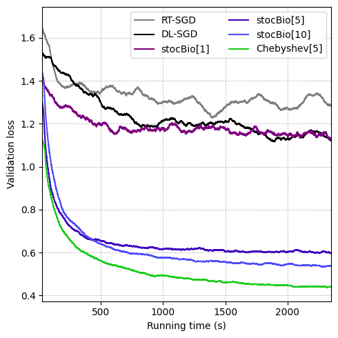
Figure 2: Comparison of various bilevel algorithms on a data cleaning problem with 30% label corruption.

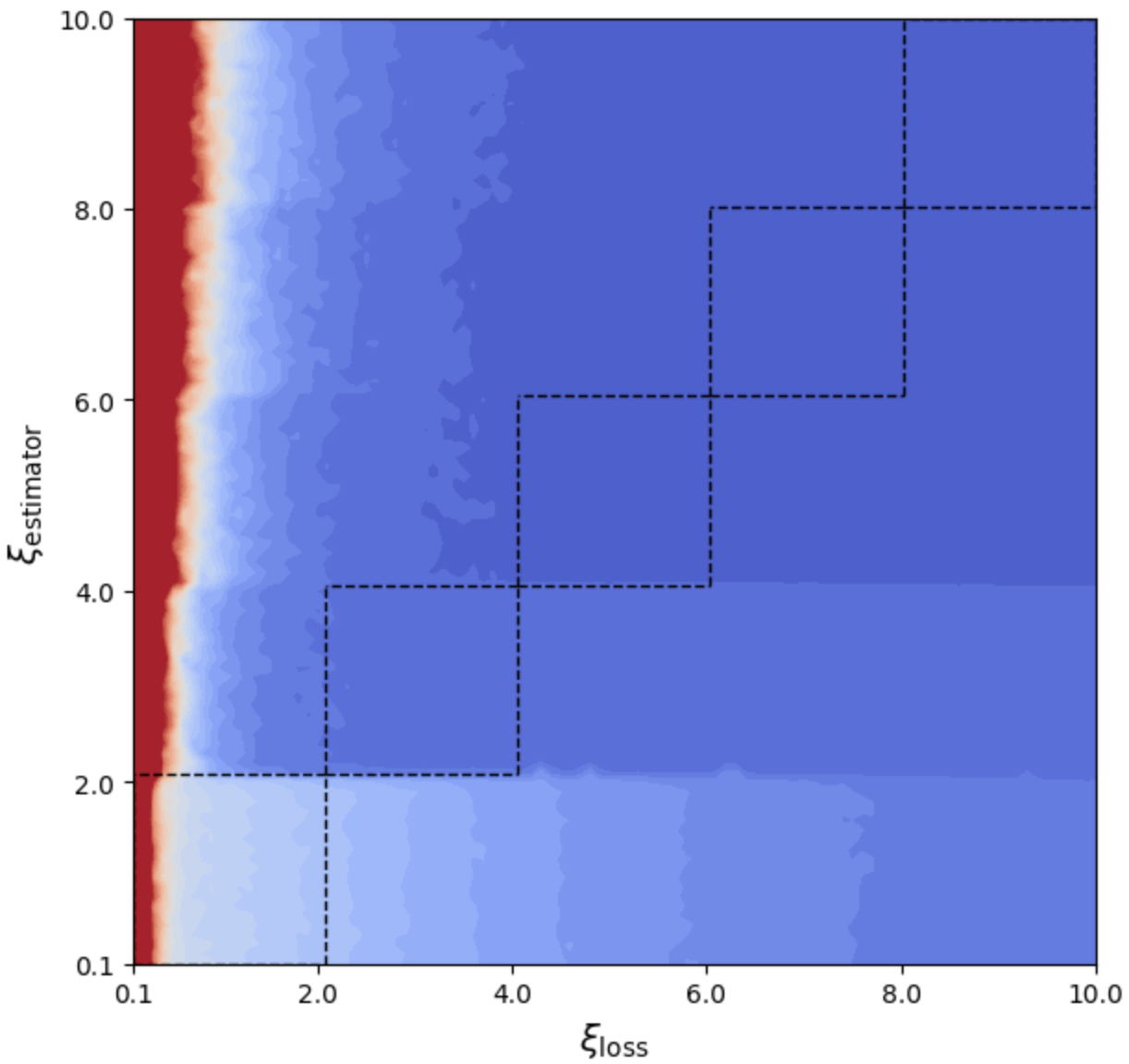
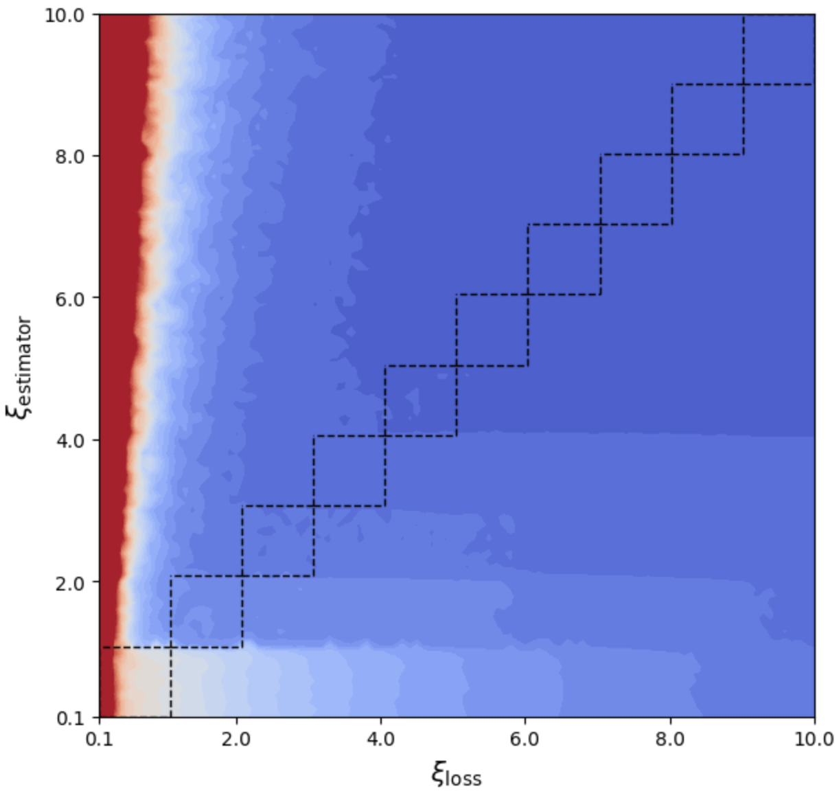
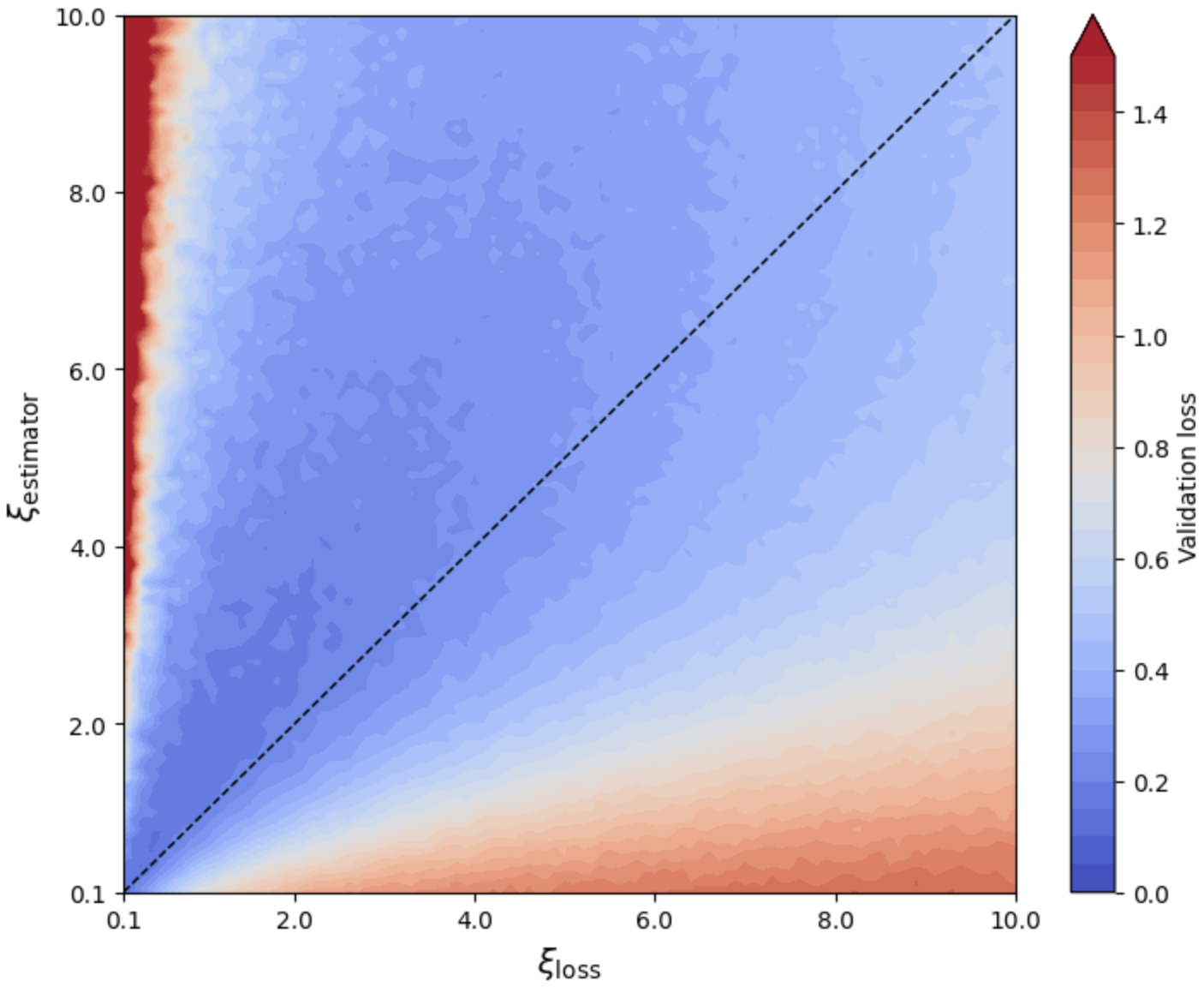
Figure 3: Validation loss of stocBio[5] (left), stocBio[10] (center), and Chebyshev[5] (right) across different tasks temperatures and lower level solutions. Dashed lines delineate the coverage of lower-level solutions.

We compare our proposed reduction framework with stocBio (Ji et al., 2021), and DL-SGD and RT-SGD presented in (Hu et al., 2023b). For stocBio[k], we divide the context space into $k$ equally sized intervals and use one lower level per interval. Note that DL-SGD and RT-SGD do not maintain a finite number of lower level solutions, but instead compute an estimate of $y^{\star}(x,\xi)$ for each $\xi$, starting from a reference point $y_{0}(x)$. Our method, denoted Chebyshev[k], uses the feature map $\Phi$ encoding the first $k$ Chebyshev polynomials, and stocBio[1] as a backbone to solve the SBO reformulation.

It can be seen in Figure 2 that our proposed framework achieves both the fastest convergence rate and best final loss among all competing algorithms. It is worth noting that stocBio[5] and Chebyshev[5] have the same memory usage, while stocBio[10] requires twice as much. SBO algorithms with a single lower level (stocBio[1]) or single reference point (DL-SGD, RT-SGD) maintain a large and noisy validation loss throughout training. This is because the optimal solution $y^{\star}(x,\xi)$ varies significantly with the temperature $\xi$, so that their unique lower level solution or reference point $y_{0}(x)$ is constantly moving toward different solutions $y^{\star}(x,\xi)$. The large variance of RT-SGD makes this phenomenon even more pronounced.

We then investigate the validation loss of each algorithm for different temperatures and their corresponding lower-level solutions. Figure 3 highlights that stocBio[5] and stocBio[10] perform well for large temperatures, as the optimal estimators vary slowly with $\xi$ in this region. However, both suffer from large losses at low temperatures, where $y^{\star}$ varies rapidly. With expert knowledge, one would partition $\Xi$ differently so that lower level solutions are better aligned for low temperatures. The flexibility of Chebyshev[5] enables it to better approximate $y^{\star}$ at low temperatures, allowing it to significantly decrease the validation loss in this range of temperatures, at the cost of slightly lower precision and higher validation loss at high temperatures. This results in a lower overall validation loss across all temperatures.

7 Conclusion

In this work, we addressed the significant challenges of Contextual Stochastic Bilevel Optimization (CSBO) by introducing a novel reduction framework that reformulates CSBO problems into equivalent Stochastic Bilevel Optimization (SBO) problems. This reformulation exploits the parameterization of the lower-level solution using expressive feature maps, such as multivariate Chebyshev polynomials, to decouple the dependency of the lower-level solution on the upper-level decision and context.

Our theoretical analysis established that under standard regularity assumptions, the sample complexity of our proposed framework depends the chosen feature map and its interaction with the context distribution. When both the magnitude and the conditioning of the feature map are controlled, our framework gives a sample complexity for CSBO that is an order of magnitude lower than that of state-of-the-art CSBO algorithms, and matches the lower bound of sample complexity for nonconvex stochastic optimization up to a logarithmic factor. Importantly, this is achieved without the need for impractical conditional sampling oracles. Under additional regularity assumptions, the use of multivariate Chebyshev polynomials as feature map ensures enough expressiveness while maintaining controlled magnitude and conditioning as $\epsilon$ decreases, therefore attaining the near-optimal sample complexity $\tilde{\mathcal{O}}(\epsilon^{-3})$.

We demonstrated the practical benefits of our approach through numerical experiments in hyper-parameter optimization, showing improved convergence rates, reduced validation loss, and enhanced robustness compared to existing methods. The proposed framework effectively balances flexibility and accuracy, enabling superior performance in a range of different contexts.

Overall, our work bridges the complexity gap between CSBO and SBO, offering a practical and efficient solution framework with both strong theoretical guarantees and empirical performance. Future research includes extending this framework to other challenging bi-level or multi-level optimization problems, and dynamic feature maps.

Appendix A Similarity of hypergradients

We first prove Proposition 5.1.

Proof.

Let $x\in\mathbb{R}^{d_{x}}$. Recall that $\nabla F(x)=\mathbb{E}_{(\xi,\eta)}\left[\nabla F(x,\xi,\eta)\right]$ and $\nabla F_{\Phi}(x)=\mathbb{E}_{(\xi,\eta)}\left[\nabla F_{\Phi}(x,\xi,\eta)\right]$ where:

$$\nabla F(x,\xi,\eta) \triangleq\nabla_{1}f(x,y^{\star}(x,\xi),\xi,\eta)\!-\!\nabla_{12}g(x,y^{\star}(x,\xi),\xi,\eta)\left[\nabla_{22}^{2}g(x,y^{\star}(x,\xi),\xi,\eta)\right]^{-1}\nabla_{2}f(x,y^{\star}(x,\xi),\xi,\eta)$$

$$\nabla F_{\Phi}(x,\xi,\eta) \triangleq\nabla_{1}f(x,y_{\Phi}(W^{\star}(x),\xi),\xi,\eta)\!-\!\nabla_{12}g(x,y_{\Phi}(W^{\star}(x),\xi),\xi,\eta)\left[\nabla_{22}^{2}g(x,y_{\Phi}(W^{\star}(x),\xi),\xi,\eta)\right]^{-1}\nabla_{2}f(x,y_{\Phi}(W^{\star}(x),\xi),\xi,\eta)$$

Consider a sample $(\xi,\eta)$. For readability, we define $\Delta_{y}(x,\xi)\triangleq\|y_{\Phi}(W^{\star}(x),\xi)-y^{\star}(x,\xi)\|$ and:

$$A(y_{\Phi}) =\nabla_{12}g(x,y_{\Phi}(W^{\star}(x),\xi),\xi,\eta)\quad\quad A(y^{\star})=\nabla_{12}g(x,y^{\star}(x,\xi),\xi,\eta)$$

$$B(y_{\Phi}) =\nabla_{22}^{2}g(x,y_{\Phi}(W^{\star}(x),\xi),\xi,\eta) B(y^{\star})=\nabla_{22}^{2}g(x,y^{\star}(x,\xi),\xi,\eta)$$

$$C(y_{\Phi}) =\nabla_{2}f(x,y_{\Phi}(W^{\star}(x),\xi),\xi,\eta) C(y^{\star})=\nabla_{2}f(x,y^{\star}(x,\xi),\xi,\eta)$$

We can then write and bound $\|\nabla F_{\Phi}(x,\xi,\eta)-\nabla F(x,\xi,\eta)\|$ using the triangular inequality as:

$$\|\nabla F_{\Phi}(x,\xi,\eta)-\nabla F(x,\xi,\eta)\| \leq\|\nabla_{1}f(x,y_{\Phi}(W^{\star}(x),\xi),\xi,\eta)-\nabla_{1}f(x,y^{\star}(x,\xi),\xi,\eta)\|$$

$$\quad+\|A(y_{\Phi})B(y_{\Phi})^{-1}C(y_{\Phi})-A(y^{\star})B(y^{\star})^{-1}C(y^{\star})\|$$

$$\leq L_{f,1}\Delta_{y}(x,\xi)+\|A(y_{\Phi})-A(y^{\star})\|\cdot\|B(y^{\star})^{-1}\|\cdot\|C(y^{\star})\|$$

$$\quad+\|B(y_{\Phi})^{-1}-B(y^{\star})^{-1}\|\cdot\|A(y_{\Phi})\|\cdot\|C(y_{\Phi})\|+\|C(y_{\Phi})-C(y^{\star})\|\cdot\|A(y_{\Phi})\|\cdot\|B(y^{\star})^{-1}\|$$

From the regularity of $f$, $g$, and their gradient given in Assumption 3.2, we obtain:

$$\|A(y_{\Phi})-A(y^{\star})\| \leq L_{g,2}\Delta_{y}(x,\xi)$$

$$\|B(y_{\Phi})^{-1}-B(y^{\star})^{-1}\| \leq\|B(y_{\Phi})^{-1}\|\cdot\|B(y_{\Phi})-B(y^{\star})\|\cdot\|B(y^{\star})^{-1}\|\leq\frac{L_{g,2}}{\mu^{2}}\Delta_{y}(x,\xi)$$

$$\|C(y_{\Phi})-C(y^{\star})\| \leq L_{f,1}\Delta_{y}(x,\xi)$$

$$\|A(y_{\Phi})\| \leq L_{g,1},$$

$$\|A(y^{\star})\| \leq L_{g,1},$$

$$\|C(y_{\Phi})\| \leq L_{f,0},$$

$$\|C(y^{\star})\| \leq L_{f,0},$$

where the second inequality uses the identity $\|X^{-1}-Y^{-1}\|\leq\|X^{-1}\|\cdot\|X-Y\|\cdot\|Y^{-1}\|$ and the fact that $\|B(y_{\Phi})^{-1}\|$ and $\|B(y^{\star})^{-1}\|$ are upper bounded by $1/\mu$ from the strong convexity of $g$.

It follows that:

$$\|\nabla F_{\Phi}(x,\xi,\eta)-\nabla F(x,\xi,\eta)\| \leq L_{f,1}\Delta_{y}(x,\xi)+\frac{L_{g,2}L_{f,0}}{\mu}\Delta_{y}(x,\xi)+\frac{L_{g,2}L_{g,1}L_{f,0}}{\mu^{2}}\Delta_{y}(x,\xi)+\frac{L_{f,1}L_{g,1}L_{g,2}}{\mu}\Delta_{y}(x,\xi)$$

$$=K\Delta_{y}(x,\xi)$$

where $K=L_{f,1}+\frac{L_{g,2}L_{f,0}}{\mu}+\frac{L_{g,2}L_{g,1}L_{f,0}}{\mu^{2}}+\frac{L_{f,1}L_{g,1}}{\mu}$.

We then bound the difference between the hypergradients using Jensen’s inequality:

$$\|\nabla F_{\Phi}(x)-\nabla F(x)\| \leq\mathbb{E}_{(\xi,\eta)}\|\nabla F_{\Phi}(x,\xi,\eta)-\nabla F(x,\xi,\eta)\|$$

$$\leq K\cdot\mathbb{E}_{(\xi,\eta)}\left[\Delta_{y}(x,\xi)\right]$$

$$=K\cdot\mathbb{E}_{\xi}\|y_{\Phi}(W^{\star}(x),\xi)-y^{\star}(x,\xi)\|$$

∎

We then proceed with the proof of Proposition 5.2.

Proof.

Let $x\in\mathbb{R}^{d_{x}}$, $W\in\mathbb{R}^{d_{y}\times N}$, and $G(x,y,\xi)\triangleq\mathbb{E}_{\eta\sim\mathbb{P}_{\eta|\xi}}\left[g(x,y,\xi,\eta)\right]$. As $g$ is $L_{g,0}$-Lipschitz continuous in $(x,y)$ for any $(\xi,\eta)$, and $\mu$-strongly convex in $y$ for any fixed $(x,\xi,\eta)$, so is $G$. Since $W^{\star}(x)$ minimizes $\mathbb{E}_{\xi}\left[G(x,y_{\Phi}(\cdot,\xi),\xi)\right]$, we have in particular:

$$\mathbb{E}_{\xi}\left[G(x,y_{\Phi}(W^{\star}(x),\xi),\xi)\right]\leq\mathbb{E}_{\xi}\left[G(x,y_{\Phi}(W,\xi),\xi)\right]$$ (3)

Additionally, since $y^{\star}(x,\xi)$ minimizes $G(x,\cdot,\xi)$, it also holds that:

$$G(x,y^{\star}(x,\xi),\xi)\leq G(x,y_{\Phi}(W^{\star}(x),\xi),\xi)$$

Using the strong convexity of $G$ at $W^{\star}(x)$ we thus obtain:

$$G(x,y_{\Phi}(W^{\star}(x),\xi),\xi)-G(x,y^{\star}(x,\xi),\xi)\geq\frac{\mu}{2}\|y_{\Phi}(W^{\star}(x),\xi)-y^{\star}(x,\xi)\|^{2},\quad\forall\xi\in\Xi$$ (4)

On the other hand, the Lipshchitz continuity of $G$ yields:

$$\left|G(x,y_{\Phi}(W,\xi),\xi)-G(x,y^{\star}(x,\xi),\xi)\right|\leq L_{g,0}\|y_{\Phi}(W,\xi)-y^{\star}(x,\xi)\|,\quad\forall\xi\in\Xi$$ (5)

Taking the expectation over $\xi$ on both sides in (4) and (5), and using the inequality (3) we have:

$$\mathbb{E}_{\xi}\|y_{\Phi}(W^{\star}(x),\xi)-y^{\star}(x,\xi)\|^{2} \leq\frac{2}{\mu}\mathbb{E}_{\xi}\left[G(x,y_{\Phi}(W^{\star}(x),\xi),\xi)-G(x,y^{\star}(x,\xi),\xi)\right]$$

$$\leq\frac{2}{\mu}\mathbb{E}_{\xi}\left[G(x,y_{\Phi}(W,\xi),\xi)-G(x,y^{\star}(x,\xi),\xi)\right]$$

$$\leq\frac{2L_{g,0}}{\mu}\mathbb{E}_{\xi}\|y_{\Phi}(W,\xi)-y^{\star}(x,\xi)\|$$

As this holds for any $x\in\mathbb{R}^{d_{x}}$, we obtain the desired result. ∎

Appendix B Regularity of ($\text{SBO}_{\Phi}$)

For readability, we refer in this section to $M_{\Phi}(\epsilon)$ as $M_{\Phi}$, and to $m_{\Phi}(\epsilon)$ as $m_{\Phi}$.

Lemma B.1.

If $A\succeq\mu I_{d_{A}}$ and $B\succeq 0$ with $\mu\geq 0$, then $A\otimes B\succeq\mu I_{d_{A}}\otimes B$ and $B\otimes A\succeq\mu B\otimes I_{d_{A}}$.

Proof.

By the bilinearity of the Kronecker product we have:

$$A\otimes B-\mu I_{d_{A}}\otimes B=(A-\mu I_{d_{A}})\otimes B$$

Since the Kronecker product of two positive definite matrix is positive definite, it holds that $(A-\mu I_{d_{A}})\otimes B\succeq 0$ and thus $A\otimes B-\mu A\otimes I_{d_{B}}\succeq 0$. With a symmetrical argument, we obtain $B\otimes A\succeq\mu B\otimes I_{d_{A}}$. ∎

B.1 Lipschitz continuity

Lemma B.2.

Let $h(x,y,\xi,\eta):\mathbb{R}^{d_{x}}\times\mathbb{R}^{d_{y}}\times\Xi\times\mathbb{R}^{d_{\eta}}\to\mathbb{R}^{n}$ and $l(\xi):\Xi\to\mathbb{R}^{N}$. Suppose the following conditions hold:

1. $h$ is $L$-Lipschitz continuous with respect to $(x,y)$ for any fixed $(\xi,\eta)$.

2. There exists a constant $M$ such that:

   $$\|l(\xi)\|\leq M,\quad\forall\xi\in\Xi$$

Then the mapping $h_{\Phi}:(x,W,\xi,\eta)\mapsto h(x,W\Phi(\xi),\xi,\eta)l(\xi)$ is $LM_{\Phi}M$-Lipschitz continuous with respect to $(x,y)$ for all fixed $(\xi,\eta)$.

Proof.

Since $h(x,y,\xi,\eta)$ is $L$-Lipschitz continuous in $(x,y)$ and $\sup_{\xi\in\Xi}||\Phi(\xi)||\leq M_{\Phi}$, we have for any $(x,W)$ and $(x^{\prime},W^{\prime})$:

$$\left\|h_{\Phi}(x,W,\xi,\eta)-h_{\Phi}(x^{\prime},W^{\prime},\xi,\eta)\right\| =\left\|h(x,W\Phi(\xi),\xi,\eta)l(\xi)-h(x^{\prime},W^{\prime}\Phi(\xi),\xi,\eta)l(\xi)\right\|$$

$$\stackrel{{\scriptstyle\scriptscriptstyle(\mkern-1.5mu1\mkern-1.5mu)}}{{\leq}}\left\|h(x,W\Phi(\xi),\xi,\eta)-h(x^{\prime},W^{\prime}\Phi(\xi),\xi,\eta)\right\|\cdot\|l(\xi)\|$$

$$\stackrel{{\scriptstyle\scriptscriptstyle(\mkern-1.5mu2\mkern-1.5mu)}}{{\leq}}ML\left(\|x-x^{\prime}\|+\|W\Phi(\xi)-W^{\prime}\Phi(\xi)\|\right)$$

$$\stackrel{{\scriptstyle\scriptscriptstyle(\mkern-1.5mu3\mkern-1.5mu)}}{{\leq}}ML\left(\|x-x^{\prime}\|+M_{\Phi}\|W-W^{\prime}\|\right)$$

$$\stackrel{{\scriptstyle\scriptscriptstyle(\mkern-1.5mu4\mkern-1.5mu)}}{{\leq}}LM_{\Phi}M\left(\|x-x^{\prime}\|+\|W-W^{\prime}\|\right)$$

where (1) uses the sub-multiplicativity of $\|\cdot\|$, (2) follows from the Lipschitz continuity of $h$ and this inequality $\|l(\xi)\|\leq M$, (3) uses again the sub-multiplicativity of $\|\cdot\|$ and the inequality $\|\Phi(\xi)\|\leq M_{\Phi}(\epsilon)$, and (4) holds since $1\leq M_{\Phi}$. Therefore $h_{\Phi}$ is $LM_{\Phi}M$-Lipschitz continuous in $(x,W)$. ∎

Lemma B.3.

The following hold under assumption 3.2:

1. The functions $f_{\Phi}(x,W,\xi,\eta)$ and $g_{\Phi}(x,W,\xi,\eta)$ are $L_{f,0}M_{\Phi}$ and $L_{g,0}M_{\Phi}$-Lipschitz, respectively, with respect to $x$ and $W$.

2. The gradients $\nabla f_{\Phi}(x,W,\xi,\eta)$ and $\nabla g_{\Phi}(x,W,\xi,\eta)$ are $L_{f,1}M_{\Phi}^{2}$ and $L_{g,1}M_{\Phi}^{2}$-Lipschitz, respectively, with respect to $x$ and $W$.

3. The second order gradients $\nabla_{12}^{2}g_{\Phi}(x,W,\xi,\eta)$ and $\nabla_{22}^{2}g_{\Phi}(x,W,\xi,\eta)$ are $L_{g,2}M_{\Phi}^{3}$-Lipschitz with respect to $x$ and $W$.

Proof.

Under assumption 3.2-(i), the mappings $f$, $g$, $\nabla f$, $\nabla g$, and $\nabla^{2}g$, are $L_{f,0}$, $L_{g,0}$, $L_{f,1}$, $L_{g,1}$, and $L_{g,2}$- Lipschitz continuous with respect to $(x,y)$ for any fixed $(\xi,\eta)$, respectively. Additionally, the chain rule gives:

$$\nabla_{1}f_{\Phi}(x,W,\xi,\eta) =\nabla_{1}f(x,W\Phi(\xi),\xi,\eta)$$

$$\nabla_{2}f_{\Phi}(x,W,\xi,\eta) =\nabla_{2}f(x,W\Phi(\xi),\xi,\eta)\Phi(\xi)^{\top}$$

$$\nabla_{1}g_{\Phi}(x,W,\xi,\eta) =\nabla_{1}g(x,W\Phi(\xi),\xi,\eta)$$

$$\nabla_{2}g_{\Phi}(x,W,\xi,\eta) =\nabla_{2}g(x,W\Phi(\xi),\xi,\eta)\Phi(\xi)^{\top}$$

$$\nabla_{12}^{2}g_{\Phi}(x,W,\xi,\eta) =\nabla_{12}^{2}g(x,W\Phi(\xi),\xi,\eta)\Phi(\xi)^{\top}$$

$$\nabla_{22}^{2}g_{\Phi}(x,W,\xi,\eta) =\nabla_{22}^{2}g(x,W\Phi(\xi),\xi,\eta)\otimes\Phi(\xi)\Phi(\xi)^{\top}$$

We can then use Lemma B.2 to obtain the following:

$h$	$l$	$L$	$M$	Lipschitz coefficient of $h(x,W\Phi(\xi),\xi,\eta)$ w.r.t. $(x,W)$
$f_{\Phi}$	$1$	$L_{f,0}$	$1$	$L_{f,0}M_{\Phi}$
$g_{\Phi}$	$1$	$L_{g,0}$	$1$	$L_{g,0}M_{\Phi}$
$\nabla_{1}f_{\Phi}$	$I_{d_{x}}$	$L_{f,1}$	$1$	$L_{f,1}M_{\Phi}$
$\nabla_{2}f_{\Phi}$	$\Phi^{\top}$	$L_{f,1}$	$M_{\Phi}$	$L_{f,1}M_{\Phi}^{2}$
$\nabla_{1}g_{\Phi}$	$I_{d_{x}}$	$L_{g,1}$	$1$	$L_{g,1}M_{\Phi}$
$\nabla_{2}g_{\Phi}$	$\Phi^{\top}$	$L_{g,1}$	$M_{\Phi}$	$L_{g,1}M_{\Phi}^{2}$
$\nabla_{12}^{2}g_{\Phi}$	$\Phi^{\top}$	$L_{g,2}$	$M_{\Phi}$	$L_{g,2}M_{\Phi}^{2}$
$\nabla_{22}^{2}g_{\Phi}$	$\Phi\Phi^{\top}$	$L_{g,2}$	$M_{\Phi}^{2}$	$L_{g,2}M_{\Phi}^{3}$

and we conclude using the inequality $1\leq M_{\Phi}$. ∎

B.2 Bounded variance

Lemma B.4.

Let $h(x,y,\xi,\eta):\mathbb{R}^{d_{x}}\times\mathbb{R}^{d_{y}}\times\Xi\times\mathbb{R}^{d_{\eta}}\to\mathbb{R}^{n}$ and $\l (\xi):\Xi\to\mathbb{R}^{N}$. Suppose the following conditions hold:

1. $h(x,y,\xi,\eta)$ has, conditioned on $\xi$, a variance bounded by $\sigma^{2}$ i.e.

   $$\mathbb{E}_{\eta\sim\mathbb{P}_{\eta|\xi}}\left\|h(x,y,\xi,\eta)-\mathbb{E}_{\eta^{\prime}\sim\mathbb{P}_{\eta|\xi}}\left[h(x,y,\xi,\eta^{\prime})\right]\right\|^{2}\leq\sigma^{2},\quad\forall x\in\mathbb{R}^{d_{x}},y\in\mathbb{R}^{d_{y}},\xi\in\mathbb{R}^{d_{\xi}}.$$

2. There exists a constant $C$ such that:

   $$\mathbb{E}_{\eta\sim\mathbb{P}_{\eta|\xi}}\left\|h(x,y,\xi,\eta)\right\|\leq C,\quad\forall x\in\mathbb{R}^{d_{x}},y\in\mathbb{R}^{d_{y}},\xi\in\mathbb{R}^{d_{\xi}}$$

3. There exists a constant $M$ such that:

   $$\|l(\xi)\|\leq M,\quad\forall\xi\in\Xi$$

Then the mapping $h_{\Phi}:(x,W,\xi,\eta)\mapsto h(x,W\Phi(\xi),\xi,\eta)l(\xi)$ has a variance bounded by $M^{2}\left(\sigma^{2}+C^{2}\right)$.

Proof.

Let $Z=h_{\Phi}(x,W,\xi,\eta)$. Using the law of total variance we have:

$$\text{Var}_{(\xi,\eta)}\left[Z\right]=\mathbb{E}_{\xi}\left[\text{Var}_{\eta|\xi}\left[Z\;|\;\xi\right]\right]+\text{Var}_{\xi}\left[\mathbb{E}_{\eta|\xi}\left[Z\;|\;\xi\right]\right]$$

For all $\xi\in\Xi$ it holds that:

$$\text{Var}_{\eta|\xi}\left[Z\;|\;\xi\right] =\mathbb{E}_{\eta|\xi}\left[\left\|h(x,W\Phi(\xi),\xi,\eta)l(\xi)-\mathbb{E}_{\eta^{\prime}|\xi}\left[h(x,W\Phi(\xi),\xi,\eta^{\prime})l(\xi)\right]\right\|^{2}\bigg{|}\xi\right]$$

$$\leq\|l(\xi)\|^{2}\cdot\mathbb{E}_{\eta|\xi}\left[\left\|h(x,W\Phi(\xi),\xi,\eta)-\mathbb{E}_{\eta^{\prime}|\xi}\left[h(x,W\Phi(\xi),\xi,\eta^{\prime})\right]\right\|^{2}\bigg{|}\xi\right]$$

$$\leq\|l(\xi)\|^{2}\cdot\sigma^{2}$$

where the second inequality follows from the sub-multiplicativity of $\|\cdot\|$ and the fact that $l(\xi)$ is deterministic when conditioned on $\xi$, and the last inequality holds under condition 1.

Similarly, we have that for all $\xi\in\Xi$ and under condition 2:

$$\left\|\mathbb{E}_{\eta|\xi}\left[Z\;|\;\xi\right]\right\| \leq\left\|\mathbb{E}\left[h_{\Phi}(x,W,\xi,\eta)l(\xi)\;|\;\xi\right]\right\|$$

$$\leq\|l(\xi)\|\cdot\left\|\mathbb{E}\left[h_{\Phi}(x,W,\xi,\eta)\;|\;\xi\right]\right\|$$

$$\leq\|l(\xi)\|\cdot C$$

Combining the above results, we obtain:

$$\text{Var}_{(\xi,\eta)}\left[Z\right] \leq\mathbb{E}_{\xi}\left[\|l(\xi)\|^{2}\sigma^{2}\right]+\mathbb{E}_{\xi}\left[\left\|\mathbb{E}_{\eta|\xi}\left[Z\;|\;\xi\right]\right\|^{2}\right]$$

$$\leq M^{2}\sigma^{2}+\mathbb{E}_{\xi}\left[\|l(\xi)\|^{2}\cdot C^{2}\right]$$

$$\leq M^{2}\left(\sigma^{2}+C^{2}\right)$$

where the last inequality uses condition 3. ∎

Lemma B.5.

Under assumption 3.2, the mappings $\nabla_{1}f_{\Phi}(x,W,\xi,\eta)$, $\nabla_{2}f_{\Phi}(x,W,\xi,\eta)$, $\nabla_{1}g_{\Phi}(x,W,\xi,\eta)$, $\nabla_{12}^{2}g_{\Phi}(x,W,\xi,\eta)$, and $\nabla_{22}^{2}g_{\Phi}(x,W,\xi,\eta)$ have a bounded variance.

Proof.

Under assumption 3.2-(iii) we have for any $(x,W,\xi)$ that the variances of $\nabla_{1}f_{\Phi}(x,W,\xi,\eta)$ and $\nabla_{2}f_{\Phi}(x,W,\xi,\eta)$ are upper bounded by $\sigma^{2}_{f}$, the variance of $\nabla_{1}g_{\Phi}(x,W,\xi,\eta)$ by $\sigma^{2}_{g,1}$, and the variance of $\nabla_{12}^{2}g_{\Phi}(x,W,\xi,\eta)$ and $\nabla_{22}^{2}g_{\Phi}(x,W,\xi,\eta)$ by $\sigma^{2}_{g,2}$. Thus all 5 functions considered satisfy the first condition of Lemma B.5. From the Lipschitz continuity of $f$, $g$ and their gradients (assumption 3.2-(i)) we have for any $(x,y,\xi,\eta)$:

$$\left\|\nabla_{1}f(x,y,\xi,\eta)\right\| \leq L_{f,0}$$

$$\left\|\nabla_{2}f(x,y,\xi,\eta)\right\| \leq L_{f,0}$$

$$\left\|\nabla_{2}g(x,y,\xi,\eta)\right\| \leq L_{g,0}$$

$$\left\|\nabla_{12}^{2}g(x,y,\xi,\eta)\right\| \leq L_{g,1}$$

$$\left\|\nabla_{22}^{2}g(x,y,\xi,\eta)\right\| \leq L_{g,1}$$

Taking the expectation over $\eta\sim\mathbb{P}_{\eta|\xi}$, the second condition of Lemma B.5 holds for all 5 functions considered. We then use the chain rule to get:

$$\nabla_{1}f_{\Phi}(x,W,\xi,\eta) =\nabla_{1}f(x,W\Phi(\xi),\xi,\eta)$$

$$\nabla_{2}f_{\Phi}(x,W,\xi,\eta) =\nabla_{2}f(x,W\Phi(\xi),\xi,\eta)\Phi(\xi)^{\top}$$

$$\nabla_{2}g_{\Phi}(x,W,\xi,\eta) =\nabla_{2}g(x,W\Phi(\xi),\xi,\eta)\Phi(\xi)^{\top}$$

$$\nabla_{12}^{2}g_{\Phi}(x,W,\xi,\eta) =\nabla_{12}^{2}g(x,W\Phi(\xi),\xi,\eta)\Phi(\xi)^{\top}$$

$$\nabla_{22}^{2}g_{\Phi}(x,W,\xi,\eta) =\nabla_{22}^{2}g(x,W\Phi(\xi),\xi,\eta)\otimes\Phi(\xi)\Phi(\xi)^{\top}$$

Since $\|\Phi(\xi)\|\leq M_{\Phi}$, Lemma B.4 applies and we obtain the following bounds:

$h$	$l$	$C$	$M$	Bound on $\text{Var}_{(\xi,\eta)}\left[h_{\Phi}(x,W,\xi,\eta)\right]$
$\nabla_{1}f_{\Phi}$	$I_{d_{x}}$	$L_{f,0}$	$1$	$\sigma_{f}^{2}+L_{f,0}^{2}$
$\nabla_{2}f_{\Phi}$	$\Phi^{\top}$	$L_{f,0}$	$M_{\Phi}$	$M_{\Phi}^{2}\left(\sigma_{f}^{2}+L_{f,0}^{2}\right)$
$\nabla_{2}g_{\Phi}$	$\Phi^{\top}$	$L_{g,0}$	$M_{\Phi}$	$M_{\Phi}^{2}\left(\sigma_{g,1}^{2}+L_{g,0}^{2}\right)$
$\nabla_{12}^{2}g_{\Phi}$	$\Phi^{\top}$	$L_{g,1}$	$M_{\Phi}$	$M_{\Phi}^{2}\left(\sigma_{g,2}^{2}+L_{g,1}^{2}\right)$
$\nabla_{22}^{2}g_{\Phi}$	$\Phi\Phi^{\top}$	$L_{g,1}$	$M_{\Phi}^{2}$	$M_{\Phi}^{4}\left(\sigma_{g,2}^{2}+L_{g,1}^{2}\right)$

We conclude that all 5 mappings have a bounded variance. ∎

B.3 Strong convexity of $G_{\Phi}(x,W)\triangleq\mathbb{E}_{(\xi,\eta)}\left[g(x,W\Phi(\xi),\xi,\eta)\right]$

Lemma B.6.

Under assumptions 3.2-(ii) and if $\Phi$ is well-conditioned, $G_{\Phi}$ is $\mu m_{\Phi}(\epsilon)$-strongly convex in $W$ for any fixed $x\in\mathbb{R}^{d_{x}}$.

Proof.

We have for any fixed $x\in\mathbb{R}^{d_{x}}$ that $G_{\Phi}$ is twice differentiable with respect to $W$ as the expectation of compositions of twice differentiable and linear mapping. Additionally:

$$\nabla_{22}^{2}G_{\Phi}(x,W) =\mathbb{E}_{\xi}\left[\nabla_{22}^{2}G(x,W\Phi(\xi),\xi)\otimes\Phi(\xi)\Phi(\xi)^{\top}\right]$$

Since $G$ is $\mu$-strongly convexity with respect to $y$ with $\mu>0$ and $\mathbb{E}_{\xi}\left[\Phi(\xi)\Phi(\xi)^{\top}\right]\succeq m_{\Phi}(\epsilon)I_{N_{\Phi}(\epsilon)}\succeq 0$, we obtain using Lemma B.1 twice:

$$\nabla_{22}^{2}G_{\Phi}(x,W) \succeq\mu\mathbb{E}_{\xi}\left[I_{d_{y}}\otimes\Phi(\xi)\Phi(\xi)^{\top}\right]$$

$$=\mu I_{d_{y}}\otimes\mathbb{E}_{\xi}\left[\Phi(\xi)\Phi(\xi)^{\top}\right]$$

$$\succeq\mu m_{\Phi}(\epsilon)I_{d_{y}}\otimes I_{N_{\Phi}(\epsilon)}$$

$$=\mu m_{\Phi}(\epsilon)I_{d_{y}\cdot N_{\Phi}(\epsilon)}$$

and we conclude that $G_{\Phi}(x,W)$ is $\mu m_{\Phi}(\epsilon)$-strongly convex with respect to $W$ for any $x\in\mathbb{R}_{d_{x}}$. ∎

Appendix C Proof of Theorem 4.5

In this proof, we use the notations $\lesssim$, $\simeq$, and $\gtrsim$ to denote relations up to a constant. We will show that under assumptions 3.2 and if $\Phi$ is well-conditioned, the assumptions 1 and 2 of (Guo et al., 2021) hold for $f_{\Phi}$ and $g_{\Phi}$. Namely, we want to show:

Assumption C.1.

For any $x\in\mathbb{R}^{d_{x}}$, $\mathbb{E}_{(\xi,\eta)}\left[g_{\Phi}\left(x,W,\xi,\eta\right)\right]$ is $\lambda$-strongly convex and $L$-smooth.

and

Assumption C.2.

The following hold:

1. $\nabla_{1}f_{\Phi}$ is $L_{fx}$-Lipschitz continuous, $\nabla_{2}f_{\Phi}$ is $L_{fy}$-Lipschitz continuous, $\nabla_{2}g_{\Phi}$ is $L_{gy}$-Lipschitz continuous, $\nabla_{12}^{2}f_{\Phi}$ is $L_{gxy}$-Lipschitz continuous, $\nabla_{22}^{2}f_{\Phi}$ is $L_{gyy}$-Lipschitz continuous, all with respect to $(x,W)$.

2. $\nabla_{1}f_{\Phi}$, $\nabla_{2}f_{\Phi}$, $\nabla_{2}g_{\Phi}$, $\nabla_{12}^{2}f_{\Phi}$, and $\nabla_{22}^{2}f_{\Phi}$ have a variance bounded by $\sigma^{2}$.

3. $\|\nabla_{2}\mathbb{E}_{(\xi,\eta)}\left[f(x,W,\xi,\eta)\right]\|^{2}\leq C_{fy}^{2}$, $\|\nabla_{12}^{2}\mathbb{E}_{(\xi,\eta)}\left[g(x,W,\xi,\eta)\right]\|^{2}\leq C_{gxy}^{2}$.

Under assumption 3.2 and if $\Phi$ is well-conditioned, Lemma B.6 gives $\mathbb{E}_{(\xi,\eta)}\left[g_{\Phi}\left(x,W,\xi,\eta\right)\right]$ is $\mu m_{\Phi}(\epsilon)$-strongly convex with respect to $W$ for any $x\in\mathbb{R}^{d_{x}}$. Further, we have from Lemma B.3 that $\nabla_{2}g_{\Phi}\left(x,W,\xi,\eta\right)$ is $L_{g,1}M_{\Phi}^{2}$-Lipchitz continuous in $W$ for all fixed $(x,\xi,\eta)$. Taking the expectation over $(\xi,\eta)$ we obtain:

$$\left\|\nabla_{2}\mathbb{E}_{(\xi,\eta)}\left[g_{\Phi}\left(x,W,\xi,\eta\right)\right]-\nabla_{2}\mathbb{E}_{(\xi,\eta)}\left[g_{\Phi}\left(x^{\prime},W^{\prime},\xi,\eta\right)\right]\right\| =\left\|\mathbb{E}_{(\xi,\eta)}\left[\nabla_{2}g_{\Phi}\left(x,W,\xi,\eta\right)-\nabla_{2}g_{\Phi}\left(x^{\prime},W^{\prime},\xi,\eta\right)\right]\right\|$$

$$\leq\mathbb{E}_{(\xi,\eta)}\left[\left\|\nabla_{2}g_{\Phi}\left(x,W,\xi,\eta\right)-\nabla_{2}g_{\Phi}\left(x^{\prime},W^{\prime},\xi,\eta\right)\right\|\right]$$

$$\leq L_{g,1}M_{\Phi}^{2}\left(\|x-x^{\prime}\|+\|W-W^{\prime}\|\right)$$

where the first inequality holds since assumption 3.2 implies that $\nabla_{2}g_{\Phi}\left(x,W,\xi,\eta\right)$ is unbiased and the second inequality uses Jensen’s inequality. Therefore $\mathbb{E}_{(\xi,\eta)}\left[g_{\Phi}\left(x,W,\xi,\eta\right)\right]$ is $L_{g,1}M_{\Phi}^{2}$-smooth for any fixed $x\in\mathbb{R}^{d_{x}}$ and assumption C.1 holds with $\lambda=\mu m_{\Phi}(\epsilon)$ and $L=L_{g,1}M_{\Phi}^{2}$.

Additionally, Lemma B.3 and Lemma B.5 show that assumption $\ref{assumption:Guo_2}-(i)$ and $\ref{assumption:Guo_2}-(ii)$ hold $f_{\Phi}$ and $g_{\Phi}$ for with Lipchitz constant $L$ and uniform variance bound $\sigma^{2}$ given in the table below.

$h$	$L$	$\sigma^{2}$
$\nabla_{1}f_{\Phi}$	$L_{f,1}M_{\Phi}$	$\sigma_{f}^{2}+L_{f,0}^{2}$
$\nabla_{2}f_{\Phi}$	$L_{f,1}M_{\Phi}^{2}$	$M_{\Phi}^{2}\left(\sigma_{f}^{2}+L_{f,0}^{2}\right)$
$\nabla_{2}g_{\Phi}$	$L_{g,1}M_{\Phi}^{2}$	$M_{\Phi}^{2}\left(\sigma_{g,1}^{2}+L_{g,0}^{2}\right)$
$\nabla_{12}^{2}g_{\Phi}$	$L_{g,2}M_{\Phi}^{2}$	$M_{\Phi}^{2}\left(\sigma_{g,2}^{2}+L_{g,1}^{2}\right)$
$\nabla_{22}^{2}g_{\Phi}$	$L_{g,2}M_{\Phi}^{3}$	$M_{\Phi}^{4}\left(\sigma_{g,2}^{2}+L_{g,1}^{2}\right)$

Further, Lemma B.3 also gives that $f_{\Phi}$ and $g_{\phi}$ are $L_{f,0}M_{\Phi}$ and $L_{g,0}M_{\Phi}$-Lipschitz continuous in $(x,W)$, respectively. It follows that that $\|\nabla_{1}\mathbb{E}_{(\xi,\eta)}\left[f_{\Phi}\left(x,W,\xi,\eta\right)\right]\|\leq L_{f,0}M_{\Phi}$ and $\|\nabla_{2}\mathbb{E}_{(\xi,\eta)}\left[g_{\Phi}\left(x,W,\xi,\eta\right)\right]\|\leq L_{g,0}M_{\Phi}$. Hence condition $\ref{assumption:Guo_2}-(iii)$ hold for $f_{\Phi}$ and $g_{\Phi}$ with $C_{fy}=L_{f,0}M_{\Phi}$ and $C_{gxy}=L_{g,1}M_{\Phi}^{2}$.

Therefore Theorem 1 of (Guo et al., 2021) holds. Before stating it we first bound some quantities in term of $M_{\Phi}$ and $m_{\Phi}$.

Since $\Phi$ is well conditioned, we have $\Sigma_{\Phi}\succeq m_{\phi}I_{N_{\Phi}(\epsilon)}$. Therefore:

$$\mathbb{E}_{\xi}\left[\|W^{\star}(x_{0})\Phi(\xi)\|^{2}\right] =\mathbb{E}_{\xi}\left[(W^{\star}(x_{0})\Phi(\xi))^{\top}W^{\star}(x_{0})\Phi(\xi)\right]$$

$$=\mathbb{E}_{\xi}\left[\text{tr}\left(W^{\star}(x_{0})\Phi(\xi)(W^{\star}(x_{0})\Phi(\xi))^{\top}\right)\right]$$

$$=\text{tr}\left(W^{\star}(x_{0})\mathbb{E}_{\xi}\left[\Phi(\xi)\Phi(\xi)^{\top}\right]{W^{\star}(x_{0})}^{\top}\right)$$

$$\geq m_{\phi}\text{tr}\left(W^{\star}(x_{0}){W^{\star}(x_{0})}^{\top}\right)$$

$$=m_{\phi}\|W^{\star}(x_{0})\|^{2}_{F}$$

$$\geq m_{\phi}\|W^{\star}(x_{0})\|^{2}$$

For any $(x_{0},W_{0})$ and by the $\mu$ strong convexity of $g$ we have:

$$\mathbb{E}_{(\xi,\eta)}\left[g_{\Phi}(x_{0},W_{0},\xi,\eta)\right]\geq\mathbb{E}_{(\xi,\eta)}\left[g_{\Phi}(x_{0},W^{\star}(x_{0}),\xi,\eta)\right]+\frac{\mu}{2}\mathbb{E}_{(\xi,\eta)}\left[\|W^{\star}(x_{0})\Phi(\xi)\|^{2}\right]$$

and thus, taking $W_{0}=0$:

$$\mathbb{E}_{\xi}\left[\|W^{\star}(x_{0})\Phi(\xi)\|^{2}\right] \leq\frac{2}{\mu}\mathbb{E}_{(\xi,\eta)}\left[g_{\Phi}(x_{0},W_{0},\xi,\eta)-g_{\Phi}(x_{0},W^{\star}(x_{0}),\xi,\eta)\right]$$

$$\leq\frac{2}{\mu}\underbrace{\left(\mathbb{E}_{(\xi,\eta)}\left[g(x_{0},0,\xi,\eta)-\min_{y}g(x_{0},y,\xi,\eta)\right]\right)}_{\Delta_{g,0}}$$

Combining the above results we obtain:

$$\|W^{\star}(x_{0})\|^{2} \leq\frac{\mathbb{E}_{\xi}\left[\|W^{\star}(x_{0})\Phi(\xi)\|^{2}\right]}{m_{\Phi}}$$

$$\leq\frac{2\Delta_{g,0}}{\mu\cdot m_{\Phi}}$$

From Lemma 2.2 in (Ghadimi & Wang, 2018), $W^{\star}(x)$ is Lipschitz continuous in $x$ with constant $L_{W}=\frac{L_{gy}}{\lambda}=\frac{L_{g,1}M_{\Phi}^{2}}{\mu m_{\Phi}}$. Additionally, $\nabla F$ is Lipschitz continuous in $x$ with constant

$$L_{F} =L_{fy}+\frac{L_{fy}L_{gy}}{\lambda}+\frac{L_{gy}}{\lambda}\left(L_{fy}+\frac{L_{fy}L_{gy}}{\lambda}+L_{f}\left[\frac{L_{gxy}}{\lambda}+\frac{L_{gyy}L_{gy}}{\lambda^{2}}\right]\right)+L_{f}\left[\frac{L_{gxy}L_{f}}{\lambda}+\frac{L_{gyy}L_{gy}}{\lambda^{2}}\right]$$

$$=L_{fy}+\frac{2L_{fy}L_{gy}+L_{f}^{2}L_{gxy}}{\lambda}+\frac{L_{fy}L_{gy}^{2}+L_{f}L_{gy}L_{gxy}+L_{f}L_{gyy}L_{gy}}{\lambda^{2}}+\frac{L_{f}L_{gy}^{2}L_{gyy}}{\lambda^{3}}$$

$$\lesssim M_{\Phi}^{2}+\frac{M_{\Phi}^{5}}{m_{\Phi}}+\frac{M_{\Phi}^{6}}{m_{\Phi}^{2}}+\frac{M_{\Phi}^{8}}{m_{\Phi}^{3}}$$

$$\lesssim\frac{M_{\Phi}^{8}}{m_{\Phi}^{3}}$$

Using the notations of (Guo et al., 2021), we have $\delta_{W,0}\triangleq\|W_{1}-W^{\star}(x_{0})\|^{2}$ with $W_{1}=W_{0}-\tau_{0}\tau w_{1}$ and have:

$$\delta_{fx,0} \lesssim\|\nabla_{1}f_{\Phi}(x_{0},W_{0}))\|^{2}\lesssim M_{\Phi}^{2}$$

$$\delta_{fy,0} \lesssim\|\nabla_{2}f_{\Phi}(x_{0},W_{0}))\|^{2}\lesssim M_{\Phi}^{4}$$

$$\delta_{gy,0} \lesssim\|\nabla_{2}g_{\Phi}(x_{0},W_{0}))\|^{2}\lesssim M_{\Phi}^{4}$$

$$\delta_{gxy,0} \lesssim\|\nabla_{12}g_{\Phi}(x_{0},W_{0}))\|^{2}\lesssim M_{\Phi}^{4}$$

$$\delta_{gyy,0} \lesssim\|\nabla_{22}g_{\Phi}(x_{0},W_{0}))\|^{2}\lesssim M_{\Phi}^{6}$$

Theorem 1 of (Guo et al., 2021) finally give:

$$\frac{1}{2(T+1)}\mathbb{E}\left[\sum_{t=0}^{T}\|\nabla F_{\Phi}(x_{t})\|^{2}\right]\leq\frac{F_{\Phi}(x_{0})-F_{\Phi}(x^{\star})}{\gamma\eta_{T}T}+\frac{C\mathbb{E}\left[\delta_{W,0}\right]}{\eta_{T}T}+\frac{\mathbb{E}\left[\delta_{gy,0}+\delta_{fx,0}+\delta_{fy,0}+\delta_{gxy,0}+\delta_{gyy,0}\right]}{\gamma\eta_{0}\eta_{T}T}+\frac{\mathcal{O}\left(\ln(T+2)\right)}{\gamma\eta_{T}T}$$ (6)

where for $c=1$:

$$C_{0} =\left(2L_{fx}^{2}+\frac{6C_{fy}^{2}L_{gxy}^{2}}{\lambda^{2}}+\frac{6C_{fy}^{2}C_{gxy}^{2}L_{gyy}^{2}}{\lambda^{4}}+\frac{6L_{fy}^{2}C_{gxy}^{2}}{\lambda^{2}}\right)\lesssim\frac{M_{\Phi}^{12}}{m_{\Phi}^{4}}$$

$$C_{1} =2$$

$$C_{2} =\frac{6C_{fy}^{2}}{\lambda^{2}}\simeq\frac{M_{\Phi}^{2}}{m_{\Phi}^{2}}$$

$$C_{3} =\frac{6C_{fy}^{2}C_{gxy}^{2}}{\lambda^{4}}\simeq\frac{M_{\Phi}^{6}}{m_{\Phi}^{4}}$$

$$C_{4} =\frac{6C_{gxy}^{2}}{\lambda^{2}}\simeq\frac{M_{\Phi}^{4}}{m_{\Phi}^{2}}$$

$$\tau =\frac{1}{3L_{g}}\simeq\frac{1}{M_{\Phi}^{2}}$$

$$C =\max\left\{\frac{4C_{0}}{\tau\lambda},\frac{4\left(L_{gy}^{2}+L_{fx}^{2}+L_{fy}^{2}+L_{gxy}^{2}+L_{gyy}^{2}\right)}{\gamma}\right\}\lesssim\frac{M_{\Phi}^{18}}{m_{\Phi}^{5}}$$

$$\gamma =\min\left\{\frac{\sqrt{\tau\lambda}}{8\sqrt{C}L_{W}},\frac{1}{16\left(L_{gy}^{2}+L_{fx}^{2}+L_{fy}^{2}+L_{gxy}^{2}+L_{gyy}^{2}\right)}\right\}\gtrsim\frac{m_{\Phi}^{4}}{M_{\Phi}^{12}}$$

$$c_{0} =\max\left\{2,64L_{F}^{3},\left(\frac{\lambda}{16C\gamma\tau}\right)^{3/2},\left(\frac{2}{7L_{F}}\right)^{3/2},(2(C_{1}+C_{2}+C_{3}+C_{4})\gamma)^{3/2}\right\}\simeq\frac{M_{\Phi}^{24}}{m_{\Phi}^{9}}$$

$$\eta_{t} =\tau_{t}=\frac{1}{(c_{0}+t)^{1/3}}$$

Here the bounds on $C$ and $\gamma$ are obtain after considering all 4 possible cases. We can also bound $\|w_{1}\|\leq 2L_{g,0}M_{\Phi}$, thus $\|W_{1}\|\lesssim\frac{m_{\Phi}^{3}}{M_{\Phi}^{7}}$, and $\delta_{W,0}\leq\left(\|W_{1}\|+\|W^{\star}(x_{0})\|\right)^{2}\lesssim\frac{1}{m_{\Phi}}$.

Substituting in (6) we finally obtain:

$$\frac{1}{2(T+1)}\mathbb{E}\left[\sum_{t=0}^{T}\|\nabla F_{\Phi}(x_{t})\|^{2}\right] =\frac{1}{\eta_{T}T}\!\left[\frac{F_{\Phi}(x_{0})-F_{\Phi}(x^{\star})}{\gamma}\!+\!C\mathbb{E}\left[\delta_{W,0}\right]\!+\!\frac{\mathbb{E}\left[\delta_{gy,0}+\delta_{fx,0}+\delta_{fy,0}+\delta_{gxy,0}+\delta_{gyy,0}\right]}{\gamma\eta_{0}}\!+\!\frac{\mathcal{O}\left(\ln(T+2)\right)}{\gamma}\right]$$

$$\lesssim\frac{1}{\eta_{T}T}\left[\frac{M_{\Phi}^{12}}{m_{\Phi}^{4}}+\frac{M_{\Phi}^{18}}{m_{\Phi}^{5}}\frac{1}{m_{\Phi}}+\frac{M_{\Phi}^{26}}{m_{\Phi}^{7}}+\frac{M_{\Phi}^{12}}{m_{\Phi}^{4}}\mathcal{O}\left(\ln(T+2)\right))\right]$$

In particular, according to the analysis in (Cutkosky & Orabona, 2019), the sample complexity is $\tilde{\mathcal{O}}\left(\frac{1}{\epsilon^{3}}\frac{M_{\Phi}^{39}(\epsilon)}{m_{\Phi}^{21/2}(\epsilon)}\right)$.

Appendix D Chebyshev series: uniform convergence and conditioning

Lemma D.1.

Under assumptions 3.2-(ii) and 4.7-(ii), $y^{\star}(x,\xi)$ is real-analytic over $\Xi$ for any fixed $x\in\mathbb{R}^{d_{x}}$.

Proof.

Recall that $G(x,y,\xi)\triangleq\mathbb{E}_{\eta\sim\mathbb{P}_{\eta|\xi}}\left[g(x,y,\xi,\eta)\right]$. Under assumption 3.2-(ii), $g$ is $\mu$-strongly convex in $y$ for any fixed $(x,\xi,\eta)$. Thus, $G$ is $\mu$-strongly convex in $y$ for any fixed $(x,\xi)$ and $y^{\star}(x,\xi)$ is the unique solution to $\nabla_{2}G(x,y^{,}\xi)=0$. Additionally, since $G$ is real-analytic in $(y,\xi)$ for all $x\in\mathbb{R}^{d_{x}}$, so is $\nabla_{2}G$. Define $H(x,y,\xi)=\nabla_{2}G(x,y,\xi)$. Then $H(x,y^{\star}(x,\xi),\xi)=0$ for all $x\in\mathbb{R}^{d_{x}}$. Further, the strong convexity of $G$ with respect to $y$ gives that $\nabla_{2}H=\nabla_{22}^{2}G$ is invertible. We can then use the analytic implicit function theorem to obtain that, for any fixed $x\in\mathbb{R}^{d_{x}}$, there exists a unique function $y^{\dagger}(x,\xi)$ real-analytic over $\Xi$ and solution to $H(x,y,\xi)=0$ for all $\xi\in\Xi$. By unicity, we must have $y^{\star}=y^{\dagger}$ and it follows that $y^{\star}$ is real-analytic over $\Xi$ for any fixed $x\in\mathbb{R}^{d_{x}}$. ∎

Lemma D.2.

Let $f$ be an analytic function in $[-1,1]^{m}$ that is analytically continuable to the open region $E_{\rho}$ delimited by the Bernstein ellipse with parameter $\rho\in(1,e^{1/2}]$, where it satisfies $|f(x)|\leq M$ for all $x\in\mathcal{R}\left(E_{\rho}\right)$. Then for each $k\geq 0$ its Chebyshev coefficients satisfy

$$|a_{k}|\leq 2M\rho^{-k}.$$

Proof.

Let $F:\left\{\begin{array}[]{cll}E_{\rho}&\to&\mathbb{R}\\ z&\mapsto&f\left(\frac{z+z^{-1}}{2}\right)\end{array}\right.$. Since $f$ is analytic in $\mathbb{E}_{\rho}$, $F$ is also analytic in $E_{\rho}$ as the composition of the two analytic functions $z\mapsto(z+z^{-1})/2$ and $x\mapsto f(x)$. From Theorem 3.1 of (Trefethen, 2009), the Chebyshev coefficients are given by

$$a_{0}=\frac{2}{\pi i}\int_{|z|=1}z^{-1}F(z)dz$$

and

$$a_{k}=\frac{1}{\pi i}\int_{|z|=1}z^{-(1+k)}F(z)dz,\quad\forall k\geq 1.$$

If $F$ is analytic in the closure of $E_{\rho}$, we can expand the contour to $|z|=\rho$ without changing the value of these integrals. Since $|F(z)|\leq M$ for all $z\in E_{\rho}$ and $\rho\in(1,e^{1/2}]$ we obtain for $k=0$:

$$|a_{0}| =\frac{2}{\pi}\left|\int_{|z|=\rho}z^{-(}F(z)dz\right|$$

$$\leq\frac{M}{\pi}\int_{|z|=\rho}\left|z\right|^{-1}dz$$

$$=4M\ln(\rho)$$

$$\leq 2M$$

and similarly for all $k\geq 1$:

$$|a_{k}| =\frac{1}{\pi}\left|\int_{|z|=\rho}z^{-(1+k)}F(z)dz\right|$$

$$\leq\frac{M}{\pi}\int_{|z|=\rho}\left|z\right|^{-(1+k)}dz$$

$$=2M\rho^{-k}$$

Otherwise, we can expand the contour to $|z|=s$ for any $s<\rho$, giving the same bound for all $s<\rho$ and thus also for $s=\rho$.
Therefore $|a_{k}|\leq 2M\rho^{-k}$ holds for any $k\geq 0$. ∎

Lemma D.3.

Let $f$ be an analytic function in $[-1,1]^{m}$ that is analytically continuable to the open region $E_{\rho}^{m}$ delimited by $m$-dimensional Bernstein space $\prod_{i=1}^{m}E_{\rho}$ with $\rho\in(1,e^{1/2}]$ and $|f(x)|\leq M$ for all $x\in\mathcal{R}\left(E_{\rho}^{m}\right)$.
Then the coefficients of the $m$-dimensional Chebychev expansion:

$$f(x)=\sum_{k_{1}=0}^{\infty}\ldots\sum_{k_{m}=0}^{\infty}a_{k_{1},\ldots,k_{m}}\prod_{i=1}^{m}T_{k_{i}}(x_{i})$$

are such that, for any $k_{1},\ldots,k_{m}\geq 0$,

$$|a_{k_{1},\ldots,k_{m}}|\leq M\prod_{i=1}^{m}\left(2\rho^{-k_{i}}\right).$$

Proof.

Let $R_{\rho}^{l}\triangleq\mathcal{R}\left(E_{\rho}^{l}\right)$ be the projection of $E_{\rho}^{l}$ onto $\mathbb{R}^{l}$. We begin by defining two classes of functions:

$$H^{(l)}(M) =\left\{f:[-1,1]^{l}\to\mathbb{R}\;|\;f\text{ analytically continuable to }E_{\rho}^{l},\quad\sup_{x\in R_{\rho}^{l}}|f(x)|\leq M\right\}$$

$$P^{(l)}(M) =\left\{f:[-1,1]^{l}\to\mathbb{R}\;|\;\text{the Chebychev coefficients of }f\text{ satisfy }|a_{k_{1}.\ldots,k_{l}}|\leq M\prod_{i=1}^{l}\left(2\rho^{-k_{i}}\right)\right\}$$

Let the hypothesis of induction be that the statement holds for a dimension $l-1\leq m$. Namely, $H^{(l-1)}(M)\subseteq P^{(l-1)}(M)$. We want to show that $H^{(l)}(M)\subseteq P^{(l)}(M)$.

Let $f^{(l)}\in H^{(l)}(M)$. For any fixed $(x_{1},\dots,x_{l-1})\in[-1,1]^{l-1}$, define the single-variable function:

$$f^{(l)}_{l}(x_{1},\ldots,x_{l-1})[x_{l}]\triangleq f^{(l)}(x_{1},\ldots,x_{l-1},x_{l}),\quad\forall x_{l}\in[-1,1].$$

Note that since $f^{(l)}\in H^{(l)}$ we have in particular for any fixed $(x_{1},\dots,x_{l-1})\in R_{\rho}^{l-1}$ that $\sup_{x_{l}\in R_{\rho}}\left|f^{(l)}_{l}(x_{1},\ldots,x_{l-1})[x_{l}]\right|\leq\sup_{x\in R_{\rho}^{l}}\left|f^{(l)}(x)\right|\leq M$. Since $f^{(l)}$ is jointly real-analytic in all its variables and can be continued analytically to $E_{\rho}^{l}$, the mapping $x_{l}\mapsto f^{(l)}_{l}(z_{1},\ldots,z_{l-1})[x_{l}]$ is also real-analytic and can be continued analytically to $E_{\rho}$ for any $(z_{1},\dots,z_{l-1})\in E_{\rho}^{l-1}$.

Applying Lemma D.2, we have that the coefficients of the Chebyshev expansion:

$$f^{(l)}_{l}(x_{1},\ldots,x_{l-1})[x_{l}]=\sum_{k_{l}=1}^{\infty}c_{k_{l}}(x_{1},\ldots,x_{l-1})T_{k_{l}}(x_{l}).$$

satisfy

$$\left|c_{k_{l}}(x_{1},\ldots,x_{l-1})\right|\leq 2M\rho^{-k_{l}},\quad\forall k_{l}\geq 0.$$

Since this hold for any fixed $(x_{1},\ldots,x_{l-1})\in R_{\rho}^{l-1}$, we have $\sup_{x\in R_{\rho}^{l-1}}\left|c_{k_{l}}(x)\right|\leq 2M\rho^{-k_{l}}$.

Further, because $f^{(l)}$ is jointly analytic in all its variables and can be continued analytically to $E_{\rho}^{l}$, for any fixed $x_{l}$, the mapping $(x_{1},\ldots,x_{l-1})\mapsto f^{(l)}(x_{1},\ldots,x_{l-1},x_{l})$ is also analytic and can be continued analytically to $E_{\rho}^{l-1}$. By definition,

$$c_{k_{l}}(x_{1},\ldots,x_{l-1}) \triangleq\frac{2}{\pi}\int_{0}^{\pi}f_{l}^{(l)}(x_{1},\ldots,x_{l-1})[\cos(\theta)]T_{k_{l}}(\cos\theta)d\theta$$

$$=\frac{2}{\pi}\int_{0}^{\pi}f^{(l)}(x_{1},\ldots,x_{l-1},\cos(\theta))T_{k_{l}}(\cos\theta)d\theta$$

so $c_{k_{l}}$ is analytic on $[-1,1]^{l-1}$ and can be continued analytically on $E_{\rho}^{l-1}$ as integration preserves analyticity. Therefore, $c_{k_{l}}\in H^{(l-1)}(2M\rho^{-k_{l}})$. By the induction hypothesis, it follows that $c_{k_{l}}\in P^{(l-1)}(2M\rho^{-k_{l}})$. Thus, each $c_{k_{l}}$ can be expanded as:

$$c_{k_{l}}(x_{1},\ldots,x_{l-1})=\sum_{k_{1}=1}^{\infty}\ldots\sum_{k_{l-1}=1}^{\infty}a_{k_{1},\ldots,k_{l-1},k_{l}}\prod_{i=1}^{l-1}T_{k_{i}}(x_{i})$$

with

$$|a_{k_{1},\ldots,k_{l-1},k_{l}}| \leq\left(2M\rho^{-k_{l}}\right)\prod_{i=1}^{l-1}\left(2\rho^{-k_{i}}\right)$$

$$=M\prod_{i=1}^{l}\left(2\rho^{-k_{i}}\right)$$

It follows that for any $(x_{1},\ldots,x_{l})\in[-1,1]^{l}$,

$$f^{(l)}(x_{1},\ldots,x_{l}) =f_{l}^{(l)}(x_{1},\ldots,x_{l-1})[x_{l}]$$

$$=\sum_{k_{l}=0}^{\infty}c_{k_{l}}(x_{1},\ldots,x_{l-1})T_{k_{l}}(x_{l})$$

$$=\sum_{k_{l}=0}^{\infty}\left[\sum_{k_{1}=0}^{\infty}\ldots\sum_{k_{l-1}=0}^{\infty}a_{k_{1},\ldots,k_{l-1},k_{l}}\prod_{i=1}^{l-1}T_{k_{i}}(x_{i})\right]T_{k_{l}}(x_{l})$$

$$=\sum_{k_{1}=0}^{\infty}\ldots\sum_{k_{l}=0}^{\infty}a_{k_{1},\ldots,k_{l-1},k_{l}}\prod_{i=1}^{l}T_{k_{i}}(x_{i})$$

with $|a_{k_{1},\ldots,k_{l-1},k_{l}}|\leq M\prod_{i=1}^{l}\left(2\rho^{-k_{i}}\right)$. This shows that $f^{(l)}\in P^{(l)}(M)$, completing the induction step.

The initialization ($l=1$) of the induction reduces to Lemma D.2. We conclude by induction that:

$$H^{(m)}(M)\subseteq P^{(m)}(M)$$

∎

Lemma D.4.

Let $f=\lim_{n\to\infty}f_{n}$ where

$$f_{n}:\left\{\begin{array}[]{cll}[-1,1]^{m}&\to&\mathbb{R}\\ x&\mapsto&\sum_{k_{1}=0}^{n}\cdots\sum_{k_{m}=0}^{n}a_{k_{1},\dots,k_{m}}\prod_{i=1}^{m}T_{k_{i}}(x_{i})\end{array}\right.,\quad\forall n\geq 1$$

and $a$ satisfies for $\rho>1$:

$$|a_{k_{1},\ldots,k_{m}}|\leq M\prod_{i=1}^{m}\left(2\rho^{-k_{i}}\right)\quad\forall k_{1},\ldots,k_{m}\geq 0.$$

Then the residual $r_{n}=\sup_{x\in[-1,1]^{m}}|f(x)-f_{n}(x)|$ is bounded by

$$r_{n}\leq M\left(\frac{2}{\rho-1}\right)^{m}\left[1-\left(1-(1/\rho)^{n}\right)^{m}\right].$$

Proof.

By definition, the remainder after truncation is

$$f(x)-f_{n}(x)=\sum_{\begin{subarray}{c}k_{1},\dots,k_{m}\geq 0\\ \exists j\text{ s.t. }k_{j}>n\end{subarray}}a_{k_{1},\dots,k_{m}}\prod_{i=1}^{m}T_{k_{i}}(x_{i}).$$

Since $|T_{k_{i}}(x_{i})|\leq 1$ for all $x_{i}\in[-1,1]$, we have

$$r_{n} \leq\sup_{x\in[-1,1]^{m}}\sum_{\begin{subarray}{c}k_{1},\dots,k_{m}\geq 0\\ \exists j\text{ s.t. }k_{j}>n\end{subarray}}|a_{k_{1},\dots,k_{m}}|\prod_{i=1}^{m}|T_{k_{i}}(x_{i})|$$

$$\leq\sum_{\begin{subarray}{c}k_{1},\dots,k_{m}\geq 0\\ \exists j\text{ s.t. }k_{j}>n\end{subarray}}|a_{k_{1},\dots,k_{m}}|.$$

Since $|a_{k_{1},\dots,k_{m}}|\leq M\prod_{i=1}^{m}(2\rho^{-k_{i}})$, it follows that

$$r_{n} \leq M\sum_{\begin{subarray}{c}k_{1},\dots,k_{m}\geq 0\\ \exists j\text{ s.t. }k_{j}>n\end{subarray}}\prod_{i=1}^{m}(2\rho^{-k_{i}})$$

$$=M\sum_{k_{1}=0}^{\infty}\cdots\sum_{k_{m}=0}^{\infty}\prod_{i=1}^{m}(2\rho^{-k_{i}})-M\sum_{k_{1}=0}^{n}\cdots\sum_{k_{m}=0}^{n}\prod_{i=1}^{m}(2\rho^{-k_{i}})$$

$$=M\left(\sum_{k=0}^{\infty}2\rho^{-k}\right)^{m}-M\left(\sum_{k=0}^{n}2\rho^{-k}\right)^{m}$$

Since $\rho>1$ we have:

$$\sum_{k=0}^{\infty}2\rho^{-k}=\frac{2}{\rho-1}$$

for the full sum, and

$$\sum_{k=0}^{n}2\rho^{-k}=2\cdot\frac{1-(1/\rho)^{n}}{\rho-1}$$

for the truncated sum.

Substituting this back into our bound, we get:

$$r_{n} \leq M\left[\left(\frac{2}{\rho-1}\right)^{m}-\left(\frac{2(1-(1/\rho)^{n})}{\rho-1}\right)^{m}\right]$$

$$=M\left(\frac{2}{\rho-1}\right)^{m}\left[1-\left(1-(1/\rho)^{n}\right)^{m}\right]$$

which gives the desired result. ∎

We now prove Proposition 5.3 for $\Xi=[-1,1]^{d_{\xi}}$. This is without loss of generality, as discussed in the main text.

Proof.

Under assumptions 3.2-(ii) and 4.7, we have from Lemma D.1 that $y^{\star}(x,\cdot)$ is real-analytic over $\Xi$ for any fixed $x\in\mathbb{R}^{d_{x}}$. Hence there exists $\rho\in(1,e^{1/2})$ such that $y^{\star}(x,\cdot)$ is analytically continuable to the closure of $E_{\rho}$, the open region delimited by the $d_{\xi}$-dimensional Bernstein space $\prod_{i=1}^{m}E_{\rho}$. Since $y^{\star}(x,\cdot)$ is analytic on the compact set $\overline{E_{\rho}}$, it is in particular continuous and $y^{\star}(x,\cdot)$ is bounded on $E_{\rho}$ by some constant $M$. For any $j\in[d_{y}]$ Using Lemma D.3, $y_{j}^{\star}(x,\cdot)$ admits the $d_{\xi}$-dimensional Chebyshev expansion:

$$y_{j}^{\star}(x,\xi)=\sum_{k_{1}=0}^{\infty}\ldots\sum_{k_{d_{\xi}}=0}^{\infty}a^{(j)}_{k_{1},\ldots,k_{d_{\xi}}}\prod_{i=1}^{d_{\xi}}T_{k_{i}}(\xi_{i})$$

where for any $k_{1},\ldots,k_{m}\geq 0$,

$$|a^{(j)}_{k_{1},\ldots,k_{d_{\xi}}}|\leq M\prod_{i=1}^{d_{\xi}}\left(2\rho^{-k_{i}}\right).$$

Let $W^{\dagger}$ be such that its $j$-th row contains the elements of $a^{(j)}$. Then

$$y_{\Phi,j}(W^{\dagger}(x),\xi) =W_{j}^{\dagger}(x)\Phi(\xi)$$

$$=\sum_{k_{1}=0}^{n}\ldots\sum_{k_{d_{\xi}}=0}^{n}a_{k_{1},\ldots,k_{d_{\xi}}}\prod_{i=1}^{d_{\xi}}T_{k_{i}}(\xi_{i})$$

Lemma D.4 then yields for any $n\geq 1$:

$$\sup_{\xi\in\Xi}\left|y_{\Phi,j}(W^{\dagger}(x),\xi)-y_{j}^{\star}(x,\xi)\right|\leq M\left(\frac{2}{\rho-1}\right)^{d_{\xi}}\left[1-\left(1-(1/\rho)^{n}\right)^{d_{\xi}}\right]$$ (7)

Define:

$$\underline{n}(\tilde{\epsilon})\triangleq\left\lceil-\ln\left(1-\left(1-\frac{\tilde{\epsilon}}{M\sqrt{d_{y}}}\left(\frac{\rho-1}{2}\right)^{d_{\xi}}\right)^{1/d_{\xi}}\right)/\ln(\rho)\right\rceil\quad\text{ and }\quad\underline{N}(\tilde{\epsilon})\triangleq\underline{n}(\tilde{\epsilon})^{d_{\xi}}$$ (8)

Note that $\underline{N}(\tilde{\epsilon})=\Theta\left(\ln^{d_{\xi}}\left(1/\tilde{\epsilon}\right)\right)$ as $\tilde{\epsilon}\to 0$. Furthermore, for any number of basis functions $N\geq\underline{N}(\tilde{\epsilon})$, we have at least $n=N^{1/d_{\xi}}\geq\underline{n}(\tilde{\epsilon})$ elements per dimension. As the right hand side of (7) decreases in $n$, we have for any $n\geq\underline{n}(\tilde{\epsilon})$:

$$\sup_{\xi\in\Xi}\left|y_{\Phi}(W^{\dagger}(x),\xi)-y_{j}^{\star}(x,\xi)\right|\leq\frac{\tilde{\epsilon}}{\sqrt{d_{y}}}.$$

Since this holds for any $j\in[d_{y}]$, we obtain

$$\sup_{\xi\in\Xi}\left\|y_{\Phi}(W^{\dagger}(x),\xi)-y_{j}^{\star}(x,\xi)\right\|\leq\tilde{\epsilon}.$$

∎

Lemma D.5.

Let $A^{(N)}\in\mathbb{R}^{N\times N}$ be a zero-indexed matrix containing the unweighted scalar product of $d$-dimensional Chebyshev polynomials. Then $\lambda_{\text{min}}\left(A^{(N)}\right)=\Omega\left(N^{-1}\right)$.

Proof.

We first consider the 1-dimensional case and define $B\in\mathbb{R}^{n\times n}$ satisfying:

$$B_{i,j}=\frac{1}{2}\int_{-1}^{1}T_{i}(x)T_{j}(x)dx$$

For any zero-indexed vector $v\in\mathbb{R}^{n}$, we have:

$$v^{\top}Bv =\sum_{i=0}^{n-1}\sum_{j=0}^{n-1}\frac{1}{2}v_{i}v_{j}\int_{-1}^{1}T_{i}(x)T_{j}(x)dx$$

$$=\frac{1}{2}\int_{-1}^{1}\left(\sum_{i=0}^{n-1}v_{i}T_{i}(x)\right)^{2}dx$$

$$=\frac{1}{2}\int_{-1}^{1}\left(\sum_{i=0}^{n-1}v_{i}\cos(i\arccos(x))\right)^{2}dx$$

After substituting $x=\cos(\theta)$ and $dx=-sin(\theta)d\theta$ we obtain for $\delta=\frac{1}{4n}$:

$$v^{\top}Bv =\frac{1}{2}\int_{0}^{\pi}\left(\sum_{i=0}^{n-1}v_{i}\cos(i\theta)\right)^{2}\sin(\theta)d\theta$$

$$\geq\frac{1}{2}\int_{\delta}^{\pi-\delta}\left(\sum_{i=0}^{n-1}v_{i}\cos(i\theta)\right)^{2}\sin(\theta)d\theta$$

$$\geq\frac{\sin(\delta)}{2}\int_{\delta}^{\pi-\delta}\left(\sum_{i=0}^{n-1}v_{i}\cos(i\theta)\right)^{2}d\theta$$

On one hand, we know from Fourier theory that

$$\int_{0}^{\pi}\cos(i\theta)\cos(j\theta)=\left\{\begin{array}[]{cl}0&\text{ if }i\neq j\\ \pi&\text{ if }i=j=0\\ \frac{\pi}{2}&\text{ otherwise.}\end{array}\right.$$

and thus

$$\int_{0}^{\pi}\left(\sum_{i=0}^{n-1}v_{i}\cos(i\theta)\right)^{2}d\theta =\pi v_{0}^{2}+\frac{\pi}{2}\sum_{i=1}^{n-1}v_{i}^{2}$$

$$\geq\frac{\pi}{2}\|v\|^{2}$$

On the other hand, we have using Cauchy-Schwartz inequality:

$$\int_{0}^{\pi}\left(\sum_{i=0}^{n-1}v_{i}\cos(i\theta)\right)^{2}d\theta =\int_{\delta}^{\pi-\delta}\left(\sum_{i=0}^{n-1}v_{i}\cos(i\theta)\right)^{2}d\theta+\int_{[0,\delta]\cup[\pi-\delta,\pi]}\left(\sum_{i=0}^{n-1}v_{i}\cos(i\theta)\right)^{2}d\theta$$

$$\leq\int_{\delta}^{\pi-\delta}\left(\sum_{i=0}^{n-1}v_{i}\cos(i\theta)\right)^{2}d\theta+\|v\|^{2}\int_{[0,\delta]\cup[\pi-\delta,\pi]}\left(\sum_{i=0}^{n-1}\cos^{2}(i\theta)\right)d\theta$$

$$\leq\int_{\delta}^{\pi-\delta}\left(\sum_{i=0}^{n-1}v_{i}\cos(i\theta)\right)^{2}d\theta+2\delta\|v\|^{2}n$$

Hence we obtain:

$$\int_{\delta}^{\pi-\delta}\left(\sum_{i=0}^{n}v_{i}\cos(i\theta)\right)^{2}d\theta\geq\left(\frac{\pi}{2}-2\delta n\right)\|v\|^{2}$$

and we conclude using $\sin(\delta)\geq\frac{\delta}{2}$ for any $\delta\in(0,1)$ that:

$$v^{\top}Bv \geq\frac{\sin(\delta)}{2}\int_{\delta}^{\pi-\delta}\left(\sum_{i=0}^{n}v_{i}\cos(i\theta)\right)^{2}d\theta$$

$$\geq\frac{\delta}{4}\left(\frac{\pi}{2}-2\delta n\right)\|v\|^{2}$$

$$=\frac{1}{16n}\left(\frac{\pi}{2}-\frac{1}{2}\right)\|v\|^{2}$$

Therefore we obtain for all $n\in\mathbb{N}^{*}$ that $\lambda_{\text{min}}\left(B\right)\geq\frac{c_{B}}{n}I_{n}$ with $c_{B}=\frac{\pi-1}{32}$.

Suppose first that $N=n^{d}$ for some $n\in\mathbb{N}^{*}$. We can decompose $\displaystyle A^{(N)}=\operatorname*{\text{\raisebox{1.07639pt}{\scalebox{0.8}{$\bigotimes$}}}}_{i=1}^{d}B$. Using Lemma B.1 we obtain:

$$A^{(N)} \succeq\left(\frac{c_{B}}{n}\right)^{d}I_{N}$$

$$=\frac{c_{B}^{d}}{N}I_{N}$$

Consider now an arbitrary $N\in\mathbb{N}^{*}$, and $n\in\mathbb{N}^{*}$ such that $N\in\left[(n-1)^{d}+1,n^{d}\right]$. Since $A^{(N)}$ is a principal submatrix of $A^{(n^{d})}$, the Eigenvalue Interlacing Theorem gives:

$$\lambda_{\text{min}}\left(A^{(N)}\right) \geq\lambda_{\text{min}}\left(A^{(n^{d})}\right)$$

$$\geq\frac{c_{B}^{d}}{n_{d}}$$

$$=\frac{c_{B}^{d}}{\lceil N^{1/d}\rceil^{d}}$$

where the second inequality uses the result of the case $N=n^{d}$, and the last equality hold since $N\in\left[(n-1)^{d}+1,n^{d}\right]$.

We conclude that $\lambda_{\text{min}}\left(A^{(N)}\right)=\Omega\left(N^{-1}\right)$.

∎

We now prove Proposition 5.4.

Proof.

Under Assumption 4.7, we have that $\Xi$ is finite or there exists $\underline{c}>0$ such that the density of $\mathbb{P}_{\xi}$ is lower bounded by $\underline{c}$ on $\Xi$.

Suppose first that $|\Xi|$ is finite. Then for any $N\leq|\Xi|$ we have that $\{\Phi(\xi)\}_{\xi\in\Xi}$ spans $\mathbb{R}^{N}$. Thus there exists $c_{N}>0$ such that $\Sigma_{\Phi}\succeq c_{N}I_{N}$. Since $n-1$ polynomials of distinct order can interpolate $n$ point, we have $N_{\Phi}(\epsilon)\leq|\Xi|$. Therefore, for any $N\in\mathbb{N}^{*}$ we have $\Sigma_{\Phi}\succeq\min_{n=1}^{|\Xi|}c_{n}I_{N}$ and in particular $m_{\Phi}(\epsilon)\geq c\geq\frac{c}{N_{\Phi}(\epsilon)}$ with $c=\min_{n=1}^{|\Xi|}c_{n}$.

Suppose now that the density of $\mathbb{P}_{\xi}$ is lower bounded by $\underline{c}$ on $\Xi$. Then:

$$\Sigma_{\Phi} =\mathbb{E}_{\xi}\left[\Phi(\xi)\Phi(\xi)^{\top}\right]$$

$$=\frac{\underline{c}}{2}\int_{-1}^{1}\Phi(\xi)\Phi(\xi)^{\top}d\xi+\int_{-1}^{1}\Phi(\xi)\Phi(\xi)^{\top}(d\mathbb{P}(\xi)-\underline{c}d_{\xi})$$

From Lemma D.5 we have $\lambda_{\text{min}}\left(\frac{1}{2}\int_{-1}^{1}\Phi(\xi)\Phi(\xi)^{\top}d\xi\right)=\Omega\left(1/N_{\Phi}(\epsilon)\right)$. Additionally, $\Phi(\xi)\Phi(\xi)^{\top}(d\mathbb{P}(\xi)-\underline{c}d_{\xi})\succeq 0$ for any $\xi\in\Xi$ as the product of a rank 1 matrix and a positive term. Therefore we have:

$$\lambda_{\text{min}}\left(\Sigma_{\Phi}\right)=\Omega\left(1/N_{\Phi}(\epsilon)\right)$$

and we conclude that $m_{\Phi}(\epsilon)=\Omega(1/N_{\Phi}(\epsilon))$. ∎

Combining the above results, we obtain Theorem 4.8.

Proof.

Suppose that assumptions 3.2 and 4.7 hold. The first statement of the theorem follows from Proposition 5.3. Indeed we have that $\Phi$ is expressive with $N_{\Phi}(\epsilon)=\underline{N}\left(\frac{\epsilon}{2K}\sqrt{\frac{\mu}{L_{g,0}}}\right)$ and since $\underline{N}(\tilde{\epsilon})=O\left(\ln^{d_{\xi}}(\tilde{\epsilon}^{-1})\right)$, we obtain $N_{\Phi}(\epsilon)=O\left(\ln^{d_{\xi}}(\epsilon^{-1})\right)$. Since $\Phi$ encodes multivariate Chebyshev polynomials, we have $|\Phi_{i}|\leq 1$ for any $i\in[N_{\Phi}(\epsilon)]$ and thus $M_{\Phi}(\epsilon)\leq\sqrt{N_{\Phi}(\epsilon)}=O\left(\ln^{d_{\xi}/2}(\epsilon^{-1})\right)$. The second statement directly follows from Proposition 5.4, where substituting $N_{\Phi}(\epsilon)=O\left(\ln^{d_{\xi}}(\epsilon^{-1})\right)$ gives into $m_{\Phi}(\epsilon)=\Omega\left(\frac{1}{N_{\Phi}(\epsilon)}\right)$ gives $m_{\Phi}(\epsilon)=\Omega\left(\ln^{-d_{\xi}}(\epsilon^{-1})\right)$. ∎

References

- Adcock & Huybrechs (2014) Adcock, B. and Huybrechs, D. On the resolution power of fourier extensions for oscillatory functions. Journal of Computational and Applied Mathematics, 260:312–336, 2014. ISSN 0377-0427.
- Alessandri et al. (2012) Alessandri, A., Gaggero, M., and Zoppoli, R. Feedback optimal control of distributed parameter systems by using finite-dimensional approximation schemes. IEEE Transactions on Neural Networks and Learning Systems, 23(6):984–996, 2012.
- Arjevani et al. (2022) Arjevani, Y., Carmon, Y., Duchi, J. C., Foster, D. J., Srebro, N., and Woodworth, B. Lower bounds for non-convex stochastic optimization, 2022.
- Ban & Rudin (2019) Ban, G.-Y. and Rudin, C. The big data newsvendor: Practical insights from machine learning. Operations Research, 67(1):90–108, 2019.
- Bennouna et al. (2024) Bennouna, O., Zhang, J., Amin, S., and Ozdaglar, A. Addressing misspecification in contextual optimization. arXiv preprint arXiv:2409.10479, 2024.
- Bernstein (1912) Bernstein, S. Sur l’ordre de la meilleure approximation des fonctions continues par des polynômes de degré donné, volume 4. Hayez, imprimeur des académies royales, 1912.
- Boyd (2001) Boyd, J. P. Chebyshev and Fourier spectral methods. Courier Corporation, 2001.
- Bracken & McGill (1973) Bracken, J. and McGill, J. T. Mathematical programs with optimization problems in the constraints. Operations research, 21(1):37–44, 1973.
- Chakraborty et al. (2024) Chakraborty, S., Bedi, A., Koppel, A., Wang, H., Manocha, D., Wang, M., and Huang, F. Parl: A unified framework for policy alignment in reinforcement learning from human feedback. In The Twelfth International Conference on Learning Representations, 2024.
- Chen et al. (2023) Chen, L., Xu, J., and Zhang, J. Bilevel optimization without lower-level strong convexity from the hyper-objective perspective. arXiv preprint arXiv:2301.00712, 2023.
- Chen et al. (2021) Chen, T., Sun, Y., and Yin, W. Closing the gap: Tighter analysis of alternating stochastic gradient methods for bilevel problems. Advances in Neural Information Processing Systems, 34:25294–25307, 2021.
- Chen et al. (2022) Chen, T., Sun, Y., Xiao, Q., and Yin, W. A single-timescale method for stochastic bilevel optimization, 2022.
- Chen et al. (2024) Chen, X., Xiao, T., and Balasubramanian, K. Optimal algorithms for stochastic bilevel optimization under relaxed smoothness conditions. Journal of Machine Learning Research, 25(151):1–51, 2024.
- Chihara (2011) Chihara, T. S. An introduction to orthogonal polynomials. Courier Corporation, 2011.
- Chu et al. (2024) Chu, T., Xu, D., Yao, W., and Zhang, J. Spaba: A single-loop and probabilistic stochastic bilevel algorithm achieving optimal sample complexity. arXiv preprint arXiv:2405.18777, 2024.
- Cutkosky & Orabona (2019) Cutkosky, A. and Orabona, F. Momentum-based variance reduction in non-convex sgd. In Wallach, H., Larochelle, H., Beygelzimer, A., d'Alché-Buc, F., Fox, E., and Garnett, R. (eds.), Advances in Neural Information Processing Systems, volume 32. Curran Associates, Inc., 2019.
- Dumouchelle et al. (2023) Dumouchelle, J., Julien, E., Kurtz, J., and Khalil, E. B. Neur2ro: Neural two-stage robust optimization. In The Twelfth International Conference on Learning Representations, 2023.
- Dumouchelle et al. (2024) Dumouchelle, J., Julien, E., Kurtz, J., and Khalil, E. B. Neur2bilo: Neural bilevel optimization. arXiv preprint arXiv:2402.02552, 2024.
- Elmachtoub & Grigas (2022) Elmachtoub, A. N. and Grigas, P. Smart “predict, then optimize”. Management Science, 68(1):9–26, 2022.
- Fang et al. (2018) Fang, C., Li, C. J., Lin, Z., and Zhang, T. Spider: Near-optimal non-convex optimization via stochastic path-integrated differential estimator. Advances in neural information processing systems, 31, 2018.
- Finn et al. (2017) Finn, C., Abbeel, P., and Levine, S. Model-agnostic meta-learning for fast adaptation of deep networks. In International conference on machine learning, pp. 1126–1135. PMLR, 2017.
- Franceschi et al. (2018) Franceschi, L., Frasconi, P., Salzo, S., Grazzi, R., and Pontil, M. Bilevel programming for hyperparameter optimization and meta-learning. In International conference on machine learning, pp. 1568–1577. PMLR, 2018.
- Gautschi (2004) Gautschi, W. Orthogonal polynomials: computation and approximation. OUP Oxford, 2004.
- Ghadimi & Wang (2018) Ghadimi, S. and Wang, M. Approximation methods for bilevel programming. arXiv preprint arXiv:1802.02246, 2018.
- Guo et al. (2021) Guo, Z., Hu, Q., Zhang, L., and Yang, T. Randomized stochastic variance-reduced methods for multi-task stochastic bilevel optimization. arXiv preprint arXiv:2105.02266, 2021.
- Hong et al. (2023) Hong, M., Wai, H.-T., Wang, Z., and Yang, Z. A two-timescale stochastic algorithm framework for bilevel optimization: Complexity analysis and application to actor-critic. SIAM Journal on Optimization, 33(1):147–180, 2023.
- Hu et al. (2023a) Hu, Q., Qiu, Z.-H., Guo, Z., Zhang, L., and Yang, T. Blockwise stochastic variance-reduced methods with parallel speedup for multi-block bilevel optimization, 2023a.
- Hu et al. (2023b) Hu, Y., Wang, J., Xie, Y., Krause, A., and Kuhn, D. Contextual stochastic bilevel optimization. In Advances in Neural Information Processing Systems, volume 36, pp. 78412–78434. Curran Associates, Inc., 2023b.
- Ji et al. (2021) Ji, K., Yang, J., and Liang, Y. Bilevel optimization: Convergence analysis and enhanced design. In Proceedings of the 38th International Conference on Machine Learning, volume 139 of Proceedings of Machine Learning Research, pp. 4882–4892. PMLR, 18–24 Jul 2021.
- Khanduri et al. (2021) Khanduri, P., Zeng, S., Hong, M., Wai, H.-T., Wang, Z., and Yang, Z. A near-optimal algorithm for stochastic bilevel optimization via double-momentum. In Advances in Neural Information Processing Systems, volume 34, pp. 30271–30283. Curran Associates, Inc., 2021.
- Kronqvist et al. (2023) Kronqvist, J., Li, B., Rolfes, J., and Zhao, S. Alternating mixed-integer programming and neural network training for approximating stochastic two-stage problems. In International Conference on Machine Learning, Optimization, and Data Science, pp. 124–139. Springer, 2023.
- Kwon et al. (2023) Kwon, J., Kwon, D., Wright, S., and Nowak, R. D. A fully first-order method for stochastic bilevel optimization. In International Conference on Machine Learning, pp. 18083–18113. PMLR, 2023.
- Kwon et al. (2024) Kwon, J., Kwon, D., and Lyu, H. On the complexity of first-order methods in stochastic bilevel optimization. arXiv preprint arXiv:2402.07101, 2024.
- Lu & Mei (2024) Lu, Z. and Mei, S. First-order penalty methods for bilevel optimization. SIAM Journal on Optimization, 34(2):1937–1969, 2024.
- Lv et al. (2008) Lv, Y., Hu, T., Wang, G., and Wan, Z. A neural network approach for solving nonlinear bilevel programming problem. Computers & Mathematics with Applications, 55(12):2823–2829, 2008.
- Oroojlooyjadid et al. (2020) Oroojlooyjadid, A., Snyder, L. V., and Takáč, M. Applying deep learning to the newsvendor problem. IISE Transactions, 52(4):444–463, 2020.
- Patel et al. (2022) Patel, R. M., Dumouchelle, J., Khalil, E., and Bodur, M. Neur2sp: Neural two-stage stochastic programming. Advances in neural information processing systems, 35:23992–24005, 2022.
- Petrulionyte et al. (2024) Petrulionyte, I., Mairal, J., and Arbel, M. Functional bilevel optimization for machine learning. arXiv preprint arXiv:2403.20233, 2024.
- Rajeswaran et al. (2019) Rajeswaran, A., Finn, C., Kakade, S. M., and Levine, S. Meta-learning with implicit gradients. Advances in neural information processing systems, 32, 2019.
- Sadana et al. (2024) Sadana, U., Chenreddy, A., Delage, E., Forel, A., Frejinger, E., and Vidal, T. A survey of contextual optimization methods for decision-making under uncertainty. European Journal of Operational Research, 2024.
- Shaban et al. (2019) Shaban, A., Cheng, C.-A., Hatch, N., and Boots, B. Truncated back-propagation for bilevel optimization. In The 22nd International Conference on Artificial Intelligence and Statistics, pp. 1723–1732. PMLR, 2019.
- Shamsian et al. (2021) Shamsian, A., Navon, A., Fetaya, E., and Chechik, G. Personalized federated learning using hypernetworks. In International Conference on Machine Learning, pp. 9489–9502. PMLR, 2021.
- Thoma et al. (2024) Thoma, V., Pasztor, B., Krause, A., Ramponi, G., and Hu, Y. Contextual bilevel reinforcement learning for incentive alignment, 2024.
- Trefethen (2009) Trefethen, L. N. Approximation theory and approximation practice. In Book of abstracts, pp. 21, 2009.
- Trefethen (2019) Trefethen, L. N. Approximation theory and approximation practice, extended edition. SIAM, 2019.
- Yang et al. (2021) Yang, J., Ji, K., and Liang, Y. Provably faster algorithms for bilevel optimization. Advances in Neural Information Processing Systems, 34:13670–13682, 2021.
- Yang et al. (2023) Yang, Y., Xiao, P., and Ji, K. Achieving complexity in hessian/jacobian-free stochastic bilevel optimization. arXiv preprint arXiv:2312.03807, 2023.