Chiral extrapolation of the doubly charmed baryons magnetic properties

Abstract

The magnetic moments, magnetic form factors, and transition magnetic form factors of doubly charmed baryons are studied within heavy baryon chiral perturbation theory. We regulate the loop integrals using the finite-range regularization. The contributions of vector mesons are taken into account to investigate the dependence of form factors on the transferred momentum. The finite volume and lattice spacing effects are considered to analyze the lattice QCD simulations which can be understood well in our framework.

I Introduction

The physics of heavy flavor hadrons has been developing with great experimental progress and exhibited special characters due to the large masses of heavy quarks. The doubly charmed baryons have been searched for by various experimental collaborations LHCb:2018pcs ; LHCb:2019epo ; SELEX:2004lln ; LHCb:2021eaf ; LHCb:2018zpl ; LHCb:2019qed ; LHCb:2019ybf ; LHCb:2022rpd ; Ratti:2003ez ; Belle:2006edu ; BaBar:2006bab ; LHCb:2021rkb . The SELEX Collaboration reported results for $\Xi_{cc}^{+}$ in 2002 SELEX:2002wqn , and the LHCb Collaboration reported evidence for $\Xi_{cc}^{++}$ in 2017 LHCb:2017iph .

The structure of these heavy flavor hadrons is important for us to understand the nonperturbative behavior of QCD. In addition to the mass spectra and strong decays, the electromagnetic form factors are indispensable tools for exploring the property of doubly charmed baryons. The magnetic moments of doubly charmed baryons were studied by utilizing the quark model since 1970s Lichtenberg:1976fi , and it has been further investigated with different quark models Barik:1983ics ; Jena:1986xs ; Silvestre-Brac:1996myf ; Julia-Diaz:2004yqv ; Albertus:2006ya ; Faessler:2006ft ; Majethiya:2008ia ; Patel:2008xs ; Dahiya:2009ix ; Sharma:2010vv ; Shah:2016vmd ; Shah:2017liu ; Rahmani:2020pol ; Shah:2021reh ; Mutuk:2021epz ; Shah:2023mzg ; Patel:2024lkj ; Lai:2024jfe , MIT bag model Bose:1980vy ; Bernotas:2012nz ; Simonis:2018rld ; Zhang:2021yul , Skyrmion model Oh:1991ws , light-cone QCD sum rule Ozdem:2018uue , and so on Kumar:2005ei ; Dhir:2009ax ; Hazra:2021lpa ; Mohan:2022sxm ; Gadaria:2016omw .

The transition magnetic form factors connect both ground and excited doubly charmed baryons and play important roles in the radiative decays and other properties. The radiative decays of doubly charmed baryons have been studied in the MIT bag model Hackman:1977am ; Bernotas:2013eia ; Simonis:2018rld , the quark model Sharma:2010vv , light-cone QCD sum rule Cui:2017udv ; Aliev:2021hqq ; Aliyev:2022rrf ; Aliev:2023pwd , and so on  Dhir:2009ax ; Soni:2017yvw ; Gadaria:2018tvt ; Hazra:2021lpa ; Mohan:2022sxm ; Lu:2017meb ; Branz:2010pq ; Xiao:2017udy . The magnetic moments and the transition magnetic moments were discussed within the heavy baryon chiral perturbation theory (HBChPT) Li:2017pxa ; Li:2017cfz ; Li:2020uok .

Significant advancements have been taken with the lattice QCD over past decade, and some lattice QCD collaborations have simulated the electromagnetic factors of doubly charmed baryons  Bahtiyar:2022nqw ; Can:2013tna ; Can:2021ehb ; Bahtiyar:2019ykq ; Bahtiyar:2018vub . In addition, the magnetic moments and form factors have been further investigated in the extended on-mass-shell scheme by analyzing lattice QCD results  Liu:2018euh ; HillerBlin:2018gjw , and the similar analysis for the transition ones would also be very helpful.

In this work, we use the unified framework to study both the magnetic form factors $G_{M}(q^{2})$ and transition magnetic form factors $G_{M1}(q^{2})$ as well as their relevant moments. We study the above quantities from lattice QCD with HBChPT, and finite-volume (FV) effect and lattice spacing correction are specially included and carefully examined. We consider the one-loop contributions and discuss the effects of excited doubly charmed baryons on the magnetic moments of ground ones. Vector mesons are also involved for nonzero $q^{2}$.

Besides the dimensional regularization, we also employ an alternative finite-range regularization (FRR) to calculate those loop integrals which occur in the HBChPT  Donoghue:1998bs ; Donoghue:1998krd . Since the numerical results of these two regularization methods differ very much  Donoghue:1998bs ; Donoghue:1998krd , it is important to check whether they are both consistent with the current lattice QCD data. Moreover, the latter regularization is more convenient to study the effect of finite volume.

There are three parts in the transition magnetic form factors $G_{M1}(q^{2})$, and the $G_{3}$ relevant terms were ignored when the photon is on shell for the radiative decays of singly heavy baryons and doubly charmed baryons Li:2017pxa ; Wang:2018cre . As in the $N\to\Delta$ transition process, the $G_{3}$ terms would also contribute to the $G_{M1}(0)$ Gellas:1998wx ; Gail:2005gz ; Faessler:2006ky ; Arndt:2003vd ; Li:2017vmq . We will study these terms and investigate their roles in the doubly charmed baryon system.

This paper is organized as follows. In Sec. II, the magnetic moments and form factors are studied within HBChPT. The finite-range regularization is used to deal with the loop integrals. The finite-volume and lattice spacing effects are considered. The contributions of vector mesons are introduced to form factors $G_{M}(q^{2})$. In Sec. III, We extrapolate the $G_{M1}(q^{2})$ up to $\mathcal{O}(p^{3})$ in a similar way with the help of the lattice results. A short summary follows in Sec. IV.

II magnetic moments and form factors

II.1 magnetic moments

In HBChPT, the matrix elements of the electromagnetic vector current for spin-$\frac{1}{2}$ heavy baryon is defined as

$$\langle\Psi(p^{\prime})|J_{\mu}|\Psi(p)\rangle=e\bar{u}(p^{\prime})\mathcal{O}_{\mu}(p^{\prime},p)u(p),$$ (1)

where

$$\mathcal{O}_{\mu}(p^{\prime},p)=v_{\mu}G_{E}(q^{2})+\frac{[S_{\mu},S_{\nu}]q^{\nu}}{m_{B}}G_{M}(q^{2}).$$ (2)

The magnetic moment and magnetic radii can thus be extracted,

$$\mu_{B}=\frac{e}{2m_{B}}G_{M}(0),~~~~\left<r^{2}_{M}\right>=\frac{6}{G_{M}(0)}\frac{dG_{M}(q^{2})}{dq^{2}}\Bigg{|}_{q^{2}=0}.$$ (3)

There are three Feynman diagrams contributing to the magnetic moments up to order $\mathcal{O}(p^{3})$ in Fig. 1. We also investigated the impact of spin-$\frac{3}{2}$ doubly charmed baryons as the intermediate states through the diagram Fig. 1 (c). The relevant Lagrangians are listed in Appendix A. The tree-level diagram comes from the Lagrangian in Eq. (A) which have two couplings $a_{1}$, $a_{2}$. The loop diagrams contain the meson-meson-photon vertices described by Eq. (53) and baryon-baryon-meson vertices with three couplings $\tilde{g}_{A}$, $\tilde{g}_{B}$ and $\tilde{g}_{C}$ as in Eq. (A). Within the heavy quark limit as detailed in Appendix A, the three coupling constants $\tilde{g}_{A}$, $\tilde{g}_{B}$ and $\tilde{g}_{C}$ exhibit well-defined proportionality relations, $\tilde{g}_{B}=3\tilde{g}_{A}$ and $\tilde{g}_{C}=2\sqrt{3}\tilde{g}_{A}$. We adopt the value $\tilde{g}_{A}=-0.4$ obtained with the heavy antiquark diquark symmetry as reported in Refs. Sun:2016wzh ; HillerBlin:2018gjw ; Liu:2018euh . When the charm quarks are treated as non-interacting spectators in quark model, the derived coupling relations show agreement with those predicted by the heavy quark limit.

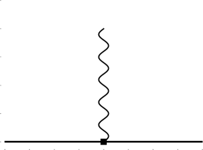
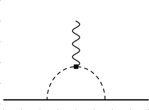
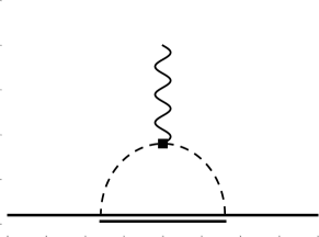
(a)         (b)        (c)

Figure 1: Feynman diagrams contributing to the magnetic moment up to $\mathcal{O}(p^{3})$ level. The single (double) solid lines refer to the spin-$\frac{1}{2}$ (spin-$\frac{3}{2}$) baryons, and dashed and wavy lines represent the mesons and photons.

Table 1: The doubly charmed baryons magnetic moments to the tree level.

$\mu$	Tree-level expression
$\Xi_{cc}^{++}$	$\frac{e}{m_{\Xi_{cc}^{++}}}(\frac{1}{3}a_{1}+2a_{2})$
$\Xi_{cc}^{+}$	$\frac{e}{m_{\Xi_{cc}^{+}}}(-\frac{1}{6}a_{1}+2a_{2})$
$\Omega_{cc}^{+}$	$\frac{e}{m_{\Omega_{cc}^{+}}}(-\frac{1}{6}a_{1}+2a_{2})$

The tree-level expression of the magnetic moment is summarized in Table 1 and the loop correction is

$$\mu_{B}^{(2,{\rm loop})} = \sum_{\phi,i}\frac{e\zeta^{(\phi,i)}\tilde{g}_{i}^{2}}{2f^{2}_{\phi}}n_{3}^{\mathrm{III}}|_{q^{2}\to 0}$$

$$= \sum_{\phi,i}\frac{e\zeta^{(\phi,i)}\tilde{g}_{i}^{2}}{2f^{2}_{\phi}}\frac{-2I_{0}\omega-J_{0}+(-2m^{2}+2\omega^{2})L_{0}}{8},$$

where the $\zeta^{(\phi,i)}$ is listed in Table 2. The loop integrals like $n^{\mathrm{III}}_{3}$ are defined in Appendix B. When substituting the forms of loop integrals using dimensional regularization into Eq. (II.1), one can obtain the same results as in Ref. Li:2017cfz .

Table 2: The coefficients of the loop correction in Eq. (II.1).

	$\zeta^{(\pi,A)}$	$\zeta^{(K,A)}$	$\zeta^{(\pi,C)}$	$\zeta^{(K,C)}$
$\Xi_{cc}^{++}$	1	1	$-\frac{1}{3}$	$-\frac{1}{3}$
$\Xi_{cc}^{+}$	$-1$	$0$	$\frac{1}{3}$	0
$\Omega_{cc}^{+}$	0	$-1$	0	$\frac{1}{3}$

In the discussion below, the momentum-space cutoff is employed to removes the spurious high-energy physics. The contribution of high energies is encoded in the low-energy constants of the local chiral Lagrangian. We use the simple covariant dipole form factor to regulate the contribution integrals Donoghue:1998bs ; Cloet:2003jm

$$\left(\frac{-\Lambda^{2}}{l^{2}-\Lambda^{2}+i\epsilon}\right)^{2}.$$ (5)

For example, $J_{0}(0)$ is regularized as

$$i\int\frac{d^{4}l}{(2\pi)^{4}}\frac{1}{(l^{2}-m^{2}+i\epsilon)(v\cdot l+i\epsilon)}$$ (6)

$$\to i\int\frac{d^{4}l}{(2\pi)^{4}}\frac{1}{(l^{2}-m^{2}+i\epsilon)(v\cdot l+i\epsilon)}\left(\frac{-\Lambda^{2}}{l^{2}-\Lambda^{2}+i\epsilon}\right)^{2}$$

$$= \frac{-1}{16\pi^{3}}\int d^{3}\vec{l}\frac{1}{\vec{l}^{2}+m^{2}}\left(\frac{\Lambda^{2}}{{\vec{l}}^{2}+\Lambda^{2}}\right)^{2}$$

$$= \frac{-\Lambda^{3}}{16\pi(\Lambda+m)^{2}}.$$

II.2 the finite-volume effect

In order to study the lattice QCD simulations, we need to consider the finite-volume effects. To introduce the finite-volume effects, the allowed three-dimensional momentum in the loop integrals is discretized

$$\vec{l}_{\vec{n}}=\frac{2\pi}{L}\vec{n},~~~~\vec{n}=(n_{x},n_{y},n_{z}),$$ (7)

where $n_{x},~n_{y}$ and $n_{z}$ take natural numbers.

If the spatial lattice extent $L$ is large enough, we can use approximate spherical symmetry and consider only the degenerate states Li:2019qvh . Then the degeneracy of there states can be calculate by $C_{3}(n)$, where $n=n^{2}_{x}+n^{2}_{y}+n^{2}_{z}$. Now using these definitions above, we rewrite the continuous integral in momentum space by

$$\int d^{3}\vec{l}\rightarrow~\left(\frac{2\pi}{L}\right)^{3}\sum_{n\in\mathbb{N}}C_{3}(n).$$ (8)

The loop integrals will be actually convergent when $n_{max}>75$.

II.3 the lattice spacing effect

We also examine the lattice spacing effect in this work. Following Refs.  Arndt:2004we ; Ren:2013wxa ; Tiburzi:2005vy , we construct the concise Wilson matrix which is proportional to the lattice spacing $a$

$$\rho_{+} = \frac{1}{2}a(u^{\dagger}c_{q}u^{\dagger}+uc_{q}u),$$ (9)

where $c_{q}$ denotes the Sheikholeslami-Wohlert coefficient matrix which reads $c_{q}={\rm diag}(c_{sw}^{u},c_{sw}^{d},c_{sw}^{s})$. The lattice QCD simulation used below gives $c_{sw}^{u/d,s}=1.715$ Can:2021ehb . The $\mathcal{O}(a)$ contributions can be canceled by incorporating the clover term into the lattice action Bar:2003mh ; Ren:2013wxa .

We can construct the Lagrangian contributing to magnetic moments with the $\rho_{+}$ operator

$$\mathcal{L}^{\mathcal{O}(a^{2})}_{int} = b_{1}m_{B}i\bar{B}[S^{\mu},S^{\nu}]\hat{F}^{+}_{\mu\nu}B{\rm Tr}(\rho_{+}\rho_{+})$$ (10)

$$+b_{2}m_{B}i\bar{B}[S^{\mu},S^{\nu}]\{\hat{F}^{+}_{\mu\nu},\rho_{+}\}B{\rm Tr}(\rho_{+})$$

$$+b_{3}m_{B}i\bar{B}[S^{\mu},S^{\nu}]\hat{F}^{+}_{\mu\nu}\rho_{+}\rho_{+}B$$

$$+b_{4}m_{B}i\bar{B}[S^{\mu},S^{\nu}]\rho_{+}\hat{F}^{+}_{\mu\nu}\rho_{+}B$$

$$+b_{5}m_{B}i\bar{B}[S^{\mu},S^{\nu}]\rho_{+}\rho_{+}\hat{F}^{+}_{\mu\nu}B.$$

The spacing effects are equal for $\mu_{\Xi_{cc}^{+}}$ and $\mu_{\Omega_{cc}^{+}}$

$$\frac{e}{6}c_{sw}^{2}a^{2}m_{B}(12b_{1}+24b_{2}+4b_{3}+4b_{4}+4b_{5})=\frac{e}{6}c_{sw}^{2}a^{2}m_{B}b,$$

where $b$ is the undetermined combined parameter.

II.4 numerical results for magnetic moments

The magnetic moments are given at large pion masses in the lattice QCD simulations as shown in Fig. 2  Can:2021ehb ; Bahtiyar:2022nqw . To relate the kaon and pion masses the following $\chi$PT relation is utilized  Liu:2018euh ; Cloet:2003jm ; Wang:2008vb

$$m_{K}^{2}=\frac{1}{2}m_{\pi}^{2}+(m^{2}_{K}-\frac{1}{2}m_{\pi}^{2})_{\rm phys}.$$ (12)

We use the lattice QCD masses in Refs. Can:2021ehb ; Bahtiyar:2022nqw for other hadrons.

Table 3: The final fitting coupling constants in three cases.

	$b$	$-\frac{1}{3}a_{1}+4a_{2}$	$\chi^{2}$
FRR	-	$1.61_{\pm 0.02}$	5.02
FRR + FV	-	$1.62_{\pm 0.02}$	4.30
FRR + FV + $\mathcal{O}(a^{2})$	$-0.07_{\pm 0.23}$	$1.83_{\pm 0.68}$	4.20

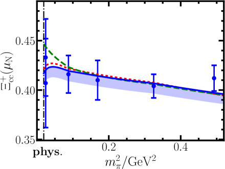
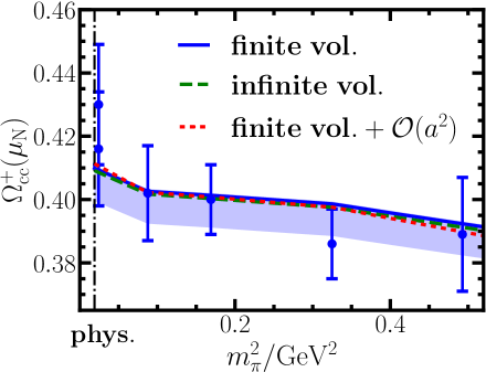
Figure 2: Magnetic moments of $\Xi_{cc}^{+}$ and $\Omega_{cc}^{+}$ as a function of $m_{\pi}$ in units of $\mu_{N}$. The lattice results are taken from Refs. Can:2021ehb ; Bahtiyar:2022nqw in 2+1 flavor QCD, shown as the blue points. The green dashed and blue solid curves label our infinite and finite results, and the red dotted curves correspond to the scenario where both discrete momenta and $\mathcal{O}(a^{2})$ are considered. The blue shaded regions illustrate the allowed probable range in our framework when we just fit the lattice results of $m_{\pi}=0.296,~0.411,~0.570$ GeV.

We study these lattice QCD data and examine the finite volume and lattice spacing effects. We choose the cutoff with 0.7 GeV. Three scenarios of fits are given in Fig. 2, and the corresponding parameters are provided in Table. 3. From the left graph in Fig. 2, one notices that the magnetic moment of $\Xi_{cc}^{+}$ near the physical pion mass seems to deviate a little from the dashed line without the finite-volume effect, which is why the $\chi^{2}$ is big in the 1st line in Table. 3. After considering the finite-volume effect, the $\chi^{2}$ decreases by about 15%. The finite-volume effect is important for interpreting the lattice QCD data.

The $\chi^{2}$ is further reduced when the lattice spacing effect is also taken into account from Table. 3, but this effect is small. The parameter for the lattice spacing effect is fitted as

$$b=-0.07\pm 0.23.$$ (13)

Its error is larger than the central value, which means the current accuracy in the lattice QCD simulations cannot effectively constrain the lattice spacing effect yet. The dotted and solid lines are also very close in Fig. 2. Therefore, in the following analysis the lattice spacing effect can be safely neglected.

For a more intuitive representation of the various loop-diagram contributions from different spin baryons, we illustrate the sizes of these contributions in Fig. 3. The loop-diagram contributions from spin-$\frac{3}{2}$ and spin-$\frac{1}{2}$ doubly charmed baryons exhibit different signs, which is because the coefficients of them have opposite signs as in Table 2. For the same reason, their magnitudes have an approximate ratio of 3:1 Liu:2012uw . The graph shows that the main finite-volume correction lies in the chiral limit Young:2004tb .

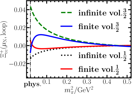
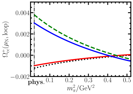
Figure 3: Comparison between the loop contributions to the magnetic moments with the intermediate baryons as the 1/2 and 3/2 doubly charmed baryons.

The dashed and solid lines exhibit an obvious deviation at small pion masses for the magnetic moment of $\Xi_{cc}^{+}$ in Figs. 2 and 3, particularly when $m_{\pi}^{2}<0.1$ GeV². If we drop the contribution from the loop momentum $\vec{l}=\vec{0}$ in the finite volume, the solid line would approach to the dashed line. The intermediate meson in Fig. 1 is pion for $\mu_{\Xi_{cc}^{+}}$ while it is kaon for $\mu_{\Omega_{cc}^{+}}$, which leads to no such phenomenon in the right graph because the heavy mass of kaon suppress the contribution in the finite volume.

The errors of lattice QCD data near the physical pion mass are relatively large, and the results at the largest pion mass may exceed the applicable range of ChPT extrapolation. Therefore, we refit the lattice data only with $m_{\pi}=0.296,~0.411,~0.570$ GeV to check whether our results are stable or not. The blue shaded regions in Fig. 2 represent this new fit with $-\frac{1}{3}a_{1}+4a_{2}=1.60_{\pm 0.02}$ and $b=0$. As we can see, the results does not change much.

The magnetic moments were studied with the dimensional regularization in Ref. Liu:2018euh , where the four $\mu_{\Xi_{cc}^{+}}$ at large pion masses on the lattice were fitted without the contributions of the excited doubly charmed baryons in Fig. 1 (c) and that gave $\chi^{2}=9.77$. We find that $\chi^{2}$ would become $98.37$ after adding Fig. 1 (c) with the dimensional regularization. However, for the same four data, the $\chi^{2}$ is only $0.72$ ($1.30$) without (with) Fig. 1 (c) if using the finite-range regularization.

In Ref. Bahtiyar:2022nqw , $\mu_{\Xi_{cc}^{++}}/\mu_{N}=0.089(45)$ is also provided at $m_{\pi}=0.156$ GeV. With the finite volume effect, we can then get $a_{1}=-1.26_{\pm 0.17}$ and $a_{2}=0.30_{\pm 0.01}$ after adding this new datum.

In an effective field theory for low-energy QCD, the magnetic moment can be systematically expanded in powers of $m^{2}_{\pi}$, which can be roughly expressed as

$$\mu_{B}=c_{0}+c_{1}m^{2}_{\pi}++I^{({\rm loop})}_{m_{\pi}}+....$$ (14)

When regulating the loop integrals using the momentum-space cutoff, the loop integrals generate the obvious cutoff dependence. Taking $J(0)$ in Eq. (6) as an example, the Taylor expansion yields

$$-\frac{\Lambda}{16\pi}+\frac{m}{8\pi}-\frac{3m^{2}}{16\pi\Lambda}+\frac{m^{3}}{4\pi\Lambda^{2}}+\mathcal{O}(m^{4}).$$ (15)

However, the $\Lambda$ variations of the loop diagrams can be absorbed by the redefinitions of the $c_{i}$ terms from the tree diagrams in principle.

We refit the above magnetic moments from the lattice QCD with different cutoffs. The variation of the coupling $-\frac{1}{3}a_{1}+4a_{2}$ is shown in Fig. 4. For sufficiently high cutoffs, the fitted coupling displays an approximately linear trend.

To investigate how the fitting quality varies with the cutoff $\Lambda$, we plot the $\chi^{2}$ values as green dots in Fig. 4. For $\Lambda<1.0$ GeV, the $\chi^{2}$ is around $5$ and the change is less than $1$, which states the physical observables are insensitive to the choice of the cutoff in this region. However, for $\Lambda>1.0$ GeV, the $\chi^{2}$ increases significantly, indicating that the convergence of perturbation expansion becomes worse. Since our analysis is limited to one-loop order, incorporating higher-order loops may reduce the cutoff dependence. The optimal fit is achieved at $\Lambda=0.7$ GeV, and thus we adopt this value for our calculations.

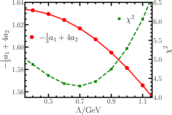
Figure 4: The red dots represent the variation trend of tree-level coupling constants with cutoff, and the green dots are the magnitude of the corresponding $\chi^{2}$ values. We connect data points with continuous lines for clarity.

II.5 magnetic form factors

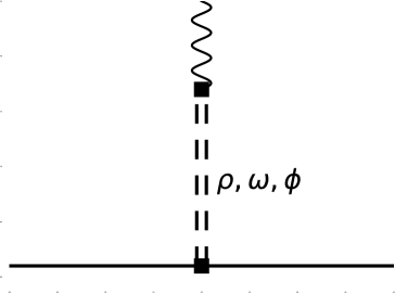
Figure 5: The vector meson dominance diagram for the magnetic form factors of the doubly charmed baryons.

To study the magnetic form factors, we need to consider the vector meson contribution as in Fig. 5 HillerBlin:2018gjw . The Lagrangians involved are listed in Appendix A. The results can be expressed as

$$G_{M}^{B}(q^{2})=g_{V}^{B}\frac{C_{VB}F_{V}}{m_{V}}\frac{q^{2}}{q^{2}-m_{V}^{2}}.$$ (16)

Due to the significant breaking of SU(3) symmetry for the vector mesons, two couplings, $g_{V}^{\Xi_{cc}}$ and $g_{V}^{\Omega_{cc}}$, are introduced. The coefficients $C_{VB}$ are listed in Table II of Ref. HillerBlin:2018gjw . The above equation shows the vector mesons do not contribute to $G_{M}$ as $q^{2}\rightarrow 0$, and that is why we do not mention them for the magnetic moments. The dependence of $G_{M}$ can also be empirically parameterized as dipole from factor $G_{M}(Q^{2})=G_{M}(0)/(1+Q^{2}/0.71~{\rm GeV^{2}})^{2}$ Kubis:2000zd ; Kubis:2000aa ; HillerBlin:2017syu ; Wang:2007iw ; Perdrisat:2006hj ; Mergell:1995bf .

In order to introduce the dependence of vector meson masses on $m_{\pi}$, we use Zhou:2014ila

$$m^{2}_{\rho}=m^{2}_{\omega} = m_{0}^{2}+2\lambda_{m}m^{2}_{\pi}+\lambda_{0}(2m_{K}^{2}+m_{\pi}^{2}),$$

$$m^{2}_{\phi} = m_{0}^{2}+4\lambda_{m}m_{K}^{2}-2\lambda_{m}m_{\pi}^{2}+\lambda_{0}(2m_{K}^{2}+m_{\pi}^{2}),$$ (17)

where $m_{0}\approx 0.712$ GeV, $\lambda_{m}\approx 0.489$ and $\lambda_{0}\approx 0.126$. There are also different pion mass dependence for them Danilkin:2011fz ; Ren:2024frr , but this discrepancy does not impact our ultimate conclusion.

We obtain the tree-level couplings by fitting the lattice QCD results from Tsukuba actions, where the pion mass is $156$ MeV Bahtiyar:2022nqw , as shown by the red points in Fig. 6. Both the contributions from vector mesons and discrete-momentum effects are considered. The final results are $g_{V}^{\Xi_{cc}}=8.96_{\pm 0.99}$ and $g_{V}^{\Omega_{cc}}=28.58_{\pm 2.65}$.

These parameters are used to calculate the trend as $Q^{2}$ increases for the others pion masses in Fig. 6. The different pion masses exhibit almost identical dependence on $Q^{2}$ for $\Omega_{cc}^{+}$, as the masses of $c$ and $s$ quarks do not change obviously in the lattice configurations for different pion masses. For $\Xi_{cc}^{+}$, the left graph clearly shows that the slope decreases with the increasing pion mass.

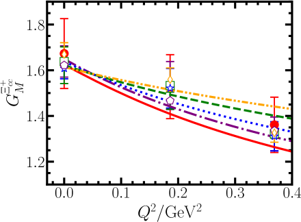
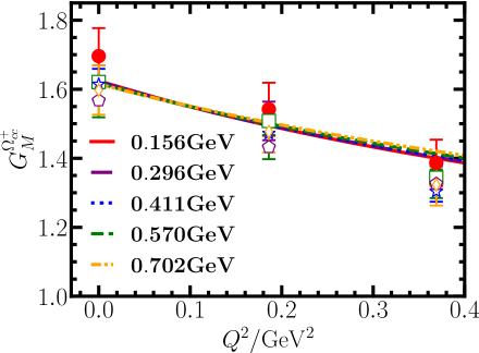
Figure 6: Comparison between the magnetic form factors from the lattice QCD data and our results. The lattice QCD data are taken from Refs. Bahtiyar:2022nqw ; Can:2021ehb . The contribution of spin-$\frac{3}{2}$ baryons and vector meson dominance model in the finite volume are considered.

After obtaining the $g_{V}^{B}$ and tree-level couplings in Table 3, we can calculate the mean square radius $\left<r^{2}_{M}\right>$ in the infinite volume at the physical pion mass. The values is 0.30 fm² for $\Xi_{cc}^{+}$ and 0.15 fm² for $\Omega_{cc}^{+}$. They are about 1/3 of the $\left<r^{2}_{M}\right>_{\rm nucleon}$, similar to those extended on-mass-shell scheme in Ref. HillerBlin:2018gjw .

III the transition magnetic form factors

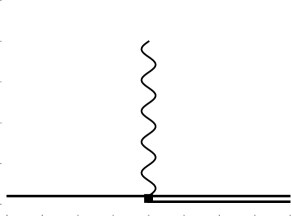
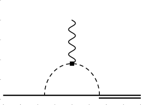
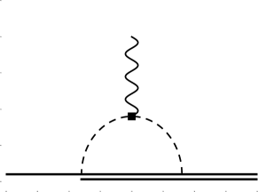
(a)         (b)        (c)

Figure 7: Feynman diagrams for the transition magnetic moments.

The matrix elements of electromagnetic current between spin-$\frac{1}{2}$ and spin-$\frac{3}{2}$ baryon are defined as. Jones:1972ky ; Bahtiyar:2022nqw

$$\langle\Psi^{*\rho}(p^{\prime})|J_{\mu}|\Psi(p)\rangle=\sqrt{\frac{2}{3}}e\bar{u}^{\rho}(p^{\prime})\mathcal{O}_{\rho\mu}(p^{\prime},p)u(p).$$ (18)

In the framework of HBChPT, the tensor $\mathcal{O}_{\rho\mu}$ can be parametrized in three Lorentz invariant terms

$$\mathcal{O}_{\rho\mu}(p^{\prime},p) = 2G_{1}(q_{\rho}S_{\mu}-q\cdot Sg_{\rho\mu})$$ (19)

$$+G_{2}\frac{2m_{T}}{m_{B}+m_{T}}(q_{\rho}v_{\mu}-q\cdot vg_{\rho\mu})q\cdot S$$

$$+G_{3}\frac{2}{m_{B}+m_{T}}(q_{\mu}q_{\rho}-q^{2}g_{\rho\mu})q\cdot S.$$

Here $u^{\rho}(p)$ is a spin-vector in the Rarita-Schwinger formalism satisfying $v_{\rho}u^{\rho}(p)=0$ and $\gamma_{\rho}u^{\rho}(p)=0$ Nozawa:1990gt ; Hemmert:1997wz ; Hemmert:1996xg ; Jenkins:1991es ; Rarita:1941mf . The transition magnetic form factor $G_{M1}(q^{2})$ is expressed as

$$G_{M1}(q^{2}) = \frac{m_{B}}{3(m_{T}+m_{B})}[G_{1}\frac{(m_{T}+m_{B})(3m_{T}+m_{B})-q^{2}}{m_{T}}$$ (20)

$$+G_{2}(m_{T}^{2}-m_{B}^{2})+2q^{2}G_{3}].$$

III.1 expressions in the physical world

There are three Feynman diagrams that contribute to $G_{M1}$ up to $\mathcal{O}(p^{3})$, which are depicted in Fig. 7. The tree-level diagram comes from Lagrangian in Eq. (A), while the baryon-meson vertex of the loop diagrams comes from the interaction Lagrangian in Eq. (A). The tree diagram only contribtutes to $G_{1}$ and can be expressed as

$$G_{M1}^{(2,{\rm tree})}=\gamma_{B}\frac{(m_{T}+m_{B})(3m_{T}+m_{B})-q^{2}}{4m_{T}m_{B}}.$$ (21)

The loop contributions are

$$G_{M1}^{(3,{\rm loop})}=G_{M1}^{(3,b)}+G_{M1}^{(3,c)},$$ (22)

where

$$G_{M1}^{(3,b)}=$$

$$\frac{(m_{T}+m_{B})(3m_{T}+m_{B})-q^{2}}{8m_{T}}\sum_{i=\pi,K}\left(\alpha_{AC}^{(i)}\frac{\tilde{g}_{A}\tilde{g}_{C}}{4f^{2}_{i}}\right)\left(n_{3}^{\mathrm{III}}+n_{1}^{\mathrm{II}}\right)$$

$$+\frac{(m^{2}_{T}-m^{2}_{B})(m_{B}+m_{T})}{8m_{T}}\sum_{i=\pi,K}\left(\beta_{AC}^{(i)}\frac{\tilde{g}_{A}\tilde{g}_{C}}{4f^{2}_{i}}\right)\left(n_{2}^{\mathrm{III}}+n_{4}^{\mathrm{II}}\right)$$

$$+\frac{(m_{B}+m_{T})q^{2}}{4}\sum_{i=\pi,K}\left(\zeta_{AC}^{(i)}\frac{\tilde{g}_{A}\tilde{g}_{C}}{4f^{2}_{i}}\right)\left(2n_{1}^{\mathrm{III}}+3n_{2}^{\mathrm{II}}+n_{1}^{\mathrm{I}}\right),$$ (23)

and

$$G_{M1}^{(3,c)}=$$

$$\frac{(m_{T}+m_{B})(3m_{T}+m_{B})-q^{2}}{8m_{T}}\sum_{i=\pi,K}\left(\alpha_{BC}^{(i)}\frac{\tilde{g}_{B}\tilde{g}_{C}}{4f^{2}_{i}}\right)\left(n_{3}^{\mathrm{III}}-2n_{1}^{\mathrm{II}}\right)$$

$$+\frac{(m^{2}_{T}-m^{2}_{B})(m_{B}+m_{T})}{8m_{T}}\sum_{i=\pi,K}\left(\beta_{BC}^{(i)}\frac{\tilde{g}_{B}\tilde{g}_{C}}{4f^{2}_{i}}\right)\left(n_{2}^{\mathrm{III}}+n_{4}^{\mathrm{II}}\right)$$

$$+\frac{(m_{B}+m_{T})q^{2}}{4}\sum_{i=\pi,K}\left(\zeta_{BC}^{(i)}\frac{\tilde{g}_{B}\tilde{g}_{C}}{4f^{2}_{i}}\right)\left(2n_{1}^{\mathrm{III}}+3n_{2}^{\mathrm{II}}+n_{1}^{\mathrm{I}}\right).$$ (24)

We summarize the coefficients $\gamma_{B}$, $\alpha_{AC}^{(i)}$ $\alpha_{BC}^{(i)}$, $\beta_{AC}^{(i)}$, $\beta_{BC}^{(i)}$, $\zeta_{AC}^{(i)}$ and $\zeta_{BC}^{(i)}$ in Table 4. The forms of $n^{\mathrm{I}}_{1}$, $n^{\mathrm{II}}_{1}$, $n^{\mathrm{II}}_{2}$, $n^{\mathrm{II}}_{4}$, $n^{\mathrm{III}}_{1}$, $n^{\mathrm{III}}_{2}$ and $n^{\mathrm{III}}_{3}$ are also obtained by solving the Lorentzian invariant structures in the appendix, which have been evaluated in the rest-frame of spin-$\frac{3}{2}$ baryon Gellas:1998wx ; Arndt:2003vd .

Table 4: The coefficients of the tree and loop correction to $G_{M1}$ from Eq. (21) and Eq. (III.1).

B	$\gamma_{B}$
$\Xi_{cc}^{++}$	$-\frac{1}{3}a_{3}-2a_{4}$
$\Xi_{cc}^{+}$	$\frac{1}{6}a_{3}-2a_{4}$
$\Omega_{cc}^{+}$	$\frac{1}{6}a_{3}-2a_{4}$

B	$\alpha_{BC}^{(\pi)}$	$\alpha_{AC}^{(\pi)}$	$\alpha_{BC}^{(K)}$	$\alpha_{AC}^{(K)}$	$\beta_{BC}^{(\pi)}$	$\beta_{AC}^{(\pi)}$	$\beta_{BC}^{(K)}$	$\beta_{AC}^{(K)}$	$\zeta^{(\pi)}_{BC}$	$\zeta^{(\pi)}_{AC}$	$\zeta^{(K)}_{BC}$	$\zeta^{(K)}_{AC}$
$\Xi_{cc}^{++}$	$-\frac{2}{3}$	$2$	$-\frac{2}{3}$	$2$	$-\frac{2}{3}$	$2$	$-\frac{2}{3}$	$2$	$-\frac{1}{3}$	$1$	$-\frac{1}{3}$	$1$
$\Xi_{cc}^{+}$	$\frac{2}{3}$	$-2$	0	0	$\frac{2}{3}$	$-2$	0	0	$\frac{1}{3}$	$-1$	0	0
$\Omega_{cc}^{+}$	0	0	$\frac{2}{3}$	$-2$	0	0	$\frac{2}{3}$	$-2$	0	0	$\frac{1}{3}$	$-1$

The method of deriving loop integrals is universally applicable, and it has been described in detail in the appendix of Ref. Meng:2019ilv . The results conform the following relationship,

$$2(n_{1}^{\rm II}+n_{3}^{\rm III})+2(n_{2}^{\rm III}+n_{4}^{\rm II})q\cdot v+(2n_{1}^{\rm III}+3n_{2}^{\rm II}+n_{1}^{\rm I})q^{2}=-2n_{3}^{\rm III},$$

and this ensures that the numerical matrix elements of electromagnetic current still has the tensor $\mathcal{O}_{\rho\mu}$ structure which can be obtained with the symmetry analysis.

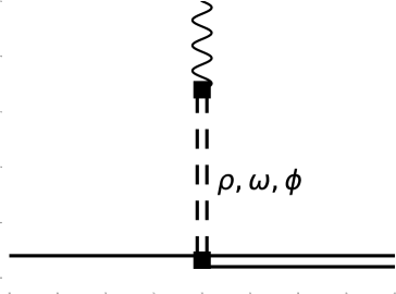
Figure 8: The vector meson dominance diagram for the transition magnetic form factors.

Similarly, we consider the vector meson contribution as in Fig. 8  HillerBlin:2018gjw ; Aliev:2021hqq ; Aliyev:2022rrf . The specific Lagrangians of the interaction are provided in Eq. (54) and Eq. (61) in the appendix. It only contributes through $G_{1}$ as

$$G_{M1}^{({\rm vec.})}=\xi_{V}\frac{\sqrt{3}d^{\Xi_{cc}/\Omega_{cc}}_{V}F_{V}}{4m_{V}m_{B}}\frac{q^{2}}{q^{2}-m^{2}_{V}}\frac{(m_{T}+m_{B})(3m_{T}+m_{B})-q^{2}}{4m_{T}},$$ (26)

where the $\xi_{V}$ values are listed in Table 5.

Table 5: The coefficients $\xi_{V}$ of vector meson contribution in Eq. (III.1).

	$\Xi_{cc}^{++}$	$\Xi_{cc}^{+}$	$\Omega_{cc}^{+}$
$\rho$	$\frac{\sqrt{2}}{2}$	$-\frac{\sqrt{2}}{2}$	0
$\omega$	$\frac{\sqrt{2}}{6}$	$\frac{\sqrt{2}}{6}$	0
$\phi$	0	0	$-\frac{\sqrt{2}}{3}$

III.2 numerical results

The lattice QCD simulations provided the multipole form factors of doubly charmed baryons at $m_{\pi}=0.156$ GeV and the transfer momentum square $Q^{2}=-q^{2}\approx 0.18$ GeV² with the spatial lattice extent $L=2.9$ fm in Refs. Bahtiyar:2018vub ; Bahtiyar:2019ykq , and we present them in Fig. 9. We explicitly consider the mass splitting, $\delta\approx 68$ MeV, between spin-$\frac{1}{2}$ and spin-$\frac{3}{2}$ doubly charmed baryons from the lattice QCD results.

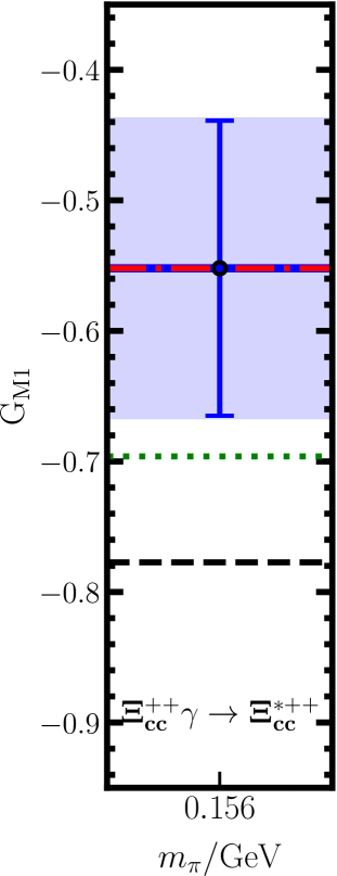
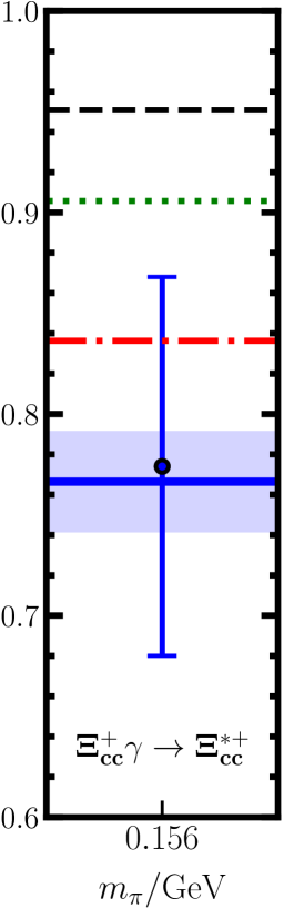
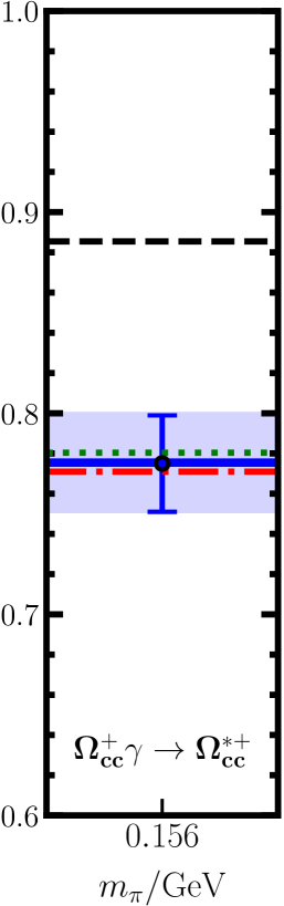
Figure 9: The magnetic multipole transition form factors $G_{M1}$ of doubly charmed baryons at $m_{\pi}=0.156$ GeV and $Q^{2}=-q^{2}\approx 0.18$ GeV² with the spatial lattice extent $L=2.9$ fm. With the corrections of vector mesons, the solid blue lines represent the results in the finite volume while the green dotted lines label our infinite-volume results. The black dashed lines label our finite-volume results for $d_{V}=0$, that is, the vector meson contributions are turned off. The red dash-dotted lines represent the new fits by adjusting $a_{i}$ with $d_{V}=0$. The blue shaded regions illustrate the allowed ranges based on the fit within our framework. The lattice QCD data are taken from Ref. Bahtiyar:2018vub

For the vector meson contributions, we utilize the heavy quark symmetry to relate the $TBV$ and $BBV$ couplings as mentioned in the appendix, and thus $d_{V}^{\Xi_{cc}}=g_{V}^{\Xi_{cc}}=8.96_{\pm 0.99}$ and $d_{V}^{\Omega_{cc}}=g_{V}^{\Omega_{cc}}=28.58_{\pm 2.65}$. Our numerical results are presented in Fig. 9 with $\Lambda=0.7$ GeV. The blue lines represent the fit that includes the contributions of vector mesons for the finite-volume version, and the fitted parameters are listed in Table 6. We also plot the allowed regions of this fit as the blue shades. It clearly shows that the HBChPT with FRR can describe the lattice QCD results well.

We fix $a_{3}$ and $a_{4}$ as in Table 6, replace the sum of the discrete momenta with the integral of the continue momenta for the loop diagrams, and obtain the green dotted lines corresponding to the results in the infinite volume. The large difference between the blue solid lines and the green dotted lines indicates the finite-volume effect is obvious at the current stage.

To show the effect of the vector mesons, we turn off them by setting $d_{V}=0$ and obtain the black dashed lines with $a_{i}$ in Table 6. They deviate about $2\sigma$ from the lattice QCD center data, which states that the vector mesons are important for the transition form factors even at small $Q^{2}=-q^{2}\approx 0.18$ GeV². Even if we refit the lattice QCD data by adjusting $a_{i}$ without the vector mesons, the best fit as shown by the red dash-dotted lines exhibits a little tention with the lattice QCD datum in the middle graph of Fig. 9.

Table 6: The fitted couplings.

$a_{3}$	$a_{4}$
$1.89_{\pm 0.15}$	$-0.11_{\pm 0.01}$

We separate the $G_{M1}$ into four parts: the tree-level term and the loop terms proportional to $G_{1}$, $G_{2}$, and $G_{3}$. The tree diagram only itself will lead to zero for $G_{2}$ and $G_{3}$. Taking the $\Omega_{cc}$ case at $q^{2}=-0.18$ GeV² and $m_{\pi}=156$ MeV as an example,

$$G^{\Omega^{+}_{cc}}_{M1}=0.756+[0.019+0.001-0.002]=0.774.$$ (27)

It is clear that the tree diagram dominates in our framework, and the loops give about 15% corrections.

The $G_{3}$ related term above is tiny and will be strictly 0 at $q^{2}=0$:

$$G^{\Omega^{+}_{cc}}_{M1}(q^{2}=0)=0.865+[0.065-0.062+0]=0.868.$$ (28)

The third lines in Eq. (III.1) and Eq. (III.1) correspond to the $G_{3}$ term and cancel themselves out as $q^{2}\rightarrow 0$ due to the constraints from heavy quark symmetry on the couplings $\tilde{g}_{A}$, $\tilde{g}_{B}$, and $\tilde{g}_{C}$ which appear in the loop diagrams. However, with a slight breaking of heavy quark symmetry, for example, $\tilde{g}_{A}\to\tilde{g}_{A}$, $\tilde{g}_{B}\to 0.95\tilde{g}_{B}$, and $\tilde{g}_{C}\to\tilde{g}_{C}$, one has

$$q^{2}G_{3}(q^{2})\,\big{|}_{q^{2}\to 0}\neq 0,$$ (29)

and

$$G^{\Omega^{+}_{cc}}_{M1}(q^{2}=0)=0.865+[0.061-0.015-0.043]=0.868.$$ (30)

If the static $G_{3}$ terms can be extracted accurately on the lattice, the breaking of the heavy quark symmetry would be understood better.

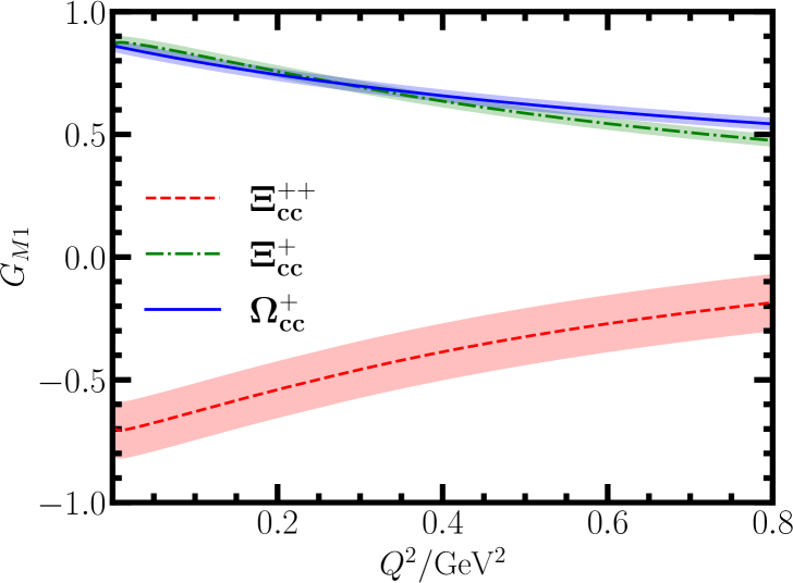
Figure 10: Our predictions for the transition magnetic form factors $G_{M1}$ as the $Q^{2}$ increases with $m_{\pi}=0.156$ GeV and $L=2.9$ fm.

Finally, we predict the trend of $G_{M1}$ in Fig. 10 at $m_{\pi}=0.156$ GeV and $L=2.9$ fm for the range $Q^{2}=0\sim 0.8$ GeV² with the fitting couplings in Table 6. From the figure, the $G_{M1}^{\Xi_{cc}^{++}}$ exhibits the opposite trend compared to the others. The main reason is that the contributions from the vector mesons have different signs for these transition form factors, which can be easily estimated from Table 5. We hope they can be examined in future.

IV summary

In this work, we employ HBChPT to study the magnetic form factors and transition magnetic form factors of the doubly charmed baryons up to $\mathcal{O}(p^{3})$. The loop integrals are dealt with the finite-range regularization. We found that finite volume effects are important for interpreting the lattice QCD data, while the lattice spacing effect is not obvious compared to the current accuracy of simulation. We can simultaneously explain three different groups of the lattice QCD data very well as shown in Figs. 2, 6 and 9.

We consider both spin-$\frac{1}{2}$ and spin-$\frac{3}{2}$ doubly charmed baryons as the intermediate states in the loop diagrams. For the magnetic moments, the spin-$\frac{3}{2}$ loop contributions are relatively bigger and have different signs from the spin-$\frac{1}{2}$ ones.

The finite-volume effects improve the consistency of our results with lattice QCD data, particularly in the small pion-mass region. This improvement arises from the contribution of the zero-momentum mode ($\vec{l}=\vec{0}$) in finite volumes. In contrast, the finite-volume corrections for the $\Omega^{+}_{cc}$ baryon are less pronounced, as the loops involve kaons which are less sensitive to these effects. For the magnetic form factors, the contributions from vector mesons are introduced to examine the $q^{2}$ dependence of $G_{M}$. These corrections become increasingly important as $q^{2}$ grows.

We have also studied the transition form factors $G_{M1}$ for the process $\Xi_{cc}^{++}\gamma\rightarrow\Xi_{cc}^{*++}$, $\Xi_{cc}^{+}\gamma\rightarrow\Xi_{cc}^{*+}$ and $\Omega_{cc}^{+}\gamma\rightarrow\Omega_{cc}^{*+}$. The finite-volume effects are also significant for the transition magnetic form factors when fitting to the lattice QCD results. The vector mesons play a crucial role in the transition form factors, even at small momentum transfer, $Q^{2}=-q^{2}\approx 0.18$ GeV². We carefully examine the loop contributions associated with the $G_{1}$, $G_{2}$, and $G_{3}$ terms, and the $G_{3}$ terms becomes bigger if the heavy quark symmetry is not strictly kept. Furthermore, we provide predictions for the transition form factors as a function of $Q^{2}$.

We have systematically studied the electromagnetic properties of the doubly charmed baryons within HBChPT, which can also help us understand the nonperturbative strong interactions. We expect our study can be further confirmed in the future lattice QCD calculations or experiments.

Appendix A effective Lagrangians

We construct the chiral Lagrangians following Refs. Scherer:2002tk ; Li:2017pxa ; Li:2017cfz . The spin-$\frac{1}{2}$ doubly charmed baryon fields are collected in

$$\Psi=\left(\begin{array}[]{c}\Xi^{++}_{cc}\\ \Xi^{+}_{cc}\\ \Omega^{+}_{cc}\end{array}\right)~~~\Rightarrow~~~\left(\begin{array}[]{c}ccu\\ ccd\\ ccs\\ \end{array}\right),$$ (37)

the spin-$\frac{3}{2}$ doubly charmed baryon fields are denoted by the Rarita-Schwinger fields as Rarita:1941mf

$$\Psi^{*\rho}=\left(\begin{array}[]{c}\Xi^{*++}_{cc}\\ \Xi^{*+}_{cc}\\ \Omega^{*+}_{cc}\end{array}\right)^{\rho}~~\Rightarrow~~\left(\begin{array}[]{c}ccu\\ ccd\\ ccs\\ \end{array}\right)^{\rho},$$ (44)

and the pseudoscalar meson fields are introduced as

$$\phi=\left(\begin{array}[]{ccc}\pi^{0}+\frac{1}{\sqrt{3}}\eta&\sqrt{2}\pi^{+}&\sqrt{2}K^{+}\\ \sqrt{2}\pi^{-}&-\pi^{0}+\frac{1}{\sqrt{3}}\eta&\sqrt{2}K^{0}\\ \sqrt{2}K^{-}&\sqrt{2}\bar{K}^{0}&-\frac{2}{\sqrt{3}}\eta\end{array}\right).$$ (48)

We choose the nonlinear realization of the chiral symmetry,

$$U=u^{2}=\exp(i\phi/f_{\phi}),$$ (49)

and $f_{\phi}$ denote the decay constant of pseudoscalar meson, and $f_{\pi}=92.4$ MeV and $f_{K}=113$ MeV are used in this work. The chiral axial vector field are defined as Scherer:2002tk ,

$$u_{\mu} = \frac{1}{2}i[u^{\dagger}(\partial_{\mu}-ir_{\mu})u-u(\partial-il_{\mu})u^{\dagger}],$$ (50)

where $r_{\mu}=l_{\mu}=-eQA_{\mu}$, and $Q=$ diag $(2/3,-1/3,-1/3)$ for the pure meson Lagrangians while $Q=$ diag $(2,1,1)$ for baryon fields.

The $\mathcal{O}(p^{2})$ Lagrangian contributing to the magnetic moments of doubly charmed baryons at the tree level reads

$$\mathcal{L}^{(2)}_{\gamma BB}=a_{1}\frac{-i}{4m_{B}}\bar{B}[S^{\mu},S^{\nu}]\hat{F}^{+}_{\mu\nu}B+a_{2}\frac{-i}{4m_{B}}\hat{B}[S^{\mu},S^{\nu}]B{\rm Tr}(F^{+}_{\mu\nu}),$$

where $a_{1,2}$ are the low-energy constants, and the traceless operator $\hat{F}^{+}_{\mu\nu}=F^{+}_{\mu\nu}-\frac{1}{3}{\rm Tr}(F^{+}_{\mu\nu})$. The chirally covariant QED field strength tensor $F^{+}_{\mu\nu}=u^{\dagger}F^{R}_{\mu\nu}u+uF^{L}_{\mu\nu}u^{\dagger}$, where $F^{R}_{\mu\nu}=\partial_{\mu}r_{\nu}-\partial_{\nu}r_{\mu}-i[r_{\mu},r_{\nu}]$ and $F^{L}_{\mu\nu}=\partial_{\mu}l_{\nu}-\partial_{\nu}l_{\mu}-i[l_{\mu},l_{\nu}]$.

The $\mathcal{O}(p^{2})$ tree-level terms which contribute the spin-$\frac{1}{2}$ to spin-$\frac{3}{2}$ transition magnetic moment are

$$\mathcal{L}_{int}^{(2)}=a_{3}\frac{-i}{2m_{B}}\bar{T}^{\mu}\hat{F}^{+}_{\mu\nu}S^{\nu}B+a_{4}\frac{-i}{2m_{B}}\bar{T}^{\mu}S^{\nu}B\mathrm{Tr}(F^{+}_{\mu\nu})+\mathrm{H.c.}$$

The $\mathcal{O}(p^{2})$ pure meson Lagrangian is

$$\mathcal{L}^{(2)}_{\gamma MM}=\frac{f^{2}_{0}}{4}{\rm Tr}[\nabla_{\mu}U(\nabla^{\mu}U)^{\dagger}],$$ (53)

with $\nabla_{\mu}U=\partial_{\mu}U-ir_{\mu}U+iUl_{\mu}.$

The Lagrangian which describes the interaction of vector mesons and photons is given by HillerBlin:2018gjw ; Borasoy:1995ds

$$\mathcal{L}_{\gamma}=-\frac{1}{2\sqrt{2}}\frac{F_{V}}{m_{V}}\mathrm{Tr}[V_{\mu\nu}F^{+\mu\nu}]$$ (54)

where $F_{V}$ is the decay constants of $V\rightarrow e^{+}e^{-}$ and $V_{\mu\nu}=\partial_{\mu}V_{\nu}-\partial_{\nu}V_{\mu}$ with

$$V_{\mu}=\left(\begin{array}[]{ccc}\frac{1}{\sqrt{2}}\rho^{0}+\frac{1}{\sqrt{2}}\omega&\rho^{+}&K^{*+}\\ \rho^{-}&-\frac{1}{\sqrt{2}}\rho^{0}+\frac{1}{\sqrt{2}}\omega&K^{*0}\\ K^{*-}&\bar{K}^{*0}&\phi\end{array}\right)_{\mu}.$$ (58)

In the HBChPT scheme, the $\mathcal{O}(p^{1})$ Lagrangian describing the interaction between two baryons and a pseudoscalar meson read

$$\mathcal{L}^{(1)}_{int}=\tilde{g}_{A}\bar{B}S^{\mu}u_{\mu}B+\tilde{g}_{B}\bar{T}^{\rho}S^{\mu}u_{\mu}T_{\rho}+\frac{\tilde{g}_{C}}{2}[\bar{T}^{\mu}u_{\mu}B+\bar{B}u_{\mu}T^{\mu}].$$

To investigate the impact of vector mesons on the magnetic form factors and transition form factors, we refer to Ref. HillerBlin:2018gjw for the following Lagrangians within the HBChPT framework,

$$\mathcal{L}_{VBB}=-\frac{ig_{V}}{2m_{B}}\bar{B}[S^{\mu},S^{\nu}]V_{\nu\mu}B,$$ (60)

$$\mathcal{L}_{VBT}=-\frac{i\sqrt{3}d_{V}}{2m_{B}}\bar{T}^{\mu}V_{\mu\nu}S^{\nu}B.$$ (61)

Utilizing the heavy quark symmetry, the spin-$\frac{1}{2}$ and spin-$\frac{3}{2}$ states can be unified in a superfield Falk:1991nq ; Meng:2018zbl

$$\psi^{\mu}=T^{\mu}-\sqrt{\frac{1}{3}}(\gamma^{\mu}+v^{\mu})\gamma_{5}B.$$ (62)

With the Lagrangian $\kappa\bar{\psi}^{\mu}\not{u}\gamma_{5}\psi_{\mu}$ describing the interaction between two baryons and a pseudoscalar meson Wang:2018cre , one can obtain the relations for the pseudoscalar couplings in Eq. (A):

$$\tilde{g}_{B}=3\tilde{g}_{A},\quad\tilde{g}_{C}=2\sqrt{3}\tilde{g}_{A}.$$ (63)

Similarly, the vector couplings satisfy the following relation from the Lagrangian $\displaystyle\frac{i\kappa_{V}}{m_{B}}\bar{\psi}^{\mu}V_{\mu\nu}\psi^{\nu}$:

$$d_{V}=g_{V}.$$ (64)

Appendix B loop integrals

We collect some common loop functions as follows Wang:2018atz ; Scherer:2002tk ; Meng:2019ilv

$$\Delta = i\int\frac{d^{4}l}{(2\pi)^{4}}\frac{1}{l^{2}-m^{2}+i\epsilon},$$ (65)

$$I_{0}(q^{2}) = i\int\frac{d^{4}l}{(2\pi)^{4}}\frac{1}{(l^{2}-m^{2}+i\epsilon)[(l+q)^{2}-m^{2}+i\epsilon]},$$

$$J_{0}(\omega) = i\int\frac{d^{4}l}{(2\pi)^{4}}\frac{1}{(l^{2}-m^{2}+i\epsilon)(v\cdot l+\omega+i\epsilon)},$$ (67)

$$i\int\frac{d^{4}l}{(2\pi)^{4}}\frac{[1,l_{\alpha},l_{\alpha}l_{\beta},l_{\nu}l_{\alpha}l_{\beta}]}{(l^{2}-m^{2}+i\epsilon)[(l+q)^{2}-m^{2}+i\epsilon](v\cdot l+\omega+i\epsilon)}$$

$$=[L_{0}(\omega),L_{\alpha},L_{\alpha\beta},L_{\nu\alpha\beta}],~~~~~~~~~~~~~~~~~~~~~~~~~~~~~~~~~~~~~~~~~~~$$

(68)

where

$$L_{\alpha} = n^{\rm I}_{1}q_{\alpha}+n^{\rm I}_{2}v_{\alpha},$$

$$L_{\alpha\beta} = n^{\rm II}_{1}g_{\alpha\beta}+n^{\rm II}_{2}q_{\alpha}q_{\beta}+n^{\rm II}_{3}v_{\alpha}v_{\beta}+n^{\rm II}_{4}(v_{\alpha}q_{\beta}+q_{\alpha}v_{\beta}),$$

$$L_{\nu\alpha\beta} = n^{\rm III}_{1}q_{\nu}q_{\alpha}q_{\beta}+n^{\rm III}_{2}(q_{\nu}q_{\alpha}v_{\beta}+q_{\nu}q_{\beta}v_{\alpha}+q_{\alpha}q_{\beta}v_{\nu})$$

$$+n^{\rm III}_{3}(q_{\nu}g_{\alpha\beta}+q_{\beta}g_{\nu\alpha}+q_{\alpha}g_{\nu\beta})$$

$$+n^{\rm III}_{4}(q_{\nu}v_{\alpha}v_{\beta}+q_{\alpha}v_{\nu}v_{\beta}+q_{\beta}v_{\nu}v_{\alpha})$$

$$+n^{\rm III}_{5}(g_{\nu\beta}v_{\alpha}+g_{\nu\alpha}v_{\beta}+g_{\alpha\beta}v_{\nu})+n^{\rm III}_{6}v_{\nu}v_{\alpha}v_{\beta}.$$

References

- (1) A. Ocherashvili et al. [SELEX], Confirmation of the double charm baryon Xi+(cc)(3520) via its decay to p D+ K-, Phys. Lett. B 628, 18-24 (2005) [arXiv:hep-ex/0406033 [hep-ex]].
- (2) R. Aaij et al. [LHCb], Precision measurement of the mass, JHEP 02, 049 (2020) [arXiv:1911.08594 [hep-ex]].
- (3) R. Aaij et al. [LHCb], First Observation of the Doubly Charmed Baryon Decay , Phys. Rev. Lett. 121, no.16, 162002 (2018) [arXiv:1807.01919 [hep-ex]].
- (4) S. P. Ratti, New results on c-baryons and a search for cc-baryons in FOCUS, Nucl. Phys. B Proc. Suppl. 115, 33-36 (2003)
- (5) B. Aubert et al. [BaBar], Search for doubly charmed baryons Xi(cc)+ and Xi(cc)++ in BABAR, Phys. Rev. D 74, 011103 (2006) [arXiv:hep-ex/0605075 [hep-ex]].
- (6) R. Aaij et al. [LHCb], Search for the doubly charmed baryon in the final state, JHEP 12, 107 (2021) [arXiv:2109.07292 [hep-ex]].
- (7) R. Chistov et al. [Belle], Observation of new states decaying into Lambda(c)+ K- pi+ and Lambda(c)+ K0(S) pi-, Phys. Rev. Lett. 97, 162001 (2006) [arXiv:hep-ex/0606051 [hep-ex]].
- (8) R. Aaij et al. [LHCb], Measurement of the Lifetime of the Doubly Charmed Baryon , Phys. Rev. Lett. 121, no.5, 052002 (2018) [arXiv:1806.02744 [hep-ex]].
- (9) R. Aaij et al. [LHCb], Measurement of production in collisions at TeV, Chin. Phys. C 44, no.2, 022001 (2020) [arXiv:1910.11316 [hep-ex]].
- (10) R. Aaij et al. [LHCb], Observation of the doubly charmed baryon decay , JHEP 05, 038 (2022) [arXiv:2202.05648 [hep-ex]].
- (11) R. Aaij et al. [LHCb], A search for decays, JHEP 10, 124 (2019) [arXiv:1905.02421 [hep-ex]].
- (12) R. Aaij et al. [LHCb], Search for the doubly charmed baryon , Sci. China Phys. Mech. Astron. 64, no.10, 101062 (2021) [arXiv:2105.06841 [hep-ex]].
- (13) M. Mattson et al. [SELEX], First Observation of the Doubly Charmed Baryon , Phys. Rev. Lett. 89, 112001 (2002) [arXiv:hep-ex/0208014 [hep-ex]].
- (14) R. Aaij et al. [LHCb], Observation of the doubly charmed baryon , Phys. Rev. Lett. 119, no.11, 112001 (2017) [arXiv:1707.01621 [hep-ex]].
- (15) D. B. Lichtenberg, Magnetic Moments of Charmed Baryons in the Quark Model, Phys. Rev. D 15, 345 (1977)
- (16) B. Julia-Diaz and D. O. Riska, Baryon magnetic moments in relativistic quark models, Nucl. Phys. A 739, 69-88 (2004) [arXiv:hep-ph/0401096 [hep-ph]].
- (17) A. Faessler, T. Gutsche, M. A. Ivanov, J. G. Korner, V. E. Lyubovitskij, D. Nicmorus and K. Pumsa-ard, Magnetic moments of heavy baryons in the relativistic three-quark model, Phys. Rev. D 73, 094013 (2006) [arXiv:hep-ph/0602193 [hep-ph]].
- (18) S. N. Jena and D. P. Rath, Magnetic Moments of Light, Charmed and Flavored Baryons in a Relativistic Logarithmic Potential, Phys. Rev. D 34, 196-200 (1986)
- (19) B. Patel, A. K. Rai and P. C. Vinodkumar, Masses and Magnetic Moments of Charmed Baryons Using Hyper Central Model, [arXiv:0803.0221 [hep-ph]].
- (20) C. Albertus, E. Hernandez, J. Nieves and J. M. Verde-Velasco, Static properties and semileptonic decays of doubly heavy baryons in a nonrelativistic quark model, Eur. Phys. J. A 32, 183-199 (2007) [erratum: Eur. Phys. J. A 36, 119 (2008)] [arXiv:hep-ph/0610030 [hep-ph]].
- (21) Z. Shah, A. Kakadiya, K. Gandhi and A. K. Rai, Properties of Doubly Heavy Baryons, Universe 7, no.9, 337 (2021)
- (22) B. J. Lai, F. L. Wang and X. Liu, Investigating the M1 radiative decay behaviors and the magnetic moments of the predicted triple-charm molecular-type pentaquarks, Phys. Rev. D 109, no.5, 054036 (2024) [arXiv:2402.07195 [hep-ph]].
- (23) R. Patel and M. Shah, Magnetic Moment and Decay properties of baryon in relativistic Dirac formalism with independent quark model, DAE Symp. Nucl. Phys. 67, 947-948 (2024)
- (24) N. Sharma, H. Dahiya, P. K. Chatley and M. Gupta, Spin , spin and transition magnetic moments of low lying and charmed baryons, Phys. Rev. D 81, 073001 (2010) [arXiv:1003.4338 [hep-ph]].
- (25) Z. Shah and A. K. Rai, Excited state mass spectra of doubly heavy baryons, Eur. Phys. J. C 77, no.2, 129 (2017) [arXiv:1702.02726 [hep-ph]].
- (26) A. Majethiya, B. Patel, A. K. Rai and P. C. Vinodkumar, Properties of doubly charmed baryons in the quark-diquark model, [arXiv:0809.4910 [hep-ph]].
- (27) B. Silvestre-Brac, Spectrum and static properties of heavy baryons, Few Body Syst. 20, 1-25 (1996)
- (28) H. Mutuk, The status of baryon: investigating quark–diquark model, Eur. Phys. J. Plus 137, no.1, 10 (2022) [arXiv:2112.06205 [hep-ph]].
- (29) M. Shah, R. Patel and P. C. Vinodkumar, Radial Excitation of Baryon Using Relativistic Formalism, Few Body Syst. 64, no.2, 34 (2023)
- (30) Z. Shah, K. Thakkar and A. K. Rai, Excited State Mass spectra of doubly heavy baryons , and , Eur. Phys. J. C 76, no.10, 530 (2016) [arXiv:1609.03030 [hep-ph]].
- (31) N. Barik and M. Das, Magnetic moments of confined quark and baryons in an independent quark model based on Dirac quark with power law potential, Phys. Rev. D 28, 2823-2829 (1983)
- (32) H. Dahiya, N. Sharma and P. K. Chatley, Magnetic moments of spin (1/2)+ and spin (3/2)+ charmed baryons, IP Conf. Proc. 1257, no.1, 395-399 (2010) [arXiv:0912.5256 [hep-ph]].
- (33) S. Rahmani, H. Hassanabadi and H. Sobhani, Mass and decay properties of double heavy baryons with a phenomenological potential model, Eur. Phys. J. C 80, no.4, 312 (2020)
- (34) A. Bernotas and V. Simonis, Magnetic moments of heavy baryons in the bag model reexamined, [arXiv:1209.2900 [hep-ph]].
- (35) S. K. Bose and L. P. Singh, Magnetic Moments of Charmed and Flavored Hadrons in MIT Bag Model, Phys. Rev. D 22, 773 (1980)
- (36) V. Simonis, Improved predictions for magnetic moments and M1 decay widths of heavy hadrons, [arXiv:1803.01809 [hep-ph]].
- (37) W. X. Zhang, H. Xu and D. Jia, Masses and magnetic moments of hadrons with one and two open heavy quarks: Heavy baryons and tetraquarks, Phys. Rev. D 104, no.11, 114011 (2021) [arXiv:2109.07040 [hep-ph]].
- (38) Y. s. Oh, D. P. Min, M. Rho and N. N. Scoccola, Massive quark baryons as skyrmions: Magnetic moments, Nucl. Phys. A 534, 493-512 (1991)
- (39) U. Özdem, Magnetic moments of doubly heavy baryons in light-cone QCD, J. Phys. G 46, no.3, 035003 (2019) [arXiv:1804.10921 [hep-ph]].
- (40) R. Dhir and R. C. Verma, Magnetic Moments of (J**P = 3/2+) Heavy Baryons Using Effective Mass Scheme, Eur. Phys. J. A 42, 243-249 (2009) [arXiv:0904.2124 [hep-ph]].
- (41) B. Mohan, T. M. S., A. Hazra and R. Dhir, Screening of the quark charge and mixing effects on transition moments and M1 decay widths of baryons, Phys. Rev. D 106, no.11, 113007 (2022) [arXiv:2211.16418 [hep-ph]].
- (42) A. Hazra, S. Rakshit and R. Dhir, Radiative M1 transitions of heavy baryons: Effective quark mass scheme, Phys. Rev. D 104, no.5, 053002 (2021) [arXiv:2108.01840 [hep-ph]].
- (43) S. Kumar, R. Dhir and R. C. Verma, Magnetic moments of charm baryons using effective mass and screened charge of quarks, J. Phys. G 31, no.2, 141-147 (2005)
- (44) A. N. Gadaria, N. R. Soni and J. N. Pandya, Masses and magnetic moment of doubly heavy baryons, DAE Symp. Nucl. Phys. 61, 698-699 (2016)
- (45) R. H. Hackman, N. G. Deshpande, D. A. Dicus and V. L. Teplitz, M1 Transitions in the MIT Bag Model, Phys. Rev. D 18, 2537-2546 (1978)
- (46) A. Bernotas and V. Šimonis, Radiative M1 transitions of heavy baryons in the bag model, Phys. Rev. D 87, no.7, 074016 (2013) [arXiv:1302.5918 [hep-ph]].
- (47) Cui, Er-Liang and Chen, Hua-Xing and Chen, Wei and Liu, Xiang and Zhu, Shi-Lin, Suggested search for doubly charmed baryons of via their electromagnetic transitions, Phys. Rev. D 97, no.3, 034018 (2018) [arXiv:1712.03615 [hep-ph]].
- (48) T. M. Aliev, T. Barakat and K. Şimşek, Strong vertices and the radiative decays of in the light-cone sum rules, Eur. Phys. J. A 57, no.5, 160 (2021) [arXiv:2101.10264 [hep-ph]].
- (49) T. Aliyev and S. Bilmiş, Properties of doubly heavy baryons in QCD, Turk. J. Phys. 46, no.1, 1-26 (2022) [arXiv:2203.02965 [hep-ph]].
- (50) T. M. Aliev, E. Askan and A. Ozpineci, Radiative decays of the spin-3/2 to spin-1/2 doubly heavy baryons in QCD, Phys. Rev. D 108, no.5, 054015 (2023) [arXiv:2306.14552 [hep-ph]].
- (51) N. Soni and J. Pandya, Masses and radiative decay of baryon, DAE Symp. Nucl. Phys. 62, 770-771 (2017).
- (52) A. N. Gadaria, N. R. Soni, R. Chaturvedi, A. Kumar Rai and J. N. Pandya, Decay properties of baryon, DAE Symp. Nucl. Phys. 63, 912-913 (2018).
- (53) Q. F. Lü, K. L. Wang, L. Y. Xiao and X. H. Zhong, Mass spectra and radiative transitions of doubly heavy baryons in a relativized quark model, Phys. Rev. D 96, no.11, 114006 (2017) [arXiv:1708.04468 [hep-ph]].
- (54) T. Branz, A. Faessler, T. Gutsche, M. A. Ivanov, J. G. Korner, V. E. Lyubovitskij and B. Oexl, Radiative decays of double heavy baryons in a relativistic constituent three–quark model including hyperfine mixing, Phys. Rev. D 81, 114036 (2010) [arXiv:1005.1850 [hep-ph]].
- (55) L. Y. Xiao, K. L. Wang, Q. f. Lu, X. H. Zhong and S. L. Zhu, Strong and radiative decays of the doubly charmed baryons, Phys. Rev. D 96, no.9, 094005 (2017) [arXiv:1708.04384 [hep-ph]].
- (56) H. S. Li, L. Meng, Z. W. Liu and S. L. Zhu, Radiative decays of the doubly charmed baryons in chiral perturbation theory, Phys. Lett. B 777, 169-176 (2018) [arXiv:1708.03620 [hep-ph]].
- (57) H. S. Li, L. Meng, Z. W. Liu and S. L. Zhu, Magnetic moments of the doubly charmed and bottom baryons, Phys. Rev. D 96, no.7, 076011 (2017) [arXiv:1707.02765 [hep-ph]].
- (58) H. S. Li and W. L. Yang, Spin- doubly charmed baryon contribution to the magnetic moments of the spin- doubly charmed baryons, Phys. Rev. D 103, no.5, 056024 (2021) [arXiv:2012.14596 [hep-ph]].
- (59) K. U. Can, G. Erkol, B. Isildak, M. Oka and T. T. Takahashi, Electromagnetic structure of charmed baryons in Lattice QCD, JHEP 05, 125 (2014) [arXiv:1310.5915 [hep-lat]].
- (60) H. Bahtiyar, Electromagnetic structure of spin-12 doubly charmed baryons in lattice QCD, Phys. Rev. D 108, no.3, 034504 (2023) [arXiv:2209.05361 [hep-lat]].
- (61) K. U. Can, Lattice QCD study of the elastic and transition form factors of charmed baryons, Int. J. Mod. Phys. A 36, no.23, 2130013 (2021) [arXiv:2107.13159 [hep-lat]].
- (62) H. Bahtiyar, K. U. Can, G. Erkol, M. Oka and T. T. Takahashi, Radiative transitions of doubly charmed baryons in lattice QCD, Phys. Rev. D 98, no.11, 114505 (2018) [arXiv:1807.06795 [hep-lat]].
- (63) H. Bahtiyar, K. U. Can, G. Erkol, M. Oka and T. T. Takahashi, Radiative Transitions of Singly and Doubly Charmed Baryons in Lattice QCD, JPS Conf. Proc. 26, 022027 (2019)
- (64) M. Z. Liu, Y. Xiao and L. S. Geng, Magnetic moments of the spin-1/2 doubly charmed baryons in covariant baryon chiral perturbation theory, Phys. Rev. D 98, no.1, 014040 (2018) [arXiv:1807.00912 [hep-ph]].
- (65) A. N. Hiller Blin, Z. F. Sun and M. J. Vicente Vacas, Electromagnetic form factors of spin 1/2 doubly charmed baryons, Phys. Rev. D 98, no.5, 054025 (2018) [arXiv:1807.01059 [hep-ph]].
- (66) J. F. Donoghue and B. R. Holstein, Improved treatment of loop diagrams in SU(3) baryon chiral perturbation theory, Phys. Lett. B 436, 331-338 (1998)
- (67) J. F. Donoghue, B. R. Holstein and B. Borasoy, SU(3) baryon chiral perturbation theory and long distance regularization, Phys. Rev. D 59, 036002 (1999) [arXiv:hep-ph/9804281 [hep-ph]].
- (68) G. J. Wang, L. Meng and S. L. Zhu, Radiative decays of the singly heavy baryons in chiral perturbation theory, Phys. Rev. D 99, no.3, 034021 (2019) [arXiv:1811.06208 [hep-ph]].
- (69) G. C. Gellas, T. R. Hemmert, C. N. Ktorides and G. I. Poulis, The Delta nucleon transition form-factors in chiral perturbation theory, Phys. Rev. D 60, 054022 (1999) [arXiv:hep-ph/9810426 [hep-ph]].
- (70) T. A. Gail and T. R. Hemmert, Signatures of chiral dynamics in the nucleon to delta transition, Eur. Phys. J. A 28, 91-105 (2006) [arXiv:nucl-th/0512082 [nucl-th]].
- (71) A. Faessler, T. Gutsche, B. R. Holstein, V. E. Lyubovitskij, D. Nicmorus and K. Pumsa-ard, Light baryon magnetic moments and N — Delta gamma transition in a Lorentz covariant chiral quark approach, Phys. Rev. D 74, 074010 (2006) [arXiv:hep-ph/0608015 [hep-ph]].
- (72) D. Arndt and B. C. Tiburzi, Baryon decuplet to octet electromagnetic transitions in quenched and partially quenched chiral perturbation theory, Phys. Rev. D 69, 014501 (2004) [arXiv:hep-lat/0309013 [hep-lat]].
- (73) H. S. Li, Z. W. Liu, X. L. Chen, W. Z. Deng and S. L. Zhu, Decuplet to octet baryon transitions in chiral perturbation theory, Eur. Phys. J. C 79, no.1, 66 (2019) [arXiv:1706.06458 [hep-ph]].
- (74) Z. F. Sun and M. J. Vicente Vacas, Masses of doubly charmed baryons in the extended on-mass-shell renormalization scheme, Phys. Rev. D 93, no.9, 094002 (2016) [arXiv:1602.04714 [hep-ph]].
- (75) I. C. Cloet, D. B. Leinweber and A. W. Thomas, Delta baryon magnetic moments from lattice QCD, Phys. Lett. B 563, 157-164 (2003) [arXiv:hep-lat/0302008 [hep-lat]].
- (76) Y. Li, J. J. Wu, C. D. Abell, D. B. Leinweber and A. W. Thomas, Partial Wave Mixing in Hamiltonian Effective Field Theory, Phys. Rev. D 101, no.11, 114501 (2020) [arXiv:1910.04973 [hep-lat]].
- (77) X. L. Ren, L. S. Geng and J. Meng, Baryon chiral perturbation theory with Wilson fermions up to and discretization effects of latest LQCD octet baryon masses, Eur. Phys. J. C 74, no.2, 2754 (2014) [arXiv:1311.7234 [hep-ph]].
- (78) B. C. Tiburzi, Baryon masses at O(a**2) in chiral perturbation theory, Nucl. Phys. A 761, 232-258 (2005) [arXiv:hep-lat/0501020 [hep-lat]].
- (79) D. Arndt and B. C. Tiburzi, Hadronic electromagnetic properties at finite lattice spacing, Phys. Rev. D 69, 114503 (2004) [arXiv:hep-lat/0402029 [hep-lat]].
- (80) O. Bar, G. Rupak and N. Shoresh, Chiral perturbation theory at O(a**2) for lattice QCD, Phys. Rev. D 70, 034508 (2004) [arXiv:hep-lat/0306021 [hep-lat]].
- (81) P. Wang, D. B. Leinweber, A. W. Thomas and R. D. Young, Chiral extrapolation of octet-baryon charge radii, Phys. Rev. D 79, 094001 (2009) [arXiv:0810.1021 [hep-ph]].
- (82) Z. W. Liu and S. L. Zhu, Pseudoscalar Meson and Charmed Baryon Scattering Lengths, Phys. Rev. D 86, 034009 (2012) [erratum: Phys. Rev. D 93, no.1, 019901 (2016)] [arXiv:1205.0467 [hep-ph]].
- (83) R. D. Young, D. B. Leinweber and A. W. Thomas, Leading quenching effects in the proton magnetic moment, Phys. Rev. D 71, 014001 (2005) [arXiv:hep-lat/0406001 [hep-lat]].
- (84) P. Wang, D. B. Leinweber, A. W. Thomas and R. D. Young, Chiral extrapolation of nucleon magnetic form factors, Phys. Rev. D 75, 073012 (2007) [arXiv:hep-ph/0701082 [hep-ph]].
- (85) C. F. Perdrisat, V. Punjabi and M. Vanderhaeghen, Nucleon Electromagnetic Form Factors, Prog. Part. Nucl. Phys. 59, 694-764 (2007) [arXiv:hep-ph/0612014 [hep-ph]].
- (86) P. Mergell, U. G. Meissner and D. Drechsel, Dispersion theoretical analysis of the nucleon electromagnetic form-factors, Nucl. Phys. A 596, 367-396 (1996) [arXiv:hep-ph/9506375 [hep-ph]].
- (87) B. Kubis and U. G. Meissner, Low-energy analysis of the nucleon electromagnetic form-factors, Nucl. Phys. A 679, 698-734 (2001) [arXiv:hep-ph/0007056 [hep-ph]].
- (88) B. Kubis and U. G. Meissner, Baryon form-factors in chiral perturbation theory, Eur. Phys. J. C 18, 747-756 (2001) [arXiv:hep-ph/0010283 [hep-ph]].
- (89) A. N. Hiller Blin, Systematic study of octet-baryon electromagnetic form factors in covariant chiral perturbation theory, Phys. Rev. D 96, no.9, 093008 (2017) [arXiv:1707.02255 [hep-ph]]. Zhou:2014ila
- (90) Y. Zhou, X. L. Ren, H. X. Chen and L. S. Geng, Pseudoscalar meson and vector meson interactions and dynamically generated axial-vector mesons, Phys. Rev. D 90, no.1, 014020 (2014) [arXiv:1404.6847 [nucl-th]].
- (91) I. V. Danilkin, L. I. R. Gil and M. F. M. Lutz, Dynamical light vector mesons in low-energy scattering of Goldstone bosons, Phys. Lett. B 703, 504-509 (2011) [arXiv:1106.2230 [hep-ph]].
- (92) X. L. Ren, Light-quark mass dependence of the (1405) resonance, Phys. Lett. B 855, 138802 (2024) [arXiv:2404.02720 [hep-ph]].
- (93) H. F. Jones and M. D. Scadron, Multipole gamma N Delta form-factors and resonant photoproduction and electroproduction, Annals Phys. 81, 1-14 (1973)
- (94) S. Nozawa and D. B. Leinweber, Electromagnetic form-factors of spin 3/2 baryons, Phys. Rev. D 42, 3567-3571 (1990)
- (95) T. R. Hemmert, Heavy baryon chiral perturbation theory with light deltas, UMI-98-09346.
- (96) T. R. Hemmert, B. R. Holstein and J. Kambor, Systematic 1/M expansion for spin 3/2 particles in baryon chiral perturbation theory, Phys. Lett. B 395, 89-95 (1997) [arXiv:hep-ph/9606456 [hep-ph]].
- (97) E. E. Jenkins and A. V. Manohar, Chiral corrections to the baryon axial currents, Phys. Lett. B 259, 353-358 (1991)
- (98) W. Rarita and J. Schwinger, On a theory of particles with half integral spin, Phys. Rev. 60, 61 (1941)
- (99) L. Meng, B. Wang, G. J. Wang and S. L. Zhu, The hidden charm pentaquark states and interaction in chiral perturbation theory, Phys. Rev. D 100, no.1, 014031 (2019) [arXiv:1905.04113 [hep-ph]].
- (100) S. Scherer, Introduction to chiral perturbation theory, Adv. Nucl. Phys. 27, 277 (2003) [arXiv:hep-ph/0210398 [hep-ph]].
- (101) B. Borasoy and U. G. Meissner, Chiral Lagrangians for baryons coupled to massive spin 1 fields, Int. J. Mod. Phys. A 11, 5183-5202 (1996) [arXiv:hep-ph/9511320 [hep-ph]].
- (102) A. F. Falk, Hadrons of arbitrary spin in the heavy quark effective theory, Nucl. Phys. B 378, 79-94 (1992)
- (103) L. Meng and S. L. Zhu, Light pseudoscalar meson and doubly charmed baryon scattering lengths with heavy diquark-antiquark symmetry, Phys. Rev. D 100, no.1, 014006 (2019) [arXiv:1811.07320 [hep-ph]].
- (104) B. Wang, Z. W. Liu and X. Liu, interactions in chiral effective field theory, Phys. Rev. D 99, no.3, 036007 (2019) [arXiv:1812.04457 [hep-ph]].