A Systematic Review of EEG-based Machine Intelligence Algorithms for Depression Diagnosis, and Monitoring

Abstract

Depression disorder is a serious health condition that has affected the lives of millions of people around the world. Diagnosis of depression is a challenging practice that relies heavily on subjective studies and, in most cases, suffers from late findings. Electroencephalography (EEG) biomarkers have been suggested and investigated in recent years as a potential transformative objective practice. In this article, for the first time, a detailed systematic review of EEG-based depression diagnosis approaches is conducted using advanced machine learning techniques and statistical analyses. For this, 938 potentially relevant articles (since 1985) were initially detected and filtered into 139 relevant articles based on the review scheme “preferred reporting items for systematic reviews and meta-analyses (PRISMA).” This article compares and discusses the selected articles and categorizes them according to the type of machine learning techniques and statistical analyses. Algorithms, preprocessing techniques, extracted features, and data acquisition systems are discussed and summarized. This review paper explains the existing challenges of the current algorithms and sheds light on the future direction of the field. This systematic review outlines the issues and challenges in machine intelligence for the diagnosis of EEG depression that can be addressed in future studies and possibly in future wearable technologies.

1 Introduction

Depression disorders currently affect 264 million people worldwide, according to a systematic analysis by J. Spencer et al.James2018 . The Adult Psychiatric Morbidity Survey (APMS) McManusSBebbingtonPJenkinsR2016 in England reveals that 8 percent of the population is diagnosed with depression or anxiety. In the US, a survey by the Center for Behavioral Health Statistics and Quality CenterforBehavioralHealthStatisticsandQuality20182017Tables indicates that almost 7.1 percent of the US population has depression disorders. Clinical interviews and questionnaires are used to diagnose depression in clinics. Traditional practice, on the other hand, makes early detection of depression unattainable LarryCulpepperMD2014MisdiagnosisPractices . Furthermore, existing procedures make it impossible to continuously monitor patients or investigate the neurophysiological indicators of depressed patients. In recent years, physiological biomarkers that can be collected from signals such as electroencephalography (EEG) have been introduced as a potential objective measure of both cognitive and emotional states 10.1007/978-1-4020-8387-7_120 , doi:10.1142/S0129065716500052 . These biomarkers may also have the power to detect early signs of depression due to the corresponding cortical changes. In several studies, researchers have used supervised machine learning algorithms to discriminate depressed patients and healthy subjects (such as 8101151 , TekinErguzel2015 , Mumtaz2015ADisorder , Puk2016 ); Furthermore, statistical analysis is also used in several research articles to show the correlation between some biomarkers of EEG and diagnosed depression without the implementation of machine learning modules (such as Bachmann2015 , 12424821 , Liao2013 , Hosseinifard2013 ). This line of research and development has been motivated by the successful implementation of EEG-based diagnostic techniques for several other neurological disorders that in many cases also manifest depression-related symptoms such as schizophrenia Raghavendra2010 ,Raghavendra2009 ,QinglinZhao2013 , Alzheimer’s disease Kim2005 ,Tylova2013 ,Sole-Casals2015 ,JiangZheng-Yan2004 , Parkinson’s disease Hirschauer2015 ,Yuvaraj2016 , and Mild Cognitive Impairment (MCI) OKeeffe2017 ,Gomez2018 ,WeiLing2014 . Unlike the aforementioned conditions and despite strong evidence, to date, there are a few systematic reviews available in machine intelligence for the EEG-based diagnosis of depression. Al-Nafjan et al. Al-Nafjan2017 conducted a systematic review on EEG-based emotion recognition using brain computer interface systems. The authors reviewed 285 articles and discuss several different neurological disorders, including schizophrenia, disorders of consciousness, depression, and autism. In another study A. Shatte et al. Shatte2019 conducted a review of the methods and applications of using machine learning in mental health diagnosis. The authors studied 300 articles based on the most common mental health conditions such as schizophrenia, depression, and Alzheimer’s disease. Although the authors in Al-Nafjan2017 and Shatte2019 proposed a systematic review on mental health conditions including depression, they do not provide details such as preprocessing techniques, performance metrics of each algorithm, duration of analysis, participants selection criteria and details, experiment condition, number of electrodes, sampling frequency, electrode types and the type of filters and linear and non-linear features extracted in each experiment. In this section, a detailed comprehensive systematic review of EEG depression diagnosis from 1985 till December 2022 has been conducted with a focus on machine intelligence algorithms and statistical analysis to distinguish depressed patients from healthy subjects based on EEG biomarkers.

The paper is organized as follows. In Methodology, the procedure and criteria to choose and filter relevant articles based on ’preferred reporting items for systematic reviews and meta-analyses (PRISMA)” Moher2009 systematic review method are discussed. In the next Section, we provided a brief overview of the key machine learning methodologies, including Supervised, unsupervised, semi-supervised, and reinforcement learning. This is followed by a summary of Machine Learning Algorithms such as Support Vector Machine (SVM), K-Nearest Neighbors (KNN), Decision Trees, Random Forests, Logistic regression and Neural networks (NN). Then a detailed and comprehensive analysis and review of papers based on sensors, machine learning algorithms, and statistical analysis are introduced. In this section, relevant papers are categorized and summarized in four tables, allowing a detailed comparative analysis of the existing work provided for the first time on this topic. Finally, in the last section, discussions are provided, the review is summarized, and the challenges and future vision are analyzed.

1.1 Methodology

The screening procedure for the systematic review is based on evidence based PRISMA Moher2009 systematic and meta-analysis. The PRISMA diagram is shown in Figure 1. The research process was conducted in PubMed, IEEE Xplore, and Engineering Village, an engineering database with access to twelve additional databases including Ei Compendex, Inspec, GEOBASE, EnCompassLIT, USPTO Patents, Chemical Business NewsBase (CBNB), EPO Patents, National Technical Information Service (NTIS), Geo-ref, PaperChem, EnCompassPAT, and Chimica Dressel2017 . The search terms broadly involve two terminologies: ’Depression’ and ’EEG’ and ’machine learning’. Other inclusion criteria were conference articles, journal articles, open access and conventional (non-open access). A total of 123 publishers (on IEEE Xplore and Engineering Village) were included in our inclusion criteria to select papers. Some of the publishers are IEEE, Springer, Elsevier, World scientific, IOP publishing, Arxiv, Association for Computing Machinery, Scitepress, ASME, Nature Publishing Group, Frontiers, Hindawi, and Academic Press. In addition, PubMed has reported 30,000 records in their journal list NLM-AddedInfo . 770 records were discovered in the Engineering Village database, 168 records were identified on IEEE Xplore and 126 records were also found in PubMed. After the duplicates were removed, 610 articles were detected for screening. Some of the papers were unavailable to download for the following reasons: (a) They were only abstracts and the main paper was missing from the journal, (b) The papers were focused on other mental health diseases and remotely connected to depression. Papers with the following subjects have been removed: schizophrenia only, ADHD, autism, stress, Sleep, LSTM, emotional valence, Hearing, Epileptic Seizures, Electroconvulsive, Reward, Response to Sertraline and Placebo Treatment, obsessive compulsive, antidepressant response, anesthetized, anxiety, consciousness, borderline personality disorder, Parkinson, gaming, treatment, rtms. After filtering, 139 articles were chosen for in-depth analysis and included in the systematic review.

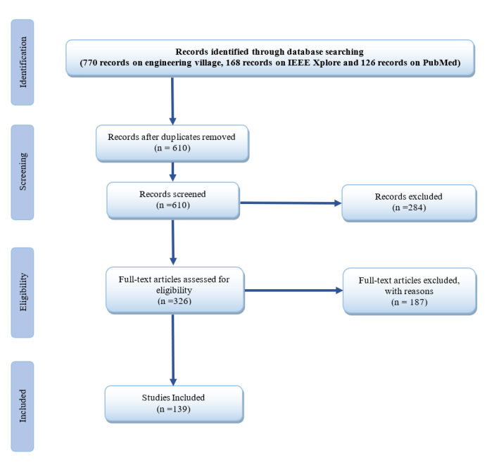
Figure 1: PRISMA systematic review diagram Dressel2017

1.2 Machine Learning Methodologies

Below is a brief overview of the key machine learning methodologies.

Supervised learning: This ML approach is used when the output is well defined. In this approach, the model is trained using labeled data to identify patterns and make predictions. Supervised learning can be divided into two categories, classification and regression. In classification, the model focuses on categorical predictions, while in regression, the model predicts continuous values. Popular supervised algorithms are logistic regression, linear regression, classification and regression trees (CART), Naive Bayes, neural networks, k-nearest neighbors (KNN) and support vector machines (SVM) chinnamgari2019r .

Unsupervised learning: This approach is used when the labeled data is unavailable. Unsupervised learning identifies patterns in the data to organize them. Unsupervised learning can be divided into clustering and association cios2007unsupervised . k-means, k-modes, hierarchical clustering, and fuzzy clustering are popular clustering algorithms in unsupervised learning.

Semi-supervised learning: This method combines both supervised and unsupervised approaches and requires a large amount of data to train the ML model. In applications such as medical imaging, where a large amount of unlabeled data are available, the semi-supervised approach uses the small amount of labeled data to build a model that can label the large dataset cios2007unsupervised ,chinnamgari2019r . Popular Semi-supervised learning methods are Generative adversarial networks (GANs), semi-supervised support vector machines (S3VMs), graph-based methods, and Markov chain methods.

Reinforcement learning: this method is distinct from both supervised and unsupervised learning. Reinforcement learning is based on a reward-based system in which an agent optimizes its actions based on the feedback it receives. Through this process, the algorithm learns optimal solutions to maximize cumulative rewards over time. Popular reinforcement learning algorithms are Q-learning, SARSA, deep Q network (DQN), and deep deterministic policy gradient (DDPG).

1.2.1 Machine Learning Algorithms

The following is a brief introduction to Machine learning algorithms:

Support Vector Machine (SVM): SVM is a supervised machine learning algorithm used for classification and regression tasks by constructing an optimal hyperplane that maximizes the margin between different classes Cortes1995 , Singh2016 . It is mainly effective in high-dimensional spaces and supports non-linear classification through kernel functions (e.g., Radial Basis Function (RBF), polynomial, sigmoid). Although SVM can handle high-dimensional feature spaces efficiently, performance may degrade if redundant or irrelevant features are included. Training SVM models, especially with non-linear kernels, can be computationally intensive due to quadratic programming complexity. The performance of SVM depends heavily on hyperparameter tuning, including the choice of kernel, regularization parameter CC, and kernel-specific parameters.

K-Nearest Neighbors (KNN): The KNN algorithm is a non-parametric, instance-based learning method used for classification and regression Zhang2016 . It classifies new samples by identifying the k nearest labeled data points and assigning the most frequent class among them (majority voting). Distance is typically measured using Euclidean distance. Since KNN does not construct an explicit model, it requires storing the entire dataset and performing real-time distance computations, making it computationally expensive for large datasets. KNN is sensitive to the presence of irrelevant or redundant features, which can distort distance calculations and degrade accuracy. Optimizations such as KD-Trees and Ball Trees can improve computational efficiency, particularly for high-dimensional data Zhang2016 .

Decision Trees: Decision trees are a widely used machine learning algorithm for classification and decision-making Podgorelec2002 . The algorithm systematically divides data into smaller subsets based on specific attribute values, forming a tree-like structure where internal nodes represent decision points and leaf nodes indicate final outcomes. One of the main strengths of decision trees is their simplicity, as they can handle both categorical and numerical data while offering a clear visual representation of decision processes. However, traditional algorithms can be prone to overfitting and may struggle with noisy or incomplete data.

Random Forests: Random Forest is an ensemble learning algorithm that enhances the predictive performance of individual decision trees by aggregating multiple tree models Au2018 . It operates using bootstrap aggregating (bagging), where multiple decision trees are trained on randomly sampled subsets of the data, reducing variance and mitigating overfitting. The method efficiently handles high-dimensional data, missing values, and both numerical and categorical predictors. However, categorical variables introduce challenges such as the ”absent levels” problem, where unseen categorical values at inference time can lead to undefined splits, impacting model robustness. Techniques such as surrogate splits and heuristics for missing data are used to mitigate this issue.

Logistic regression: Logistic regression is a statistical and machine learning model for binary classification Hosmer2013 ,Levy2020 . It estimates the probability of an outcome given a set of predictor variables by applying the logit function, ensuring that outputs remain between 0 and 1. The model is optimized using maximum likelihood estimation (MLE), and performance is typically assessed using goodness-of-fit tests, AUC-ROC, and classification metrics. While logistic regression assumes a linear relationship between predictors and log-odds, it can be extended with interaction terms or regularization techniques like LASSO and Ridge regression to improve generalization. Although machine learning models like random forests often outperform logistic regression in high-dimensional and complex datasets, logistic regression remains valuable for its interpretability and statistical inference capabilities.

Neural networks (NN): Neural Networks are computational models designed to recognize patterns and make predictions by mimicking the structure of biological neurons. They consist of interconnected layers: an input layer that receives raw data, hidden layers that extract features, and an output layer that produces the final result. Learning occurs through weight adjustments using optimization algorithms such as gradient descent, allowing NNs to generalize data Goodfellow-et-al-2016 . NNs have advantages such as adaptability to complex patterns, efficient feature learning, and scalability for large datasets. However, they require large datasets, significant computational power and are prone to overfitting without proper regularization.

Various types of NNs have different applications. Feedforward Neural Networks (FNNs) process data in one direction and are commonly used in classification and regression. Recurrent Neural Networks (RNNs) introduce feedback loops, making them suitable for sequential tasks like time-series prediction and speech recognition. However, traditional RNNs struggle with long-term dependencies, a challenge addressed by Long Short-Term Memory (LSTM) networks, which maintain memory over extended sequences mandic2001 .Convolutional Neural Networks (CNNs) are specialized for image and video processing, using convolutional layers to detect spatial patterns.

Autoencoders, composed of encoder-decoder structures, are useful for dimensionality reduction and anomaly detection. Generative Adversarial Networks (GANs) generate synthetic data by training two competing networks, finding applications in image synthesis and style transfer Goodfellow-et-al-2016 . Applications of NNs span multiple domains. FNNs are used in medical diagnosis and fraud detection, RNNs and LSTMs in speech recognition and financial forecasting, and CNNs in object detection and medical imaging. Autoencoders support data compression, while GANs enhance artificial content generation.mandic2001 , Goodfellow-et-al-2016 .

2 Review of algorithms to diagnose depression

2.1 EEG data acquisition

All studies in our systematic review have used an EEG dataset for their analysis. 102 of 139 (74. 38%) studies have collected their own EEG data, while only 20 research groups used a dataset that belonged to another study. The participant selection criteria varied between different research groups; 106 out of 139 (76. 25%) studies used a screening procedure to choose participants. The selection criteria for the choice of subjects were clinical interviews, questionnaires, and rating scales. 28 of 139 research studies did not mention the selection criteria they used to choose patients. 120 of 139 (86.33%) experiments were carried out in a controlled environment. Depending on the experiment in each research study, the EEG data was recorded while subjects were in the resting state with their eyes open or closed and with audio and visual stimulation. This is given in Tables 9 to 16. 12 of 139 research groups did not mention the condition of the experiment. The duration of the analysis was also significantly different in each study and ranged from 20 seconds to 34 minutes and in one experiment, from 9 to 10 hours. This was indicated by 118 of the 139 (84.89%) studies. 21 of 139 research studies did not provide any information on the analysis period. In this systematic review, the summary of the most recent literature based on the number and type of electrodes, their position, data acquisition device, sampling frequency, impedance and type of filters have also been provided in Tables 17 to 25. 96 of 139 (69. 06%) papers provided details of their data collection systems, while 43 of 139 papers did not mention any information about their data collection systems. 127 of 139 (91. 36%) papers mentioned the number of electrodes they used for their analysis. The minimum number of electrodes to collect data was 2 and the maximum number of electrodes was 128. In some of the papers, single electrode EEG diagnosis was studied, although the data was collected with a larger number of electrodes.

2.2 Preprocessing and feature extraction

Similar to many applications of EEG-based biomarkers, in most of the studies in our systematic review, preprocessing pipelines were implemented to remove artifacts from the EEG signal and denoise the signal. Of 139 papers, 43 studies (30.93%) have only used a bandpass filter, while 26 papers (18.7%) have used a combination of a bandpass and notch filter. 10 of 139 papers (7.19%) have also utilized a combination of low-pass, high-pass, and notch filter and 6 studies (4.31%) have only used low-pass and high-pass filter. Eight papers (5.7%) of studies have reported that only a notch filter has been used to remove powerline noise and its harmonies, and only one paper has used a combination of a high-pass and notch filter (0. 71%). 3 out of 139 studies (2.15%) have reported that a low pass filter has been used and another 2 studies have also mentioned the use of only a high pass filter. The authors of 4 out of 139 studies (2. 87%) have used a combination of wavelet filters, and another study has used a rectangular moving average filter. In addition, 2 studies have used a digital filter with cut-off frequencies of fc = 0.5 Hz and fc = 40 Hz, and another study has used median and band-stop filters. 27 out of 139 (19.42%) of the studies have not mentioned any traditional filtering stage namely Li2022 ,Garg2022 , Sharmila2022 , Lin2022 , Thakare2022 , Loh2021 , Hong2021 , Duan2021 , Zhu2020 , Saleque2020 , 8101151 , Liao2013 , 8981929 , Ke2019 , Mumtaz2019 , 19258582 ,18853691 , 20184806131498 , 20173504090707 , Wan2017AQA , Wan2017 ,17051427 , Frantzidis2012 , 20160801982396 , 20070710426068 , Pockberger1985 and 20185106271469 . One of the reasons that the authors have not reported the filtering characteristics is that in their experiments the filtering stage is integrated in their data acquisition system hardware. In addition to basic spectral filtering, more advanced artifact removals have also been utilized. Independent component analysis (ICA) was extensively used by several studies Movahed2022 , Zhao2022 , Kim2022 , Sun2022 , Babu2022 , Seal2022 , Ghiasi2021 , Movahed2021 , Li2021 , Sharma2021 , Uyulan2021 , Wang2021 , Seal2021 , Shen2021 , Duan2020 , Apsari2020 , Saleque2020 , Thoduparambil2020 , Mahato2020 , Mahato2020_2 , Kang2020 , 20193307311994 , 18951307 , 19258582 , 18927189 , 20183405723339 , 20185106271469 , 20183605764415 , XiaoweiLi2016EEG-basedClassifiers , Spyrou2016 , Frantzidis2012 , Ku2012 . Wavelet-based techniques have also been employed by several papers as a preprocessing algorithm to remove artifacts Song2022 , WeiEEGBASED2021 , Saeedi2020 , 19203658 , 18853691 , Cai2018ACASE , Cai2018ADetection , Wan2017AQA , Shen2017ACriterion , Zhao2017 , Wan2017 , Cai2017NO2 , Puthankattil2017 , Cai2016PervasiveCollector . Most of the papers extracted linear and non-linear features from their dataset and created a feature space for further analysis. A short description of the type of features has been mentioned, and further details of the features are shown in Tables 26 to 28.

2.3 Data processing and machine learning

In this section, we report a summary of each article based on machine learning algorithms and statistical analysis utilized. Some of the authors have used a combination of different data processing techniques and concluded that one of them had achieved the highest performance metrics. This is mentioned in Tables 2 to 8. In addition, performance metrics (accuracy, specificity and sensitivity) of the techniques have also been reported in Tables 2 to 8. Some of the authors have not reported performance metrics or only reported the accuracy of the results in their articles. This is reported as N/A in the tables. In the next section, we have categorized the papers with highest accuracy based on the data processing technique and the machine learning approach that they have used.

2.3.1 Logistic Regression

16 out of 139 papers (11.51%) of papers we studied used logistic regression in their analysis. Hosseinifard et al. Hosseinifard2013 explored a nonlinear method to characterize depressed and healthy subjects. In their study, they used EEG signals from 19 channels located on prefrontal, frontal, parietal, central, temporal and occipital lobes to extract non-linear and linear features, including Lyapunov exponent (LE), correlation dimension, Higuchi fractal (HF), and band powers. The authors also employed detrended fluctuation analysis (DFA) to calculate correlation properties and fractal scaling of the EEG signal. Features were selected using GA. LR, LDA, and KNN classifiers were used to classify features. Among linear features, Alpha band power and among nonlinear features, correlation dimension showed highest accuracy to discriminate patients. The results show that Logistic Regression (LR) classifier can achieve higher accuracy in comparison to KNN and LDA. In a study by W. Mumtaz et al. Mumtaz2015ADisorder , the authors used the choice of three EEG references using LR and SVM to discriminate patients with depression from healthy controls. 33 depressed and 19 healthy subjects participated in their study. The EEG signal was collected from 19 electrodes using BrainMaster 24 E amplifier (BrainMaster Technologies, Inc., USA) at the sampling frequency of 256 Hz. The EEG data was denoised with Surrogate filtering technique. Inter-hemispheric asymmetries, Power of different EEG frequency bands and coherenc were exracted from the signal. The authors studied three EEG references of average reference (AR), infinity reference (IR), and link-ear (LE) reference and achieved the highest accuracy, specificity, and sensitivity with LR. In addition to above papers, authors in Babu2022 , Jan2022 , Li2021 , Jiang2021 , Hong2021 , WeiEEGBASED2021 , Duan2021 , Saleque2020 , Sun2020 , Mahato2020_2 , Ding2019 , Cai2018StudyFS and Li2015Second have also used Logistic Regression in their studies.

2.3.2 Support vector machine (SVM)

In our systematic review, 53 out of 139 papers (38.12%) used the SVM classification algorithm to classify depressed patients from healthy control subjects. I. Kalatzis et al. 8101151 were one of the first research groups to use SVM with the Majority-Vote engine to identify patients with depression. In their study, 25 depressed and 25 healthy subjects were selected. The authors used audio stimulation to collect resting-state EEG data from 15 Ag/AgCl electrodes at the sampling frequency of 500 Hz. 17 features were extracted from EEG signal and the authors achieved the maximum classification accuracy with all the leads. During specific tasks, right brain hemisphere dysfunction was observed in depressed group. T.Tekin Erguzel et al. TekinErguzel2015 proposed an algorithm based on Ant Colony Optimization (ACO) and SVM. EEG data were collected from 55 patients with mild depression and 46 patients with bipolar disorder. Neuroscan EEG cap (Compumedics, NC, USA) with 19 Ag/AgCl electrodes were used to collect EEG data at the sampling frequency of 250Hz. The authors proposed an Improved ACO technique to select 22 of 48 features. In their research, they achieved the highest performance metrics with the IACO-SVM algorithm. The authors calculated the Area under curve (AUC) of 0.793. Using nested cross-validation (CV), it was shown that the accuracy of the proposed algorithm was higher than Particle swarm optimization (PSO), Genetic algorithm (GA), and ACO algorithm. K. M. Puk et al. Puk2016 explored a technique to discriminate depressed and healthy subjects based on the effects of depression on memory processing. 15 depressed and 12 normal subjects participated in the study, and EEG data were collected with a 32 channel Brain vision system from (Brain products GmbH, Germany) at a sampling frequency of 1000Hz. In order to reduce the size of the dataset, the signal was resampled to 256Hz, and 9 groups of linear and nonlinear features were extracted from the signal. In order to select features with the highest discriminative properties, the Minimal-Redundancy Maximal-Relevance criterion (mRMR) technique was employed. The selected features were classified with the SVM classifier, and the classification accuracies of over 80% were achieved. In another study by J. Shen et al. Shen2017ACriterion , a method was developed by the authors to diagnose depression with three Fp1, Fp2, and FpZ electrodes. EEG data were collected from 81 Depressed and 89 healthy subjects with a Three-electrode pervasive EEG collection device (Ubiquitous Awareness and Intelligent Solutions (UAIS), Lanzhou University, China) at the sampling frequency of 250Hz. Ocular artifacts were removed by Discrete wavelet transform (DWT) and Kalman filter. Three linear features of Centroid frequency, Mean frequency and Max frequency and three nonlinear features of C0 complexity, Correlation dimension and Renyi entropy were extracted from five EEG frequency bands: Alpha (8-13 Hz), Beta (13-30Hz), Theta (4-8 Hz), Delta (1-4 Hz) and Full band (1-40Hz). The authors used SVM to discriminate depressed and healthy subjects. W. Mumtaz et al. 20172903942647 proposed a machine learning algorithm based on Synchronization likelihood (SL) to discriminate depressed and healthy subjects. In this study, EEG data were collected from 34 depressed and 30 control subjects using 19 electrode EEG cap with a BrainMaster Systems amplifier (BrainMaster technologies Inc., USA) at sampling frequency of 256Hz. The authors used the Multiple Source technique to remove artifacts. A feature matrix was created for each subject, and a rank-based algorithm was used to select relevant features. Selected features were classified with 10-fold cross-validation with Logistic Regression (LR), SVM, and Naive Bayesian (NB) classifiers. The highest performance metrics was achieved with SVM classifier. The authors claimed that the 95% specificity of the proposed method shows that the algorithm can potentially be used in clinical setting. I. Spyrou et al. Spyrou2016 studied neurophysiological features of 34 patients with Geriatric depression and neurodegeneration with 32 healthy subjects to discriminate between the two groups. A Nihon Kohden JE-207A (Nihon Kohden Europe GmbH) data acquisition system was used to collect EEG data. The subjects asked to wear a 57 electrode cap (EASYCAP from EasyCap GmbH) and data was collected at sampling frequency of 500Hz. In their approach, they extracted oscillatory and synchronization features based on Discrete wavelet transform (DWT). The authors employed the Random Forest (RF), Random Tree (RT), SVM and Multilayer Perceptron (MLP) classifiers to calculate the accuracy of their method. They achieved the highest classification accuracy, specificity and sensitivity with the RF classifier. S. Mantri et al. 15670461 used EEG linear analysis and SVM classifiers to discriminate 13 depressed and 12 control subjects. EEG signals were captured with an 8-channel data acquisition device with F3, F4, Fz, C3, C4, Pz, P3, and P4 electrodes which are located at Frontal, Occipital and Parietal lobes. The sampling frequency of 256 Hz was used for data acquisition. The power spectrum of four different bands was calculated, and the extracted features were classified with SVM classifier. The results showed that the proposed SVM classifier can be utilized to achieve the highest performance metrics. X. Li et al 20193307311994 studied the reliability of EEG machine learning analysis based on emotional face stimulation task to discriminate depressed and healthy subjects. 14 depressed and 14 healthy subjects participated in the experiment. The authors used a 128 electrode HydroCel Geodesic Sensor Net (Electrical Geodesics, Inc., USA) with 250 Hz sampling frequency to collect EEG data. 16 electrodes located on prefrontal, frontal, central, temporal, parietal and occipital lobes were selected for analysis. FastICA algorithm and an adaptive noise canceller based on LMS algorithm were employed to remove artifacts. Power spectral density and activity and Hjorth features were extracted from the EEG data and the authors employed an ensemble method based on deep forest and SVM. The best performance metrics were achieved with ensemble model and power spectral density. In another study by S.C. Liao et al Liao2017 , an a new feature extraction method based on spectral-spatial EEG features was proposed to discriminate depressed and healthy subjects based on. 12 depressed and 12 healthy subjects were participated in the experiment. EEG data was collected from 30 Ag/AgCl electrodes with a Quick-Cap 32 EEG data acquisition device at 500 Hz sampling frequency. The ocular artifacts were removed by NeuroScan artifact removal software. Theta (4–8 Hz), alpha (8–13 Hz), beta (13–30 Hz) and gamma (30–44 Hz) band powers and correlation dimension were extracted from the EEG signal. The highest performance achieved with the combination of kernel eigen-filter-bank common spatial pattern (KEFB-CSP) feature extraction method proposed by authors and SVM classifier. The authors achieved the highest accuracy, specificity and sensitivity of with 8 electrodes and 6 seconds of recorded EEG data. Authors in Mumtaz2017 proposed a machine learning platform to discriminate depressed patients and healthy subjects. The researchers collected EEG data from 33 depressed and 33 healthy subjects. To collect data, they used 19-channels EEG cap with BrainMaster Systems amplifier (BrainMaster technologies Inc., USA) at the sampling frequency of 256 Hz. The electrodes were located on frontal, temporal, parietal and occipital lobes. Multiple source techniques with standard brain electric source analysis (BESA) software was used to remove artifacts and alpha interhemispheric asymmetry and EEG spectral power features were extracted from EEG data. The proposed machine learning platform achieved the highest performance metrics with SVM classifier. In another study by M. Sharma et al. 18983501 , the authors proposed a method to diagnose depression based on three-channel orthogonal wavelet filter bank (TCOWFB). 15 depressed and 15 healthy participated in the study. The EEG data was collected from Bipolar channels FP2-T4 (right half) and Fp1-T3 (left half) at 256 Hz sampling frequency. Ocular and muscle artifacts were manually removed with visual inspection and nonlinear features were extracted from seven wavelet sub-bands. The authors concluded their method has lower computational complexity and higher performance in comparison to previous studies. In addition to the mentioned papers, authors of other papers including Li2022 , Zhao2022 , Kim2022 , Zhang2022 , Lin2022 , Avots2022 , Sun2022 , Nayad2022 , Babu2022 , Jan2022 , Seal2022 , Ghiasi2021 , Movahed2021 , Movahed2021 , Li2021 , Sharma2021 , Jiang2021 , Hong2021 , WeiEEGBASED2021 , 9477800 , Shen2021 , Duan2021 , Saeedi2020 , Duan2020 , Saleque2020 , Mahato2020 , Mahato2020_2 , Ding2019 , Cai2018StudyFS , Li2015Second , Orgo2017 , 17991812 , 20193407357198 , also used SVM algorithm in their studies. Details of the utilized techniques are provided in Tables 2 to 8.

2.3.3 K-Nearest Neighbor (KNN)

In addition to the SVM classifier, 25 out of 139 papers (17.98%) of papers have used the KNN classifier in their studies. X. Li et al. 15798207 proposed an algorithm using linear and nonlinear features with the KNN classifier. EEG data was collected from 9 depressed and 25 control subjects with a 128 channel Geodesic sensor net (Electrical Geodesics, Inc., USA). The sampling frequency was set to 250HZ. 20 linear and nonlinear features including sum power, max power, variance, Co-complexity, Lyapunov, and Kolmogorov entropy were extracted from delta (0.5–4Hz), theta (4–8Hz), alpha (8–13Hz) and beta (13–30Hz) frequency bands. The researchers implemented methods based on KNN, SVM, LR, NB and RF classifiers. The authors achieved the classification accuracy of over 99% based on KNN classifier with the combination of linear and nonlinear features. In another study by X. Zhang et al. 13386381 , the authors proposed an approach to characterize depressed and healthy females with three electrodes (Fp1, Fp2, and FpZ) on prefrontal lobe. The researchers developed a 3-electrode mobile EEG belt for EEG data acquisition and collected data at the sampling frequency of 256 Hz. In their method, several linear and nonlinear features were extracted from 13 depressed and 12 healthy subjects. KNN, and Backpropagation neural network (BPNN) classifiers were used to classify depressed and control subjects. In their study, the authors achieved higher classification accuracy with BPNN in comparison to KNN. X. Li et al. XiaoweiLi2016EEG-basedClassifiers proposed an algorithm based on Greedy Stepwise (GSW) and KNNs to discriminate patients with mild depression and healthy subjects. The authors used a 128 channel HydroCel Geodesic Sensor Net (Electrical Geodesics, Inc., USA) at the Sampling frequency of 250 Hz to collect data from 10 depressed and 10 control subjects. Eight linear and 9 non-linear features were extracted, and five feature selection methods of Greedy Stepwise, Best First (BF), Linear Forward Selection (LFS), Genetic Search (GS), and RankSearch (RS) were used for data dimensionality reduction. The authors achieved the highest classification accuracy with the GSW-KNN algorithm using 16 electrodes. It was concluded that five electrodes of T3, O2, Fp1, Fp2, and F3 which are located on temporal, occipital, prefrontal and frontal lobes could achieve high performance metrics. S. Zhao et al. Zhao2017 designed a real-time system to monitor and discriminate depressed patients and control subjects. The EEG data were collected with three Fp1, Fp2, and FpZ electrodes which are located on prefrontal lobe at the sampling rate of 256Hz with an audio stimulus. The authors used a Finite impulse response (FIR) filter, a mid-filter, Wavelet transforms, and Kalman filter to remove noise. Three linear features of Max frequency, Mean Frequency, and Center Frequency in combination with three non-linear features of C0 Complexity, Permutation Entropy and Lempel Ziv complexity (LZC) were extracted from the signal. The proposed algorithm using six extracted features achieved and average classification accuracy of over 78% with Local classification based on KNN and Naïve Bayes. H. Cai et al. Cai2018ADetection explored the feasibility of developing an algorithm to differentiate depressed patients with three electrodes. The authors collected data from 92 depressed and 121 control subjects with data acquisition device (Ubiquitous Awareness and Intelligent Solutions (UAIS), Lanzhou University, China) using three electrodes of Fp1, Fp2, and FpZ at the sampling frequency of 250 Samples per second. To denoise the signal, the authors used DWT, Adaptive predictor filter (APF) and FIR filters. Two hundred seventy linear and nonlinear features were extracted from the signal, and the authors used the Minimal-Redundancy-Maximal-Relevance algorithm to select relevant features from the feature matrix. The highest classification accuracy was achieved with KNN. It was concluded that the absolute power of theta could be a significant indicator to discriminate depressed and healthy controls. In another study by H. Cai et al. Cai2018ACASE , the authors proposed a new method based on normalized Euclidean distance to increase the accuracy of the previous algorithm. 86 depressed and 92 healthy subjects were participated in the study and data was collected from three Fp1, Fp2, and FpZ electrodes on prefrontal lobe with a data acquisition device (Ubiquitous Awareness and Intelligent Solutions (UAIS), Lanzhou University, China) at the sampling frequency of 250 Hz. Wavelet transform was used to remove signal artifacts and a combination of linear and nonlinear features were extracted. The authors achieved the highest accuracy with the KNN classifier with the proposed method. In addition to the selected papers summarized in the above, authors in Kim2022 , Zhang2022 , Avots2022 , Nayad2022 , Babu2022 , Seal2022 , Li2021 , Jiang2021 , WeiEEGBASED2021 , 9477800 , Saeedi2020 , Duan2020 , Sun2020 , Cai2018StudyFS , Li2015Second and 19203658 have also used KNN classifier as mentioned Tables 2 to 8..

2.3.4 Neural Networks

44 out of 138 papers (31.65%) of papers we studied used neural networks in their analysis. S. D. Puthankattil et al. Puthankattil2012ClassificationEntropy employed Relative Wavelet Energy (RWE) and Artificial Neural Network (ANN) classifiers to discriminate 30 healthy and 30 depressed subjects. They used Fp1-T3 and Fp2-T4 electrodes to collect EEG data at the sampling frequency of 256 Hz. In their study, Ocular and muscle artifacts were manually removed, and Total Variation Filtering (TVF) were employed to denoise the signal. They found the signal energy distribution can be used to characterize depressed and control subjects. Y. Katyal et al. Katyal2014 proposed an algorithm based on the combination of EEG signal and facial emotion analysis. In their study, 10 healthy and 10 depressed subjects were participated. The data was collected with 64 EEG electrodes at the sampling frequency of 256 Hz. They used ICA to eliminate artifacts and Wavelet packet decomposition (WPD) was employed to extract features from EEG data. To classify features from EEG signals and facial recognition analysis, the authors proposed a classifier based on the ANN. The authors concluded they could achieve higher accuracy by combining EEG analysis and facial recognition. T. Erguzel et al. Erguzel2016 proposed an approach based on cordance values (which is calculated based on quantitative electroencephalographic (QEEG)), PSO and ANN. The EEG data were collected from 31 bipolar and 58 unipolar subjects with 19 Ag/AgCl electrodes using Scan LT EEG Amplifier (Compumedics/Neuroscan, USA) with an EEG cap at the sampling frequency of 250 Hz. The authors then used normalized absolute and relative powers of each electrode to calculate cordance values for each frequency band. PSO evolutionary computation algorithm was used to select features from the feature matrix. The proposed approach based on hybrid PSO and ANN achieved the highest performance metrics. Y. Mohan et al. Mohan2016 presented an algorithm based on ANN to classify two groups of 5 depressed and 5 control subjects. Data was collected with a 32 wet electrode data acquisition device at the sampling frequency of 128Hz. A multilayer feed-forward network was used to classify data using 800 input neurons per electrodes. The authors concluded that C3 and C4 electrodes in the central part of the brain can be utilized to classify depressed and healthy subjects with high accuracy. H. Cai et al. Cai2016PervasiveCollector studied the feasibility of a portable EEG system to discriminate depressed and healthy subjects based on Deep Belief Networks (DBN). 86 depressed and 92 control subjects participated in the experiment. The researchers used a Three-Electrode Pervasive EEG Collector (Ubiquitous Awareness and Intelligent Solutions (UAIS), Lanzhou University, China). The electrodes were Fp1, Fp2, and FpZ, which are located on the prefrontal cortex. 28 linear and nonlinear features were extracted and KNN, SVM, ANN and DBN were employed to analyze features and find features with the highest discriminative power. The results indicate that DBN and the absolute power of Beta wave (13-30Hz) can achieve the highest accuracy. S. D. Puthankattil et al. Puthankattil2017 studied the Probabilistic Neural Network (PNN) and Feedforward Neural Network (FFNN) methods to discriminate depressed and healthy subjects. EEG data were collected from 30 depressed and 30 control subjects with a 24-channel data acquisition system at 256Hz sampling frequency. The authors used DWT to decompose the signal and extracted time-domain features. In addition, RWE and wavelet entropy (WE) were also calculated. The authors achieved highest classification accuracies with RWE-FFNN and WE-FFNN respectively. It was concluded the proposed algorithm based on time and domain features with FFNN could achieve higher classification accuracy compared to other classifiers. U. Acharya et al. Acharya2018AutomatedNetwork proposed a technique to classify depressed and healthy subjects based on Convolutional Neural Network (CNN). The proposed algorithm can discriminate patients and healthy controls without using a feature matrix. The authors used Fp1-T3 and Fp2-T4 channel pairs to collect data from 15 depressed and 15 healthy subjects at the sampling frequency of 256Hz. It was concluded that the right hemisphere EEG signals could achieve higher classification accuracies compared to left hemisphere EEG signals. Y. Guo et al. 20173504090707 proposed a classification function based on linear discriminant analysis (LDA) and a new algorithm based on the Multi-Objective Particle Swarm Optimization (MOPSO) algorithm to discriminate depressed and healthy subjects. The authors used a 14-electrode data acquisition system with Emotive headset (Emotive Inc., USA) at 128 SPS (samples per second) to collect EEG data from 3 depressed and 3 healthy subjects. The authors used AF3, AF4, F3, F4, F7, F8, FC5, FC6, T7, T8, P7, P8, O1 and O2 electrodes to collect data. LDA and MOPSO classification results achieved the highest performance metrics with 6 volunteers. H. Cai et al. Cai2017NO2 studied depression diagnosis based on gender differences in a group of 90 depressed and 68 healthy subjects. A Three-electrode EEG collector (Ubiquitous Awareness and Intelligent Solutions (UAIS), Lanzhou University, China) was used to collect EEG data. Two electrodes of Fp1 and Fp2 which are located on prefrontal lobe were selected for further analysis and ocular, muscle and powerline artifacts were removed by a bandpass filter and wavelet transform. The authors extracted 32 linear and nonlinear features from the signal and employed the Sequential Floating Forward Selection (SFFS) algorithm and SVM, KNN, DT and ANN classifiers to find the most effective features to discriminate depressed and healthy subjects. The highest classification accuracy to discriminate male subjects achieved with ANN classifier while for female subjects the highest classification accuracy observed with KNN. It was concluded that for male subjects the best results achieved under resting state and females, the highest classification accuracy was obtained under negative audio stimulation. P. Sandheep et al. Sandheep2019 proposed a machine learning approach based on CNN to distinguish depressed and healthy subjects. 30 depressed and 30 healthy subjects were selected for the experiment and EEG data was collected from Left half (Fp1-T3) and right half (Fp2-T4) of the brain at 256Hz sampling frequency. After z-score normalization to normalize data, the authors employed a five-layer CNN. The results showed that the classification accuracy was higher in the right-brain hemisphere in comparison to left-brain hemisphere. The researchers concluded that with their proposed five-layer CNN platform and without using a feature extraction algorithm, high performance metrics to discriminate depressed and healthy subjects is achievable. In another study by W. Mumtaz et al. Mumtaz2019 , two deep learning depression diagnosis frameworks based on One dimensional CNN (1DCNN) and 1DCNN with long short-term memory (LSTM) were proposed. 33 Depressed and 30 Healthy subjects participated in the study and EEG data was collected from 19 channels at the sampling frequency of 256 Hz. To eliminate ocular artifacts, multiple source eye correction (MSEC) algorithm was employed. The highest performance metrics were achieved with 1DCNN model and 1DCNN with LSTM model respectively. It was concluded that the proposed 1DCNN models can be used in developing wearable systems due to low complexity and high performance of the models. S. Mahato et al. 20183405723339 explored linear, nonlinear and combination of features to distinguish depressed and healthy subjects. The authors selected 34 depressed 30 healthy for the experiment and using 19 electrodes they collected EEG data from frontal, temporal, parietal, occipital and central lobes of subjects at the sampling frequency of 256 Hz. ICA and common average reference (CAR) were employed to remove signal artifacts. Band power (delta (0.5–4 Hz), theta (4–8 Hz), alpha (8–13 Hz) and beta (13–30 Hz)) and Interhemispheric asymmetry linear features were extracted. In addition, nonlinear features of Wavelet transform, Relative wavelet energy (RWE) and Wavelet entropy (WE) were also extracted from the EEG signal. The researchers employed Principal component analysis (PCA) algorithm as a dimension reduction algorithm to reduce the number of irrelevant features. The EEG data was analyzed using Multi-layered perceptron neural network (MLPNN), radial basis function network (RBFN), LDA and quadratic discriminant analysis (QDA). The highest classification accuracy, specificity, and sensitivity was achieved with the combination of alpha power and RWE features with MLPNN and RBFN classifiers. In another study by H. Ke et al. 20184806131498 , The authors proposed a cloud-based machine learning framework for wearable systems using a light weight CNN. The authors collected EEG data from three groups of healthy and pressed subjects. Dataset 1 consists of 34 depressed and 30 healthy subjects and dataset 2 consists of 17 depressed patients. The data was collected with 20 electrodes located on prefrontal, frontal, temporal, central, parietal and occipital lobes at the sampling frequency of 256 Hz. The proposed light weight CNN achieved classification accuracy of over 98. It was concluded that the proposed machine learning framework is suitable for use in wearable healthcare application due to high performance, fast processing time and low computational complexity. O. Faust et al. Faust2014 proposed a PNN machine learning framework for depression treatment and diagnosis. The authors chose 30 depressed and 30 healthy subjects for their experiment and collected EEG data from Fp1-T3 (left half of brain) and FP2-T4 (right half of brain) at the sampling frequency of 256 Hz. Artifacts were removed by TVF algorithm and visual inspection. A combination of linear features of Wavelet packet decomposition and nonlinear features of Bispectral phase entropy, Renyi entropy, Sample entropy and Approximate entropy were extracted from the EEG signal. Student’s t-test was employed to select discriminative features and different classifiers such as KNN, SVM, DT, NB, Gaussian mixture model (GMM), Fuzzy Sugeno Classifier (FSC) and PNN were utilized to calculate the performance metrics. The authors achieved the highest performance metrics with PNN. In addition to the selected papers summarized above, other articles Wang2DCNN2022 , Sharmila2022 , Zhang2022 , Song2022 , Wang2022 , Nayad2022 , Goswami2022 , Jan2022 , Seal2022 , Thakare2022 , Loh2021 , Savinov2021 , Uyulan2021 , Seal2021 , Duan2020 , Thoduparambil2020 , Kang2020 , 8981929 , 18768750 , 19259295 , Ke2019 , 18951307 , 19258582 , 18927189 , 20185106271469 , 20194907787800 also used Neural networks in their research, as shown in Tables 2 to 8.

2.3.5 Statistical Analysis

31 out of 139 papers (22.30%) in our systematic review have used statistical analysis to discriminate depressed patients and healthy subjects. The authors in 20102413002260 studied Spectral Asymmetry (SA) with Mann-Whitney U-test and Bonferroni Correction on 18 Depressed and 18 Healthy female subjects. They collected EEG data with Cadwell Easy II (Cadwell Industries Inc., USA) EEG data acquisition system at the sampling frequency of 400 Hz. 19 electrodes located on frontal, parietal, temporal and occipital lobes were used during the experiment. Power spectral density (PSD), EEG band Powers and SA features were extracted from the EEG signal. Their results show that the proposed technique can distinguish depressed and control subjects based on SA and confirm higher relative beta and beta power in depressed patients in all the areas of the scalp. Authors in 12424821 explored cortical functional connectivity of 12 depressed and 12 healthy subjects by using a method of partial directed coherence (PDC). In their research, they used a 16-channel data acquisition system (Sunray, LQWY-N, Guangzhou, China) with 100Hz sampling frequency. They placed the electrodes on prefrontal, frontal, central, parietal, occipital and temporal regions of brain. The authors removed the artificats manually. One-way ANOVA statistical analysis showed the presence of Hemispheric Asymmetric Syndrome in depressed patients. M. Bachmann et al. Bachmann2015 studied the complexity of EEG signals using Lempel Ziv Complexity method. They used an 18 channel Cadwell Easy II (Cadwell Industries Inc., USA) EEG data acquisition system with 400Hz sampling frequency to collect EEG data from 17 depressed and 17 control subjects. Electrodes were located on prefrontal, frontal, central, parietal, temporal and occipital lobes. Mann-Whitney statistical test showed a significant difference in the complexity of the algorithm between two groups. Z.Liao et al. Liao2013 studied correlation and Asymmetry analysis on 10 healthy, 7 unmedicated, and 5 medicated depressed patients taking antidepressant. They used six forehead and parietal electrodes (Fp1, Fp2, F3, F4, P3, and P4) with the Brain Vision Recorder (Brain products GmbH, Germany) at the sampling frequency of 500 Hz. To remove artifacts, the authors used Brain Vision Recorder (Brain products GmbH, Germany) and Analyzer Filter. The proposed method proved the correlation between the beta frequency band in the frontal brain area and the (Beck Depression Inventory) BDI score. M. Sun et al. Sun2015 studied the power spectral analysis to categorize depressed and healthy patients. The authors collected EEG data from 11 healthy and 11 depressed patients with three prefrontal electrodes (FP1, Fp2 and FpZ) at the sampling frequency of 256Hz. Gravity frequency of power spectrum and relative power features were extracted from the signal. The Results from statistical analysis showed depressed patients have lower relative power in the alpha band (8-14Hz) and higher relative power in the beta band (14-30Hz). D. P. X Kan et al. 20161302158441 studied the alpha-1 (8-10 Hz) and alpha-2 (10-12 Hz) waves as biomarkers to discriminate depressed and healthy subjects. The authors collected EEG data from 4 depressed and 4 control subjects using an NCC Medical data acquisition device (NCC Medical Co. Ltd., China) with 32 channels. In this research, mean absolute spectral values were extracted from alpha1 (8-10 Hz) and alpha2 (10-12 Hz) bands in two conditions of eyes closed and eyes open. The Paired T-Test statistical analysis showed lower-alpha (8-10Hz) waves in the depressed group in T5, T6, O1, O2, P3, and P4 electrodes which are located on temporal, occipital and parietal lobes. K. Kalev et al. Kalev2015 examined Multiscale Lempel Ziv Complexity (MLZC) to exceed the accuracy of traditional LZC in discriminating depressed and control subjects. In their research, the authors collected data from 11 depressed and 11 control subjects using the Neuroscan Synamps2 (Compumedics, NC, USA) data acquisition system at the sampling frequency of 1000 Hz, which was later downsampled to 200Hz. To differentiate depressed and control subjects, the authors used the Wilcoxon Rank-Sum statistical test. The classification accuracy in LZC and MLZC was calculated with LDA and is shown in Table 1. The highest classification accuracy was achieved with channel F3 and It was concluded that MLZC could significantly increase the classification accuracy compared to traditional LZC.

Table 1: Classification accuracy of LZC and MLZC from Kalev2015

Channel Classification Accuracy Corresponding Frequency F3 86.36% 9Hz and 15.5Hz F7 81.82% 28.5Hz and 40Hz Fp1 77.27% 2-6Hz, 9Hz, 10Hz and 12Hz

S. Akdemir Akar et al. 15605052 evaluated the nonlinear analysis of EEG to differentiate depressed and control subjects. The authors used a BrainAmp DC acquisition system (Brain products GmbH, Germany) at the sampling frequency of 250Hz to collect EEG data from 15 depressed and 15 healthy subjects. The electrodes were located on prefrontal, frontal, central, parietal and temporal lobes and the ocular artifacts were removed both by data acquisition system and by visual inspection. Higuchi’s fractal Dimension (HFD), Shannon entropy, Lempel-Ziv complexity, Katz’s fractal dimension (KFD), and Kolmogorov Complexity features were extracted. The Analysis of variance (ANOVA) showed LZC, HFD, and KFD values can discriminate depressed and control subjects with higher accuracy compared to Kolmogorov complexity (KC) and Shannon entropy (ShEn) values. In another study by S. A. Akar et al. 20160201780626 , the authors studied the wavelet analysis combined with KFD and HFD to discriminate depressed and healthy patients. The EEG data were collected from 16 depressed and 15 healthy subjects with a Brain-Amp DC acquisition system (Brain products GmbH, Germany) at 250Hz sampling frequency. The authors used Fp1, Fp2, F3, F4, F7, F8, P3, P4, P7, and P8 electrodes which are located on prefrontal, frontal and parietal lobes. Artifactes were removed by visual inspection. Fractality analysis and ANOVA statistical analysis shows that KFD and HFD values can be used to distinguish patients and healthy subjects. A. Frantzidis et al. Frantzidis2012 explored a method with a DWT and Mahalanobis Distance (MD) classifier. A group of 33 depressed and 33 control subjects participated in their study. To collect EEG data, they used the Nihon Kohden JE-207A (NIHON KOHDEN EUROPE GmbH) device with 57 electrodes. Signal artifacts were removed by ICA and visual inspection. Their results showed significant variation in the delta band (0.5-4 Hz) between depressed and healthy groups. Z. Wan et al. Wan2017 proposed an algorithm to classify patients based on EEG and Patient’s Clinical self-rating data. The self-rating emotional data used in the study is collected for two weeks by patients using an electronic self-rating scale called Profile of Mood Status and Brief Chinese Norm (POMS-BCN). The authors used a B3 EEG band (Neuro-Bridge, Japan) with a NeuroSky EEG sensor (NeuroSky, Inc.) at the sampling frequency of 512Hz to collect EEG data from 5 patients. First, Principle Component (FPC) curve was calculated based on PCA from clinical self-rating data collected by users. The signal was denoised and decomposed with DWT, and a feature vector was created with 256 features extracted from 5 EEG bands. The authors used the RF algorithm for further analysis and built a quantization model. The results showed that the proposed algorithm could compute mood statues with a high correlation with self-rating values. A. Suhhova et al. Suhhova2013 explored individual and traditional fixed EEG frequency bands using the Spectral Asymmetry Index (SASI) on two groups of 18 depressed and 18 control subjects. They collected EEG data from 19 electrode Cadwell Easy II (Cadwell Industries Inc., USA) data acquisition system at the sampling frequency of 400 Hz. The authors chose parietal P3 electrode for analysis. Power spectral density and EEG signal power features were extracted from the EEG data. Their results show that individual SASI analysis is more consistent than traditional fixed SASI to differentiate depressed and healthy subjects. M. Bachmann et al. Bachmann2017 investigated single-channel EEG analysis based on DFA and SASI to discriminate depressed and healthy subjects. The authors used an 18 channel Cadwell Easy II (Cadwell Industries Inc., USA) EEG data acquisition system at the sampling frequency of 400 Hz to collect data from 17 depressed and 17 control subjects. LDA was employed to classify two groups and compute accuracy, specificity, and sensitivity. The highest performance metrics was achieved with combined SASI and DFA algorithms. It was also concluded that Pz electrode which is at Parietal lobe has the highest accuracy in discriminating two groups. W. Mumtaz et al. Mumtaz2015-NO2 used DFA and LR with 10-fold cross-validation to discriminate depressed and healthy subjects. In their study, EEG data were collected from 33 depressed and 33 control subjects using 19 of 24 channels with an EEG data acquisition device with BrainMaster 24 E amplifier (BrainMaster technologies Inc., USA) at the sampling frequency of 256Hz. The electrodes were placed on prefrontal, frontal, central, temporal, parietal and occipital lobes. The authors used DFA combined with three approaches to extract and select features. T-test, Wilcoxon, and Receiver Operating Characteristics (ROC) were used to rank features. The algorithm was also used with three EEG referencing methods: IR, AR and LE. The highest performance was achieved by AR with t-test. The authors concluded that the proposed algorithm could be used to discriminate healthy and depressed patients. M. Bachmann et al. Bachmann2018 explored different methods for single channel depression diagnosis. The EEG data was collected from 13 depressed and 13 healthy participants with 30 electrodes based on International 10/20 extended system. A Neuroscan Synamps2 (Compumedics, NC, USA) was used for EEG data acquisition at the sampling frequency of 1000 Hz. The signal was visually inspected, and artifacts were removed. A combination of linear features of Alpha power variability, Relative gamma power and Spectral asymmetry index were extracted from the signal. In addition, nonlinear features of Detrended fluctuation, HFD and Lempel-ziv complexity were extracted from the signal. To measure the difference between two groups of depressed and healthy subjects, the authors used Mann-Whitney statistical test. LR classifier with leave-one-out cross-validation was also employed to classify data. The authors achieved the highest classification accuracy with the combination of linear and nonlinear features from a single channel located on central lobe. In another study by W. Mumtaz et al. Mumtaz2016 , The authors proposed a machine learning framework to discriminate depressed and healthy subjects based on features extracted from Event-related potentials (ERP). 29 depressed and 15 healthy subjects were participated in the study and EEG data was collected with 19 wet electrodes using BrainMaster Discovery amplifier (BrainMaster technologies Inc., USA) at 256 Hz sampling frequency. Ocular and muscle artifacts were removed by Surrogate filtering method with BESA. ERP features were extracted the signal and a large dataset was created. To reduce the number of irrelevant features, three feature selection criteria of T-test, Wilcoxon and ROC were employed. The authors achieved the highest classification accuracy with Fz and with Pz located on central regions of brain. It was concluded that it is feasible to discriminate depressed and healthy subjects with single channel EEG analysis using ERP features. In addition to the selected papers summarized in the above, other papers, including Orgo2017-NO2 , Li2016 , Zhao2013 , Suhhova2009 , Pockberger1985 , Lee2007 , Li2007 , Li2015 , Wan2017AQA , Hinrikus2009 , 20190906547554 , and 18853691 have also used statistical analysis in their research. In addition, functional connectivity and coherence have been used by Peng2019 , 20183605764415 , 17051427 , Li2016-NO2 , and 20160801982396 . Also, Frontal Brain Asymmetry (FBA) which is the measure of differences between alpha power activity in right and left of the brain, was used by authors in 20070710426068 . In addition, test of variables of attention (T.O.V.A) which is a computer-based visual attention test in clinics, was used in Ku2012 .

2.3.6 Information Fusion beyond EEG

One of the critical questions for conducting EEG-based diagnosis is which cortical region of the brain to study. Several papers reported various observations about the discriminative power of various locations. In addition, several studies fuse EEG with other modalities and sometimes subjective measures to improve diagnosis. In this regard, a category of papers (such as Wan2017 and Wan2017AQA ) adopted questionnaires and self-rating tools to increase the performance of their algorithm. In addition, audio and visual stimulation techniques were also used in some studies during recording EEG signals 8101151 , 15605052 , Cai2017NO2 . The first study to adopt audio stimulation was published by I. Kalatzis et al. 8101151 . The authors presented the subjects with low- and high-frequency sound and a number. The subjects were asked to memorize the numbers and recall them later. S. Akdemir Akar et al. 15605052 used a combination of instrumental music and sounds as a stimulus in their experiment. In another study by H. Cai et al. Cai2017NO2 the authors used an International Affective Digital Sounds (IADS) data set during EEG data acquisition. V. Ritu et al. Ritu2017 used a combination of audio and visual stimulation to study memory processing and impairment in depressed patients. The authors in Cai2018ADetection , Zhao2017 and Cai2016PervasiveCollector also used IADS-2 during data acquisition to further discriminate depressed patients from healthy subjects. H. Cai et al. Cai2018ACASE used international affective digitalized sounds (IADS-2) audio stimulation while collecting EEG data to create a case-based reasoning model to diagnose depression. L. Ku et al. Ku2012 employed a T.O.V.A attention test during recording EEG signals. Subjects were asked to read a center cross during data acquisition. Later in another paper by Q. Zhao et al. Zhao2013 cue-target paradigm with facial expressions was studied. The subjects were presented with one of sad, happy, neutral facial expressions or object pictures during EEG recording. The authors in Mumtaz2016 used visual 3-stimulus oddball tasks as a stimulus during data acquisition. In a study by X. Li et al. Li2015 , the authors recorded EEG signals and eye movements during a facial expression viewing task. The Chinese facial affective picture system (CFAPS) dataset was used as a stimulus during the recording. The same dataset was employed in other studies by the researchers in 15798207 , XiaoweiLi2016EEG-basedClassifiers and Bascil2016 . The authors in [37] and Wan2017AQA used a self-rating scale called Profile of Mood Status and Brief Chinese Norm (POMS-BCN). Subjects in Wan2017 had access to a smartphone application to rate adjectives and emotional factors. In another study by Z. Wan et al. 18853691 an application to log patients’ mood status was developed. The combination of a quantitative log for mental state (Q-Log) and EEG was used to discriminate depressed patients.

Table 2: Summary of the most recent literature based on data processing pipeline, performance metrics, and main results

#	Year	Pre-processing	Processing	Accuracy	Specificity	Sensitivity	Comments
Nassibi2022	2022	ICA	SVM, KNN, DT, NN, Linear Discriminant, Ensemble Subspace Discriminant, KNB,Logistic Regression Kernel, NCA	91.8%	93.5%	90%	Low complexity algorithm, highest performance metrics with the combination of NCA-FS and KNB, AF4 sensor in Superior frontal and FP1 sensor located in Superior frontal have a great potential to distinguish depressed and healthy subjects
Movahed2022	2022	ICA	LC-KSVD2 and CLC-KSVD2 (DL-based classification)	99.0%	99.2%	98.9%	Potential to be developed into a computer-aided diagnosis
Wang2DCNN2022	2022	N/A	2D-CNN	92%	Did not mention	Did not mention	SVM and LSTM showed that the 2D-CNN algorithm had the best performance
Li2022	2022	Z score	SVM, LR, LNR	98.95%	Did not mention	Did not mention	Potential to be used in designing medical systems, Small dataset
Garg2022	2022	DFT filter using a hamming window	Data clustering	98% (left hemisphere) and 97% (right hemisphere)	Did not mention	Did not mention	EEG signal annotation cost was reduced, small data sample size can be explored with the proposed method
Kabbara2022	2022	Visual inspection, interpolation	Brain networks construction, Connectome predictive modelling	N/A	N/A	N/A	Intrinsic functional connectivity in the alpha band can be used for prediction, correlation between predicted depression scores and measured depression scale scores
Sharmila2022	2022	N/A	CNN	99.5%	99.1%	99.3%	CNN-2D CSM model has potential applications in psychiatry wards
Zhao2022	2022	ICA	SVM	81%	Did not mention	Did not mention	Changes in the spatio-temporal complexity of EEG signals may provide a reference for early diagnosis of depression
Kim2022	2022	Bad epoch rejection and ICA to remove artifacts	LB, DA, ECOC, GK, KNN, SVM, rSVM, NB, DT, AdaM1	92.31%	100%	88%	Z-score QEEG metrics, considering sex and age can be used for early screening for potential depression
Zhang2022	2022	Fourth-order zero phase shift Butterworth band-pass filter	SVM, KNN, RF, BPNN	Two channels: 97.96% Four channels: 99.61%	Two channels: 98.38% Four channels: 99.61%	Two channels: 97.85% Four channels: 99.62%	High classification accuracy in inter-hemispheric connectivity (posterior lobe /temporal lobe)
Lin2022	2022	z-score	MDD-TSVM	89% ± 3	Did not mention	88% ± 5	Higher accuracy in MDD-TSVM in comparison to similar methods
Song2022	2022	Hamming windowed Sinc FIR filter, manual inspection, baseline drift removal and wavelet threshold filtering	CNN + LSTM	All bands EEG: 94.69%	All bands EEG: 97.55%	All bands EEG: 90.96%	LSDD-EEGNET achieved higher performance metrics in comparison to other methods
Avots2022	2022	Visual inspection	SVM, LDA, NB, kNN, and D3 binary classifiers	Ranged from 80% to 95%	Did not mention	Did not mention	Same EEG features used for classifying ongoing depression can be used for classifying the long-lasting effects of depression
Sun2022	2022	FastICA	SVM, RF	79.25% ± 2.98% correlation-based feature selection in delta band (static dynamic)	76.63 ± 4.61 correlation-based feature selection in delta band (static dynamic)	81.88% ± 3.55 correlation-based feature selection in delta band (static dynamic)	Highest accuracy with combined static-dynamic feature set in delta band
Wang2022	2022	Did not mention	CNN + MCF + MSC	Dataset 1: 95.44% without fusion enhancement, and 97.83%, 98.88% and 99.63% after fusion enhancement by 2, 4, and 8 times, Data set 2: expanded by 2, 4, and 8 times to obtain 64.73%, 86.96%, and 93.97%	Did not mention	Did not mention	Reduced the complexity by combination of multi-channel data fusion and multi-scale clipping augmentation
Nayad2022	2022	Bandpass and Notch filter	KNN, DT, SVM, NB, CNN	99.7%	99.6%	99.9%	Highest performance metrics achieved with KNN
Babu2022	2022	Baseline correction, ICA, Visual inspection	RF, KNN, DT, SVM, LR, NB	Without hyper parameter: dataset 1: 89.7% with RF, dataset 2: 79.2% with RF dataset 3: 78.9% with RF, With hyper parameter: dataset 1: 91.4% with RF, dataset 2: 88.7%, with RF Dataset 3: 84.6% with RF	Did not mention	Did not mention	Highest accuracy was achieved with RF in all categories

Table 3: Continued - summary of the most recent literature based on data processing pipeline, performance metrics, and main results

#	Year	Pre-processing	Processing	Accuracy	Specificity	Sensitivity	Comments
Uyulan2022	2022	Artifact correction	eMVAR and DL	eMVAR framework: 84% (DC), 85% (DTF), 95.3% (PDC), 95.1% (gPDC), 84.8% (eDC), 84.6% (dDC), 84.2% (ePDC), and 95.9% (dPDC), DL framework: 90.22%	Did not mention	Did not mention	The proposed method is a competitive alternative to the strong feature extraction-based ML methods
Goswami2022	2022	Re-referencing, bandpass filtering, down sampling, artefact and bad channel removal	CNN	Validation accuracy: 63%	Did not mention	Did not mention	The proposed model to diagnose depression using image representation of EEG data
Jan2022	2022	ASR	LR, SVM, multilayer perceptron, CNN, LSTM, CNNGRU	LSTM: 99.489% CNNGRU: 99.628%	Did not mention	LSTM: 99.715% CNNGRU:99.588%	Few electrodes and non-linear features can be used to train a deep learning algorithm
Seal2022	2022	ICA	DT, RF, KNN, NB, SVM, Multi-Layer Perceptron, and XGBoost	XGBoost: 87%	Did not mention	XGBoost: 83%	Highest performance metrics achieved with the proposed XGBoost algorithm
Thakare2022	2022	N/A	CNN	99.08%	99.42%	98.77%	High performance metrics without preprocessing and feature extraction
Ghiasi2021	2021	PCA, ICA and visual inspection	SVM model with radial basis kernel	83.91%	94.74%	73.08%	Highest performance metrics with combination of spectral and functional connectivity measures
Loh2021	2021	N/A	CNN	99.5%	99.48%	99.70%	The proposed 8-layer CNN model can be used for automatic detection of depression
Movahed2021	2021	ICA	SVM with RBF kernel (RBFSVM) classifier	99.0%	99.6%	98.4%	Feature selection using sequential backward feature selection (SBFS) algorithm
Li2021	2021	FastICA, Hanning filter	Weighted combinatorial classifier model combining KNN, SVM, LR, RF, BPNN and optimized using DE Algorithm	99.09%	Did not mention	Did not mention	Higher accuracy compared to individual classifiers and other combination methods
Sharma2021	2021	ICA	RBF-SVM	98.90%	Did not mention	Did not mention	Best results with non-linear features and an RBF-SVM classifier, appropriate for remote applications
Savinov2021	2021	Visual inspection to remove artifacts	CNN	92%	Did not mention	Did not mention	Necessity of combining data from different sources
Uyulan2021	2021	FastICA, Parks-McClellan optimal FIR algorithm	CNN	MobileNet:89.33% and 92.66%; ResNet-50: 90.22%	Did not mention	Did not mention	The proposed method may be adapted assistive diagnosis
Wang2021	2021	FastICA, Z-scoring,	Improved semi-supervised graph convolutional neural network model	70.53% and 92.23% under the condition of label data of 50 and 600, respectively	73.266% and 89.147% under the condition of label data of 50 and 600, respectively	72.241% and 99.456% under the condition of label data of 50 and 600, respectively	A semi-supervised learning model for detecting depression has been provided
Jiang2021	2021	Ocular correction algorithm	SVM, KNN, LR	84% ± 6.4% with TCSP (task-related common spatial pattern), 85.7% ± 7.1% with TCSP under positive stimuli	Did not mention	Did not mention	Proposed TCSP enhanced the spatial differences before the feature extraction
Hong2021	2021	z-score	LR and SVM	LR-DF: 86% ± 15% SVM-DF: 96% ± 10%	LR-DF: 73% ± 30% SVM-DF: 90% ± 21%	Did not mention	The LR-DF and SVM-DF achieved higher F1 scores than the LR and SVM
WeiEEGBASED2021	2021	Discrete wavelets transform, Kalman filtering	SVM, KNN, NB, LR	75%	Did not mention	Did not mention	The proposed data augmentation strategy improved the generalization performance of classifiers
Seal2021	2021	ICA	Depp leaning CNN	99.37%	Did not mention	Did not mention	High accuracy with the proposed method, right electrodes are more important
9477800	2021	Did not mentioned	SVM, KNN, LNR, Ensemble bagging and boosting	89.5%	94.2%	85.7%	Highest performance metrics with Ensemble bagging

Table 4: Continued - summary of the most recent literature based on data processing pipeline, performance metrics, and main results

#	Year	Pre-processing	Processing	Accuracy	Specificity	Sensitivity	Comments
Shen2021	2021	Extended-ICA	SVM, KTT, DT	81.60%	Did not mention	Did not mention	The proposed mKTAChSel method achieved can be used to diagnose depression
Duan2021	2021	Average reference, visual inspection, FIR filter	LR, DT, SVM and RF	77.28%	Did not mention	Did not mention	Highest accuracy achieved with Random Forest algorithm at Beta frequency
Zhu2020	2020	Z-score	Content Based Ensemble Method (CBEM)	82.5% on one dataset and 92.65% on another dataset	Did not mention	Did not mention	CBEM outperforms traditional classification methods
Saeedi2020	2020	Wavelet‑based denoising using DWT	SVM, MLP, E-KNN	98.44% (± 3.4)	100% (± 4.1)	97.10% (± 6.3)	A novel method to separate depressed patients from healthy controls using short-term EEG signals
Duan2020	2020	ICA	KNN, SVM, and CNN	94.13%	93.52%	95.74%	A new approach to identify MDD by fusing interhemispheric asymmetry and cross-correlation with EEG signals
Apsari2020	2020	Multiple source eye correction (MSEC) and ICA	Feedforward neural network with cross validation	83.6% (wavelet method) and 77.5% (PSD method)	Did not mention	Did not mention	This approach could offer a more quantitative and objective method for diagnosing depression
Saleque2020	2020	ICA	LR, SVM, and NB classifiers	82%	LR (linear regression): 75% healthy, 87% depressed, SVM: 75% healthy, 89% depressed, NB: 71% healthy, 91% depressed	LR (linear regression): 84% healthy, 77% depressed, SVM: 85% healthy, 80% depressed, NB: 80% healthy, 82% depressed	Highest accuracy of 82% with the proposed model
Sun2020	2020	TrimOutlier plugin, threshold-set reference, REST re-referencing, ASR	RF, C4.5 (Classification and Regression Tree, version 4.5), BFDT, LR, KNN, NB, BN	82.81% ± 0.87%	79.31% ± 1.14%	89.07% ± 0.20%	Combined multi-type EEG features and intra-hemispheric functional connections can better distinguish depressive patients, with high frequency bands and parietal-occipital lobe having a great effect
Thoduparambil2020	2020	FASTER algorithm, ICA, Z-score	CNN, LSTM	Right hemisphere: 99.07%, left hemisphere: 98.84	Right hemisphere: 98.6%, left hemisphere: 99.06	Right hemisphere: 99.5%, left hemisphere: 98.61	The proposed CNN and LSTM method has high accuracy to detect depression
Mahato2020	2020	ICA, Re-reference to CAR	Bagging with three different kernel functions of SVM	96.02%	Did not mentioned	Did not mentioned	Depression affects temporo-parietal region of brain
Mahato2020_2	2020	ICA	LR, SVM, NB, DT	88.33%	89.41%	90.81%	Highest performance metrics with SVM with combination of alpha band power feature with paired theta asymmetry
Kang2020	2020	Min-max normalization, ICA	CNN	98.85%	98.51%	99.15%	Highest performance metrics in alpha band, pre-screening major depression in patients is possible with the proposed method
Apsari2020	2020	Multiple source eye correction (MSEC) and ICA	Feedforward neural network with cross validation	83.6% (wavelet method) and 77.5% (PSD method)	Did not mention	Did not mention	This approach could offer a more quantitative and objective method for diagnosing depression
Saleque2020	2020	ICA	LR, SVM, and NB classifiers	82%	LR (linear regression): 75% healthy, 87% depressed, SVM: 75% healthy, 89% depressed, NB: 71% healthy, 91% depressed	LR (linear regression): 84% healthy, 77% depressed, SVM: 85% healthy, 80% depressed, NB: 80% healthy, 82% depressed	Highest accuracy of 82% with the proposed model
Sun2020	2020	TrimOutlier plugin, threshold-set reference, REST re-referencing, ASR	RF, C4.5 (Classification and Regression Tree, version 4.5), BFDT, LR, KNN, NB, BN	82.81% ± 0.87%	79.31% ± 1.14%	89.07% ± 0.20%	Combined multi-type EEG features and intra-hemispheric functional connections can better distinguish depressive patients, with high frequency bands and parietal-occipital lobe having a great effect
Thoduparambil2020	2020	FASTER algorithm, ICA, Z-score	CNN, LSTM	Right hemisphere: 99.07%, left hemisphere: 98.84	Right hemisphere: 98.6%, left hemisphere: 99.06	Right hemisphere: 99.5%, left hemisphere: 98.61	The proposed CNN and LSTM method has high accuracy to detect depression

Table 5: Continued - summary of the most recent literature based on data processing pipeline, performance metrics, and main results

#	Year	Pre-processing	Processing	Accuracy	Specificity	Sensitivity	Comments
Mahato2020	2020	ICA, Re-reference to CAR	Baggingwith three different kernel functions of SVM	96.02%	Did not mentioned	Did not mentioned	Depression affects temporo-parietal region of brain
Mahato2020_2	2020	ICA	LR, SVM, NB, DT	88.33%	89.41%	90.81%	Highest performance metrics with SVM with combination of alpha band power feature with paired theta asymmetry
Kang2020	2020	Min-max normalization, ICA	CNN	98.85%	98.51%	99.15%	Highest performance metrics in alpha band, pre-screening major depression in patients is possible with the proposed method
8981929	2020	Z-score	SynEEGNet, RegEEGNet, DeepConvNet, AchCNN, EEGNet CNN	79.08%	84.45%	68.78%	No feature extraction, HybridEEGNet: best tested model
Ding2019	2019	InteraXon software to filter artefacts.	RF, LR, and SVM	79.63%	76.67%	85.19%	Proposed ML involving EEG, eye tracking, and galvanic skin response data can be used for diagnosis
18768750	2019	STFT	CNN	75%	Did not mention	Did not mention	No feature extraction, only two channels for diagnosis
20193307311994	2019	LMS+FastICA	tSNE, deep forest, SVM, Deep learning	89.2%	86.76%±	91.29%	Ensemble+PSD: highest accuracy
19259295	2019	FFT	CNN, VGG16	87.5%	Did not mention	Did not mention	No feature extraction, Input data: Imagery EEG, best results: VGG16
Ke2019	2019	N/A	Dual CNN	98.81%	99.31%	98.36%	No feature extraction, CNN + continues optimization: best tested model
20193407357198	2019	DWT+KF	EMD, SVM	Dataset 1: 83.27% Dataset 2: 85.19%	Dataset 1: 82.04% Dataset 2: 81.67%	Dataset 1: 85.54% Dataset 2: 89.58%	Improved EMD: highest performance with three electrodes
18951307	2019	ICA	Fuzzy function based on neural network model	90 %	Did not mention	Did not mention	KFD: best tested model
Sandheep2019	2019	Z score	CNN	99.3%	Did not mention	Did not mention	No feature extraction, best results: Right hemisphere
Mumtaz2019	2019	MSEC	1DCNN and 1DCNN with LSTM	98.32%	Did not mention	1DCNN: 98.34%	No feature extraction, high performance metrics, best results: 1DCNN, suitable for wearables
19259295	2019	N/A	LSTM	Did not mention	Did not mention	Did not mention	Statistical mean features, better performance compared to CNN-LSTM and ConvLSTM models
19258582	2019	ICA	SNN NeuCube + STDP	72.13%	Did not mention	Did not mention	Spatial and temporal features, Informative patterns to distinguish depressed patients
Peng2019	2019	ASR, manual removal of EOG and EMG artifacts	Altered Kendall rank correlation coefficient, SVM, DT, KNN, NB	92.73%	Did not mention	Did not mention	High discriminative Power features from the PLI matrices, best results: linear SVM
18927189	2019	FastICA+Net Station Waveform	CAD + CNN	85.62%	Did not mention	Did not mention	Best results: Spectral features Accuracy improvement: temporal features
19203658	2019	DWT, z-score	GA, KNN, RF, LDA, RT	86.67%	93%	93%	Best results: Classification and RT + GA
Cai2018StudyFS	2018	Kalman and band-pass filter window	SVM, KNN, DT, LR, and RF	76.4%	Did not mention	Did not mention	A tool to assist psychiatrists

Table 6: Continued - summary of the most recent literature based on data processing pipeline, performance metrics, and main results

#	Year	Pre-processing	Processing	Accuracy	Specificity	Sensitivity	Comments
20183405723339	2018	ICA, CAR	PCA, MLPNN, RBFN, LDA, QDA	93.33 ± 1.67%	87.78 ± 2.12%	94.44 ± 3.68%	Best results: alpha power + RWE with MLPNN + RBFN classifier
20190906547554	2018	Gratton and Coles+FFT	Pearson correlation coefficient, difference and classification analysis	83.3%	Did not mention	Did not mention	Significant difference:Absolute power of beta and alpha left-right asymmetry.
18983501	2018	Manual removal of artifacts	BDL+TCOWFB, t-test, SVM	99.58%	99.38%	98.66%	WSBs Nonlinear features, Low computational and high performance metrics
20185106271469	2018	FastICA	Distance and non-distance Projection	77.2%	Did not mention	Did not mention	Temporal, spatial and frequency features, best results: Distance-based projection+CNN
18853691	2018	DWT	PCA, correlation analysis+ regression based on RF	Did not mention	Did not mention	Did not mention	Physiological sensor data+ self-rating data: objectively evaluate depression
Cai2018ACASE	2018	WT	SVM, KNN, NB, DT	91.25%	Did not mention	Did not mention	Best results: KNN
Cai2018ADetection	2018	DWT, APF+FIR	SVM, KNN, DT, ANN	79.27%	Did not mention	Did not mention	Best results: KNN
Acharya2018AutomatedNetwork	2018	Manual removal of artifacts	CNN	95.49 ± 1.56%	95.99 ± 1.43%	84.99 ± 3.13%	No feature extraction, Higher performance metrics in the right hemisphere
20184806131498	2018	Did not use	Lightweight CNN	98.59 ± 0.28%	99.51 ± 0.19%	97.77 ± 0.63%	No feature extraction, high performance metrics, fast processing
Bachmann2018	2017	visual inspection	Mann-whitney test+LR	92%	Did not mention	Did not mention	Best results: three linear and nonlinear features, single-channel diagnosis
20172903942647	2017	Multiple source technique	Rank‑based feature selection, SVM, LR, NB	SVM: 98%, LR: 91.7%, NB: 93.6%	SVM: 95%, LR: 96.6%, NB: 87.9%	SVM: 99.9%, LR: 86.66%,NB: 100%	Diagnosis based on SL features, clinical applications
20173504090707	2017	Did not mention	LDA, MOPSO	100%	Did not mention	Did not mention	No feature extraction
Wan2017AQA	2017	DWT	PCA, Regression analysis	N/A	N/A	N/A	Linear and non-linear feature extraction
Shen2017ACriterion	2017	DWT+Kalman filter	Friedman Test, post-hoc two-tailed Nemenyi Test, SVM	83.07%	Did not mention	Did not mention	Three electrodes to diagnose depression
Zhao2017	2017	WT, Kalman filter	Local classification (KNN+NB), SVM (RBF Kernel), Xgboost (Gbtree + LR)	78.40%	Did not mention	Did not mention	Best results: Local classification (KNN + NB)
Wan2017	2017	DWT	PCA, regression analysis	N/A	N/A	N/A	Linear, non-linear and wavelet feature extraction
Orgo2017	2017	Visual inspection	SFS, GA, SVM	88.1 %	Did not mention	Did not mention	Functional Connectivity features, best results: alpha band
Ritu2017	2017	Rectangular moving average Filter	Task performance, SASI, Alpha desynchronization, theta and gamma Synchronization	N/A	N/A	N/A	Memory and cognitive processing impairment in depressed patients
17991812	2017	Visual inspection	tSNE and KPCA, PRD, Pearson correlation, fuzzy Ishibuchi, SVM	Did not mention	Did not mention	Did not mention	Best results: non-linear features+fuzzy classifiers
20183605764415	2017	ICA, visual inspection	PLI+MCC	Did not mention	Did not mention	Did not mention	No feature extraction, higher functional connectivity and level of degree nodes in alpha and beta frequency bands
17051427	2017	Ocular correction algorithm	Coherence, MST, hierarchical Clustering	Did not mention	Did not mention	Did not mention	No feature extraction, higher theta band coherence in parietal and temporal regions of depressed patients
Cai2017NO2	2017	Bandpass filter, WT	SFFS, SVM, KNN, DT, ANNs	Male: 91.98% Female: 79.76%	Did not mention	Did not mention	Best results (Males): under resting state Best results (females): under negative audio stimulation
Liao2017	2017	NeuroScan software	KEFB-CSP, KNN, LDA, SVM	91.67 %	83.33 %	100%	Best results: 8 electrodes and 6 seconds of recording
Mumtaz2017	2016	Multiple	source techniques LR, SVM, NB	LR: 97.6%, NB: 96.8%,SVM: 98.4%	LR: 98.5%, NB: 97.02%, SVM: 100%	LR: 96.66%, NB: 96.6%, SVM: 96.66%	Best results: signal power + EEG alpha interhemispheric asymmetry

Table 7: Continued - summary of the most recent literature based on data processing pipeline, performance metrics, and main results

#	Year	Pre-processing	Processing	Accuracy	Specificity	Sensitivity	Comments
Puthankattil2017	2016	Multiresolution decomposition of DWT	ANN, PNN, FFNN	100%	Did not mention	Did not mention	Best results: FFNN
Cai2016PervasiveCollector	2016	WT	KNN, SVM, ANN, DBN	78.24%	Did not mention	Did not mention	Best results: DBN+absolute power of Beta
Orgo2017-NO2	2016	Artifacts were manually removed	Mean and connection wise SL	N/A	N/A	N/A	SL feature extraction, different resting-state f unctional connectivity in females and males
Bachmann2017	2016	Visual inspection of artifacts	SASI, DFA, Mann-Whitney test, LDA	91.2%	88.2%	94.1%	Best results: SASI+DFA, single channel analysis
Li2016	2016	Adaptive filter+LMS	T-test, independent a log-F-ratio, sLORETA, SnPM	N/A	N/A	N/A	No feature extraction, lower theta and alpha activity in the left prefrontal cortex
Puk2016	2016	ADJUST	SVM+RBF, mRMR	70% to 100%	Did not mention	Did not mention	Memory processing ability affected
Mohan2016	2016	Did not mention	ANN+CGBB	95%	Did not mention	Did not mention	No feature extraction, best results: central (C3 and C4) regions
XiaoweiLi2016EEG-basedClassifiers	2016	FastICA	Feature selection: BF, LFS, GS, GSW and RS Classification: BN, SVM, LR, KNN, RF	98%	Did not mention	Did not mention	Best results: GSW+KNN and in left parietotemporal lobe (P3, T3) in the beta frequency band
Li2016-NO2	2016	Did not mention	Coherence, GTA	N/A	N/A	N/A	No feature extraction, lower activity in prefrontal and parietal lobes in depressed group
Li2015Second	2015	Net station waveform tool and Matlab to remove artifacts, EOG signals and bad channels	KNN, NB, LR, SVM, RF	99.1%	Did not mention	Did not mention	Highest classification results with KNN, potential for wearable devices
Spyrou2016	2015	ICA, manual noise removal	RT, RF, MLP and SVM	95.5%	96.8%.	94.3%	Oscillatory and Synchronization features based on DWT, best results: RF and in synchronization in right frontal brain regions
Erguzel2016	2015	Artifacts were manually removed	PSO, ANN	89.89%	Did not mention	83.87%	Possibility to distinguish bipolar and unipolar patients based on cordance values in combination with PSO and ANN
20160201780626	2015	Visual inspection	Wavelet analysis, FD, ANOVA	N/A	N/A	N/A	Best results: KFD and HFD, increased complexity in the full band, beta and gamma sub-bands in the parietal and frontal region of depressed patients
15605052	2015	Visual inspection	Statistical Analysis: ANOVA	N/A	N/A	N/A	Higher sensitivity with KFD, HFD, and LZC features, higher complexity in frontal and parietal regions in depressed group
Kalev2015	2015	Did not mention	Wilcoxon Rank-Sum statistical test, LDA	Channel F3: 86.36%	Did not mention	Did not mention	Best results: MLZC, channel F3
20161302158441	2015	Did not mention	Paired T-Test	N/A	N/A	N/A	Absolute spectral feature extraction
15798207	2015	Matlab+Net station to remove artifacts	CFS, SVM, KNN, NB, RF, LR	99.1 %	Did not mention	Did not mention	Best results: KNN+ eight nonlinear features on right side of the scalp
Li2015	2015	Did not mention	t-tests, sLORETA	N/A	N/A	N/A	No feature extraction, more attention to negative face stimulation in depressed group
15670461	2015	Manual removal	SVM	84.00%	91.3%	83.33%	Best results: SVM
Mumtaz2015-NO2	2015	Surrogate filtering	DFA, ROC, Wilcoxon, t-test	86.3%	92.6%	78.3%	LRTC feature extraction, best results: AR+t-test
Mumtaz2015ADisorder	2015	Surrogate filtering	ROC, LR, SVM	LR: AR + coherence: 91.4%	LR: AR + coherence: 96.9%	LR: AR + power: 100%	Best results: LR: AR+coherence and power features, IR and LE with Asymmetry
TekinErguzel2015	2015	Manual removal	ACO, GA, PSO, IACO, SVM	80.19%	Did not mention	85.4%	Best results: IACO-SVM
Sun2015	2015	Did not mention	Statistical Analysis	N/A	N/A	N/A	Different relative power in the right and left brains, higher relative delta power in depressed group and lower gravity frequency and relative power of rhythm in the control group
Mumtaz2016	2015	Surrogate filtering	T-test, Wilcoxon, ROC, LR	95.24%	Did not mention	Did not mention	Best results: FZ channel, ERP + single electrode diagnosis

Table 8: Continued - summary of the most recent literature based on data processing pipeline, performance metrics, and main results

Bachmann2015	2015	Did not mention	Mann-Whitney statistical test	N/A	N/A	N/A	Higher signal complexity in depressed group on all channels
Katyal2014	2014	ICA, manual removal of artifacts	ANN, LDA	Did not mention	Did not mention	Did not mention	Best results: data fusion with EEG+facial images
Faust2014	2014	Visual inspection, TVF	Student’s t-test, PNN, FSC, KNN, Gaussian mixture model, NB, SVM, DT	99.5%	99.7%	99.2%	Best results: PNN
Zhao2013	2013	Brain Vision Analyzer 2.0 (Brain products, Germany)	ERP, multi-domain feature analysis of N170, ANOVA Kruskal-Wallis	N/A	N/A	N/A	Lower power of N170 in depressed group, ERP+Multi domain feature shows the neural dynamical difference
Katyal2014	2013	ICA+WPT	t-test, BPNN, KNN	94.2%	N/A	N/A	Best results: BPNN
Liao2013	2013	Brain Vision Analyzer (Brain products, Germany)	Correlation analysis, asymmetry analysis	N/A	N/A	N/A	No feature extraction, correlation between Beta Frequency Band in Frontal brain area and BDI
Suhhova2013	2012	Did not mention	SASI	N/A	N/A	N/A	More consistent results in individual EEG frequency bands compared to traditional bands
Hosseinifard2013	2012	Manual removal	GA, PCA, LDA, LR, KNN	90%	Did not mention	Did not mention	Best results: nonlinear features+LR
Frantzidis2012	2012	ICA, manual removal	Student t-test, RWE, MD	89.39%	84.85%	93.94%	Best results: neurophysiological features+pattern recognition
Puthankattil2012ClassificationEntropy	2012	Manual removal, TVF	RWE, feedforward ANN	98.11%	97.5%	98.73%	Best results: RWE+ANN
Ku2012	2012	RLS filter, Mosquera’s method based on ICA	Covariance matrix image generation, C-means clustering, T.O.V.A test	100%, 85.7%, and 96.4%	Did not mention	Did not mention	Best results: proposed method based on T.O.V. A
12424821	2011	Manual removal	Functional connectivity, graph theoretic, ANOVA	N/A	N/A	N/A	No feature extraction, depression diagnosis: A randomized neural network feature+Hemispheric Asymmetry syndrome
20102413002260	2010	Did not mention	Mann-Whitney U-test, Bonferroni correction	N/A	N/A	N/A	Significant difference in spectral asymmetry in depressed and healthy subjects
Suhhova2009	2009	Manual removal	t-test	N/A	N/A	N/A	No significant changes in coherence values in two groups
Hinrikus2009	2009	Did not mention	SASI, Asymmetry analysis, student t-test	N/A	N/A	N/A	No significant changes in coherence values in two groups, similar EEG asymmetry in right and left brain
Lee2007	2007	Did not mention	DFA, LRTC, ANOVA	N/A	N/A	N/A	No feature extraction, slower decay of LRTC in depressed patients
Li2007	2007	Visual inspection	Variance and separate one-way ANOVA	N/A	N/A	N/A	Higher WE in depressed patients
20160801982396	2007	Did not mention	Coherence, SL	N/A	N/A	N/A	No feature extraction, SL decrease in depressed patients
20070710426068	2005	Did not mention	FBA	N/A	N/A	N/A	Well defined Alpha Band spectral peak increases the reliability
8101151	2003	Did not mention	Statistical Analysis, SVM+MVE	94%	Did not mention	Did not mention	17 Features extracted from ERP with Leave-one-out and C-LSMD, best results: MVE with all leads, dysfunction of right brain hemisphere for specific tasks in depressed patients
Pockberger1985	1985	Did not mention	Paired Wilcoxon test	N/A	N/A	N/A	Changes in power and coherence in all frequency bands, changes in EEG organization in both hemispheres.

3 Discussion and conclusion

This section provides an updated and comprehensive systematic review focused on depression diagnosis algorithms based on EEG signals using machine learning and statistical analyses. The literature review is motivated by the great potential that EEG has shown as an effective modality to analyze brain neurophysiological and cognitive state of patients. Considering the current state of research and the existing evidence of the richness of the information content of EEG for diagnosis of depression achieved using advanced machine learning techniques, it is imperative to promote comparative studies in a systematic manner in order to plan a convergent path which can result in the widespread use of the technology in clinics, maximizing accessibility to a depression diagnosis tool in remote areas and ultimately enabling individuals in-home monitoring of high-risk patients. Despite the accelerated progress of the literature, the disparity in protocols, technologies, and processing algorithms has resulted in a heterogeneous understanding of how EEG activity can be correlated with various degrees of depression in patients. Testing the performance of existing techniques on similar datasets or on datasets collected under the same data acquisition conditions and protocols may allow conducting a comparative study between the existing methods and models to find common ground. So far, this has not been achieved, resulting in scattered and limited outcomes with respect to the use of EEG for depression detection, which may not even be in perfect agreement. Some recent efforts suggest the use of public datasets 18768750 , 19259295 , Ke2019 , 20183405723339 , Acharya2018AutomatedNetwork , Katyal2014 to compare the benefit of various information processing pipelines for depression monitoring. For this, an available dataset for EEG-based diagnoses is the Patient Repository for EEG Data + Computational Tools (PRED+CT) Cavanagh2017 . To address the existing scattered knowledge on how to translate EEG to depression diagnosis, a suggestion could be to propose a collective data collection to form a ’universal’ anonymized EEG dataset for depression diagnosis to design a common testbed for analyzing existing computational models. This is a controversial topic, but if successful it can address a major deficit of the field, which is the disparity of the collected datasets and protocols, avoiding a convergent path to translate the technology, algorithms, and protocols into clinically viable solutions.

In addition to the above, one of the other problems in the literature is that most of the existing techniques try to conduct a binary classification between depressed and non-depressed groups of individuals. Although this can shed light on the cortical information context related to depression, a suggestion to further improve the current state would be to collect finer clinical labels of depression as part of the data collection, instead of having only binary labels. This would require a major effort of the community but can result in a revolutionary solution for early diagnosis of depression using wearable technologies, which may be accessible in homes of people. Regarding the conducted literature review, we have observed variability in terms of the channels used for diagnosis, in addition to the type of information preprocessing and processing. For example, some of the studies in our systematic review have removed EEG signal artifacts manually in the preprocessing stage, such as Peng2019 , 18983501 , Acharya2018AutomatedNetwork , Bachmann2018 , and Orgo2017 . However, manual removal or subjective visual inspection of artifacts is not feasible when developing a depression diagnosis algorithm as a widely used medical device. One suggestion is to focus on neural network algorithms such as CNN that do not require preprocessing and can use raw EEG data for the conduction of the diagnosis. This trend has been observed, as reported in this paper, in the last five years, thanks to the advent of the modern machine learning algorithm and strong processing systems and cloud-based processing modules. In general, SVM, KNN, and CNN were used as the most frequent algorithms for the classification of patient groups. Regarding statistical analysis, the Mann-Whitney statistical test, t-test, ANOVA, and Wilcoxon Rank-Sum statistical test were mostly used in earlier studies. Most of the studies that do not rely on autonomous feature extraction utilized linear and nonlinear features. Among the linear feature, absolute and relative band powers, mean, max, and centroid frequency were the most used items. In addition to linear features, nonlinear features were also used for this task in the literature, among which are C0-complexity, Lempel-Ziv complexity, Shannon entropy, correlation dimension, wavelet entropy. Although with the use of the neural network, there is no need for feature extraction 8981929 , 18768750 , 19259295 , Ke2019 , Sandheep2019 ; however, a large dataset is required to achieve high performance. This can be addressed by increasing the number of subjects and the duration of data acquisition. The number of EEG electrodes is another imperative factor that can significantly affect the complexity and efficacy of developed algorithms as discussed in this review article. A future direction for this research is to implement unobtrusive wearable systems that can be used in several clinics and even at home under the umbrella of telemedicine, which has attracted a great deal of interest lately due to the restriction in place for controlling the spread of COVID19 virus affecting the delivery of care and monitoring for other health conditions. Thus, developing wearable systems with few EEG electrodes for depression monitoring is of high importance. There are few recent studies which uses less than 5 electrodes, including 19203658 , Bachmann2018 , Bachmann2017 , and Suhhova2013 . In particular, 18768750 , 19259295 , 18853691 , Wan2017AQA and Wan2017 have shown the high potential of two prefrontal electrodes ( Fp1 and Fp2) to discriminate depressed patients and healthy subjects. This shows high promise for developing wearable systems with a minimal number of electrodes for depression monitoring. In this regard, finding the most informative brain regions is another imperative subject to study. After years of relevant research, there is still no agreement about the most responsible regions of the human brain involved in depression. Thus, a systematic EEG-based study on the role of different cortical regions and the corresponding changes in their activity patterns early in depression can be very important and can help with early diagnosis of depression. To summarize, it can be mentioned that the future direction of this field can be focused on the use of EEG for depression diagnosis as part of digital health and using cloud-based processing and IoT technologies which can allow for conducting a diagnosis of mental health conditions using widely available devices even in remote areas and ultimately in homes of patients. An ideal depression monitoring solution can be inspired by how in-home blood sugar tests can now be found in homes of patients allowing for better monitoring and management. Thus, extensive research into the design and development of cloud-based algorithms and platforms for IoT-based depression diagnosis still has to be conducted to develop lower complexity algorithms to extract, select, and encrypt vital features and transfer extracted data to a cloud-based server for further analysis (a micro-macro processing model). This literature review aimed to collect, categorize, and discuss the advanced research in the field of EEG-based depression monitoring to shed light on the future directions of research and development. Based on the conducted literature review, it can be mentioned that there is a wide range of EEG-based studies supporting the use of this technology for depression detection. The future of this field, as mentioned, can be focused on designing in-home and widely accessible technology and providing a finer grade of depression.

4 APPENDIX A

Summary of the most recent literature categorized based on dataset, experiment duration, number of subjects and their gender, age, selection criteria and condition of the experiment. See Tables 9 to 16.

5 APPENDIX B

Summary of the most recent literature based on type and number of electrodes, their position, data acquisition device, and sampling frequency, impedance and the type of filters used. See Tables 17 to 25.

6 APPENDIX C

Types of features used in most recent literature. See Tables 26 to 28..

Table 9: Summary of the most recent literature categorized based on dataset, experiment duration, number of subjects and their gender, age, selection criteria and condition of the experiment

#	Own dataset	Duration (for analysis)	Subjects/Gender	Age (Mean ± SD)	Participant selection and rating scale	Experiment condition
Nassibi2022	Public dataset	7 minutes	42 depressed(30F, 12M) 42 healthy(26F, 16M)	Depressed: F(18.46 ± 0.77), M(19.08 ± 1.67) Healthy: F(19 ± 1.01), M(19.13 ± 1.4)	SCID, BDI	Eyes closed and eyes open
Movahed2022	Public dataset	5 minutes	34 MDD (17F, 17M) 30 healthy (9F, 21M)	MDD: 40.3 ± 12.9) Healthy: 38.3 ± 15.6	DSM-IV	Eyes closed and eyes open
Wang2DCNN2022	Provided by 3A grade hospital	2 to 4 minutes	16 depressed 16 healthy	Did not mention	Did not mention	Resting-state (eyes closed)
Li2022	Own dataset	30 seconds	92 depressed	Did not mention	HAMD-17	Resting-state (eyes closed)
Garg2022	Public EEG dataset	5 minutes	62 depressed, 58 healthy	12 to 77 years	Did not mention	Resting-state (eyes closed)
Kabbara2022	Public EEG dataset and own dataset	Dataset 1 and 2: 5 minutes, Dataset 3: 16 minutes	Dataset 1: 45 Depressed, 76 healthy Dataset 2: 24 depressed (11F, 13M), 29 healthy (9F, 20M) Dataset 3: 154 healthy (45F, 109M)	Dataset 1: 18–25 Dataset 2: depressed (30.88 ± 10.37) healthy (31.45 ± 9.15) Dataset 3: 25.1 ± 3.1	Dataset 1: eMINI Dataset 2: MINI, DSM, HDRS Dataset 3: did not mention	Dataset 1: resting-state Dataset 2: resting-state (eyes closed) Dataset 3: eyes open (resting-state)
Sharmila2022	Public dataset	Did not mention	Did not mention	Did not mention	Did not mention	Did not mention
Zhao2022	Own dataset	4 minutes	40 depressed females, 38 healthy females	Depressed: 18.51 ± 0.42 Healthy: 18.75 ± 0.36	Examined by psychologists, BDI-II, SDS	Resting-state (eyes closed and open)
Kim2022	Obtained from National Standard Reference Data Center for Korean EEG	5 minutes	116 (95F, 23M) depressed 80 (36F, 44M) healthy	Depressed: 58.66 ± 15.08 Healthy: 48.66 ± 16.71	BDI	Resting-state (eyes closed)
Zhang2022	Own dataset	9-10 hours	30 depressed (12F, 18M), 30 healthy (17F, 13M)	Depressed: 22.13 ± 7.07 Healthy: 19.67 ± 1.25	Examined by psychiatrists based on Diagnostic and DSM-IV, HAMD, SDS	Overnight sleep
Lin2022	Own dataset	30 seconds	138 in total (91F, 47M), analysis: 34 depressed, 58 healthy	Total (38.78 ± 13.56)	HAMD-17	Eyes closed
Song2022	Own dataset	5.5 minutes	40 depressed (25F, 15M), 40 healthy (23F, 17M)	Depressed (18 –79 (45.5 average)), Healthy (22 – 73 (44.9 average))	ICD-10, HDRS	Resting-state (eyes closed)
Avots2022	Own dataset	20 minutes in total (5 minutes was used)	10 depressed, 10 healthy	24-60 years depressed and healthy	HAM-D and EST-Q	Resting-state (eyes closed)
Sun2022	Own dataset	5 minutes	16 depressed, 16 healthy	Did not mentioned	MINI, DSM-IV, PHQ-9, GAD-7, PSQI	Resting-state (eyes closed)
Wang2022	Two public datasets	did not mentioned	Dataset 1: 18 depressed, 25 Normal Dataset 2: did not mentioned	Dataset 1: 18 -53 Dataset 2: 18-25	Dataset 1: did not mentioned, Dataset 2: BDI	Dataset 1: Resting-state (eyes closed) Dataset 2: did not mentioned
Nayad2022	Public dataset	5 minutes	34 depressed, 30 healthy	Depressed: 40.3 ± 12.9, healthy: 38.3 ± 15.6	Did not mentioned	Eyes open (EO), eyes closed (EC), cognitive task (P300)
Babu2022	Did not mentioned	30 second sessions	Moderate depression: 29, mild depression: 29, healthy 30	Did not mentioned	BDI-II, PHQ-9	Resting-state (eyes closed and open)
Uyulan2022	Own dataset	3 minutes	24 depressed (16F, 8M), 24 healthy (13F, 11M)	Depressed (54.2±18.0), healthy (45.9±16.1)	(DSM)-IV, MADRS, FIGS	Resting-state (eyes closed)

Table 10: Continued - summary of the most recent literature categorized based on dataset, experiment duration, number of subjects and their gender, age, selection criteria and condition of the experiment

#	Own dataset	Duration (for analysis)	Subjects/Gender	Age (Mean ± SD)	Participant selection and rating scale	Experiment condition
Goswami2022	Public dataset	Did not mentioned	10 depressed, 12 past depression, 7 healthy	Did not mentioned	BDI	Did not mentioned
Jan2022	Own dataset	3 minutes eyes closed, 3 minutes eyes open,	26 depressed (23F, 3M), 24 healthy (14F, 10M)	Depressed (22.43 ± 1.4), healthy (19.6 ± 2.5)	BDI-II (online)	Resting-state (eyes closed and open)
Seal2022	Own dataset	9 minutes	15 depressed, 18 healthy	19-36 years (21.45 ± 3.29)	PHQ-9	Resting-state (eyes closed and open)
Thakare2022	Public dataset	Did not mentioned	Did not mentioned	Did not mentioned	Did not mentioned	Did not mentioned
Ghiasi2021	Own dataset	4 minutes	26 depressed (dysphoria, 26F), 38 healthy (38F)	Average age of 22	BDI-II, SCID-I	Resting-state (eyes open)
Loh2021	Public dataset	5 minutes eyes closed, 5 minutes eyes open, 10 minutes visual stimulus	34 depressed, 30 healthy	12-77 years	Did not mentioned	Eyes open (EO), eyes closed (EC), visual stimulus
Movahed2021	Public EEG dataset	1 minute EEG samples, (249 MDD and 261 Healthy samples)	34 MDD (17F, 17M) 30 healthy (9F, 21M)	MDD: 40.3 + 12.9) Healthy: 38.3 + 15.6	DSM-IV	Eyes closed and eyes open
Li2021	No, data acquired from Lanzhou University	6 seconds trials, 30 pieces of data	10 depressed (4F, 6M) 10 healthy (2F, 8M)	Depressed: 20.6 ± 1.74, healthy: 20.3 ± 1.85	Questionnaires and scale screening, no psychopathological diseases	Eyes open
Sharma2021	Public dataset	5 minutes eyes open and 5 minutes eyes closed	34 depressed 30 healthy (24F, 40M)	12 to 77 years (mean 20.54)	DSM-IV	Eyes closed and eyes open
Savinov2021	Yes, data collected	3 minutes eyes open and 3 minutes eyes closed	23 depressed, 9 healthy, (24F, 8M)	41.9 ± 14.6	BDI	Eyes closed and eyes open
Uyulan2021	Own dataset	200 seconds	46 depressed, 46 healthy	Depressed: 22 to 51 years (average 39.3), Healthy: 20 to 45 (average 37.1)	HAM-D, Composite International Diagnostic Interview (CIDI): ICD-10 and DSM-IV	Resting-state (eyes closed)
Wang2021	MODMA public dataset	5 minutes	24 depressed (11F, 13M), 29 healthy (9F, 20M)	Depressed (30.88 ± 10.3), healthy (31.45 ± 9.15)	DSM	Resting-state
Jiang2021	Own dataset + Ekman emotion database	30 minutes	16 depressed (10F, 6M), 14 healthy (10F, 4M)	Depressed (37.75 ± 14.19), healthy (40.86 ± 12.29)	HAMD, SAS, SDS	Viewing task (Eyes open)
Hong2021	Own dataset	30 seconds	34 depressed, 58 healthy	Did not mention	HAMD-17	Resting-state (eyes closed)
WeiEEGBASED2021	Own dataset	90 seconds	81 depressed, 89 healthy	18 - 65	MINI, PHQ-9	Resting-state (eyes closed)
Seal2021	Did not mentioned	9 minutes	15 depressed, 18 healthy	Did not mentioned	PHQ-9	Resting-state
9477800	Own dataset	7 minutes	16 depressed, 16 healthy	Did not mentioned	Did not mention	Resting-state (eyes closed)
Shen2021	Public dataset (MODMA)	5 minutes	15 depressed, 20 healthy	18 - 55	LES, MINI, CTQ	Resting-state (eyes closed)

Table 11: Continued - summary of the most recent literature categorized based on dataset, experiment duration, number of subjects and their gender, age, selection criteria and condition of the experiment

#	Own dataset	Duration (for analysis)	Subjects/Gender	Age (Mean ± SD)	Participant selection and rating scale	Experiment condition
Duan2021	Own dataset	Did not mentioned	35 unipolar, 21 bipolar, 35 healthy	Did not mentioned	Did not mentioned	Resting-state
Zhu2020	Yes, data collected by Lanzhou University Second Hospital	Did not mention	Eye tracking dataset: 18 depressed (9F, 9M), 18 healthy (8F, 10M) EEG dataset: 17 depressed (8F, 9M), 17 healthy (7F, 10M)	Eye tracking dataset: (Depressed: 31.56 ± 8.6 Healthy: 31.33 ± 9.26) EEG dataset: (Depressed: 29.32 ± 89.23 Healthy: 30.61 ± 9.44)	PHQ-9	Eyes open (eye tracking) and Eyes closed (resting-state)
Saeedi2020	Public dataset	5 minutes	34 depressed (17F, 17M), 30 healthy (9F, 21M)	Depressed (27 to 53 years, Healthy (22 to 5 years)	Did not mention	Eyes closed
Duan2020	Own dataset	3 minutes	16 depressed, 16 healthy	Did not mention	DSM-IV	Relaxed (awake)
Apsari2020	Two public datasets	First dataset: 5 minutes eyes closed, 5 minutes eyes open, 10 minutes 3-stimulus visual oddball task, Second dataset: 8 minutes eyes closed and 8 minutes eyes open	First dataset: 28 depressed, 27 healthy Second dataset: 216 subjects	Did not mention	HAMD	Resting-state (eyes closed and open)
Saleque2020	Public dataset	5 minutes eyes open and 5 minutes eyes closed	34 (17F, 17M) depressed 30 (9F, 21M) healthy	Did not mention	Did not mention	Eyes closed and eyes open
Sun2020	Own dataset	5 minutes	24 depressed (11F, 13M), 29 healthy (9F, 20M)	Depressed (30.88 ± 10.37), healthy (31.45 ± 9.15)	Diagnosed by psychiatrists, MINI, DSM-IV, PHQ-9	Resting-state (eyes closed)
Thoduparambil2020	Public dataset	Did not mentioned	Did not mentioned	Did not mentioned	Did not mentioned	Eyes open
Mahato2020	Own dataset	15 minutes	24 depressed, 20 healthy	Depressed: 35 ± 5.9, healthy: 36 ± 4.2	DSM-V, HAM-D	Resting-state (eyes closed)
Mahato2020_2	Public dataset	5 minutes	34 depressed (17F, 17M), 30 healthy (9F, 21M), only 30 depressed and 30 healthy subjects were used	Depressed (40.3 ± 12.9), healthy (38.3 ± 15.6)	DSM IV	Resting-state (eyes closed)
Kang2020	Public dataset	5 minutes eyes closed, 5 minutes eyes open, 10 minutes visual stimulus	34 depressed, 30 healthy	Depressed (40.33±12.861), healthy (38.227± 15.64)	DSM-IV	Eyes open (EO), eyes closed (EC), visual stimulus
Ding2019	Own dataset	20 trails each lasted for 10 seconds	144 depressed (86F, 58M), 204 healthy (136F, 68M)	Depressed (27.65 ± 9.5), healthy (27.46 ± 9.61)	Diagnosis by psychiatrists and SDS (Zung et al., 1965)	Eyes open (EO)
Cai2018StudyFS	Own dataset	30 minutes	152 depressed, 113 healthy	18 - 55	Examined by psychologists and various rating scales (no details)	Resting-state (eyes closed)
Li2015Second	Own dataset	180 seconds (30 segments, each 6 second)	In total 36 subjects (12F, 24M), for analysis: 9 depressed (4F, 5M), 9 healthy (did not mentioned the genders)	Did not mention	BDI-II	Viewing task (Eyes open)

Table 12: Continued - summary of the most recent literature categorized based on dataset, experiment duration, number of subjects and their gender, age, selection criteria and condition of the experiment

#	Own dataset	Duration (for analysis)	Subjects/Gender	Age (Mean ± SD)	Participant selection and rating scale	Experiment condition
			12 (6F, 6M) unmedicated	Unmedicated: 28.6±7.3
			11 (6F, 5M) medicated	Medicated: 29.8±10.6
8981929	Yes	5 minutes	12 (6F, 6M) healthy	Healthy: 26.4±9.8	Clinical interview by a clinician	Resting-state (eyes closed)
			34 (17F, 17M) depressed	Depressed: 40.3±12.9
18768750	No	5 minutes	30 (9F, 21M) healthy	Healthy: 38.3±15.6	DSM-IV, BDI-II, HADS	Resting-state (eyes closed)
			14 depressed
20193307311994	Yes	19 x 8 seconds trials	14 healthy	Did not mention	MINI, DSM-IV	Eyes open with visual stimulation
			34 (17F, 17M) depressed	Depressed: 40.3±12.9
19259295	No	5 minutes	30 (9F, 21M) healthy	Healthy: 38.3±15.6	DSM-IV, BDI-II, HADS	Resting-state (eyes closed)
			First study: 34 (17F, 17M) depressed 30 (9F, 21M) healthy
Ke2019	No	Did not mention	Second study: 17 depressed	First study: (depressed: 40.3±12.9, healthy: 38.227 ± 15.64)	All the subjects were screened for possible mental or physical illness	Did not mention
20193407357198	Yes	40 seconds	Dataset 1: 81 depressed, 89 healthy	18 to 55 years	MINI, LES, HAMD+CTQ	Dataset 1 and 2: Resting-state (eyes closed)
			Dataset 2: 160 depressed, 116 healthy			Dataset 3 and 4: auditory stimulus
18951307	Yes	4 minutes	60 (30F, 30M) depressed	32.4±10.5	Based on DSM-IV by a psychiatrist and BDI-II	Resting-state (eyes closed)
			30 depressed
Sandheep2019	Yes	5 minutes	30 healthy	20 to 50 years	Did not mention	Eyes closed and eyes open
			33 (18F, 15M) depressed	Depressed: 40.33±12.861
Mumtaz2019	Yes	10 minutes	30 (9F, 21M) healthy	Healthy: 38.227±15.64	DSM-IV, BDI-II and HADS	Eyes closed and eyes open
20194907787800	Yes	5 minutes	30 depressed	20 to 50 years	Did not mention	Eyes closed and eyes open
			10 depressed
19258582	Yes	4 minutes	12 healthy	Did not mention	Did not mention	Eyes closed and eyes open
			27 (11F, 16M) depressed	Depressed: 31.67±10.94
Peng2019	Yes	5 minutes	28 (9F, 19M) healthy	Healthy: 31.82±8.76	PHQ-9 and GAD-7 by clinical psychiatrists	Resting-state (eyes closed)
			24 (6F, 18M) depressed	Depressed: 20.96±1.95
18927189	Yes	Did not mention	24 (9F, 15M) healthy	Healthy: 20±2.02	Psychological screening and interview by specialist and BDI-II	Eyes open with visual stimulation
19203658	Yes	Experiment 1: 8 minutes	Experiment 1: 23 (12F, 11M) depressed, 12 (6F, 6M) healthy	Experiment 1 (healthy: 26.4±9.8, depressed: 29.3±9.6),	DSM-IV, HAM-D17, MINI	Resting-state (eyes closed)
		Experiment 2: 8 minutes	Experiment 2: 15 depressed, 15 healthy	Experiment 2 (healthy: 33.6±11.5, depressed: 34±9.2)
			34 (17F, 17M) depressed	Depressed: 40.3±12.9
20183405723339	No	5 minutes	30 (9F, 21M) healthy	Healthy: 38.3±15.6	DSM-IV criteria (American psychiatric association 1994)	Resting-state (eyes closed)
			16 (8F, 8M) depressed	Depressed: 43.44±13.27
20190906547554	Yes	4 minutes	16 (8F, 8M) healthy	Healthy: 43.19±13.03	DSM, HAMD	Resting-state (eyes closed)

Table 13: Continued - summary of the most recent literature categorized based on dataset, experiment duration, number of subjects and their gender, age, selection criteria and condition of the experiment

#	Own dataset	Duration (for analysis)	Subjects/Gender	Age (Mean ± SD)	Participant selection and rating scale	Experiment condition
18983501	Yes	5 minutes	15 depressed	20 to 50 years	Diagnosis by psychiatrists	Eyes closed and eyes open
			15 healthy
20185106271469	Yes	5 minutes	17 (6F, 11M) depressed	Depressed: 33.35±12.36	MINI and PHQ-9 with the help of Psychiatrists	Resting-state
			17 (4F, 13M) healthy	Healthy: 30.29±9.68
18853691	Yes	5 minutes	9 depressed	18 to 60 years	DSM-IV, HAM-D17, MINI	Resting-state (eyes closed)
Cai2018ACASE	Yes	6 minutes	86 depressed	18 to 55 years	PHQ-9, LES, PSQI, GDA-7, SCSQ, SSRS, EPQ-R short scale, CAQ, Social information questionnaire	Resting and audio stimulation state
			92 healthy
Cai2018ADetection	Yes	6 minutes	92 depressed	Did not mention	Interview by a psychiatrist, PHQ-9, LES, PSQI, GAD-7	Resting and audio stimulation state
			121 healthy
Acharya2018AutomatedNetwork	No	5 minutes	15 depressed	20 to 50 years	Questionnaire and physical examination	Eyes closed and eyes open
			15 healthy
20184806131498	Yes	Dataset1: 72 seconds	Dataset 1: 34 (17F, 17M) depressed, 30 (9F,21M) healthy	Dataset1:	Screened for possible mental or physical illness	Did not mention
		Dataset 2: 48 seconds	Dataset 2: 17 depressed	depressed: 40.3±12.9
				healthy: 38.227±15.64
Bachmann2018	Yes	5 minutes eyes-closed	13 (8F, 5M) depressed	38.7	ICD-10, EST-Q	Eyes closed and eyes open
			13 (8F, 5M) healthy	15.8
[61]	Yes	10 minutes	34 (18F, 16M) depressed	Depressed: 40.33±12.861	DSM-IV, BDI-II, HADS	Eyes closed and eyes open
			30 (9F, 21M) healthy	Healthy: 38.227±15.64
20173504090707	Yes	3 minutes	3 depressed	Did not mention	Did not mention	Did not mention
			3 healthy
Wan2017AQA	Yes	5 minutes	6 depressed	Did not mention	Did not mention	Resting-state (eyes closed)
Shen2017ACriterion	Yes	40 seconds	81 depressed	18 to 55 years	PHQ-9, CTQ, MINI, LES	Resting-state (eyes closed)
			89 healthy
Zhao2017	Yes	72 seconds audio stimulation	81 depressed	Did not mention	PHQ-9, MINI	Resting and audio stimulation state
			89 healthy
Wan2017	Yes	Not mentioned	5 depressed	Did not mention	POMS-BCN, HAMD-17, YMRS, PHQ-9, GAD-7, LES, YMRS, MINI	Resting-state
Ritu2017	Yes	14 minutes	10 depressed,	20.275±0.798	DASS-21	Resting-state, audio, and visual stimulation
			10 healthy
17991812	Yes	4 minutes	75 depressed	Did not mention	DSM-IV, BDI	Did not mention
Orgo2017	Yes	6 minutes	37 (21F, 16M) depressed	Depressed: 33.9±14.3	Diagnosis by physicians	Resting-state (eyes closed)
			37 (21F, 16M) healthy	Healthy: 33.9±14.6
20183605764415	Yes	4 minutes	16 (8F, 8M) depressed	40	Did not mention	Resting-state (Eyes closed)
			16 (8F, 8M) healthy	28.2
17051427	Yes	5 minutes	23 (10F, 13M) depressed	Depressed: 33.17±19.83	MINI, PHQ-9	Resting-state (Eyes closed)
			14 (7F, 7M) healthy	Healthy: 31.29±21.71
Cai2017NO2	Yes	84 seconds	90 (50F, 40M) depressed	Did not mention	MINI, DSM-IV, PHQ-9	Resting-state (eyes closed) with audio stimulation
			68 (34F, 34M) healthy
Liao2017	Yes	5 minutes and 24 seconds	12 (8F, 4M) depressed	Depressed: 57±7.71	DSM-IV-TR, MINI	Resting-state (eyes open)
			12 (8F, 4M) healthy	Healthy: 57±7.71

Table 14: Continued - summary of the most recent literature categorized based on dataset, experiment duration, number of subjects and their gender, age, selection criteria and condition of the experiment

#	Own dataset	Duration (for analysis)	Subjects/Gender	Age (Mean ± SD)	Participant selection and rating scale	Experiment condition
Mumtaz2017	Yes	2 minutes	33 depressed	Depressed: 40.33±12.861	DSM-IV, BDI-II, HADS	Eyes closed and eyes open
			30 healthy	Healthy: 38.227 ± 15.64
Puthankattil2017	Yes	5 minutes	30 (16F, 14M) depressed	Female: 33 years	Did not mention	Resting-state (eyes closed and open)
			30 (16F, 14M) healthy	Male: 35 years
Cai2016PervasiveCollector	Yes	6 minutes	86 depressed	18 to 55 years	PHQ-9, LES, PSQI, GAD-7, MINI, CTQ, SCSQ, SSRS, EPQ-R short scale, Social information processing questionnaire	Resting-state with audio stimulation
			92 healthy
Orgo2017-NO2	Yes	6 minutes	37 (21F, 16M) depressed	Depressed: 33.9±14.3	Diagnosis by physicians	Resting-state (eyes closed)
			37 (21F, 16M) healthy	Healthy: 33.9±14.6
Bachmann2017	Yes	5 minutes	17 (17F) depressed	39 ± 12	ICD-10, HAM-D17	Resting-state (eyes closed and ears blocked)
			17 (17F) healthy
Li2016	Yes	5 minutes	10 depressed	Mildly depressed: 20.60±1.838	BDI-II	Eyes open with visual stimulation
			10 (2F, 8M) Healthy	Healthy: 20.20±2.044
Puk2016	Yes	Did not mention	15 (11F, 4M) depressed	Depressed: 20.3±3.21	CES-D	Eyes open
			12 (8F, 4M) healthy	Healthy: 20.5±2.66
Mohan2016	Yes	32.25 seconds	63 depressed	22.7±1.47	PHQ-9, DASS-21	Did not mention
			53 healthy
XiaoweiLi2016EEG-basedClassifiers	Yes	5 minutes	10 (4F, 6M) depressed	Depressed: 20.60 ± 1.74	Questionnaire survey, BDI-II	Eyes open
			10 (2F, 8M) healthy	Healthy: 20.3±1.85
Li2016-NO2	Yes	6 minutes	14 depressed	Depressed: 20.78±1.75	BDI-II, OASIS, K10	Eyes open
			14 healthy	Healthy: 19.22±1.47
Spyrou2016	Yes	20 seconds	34 depressed	Depressed: 69.818	Interview, MoCA, MMSE, GDS,	Resting-state (eyes closed)
			32 healthy	Healthy: 70.333
Erguzel2016	Yes	2 minutes	31 bipolar depressed	Did not mention	DSM-IV, SCID-I, HAMD-17, YMRS	Resting-state (eyes closed)
			58 unipolar depressed
20160201780626	Yes	3 minutes	16 (8F, 8M) depressed	Depressed: 30.92±3.56	DSM-IV-TR, HAMD	Resting-state (eyes closed)
			15 (7F, 8M) healthy	Healthy: 29.42±4.02
15605052	Yes	15 Minutes	15 (7F, 8M) depressed	Depressed: 30.92±3.65	DSM-IV, HAM-D	Resting-state with audio stimulation
			15 (7F, 8M) healthy	Healthy: 29.42±4.02
Kalev2015	Yes	34 minutes	11 depressed	42.5±14.8	ICD-10	Resting-state (eyes closed and open)
			11 healthy
			(12F, 10M)
20161302158441	Yes	4 minutes	4 depressed	23 to 25 years (Mean: 23.38)	PHQ-9, DASS-21	Resting-state (eyes closed and open)
			4 healthy
			(3F, 5M)
15798207	Yes	3 minutes	9 (4F, 5M) depressed	Did not mention	BDI-II	Eyes open with viewing task
			25 healthy
Li2015	Yes	6 minutes	9 depressed	Depressed: 20.78±1.85	OASIS, K10	Eyes open with viewing task
			9 healthy	Healthy: 20.00±2.78
			(3F, 15M)
15670461	Yes	5 minutes	13 depressed	16 to 66 years	DSM-IV	Resting-state
			12 healthy
			(13F, 12M)

Table 15: Continued - summary of the most recent literature categorized based on dataset, experiment duration, number of subjects and their gender, age, selection criteria and condition of the experiment

#	Own dataset	Duration (for analysis)	Subjects/Gender	Age (Mean ± SD)	Participant selection and rating scale	Experiment condition
Mumtaz2015-NO2	Yes	10 minutes	33 (17F, 16M) depressed	Depressed: 40.33±12.861	DSM-IV, BDI-II	Resting-state (eyes closed and open)
			30 (9F, 21M) healthy	Healthy: 38.27±15.64,
Mumtaz2015ADisorder	Yes	10 minutes	33 depressed	Depressed: 40.33±12.86	DSM-IV	Resting-state (eyes closed and open)
			19 healthy	Healthy: 39.8±15.6
TekinErguzel2015	Yes	3 minutes	46 (29F, 17M) bipolar disorder	Did not mention	DSM-IV, SCID-I, HAM-D17, YMRS	Resting-state (eyes closed)
			55 (32F, 23M) MDD
Sun2015	Yes	90 Seconds	11 depressed	Average: 30 years	EPQ, PSQI, LES, GAD-7, PHQ-9, CAQ, SCSQ, MINI, Amount of Social Support Composition	Resting-state (eyes closed)
			11 healthy
Mumtaz2016	Yes	20 minutes	29 (14F, 15M) depressed	Depressed: 40.33±12.861	DSM-IV	Resting-state (eyes closed and eyes open) and visual stimulation
			15 (9F, 6M) healthy	Healthy: 38.277±15.64
Bachmann2015	Yes	5 minutes	17 (17F) depressed	39±12	ICD-10, HAM-D	Resting-state (eyes closed and ears blocked)
			17 (17F) healthy
Katyal2014	No	Did not mention	10 depressed	Did not mention	Did not mention	Did not mention
			10 healthy
Faust2014	Yes	5 minutes	30 (16F, 14M) depressed	20 to 50 years	Did not mention	Resting-state
			30 (16F, 14M) healthy
Zhao2013	Yes	Did not mention	22 (10F, 12M) depressed	Depressed: 31.7±9.5	Did not mention	Eyes open with facial expression stimulation
			22 (13F, 9M) normal	Healthy: 33.9±8.7
13386381	Yes	1 minute every day for a month	13 (13F) depressed	30 to 40 years	BDI-II	Resting-state (eyes closed)
			12 (12F) healthy
Liao2013	Yes	8 minutes	7 (2F, 5M) unmedicated depressed	Unmedicated depressed:	DSM-IV, BDI, CGI-S, HAMD, QIDS-SR, T-AI	Resting-state (eyes closed)
			5 (2F, 3M) medicated depressed	30.43±6.63
			10 (5F, 5M) healthy	Medicated depressed:
				46.25±8.88
				Healthy:
				23.32±2.55
Suhhova2013	Yes	10 minutes	Group 1 and 2: 18 (18F) depressed	Group 1 and 2: 35±11	ICD-10, HAM-D	Resting-state (eyes closed)
			18 (18F) healthy	Group 3: 22±1
			Group 3 and 4: 15 healthy	Group 4: 27±4
Hosseinifard2013	Yes	5 minutes	45 (23F, 22M) unmedicated depressed	Depressed: 33.5±10.7	DSM-IV, BDI	Resting-state (eyes closed)
			45 (25F, 20M) healthy	Healthy: 33.7±10.2
Frantzidis2012	Yes	4 minutes	33 (33M) depressed	Depressed: 69.818	GDS, MMSE, MoCA	Resting-state (eyes closed)
			33 (33M) healthy	Healthy: 70.333
Puthankattil2012ClassificationEntropy	Yes	5 minutes	30 (16F, 14M) depressed	20 to 50 years	Did not mention	Resting-state
			30 (16F, 14M) healthy
Ku2012	Yes	5 + 21.6 minutes under T.O.V.A	6 (6F) depressed	Depressed:	Did not mention	Did not mention
			8 (8F) healthy	46.6±8.63
				Healthy:
				23.37±2.78
12424821	Yes	5 minutes	12 (5F, 7M) depressed	Depressed: 37.2±11.8	CCMD-3 (F32: depressive episode, Chinese Psychiatric Association, 2001), ICD-10	Resting-state (eyes closed)
			12 (5F, 7M) healthy	Healthy: 37.5±11.7
20102413002260	Yes	30 minutes	18 (18F) depressed	Depressed: 36±10	HAM-D, ICD-10	Resting-state (eyes closed)
			18 (18F) healthy	Healthy: 35±10.5

Table 16: Continued - summary of the most recent literature categorized based on dataset, experiment duration, number of subjects and their gender, age, selection criteria and condition of the experiment

#	Own dataset	Duration (for analysis)	Subjects/Gender	Age (Mean ± SD)	Participant selection and rating scale	Experiment condition
Suhhova2009	Yes	10 minutes	18 (18F) depressed	39±10	ICD-10, HAM-D	Resting-state (eyes closed and ears blocked)
			18 (18F) healthy
Hinrikus2009	Yes	30 Minutes	18 (18F) depressed	35±11	ICD-10, HAM-D	Resting-state (eyes closed and ears blocked)
			18 (18F) healthy
Lee2007	Yes	5 minutes	11 (9F, 2M) unipolar depressed	44±11	BDI, HAM-D17, DSM-IV	Resting-state (eyes closed)
			11 (9F, 2M) healthy
Li2007	Yes	5 minutes	26 (14F, 12M) depressed	Depressed: 37.1	CCMD-3: (Chinese psychiatric Association, 2001), ICD-10	Resting-state (eyes closed)
			26 (10F, 16M) healthy	Healthy: 37.5
20160801982396	Yes	Did not mention	12 (7F, 5M) depressed	Did not mention	Did not mention	Resting-state
			16 (7F, 9M) healthy
20070710426068	Yes	5 Minutes	10 depressed	20 to 83 with an average of 43	Did not mention	Resting-state (eyes closed)
			11 healthy
			(13F, 9M)
8101151	Yes	Did not mention	25 depressed	Did not mention	Did not mention	Resting-state with audio stimulation
			25 healthy
Pockberger1985	Yes	12 minutes	10 (10M) depressed	Total: 20 to 35 years	DSM-III	Resting-state (eyes closed and open)
			10 (10M) healthy	Depressed: Mean: 26.1
				Healthy: Mean: 25.7

Table 17: Summary of the most recent literature based on type and number of electrodes, their position, data acquisition device, and sampling frequency, impedance and the type of filters used

#	Number of electrodes/channels	Sensor position	Name of the device	Sampling frequency	Electrodes Type/Impedance	Filter
Nassibi2022	64 electrodes (one and two channel analysis)	N/A	Synamps2 data aquisition system	500 Hz	Ag/AgCl, under 10 K	0.5 Hz high pass, 50 Hz low pass FIR filter
Movahed2022	19-channel EEG cap	Fp1, Fp2, F3, F4, F7, F8, Fz, T3, T4, T5, T6, P3, P4, Pz, O1, O2, C3, C4, Cz	Brain Master Systems	256 Hz	Did not mention	0.5-70 Hz bandpass filter, 50 Hz notch filter
Wang2DCNN2022	16 electrodes	FP1, FP2, F3, F4, F7, F8, T3, T4, C3, C4, T5, T6, P3, P4, O1, O2	Did not mention	100 Hz	Did not mention	Bandpass filter, 50 Hz notch filter
Li2022	19-channel	FP1-A1, FP2-A2, F3-A1, F4-A2, FZ-A2, C3-A1, C4-A2, CZ-A1, P3-A1, P4-A2, PZ-A2, O1-A1, O2-A2, F7-A1, F8-A2, T3-A1, T4-A2, T5-A1, and T6-A2	Nerron-spectrum-5 EEG device	Did not mention	Did not mention	Did not mention
Garg2022	20 electrodes	10-20 system	Did not mention	256 Hz	Did not mention	Did not mention
Kabbara2022	Dataset 1: 64 electrodes Dataset 2: 128 electrodes Dataset 3: 52 channels	Did not mention	Dataset 1: Synamps system Dataset 2: HydroCel Geodesic Sensor Net (Electrical Geodesics Inc., Oregon Eugene, USA) Dataset 3: BrainAmp plus	Dataset 1: 500 Hz Dataset 2: did not mention. Dataset 3:2500 Hz	Dataset 1: Ag/AgCl, 10 K$\mathrm{\SIUnitSymbolOhm}$ Dataset 2: 50 K$\mathrm{\SIUnitSymbolOhm}$ Dataset 3: active ActiCAP electrodes (Brain Products GmbH, Gilching, Germany), 5 K$\mathrm{\SIUnitSymbolOhm}$	Dataset 1: 0.5-100 Hz band pass filter Dataset 2: did not mention. Dataset 3: 0.015-1 kHz bandpass filter
Sharmila2022	Did not mention	Did not mention	Did not mention	Did not mention	Did not mention	Did not mention
Zhao2022	32 electrodes (10/10 international electrode placement)	Did not mention	(Neuroscan Inc., Abbotsford, VIC, Australia)	1024 Hz	Under 10 K$\mathrm{\SIUnitSymbolOhm}$	0.1-100 Hz bandpass filter
Kim2022	19 active electrodes	FP1, FP2, F7, F3, Fz, F4, F8, T3, C3, Cz, C4, T5, P3, Pz, P4, T6, O1, and O2	Mitsar, Inc., Russia, Petersburg	250 Hz	Under 10 K$\mathrm{\SIUnitSymbolOhm}$	1 Hz High pass, 45 Hz low pass and 50 Hz notch filter
Zhang2022	16 electrodes	Fp1/M2, Fp2/M1, C3/M2, C4/M1, F3/M2, F4/M1, F7/M2, F8/M1, P3/M2, O1/M2, O2/M1, P4/M1, T3/M2, T4/M1, T5/M2, T6/M1	Did not mention	500 Hz	Did not mention	0.5-32Hz bandpass filter
Lin2022	19 channels	F8-A2, T3-A1, T4-A2, T5-A1, FZ-A2, C3-A1, C4-A2, CZ-A1, P3-A1, P4-A2, PZ-A2, O1-A1, FP1-A1, FP2-A2, F3-A1, F4-A2, O2-A2, F7-A1, and T6-A2	Neuron-spectrum-5 device	2000 Hz	5 K$\mathrm{\SIUnitSymbolOhm}$	Did not mention
Song2022	9 channels (3 channels were used for analysis)	Fp1, Fz, and Fp2	Multi-channel physiological acquisition system RM6280C (Chengdu Instrument Factory, Sichuan, China)	1000 Hz	Did not mention	0.5-50 Hz bandpass and 50 Hz notch filter
Avots2022	18 channels	Fp1, Fp2, F7, F3, Fz, F4, F8, T3, C3, Cz, C4, T4, T5, P3, Pz, P4, T6, O1, O2	The Cadwell Easy II EEG (Kennewick, WA, USA)	400 Hz	Did not mention	3-48 Hz Bandpass filter
Sun2022	128 channels	N/A	HydroCel Geodesic Sensor Net and Net station acquisition software	250 Hz	Under 50 K$\mathrm{\SIUnitSymbolOhm}$	1-40 Hz Bandpass filter
Wang2022	Dataset 1: 3 electrodes Dataset 2: 64 electrodes (only three electrodes were used for analysis)	Dataset 1: Fp1, Fp2, Fpz Dataset 2: Fp1, Fp2, Fpz were used	Dataset 1: three-electrode EEG acquisition device Dataset 2: did not mentioned	Dataset 1: 250 Hz Dataset 2:500 Hz	Dataset 1: did not mentioned, Dataset 2: Ag/AgCl, under 10 K$\mathrm{\SIUnitSymbolOhm}$	Dataset 1: did not mentioned, Dataset 2: 0.5–100 Hz bandpass filter

Table 18: Continued - summary of the most recent literature based on type and number of electrodes, their position, data acquisition device, and sampling frequency, impedance and the type of filters used

#	Number of electrodes/channels	Sensor position	Name of the device	Sampling frequency	Electrodes Type/Impedance	Filter
Sun2022	128 channels	N/A	HydroCel Geodesic Sensor Net and Net station acquisition software	250 Hz	Under 50 K$\mathrm{\SIUnitSymbolOhm}$	1-40 Hz Bandpass filter
Wang2022	Dataset 1: 3 electrodes Dataset 2: 64 electrodes (only three electrodes were used for analysis)	Dataset 1: Fp1, Fp2, Fpz Dataset 2: Fp1, Fp2, Fpz were used	Dataset 1: three-electrode EEG acquisition device Dataset 2: did not mention	Dataset 1: 250 Hz Dataset 2: 500 Hz	Dataset 1: did not mentioned, Dataset 2: Ag/AgCl, under 10 K$\mathrm{\SIUnitSymbolOhm}$	Dataset 1: did not mention, Dataset 2: 0.5-100 Hz bandpass filter
Nayad2022	22 channels	T3, T4, T5, T6, Fp1, Fp2, F3, F4, F7, F8, Fpz, O1, O2, P3, P4, P7, P8, C3, C4	Did not mention	256 Hz	Did not mention	50 Hz notch filter, 0.1 Hz-70 Hz bandpass filter
Babu2022	64 electrodes	N/A	Quik-cap electrode set was used, data acquisition device was not mention	Did not mention	Did not mention	1-40 Hz bandpass filter
Uyulan2022	30 electrodes	Fp1, Fp2, Fpz, F7, F3, Fz, F4, F8, Fc5, Fc1, Fc2, Fc6, T7, C3, Cz, C4, T8, Cp5, Cp1, Cpz, Cp2, Cp6, Tp9, Tp10, P3, Pz, P4, P7, P8, O1, Oz, O2, EOGH, EOGV	EasyCap, Herrsching BreitBrunn with Brain Vision QuickAmp amplifier	500 Hz	Ag/AgCl, under 5 K$\mathrm{\SIUnitSymbolOhm}$	0.1-70 Hz bandpass filter
Goswami2022	66 electrodes	N/A	Did not mention	500 Hz	Ag/AgCl	0.5Hz-100Hz
Jan2022	64 channels	N/A	Neuroscan system with an Easycap	500 Hz	Under 10 K$\mathrm{\SIUnitSymbolOhm}$	0.1-120 Hz bandpass filter, 50 Hz notch filter
Seal2022	22 channels	Fp1, Fp2, F7, F3, Fz, F4, F8, T3, C3, Cz, C4, T4, T5, P3, Pz, P4, T6, O1, O2, A1, A2, Fpz	EEG Traveler Braintech 32+ CMEEG-0	1024 Hz	Under 20 K$\mathrm{\SIUnitSymbolOhm}$	0.5-100 Hz and 0.1-7 Hz filters
Thakare2022	20 electrodes	Did not mention	Did not mention	256 Hz	Did not mention	Did not mention
Ghiasi2021	32 electrodes	F7, FP1, F3, FT7, FC3, F8, FP2, F4, FT8, FC4, T3, C3, T4, C4, P7, P3, O1, CP3, TP7, P8, P4, O2, TP8, CP4, FZ, CZ, PZ, FCZ, CPZ, OZ	Electro-Cap (Electrocap,Inc.)	500 Hz	Did not mention	0.5-45 Hz bandpass filter
Loh2021	20 channels	Did not mention	Did not mention	256 Hz	Did not mention	Did not mention
Movahed2021	19-channel EEG cap	Fp1, Fp2, F3, F4, F7, F8, Fz, T3, T4, T5, T6, P3, P4, Pz, O1, O2, C3, C4, Cz	Brain Master Systems	256 Hz	Did not mention	0.5 Hz-70 Hz bandpass filter, 50 Hz notch filter

Table 19: Continued - summary of the most recent literature based on type and number of electrodes, their position, data acquisition device, and sampling frequency, impedance and the type of filters used

#	Number of electrodes/channels	Sensor position	Name of the device	Sampling frequency	Electrodes Type/Impedance	Filter
Li2021	128-lead electrode cap	16 electrodes (FP1, FP2, F3, F4, F7, F8, C3, C4, T3, T4, P3, P4, T5, T6, O1 and O2)	Did not mention	Did not mention	Did not mention	0.5 Hz high pass and 40 Hz lowpass
Sharma2021	19 channels	Fp1, F3, F7, Fz, Fp2, F4, F8, C3, C4, Cz, P3, Pz, P4, O1, O2, T3, T4, T5, and T6	Did not mention	256 Hz	Did not mention	50 Hz notch filter, 0.5-70Hz bandpass filter
Savinov2021	19 channels	Fp1, Fp2, F7, F3, Fz, F4, F8, T7, C3, Cz, C4, T8, P7, P3, Pz, P4, P8, O1, O2	Did not mention	500 Hz	Ag/AgCl electrodes	0.5 high-pass, 70Hz low pass, 50 Hz notch filter
Uyulan2021	16 electrodes cap	Fp1, Fp2, F7, F3, Fz, F4, F8, T3, C3, Cz, C4, T4, T5, P3, Pz, P4, T6, O1, and O2	Neuroscan/Scan LT	125 Hz	Did not mention	Tree band stop filter (3 Hz, 35 Hz, 50 Hz)
Wang2021	128 channels	N/A	Hydcel geodesic sensor network (HCGSN)	Did not mention	Did not mention	0.5-45Hz bandpass filter
Jiang2021	64 channels	N/A	QuickCap™, Brain Products Inc., (Gilching, Bavaria, Germany)	1000 Hz	Under 5 K$\mathrm{\SIUnitSymbolOhm}$	0.05-100 Hz bandpass filter
Hong2021	19 channels	FP1-A1, FP2-A2, F3-A1, F4-A2, FZ-A2, C3-A1, C4-A2, CZ-A1, P3-A1, P4-A2, PZ-A2, O1-A1, O2-A2, F7-A1, F8-A2, T3-A1, T4-A2, T5-A1, and T6-A2.	Nerron-spectrum-5 EEG device	Did not mention	Did not mention	Did not mention
WeiEEGBASED2021	3 electrodes	Fp1, Fp2, Fpz	Gansu Provincial Key Laboratory of Wearable Computing in China	250 Hz	Did not mention	0.5-50 Hz bandpass filter and at later stages 1 Hz high-pass and 40 Hz low pass filter
Seal2021	19 channels	FP1, FP2, F3, F4, F7, F8, FZ, T3, T4, T5, T6, P3, P4, PZ, C3, C4, CZ, O1, O2	Did not mentioned	256 Hz	Did not mentioned	0.1-100 Hz bandpass filter, 50 Hz notch filter
9477800	19 channels	FP1, FP2, F3, F4, Fz, C3, C4, Cz, P3, P4, Pz, O1, O2, F7, F8, T3, T4, T5, T6	Neuroscan Synamps II device	500 Hz	Did not mention	0.5-70.0 Hz bandpass and 50 Hz notch filter
Shen2021	64 channels	N/A	Electrode cap (Brain Products,Gilching, Germany)	1000 Hz	Under 20 K$\mathrm{\SIUnitSymbolOhm}$	1-40 Hz bandpass filter
Duan2021	64 channels	N/A	Brain Products	100 Hz	Did not mentioned	Did not mentioned

Table 20: Continued - summary of the most recent literature based on type and number of electrodes, their position, data acquisition device, and sampling frequency, impedance and the type of filters used

#	Number of electrodes/channels	Sensor position	Name of the device	Sampling frequency	Electrodes Type/Impedance	Filter
Zhu2020	Data collected with 128 channels (16 electrodes were used)	FP1, FP2, F3, F4, F7, F8, C3, C4, T3, T4, P3, P4, T5, T6, O1, O2	HydroCel Geodesic Sensor Net sites (Electrical Geodesics Inc, Oregon, USA)	250 Hz	Below 60 K$\mathrm{\SIUnitSymbolOhm}$	Did not mention
Saeedi2020	19 electrodes	FP1, F3, C3, P3, O1, F7, T7, T5, Fz, FP2, F4, C4, P4, O2, F8, T4, T6, Cz, PZ	Did not mention	250 Hz	Did not mention	0.5-70 Hz band pass filter, notch filter
Duan2020	64 channels	N/A	Brain products	Did not mention	Under 10 K$\mathrm{\SIUnitSymbolOhm}$	0.5-47Hz bandpass filter
Apsari2020	First study: 19 channels Second study: 64 channels	First study: FP1, FP2, F3, F4, F7, F8, FZ, T3, T4, T5, T6, P3, P4, PZ, C3, C4, CZ, O1, O2	First study: Brain Master Discovery signal amplifier Second study: BrainAmp MR	First study: 256 Hz Second study: 2500 Hz (down sampled to 250 Hz)	First study: Electro-gel sensors Second study: ActiCAP electrodes	50 Hz butterworth filter
Saleque2020	21 channels	Fp1, Fp2, F7, F8, F3, Fz, F4, T3, C3, Cz, C4, T4, A1, T5, P3, Pz, P4, T6, A2, O1, O2	Did not mention	Did not mention	Did not mention	Did not mention
Sun2020	128 channels	N/A	HydroCel Geodesic Sensor Net and Net station acquisition software	250 Hz	Under 50 K$\mathrm{\SIUnitSymbolOhm}$	1-40 Hz bandpass filter
Thoduparambil2020	64 electrodes	N/A	Synamps2 system	500 Hz	Ag/AgCl, under 10 K$\mathrm{\SIUnitSymbolOhm}$	0.5–100 Hz bandpass filter
Mahato2020	128 channels (6 channels were used for analysis)	FT7, FT8, T7, T8, TP7, TP8	EB Neuro BE Plus LTM	512 Hz	Did not mention	Bandpass filter 0.5 Hz- 200 Hz
Mahato2020_2	19 electrodes	FP1, FP2, F3, F4, F7, F8, FZ, T3, T4, T5, T6, P3, P4, PZ, C3, C4, CZ, O1, O2	Did not mentioned	256 Hz	Did not mentioned	0.1-70 Hz bandpass filter and later 0.5-32 Hz bandpass filter and 50 Hz notch filter
Kang2020	19 channels	FP1, FP2, F3, F4, F7, F8, FZ, T3, T4, T5, T6, P3, P4, PZ, C3, C4, CZ, O1, O2	Did not mentioned	256 Hz	Did not mention	0.5-70.0 Hz bandpass and 50 Hz notch filter
Ding2019	5 electrodes	Fpz, AF7, AF8, TP9, and TP10	EEG: MUSE EEG headband (InteraXon, Ontario, Canada), Eye tracking: Tobii Eye Tracker 4C (Tobii Co., Ltd., Stockholm, Sweden), Galvanic skin response (GSR): biofeedback unit (Grove-GSR monitor, Mindfield Biosystem, Hindenburgring, Germany)	220 Hz	Did not mention	2-36 Hz bandpass filter, 50 Hz notch filter
Li2015Second	128 channel geodesic sensor net	N/A	Net station acquisition software and Electrical Geodesics (EGI) amplifiers	250 Hz	Under 70 K$\mathrm{\SIUnitSymbolOhm}$	40 Hz digital low pass filter
Cai2018StudyFS	3 channels	Fp2, Fpz, Fp1	Three channel EEG collector	Did not mention	Did not mention	Bandpass filter

Table 21: Continued - summary of the most recent literature based on type and number of electrodes, their position, data acquisition device, and sampling frequency, impedance and the type of filters used

#	Number of electrodes/ channels	Sensor position	Name of the device	Sampling frequency	Electrodes Type/ Impedance	Filter
8981929	6 Electrodes	Fp1, Fp2, F3, F4, P3 and P4	Brain Products Platform (Brain products GmbH, Germany)	500 Hz	Did not mention	Did not mention
18768750	2 electrodes (data collected from 19 channels)	Fp1, Fp2	BrainMaster discovery 24e (BrainMaster technologies Inc., USA)	256 Hz	Did not mention	0.1-70 Hz bandpass filter, 50Hz notch filter
20193307311994	16 electrodes (data collected from 128 electrodes)	Fp1, Fp2, F3, F4, F7, F8, C3, C4, T3, T4, T5, T6, P3, P4, O1, O2	HydroCel Geodesic	250 Hz	Under 70K$\mathrm{\SIUnitSymbolOhm}$	0.5-40Hz bandpass filter
			Sensor Net (Electrical Geodesics, Inc., USA)
19259295	2 electrodes (data collected from 19 channels)	Fp1, Fp2	BrainMaster discovery 24e (BrainMaster technologies Inc., USA)	256 Hz	Did not mention	0.1-70 Hz bandpass filter, 50Hz notch filter
Ke2019	First study: 20 electrodes	First dataset: Fp1, Fp2, F3, F4,F7, T3, T5, C3, C4, Fz, Cz, Pz, F8, T4, T6, P3, P4, O1, O2, A2	Did not mention	256 Hz	Did not mention	Did not mention
	Second study: 19 electrodes	Second dataset: Fp1, Fp2, F3, F4, F7,F8, C3, C4, Fz, Cz, Pz, T3, T5, T4, T6, P3, P4, O1, O2, ECG
20193407357198	3 electrodes	Fp1, FpZ, and Fp2	Three-electrode EEG data acquisition system (Ubiquitous Awareness and Intelligent Solutions (UAIS), Lanzhou University, China)	250 Hz	Did not mention	1 Hz high pass filter, 40 Hz low pass filter
18951307	19 channels	Did not mention	Did not mention	256 Hz	Did not mention	0.5 Hz high pass filter, 45 Hz low pass filter, 50 Hz notch filter
Sandheep2019	Did not mention	Left half (Fp1-T3) and right half (Fp2-T4)	Did not mention	256 Hz	Did not mention	50 Hz notch filter
Mumtaz2019	19 channels	Did not mention	Did not mention	256 Hz	Did not mention	Did not mention
20194907787800	Did not mention	Left half (Fp1-T3) and right half (Fp2-T4)	Did not mention	256 Hz	Did not mention	50 Hz notch filter
19258582	61 channels	Fp1, FpZ, Fp2, AF3, AF4, F7, F5,F3, F1, FZ, F2, F4, F6, F8, FT7, FC5, FC3, FC1, FCZ, FC2, FC4, FC6, FT8, T7, C5, C3, C1, CZ, C2, C4, C6, T8, TP7, CP5, CP3, CP1, CPZ, CP2, CP4, CP6, TP8,P7, P5, P3, P1, PZ, P2, P4, P6, P8, PO7, PO3, POZ, PO4, PO8, O1, OZ, O2, PO1, PO2, OI1	SynAmps amplifier (Compumedics, NC, USA)	1000 Hz	Did not mention	Did not mention
Peng2019	128 channels	N/A	HydroCel Geodesic Sensor Net (Electrical Geodesics, Inc., USA) with Net Station software	250 Hz	Under 70 K$\mathrm{\SIUnitSymbolOhm}$	1-40 Hz bandpass FIR filter
18927189	128 channels	N/A	HydroCel Geodesic Sensor Net (Electrical Geodesics, Inc., USA)	250 Hz	Under 60 k$\mathrm{\SIUnitSymbolOhm}$	1 Hz high pass-filter, 40 Hz low pass filter
19203658	1 electrode (data collected from 32 electrodes)	Fp1 electrode	32-channel EEG system (Brain products GmbH, Germany)	500 Hz	Dry electrodes	Wavelet filter,, Adaptive filter
20183405723339	19 electrodes	Frontal (Fp1, Fp2, F3, F4, F7, F8, Fz), temporal (T3, T4, T5, T6), parietal (P3, P4, Pz), occipital (O1, O2), central (C3, C4, Cz)	Did not mention	256 Hz	Did not mention	0.5 Hz High pass, 70 Hz low pass and 50 Hz notch filter

Table 22: Continued - summary of the most recent literature based on type and number of electrodes, their position, data acquisition device, and sampling frequency, impedance and the type of filters used

#	Number of electrodes/ channels	Sensor position	Name of the device	Sampling frequency	Electrodes Type/ Impedance	Filter
20190906547554	8 electrodes (data collected from 64 channels)	Prefrontal, frontal, parietal and occipital lobes (Fp1, Fp2, F3, F4, P3, P4, O1 and O2)	Brain Vision Recorder version 2.0.4, (Brain products GmbH, Germany)	1000 HZ	Ag/AgCl electrodes, under 5 K$\mathrm{\SIUnitSymbolOhm}$	0.01-30 HZ Bandpass filter
18983501	Did not mention	Bipolar channels Fp2-T4 (right half) and Fp1-T3 (left half)	Did not mention	256 Hz	Did not mention	50 Hz notch filter
20185106271469	128 electrodes	N/A	HydroCel Geodesic Sensor Net (Electrical Geodesics, Inc., USA)	Did not mention	Did not mention	Did not mention
18853691	2 electrodes	Fp1 and Fp2 lobe	B3 band with the NeuroSky (NeuroSky, Inc.) EEG biosensor	512 Hz	Did not mention	Did not mention
Cai2018ACASE	3 electrodes	Forehead (Fp1, Fp2 and FpZ)	Data acquisition device (Ubiquitous Awareness and Intelligent Solutions (UAIS), Lanzhou University, China)	250 Hz	Did not mention	0.5 Hz high pass filter, 50 Hz notch filter
Cai2018ADetection	3 electrodes	Forehead (Fp1, Fp2 and FpZ)	Data acquisition device (Ubiquitous Awareness and Intelligent Solutions (UAIS), Lanzhou University, China)	250 Hz	Dry electrodes, under 50 K$\mathrm{\SIUnitSymbolOhm}$ ,	0.5–50 Hz bandpass filter
Acharya2018AutomatedNetwork	Did not mention	Right and left half of brain (FP1-T3 and FP2-T4 channel pairs)	Did not mention	256 Hz	Did not mention	50 Hz notch filter
20184806131498	20 electrodes	Fp1, Fp2, F3, F4, F7, T3, T5, C3, C4, Fz, Cz, Pz, F8, T4, T6, P3, P4, O1, O2, ECG	Did not mention	256 Hz	Did not mention	Did not mention
Bachmann2018	1 channel (data collected from 30 channels)	Fp1, Fp2, F3, F4, F7, F8, FC3, FT7, T7, T8, FZ, FCZ, C3, TP7, FT8, FC4, CZ, CPZ, CP3, P3, P4, P7, P8, TP8, C4, CP4, PZ, OZ, O1, O2	Neuroscan Synamps2 (Compumedics, NC, USA)	1000 Hz	Under 10 K$\mathrm{\SIUnitSymbolOhm}$	0.5 Hz and 46 Hz filters (low pass and high pass)
[61]	19 channels	Frontal, temporal, parietal, occipital and central (Fp1, Fp2, F3, F4, F7, F8, FpZ, T3, T4, T5, T6, P3, P4, P7, P8, O1, O2, C3, C4)	BrainMaster Systems amplifier (BrainMaster technologies Inc., USA)	256 Hz	Did not mention	0.5 Hz - 50 Hz bandpass filter and 50 Hz notch filter
20173504090707	14 channels	F3, F4, F7, F8, FC5, O1, O2, P7, P8, T7, T8, FC6, AF3 and AF4	Emotiv headset (Emotive Inc., USA)	128 Hz	Did not mention	Did not mention
Wan2017AQA	2 electrodes	Prefrontal Lobe (Fp1, Fp2)	B3 band with NeuroSky EEG biosensor (NeuroSky, Inc.)	512 Hz	Did not mention	Did not mention
Shen2017ACriterion	3 electrodes	Forehead (Fp1, Fp2 and FpZ)	Three-electrode pervasive EEG collection device (Ubiquitous Awareness and Intelligent Solutions (UAIS), Lanzhou University, China)	250 Hz	Did not mention	1 Hz high pass filter, 40 Hz low pass filter
Zhao2017	3 channels	Forehead (Fp1, Fp2 and FpZ)	Three-electrode wearable EEG collector (developed by B. Hu et al. Hu2011 )	250 Hz	Did not mention	Mid-filter, with 1-40 Hz band pass, 1-40Hz FIR filter (notch filter)
Wan2017	2 electrodes	Prefrontal Lobe (Fp1, Fp2)	B3 band with NeuroSky EEG biosensor (NeuroSky, Inc.)	512 Hz	Did not mention	Did not mention
Orgo2017	30 channels	30 Channel 10-20 system	Neuroscan Synamps2 acquisition system (Compumedics, NC, USA)	1000 Hz	Under 10K$\mathrm{\SIUnitSymbolOhm}$	Bandpass filter using IIR zero-phase elliptic filter
Ritu2017	19 electrodes	Fp1, Fp2, Fz, F3, F4, F7, F8, C3, C4, P3, P4, T3, T4, T5, T6O1, O2, Cz, and Pz.	RMS EEG-32 Super Spec (RMS, India)	256 Hz	Ag/AgCl electrodes, under 5 K$\mathrm{\SIUnitSymbolOhm}$	Rectangular moving average filter
17991812	19 channels	19 channels 10-20 system	Did not mention	256 Hz	Did not mention	0.5-40 Hz. Bandpass IIR filter
20183605764415	19 electrodes	Fp1, Fp2, F7, F3, Fz, F4, F8, T3, C3, Cz, C4, T4, T5, P3, Pz, P4, T6, O1 and O2	Mitsar-EEG 201 machine (Mitsar Co. LTD, Russia)	500 Hz	Did not mention	1-42 Hz FIR bandpass filter

Table 23: Continued - summary of the most recent literature based on type and number of electrodes, their position, data acquisition device, and sampling frequency, impedance and the type of filters used

#	Number of electrodes/ channels	Sensor position	Name of the device	Sampling frequency	Electrodes Type/ Impedance	Filter
17051427	72 electrodes (data collected from 128 channels)	Fp1, FP2, FpZ, F1, F2, F3, F4, F5, F6, F7, F8, F9, F10, Fz, FC1, FC2, FC3 FC4, FC5 FC6, FCz, FT7, FT8, FT9, FT10, AF3, AF4, AF7, AF8, AFz, P1, P2, P3, P4, P5, P5, P6, P7, P8, Pz, PO3, PO4, PO7, PO8, POz,T3, T4, T5, T6, T7, T8, T9, T10, TP7, TP8, TP9, TP10, O1, O2, Oz, C1, C2, C3, C4, C5, C6, Cz, CP1, CP2, CP3, CP4, CP5, CP6	HydroCel Geodesic Sensor Net (Electrical Geodesics, Inc., USA) and Net Station software	250 Hz	Under 70 K$\mathrm{\SIUnitSymbolOhm}$	Did not mention
Cai2017NO2	2 electrodes (data collected from 3 electrodes)	Prefrontal (Fp1, Fp2)	Three-electrode EEG collector (Ubiquitous Awareness and Intelligent Solutions (UAIS), Lanzhou University, China)	Did not mention	Semi-wet electrodes	Bandpass filter to remove EMG, ECG, and Power line noise
Liao2017	30 channels (data collected from 33 electrodes)	33 electrodes mounted on a cap with international 10-20 system	Quick-Cap 32 (NeuroScan Inc., Charlotte, NC, USA)	500 Hz	Ag/AgCl wet electrodes, under 5 kΩ	0.5–100 Hz Bandpass filter
Mumtaz2017	19 channels	Frontal (Fp1, Fp2, F3, F4, F7, F8, FpZ), temporal (T3, T4, T5, T6), parietal (P3, P4, P7, P8), occipital (O1, O2), and central (C3, C4)	19-channels EEG cap with BrainMaster Systems amplifier (BrainMaster technologies Inc., USA)	256 Hz	Did not mention	0.5-70 Hz bandpass filter and 50 Hz notch filter
Puthankattil2017	24 channels	Right and left half of brain (FP1-T3 and FP2-T4)	Did not mention	256 Hz	Did not mention	50 Hz notch filter to remove power line interferences
Cai2016PervasiveCollector	3 electrodes	Prefrontal lobe (Fpl, Fp2 and FpZ)	Three-electrode pervasive EEG collector (Ubiquitous Awareness and Intelligent Solutions (UAIS), Lanzhou University, China)	Did not mention	Did not mention	Bandpass filter to remove powerline, electromyographic, electrocardiographic signals
Orgo2017-NO2	30 channels	30 Electrodes based on extended international 10-20 system	Neuroscan Synamps2 (Compumedics, NC, USA) EEG system	1000 Hz	Under 10K$\mathrm{\SIUnitSymbolOhm}$	Bandpass filter
Bachmann2017	1 channel (data collected from 18 electrodes)	18 common reference electrodes based on international 10-20 system	Cadwell Easy II (Cadwell Industries Inc., USA) EEG data acquisition system	400 Hz	Under 5 K$\mathrm{\SIUnitSymbolOhm}$	Digitally filtered with fc= 0.5 Hz and fc=40 Hz
Li2016	128 channels	Sensor locations based on 128-channel HydroCel Geodesic Sensor Net (Electrical Geodesics, Inc., USA)	HydroCel Geodesic Sensor Net (Electrical Geodesics, Inc., USA)	250 Hz	under 70 K$\mathrm{\SIUnitSymbolOhm}$	1-70 Hz bandpass filter, 50Hz Notch filter
Puk2016	32 channels	Fp1, Fp2, F7, F3, Fz, F4, F8, FT9, FC5, FC1, FC2, FC6, FT10, T9, T7, C3, Cz, C4, T8, T10, CP5, CP1, CP2, CP6, P7, P3, Pz, P4, P8, Oz, Oz, O2	Brain Vision data acquisition device (Brain products GmbH, Germany) with Pycorder software	1000 Hz (down sampled to 256Hz)		1-35 Hz bandpass filter
Mohan2016	32 channels	Fp1, Fp2, F3, F4, F7, F8, Fp1 , Fp2, F3, F4, F7, F8, C3, C4 E T3, T4, T5, T6, C3, C4, T3, T4, T5, T6, Fp1, Fp2, F3, F4, F7, F8, C3, C4, T3, T4, T5, T6	32 channels wet EEG hardware	128 Hz	Wet electrodes	High pass, low pass and notch filter
XiaoweiLi2016EEG-basedClassifiers	16 electrodes (data collected from 128 electrodes)	Fp1, Fp2, F3, F4, F7, F8, C3, C4, T3, T4, P3, P4, T5, T6, O1, O2	HydroCel Geodesic Sensor Net (Electrical Geodesics, Inc., USA)	250 Hz	under 70 K$\mathrm{\SIUnitSymbolOhm}$	0.5 Hz high pass, 70 Hz low pass, 50 Hz notch filter
Li2016-NO2	75 electrodes (data collected from 128 electrodes)	FlO, AF8, AF4, F2, FCz, Fp2, Fz, FCl, FpZ, AFz, NAS, FI, Fp1, AF3, F3, AF7, F5, FC5, FC3, CI, F9, F7, FT7, C3, CPl, FT9, T7, C5, CP3, T9, T3, TP7, CP5, P5, P3, CPz, TP9, T5, P7, PI, Pz, P9, P07, P03, O1, POz, Oz, P04, 02, P2, CP2, P08, P8, P4, CP4, PlO, T6, P6, CP6, TPI0, TP8, C6, C4, C2, T4, T8, FC4, FC2, TIO, FT8, FC6, FTIO, F8, F6, and F4	HydroCel Geodesic Sensor Net (Electrical Geodesics, Inc., USA)	250 Hz	Under 70 K$\mathrm{\SIUnitSymbolOhm}$	0.05 – 100 Hz bandpass filter and a notch filter to remove ocular artifacts
Spyrou2016	57 electrodes	Easycap on Scalp	Nihon Kohden JE-207A (NIHON KOHDEN EUROPE GmbH)	500 Hz	Under 2 K$\mathrm{\SIUnitSymbolOhm}$	1 Hz high pass filter

Table 24: Continued - summary of the most recent literature based on type and number of electrodes, their position, data acquisition device, and sampling frequency, impedance and the type of filters used

#	Number of electrodes/ channels	Sensor position	Name of the device	Sampling frequency	Electrodes Type/ Impedance	Filter
Erguzel2016	19 electrodes	prefrontal, frontocentral, central, left temporal, right temporal, left parietal, occipital, midline, left frontal and right frontal	Scan LT EEG Amplifier with EEG cap from (Compumedics/Neuroscan, USA)	250 Hz	Ag/AgCl electrodes	0.15-30 Hz Bandpass filter
20160201780626	10 electrodes	Prefrontal, frontal and parietal (Fp1, Fp2, F3, F4, F7, F8, P3, P4, P7, and P8)	BrainAmp DC (Brain products GmbH, Germany)	250 Hz	Under 10 K$\mathrm{\SIUnitSymbolOhm}$	40 Hz low pass filter (Butterworth 7th order)
15605052	16 electrodes	Fp1, Fp2, FpZ, F3, F4, F7, F8, C3, C4, Cz, P3, P4, P7, P8, T7, and T8	BrainAmp DC (Brain products GmbH, Germany)	250 Hz	Under 10 K$\mathrm{\SIUnitSymbolOhm}$	0.5-50 Hz bandpass filter
Kalev2015	32 channels	32 channels based on international 10-20 system	Neuroscan Synamps2 (Compumedics, NC, USA) EEG data acquisition system (Frequency band: 0.3-200Hz)	1000 Hz (down sampled to 200Hz)	Did not mention	0.5-40 Hz bandpass filter
20161302158441	32 channels	32 electrodes based on the international 10-20 system	NCC Medical EEG data acquisition device (NCC Medical Co. Ltd., China)	Did not mention	Did not mention	0.5-40 Hz bandpass filter and 50 Hz notch filter
15798207	128 channels	128 channel geodesic sensor net	Geodesic sensor net with Electrical Geodesics Amplifiers (Electrical Geodesics, Inc., USA)	250 Hz	Under 70 K$\mathrm{\SIUnitSymbolOhm}$	40 Hz digital low pass filter, 0.5 Hz high pass, 70 Hz low pass, 50 Hz notch filter
Li2015	70 electrodes (data was collected from 128 channels)	F1, F2, F3, F4, F5, F6, F7, F8, F9, F10, Fz, Fp1, FP2, FpZ, FC1, FC2, FC3, FC4, FC5, FC6, FCz, FT7, FT8, FT9, FT10, AF3, AF4, AF7, AF8, AFz, C1, C2, C3, C4, C5, C6, CP1, CP2, CP3, CP4, CP5, CP6, CPz, O1, O2, Oz, T7, T8, T9, T10, TP7, TP8, TP9, TP10, P1, P2,P3, P4, P5, P6, P7, P8, P9, P10, Pz, PO3, PO4, PO7, PO8, POz	HydroCel Geodesic Sensor Net (Electrical Geodesics, Inc., USA) and Net Station software, version 4.5.4 to collect EEG data and Eye-link1000 eye-tracking system (SR Research, Ottawa, Ontario, Canada)	250 Hz	Under 70 K$\mathrm{\SIUnitSymbolOhm}$	1–40 Hz bandpass filter and 50 Hz notch filter
15670461	8 electrodes	Pz, F3, F4, Fz, C3, C4, P3, and P4	Did not mention	256 Hz	Did not mention	50 Hz Notch filter
Mumtaz2015-NO2	19 electrodes out of 24 electrodes	Fp1, Fp2, F7, F3, Fz, F4, F8, C4, T3, T4, T5, T6, Pz, P3, P4, O1, O2	EEG data acquisition device with BrainMaster 24 E amplifier (BrainMaster technologies Inc., USA)	256 Hz	Did not mention	0.5-70 Hz bandpass filter, 50 Hz notch filter
Mumtaz2015ADisorder	19 electrodes out of 24 electrodes	19 electrodes based on the international 10-20 system	EEG data acquisition device with BrainMaster 24 E amplifier (BrainMaster technologies Inc., USA)	256 Hz	Did not mention	0.5-70 Hz bandpass filter, 50 Hz notch filter
TekinErguzel2015	19 electrodes	Fp1, Fp2, F4, F3, F7, F8, Fz, C3, C4, Cz, P3, P4, Pz, T3, T4, T5, T6, O1, O2	Scan LT EEG amplifier, electrode cap (Compumedics/Neuroscan, USA)	250Hz	Ag/AgCl electrodes	0.15-30 Hz bandpass filter
Sun2015	3 electrodes	Fp2, FpZ and FP1	Three-electrode EEG data acquisition device was developed by the authors	250 Hz	Did not mention	0.5-30 Hz FIR bandpass filter
Mumtaz2016	19 channels	19 channels based on international 10-20 system	BrainMaster Discovery amplifier (BrainMaster technologies Inc., USA)	256 Hz	Wet (electro-gel) electrodes	0.5 to 40 Hz bandpass filter
Bachmann2015	18 channels	Fp1, Fp2, F4, F3, F7, F8, Fz, C3, C4, Cz, P3, P4, Pz, T3, T4, T5, T6, O1, O2	Cadwell Easy II (Cadwell Industries Inc., USA) EEG data acquisition system (frequency Band: 0.3-70Hz)	400 Hz	Did not mention	0.5-40 Hz digital bandpass filter
Katyal2014	64 electrodes	64 Electrodes based on 10-20 system	Did not mention	256 Hz	Did not mention	0.5 Hz high pass filter, 70 Hz Low pass filter, 50 Hz notch filter
Faust2014	Fp1-T3 (left half) and FP2-T4 (right half)	Fp1-T3 (left half) and FP2-T4 (right half)	Did not mention	256 Hz	Did not mention	50 Hz notch filter
Zhao2013	32 electrodes	Sensor locations are based on elastic EEG cap	Elastic EEG cap (EasyCap, Brain products GmbH, Germany)	1000 Hz	Under 10 K$\mathrm{\SIUnitSymbolOhm}$	0.5–100 Hz Bandpass filter
13386381	3 electrodes	Fp1, Fp2 and FpZ	Three-electrode mobile EEG belt developed by the authors	256 Hz	Did not mention	50 Hz low pass filter
Liao2013	6 channels	Fp1, Fp2, F3, F4, P3, P4 (forehead and parietal)	Brain vision Recorder (Brain products GmbH, Germany) based on international 10-20	500 Hz	Under 5 K$\mathrm{\SIUnitSymbolOhm}$	Did not mention
Suhhova2013	1 channel (data was collected from 19 electrodes)	Parietal channel P3	Cadwell Easy II (Cadwell Industries Inc., USA) data acquisition system	400 Hz	Under 5 K$\mathrm{\SIUnitSymbolOhm}$	0.5–39 Hz bandpass filter

Table 25: Continued - summary of the most recent literature based on type and number of electrodes, their position, data acquisition device, and sampling frequency, impedance and the type of filters used

#	Number of electrodes/ channels	Sensor position	Name of the device	Sampling frequency	Electrodes Type/ Impedance	Filter
Hosseinifard2013	19 electrodes	Fz, Cz, Pz, Fp1, Fp2, F3, F4, F7, F8, C3, C4, T3, T4, P3, P4, T5, T6, O1 and O2	Did not mention	256 Hz	Did not mention	0.5 Hz high pass and 70 Hz low pass filter, 50 Hz notch filter
Frantzidis2012	57 electrodes	57 electrodes on scalp	57 electrodes with Nihon Kohden JE-207A (NIHON KOHDEN EUROPE GmbH) EEG system	500 Hz	Under 2 K$\mathrm{\SIUnitSymbolOhm}$	Did not mention
Puthankattil2012ClassificationEntropy	Fp1-T3 (left half) and Fp2-T4 (right half)	Fp1-T3 (left half), Fp2-T4 (right half)	Did not mention	256 Hz	Did not mention	50 Hz Notch filter
Ku2012	19 channels	Fp1, Fp2, F7, F3, Fz, F4, F8, T3, C3, Cz, C4, T4, T5, P3, Pz, P4, T6, O1, and O2	MindSet EEG Systems (NP-Q 10/20, NeuroPulse-Systems, Inc.)	256 Hz	Did not mention	Median and band-stop filters to remove baseline and 60 Hz noise
12424821	16 electrodes	Fp1, Fp2, F3, F4, C3, C4, P3, P4, O1, O2, F7, F8, T3, T4, T5, and T6	16 Channel EEG data acquisition device (Sunray, LQWY-N, Guangzhou, China)	100 Hz	Ag/AgCl electrodes	0.5-30 Hz Bandpass filter
20102413002260	19 electrodes	19 Electrodes based on 10-20 system, frontal, parietal, temporal, occipital	Cadwell Easy II (Cadwell Industries Inc., USA) EEG system	400 Hz	Did not mention	0.5-48 Hz bandpass filter
Suhhova2009	9 electrodes	9 electrodes based on the international 10-20 system, frontal, parietal, temporal, occipital	Cadwell Easy II (Cadwell Industries Inc., USA) EEG system	400 Hz	Did not mention	0.5-48 Hz bandpass filter
Hinrikus2009	9 EEG and 2 EOG electrodes	Frontal-Fp1, Fp2; parietal-P5, P4; temporal-T3, T4; occipital-O1, O2 and the reference electrode Cz	Cadwell Easy II (Cadwell Industries Inc., USA) EEG system	400 Hz	Under 5 K$\mathrm{\SIUnitSymbolOhm}$	0.5-48 Hz bandpass filter
Lee2007	8 electrodes	F3 and F4 (frontal), C3 and C4 (central), T3 and T4 (temporal) and on O1 and O2 (occipital) scalp	EEG measurement device, LEX3208 (LAXTHA Inc, Korea)	256Hz	Ag/AgCl electrodes, Under 5 K$\mathrm{\SIUnitSymbolOhm}$	0.6 Hz high pass, 46 Hz Low pass and 60Hz notch filter
Li2007	16 channels	Fp1, Fp2, F3, F4, C3, C4, P3, P4, O1, O2, F7, F8, T3, T4, T5 and T6	16 channel EEG acquisition system Model LQWY-N, (Sunray, China)	100 Hz	Did not mention	0.5 Hz high pass filter
20160801982396	16 channels	Did not mention	Did not mention	Did not mention	Did not mention	Did not mention
20070710426068	4 channels	Fp1, Fp2, left earlobe and right earlobe	4 Electrodes with Biopac MP100A (BIOPAC Systems Inc., UK)	1 kHz	Ag/AgCl electrodes, under 2K$\mathrm{\SIUnitSymbolOhm}$	Did not mention
8101151	15 electrodes	Fp1, Fp2, F3, F4, C3, C4, (C3-T5)/2, Fig. 4), (C4-T6)/2, P3, P4, O1, O2, Pz, Cz, and Fz	Did not mention	500 Hz	Ag/AgCl electrodes	Did not mention
Pockberger1985	19 electrodes	Did not mention	Did not mention	Did not mention	Did not mention	Did not mention

Table 26: Types of features used in most recent literature

#	Linear analysis/features	Non-linear analysis/features
Nassibi2022	Band power, relative band power, mean frequency, median frequency, relative Median, hjorth complexity, hjorth mobility, hjorth activity, power spectral density, skewness, maximum power spectral density, root-mean-Square, kurtosis, variance	Shannon entropy, singular Value
Movahed2022		Synchronization likelihood method (to extract functional connectivity measures)
Garg2022	Band power	Detrended fluctuation analysis (DFA), Higuchi’s fractal dimension, Lempel-ziv complexity
Zhao2022		Microstate, omega complexity
Kim2022	Absolute band power, Relative z-scored band power, Relative band power and Absolute z-scored band power
Zhang2022	Power spectral density	Symbolic transfer entropy estimation, Weight phase lag index estimation
Avots2022	Relative band power, alpha power variability, spectral asymmetry index	Higuchi fractal dimension, Lempel–Ziv complexity, detrended fluctuation analysis
Sun2022	Degree, edge-betweenness centrality (EBC), local efficiency (LE), node-betweenness centrality (NBC), shortest path length (SPL), and transitivity (Tran)	Clustering coefficient (CC), modularity (Mod), broadcast-receive centrality (BR Cen), burstiness, closeness centrality (Close Cen), temporal clustering coefficient (TCC), coefficient of variation (Cov), betweenness centrality (Between Cen), and temporal shortest pathlength (TSPL)
Babu2022	Absolute and relative EEG powers were computed for delta (1–4 Hz), theta (4–8 Hz), lower alpha (8–10 Hz), higher alpha (10–12 Hz), and beta (13–30Hz)
Jan2022		Higuchi’s fractal dimension, sample entropy, spectral entropy, singular value decomposition entropy (SVDEnt), sample entropy (SampEnt), Detrended fluctuation analysis (DFA), Permutation entropy (PermEnt)
Seal2022	Band power, mean, median, mode, standard deviation, first difference, normalized first difference, second difference, normalized second difference, pearson’s coefficient of skewness, alpha asymmetry 1, alpha asymmetry 2	Mean cube, Mobility, Complexity, Shannon entropy
Ghiasi2021	EEG power spectral density, mean phase coherence (MPC)
Movahed2021	Statistical analysis, Spectral analysis, Wavelet analysis	Detrended fluctuation analysis, Higuchi, correlation dimension, Lyapunov exponent, C0-complexity, kolmogorov entropy, Shannon entropy, and approximate entropy
Li2021	Power spectrum density (PSD), max power spectrum density (MPSD), sumpower, Activity, mobility, and complexity (Hjorth parameters), variance, mean square and ppMean	Approximate entropy (Apen), correlation dimension (RC), Lyapunov exponent (LLE), C0-Complexity(C0), Spectral Entropy (Spectral), kolmogorov (KOL), Permutation entropy (Per en), Lempel-Ziv Complexity (LZC), Singularity-value deposition entropy (SVDEN)
Sharma2021	Power features from each channel, rational asymmetry power from symmetrical paired channels, differential asymmetry power from symmetrical paired channels, cross power from symmetrical paired channels, statistical features (mean, standard deviation, variance, median, maximum, minimum, range, root mean square, absolute mean, absolute standard deviation, absolute variance, absolute median, kurtosis, absolute kurtosis, skewness, absolute skewness, mean square deviation, mean absolute deviation, mean of absolute values of the first difference, mean of absolute values of the second difference)	Spectral entropy, permutation entropy, SVD entropy, approximate entropy, sample entropy, Fractal dimension (Higuchi,s FD, Katz’s FD, Petrosian FD), Time (wavelet transform to decompose signal into 4 bands and then compute energies), coherence
Wang2021		Differential entropy
Jiang2021		Fractal dimension
WeiEEGBASED2021	Correlation, center frequency, maximum value, and mean value of frequency domain	Ruili entropy and C0 complexity
9477800	Delta, theta, alpha frequency power spectral density of the bands, Hjorth parameters	Shannon entropy, kurtosis coefficient
Shen2021	EEG power spectrum (frequency, mean frequency, and centroid frequency)	Permutation entropy and LZ complexity
Duan2021	PLV (Phase Locking Value)	PLI (Phase Lag Index) and wPLI (weighted Phase Lag Index)
Zhu2020	Activity, complexity, mobility, power spectrum density, mean square, the frequency when the maximum power density obtained, sumpower, variance	Approximate entropy (ApEn), kolmogorov entropy (Kol), Correlation dimension (D2), Permutation entropy (Per_en), Singular-value deposition entropy (SVDen) and chaotic time series analysis of the Rayleigh entropy (Renyi_spectral), C0-complexity (CO), Lempel-Ziv complexity (LZC)
Saeedi2020	Band power	Wavelet packet decomposition, approximate entropy, Sample entropy
Duan2020	Interhemispheric asymmetry, cross-correlation
Apsari2020	Power spectral density, relative power ratio	Wavelet transform, Average Alpha Asymmetry
Saleque2020	Absolute power, Alpha interhemispheric asymmetry
Sun2020	Mean amplitude of peak to peak (ppmean), mean square, max power density (maxp), power density integral (sump), Hjorth parameters, max power density (maxp), shortest path length (SPL), edge betweenness centrality (EBC), node betweenness centrality (NBC), and strength	C0-complexity; Singular-value deposition entropy (SVDen), Spectral entropy, chaotic time series analysis of Rayleigh entropy (Renyi entropy), PLI, clustering coefficient (CC), transitivity, assortativity, and modularity
Mahato2020	Delta, theta, alpha, beta, gamma1 and gamma2 band power, their corresponding and paired asymmetry	Sample Entropy (SampEn) and Detrended Fluctuation Analysis (DFA)

Table 27: Continued - types of features used in most recent literature

#	Linear features	Non-linear features
20193307311994	Power spectral density and activity, Hjorth (activity, mobility, complexity)
Mahato2020_2	Band power feature (delta, theta, alpha, beta, alpha1, alpha2) and theta asymmetry (average theta asymmetry and paired theta asymmetry)
Ding2019	Detrended fluctuation analysis	Lyapunov exponent and synchronization likelihood
Cai2018StudyFS	Variance, peak, inclination, kurtosis, Hjorth parameters, relative center frequency, absolute center frequency, relative power and absolute power	C0-complexity, Correlation dimension, Shannon entropy, Kolmogorov entropy, and Power spectral entropy
Li2015Second	12 features such as Variance, max power and sum power, did not mention all the features	8 features such as Co-complexity, Kolmogorov entropy and Lyapunov entropy, did not mention all the features
20193407357198	Max frequency, Mean frequency, Centroid frequency	Permutation entropy, Shannon entropy, Lempel-ziv complexity
18951307		Fuzzy entropy, Katz fractal dimension, Fuzzy fractal dimension
18927189	Power spectrum: the power of theta (4–7 Hz), alpha (8–13 Hz), and beta (13–30 Hz) bands
	Mean, Standard deviation, maximum, minimum, median and 25th and 75th percentile, kurtosis, and skewness of five sub-bands (time domain)	Approximate entropy
	Power energy distribution of five sub-bands (time domain)	C0 complexity
	Power spectral density (frequency domain)	Power spectral entropy
19203658	The power ratio of the beta band and theta band (frequency domain)	Wavelet entropy (WE)
	Band power (delta (0.5–4 Hz), theta (4–8 Hz), alpha (8–13 Hz) and beta (13–30 Hz))	Wavelet transform
20183405723339	Interhemispheric asymmetry	Wavelet entropy (WE), Relative wavelet energy (RWE)
	Alpha and beta band power
20190906547554	Left-right asymmetry scores of alpha and beta bands
	Mean, standard variation, practice, kurtosis and skewness (time domain)	Wavelet entropy (WE)
	The power spectrum, relative power, absolute power (frequency domain)	C0 complexity
18853691	The relative power ratio of beta and theta sub-band (frequency domain)	Approximate entropy
	Absolute gravity frequency, Absolute power, Relative power, Relative center frequency	C0 complexity, Correlation dimension
	Center frequency, inclination, and kurtosis of EEG signal	Kolmogorov entropy
	Absolute Gravity Frequency Asymmetry, Relative Gravity Frequency Asymmetry	Power spectrum entropy
Cai2018ACASE	Absolute Power Asymmetry, Relative Power Asymmetry	Shannon entropy
Cai2018ADetection	Absolute centroid frequency, Absolute power, Centroid frequency, Relative centroid frequency, Relative power, Hjorth, Kurtosis, Peak, Skewness, Variance	C0 complexity, Correlation dimension, Kolmogorov entropy, Power spectrum entropy, Shannon entropy
	Alpha power variability, Relative gamma power	Detrended fluctuation analysis
Bachmann2018	Spectral asymmetry index	Higuchi fractal dimension, Lempel-ziv complexity
Shen2017ACriterion	Centroid frequency, Mean frequency, Max frequency	C0 complexity, Correlation dimension, Renyi entropy
Zhao2017	Center frequency, Mean frequency, Max frequency	C0 complexity, Lempel-ziv complexity, Permutation cntropy
	Mean, Total and relative Power of different bands
	Spectral asymmetry Index (SASI) values
Ritu2017	Event-related synchronization (ERS), Event-related desynchronization (ERD)
	Mean, variance, skewness, kurtosis (statistical features)	Correlation dimension, Higuchi fractal dimension
	Delta, theta, alpha, beta and gamma frequency sub-bands (frequency features)	Katz, Lempel-ziv complexity
17991812	Coefficients of 10th order of the AR model, RQA
	Full band, Alpha, beta, theta and gamma absolute powers	Power spectrum entropy
	Full band, Alpha, beta, theta and gamma relative powers	Gamma, theta, alpha and beta power spectrum entropy
	Alpha, beta, theta and gamma absolute and relative center frequencies	Kolmogorov entropy, C0 complexity, Shannon entropy, Correlation integrals
Cai2017NO2	Peak-to-peak, Variance, Hjorth activity, Kurtosis, Inclination
Liao2017	Theta, alpha, beta and gamma band power	Grssberger and Procaccia (GP) algorithm-based fractal dimension (GPFD) or correlation dimension
Puthankattil2017	Mean amplitude, mean duration, coefficient of variation of duration, coefficient of variation of amplitude and slope (time domain)	Relative wavelet energy (RWE), Wavelet entropy (WE)

Table 28: Continued - types of features used in most recent literature

#	Linear features	Non-linear features
	Absolute and relative centroid frequency, Absolute and relative power
	Centroid frequency, Kurtosis, Slope
Cai2016PervasiveCollector	Absolute and relative centroid frequency asymmetry, Absolute and relative power asymmetry	C0 complexity, Correlation dimension, Kolmogorov entropy, Power spectrum entropy, Shannon entropy
Bachmann2017	Power spectral density, EEG signal powers
	Mean, variance, skewness, kurtosis (statistical features)
	Curve length, number of peaks, average nonlinear energy (Morphological)
	Band power and relative band power, Band power asymmetry
Puk2016	Hjorth, Spectral edge frequency, Zero crossing	Wavelet entropy (WE)
Mumtaz2017	Alpha interhemispheric asymmetry, EEG spectral power
XiaoweiLi2016EEG-basedClassifiers	Hjorth (Activity, mobility, and complexity)	Approximate entropy, C0 complexity, Correlation dimension
	Power spectrum density, Max power spectrum density, Mean square, Peak to peak amplitude, Sumpower, Variance	Kolmogorov entropy, Lyapunov exponent, Lempel-Ziv complexity, Permutation entropy, Spectral, Singular-value deposition entropy
Erguzel2016	Cordance values from absolute power, relative power, maximum absolute, maximum relative and normalized absolute and normalized relative values
20160201780626		Higuchi fractal dimension (HFD), Katz fractal dimension (KFD)
15605052		Higuchi fractal dimension (HFD), Kolmogorov entropy, Katz fractal dimension (KFD), Lempel-ziv complexity, Shannon entropy
Kalev2015		Lempel-ziv complexity, Multiscale lempel-ziv complexity
15798207	Variance, Max power, Sum power (12 linear features in total. Some of the features are not mentioned)	Co-complexity, Kolmogorov entropy, Lyapunov entropy (8 nonlinear features in total. Some of the features are not mentioned.)
15670461	Power spectrum
Mumtaz2015ADisorder	Inter-hemispheric asymmetries, Power of different frequency bands of EEG signals
Sun2015	Gravity frequency, Relative power
Bachmann2015		Lempel-ziv complexity
Katyal2014	Power spectrum, Mean, standard deviation and median	Entropy
Faust2014	Wavelet packet decomposition	Bispectral phase entropy, Renyi entropy, Sample entropy, Approximate entropy
13386381	Absolute power, Relative power, Center frequency	C0 complexity, Correlation dimension, Lyapunov exponent, Lempel-ziv complexity
Suhhova2013	Power spectral density, EEG signal powers
		Correlation dimension, Detrended fluctuation analysis
Hosseinifard2013	EEG band powers	Higuchi fractal dimension, Lyapunov exponent
Frantzidis2012		Relative wavelet entropy (RWE)
Puthankattil2012ClassificationEntropy		Relative wavelet energy (RWE)
Ku2012	Two-dimensional Fourier transform	Approximate entropy
20102413002260	Power spectral density (PSD), EEG power, Spectral asymmetry (SA)
Hinrikus2009	Spectral Asymmetry index, Inter-hemispheric asymmetry, Inter-hemispheric coherence
Li2007		Wavelet entropy (WE)
20070710426068	Frontal Brain Asymmetry (FBA) ratios
Pockberger1985	Averaged power

Conflict of interest

The authors declare no conflict of interest.

Author Biographies

Amir Nassibi is currently a Postdoctoral Research Associate at the Electrical and Electronic Engineering Department, Imperial College London. He received his Ph.D. from Imperial College London and an MSc in Advanced Digital Systems from the University of Hertfordshire. His research interests include biosignal processing, machine learning algorithms, wearable devices, and embedded system design. He is interested in developing a career in research while maintaining his interest in mental health diagnosis using machine intelligence. His research has been supported by the UK Dementia Research Institute through UK DRI Ltd under the UKDRI-7204 award.

Christos Papavassiliou received the B.Sc. degree in physics from the Massachusetts Institute of Technology and the Ph.D. degree in applied physics from Yale University. He is currently with the Electrical Engineering Department, Imperial College London. His research focuses on memristor applications, sensor devices and systems, and antenna array technology. He has contributed to over 70 publications on weak localization, GaAs MMICs, and RFIC.

Ildar Rakhmatulin received a Ph.D. degree in Electrical Engineering from South Ural State University, Russia, in 2015. Since 2024, he has been a Research Associate in Neurotechnology Systems at the School of Engineering, University of Edinburgh. His research interests include brain-computer interfaces, signal processing, and machine learning.

Danilo Mandic (Fellow, IEEE) received the Ph.D. degree in nonlinear adaptive signal processing from Imperial College London in 1999. He is currently a Professor of Machine Intelligence at Imperial College London. His publication record includes two research monographs: *Recurrent Neural Networks for Prediction: Learning Algorithms, Architectures and Stability* (Wiley, 2001) and *Complex Valued Nonlinear Adaptive Filters: Noncircularity, Widely Linear and Neural Models* (Wiley, 2009). He has also edited *Signal Processing Techniques for Knowledge Extraction and Information Fusion* (Springer, 2008) and a two-volume research monograph *Tensor Networks for Dimensionality Reduction and Large Scale Optimization* (Now Publishers, 2016 and 2017). He received the Denis Gabor Award for Outstanding Achievements in Neural Engineering from the International Neural Networks Society and the 2018 Best Paper Award from IEEE Signal Processing Magazine for his article on tensor decompositions. He has served as an Associate Editor for IEEE Transactions on Circuits and Systems—II: Express Briefs, IEEE Transactions on Signal Processing, IEEE Transactions on Neural Networks and Learning Systems, and IEEE Transactions on Signal and Information Processing Over Networks.

S. Farokh Atashzar is an Assistant Professor at New York University, jointly appointed at the Department of Electrical and Computer Engineering and the Department of Mechanical and Aerospace Engineering. He is also affiliated with NYU WIRELESS and the NYU Center for Urban Science and Progress (CUSP). At NYU, he leads the *Medical Robotics and Interactive Intelligent Technologies Lab*. Prior to joining NYU, he was a postdoctoral scientist at Imperial College London and, before that, a postdoctoral associate at the Canadian Surgical Technologies and Advanced Robotics (CSTAR) Center in Canada. He was the recipient of the NSERC Postdoctoral Fellowship Award and was ranked fifth nationally in Canada in the Electrical and Computer Engineering Sector. His research focus includes rehabilitation robotics, biosignal processing, and human-machine interfaces. He has received several awards, including the 2021 Outstanding Associate Editor Award for IEEE Robotics and Automation Letters. His research has been supported by the US National Science Foundation.

missing

References

- (1) S. L. James et al., “Global, regional, and national incidence, prevalence, and years lived with disability for 354 Diseases and Injuries for 195 countries and territories, 1990-2017: A systematic analysis for the Global Burden of Disease Study 2017,” The Lancet, vol. 392, no. 10159, pp. 1789–1858, 2018.
- (2) B. T. McManus S, Bebbington P, Jenkins R, “Mental health and wellbeing in England: Adult Psychiatric Morbidity Survey 2014. Leeds: NHS Digital.” European Journal of Pharmaceutical Sciences, 2016. [Online]. Available: http://dx.doi.org/10.1016/j.ejps.2012.04.019
- (3) Center for Behavioral Health Statistics and Quality, “2017 National Survey on Drug Use and Health: Detailed Tables,” Substance Abuse and Mental Health Services Administration, no. September, pp. 1–2871, 2018. [Online]. Available: https://www.samhsa.gov/data/sites/default/files/cbhsq-reports/NSDUHDetailedTabs2017/NSDUHDetailedTabs2017.pdf
- (4) M. Larry Culpepper, MD, “Misdiagnosis of bipolar depression in primary care practices,” J Clin Psychiatry, 2014.
- (5) T. M. Rutkowski, A. Cichocki, A. L. Ralescu, and D. P. Mandic, “Emotional states estimation from multichannel eeg maps,” in Advances in Cognitive Neurodynamics ICCN 2007, R. Wang, E. Shen, and F. Gu, Eds. Dordrecht: Springer Netherlands, 2008, pp. 695–698.
- (6) Y. Tonoyan, D. Looney, D. P. Mandic, and M. M. Van Hulle, “Discriminating multiple emotional states from eeg using a data-adaptive, multiscale information-theoretic approach,” International Journal of Neural Systems, vol. 26, no. 02, p. 1650005, 2016, pMID: 26829885. [Online]. Available: https://doi.org/10.1142/S0129065716500052
- (7) I. Kalatzis, N. Piliouras, E. Ventouras, C. C. Papageorgiou, A. D. Rabavilas, and D. Cavouras, “Design and implementation of an SVM-based computer classification system for discriminating depressive patients from healthy controls using the P600 component of ERP signals,” Comput. Methods Programs Biomed. (Ireland), vol. 75, no. 1, pp. 11–22, 2003. [Online]. Available: http://dx.doi.org/10.1016/j.cmpb.2003.09.003
- (8) T. Tekin Erguzel, C. Tas, and M. Cebi, “A wrapper-based approach for feature selection and classification of major depressive disorder-bipolar disorders,” Computers in Biology and Medicine, vol. 64, pp. 127–137, 2015. [Online]. Available: http://dx.doi.org/10.1016/j.compbiomed.2015.06.021
- (9) W. Mumtaz, A. S. Malik, S. S. A. Ali, and M. A. M. Yasin, “A study to investigate different eeg reference choices in diagnosing major depressive disorder,” in Neural Information Processing, S. Arik, T. Huang, W. K. Lai, and Q. Liu, Eds. Cham: Springer International Publishing, 2015, pp. 77–86.
- (10) K. M. Puk, K. C. Gandy, S. Wang, and H. Park, “Pattern Classification and Analysis of Memory Processing in Depression Using EEG Signals,” in Lecture Notes in Computer Science - Brain Informatics and Health. International Conference, BIH 2016, 13-16 Oct. 2016, ser. Brain Informatics and Health. International Conference, BIH 2016. Proceedings: LNAI 9919, vol. 1. Dept. of Ind., Manuf., Syst. Eng., Univ. of Texas at Arlington, Arlington, TX, United States BT - Brain Informatics and Health. International Conference, BIH 2016, 13-16 Oct. 2016: Springer International Publishing, 2016, pp. 124–137. [Online]. Available: http://dx.doi.org/10.1007/978-3-319-47103-7{_}13
- (11) M. Bachmann, K. Kalev, A. Suhhova, J. Lass, and H. Hinrikus, “Lempel Ziv Complexity of EEG in Depression,” 6th European Conference of the International Federation for Medical and Biological Engineering, vol. 45, no. January, 2015. [Online]. Available: http://link.springer.com/10.1007/978-3-319-11128-5
- (12) Y. Sun, S. Hu, J. Chambers, Y. Zhu, and S. Tong, “Graphic patterns of cortical functional connectivity of depressed patients on the basis of EEG measurements,” in 2011 33rd Annual International Conference of the IEEE Engineering in Medicine and Biology Society, Piscataway, NJ, USA, 2011, pp. 1419 – 22. [Online]. Available: http://dx.doi.org/10.1109/IEMBS.2011.6090334
- (13) Z. Liao, H. Zhou, C. Li, J. Zhou, Y. Qin, Y. Feng, L. Feng, G. Wang, and N. Zhong, “Brain and health informatics,” in 2011 33rd Annual International Conference of the IEEE Engineering in Medicine and Biology Society, ser. Brain and Health Informatics. International Conference, BHI 2013. Proceedings: LNCS 8211. Int. WIC Inst., Beijing Univ. of Technol., Beijing, China BT - Brain and Health Informatics. International Conference, BHI 2013, 29-31 Oct. 2013: Springer International Publishing, 2013, pp. 52–61. [Online]. Available: http://dx.doi.org/10.1007/978-3-319-02753-1_6
- (14) B. Hosseinifard, M. H. Moradi, and R. Rostami, “Classifying depression patients and normal subjects using machine learning techniques and nonlinear features from EEG signal,” Computer Methods and Programs in Biomedicine, vol. 109, no. 3, pp. 339–345, 2013. [Online]. Available: http://dx.doi.org/10.1016/j.cmpb.2012.10.008
- (15) B. Raghavendra and D. Dutt, “A study of long-range correlations in schizophrenia EEG using detrended fluctuation analysis,” 2010 International Conference on Signal Processing and Communications (SPCOM 2010), 2010. [Online]. Available: https://www.engineeringvillage.com/share/document.url?mid=inspec_ef550212b77da8b2eM7c0c2061377553&database=ins
- (16) B. Raghavendra, D. Dutt, H. Halahalli, and J. John, “Complexity analysis of EEG in patients with schizophrenia using fractal dimension,” Physiological Measurement, vol. 30, no. 8, aug 2009. [Online]. Available: https://www.engineeringvillage.com/share/document.url?mid=inspec_13f3045124078be9b4M75a62061377553&database=ins
- (17) Qinglin Zhao, Bin Hu, Yunpeng Li, Hong Peng, Lanlan Li, Quanying Liu, Yang Li, Qiuxia Shi, and Jun Feng, “An Alpha resting EEG study on nonlinear dynamic analysis for schizophrenia,” 2013 6th International IEEE/EMBS Conference on Neural Engineering (NER 2013), 2013. [Online]. Available: https://www.engineeringvillage.com/share/document.url?mid=inspec_M17280392143e4050e0eM6ae02061377553&database=ins
- (18) H. T. Kim, B. Y. Kim, E. H. Park, J. W. Kim, E. W. Hwang, S. K. Han, and S. Cho, “Computerized recognition of Alzheimer disease-EEG using genetic algorithms and neural network,” Future Generation Computer Systems, vol. 21, no. 7, pp. 1124–1130, jul 2005. [Online]. Available: https://www.engineeringvillage.com/share/document.url?mid=cpx_18a992f107b36de7e2M7b052061377553&database=cpx
- (19) L. Tylova, J. Kukal, and O. Vysata, “Predictive models in diagnosis of Alzheimer’s disease from EEG,” Acta Polytechnica, vol. 53, no. 2, 2013. [Online]. Available: https://www.engineeringvillage.com/share/document.url?mid=inspec_1f2d077a1473b8b1f5bM7b1710178163125&database=ins
- (20) J. Solé-Casals and F.-B. Vialatte, “Towards Semi-Automatic Artifact Rejection for the Improvement of Alzheimer’s Disease Screening from EEG Signals,” 2015.
- (21) Jiang Zheng-Yan, “The research of diagnosis of Alzheimer’s disease based on the coherence analysis of EEG signal,” Chinese Journal of Sensors and Actuators, vol. 17, no. 3, 2004. [Online]. Available: https://www.engineeringvillage.com/share/document.url?mid=inspec_480457101a570ace5M691419255120119&database=ins
- (22) T. J. Hirschauer, H. Adeli, and J. A. Buford, “Computer-Aided Diagnosis of Parkinson’s Disease Using Enhanced Probabilistic Neural Network,” Journal of Medical Systems, vol. 39, no. 11, 2015.
- (23) R. Yuvaraj, M. Murugappan, U. R. Acharya, H. Adeli, N. M. Ibrahim, and E. Mesquita, “Brain functional connectivity patterns for emotional state classification in Parkinson’s disease patients without dementia,” Behavioural Brain Research, vol. 298, pp. 248–260, 2016.
- (24) J. O’Keeffe, B. Carlson, L. DeStefano, M. Wenger, M. Craft, L. Hershey, J. Hughes, Dee Wu, Lei Ding, and Han Yuan, “EEG fluctuations of wake and sleep in mild cognitive impairment,” 2017 39th Annual International Conference of the IEEE Engineering in Medicine and Biology Society (EMBC), 2017. [Online]. Available: https://www.engineeringvillage.com/share/document.url?mid=inspec_b53fca615eee43acc3M4ae310178163176&database=ins
- (25) C. Gomez, S. Ruiz-Gomez, J. Poza, A. Maturana-Candelas, P. Nunez, N. Pinto, M. Tola-Arribas, M. Cano, and R. Hornero, “Assessment of EEG Connectivity Patterns in Mild Cognitive Impairment Using Phase Slope Index,” 2018 40th Annual International Conference of the IEEE Engineering in Medicine and Biology Society (EMBC), 2018. [Online]. Available: https://www.engineeringvillage.com/share/document.url?mid=inspec_M493ff5df16784e3b9ffM65f91017816339&database=ins
- (26) Wei Ling, Zhao Jian-qiang, Shi Jun, Xue Qing, Wang Yu-ping, and Li Ying-jie, “Entropy Analysis of EEG for Elderly Patients with Mild Cognitive Impairment,” Journal of Applied Sciences - Electronics and Information Engineering, vol. 32, no. 6, nov 2014. [Online]. Available: https://www.engineeringvillage.com/share/document.url?mid=inspec_M2957970214de2d4bfceM514310178163171&database=ins
- (27) A. Al-Nafjan, M. Hosny, Y. Al-Ohali, and A. Al-Wabil, “Review and classification of emotion recognition based on EEG brain-computer interface system research: A systematic review,” Applied Sciences (Switzerland), vol. 7, no. 12, 2017.
- (28) A. B. Shatte, D. M. Hutchinson, and S. J. Teague, “Machine learning in mental health: A scoping review of methods and applications,” Psychological Medicine, vol. 49, no. 9, pp. 1426–1448, 2019.
- (29) D. Moher, A. Liberati, J. Tetzlaff, and D. G. Altman, “Preferred reporting items for systematic reviews and meta-analyses: The PRISMA statement,” BMJ (Online), vol. 339, no. 7716, pp. 332–336, 2009. [Online]. Available: http://dx.doi.org/doi:10.1136/bmj.b2535
- (30) W. Dressel, “Engineering Village,” The Charleston Advisor, vol. 19, no. 1, pp. 19–22, 2017.
- (31) N. L. of Medicine, “Added information in ser files,” https://www.nlm.nih.gov/bsd/serfile_addedinfo.html, Accessed 2023.
- (32) S. K. Chinnamgari, R Machine Learning Projects: Implement Supervised, Unsupervised, and Reinforcement Learning Techniques Using R 3.5, 1st ed. Packt Publishing Ltd, 2019.
- (33) K. J. Cios, R. W. Swiniarski, W. Pedrycz, L. A. Kurgan, K. J. Cios, R. W. Swiniarski, W. Pedrycz, and L. A. Kurgan, “Unsupervised learning: association rules,” Data mining: A knowledge discovery approach, pp. 289–306, 2007.
- (34) C. Cortes and V. Vapnik, “Support-vector networks,” Machine Learning, vol. 20, no. 3, pp. 273–297, 1995.
- (35) A. Singh, N. Thakur, and A. Sharma, “A review of supervised machine learning algorithms,” Proceedings of the 10th INDIACom; 2016 3rd International Conference on Computing for Sustainable Global Development, INDIACom 2016, pp. 1310–1315, 2016.
- (36) Z. Zhang, “Introduction to machine learning: k-nearest neighbors,” Annals of Translational Medicine, vol. 4, no. 11, p. 218, 2016. [Online]. Available: http://dx.doi.org/10.21037/atm.2016.03.37
- (37) V. Podgorelec, P. Kokol, B. Stiglic, and I. Rozman, “Decision trees: An overview and their use in medicine,” Journal of Medical Systems, vol. 26, no. 5, pp. 445–463, 2002.
- (38) T. C. Au, “Random forests, decision trees, and categorical predictors: The “absent levels” problem,” Journal of Machine Learning Research, vol. 19, pp. 1–30, 2018. [Online]. Available: http://jmlr.org/papers/v19/16-474.html
- (39) D. W. Hosmer, S. Lemeshow, and R. X. Sturdivant, Applied Logistic Regression, 3rd ed. John Wiley & Sons, 2013.
- (40) J. J. Levy and A. J. O’Malley, “Don’t dismiss logistic regression: The case for sensible extraction of interactions in the era of machine learning,” BMC Medical Research Methodology, vol. 20, p. 171, 2020.
- (41) I. Goodfellow, Y. Bengio, and A. Courville, Deep Learning. MIT Press, 2016, http://www.deeplearningbook.org.
- (42) D. P. Mandic and J. A. Chambers, Recurrent Neural Networks for Prediction: Learning Algorithms, Architectures and Stability. John Wiley & Sons, 2001.
- (43) Y. Li, Y. Shen, X. Fan, X. Huang, H. Yu, G. Zhao, and W. Ma, “A novel eeg-based major depressive disorder detection framework with two-stage feature selection,” BMC Medical Informatics and Decision Making, vol. 22, 12 2022.
- (44) S. Garg and U. P. Shukla, “A multi-channel eeg biomarker weighted spectral clustering model for mdd prediction,” 2022.
- (45) V. J. Sharmila, J. L. Joshi, and P. R. Ponmani, “Depression detection in working environment using 2d csm and cnn with eeg signals.” Institute of Electrical and Electronics Engineers Inc., 2022, pp. 722–726.
- (46) H. Lin, C. Jian, Y. Cao, X. Ma, H. Wang, F. Miao, X. Fan, J. Yang, G. Zhao, and H. Zhou, “Mdd-tsvm: A novel semisupervised-based method for major depressive disorder detection using electroencephalogram signals,” Computers in Biology and Medicine, vol. 140, 1 2022.
- (47) A. Thakare, M. Bhende, N. Deb, S. Degadwala, B. Pant, and Y. P. Kumar, “Classification of bioinformatics eeg data signals to identify depressed brain state using cnn model,” BioMed Research International, vol. 2022, 2022.
- (48) H. W. Loh, C. P. Ooi, E. Aydemir, T. Tuncer, S. Dogan, and U. R. Acharya, “Decision support system for major depression detection using spectrogram and convolution neural network with eeg signals,” Expert Systems, 2021. [Online]. Available: https://www.engineeringvillage.com/share/document.url?mid=cpx_M17064d1117abfe48614M75681017816328&database=cpx&view=detailed
- (49) D. Hong, X. Huang, Y. Shen, H. Yu, X. Fan, G. Zhao, W. Lei, and H. Luo, “Eeg-based major depressive disorder detection using data mining techniques.” Institute of Electrical and Electronics Engineers Inc., 2021, pp. 1694–1697.
- (50) L. Duan, H. Liu, C. Wang, and Y. Qiao, “Analysis of eeg in unipolar and bipolar depression based on phase synchronization.” Institute of Electrical and Electronics Engineers Inc., 8 2021, pp. 255–260.
- (51) J. Zhu, Z. Wang, T. Gong, S. Zeng, X. Li, B. Hu, J. Li, S. Sun, and L. Zhang, “An improved classification model for depression detection using eeg and eye tracking data,” IEEE Transactions on Nanobioscience, vol. 19, pp. 527–537, 7 2020.
- (52) S. Saleque, G. A. Spriha, R. I. Kamal, R. T. Khan, A. Chakrabarty, and M. Z. Parvez, “Detection of major depressive disorder using signal processing and machine learning approaches.” Institute of Electrical and Electronics Engineers Inc., 11 2020, pp. 1032–1037.
- (53) Z. Wan, J. Huang, H. Zhang, H. Zhou, J. Yang, and N. Zhong, “Hybrideegnet: A convolutional neural network for eeg feature learning and depression discrimination,” IEEE Access, vol. 8, pp. 30 332–30 342, 2020.
- (54) H. Ke, D. Chen, B. Shi, J. Zhang, X. Liu, X. Zhang, and X. Li, “Improving Brain E-health Services via High-Performance EEG Classification with Grouping Bayesian Optimization,” IEEE Transactions on Services Computing, p. 1, 2019.
- (55) W. Mumtaz and A. Qayyum, “A deep learning framework for automatic diagnosis of unipolar depression,” International Journal of Medical Informatics, vol. 132, p. 103983, 2019. [Online]. Available: https://doi.org/10.1016/j.ijmedinf.2019.103983
- (56) D. Shah, G. Y. Wang, M. Doborjeh, Z. Doborjeh, and N. Kasabov, “Deep learning of eeg data in the neucube brain-inspired spiking neural network architecture for a better understanding of depression,” vol. pt.III, 2019, pp. 195–206. [Online]. Available: http://dx.doi.org/10.1007/978-3-030-36718-3_17
- (57) Z. Wan, H. Zhang, J. Chen, H. Zhou, J. Yang, and N. Zhong, “Waas architecture-driven depressive mood status quantitative analysis based on forehead eeg and self-rating tool,” Brain Inform. (Germany), vol. 5, pp. 15 (12 pp.) –, 2018. [Online]. Available: http://dx.doi.org/10.1186/s40708-018-0093-y
- (58) H. Ke, D. Chen, T. Shah, X. Liu, X. Zhang, L. Zhang, and X. Li, “Cloud-aided online eeg classification system for brain healthcare: A case study of depression evaluation with a lightweight cnn,” Software - Practice and Experience, 2018, clinical practices;Convolutional Neural Networks (CNN);depression;EEG classification;Electro-encephalogram (EEG);Fully-connected layers;Non-stationarities;Research challenges;. [Online]. Available: http://dx.doi.org/10.1002/spe.2668
- (59) Y. Guo, H. Zhang, and C. Pang, “Eeg-based mild depression detection using multi-objective particle swarm optimization,” 2017, pp. 4980–4984. [Online]. Available: http://dx.doi.org/10.1109/CCDC.2017.7979377
- (60) Z. Wan, Q. He, H. Zhou, J. Yang, J. Yan, and N. Zhong, “A quantitative analysis method for objectively assessing the depression mood status based on portable eeg and self-rating scale,” in BI, 2017.
- (61) Z. Wan, N. Zhong, J. Chen, H. Zhou, J. Yang, and J. Yan, “A depressive mood status quantitative reasoning method based on portable eeg and self-rating scale.” Association for Computing Machinery, Inc, 8 2017, pp. 389–395.
- (62) X. Li, Z. Jing, B. Hu, J. Zhu, N. Zhong, M. Li, Z. Ding, J. Yang, L. Zhang, L. Feng, and D. Majoe, “A resting-state brain functional network study in mdd based on minimum spanning tree analysis and the hierarchical clustering,” Complexity (UK), vol. 2017, pp. 9 514 369 (11 pp.) –, 2017. [Online]. Available: http://dx.doi.org/10.1155/2017/9514369
- (63) C. A. Frantzidis, M. D. Diamantoudi, E. Grigoriadou, A. Semertzidou, A. Billis, E. Konstantinidis, M. A. Klados, A. B. Vivas, C. Bratsas, M. Tsolaki, C. Pappas, and P. D. Bamidis, “A mahalanobis distance based approach towards the reliable detection of geriatric depression symptoms co-existing with cognitive decline,” Artificial Intelligence Applications and Innovations SE - 2, vol. 382, pp. 16–25, 2012. [Online]. Available: http://dx.doi.org/10.1007/978-3-642-33412-2_2%5Cnhttp://link.springer.com/10.1007/978-3-642-33412-2_2
- (64) C.-A. Park, R.-J. Kwon, S. Kim, H.-R. Jang, J.-H. Chae, T. Kim, and J. Jeong, “Decreased phase synchronization of the eeg in patients with major depressive disorder,” vol. 14, 2007, pp. 1095–1098.
- (65) A. J. Niemiec and B. J. Lithgow, “Alpha-band characteristics in eeg spectrum indicate reliability of frontal brain asymmetry measures in diagnosis of depression,” vol. 7 VOLS, 2005, pp. 7517–7520.
- (66) H. Pockberger, H. Petsche, P. Rappelsberger, B. Zidek, and H. G. Zapotoczky, “On-going eeg in depression: a topographic spectral analytical pilot study,” Electroencephalography and Clinical Neurophysiology, vol. 61, pp. 349–358, 11 1985. [Online]. Available: http://dx.doi.org/10.1016/0013-4694(85)91025-9
- (67) W. Mao, J. Zhu, X. Li, X. Zhang, and S. Sun, “Resting state eeg based depression recognition research using deep learning method,” vol. 11309 LNAI, 2018, pp. 329–338, classification accuracy;Distance-based projection;Frequency characteristic;Inherent patterns;Learning methods;Network structures;Projection method;State-of-the-art performance;. [Online]. Available: http://dx.doi.org/10.1007/978-3-030-05587-5_31
- (68) R. A. Movahed, G. P. Jahromi, S. Shahyad, and G. H. Meftahi, “A major depressive disorder diagnosis approach based on eeg signals using dictionary learning and functional connectivity features,” Physical and Engineering Sciences in Medicine, 9 2022.
- (69) S. Zhao, S. C. Ng, S. Khoo, and A. Chi, “Temporal and spatial dynamics of eeg features in female college students with subclinical depression,” International Journal of Environmental Research and Public Health, vol. 19, 2 2022.
- (70) T. Kim, U. Park, and S. W. Kang, “Prediction model for potential depression using sex and age-reflected quantitative eeg biomarkers,” Frontiers in Psychiatry, vol. 13, 9 2022.
- (71) S. Sun, C. Yan, J. Lyu, Y. Xin, J. Zheng, Z. Yu, and B. Hu, “Eeg based depression recognition by employing static and dynamic network metrics.” Institute of Electrical and Electronics Engineers Inc., 2022, pp. 1740–1744.
- (72) N. V. Babu and E. G. M. Kanaga, “Depression analysis using electroencephalography signals and machine learning algorithms.” Institute of Electrical and Electronics Engineers Inc., 2022, pp. 144–149.
- (73) A. Seal, R. Bajpai, M. Karnati, J. Agnihotri, A. Yazidi, E. Herrera-Viedma, and O. Krejcar, “Benchmarks for machine learning in depression discrimination using electroencephalography signals,” Applied Intelligence, 2022.
- (74) S. Ghiasi, C. Dellacqua, S. M. Benvenuti, E. P. Scilingo, C. Gentili, G. Valenza, and A. Greco, “Classifying subclinical depression using eeg spectral and connectivity measures,” vol. 2021-January. Institute of Electrical and Electronics Engineers Inc., 2021, pp. 2050–2053.
- (75) R. A. Movahed, G. P. Jahromi, S. Shahyad, and G. H. Meftahi, “A major depressive disorder classification framework based on eeg signals using statistical, spectral, wavelet, functional connectivity, and nonlinear analysis,” Journal of Neuroscience Methods, vol. 358, 7 2021.
- (76) Y. Li, B. Hu, F. Zheng, and X. Zheng, “A mild depression recognition with classifier combination method based on differential evolution.” Institute of Electrical and Electronics Engineers Inc., 2021, pp. 2780–2787.
- (77) G. Sharma, A. M. Joshi, and E. S. Pilli, “An automated mdd detection system based on machine learning methods in smart connected healthcare.” Institute of Electrical and Electronics Engineers Inc., 2021, pp. 27–32.
- (78) C. Uyulan, T. T. Ergüzel, H. Unubol, M. Cebi, G. H. Sayar, M. N. Asad, and N. Tarhan, “Major depressive disorder classification based on different convolutional neural network models: Deep learning approach,” Clinical EEG and Neuroscience, vol. 52, pp. 38–51, 1 2021.
- (79) D. Wang, C. Lei, X. Zhang, H. Wu, S. Zheng, J. Chao, and H. Peng, “Identification of depression with a semi-supervised gcn based on eeg data.” Institute of Electrical and Electronics Engineers Inc., 2021, pp. 2338–2345.
- (80) A. Seal, R. Bajpai, J. Agnihotri, A. Yazidi, E. Herrera-Viedma, and O. Krejcar, “Deprnet: A deep convolution neural network framework for detecting depression using eeg,” IEEE Transactions on Instrumentation and Measurement, vol. 70, 2021.
- (81) J. Shen, X. Zhang, X. Huang, M. Wu, J. Gao, D. Lu, Z. Ding, and B. Hu, “An optimal channel selection for eeg-based depression detection via kernel-target alignment,” IEEE Journal of Biomedical and Health Informatics, vol. v 25, n 7, pp. p 2545–2556, 7 2021. [Online]. Available: https://www.engineeringvillage.com/share/document.url?mid=cpx_a7ca2fe176f25e8aa3M788910178163190&database=cpx&view=detailed
- (82) L. Duan, H. Duan, Y. Qiao, S. Sha, S. Qi, X. Zhang, J. Huang, X. Huang, and C. Wang, “Machine learning approaches for mdd detection and emotion decoding using eeg signals,” Frontiers in Human Neuroscience, vol. 14, 9 2020.
- (83) R. A. Apsari and S. K. Wijaya, “Electroencephalographic spectral analysis to help detect depressive disorder.” Institute of Electrical and Electronics Engineers Inc., 10 2020, pp. 13–18.
- (84) P. P. Thoduparambil, A. Dominic, and S. M. Varghese, “Eeg-based deep learning model for the automatic detection of clinical depression,” Physical and Engineering Sciences in Medicine, vol. 43, pp. 1349–1360, 2020. [Online]. Available: https://doi.org/10.1007/s13246-020-00938-4
- (85) S. Mahato, N. Goyal, D. Ram, and S. Paul, “Detection of depression and scaling of severity using six channel eeg data,” Journal of Medical Systems, vol. 44, 7 2020.
- (86) S. Mahato and S. Paul, “Classification of depression patients and normal subjects based on electroencephalogram (eeg) signal using alpha power and theta asymmetry,” Journal of Medical Systems, vol. 44, 1 2020.
- (87) M. Kang, H. Kwon, J.-H. Park, S. Kang, and Y. Lee, “Deep-asymmetry: Asymmetry matrix image for deep learning method in pre-screening depression,” Sensors, vol. 20, no. 22, 2020. [Online]. Available: https://www.mdpi.com/1424-8220/20/22/6526
- (88) X. Li, X. Zhang, J. Zhu, W. Mao, S. Sun, Z. Wang, C. Xia, and B. Hu, “Depression recognition using machine learning methods with different feature generation strategies,” Artificial Intelligence in Medicine, vol. 99, 2019, convolutional neural network;Depression;Design and application;Different time windows;Ensemble modeling;Feature engineerings;Machine learning methods;Spatial informations;. [Online]. Available: http://dx.doi.org/10.1016/j.artmed.2019.07.004
- (89) Y. Mohammadi, M. Hajian, and M. H. Moradi, “Discrimination of depression levels using machine learning methods on eeg signals,” 2019, pp. 1765 – 9. [Online]. Available: http://dx.doi.org/10.1109/IranianCEE.2019.8786540
- (90) X. Li, R. La, Y. Wang, J. Niu, S. Zeng, S. Sun, and J. Zhu, “Eeg-based mild depression recognition using convolutional neural network,” Med. Biol. Eng. Comput. (Germany), vol. 57, pp. 1341 – 52, 2019. [Online]. Available: http://dx.doi.org/10.1007/s11517-019-01959-2
- (91) S. Mahato and S. Paul, “Detection of major depressive disorder using linear and non-linear features from eeg signals,” Microsystem Technologies, vol. 25, pp. 1065–1076, 2018. [Online]. Available: https://doi.org/10.1007/s00542-018-4075-zhttp://dx.doi.org/10.1007/s00542-018-4075-z
- (92) F. Hasanzadeh, M. Mohebbi, and R. Rostami, “Investigation of functional brain networks in mdd patients based on eeg signals processing,” 2017, brain function networks;Brain functions;Brain networks;Characteristic path lengths;Clustering coefficient;Connected component;Major depressive disorder (MDD);Phase lags;. [Online]. Available: http://dx.doi.org/10.1109/ICBME.2017.8430273
- (93) Xiaowei Li, Bin Hu, Shuting Sun, and Hanshu Cai, “EEG-based mild depressive detection using feature selection methods and classifiers,” Computer Methods and Programs in Biomedicine, vol. 136, 11 2016.
- (94) I. M. Spyrou, C. Frantzidis, C. Bratsas, I. Antoniou, and P. D. Bamidis, “Geriatric depression symptoms coexisting with cognitive decline: A comparison of classification methodologies,” Biomedical Signal Processing and Control, vol. 25, pp. 118–129, 2016. [Online]. Available: http://dx.doi.org/10.1016/j.bspc.2015.10.006
- (95) L.-C. Ku, T.-W. Shen, and S.-T. Chen, “Quantization on eeg covariance matrix images during tova attention test for depression disorder classification,” 2012 19th International Conference on Systems, Signals and Image Processing, IWSSIP 2012, pp. 488–491, 2012. [Online]. Available: https://www.engineeringvillage.com/share/document.url?mid=cpx_6e3d60138dea70d6fM76522061377553&database=cpx
- (96) X. W. Song, D. D. Yan, L. L. Zhao, and L. C. Yang, “Lsdd-eegnet: An efficient end-to-end framework for eeg-based depression detection,” Biomedical Signal Processing and Control, vol. 75, 5 2022.
- (97) Meifei, W. Manxi, Z. Xiaowei, H. B. W. Xiangyu, and Chen, “Eeg-based depression detection with a synthesis-based data augmentation strategy,” Min, S. Pavel, C. Z. W. Yanjie, and Li, Eds. Springer International Publishing, 2021, pp. 484–496.
- (98) M. Saeedi, A. Saeedi, and A. Maghsoudi, “Major depressive disorder assessment via enhanced k-nearest neighbor method and eeg signals,” Physical and Engineering Sciences in Medicine, vol. 43, pp. 1007–1018, 9 2020.
- (99) Z. Wan, H. Zhang, J. Huang, H. Zhou, J. Yang, and N. Zhong, “Single-channel eeg-based machine learning method for prescreening major depressive disorder,” Int. J. Inf. Technol. Decis. Mak. (Singapore), vol. 18, pp. 1579 – 603, 2019. [Online]. Available: http://dx.doi.org/10.1142/S0219622019500342
- (100) H. Cai, X. Zhang, Y. Zhang, Z. Wang, and B. Hu, “A Case-based Reasoning Model for Depression based on Three-electrode EEG Data,” IEEE Transactions on Affective Computing, 2018. [Online]. Available: http://dx.doi.org/10.1109/TAFFC.2018.2801289
- (101) H. Cai, J. Han, Y. Chen, X. Sha, Z. Wang, B. Hu, J. Yang, L. Feng, Z. Ding, Y. Chen, and J. Gutknecht, “A Pervasive Approach to EEG-Based Depression Detection,” Complexity, vol. 2018, 2018.
- (102) J. Shen, S. Zhao, Y. Yao, Y. Wang, and L. Feng, “A novel depression detection method based on pervasive eeg and eeg splitting criterion,” in 2017 IEEE International Conference on Bioinformatics and Biomedicine (BIBM), Nov 2017, pp. 1879–1886.
- (103) S. Zhao, Q. Zhao, X. Zhang, H. Peng, Z. Yao, J. Shen, Y. Yao, H. Jiang, and B. Hu, “Wearable EEG-Based Real-Time System for Depression Monitoring,” Lecture Notes in Computer Science (including subseries Lecture Notes in Artificial Intelligence and Lecture Notes in Bioinformatics), vol. 10654 LNAI, pp. 190–201, 2017.
- (104) H. Cai, Y. Zhang, X. Sha, and B. Hu, “Study on depression classification based on electroencephalography data collected by wearable devices bt - brain informatics,” vol. 3, pp. 244–253, 2017.
- (105) S. D. Puthankattil and P. K. Joseph, “Half-wave segment feature extraction of eeg signals of patients with depression and performance evaluation of neural network classifiers,” Journal of Mechanics in Medicine and Biology, vol. 17, 2017, compilation and indexing terms, Copyright 2018 Elsevier Inc. [Online]. Available: http://dx.doi.org/10.1142/S0219519417500063
- (106) Hanshu Cai, Xiaocong Sha, Xue Han, Shixin Wei, and Bin Hu, “Pervasive eeg diagnosis of depression using deep belief network with three-electrodes eeg collector,” in 2016 IEEE International Conference on Bioinformatics and Biomedicine (BIBM), Dec 2016, pp. 1239–1246.
- (107) D. Jan, M. de de Vega, J. López-Pigüi, and I. Padrón, “Applying deep learning on a few eeg electrodes during resting state reveals depressive states. a data driven study,” Brain Sciences, vol. 12, p. 1506, 11 2022.
- (108) C. Jiang, Y. Li, Y. Tang, and C. Guan, “Enhancing eeg-based classification of depression patients using spatial information,” IEEE Transactions on Neural Systems and Rehabilitation Engineering, vol. 29, pp. 566–575, 2021.
- (109) S. Sun, H. Chen, X. Shao, L. Liu, X. Li, and B. Hu, “Eeg based depression recognition by combining functional brain network and traditional biomarkers,” Proceedings - 2020 IEEE International Conference on Bioinformatics and Biomedicine, BIBM 2020, pp. 2074–2081, 2020.
- (110) X. Ding, X. Yue, R. Zheng, C. Bi, D. Li, and G. Yao, “Classifying major depression patients and healthy controls using eeg, eye tracking and galvanic skin response data,” Journal of Affective Disorders, vol. 251, pp. 156–161, 5 2019.
- (111) H. Cai, Y. Chen, J. Han, X. Zhang, and B. Hu, “Study on feature selection methods for depression detection using three-electrode eeg data,” Interdisciplinary Sciences – Computational Life Sciences, vol. 10, pp. 558–565, 9 2018.
- (112) X. Li, B. Hu, J. Shen, T. Xu, and M. Retcliffe, “Mild depression detection of college students: an eeg-based solution with free viewing tasks,” Journal of Medical Systems, vol. 39, 2015.
- (113) W. Mumtaz, S. S. A. Ali, M. A. M. Yasin, and A. S. Malik, “A machine learning framework involving EEG-based functional connectivity to diagnose major depressive disorder (MDD),” Medical and Biological Engineering and Computing, vol. 56, no. 2, pp. 233–246, 2018. [Online]. Available: http://dx.doi.org/10.1007/s11517-017-1685-z
- (114) S. Mantri, P. Agrawal, D. Patil, V. Wadhai, P. Agrawal, and V. Wadhai, “Non invasive eeg signal processing framework for real time depression analysis.” IEEE, 2015, pp. 518–521. [Online]. Available: http://dx.doi.org/10.1109/IntelliSys.2015.7361188
- (115) S.-C. Liao, C.-T. Wu, H.-C. Huang, W.-T. Cheng, and Y.-H. Liu, “Major depression detection from eeg signals using kernel eigen-filter-bank common spatial patterns,” Sensors (Switzerland), vol. 17, 6 2017. [Online]. Available: https://www.engineeringvillage.com/share/document.url?mid=cpx_M23a2f9ac15ceef51117M6cfe10178163176&database=cpx
- (116) W. Mumtaz, L. Xia, S. S. A. Ali, M. A. M. Yasin, M. Hussain, and A. S. Malik, “Electroencephalogram (eeg)-based computer-aided technique to diagnose major depressive disorder (mdd),” Biomedical Signal Processing and Control, vol. 31, pp. 108–115, 1 2017. [Online]. Available: http://dx.doi.org/10.1016/j.bspc.2016.07.006
- (117) M. Sharma, P. V. Achuth, D. Deb, S. D. Puthankattil, and U. R. Acharya, “An automated diagnosis of depression using three-channel bandwidth-duration localized wavelet filter bank with eeg signals,” Cogn. Syst. Res. (Netherlands), vol. 52, pp. 508 – 20, 2018. [Online]. Available: https://doi.org/10.1016/j.cogsys.2018.07.010http://dx.doi.org/10.1016/j.cogsys.2018.07.010
- (118) Y. Zhang, K. Wang, Y. Wei, X. Guo, J. Wen, and Y. Luo, “Minimal eeg channel selection for depression detection with connectivity features during sleep,” Computers in Biology and Medicine, vol. 147, 8 2022.
- (119) E. Avots, K. Jermakovs, M. Bachmann, L. Päeske, C. Ozcinar, and G. Anbarjafari, “Ensemble approach for detection of depression using eeg features,” Entropy, vol. 24, 2 2022.
- (120) N. Bashir, S. Narejo, B. Naz, and A. Ali, “Eeg based major depressive disorder (mdd) detection using machine learning,” in Pattern Recognition and Artificial Intelligence, C. Djeddi, I. Siddiqi, A. Jamil, A. Ali Hameed, and İ. Kucuk, Eds. Cham: Springer International Publishing, 2022, pp. 172–183.
- (121) E. İzcı, M. A. Özdemır, A. Akan, M. A. Özçoban, and M. K. Arikan, “An eeg and machine learning based method for the detection of major depressive disorder,” in 2021 29th Signal Processing and Communications Applications Conference (SIU), 6 2021, pp. 1–4.
- (122) L. Orgo, M. Bachmann, K. Kalev, M. Jarvelaid, J. Raik, and H. Hinrikus, “Resting eeg functional connectivity and graph theoretical measures for discrimination of depression,” 2017 IEEE EMBS International Conference on Biomedical and Health Informatics, BHI 2017, pp. 389–392, 4 2017. [Online]. Available: https://www.engineeringvillage.com/share/document.url?mid=cpx_M3b02b95f15c0d34f127M764510178163176&database=cpx
- (123) M. Hajian and M. H. Moradi, “Quantification of depression disorder using eeg signal.” IEEE, 2017, pp. 5 pp. –. [Online]. Available: http://dx.doi.org/10.1109/ICBME.2017.8430237
- (124) J. Shen, X. Zhang, B. Hu, G. Wang, Z. Ding, and B. Hu, “An improved empirical mode decomposition of electroencephalogram signals for depression detection,” IEEE Transactions on Affective Computing, 2019. [Online]. Available: http://dx.doi.org/10.1109/TAFFC.2019.2934412
- (125) X. Li, B. Hu, J. Shen, T. Xu, and M. Retcliffe, “Mild depression detection of college students: an eeg-based solution with free viewing tasks,” J. Med. Syst. (Germany), vol. 39, p. 187 (6 pp.), 12 2015. [Online]. Available: http://dx.doi.org/10.1007/s10916-015-0345-9
- (126) X. Zhang, B. Hu, L. Zhou, P. Moore, and J. Chen, “An eeg based pervasive depression detection for females,” vol. 7719 LNCS. Springer Verlag, 2013, pp. 848–861. [Online]. Available: http://dx.doi.org/10.1007/978-3-642-37015-1_74
- (127) S. D. Puthankattil and P. K. Joseph, Classification of EEG Signals in Normal and Depression Conditions by Ann Using Rwe and Signal Entropy. Department of Electrical Engineering, National Institute of Technology, Calicut, Kerala, India: World Scientific Publishing Co. Pte Ltd, 2012, vol. 12. [Online]. Available: http://dx.doi.org/10.1142/S0219519412400192
- (128) Y. Katyal, S. V. Alur, S. Dwivedi, and R. Menaka, “EEG signal and video analysis based depression indication,” in Proceedings of 2014 IEEE International Conference on Advanced Communication, Control and Computing Technologies, ICACCCT 2014, ser. 2014 IEEE International Conference on Advanced Communications, Control and Computing Technologies (ICACCCT), no. 978. ECE, VIT Univ., Chennai, India BT - 2014 International Conference on Advanced Communication, Control and Computing Technologies (ICACCCT), 8-10 May 2014: IEEE, 2014, pp. 1353–1360. [Online]. Available: http://dx.doi.org/10.1109/ICACCCT.2014.7019320
- (129) T. T. Erguzel, G. H. Sayar, and N. Tarhan, “Artificial intelligence approach to classify unipolar and bipolar depressive disorders,” Neural Computing and Applications, vol. 27, no. 6, pp. 1607–1616, aug 2016. [Online]. Available: http://dx.doi.org/10.1007/s00521-015-1959-z
- (130) Y. Mohan, S. S. Chee, D. K. P. Xin, and L. P. Foong, “Artificial neural network for classification of depressive and normal in EEG,” in IEEE EMBS Conference on Biomedical Engineering and Sciences (IECBES), 4-8 Dec. 2016, ser. 2016 IEEE EMBS Conference on Biomedical Engineering and Sciences (IECBES). Dept. of Mechatron. Biomed. Eng., Univ. Tunku Abdul Rahman, Kajang, Malaysia BT - 2016 IEEE EMBS Conference on Biomedical Engineering and Sciences (IECBES), 4-8 Dec. 2016: IEEE, 2016, pp. 286–290. [Online]. Available: http://dx.doi.org/10.1109/IECBES.2016.7843459
- (131) U. R. Acharya, S. L. Oh, Y. Hagiwara, J. H. Tan, H. Adeli, and D. P. Subha, “Automated EEG-based screening of depression using deep convolutional neural network,” Computer Methods and Programs in Biomedicine, vol. 161, pp. 103–113, 2018.
- (132) P. Sandheep, S. Vineeth, M. Poulose, and D. P. Subha, “Performance analysis of deep learning cnn in classification of depression eeg signals,” IEEE Region 10 Annual International Conference, Proceedings/TENCON, vol. 2019-Octob, pp. 1339–1344, 2019.
- (133) O. Faust, P. C. A. Ang, S. D. Puthankattil, and P. K. Joseph, “Depression diagnosis support system based on eeg signal entropies,” Journal of Mechanics in Medicine and Biology, vol. 14, 2014, compilation and indexing terms, Copyright 2018 Elsevier Inc. [Online]. Available: http://dx.doi.org/10.1142/S0219519414500353
- (134) Z. Wang, Z. Ma, Z. An, and F. Huang, “A novel diagnosis method of depression based on eeg and convolutional neural network,” vol. 827 LNEE. Springer Science and Business Media Deutschland GmbH, 2022, pp. 91–102.
- (135) B. Wang, Y. Kang, D. Huo, G. Feng, J. Zhang, and J. Li, “Eeg diagnosis of depression based on multi-channel data fusion and clipping augmentation and convolutional neural network,” Frontiers in Physiology, vol. 13, 10 2022.
- (136) A. Goswami, S. Poddar, A. Mehrotra, and G. Ansari, “Depression detection using spatial images of multichannel eeg data,” vol. 925. Springer Science and Business Media Deutschland GmbH, 2022, pp. 569–579.
- (137) V. Savinov, V. Sapunov, N. Shusharina, S. Botman, G. Kamyshov, and A. Tynterova, “Eeg-based depression classification using harmonized datasets.” Institute of Electrical and Electronics Engineers Inc., 2021, pp. 93–95.
- (138) H. Kwon, J. Park, S. Kang, and Y. Lee, “Imagery signal-based deep learning method for prescreening major depressive disorder,” 2019, pp. 180 – 5. [Online]. Available: http://dx.doi.org/10.1007/978-3-030-23407-2_15
- (139) H. Kwon, S. Kang, W. Park, J. Park, and Y. Lee, “Deep learning based pre-screening method for depression with imagery frontal eeg channels.” IEEE, 2019, pp. 378 – 80.
- (140) S. D. Kumar and D. P. Subha, “Prediction of depression from EEG signal using long short term memory(LSTM),” in Proceedings of the International Conference on Trends in Electronics and Informatics, ICOEI 2019, vol. 2019-April, Tirunelveli, India, 2019, pp. 1248–1253.
- (141) H. Hinrikus, A. Suhhova, M. Bachmann, K. Aadamsoo, U. Vohma, H. Pehlak, and J. Lass, “Spectral features of EEG in depression,” Biomedizinische Technik, vol. 55, no. 3, pp. 155–161, 2010. [Online]. Available: http://dx.doi.org/10.1515/BMT.2010.011
- (142) M.-H. Sun, Q.-L. Zhao, B. Hu, Y. Chen, L.-J. Xu, and H. Peng, “The research of depression based on power spectrum BT - 8th International Conference on Brain Informatics and Health, BIH 2015, August 30, 2015 - September 2, 2015,” ser. Lecture Notes in Computer Science (including subseries Lecture Notes in Artificial Intelligence and Lecture Notes in Bioinformatics), vol. 9250. School of Information Science and Engineering, Lanzhou University, Lanzhou; Gansu, China: Springer Verlag, 2015, pp. 401–409. [Online]. Available: http://dx.doi.org/10.1007/978-3-319-23344-4_39
- (143) D. P. X. Kan and P. F. Lee, “Decrease alpha waves in depression: An electroencephalogram(EEG) study,” in 2015 International Conference on BioSignal Analysis, Processing and Systems, ICBAPS 2015. Kuala Lumpur, Malaysia: Institute of Electrical and Electronics Engineers Inc., oct 2015, pp. 156–161. [Online]. Available: http://dx.doi.org/10.1109/ICBAPS.2015.7292237https://www.engineeringvillage.com/share/document.url?mid=cpx_Me7ae91915405ffd03cM79c110178163171&database=cpx
- (144) K. Kalev, M. Bachmann, L. Orgo, J. Lass, and H. Hinrikus, “Lempel-Ziv and multiscale Lempel-Ziv complexity in depression,” 2015 37th Annual International Conference of the IEEE Engineering in Medicine and Biology Society (EMBC). Proceedings, 2015. [Online]. Available: https://www.engineeringvillage.com/share/document.url?mid=inspec_M58bc46561514407ec44M5cae10178163171&database=ins
- (145) S. Akdemir Akar, S. Kara, S. Agambayev, and V. Bilgic, “Nonlinear analysis of EEGs of patients with major depression during different emotional states,” Comput. Biol. Med. (Netherlands), vol. 67, pp. 49–60, 2015. [Online]. Available: http://dx.doi.org/10.1016/j.compbiomed.2015.09.019
- (146) S. A. Akar, S. Kara, S. Agambayev, and V. Bilgic, “Nonlinear analysis of EEG in major depression with fractal dimensions,” in Proceedings of the Annual International Conference of the IEEE Engineering in Medicine and Biology Society, EMBS, ser. 2015 37th Annual International Conference of the IEEE Engineering in Medicine and Biology Society (EMBC). Proceedings, vol. 2015-Novem. Inst. of Biomed. Eng., Fatih Univ., Istanbul, Turkey BT - 2015 37th Annual International Conference of the IEEE Engineering in Medicine and Biology Society (EMBC), 25-29 Aug. 2015: IEEE, 2015, pp. 7410–7413. [Online]. Available: http://dx.doi.org/10.1109/EMBC.2015.7320104
- (147) A. Suhhova, M. Bachmann, J. Lass, K. Aadamsoo, Ü. Võhma, and H. Hinrikus, “EEG spectral asymmetry index for detection of depression at individual and fixed frequency bands,” IFMBE Proceedings, vol. 39 IFMBE, pp. 589–592, 2013.
- (148) M. Bachmann, J. Lass, and H. Hinrikus, “Single channel EEG analysis for detection of depression,” Biomedical Signal Processing and Control, vol. 31, pp. 391–397, 2017. [Online]. Available: http://dx.doi.org/10.1016/j.bspc.2016.09.010
- (149) W. Mumtaz, A. S. Malik, S. S. A. Ali, M. A. M. Yasin, and H. Amin, “Detrended fluctuation analysis for major depressive disorder,” ser. 2015 37th Annual International Conference of the IEEE Engineering in Medicine and Biology Society (EMBC). Proceedings. Centre for Intell. Signal Imaging, Univ. Teknol. PETRONAS, Tronoh, Malaysia BT - 2015 37th Annual International Conference of the IEEE Engineering in Medicine and Biology Society (EMBC), 25-29 Aug. 2015: IEEE, 2015, pp. 4162–4165. [Online]. Available: http://dx.doi.org/10.1109/EMBC.2015.7319311
- (150) M. Bachmann, L. Päeske, K. Kalev, K. Aarma, A. Lehtmets, P. Ööpik, J. Lass, and H. Hinrikus, “Methods for classifying depression in single channel EEG using linear and nonlinear signal analysis,” Computer Methods and Programs in Biomedicine, vol. 155, pp. 11–17, 2018. [Online]. Available: https://doi.org/10.1016/j.cmpb.2017.11.023
- (151) W. Mumtaz, A. S. Malik, S. S. A. Ali, and M. A. M. Yasin, “P300 intensities and latencies for major depressive disorder detection,” IEEE 2015 International Conference on Signal and Image Processing Applications, ICSIPA 2015 - Proceedings, pp. 542–545, feb 2016. [Online]. Available: https://www.engineeringvillage.com/share/document.url?mid=cpx_626caa911554ab001deM666a10178163171&database=cpx
- (152) L. Orgo, M. Bachmann, K. Kalev, H. Hinrikus, and M. Jarvelaid, “Brain functional connectivity in depression: Gender differences in EEG,” IECBES 2016 - IEEE-EMBS Conference on Biomedical Engineering and Sciences, pp. 270–273, feb 2017. [Online]. Available: https://www.engineeringvillage.com/share/document.url?mid=cpx_7006f7c315b342f3ea9M7e3b10178163176&database=cpx
- (153) X. Li, T. Cao, B. Hu, S. Sun, and J. Li, “EEG Topography and Tomography (sLORETA) in Analysis of Abnormal Brain Region for Mild Depression,” pp. 24–33, 2016.
- (154) Q. Zhao, J. Sun, F. Cong, S. Chen, Y. Tang, and S. Tong, “Multi-domain feature analysis for depression: a study of N170 in time, frequency and spatial domains simultaneously,” ser. 2013 35th Annual International Conference of the IEEE Engineering in Medicine and Biology Society (EMBC). Sch. of Biomed. Eng., Shanghai Jiao Tong Univ., Shanghai, China BT - 2013 35th Annual International Conference of the IEEE Engineering in Medicine and Biology Society (EMBC), 3-7 July 2013: IEEE, 2013, pp. 5986–5989. [Online]. Available: http://dx.doi.org/10.1109/EMBC.2013.6610916
- (155) A. Suhhova, M. Bachmann, K. Aadamsoo, Ü. Võhma, J. Lass, and H. Hinrikus, “EEG Coherence as Measure of Depressive Disorder,” in 4th European Conference of the International Federation for Medical and Biological Engineering, J. V. Sloten, P. Verdonck, M. Nyssen, and J. Haueisen, Eds. Berlin, Heidelberg: Springer Berlin Heidelberg, 2009, pp. 353–355.
- (156) J.-S. Lee, B.-H. Yang, J.-H. Lee, J.-H. Choi, I.-G. Choi, and S.-B. Kim, “Detrended fluctuation analysis of resting EEG in depressed outpatients and healthy controls,” Clinical Neurophysiology, vol. 118, no. 11, pp. 2489–2496, nov 2007. [Online]. Available: http://dx.doi.org/10.1016/j.clinph.2007.08.001
- (157) Y. Li, Y. Li, S. Tong, Y. Tang, and Y. Zhu, “More normal EEGs of depression patients during mental arithmetic than rest,” ser. 2007 Joint Meeting of the 6th International Symposium on Noninvasive Functional Source Imaging of the Brain and Heart and the International Conference on Functional Biomedical Imaging. Dept. of Biomed. Eng., Shanghai Jiao Tong Univ., Shanghai, China BT - 2007 Joint Meeting of the 6th International Symposium on Noninvasive Functional Source Imaging of the Brain and Heart and the International Conference on Functional Biomedical Imaging,: IEEE, 2007, pp. 165–167.
- (158) X. Li, B. Hu, T. Xu, J. Shen, and M. Ratcliffe, “A study on EEG-based brain electrical source of mild depressed subjects,” Computer Methods and Programs in Biomedicine, vol. 120, no. 3, pp. 135–141, jul 2015. [Online]. Available: http://dx.doi.org/10.1016/j.cmpb.2015.04.009
- (159) H. Hinrikus, A. Suhhova, M. Bachmann, K. Aadamsoo, Ü. Võhma, J. Lass, and V. Tuulik, “Electroencephalographic spectral asymmetry index for detection of depression,” Medical and Biological Engineering and Computing, vol. 47, no. 12, pp. 1291–1299, 2009.
- (160) L. Liu, H. Zhou, M. Zhang, J. Huang, L. Feng, and N. Zhong, “Resting EEG Features and Their Application in Depressive Disorders,” in Proceedings - 2018 IEEE/WIC/ACM International Conference on Web Intelligence, WI 2018, no. Mdd. Santiago, Chile: IEEE, 2018, pp. 318–322. [Online]. Available: http://dx.doi.org/10.1109/WI.2018.00-74
- (161) H. Peng, C. Xia, Z. Wang, J. Zhu, X. Zhang, S. Sun, J. Li, X. Huo, and X. Li, “Multivariate Pattern Analysis of EEG-Based Functional Connectivity: A Study on the Identification of Depression,” IEEE Access, vol. 7, pp. 92 630–92 641, 2019.
- (162) X. Li, Z. Jing, B. Hu, and S. Sun, “An EEG-based study on coherence and brain networks in mild depression cognitive process,” Proceedings - 2016 IEEE International Conference on Bioinformatics and Biomedicine, BIBM 2016, pp. 1275–1282, 2016.
- (163) V. Ritu, M. Keerthana, B. Geethanjali, and M. Veezhinathan, “A functional connectivity based approach to visualize the event related changes in depression through cognitive information processing during working memory tasks,” in 2017 IEEE 16th International Conference on Cognitive Informatics & Cognitive Computing (ICCI&CC), 2017, pp. 247–256.
- (164) M. Bascil, A. Tesneli, and F. Temurtas, “Spectral feature extraction of EEG signals and pattern recognition during mental tasks of 2-D cursor movements for BCI using SVM and ANN,” Australasian Physical & Engineering Sciences in Medicine, vol. 39, no. 3, sep 2016. [Online]. Available: https://www.engineeringvillage.com/share/document.url?mid=inspec_3378c8bc15a00c43e1aM6c9610178163171&database=ins
- (165) A. Nassibi, C. Papavassiliou, and S. F. Atashzar, “Depression diagnosis using machine intelligence based on spatiospectrotemporal analysis of multi-channel eeg,” Medical & Biological Engineering & Computing, vol. 60, no. 11, pp. 3187–3202, Nov 2022. [Online]. Available: https://doi.org/10.1007/s11517-022-02647-4
- (166) A. Kabbara, G. Robert, M. Khalil, M. Verin, P. Benquet, and M. Hassan, “An electroencephalography connectome predictive model of major depressive disorder severity,” Scientific Reports, vol. 12, 12 2022.
- (167) C. Uyulan, S. de la Salle, T. T. Erguzel, E. Lynn, P. Blier, V. Knott, M. M. Adamson, M. Zelka, and N. Tarhan, “Depression diagnosis modeling with advanced computational methods: Frequency-domain emvar and deep learning,” Clinical EEG and Neuroscience, vol. 53, pp. 24–36, 1 2022.
- (168) J. F. Cavanagh, A. Napolitano, C. Wu, and A. Mueen, “The Patient Repository for EEG Data + Computational Tools (PRED+CT),” Frontiers in Neuroinformatics, vol. 11, no. November, pp. 1–9, 2017. [Online]. Available: http://journal.frontiersin.org/article/10.3389/fninf.2017.00067/full
- (169) B. Hu, D. Majoe, M. Ratcliffe, Y. Qi, Q. Zhao, H. Peng, D. Fan, F. Zheng, M. Jackson, and P. Moore, “EEG-Based Cognitive Interfaces for Ubiquitous Applications: Developments and Challenges,” IEEE Intelligent Systems, vol. 26, no. 5, pp. 46–53, 2011.