A burn-in(g) question: How long should an initial equal randomization stage be before Bayesian response-adaptive randomization?

Abstract

Response-adaptive (RA) trials offer the potential to enhance participant benefit but also complicate valid statistical analysis and potentially lead to a higher proportion of participants receiving an inferior treatment. A common approach to mitigate these disadvantages is to introduce a fixed non-adaptive randomization stage at the start of the RA design, known as the burn-in period. Currently, investigations and guidance on the effect of the burn-in length are scarce. To this end, this paper provides an exact evaluation approach to investigate how the burn-in length impacts the statistical properties of two-arm binary RA designs. We show that (1) for commonly used calibration and asymptotic tests an increase in the burn-in length reduces type I error rate inflation but does not lead to strict type I error rate control, necessitating exact tests; (2) the burn-in length substantially influences the power and participant benefit, and these measures are often not maximized at the maximum or minimum possible burn-in length; (3) the conditional exact test conditioning on total successes provides the highest average and minimum power for both small and moderate burn-in lengths compared to other tests. Using our exact analysis method, we re-design the ARREST trial to improve its statistical properties.

Keywords Conditional exact test, Exact operating characteristics, Binary outcomes, Two-arm trial, Unconditional exact test

1 Introduction

Clinical trials are important studies that evaluate the effects of new treatments on human health outcomes. Randomization is typically used in confirmatory clinical trials (and recommended where possible in Phase II settings) because it induces comparable treatment groups, mitigates selection bias and can provide a basis for statistical inference (Rosenberger and Lachin, 2016). More often than not, modern-day clinical trials use a fixed randomization scheme (usually the permuted block design). Alternatively, statisticians can consider response-adaptive randomization (RAR), which allows allocation probabilities to change based on previous allocations and outcomes. RAR procedures typically aim to balance the goal of drawing correct inferential conclusions with the goal of maximizing participant benefit.

Response-adaptive (RA) procedures have been used in exploratory or seamless phase II/III multi-arm trials (see, e.g., Berry and Viele, 2023). Furthermore, a publicly available list summarizing RA clinical trials in the last 100 years currently reports 10 out of 30 RA trials were confirmatory (Pin et al., 2025a). Despite this, the fraction of confirmatory trials with an RA component remains relatively low. A reason for this could be the ongoing debates about the risks associated with RA designs (see, e.g., Robertson et al., 2023, for an overview). While arguments in favour emphasize the prospect of improving participant benefit (Rosenberger et al., 2012), counterarguments highlight the non-negligible possibility of assigning more participants to the inferior arm (Thall et al., 2015). The risk of substantial between-arm imbalances is especially worrisome when there is accrual bias (e.g., more severely ill patients being enrolled earlier on) or a temporal trend in prognostic baseline characteristics (Proschan and Evans, 2020). The use of an RA design also impacts the statistical analysis, since classical statistical methods may not maintain their desirable and well-understood properties such as type I error rate control (Baas et al., 2024).

A common and ad hoc approach to alleviate the weaknesses mentioned above is the inclusion of a period of non-adaptive (fixed) allocation at the start of the RA design, which we will refer to from now on as a burn-in period. Computational results in Du et al. (2018) show that in comparison to a fixed non-response-adaptive design with equal randomization, a suitable burn-in period length for a Bayesian RAR (BRAR) design allows more participants to be assigned to the superior arm on average due to some response-adaptiveness, but at the cost of a small decrease in statistical power.

The absence of a robust justification for burn-in period length is a notable deficiency in the current literature. Although the importance of a burn-in phase is generally recognized, few studies offer a rationale or provide practical guidance on its duration. Robertson et al. (2023) merely touch upon burn-in in their review, and Thorlund et al. (2018)’s recommendation of 20-30 patients per arm may be overly broad, as the optimal length likely varies with the RA procedure, primary outcome type and sample size. Viele et al. (2020a, b) considered the effect of burn-in length for multi-arm RA designs, while Granholm et al. (2023) considered general adaptive designs. Our approach differs from theirs in that we focus on type I error control across the null parameter set and numerically evaluate multiple metrics to inform burn-in recommendations for two-arm BRA designs. Despite this lack of clear guidance, burn-in periods are frequently employed in BRAR trials, as illustrated in Table 2. Notably, these trials consistently lack a transparent explanation for their chosen burn-in period.

To address the above gap, we concentrate on two-arm BRAR designs using a burn-in period as the sole tuning parameter and which use the posterior probability of control superiority to test for a treatment effect. This specific design choice is prevalent in implemented RA trials (Pin et al., 2025a), whereas this test statistic is prevalent in BRAR designs using a burn-in (Table 2). We focus on a burn-in as tuning parameter only, as this enables a focused evaluation of burn-in length’s influence on operating characteristics. Importantly, our exact analysis framework is generalizable to different test statistics and to other BRAR variations, such as batched allocation, clipping, and power transformations (e.g., Du et al., 2018). In this context our contributions are as follows, we (1) objectively assess the effect of the burn-in length on the type I error rate, power, patient benefit, and the probability of an imbalance in the wrong direction in a BRAR clinical trial design. (2) We compute the point-wise, average, minimum, and maximum operating characteristics over the parameter space, where the last three measures summarize the dependence of operating characteristics on the burn-in length over the complete parameter space. Our approach avoids Monte Carlo error (Koehler et al., 2009), which allows one to, e.g., compute the optimal burn-in length in terms of power, something that is much harder to estimate through simulation (due to non-smoothness). (3) We construct conditional and unconditional exact tests for BRAR designs with a burn-in and compare them to commonly used calibrated or asymptotic tests. Exact tests for RA designs, introduced in Wei et al. (1990), bound the type I error rate above by the target significance level for all possible parameters under the null hypothesis. This strong form of type I error control is often desired in confirmatory trials. Although such exact tests are not novel, they have mostly been limited to fully sequential RA procedures in the literature, whereas our paper considers BRAR designs with a burn-in period and a group-sequential BRAR design in the real-life application. (4) By default, exact inference is computationally more demanding than inference using asymptotic tests. Similar to Baas et al. (2024), we use the efficiency considerations outlined in Jacko (2019) to efficiently compute design operating characteristics and exact tests. As a result, we are able to evaluate RA designs with all possible burn-in lengths for trial sizes of up to 240 participants, while exact approaches for RA designs in the literature are often limited to less than 100 participants. (5) Finally, we use our novel findings to provide suggestions on how to choose the burn-in in clinical trials using a BRAR design.

This paper is structured as follows: Section 2 introduces the model and notation for a two-arm response-adaptive design with a burn-in period. Section 3 introduces statistical methods. Section 4.1 provides a numerical investigation to assess to what extent the burn-in period can be used to control type I error rates for commonly used tests, Section 4.2 investigates the added value of a burn-in period for BRAR designs using exact tests, Section 4.3 evaluates the impact of the burn-in length on participant benefit metrics, and Section 4.4 gives recommendations for the burn-in length. Section 5 applies our proposed methodology to a real-world BRAR clinical trial that used blocked allocation and early stopping (the ARREST trial). Section 6 summarizes the findings and presents directions for future research.

2 Two-arm response-adaptive design with a burn-in period

This section provides the model and notation for a two-arm response-adaptive (RA) clinical trial with binary outcomes and a burn-in period. In this paper, we will mainly follow the notation of Baas et al. (2024). We consider the parametric model where $\text{\boldmath$\mathbf{\theta}$}=(\theta_{\text{C}},\theta_{\text{D}})$ are the unknown success probabilities of the control treatment (C) and the developmental treatment (D) respectively. In the remainder, the same ordering of the treatment indicators (i.e., first C then D) will be used to construct vectors. Let $\bm{Y}_{\text{C}}=(Y_{\text{C},i})_{i=1}^{\bar{i}}$ and $\bm{Y}_{\text{D}}=(Y_{\text{D},i})_{i=1}^{\bar{i}}$ be two sequences of independent Bernoulli random variables, where $\mathbb{P}_{\text{\boldmath$\mathbf{\theta}$}}(Y_{a,i}=1)=\theta_{a}$ for $a\in\{\text{C},\text{D}\}$. The random variable $Y_{a,i}$ denotes the potential outcome under treatment $a$ for trial participant $i$, while the natural number ${\bar{i}}$ denotes the fixed trial size.

In a two-arm RA clinical trial, participants $i\in\mathcal{I}=\{1,2,\ldots,{\bar{i}}\}$ arrive sequentially, and each participant is allocated to a treatment arm $A_{i}$, resulting in a response $Y_{A_{i},i}$. Let $\bm{H}_{i}=(A_{1},Y_{A_{1},1},\ldots,A_{i},Y_{A_{i},i})$ be the trial history up to and including participant $i\in\mathcal{I}$. Denote the support set of all trial histories by $\mathcal{H}=\bigcup_{i=0}^{\bar{i}}\mathcal{H}_{i}$ where $\mathcal{H}_{0}=\emptyset$ and

$$\mathcal{H}_{i}=\{(a_{1},y_{1},\ldots,a_{i},y_{i}):\;y_{w}\in\{0,1\},\;a_{w}\in\{\text{C},\text{D}\}\;\;\forall w\in\{1,\ldots,i\}\}.$$

An RA procedure is a function $\pi:\mathcal{H}\mapsto[0,1]$, where $\pi(\bm{H}_{i}):=\mathbb{P}^{\pi}(A_{i+1}=\text{C}\mid\bm{H}_{i})$. The joint probability measure on the outcomes and allocations induced by the RA procedure will henceforth be denoted by $\mathbb{P}_{\text{\boldmath$\mathbf{\theta}$}}^{\pi}.$ With the above notation we can now define the total successes and treatment group sizes up to participant $i$, defined respectively as:

$$\textstyle S_{a,i}=\sum_{i^{\prime}=1}^{i}Y_{A_{i^{\prime}},i^{\prime}}\mathbb{I}(A_{i^{\prime}}=a),\qquad N_{a,i}=\sum_{i^{\prime}=1}^{i}\mathbb{I}(A_{i^{\prime}}=a),\quad a\in\{\text{C},\text{D}\}.$$

Letting $\mathcal{I}_{0}=\{0\}\cup\mathcal{I}$, where $i=0$ represents the point at which no participant outcomes have been collected (i.e., the start of the trial), we define $\bm{X}_{i}=(\bm{S}_{i},\bm{N}_{i})$ as the tuple containing the total successes and treatment group sizes with support

$$\mathcal{X}_{i}=\{((s^{\prime}_{\text{C}},s^{\prime}_{\text{D}}),(n^{\prime}_{\text{C}},n^{\prime}_{\text{D}})):\bm{s}^{\prime},\bm{n}^{\prime}\in\mathcal{I}_{0}^{2},\bm{s}^{\prime}\leq\bm{n}^{\prime},\;\textstyle n^{\prime}_{\text{C}}+n^{\prime}_{\text{D}}=i\}.$$

The tuple $\bm{X}_{{\bar{i}}}$, consisting of the total successes and treatment group sizes at the end of the trial, which are the sufficient (summary) statistics for the Bernoulli (exponential family) model, can be used to determine many estimators and test statistics (e.g., the Wald, score and likelihood ratio test statistic, as well as the maximum likelihood estimator for $\mathbf{\theta}$).

In this paper, we will consider the BRAR procedure with a burn-in length $b$ per arm, denoted $\pi^{\text{B}}_{b}$. Under this procedure, the first $2b$ trial participants for a burn-in $b\in\{0,\dots,{\bar{i}}/2\}$ are allocated to treatment in an non-response-adaptive manner, such that the treatment group sizes deterministically equal $b$ after allocating participant $2b$, i.e., $N_{a,2b}=b$ for all $a\in\{\text{C},\text{D}\}.$ After the burn-in phase has been completed, i.e., participant $i$ has to be allocated for $i>2b$, the procedure becomes response-adaptive and participants are allocated to the control treatment with probability equal to the posterior probability that the control treatment is superior. In the present paper, we assume the Beta(1,1) (i.e., uniform) prior, from which it follows that for $i>2b$ we have for all $\bm{x}_{i}\in\mathcal{X}_{i}$,

$$\pi_{b}^{\text{B}}(\bm{x}_{i})=\int_{\theta_{\text{C}}\geq\theta_{\text{D}}}\prod_{a\in\{\text{C},\text{D}\}}d\text{Beta}(\theta_{a}\,;\,s_{a}(\bm{x}_{i})+1,\,n_{a}(\bm{x}_{i})-s_{a}(\bm{x}_{i})+1)\,d\text{\boldmath$\mathbf{\theta}$},$$ (1)

where $d\text{Beta}$ denotes the density of the Beta distribution and the functions $s_{a},n_{a}$ are defined such that $n_{a}(\bm{X}_{i})=N_{a,i}$ and $s_{a}(\bm{X}_{i})=S_{a,i}$ for $a\in\{\text{C},\text{D}\}.$

The RA procedure $\pi^{\text{B}}_{b}$ is a Markov RA procedure (Yi, 2013), which means that the RA procedure can be written as a function $\pi:\mathcal{X}\mapsto[0,1]$ where $\mathcal{X}=\cup_{i}\mathcal{X}_{i}$. Under a Markov RA procedure $\pi$, $(\bm{X}_{i})_{i}$ is a Markov chain with initial state $\bm{X}_{0}=((0,0),(0,0))$, state space $\mathcal{X},$ and transition structure

$$\mathbb{P}^{\pi}_{\text{\boldmath$\mathbf{\theta}$}}(\bm{X}_{i+1}=\bm{x}_{i+1}\mid\bm{X}_{i}=\bm{x}_{i})=\begin{cases}\theta_{\text{C}}\cdot\pi(\bm{x}_{i}),\quad&\text{ if~$\bm{x}_{i+1}=\bm{x}_{i}+\partial\bm{s}_{\text{C}}$,}\\ (1-\theta_{\text{C}})\cdot\pi(\bm{x}_{i}),\quad&\text{ if~$\bm{x}_{i+1}=\bm{x}_{i}+\partial{\bm{f}}_{\text{C}}$,}\\ \theta_{\text{D}}\cdot(1-\pi(\bm{x}_{i})),\quad&\text{ if~$\bm{x}_{i+1}=\bm{x}_{i}+\partial\bm{s}_{\text{D}}$,}\\ (1-\theta_{\text{D}})\cdot(1-\pi(\bm{x}_{i})),\quad&\text{ if~$\bm{x}_{i+1}=\bm{x}_{i}+\partial{\bm{f}}_{\text{D}}$,}\\ 0,&\text{ else,}\end{cases}$$

where $\partial\bm{s}_{\text{C}}=((1,0),(1,0))$ and $\partial{\bm{f}}_{\text{C}}=((0,0),(1,0))$ are the change in $\bm{X}_{i}$ after a success and failure for the control arm, and $\partial\bm{s}_{\text{D}}$, $\partial{\bm{f}}_{\text{D}}$ are defined similarly.

For Markov RA procedures, it was shown in Yi (2013) that the likelihood can be written as

$$\mathbb{P}^{\pi}_{\text{\boldmath$\mathbf{\theta}$}}(\bm{X}_{i}=\bm{x}_{i})=g_{i}^{\pi}(\bm{x}_{i})\prod_{a\in\{\text{C},\text{D}\}}\theta_{a}^{s_{a}(\bm{x}_{i})}(1-\theta_{a})^{n_{a}(\bm{x}_{i})-s_{a}(\bm{x}_{i})}$$ (2)

where $g_{i}^{\pi}$ represents the part of the distribution of $\bm{X}_{i}$ found by summing the probabilities of all allocation paths that lead to $\bm{X}_{i}$ and is defined as $g_{i}^{\pi}(\bm{x}_{i})=0$ for $\bm{x}_{i}\in\mathbb{Z}^{4}\backslash\mathcal{X}_{i}$ and otherwise recursively by

$$g_{0}^{\pi}(\bm{x}_{0}) =1,$$

$$\quad g_{i}^{\pi}(\bm{x}_{i}) =\sum_{\begin{subarray}{c}a\in\{\text{C},\text{D}\}\\ \partial\bm{x}_{a}\in\{\partial\bm{s}_{a},\partial{{\bm{f}}}_{a}\}\end{subarray}}g_{i-1}^{\pi}(\bm{x}_{i}-\partial\bm{x}_{a})\pi(\bm{x}_{i}-\partial\bm{x}_{a})^{\mathbb{I}(a=\text{C})}(1-\pi(\bm{x}_{i}-\partial\bm{x}_{a}))^{\mathbb{I}(a=\text{D})}.$$

Remark 1.

Allocation method during burn-in period. There are multiple procedures to allocate participants during the burn-in period. For small burn-in lengths in particular, it can be very important to aim for a small probability of treatment imbalances during the burn-in period. Several allocation procedures, such as the truncated binomial design, big stick design, permuted block design, and the random allocation rule can be used, where each procedure has its advantages and difficulties (Berger et al., 2021). In this remark, we want to emphasize that, while being a relevant topic in practice, it does not matter for our evaluation which allocation method is used during the burn-in period so long as the allocation method allocates $b$ participants to each treatment arm. In that case, we have under the two-arm RA clinical trial model described above that:

$$g^{\pi_{b}^{\text{B}}}_{2b}(\bm{x}_{2b})=\binom{b}{s_{\text{D}}(\bm{x}_{i})}\binom{b}{s_{\text{C}}(\bm{x}_{i})}\cdot\mathbb{I}(n_{\text{C}}(\bm{x}_{2b})=b).$$

Hence, assuming the outcomes are i.i.d., the specific allocation procedure used during the burn-in period does not affect the distribution of $\bm{X}_{{\bar{i}}}$.

3 Statistical analysis

In this section, we first focus on tests for the null hypothesis

$$H_{0}:\theta_{\text{D}}=\theta_{\text{C}}\quad\text{versus}\quad H_{1}:\theta_{\text{D}}\neq\theta_{\text{C}},$$

after which we consider the exact calculation of trial operating characteristics. In the main paper we will focus on tests for $H_{0}$ that use the posterior probability of control superiority (PPCS), equal to the right-hand side of (1) with $i=\bar{i}$ (i.e, equal to $\pi_{0}^{\text{B}}(\bm{x}_{\bar{i}})$ for all $\bm{x}_{{\bar{i}}}\in\mathcal{X}_{{\bar{i}}}$).

The expression of the likelihood (2) facilitates an exact analysis of the trial data, as well as the exact calculation of trial operating characteristics. In the following two subsections, we first describe exact tests for testing $H_{0}$ (Section 3.1), after which we provide methods to efficiently calculate operating characteristics based on (2) (Section 3.2).

3.1 Exact tests

Conditional exact test based on total successes

We first introduce the conditional test based on total successes and show that it is an exact test. The conditional test based on total successes generalizes Fisher’s exact test (Fisher, 1934) under a design with fixed treatment group sizes to response-adaptive designs. The conditional test constructs a critical value from the conditional distribution of the test statistic given the total sum of successes $\text{S}(\bm{x}_{\bar{i}})=\sum_{a\in\{\text{C},\text{D}\}}s_{a}(\bm{x}_{\bar{i}})$ in the trial, where the nuisance parameter $\theta=\theta_{\text{C}}=\theta_{\text{D}}$ under the null hypothesis is eliminated by conditioning on S$(\bm{X}_{{\bar{i}}})$.

Definition 1 (Conditional test based on total successes).

Let $\mathcal{X}_{S}(s^{\prime})$ be the pre-image of $s^{\prime}\in\mathcal{I}$ under S. A conditional test based on S for test statistic function T, significance level $0<\alpha<1$, and RA procedure $\pi$ rejects when ${\text{T}}(\bm{X}_{{\bar{i}}})\geq\bar{c}(\text{S}(\bm{X}_{\bar{i}}))$ or ${\text{T}}(\bm{X}_{\bar{i}})\leq\underaccent{\bar}{c}(\text{S}(\bm{X}_{\bar{i}}))$ where, for $\bar{\alpha},\,\underaccent{\bar}{\alpha}>0$ such that $\bar{\alpha}+\underaccent{\bar}{\alpha}=\alpha$, we have for all $s^{\prime}\in\mathcal{I}$

$$\bar{c}(s^{\prime}) =\min\left\{c\in\bar{{\text{T}}}(\mathcal{X}_{\text{S}}(s^{\prime})):\binom{{\bar{i}}}{s^{\prime}}^{-1}\sum_{\bm{x}_{{\bar{i}}}\in\mathcal{X}_{\text{S}}(s^{\prime}):\;{\text{T}}(\bm{x}_{{\bar{i}}})\geq c}g_{{{\bar{i}}}}^{\pi}(\bm{x}_{{\bar{i}}})\leq\bar{\alpha}\right\},$$ (3)

and $\underaccent{\bar}{c}$ is defined similarly using the left tail and $\underaccent{\bar}{\alpha}$ (see, e.g., Baas et al., 2024). In the above, ${\text{T}}(E)$ denotes the image of $E\subseteq\mathcal{X}_{{\bar{i}}}$ under T, while $\bar{{\text{T}}}(E)=$${\text{T}}(E)\cup\{-\infty,\infty\}$.

The next result, proven in Baas et al. (2024), states that the conditional test based on S is exact under the model of the previous section, and will hence be denoted the CX-S test in the following. As the critical value of the CX-S test is based on the range of the test statistic, this result holds without restrictions on the test statistic function (although the choice of statistic does influence OCs such as power).

Lemma 1.

For every parameter vector $\mathbf{\theta}$ satisfying the null hypothesis $H_{0}$ we have

$$\mathbb{P}^{\pi}_{\text{\boldmath$\mathbf{\theta}$}}\Big{(}{\text{T}}(\bm{X}_{{\bar{i}}})\geq\bar{c}(\text{S}(\bm{X}_{{\bar{i}}}))\text{ or }{\text{T}}(\bm{X}_{{\bar{i}}})\leq\underaccent{\bar}{c}(\text{S}(\bm{X}_{{\bar{i}}}))\Big{)}\leq\alpha.$$

Unconditional exact test

In this subsection we discuss an unconditional test for RA designs, generalizing Barnard’s test (Barnard, 1945). The unconditional test uses a critical value that bounds the highest rejection rate under the null hypothesis by the significance level.

Definition 2 (Unconditional test).

An unconditional test for null hypothesis $H_{0}$ given a test statistic function T, RA procedure $\pi$, and significance level $0<\alpha<1$ rejects when ${\text{T}}(\bm{X}_{{\bar{i}}})\geq\bar{c}$ or ${\text{T}}(\bm{X}_{{\bar{i}}})\leq\underaccent{\bar}{c}$ where, for $0<\bar{\alpha},\,\underaccent{\bar}{\alpha}<1$ such that $\bar{\alpha}+\underaccent{\bar}{\alpha}=\alpha$, we have (for $\mathbb{P}^{\pi}_{\text{\boldmath$\mathbf{\theta}$}}(\bm{X}_{{\bar{i}}}=\bm{x}_{{\bar{i}}})$ given in (2))

$$\bar{c} =\min\left\{c\in\bar{{\text{T}}}(\mathcal{X}_{{\bar{i}}}):\max_{\begin{subarray}{c}\text{\boldmath$\mathbf{\theta}$}\in[0,1]^{2},\\ \theta_{\text{C}}=\theta_{\text{D}}\end{subarray}}\sum_{\bm{x}_{{\bar{i}}}\in\mathcal{X}_{{\bar{i}}}:\,{\text{T}}(\bm{x}_{{\bar{i}}})\geq c}\mathbb{P}^{\pi}_{\text{\boldmath$\mathbf{\theta}$}}(\bm{X}_{{\bar{i}}}=\bm{x}_{{\bar{i}}})\leq\bar{\alpha}\right\},$$ (4)

and $\underaccent{\bar}{c}$ is defined similarly using the left tail and $\underaccent{\bar}{\alpha}$ (see, e.g., Baas et al., 2024).

The next result, which follows immediately from Definition 2 as the maximum rejection rate over the null set bounds the rejection rate at any point in the null set, states that the unconditional test is exact under the model of Section 2. The unconditional test will be denoted by the UX test in the following.

Lemma 2.

Under $H_{0}$ it holds that  $\mathbb{P}^{\pi}_{\text{\boldmath$\mathbf{\theta}$}}\Big{(}{\text{T}}(\bm{X}_{{\bar{i}}})\geq\bar{c}\text{ or }{\text{T}}(\bm{X}_{{\bar{i}}})\leq\underaccent{\bar}{c}\Big{)}\leq\alpha,$ where $\bar{c},\,\underaccent{\bar}{c}$ are as given in Definition 2.

Algorithm 2 in Baas et al. (2024) can be used to calculate $\bar{c},\underaccent{\bar}{c}$ up to a desired precision.

The UX test is defined similarly to the commonly-used calibrated test, where the distribution of the test statistic under a parameter configuration ${\text{\boldmath$\mathbf{\theta}$}^{\prime}}$ under $H_{0}$ is used to determine a critical value.

Definition 3 (Calibrated test).

A calibrated test given a test statistic function T and parameter vector ${\text{\boldmath$\mathbf{\theta}$}^{\prime}}\in[0,1]^{2}$ such that $\theta^{\prime}_{\text{C}}=\theta^{\prime}_{\text{D}}$, RA procedure $\pi$, and significance level $0<\alpha<1$ rejects when ${\text{T}}(\bm{X}_{{\bar{i}}})\geq\bar{c}$ or ${\text{T}}(\bm{X}_{{\bar{i}}})\leq\underaccent{\bar}{c}$ where, for $0<\bar{\alpha},\,\underaccent{\bar}{\alpha}<1$ such that $\bar{\alpha}+\underaccent{\bar}{\alpha}=\alpha$, we have

$$\bar{c} =\min\left\{c\in\bar{{\text{T}}}(\mathcal{X}_{{\bar{i}}}):\sum_{\bm{x}_{{\bar{i}}}\in\mathcal{X}_{{\bar{i}}}:\,{\text{T}}(\bm{x}_{{\bar{i}}})\geq c}\mathbb{P}^{\pi}_{\text{\boldmath$\mathbf{\theta}$}^{\prime}}(\bm{X}_{{\bar{i}}}=\bm{x}_{{\bar{i}}})\leq\bar{\alpha}\right\},$$ (5)

and $\underaccent{\bar}{c}$ is defined similarly using the left tail and $\underaccent{\bar}{\alpha}$, while $\mathbb{P}^{\pi}_{\text{\boldmath$\mathbf{\theta}$}^{\prime}}(\bm{X}_{{\bar{i}}}=\bm{x}_{{\bar{i}}})$ is given in (2).

The calibrated test is often applied to ensure type I error protection for the PPCS test under an assumed parameter vector ${\text{\boldmath$\mathbf{\theta}$}^{\prime}}$ (see, e.g., Du et al., 2018; Yannopoulos et al., 2020; Viele et al., 2020a, b). As there is no type I error rate guarantee for this test when the true parameter vector is different from the parameter ${\text{\boldmath$\mathbf{\theta}$}^{\prime}}$ the test is calibrated for, the calibrated test is not exact under $H_{0}$ although it can be seen as an exact test for the null hypothesis $H_{0}^{\prime}:\text{\boldmath$\mathbf{\theta}$}={\text{\boldmath$\mathbf{\theta}$}^{\prime}}$. Although not considered in this paper, one can also calibrate a test to a strict subset $\tilde{\Theta}_{0}\subset[0,1]$ which leads to an (intermediate) exact test for all success rates in $\tilde{\Theta}_{0}.$

3.2 Operating characteristics and their exact calculation

Apart from exact tests, the likelihood (2) also allows for the calculation of exact operating characteristics (OCs), such as the power or type I error rate. An OC can be written as $\mathbb{E}_{\text{\boldmath$\mathbf{\theta}$}}^{\pi}[f(\bm{X}_{{\bar{i}}})]$ for a function $f:\mathcal{X}_{{\bar{i}}}\mapsto\mathbb{R}$. The OCs considered in the paper will be:

• Rejection rate:
  This OC is calculated as $\mathbb{E}_{\text{\boldmath$\mathbf{\theta}$}}^{\pi}[f(\bm{X}_{{\bar{i}}})]$ for $f(\bm{x}_{{\bar{i}}})=\mathbb{I}\Big{(}{\text{T}}(\bm{x}_{{\bar{i}}})\leq\underaccent{\bar}{c}(\bm{x}_{{\bar{i}}})\text{ or }{\text{T}}(\bm{x}_{{\bar{i}}})\geq\bar{c}(\bm{x}_{{\bar{i}}})\Big{)}$. For $\delta\in(0,1)$ let $\Theta_{\delta}=\{\text{\boldmath$\mathbf{\theta}$}:\theta_{\text{D}}-\theta_{\text{C}}=\delta\}$, then this OC is the type I error rate when $\text{\boldmath$\mathbf{\theta}$}\in\Theta_{0}$ and power when $\text{\boldmath$\mathbf{\theta}$}\in\Theta_{\delta}$ for $\delta\neq 0$ under the test based on test statistic T and lower and upper critical value functions $\underaccent{\bar}{c},\bar{c}$. For a significance level $\alpha$ it is desired to have the type I error rate bounded by $\alpha$, while higher power is better. We denote one minus the type I error rate by the true negative rate (TNR).
  

• Expected proportion of allocations on the superior arm (EPASA):
  This OC equals

  $$\sum_{a}\mathbb{E}^{\pi}_{\text{\boldmath$\mathbf{\theta}$}}[n_{a}(\bm{X}_{{\bar{i}}})/{\bar{i}}]\mathbb{I}(\theta_{a}=\max_{a^{\prime}}\theta_{a^{\prime}})-\mathbb{I}(\theta_{\text{C}}=\theta_{\text{D}})/2.$$

  The OC represents the proportion of participants on the superior arm. Higher values of EPASA are better.
  

• Probability of an imbalance in the wrong direction (PIWD($\varphi$)):
  For $\text{\boldmath$\mathbf{\theta}$}\in\Theta_{\delta}$ and $\delta\neq 0$ this OC, also considered in Thall et al. (2015), equals

  $$\mathbb{P}^{\pi}_{\text{\boldmath$\mathbf{\theta}$}}(n_{\text{C}}(\bm{X}_{{\bar{i}}})/{\bar{i}}>n_{\text{D}}(\bm{X}_{{\bar{i}}})/{\bar{i}}+\varphi)\mathbb{I}(\theta_{\text{D}}>\theta_{\text{C}})+\mathbb{P}^{\pi}_{\text{\boldmath$\mathbf{\theta}$}}(n_{\text{D}}(\bm{X}_{{\bar{i}}})/{\bar{i}}>n_{\text{C}}(\bm{X}_{{\bar{i}}})/{\bar{i}}+\varphi)\mathbb{I}(\theta_{\text{C}}>\theta_{\text{D}})$$

  and represents the probability of allocating a proportion $\varphi\in[0,1]$ more participants to the inferior arm than to the superior arm. Lower values of this OC are better. We denote one minus PIWD($\varphi$) by the probability of no imbalance in the wrong direction (PNIWD($\varphi$)).
  

We have from (2):

$$\mathbb{E}_{\text{\boldmath$\mathbf{\theta}$}}^{\pi}[f(\bm{X}_{{\bar{i}}})]=\sum_{\bm{x}_{{\bar{i}}}\in\mathcal{X}_{{\bar{i}}}}f(\bm{x}_{{\bar{i}}})g^{\pi}_{{\bar{i}}}(\bm{x}_{{\bar{i}}})\prod_{a\in\{\text{C},\text{D}\}}\theta_{a}^{s_{a}(\bm{x}_{{\bar{i}}})}(1-\theta_{a})^{n_{a}(\bm{x}_{{\bar{i}}})-s_{a}(\bm{x}_{{\bar{i}}})},$$ (6)

which can be written as $({\bm{f}}\circ\bm{g}_{{\bar{i}}}^{\pi})^{\top}\bm{p}_{\text{\boldmath$\mathbf{\theta}$}}$ with $\circ$ the Hadamard product and $\bm{p}_{\text{\boldmath$\mathbf{\theta}$}}$ containing the product-term on the right in the above expression. Hence, we can store ${\bm{f}}\circ\bm{g}_{{\bar{i}}}^{\pi}$ and then only have to take the inner product with $\bm{p}_{\text{\boldmath$\mathbf{\theta}$}}$ for different vectors $\mathbf{\theta}$ when we want to calculate (6) for different values of $\mathbf{\theta}$.

While in practical applications one might have a more specific idea of the realistic parameter range, we aim to offer a robust picture to highlight the potential variation between parameters even with the same treatment effect difference $\delta$. Hence in the following, we discuss two measures that describe the behaviour of the OCs over the complete parameter space, namely the average over OCs and minimum/maximum over OCs.

Average over operating characteristics

Let $|\Theta|$ be the area or length of $\Theta\subset[0,1]^{2}$. Based on (6) the average of the OC $\mathbb{E}_{\text{\boldmath$\mathbf{\theta}$}}^{\pi}[f(\bm{X}_{\bar{i}})]$ over $\Theta$ is represented by $\mathbb{E}_{\Theta}^{\pi}[f(\bm{X}_{\bar{i}})]$ and defined as

$$\frac{1}{|\Theta|}\int_{\Theta}\mathbb{E}_{\text{\boldmath$\mathbf{\theta}$}}^{\pi}[f(\bm{X}_{{\bar{i}}})]d\text{\boldmath$\mathbf{\theta}$}=\sum_{\bm{x}_{{\bar{i}}}\in\mathcal{X}_{{\bar{i}}}}f(\bm{x}_{{\bar{i}}})g^{\pi}_{{\bar{i}}}(\bm{x}_{{\bar{i}}})\underbrace{\frac{1}{|\Theta|}\int_{\Theta}\prod_{a\in\{\text{C},\text{D}\}}\theta_{a}^{s_{a}(\bm{x}_{{\bar{i}}})}(1-\theta_{a})^{n_{a}(\bm{x}_{{\bar{i}}})-s_{a}(\bm{x}_{{\bar{i}}})}d\text{\boldmath$\mathbf{\theta}$}}_{\bm{p}_{\Theta}(\bm{x}_{\bar{i}})}$$

$$=\sum_{\bm{x}_{{\bar{i}}}\in\mathcal{X}_{{\bar{i}}}}f(\bm{x}_{{\bar{i}}})g^{\pi}_{{\bar{i}}}(\bm{x}_{{\bar{i}}})\bm{p}_{\Theta}(\bm{x}_{\bar{i}}).$$ (7)

For instance, we have

$$\bm{p}_{\Theta_{\delta}}(\bm{x}_{\bar{i}}) =\int_{0}^{1-\delta}\frac{\prod_{a\in\{\text{C},\text{D}\}}(\theta_{\text{C}}+\delta\cdot\mathbb{I}(a=\text{D}))^{s_{a}(\bm{x}_{{\bar{i}}})}(1-\theta_{\text{C}}-\delta\cdot\mathbb{I}(a=\text{D}))^{n_{a}(\bm{x}_{{\bar{i}}})-s_{a}(\bm{x}_{{\bar{i}}})}}{1-\delta}d\theta_{\text{C}},$$ (8)

$$\bm{p}_{\Theta_{0}}(\bm{x}_{\bar{i}}) =\text{B}(s(\bm{x}_{{\bar{i}}})+1,{\bar{i}}-s(\bm{x}_{{\bar{i}}})+1),$$ (9)

where B is the Beta function. The average OC generalizes the OC at a single parameter vector (as we can take $\Theta=\{\text{\boldmath$\mathbf{\theta}$}\}$) and represents the average value of the OC over a specific part of the parameter space. It hence better represents the behaviour of the OC under RA procedure on average over the part of the parameter space that is of interest. Although not interpreted as a Bayesian measure, the average OC equals the Bayesian average value $\int_{[0,1]^{2}}\mathbb{E}_{\text{\boldmath$\mathbf{\theta}$}}^{\pi}[f(\bm{X}_{{\bar{i}}})]p(\text{\boldmath$\mathbf{\theta}$})d\text{\boldmath$\mathbf{\theta}$}$ of the OC for a prior density $p$ on $[0,1]^{2}$ where $p$ equals the uniform prior on $\Theta_{\delta}$ (i.e., $p(\text{\boldmath$\mathbf{\theta}$})=\mathbb{I}(\theta\in\Theta_{\delta})/|\Theta_{\delta}|$). Using the average power or type I error rate to objectively evaluate the performance of a statistical test in the case where there is no prior information, or as a long-term evaluation measure, has been argued for in, e.g., Rice (1988), Andrés and Mato (1994), and Best et al. (2024) where the latter two papers propose the average OC in a more general Bayesian context.

Grid-approximated minimum and maximum over operating characteristics

In order to find the grid-approximated minimum and maximum OCs, we discretize the set $\Theta_{\delta}$ to a finite set $\hat{\Theta}_{\delta}$. The minimum OC $\mathbb{E}_{\text{\boldmath$\mathbf{\theta}$}}^{\pi}[f(\bm{X}_{\bar{i}})]$ over $\hat{\Theta}_{\delta}$ (approximating the minimum OC over $\Theta_{\delta}$) equals $\min_{\text{\boldmath$\mathbf{\theta}$}\in\hat{\Theta}_{\delta}}\mathbb{E}_{\text{\boldmath$\mathbf{\theta}$}}^{\pi}[f(\bm{X}_{\bar{i}})]$. The maximum OC is calculated in a similar vein. The minimum power to indicate the worst-case behaviour of a test has also been considered in Haber (1987) although not in addition to the average.

4 The effect of the burn-in length in a Bayesian response-adaptive design

In this section, we investigate the effect of the burn-in length on the type I error rate for the calibrated test based on the PPCS (Section 4.1), we consider what the added value of using a burn-in period is when using an exact test in a BRAR design (Section 4.2), consider how EPASA and PIWD(0.1) change with the burn-in length (Section 4.3), and we give a recommendation for choosing the burn-in length (Section 4.4).

We consider two specific trial sizes $\bar{i}\in\{60,240\}$, which could represent an early-stage exploratory trial and a small confirmatory trial, respectively. These two numbers were chosen due to their large number of divisors, making them more suitable and probable to be used in designs using blocked allocation than, e.g., trial sizes 50 and 250. Following Thall et al. (2015), we take $\varphi=0.1$ to define PIWD. In the remainder, we set $\hat{\Theta}_{\delta}=\{\text{\boldmath$\mathbf{\theta}$}\in[0,1]^{2}:\theta_{\text{C}}=\theta_{\text{D}}-\delta,\;\theta_{\text{D}}\in\{\delta,\delta+0.01,\dots,1.00\}\}$ and $\underaccent{\bar}{\alpha}=\bar{\alpha}=0.025$. All calculations in this paper are exact and not simulation-based.

The allocation probabilities $\pi^{\text{B}}_{b}$ were calculated using Gauss–Kronrod quadrature using the QuadGK Julia package (see the QuadGK package documentation, ) with absolute tolerance $10^{-3}$. Computation of the allocation probabilities for all states $\bm{x}\in\mathcal{X}$ for ${\bar{i}}=240$ took 2,949.81 seconds on a standard laptop (1.7 Ghz, 10 cores, 32 GB RAM). This vector can also be used for ${\bar{i}}=60$ and different burn-in parameters $b$, hence this vector only needs to be calculated once. Computation of $g_{\bar{i}}^{\pi_{b}^{B}}$, where we loop over the same set of states but perform a simpler calculation than numerical integration, took $173.29$ seconds for ${\bar{i}}=240$ and $b=0$ (which is the value of $b$ with the longest computation time). The Gauss–Kronrod quadrature with a (default) relative tolerance $\sqrt{\epsilon}$ (where $\epsilon$ is the machine epsilon in Julia, e.g., for one device this was around $2.2\cdot 10^{-16}$) was used to compute the values $p_{\text{\boldmath$\mathbf{\Theta}$}_{\delta}}(\bm{x}_{{\bar{i}}})$ for every state $\bm{x}_{{\bar{i}}}\in\mathcal{X}_{{\bar{i}}}$ and $\delta\in\{0.1,0.2,0.4\}$, while (9) was used to compute average OCs under $H_{0}$. For $\bar{i}=240$ the former calculations took 45.66 , 44.22 , and 39.86 seconds, respectively, while the latter calculation took 1.94 seconds (as no numerical integration is needed). The PPCS statistic for each final state was calculated with an absolute tolerance $10^{-6}$, which took 182.68 seconds for ${\bar{i}}=240$. Based on Jacko (2019) the amount of values $\pi_{b}^{B},g^{\pi_{b}^{B}}_{i}$ to calculate (equal to $|\mathcal{X}|$) is of order $\mathcal{O}({\bar{i}}^{4})$, while the amount of end-states (hence the amount of average probabilities and PPS values to calculate) grows with order $\mathcal{O}({\bar{i}}^{3})$.

4.1 Issues arising from the application of commonly used tests for BRAR designs

We will consider the calibrated test based on the PPCS defined in Section 3.1, where we calibrate this test to the parameter configuration $\theta_{\text{C}}=\theta_{\text{D}}=0.5$ which induces the highest outcome variance under $H_{0}$.

Figure 1 shows the type I error rate profile for the calibrated test for RA procedure $\pi^{\text{B}}_{b}$. When no burn-in is used, the calibrated critical value does not control the type I error rate well, reaching a type I error rate around 14.53% for common success rates above $0.9$ and ${\bar{i}}=60$, almost three times the nominal significance level. Designs with a larger burn-in, e.g., those where $b\geq{\bar{i}}/4$, show a more balanced type I error rate profile reaching a lower maximum value. For ${\bar{i}}=60$ the type I error rate is under control when $b={\bar{i}}/2$ for all evaluated parameter values under the null, while this is not the case for ${\bar{i}}=240$.

The variability of the type I error rates over different common success rates can be explained by the discreteness of the binary PPCS test coupled with the relatively small trial sizes considered. The asymmetry present for low burn-in lengths $b$ can be explained intuitively. The PPCS will be close to 1/2 when the common success rate is small since the RA procedure is likely to switch between treatments when a failure is recorded (inducing balance). On the other hand, for high common success rates, we are more likely to (erroneously) favour one treatment because we keep on recording successes for that treatment. In cases where almost all successes are on one arm, the PPCS roughly equals the common success rate or one minus this value (one of the success rates has a uniform distribution, while the other distribution has low variance) hence the rejection rate grows in the common success rate.

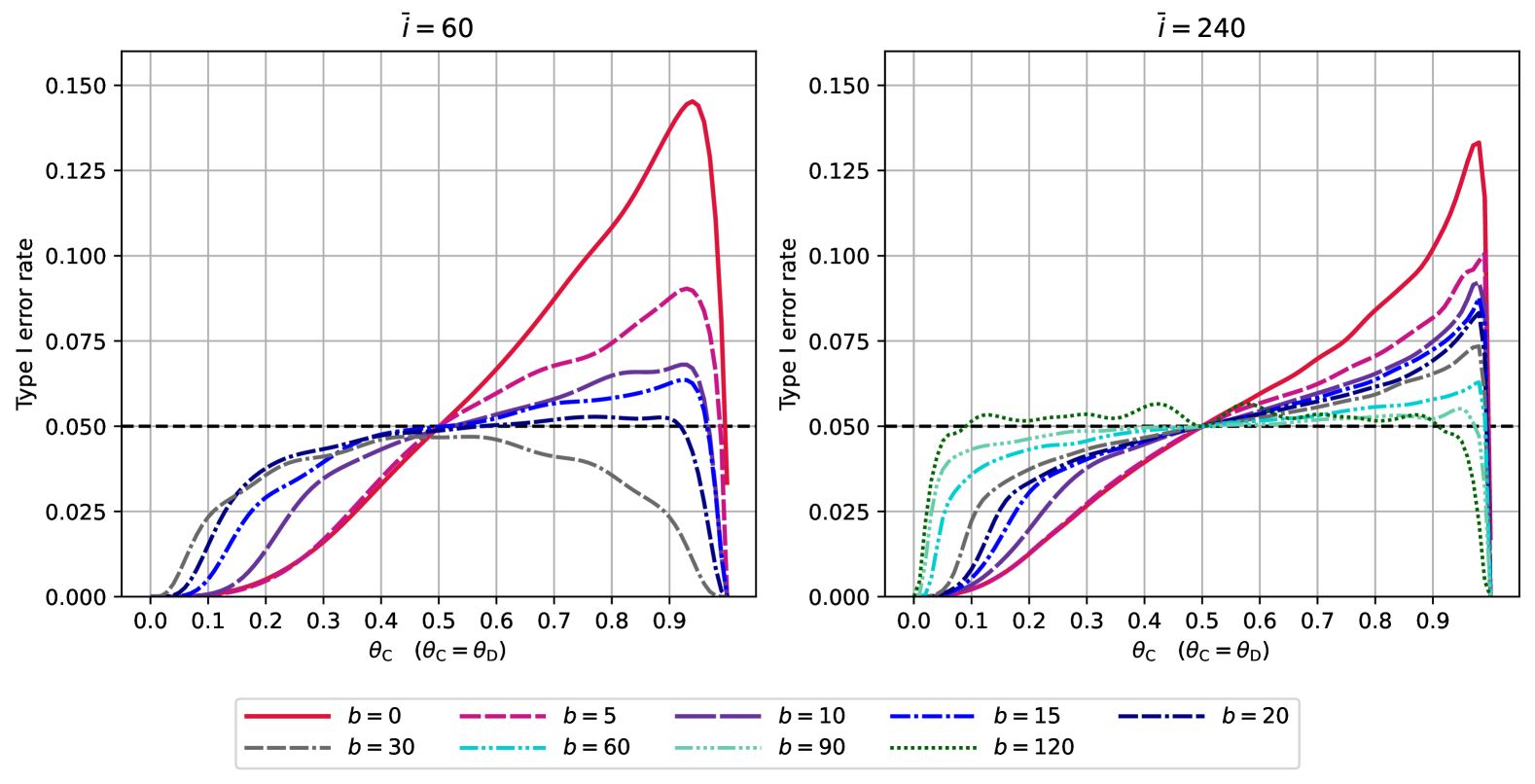
Figure 1: Type I error rate profiles for the Bayesian response-adaptive randomization design with calibrated test (calibrated for $\theta_{\text{C}}=\theta_{\text{D}}=0.5$) based on the posterior probability of control superiority for trial sizes $\bar{i}=60$ and $\bar{i}=240$, across $\theta_{\text{C}}=\theta_{\text{D}}\in\{0.00,0.01,\dots,1.00\}$ for different burn-in lengths $b$. The significance level $\alpha$ was set to $0.05$ (indicated by the horizontal dashed line).

To keep the type I error rate roughly under 6%, Figure 1 suggests the burn-in length to be more than a quarter of the trial size (i.e., $b>{\bar{i}}/4$). For ${\bar{i}}\geq 60$ we show that this indeed seems to be a valid rule of thumb in the case of a two-arm BRAR and when testing $H_{0}$ using the calibrated PPCS test. Table 1 shows the grid-approximated maximum type I error rate of the calibrated PPCS test versus $b$ for $\bar{i}\in\{20,40,60,80,100,240\}$. Table 1 shows that when the burn-in proportion (BP) is higher than or equal to $0.6$, the type I error rate is controlled at $6\%$ for ${\bar{i}}\geq 60$.

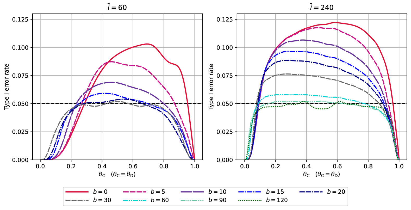
Figure 7: Type I error rate profiles for the Bayesian response-adaptive randomization design using the asymptotic Wald test for trial sizes $\bar{i}=60$ and $\bar{i}=240$, across $\theta_{\text{C}}=\theta_{\text{D}}\in\{0.00,0.01,\dots,1.00\}$ for different values of burn-in length $b$. The significance level $\alpha$ was set to $0.05$.

In conclusion, the use of calibrated tests leads to a substantial risk of type I error inflation under parameter misspecification, and this problem cannot be fully eliminated by increasing the burn-in length. Due to regulatory demands for strict type I error control, we study burn-in length’s effect on OCs with an exact test. In Appendix C Table 5 and Figure 7 the same evaluation is performed when instead of considering the PPCS as the test statistic, we use the Wald statistic with the Agresti-Caffo adjustment as defined in Baas et al. (2024, Equation (14)). We use a standard asymptotic two-sided Wald test (2.5% significance) instead of a calibrated test, common in theory but rare in BRAR trials with burn-in. (see, e.g., Table 2). are furthermore provided in Appendix C. The finite-sample and asymptotic properties of the Wald test under RA procedures are discussed in Baldi Antognini et al. (2022).

Table 1: Maximum type I error rate (in %) across the whole parameter space (using a grid approximation) of the calibrated test (calibrated for $\theta_{\text{C}}=\theta_{\text{D}}=0.5$) based on the posterior probability of control superiority (significance level $\alpha=0.05$) under the fully sequential BRAR design as the burn-in length varies. Burn-in proportion (BP) is the proportion of the trial within the burn-in stage, given by BP$=2b/\bar{i}$. BP$=1.0$ corresponds to equal allocation. Type I error rates above $6\%$ are indicated in bold (red).

BP	0	0.10	0.20	0.30	0.40	0.50	0.60	0.70	0.80	0.90	1.00
${\bar{i}}=$ 20	12.72	13.71	10.68	9.54	8.02	5.69	6.20	5.13	6.22	5.43	5.00
${\bar{i}}=$ 40	14.59	12.48	8.55	7.07	6.23	6.39	6.02	5.84	5.40	4.91	6.09
${\bar{i}}=$ 60	14.53	11.04	8.59	7.20	6.76	6.36	5.47	5.62	5.15	4.99	4.69
${\bar{i}}=$ 80	15.07	9.83	8.37	7.42	6.60	6.21	5.72	5.31	5.47	5.23	5.04
${\bar{i}}=$ 100	14.56	9.44	8.10	7.23	6.95	6.29	5.78	5.49	5.62	5.23	5.07
${\bar{i}}=$ 240	13.32	9.01	7.83	7.24	6.64	6.30	5.63	5.40	5.16	5.09	5.66

The main differences between the results for PPCS and the Wald statistic are that the type I error rate profile for the Wald test is more symmetrical, while the maximum type I error rate inflation for $b=0$ is slightly lower than for PPCS, around 10%-12% (Figure 7). Due to the more symmetrical type I error rate profile. The commonalities with the PPCS test are that the rule $b>{\bar{i}}/4$ works for controlling type I error rate at $6\%$ (in this case, even for all values of ${\bar{i}}$, see Table 5).

4.2 The added value of a burn-in when exact tests are applied in BRAR designs

This section presents the results for the exact tests given in Section 3.1 using the PPCS statistic under RA procedure $\pi^{\text{B}}_{b}$ for different burn-in lengths $b$. Note that for each burn-in length $b$ and type of exact test, a different critical value is derived. To give some intuition, we provide some of these critical values in Appendix B, where we also include critical values for the Wald test. We compare the CX-S test and UX test in terms of statistical power, as both of them control the type I error rate.

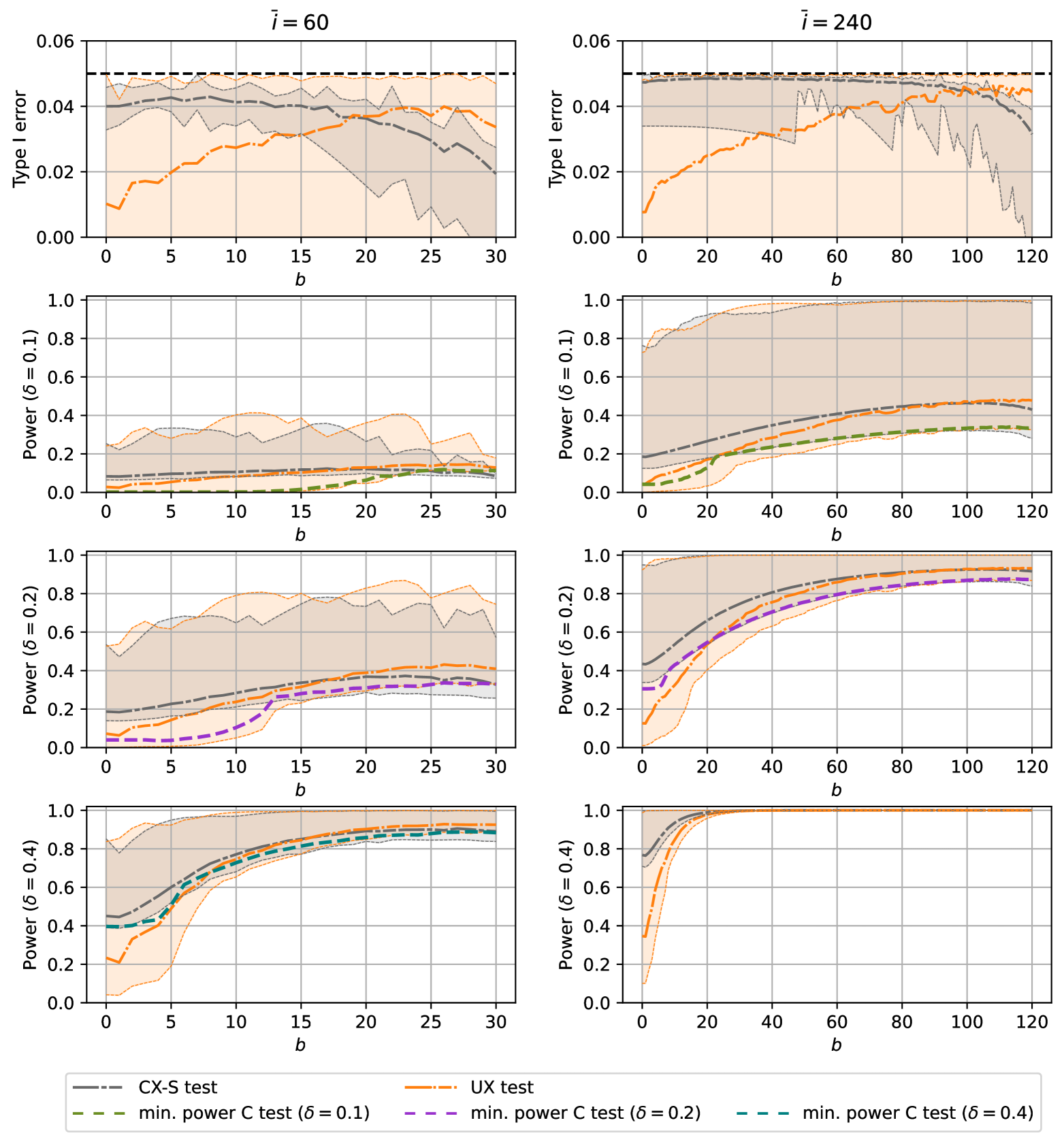
Figure 2: Type I error rate and power under treatment effects $\delta\in\{0.1,0.2,0.4\}$ for the Bayesian response-adaptive randomization design using the unconditional exact (UX) test and conditional exact test based on total successes (CX-S test) based on the posterior probability of control superiority with trial size ${\bar{i}}=60$ and ${\bar{i}}=240$ across different burn-in lengths. For comparison, we have plotted the (grid-approximated) minimum power for the calibrated (C) test for ${\bar{i}}=60$, $\delta\in\{0.1,0.2,0.4\}$ and ${\bar{i}}=240$, $\delta\in\{0.1,0.2\}$. The averages for each treatment effect $\delta$ and fixed burn-in length are represented by thick lines, while the minimum and maximum are presented by thin dotted lines and the ribbons. The significance level $\alpha$ was set to $0.05$.

The graphs in the first row of Figure 2 show the average, and grid-approximated minimum and maximum type I error rate across different burn-in lengths. As expected with exact tests, both the UX and CX-S tests maintain strict type I error control at 5% across all burn-in lengths, ensuring a maximum type I error rate of 5%. As $b$ increases, the average type I error rate for the UX test increases, while it decreases for the CX-S test. Hence, the UX (CX-S) test could be overly conservative when the burn-in length is small (large). The minimum and maximum type I error rate for the CX-S test shows a highly non-smooth behaviour, which follows from the fact that the critical values for these tests are different for each burn-in length, and by the discreteness of binary tests in general. Increasing $b$ exacerbates this behaviour, leading to a narrower range of treatment group sizes. Figure 2 shows that the type I error rate for the UX test varies between 0% and 5% for all burn-in lengths, yet the CX-S test shows much less variability over the parameter space and is less conservative than the UX test for smaller burn-in lengths, where the minimum type I error rate is around or higher than 3% for $b$ up to ${\bar{i}}/4$. On the contrary, the maximum type I error rate for the CX-S test decreases for larger values of $b$, where the maximum type I error rate for CX-S is smaller than the average type I error rate of the UX test in case $b={\bar{i}}/2$ for both ${\bar{i}}\in\{60,240\},$ indicating that the CX-S test might be overly conservative for larger burn-in lengths.

We note that for $b={\bar{i}}/2$, the CX-S test equals Fisher’s exact test (Fisher, 1934), while the UX test equals Barnard’s test (Barnard, 1945). Fisher’s exact test is known to be more conservative than Barnard’s test in the case of equal treatment group sizes and relatively small sample sizes (Mehrotra et al., 2003).

The three bottom rows in Figure 2 show how the minimum, maximum and average power to under treatment effects $\delta\in\{0.1,0.2,0.4\}$ vary across different burn-in lengths. The average power for $b={\bar{i}}/2$ is higher than for $b=0$ for both exact tests, however, the average power does not increase monotonically in the burn-in length. For the CX-S test, the average power can furthermore attain a maximum at $b<{\bar{i}}/2$, e.g., when ${\bar{i}}=240$ the maximum occurs around $b=100.$

Figure 2 shows that for ${\bar{i}}=60$ the average power for the CX-S test is higher than that of the UX test when $b<\bar{i}/4$, while it is lower for $b\geq\bar{i}/4$. We note that, generally, the power differences between the two tests are smaller in the latter situation ($b\geq\bar{i}/4$) than in the former situation ($b<\bar{i}/4$). For ${\bar{i}}=240$ and $\delta\in\{0.1,0.2\}$ the CX-S test has higher average and minimum power up to $b=80$. This agrees with Baas et al. (2024), showing CX-S test’ higher power over UX test for many RA procedures with a high degree of response-adaptiveness. A potential explanation of this phenomenon lies in the high dependency (for more aggressive RA procedures) of the distribution of treatment group sizes on total successes. On the contrary, for larger burn-in lengths this is not the case and the power of the CX-S test suffers from the higher discreteness of the conditional distribution of the test statistic. Figure 2 shows a large spread in the power for the UX test for, e.g, $\delta=0.2$ and ${\bar{i}}=60$ and $\delta=0.1$ and ${\bar{i}}=240$, as indicated by the maximum and minimum power values. This could be due to the highly asymmetrical type I error rate profile for the PPCS test, hence the UX PPCS test is overly conservative for certain parameter values. Lastly, Figure 2 shows that the minimum power for the CX-S test is higher than the minimum power for the calibrated test for at least a few burn-in lengths (indicated by dashed thick lines). This outperformance mainly happens for low success rates, where the calibration test was also shown to be conservative. Hence, the CX-S test has, for some parameter configurations, higher power than the commonly used calibration test with the added benefit of being exact.

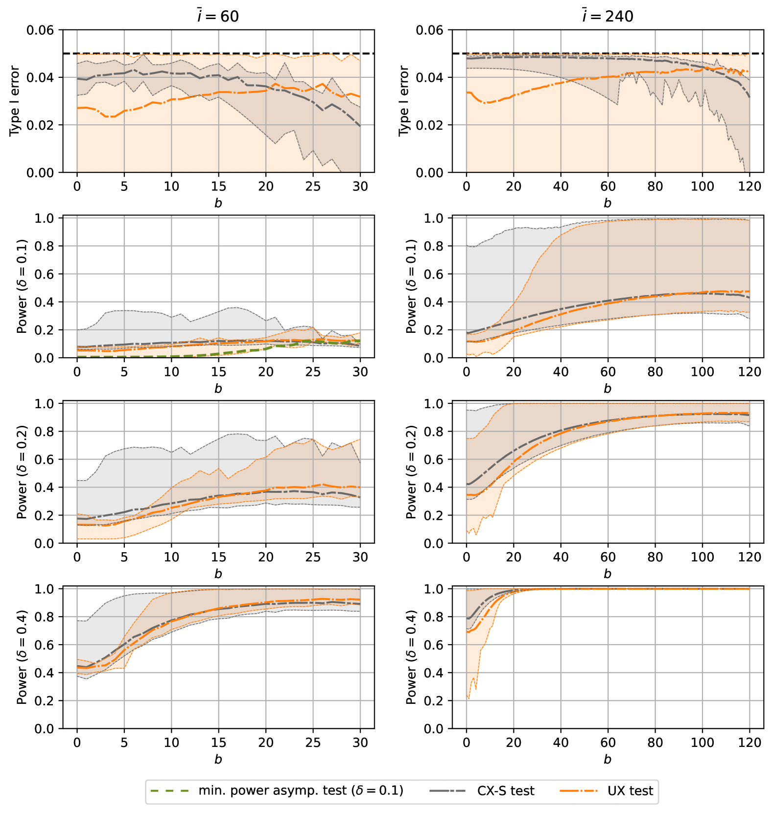
Figure 8: Type I error rate and power under detect treatment effects $\delta\in\{0.1,0.2,0.4\}$ for the Bayesian response-adaptive randomization design using the unconditional exact (UX) and conditional exact Wald test based on total successes (CX-S test) with trial size ${\bar{i}}=60$ and ${\bar{i}}=240$ across different burn-in lengths. For comparison we have plotted the (grid-approximated) minimum power for the asymptotic Wald test for ${\bar{i}}=60$ and $\delta=0.1$. The averages for each treatment effect $\delta$ and fixed burn-in length are represented by thick lines, while the minimum and maximum are presented by thin dotted lines and the ribbons. The significance level $\alpha$ was set to $0.05$.

In Appendix C Figure 8 the same evaluation is again performed for the Wald test instead of the PPCS test. The CX-S Wald test often shows higher maximum power than the UX Wald test, while less often showing lower minimum power than the asymptotic Wald test (only for $\delta=0.10,{\bar{i}}=60$) than under the calibration PPCS test comparison. The CX-S test again does better than the UX test when $b<\bar{i}/4$ and vice versa for $b\geq\bar{i}/4$, and maximum average power values are again found for $b<{\bar{i}}/2.$

Optimal burn-in proportion across the parameter space

Figure 3 shows the optimal burn-in proportion in terms of power (P-OBP) for the UX and CX-S test for each parameter configuration $\theta_{\text{C}},\theta_{\text{D}}\in\{0.00,0.01,\dots,1.00\}$. As the calibrated test does not control type I errors for every parameter configuration, this test was not considered in this evaluation. Note that the P-OBP can only be exactly computed using our calculation method, finding these maxima using simulation is prohibitive through Monte Carlo errors combined with the fluctuating and non-smooth behaviour of the power in the burn-in length.

The patterns in Figure 3 are hard to explain. Due to the discreteness of the binary tests, with changing critical values as the burn-in length changes, the power curve as a function of the burn-in length has a highly non-smooth behaviour and can suddenly jump to a high value. What first stands out in Figure 3 is that the P-OBP for power is often less than $1.00$ for ${\bar{i}}=60$. For the UX test it is often higher than 0.8, whereas for the CX-S test the P-OBP is often lower (especially around the diagonal). For ${\bar{i}}=240$ the P-OBPs are higher; the values for the UX test are closer to 1.0 than for ${\bar{i}}=60$ and the values for the CX-S test are again lower (especially around the diagonal).

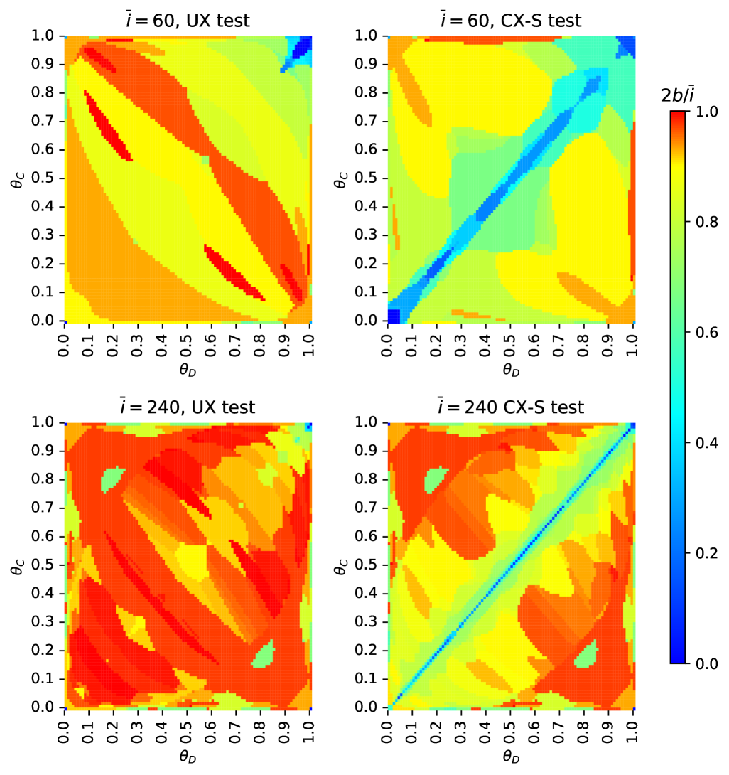
Figure 3: Optimal burn-in proportions ($2b/{\bar{i}}$) in terms of power of the Bayesian response-adaptive randomization design using the unconditional exact (UX) and conditional exact test based on total successes (CX-S test) based on the posterior probability of control superiority for every parameter configuration in the grid $\theta_{\text{C}},\theta_{\text{D}}\in\{0.00,0.01,\dots,1.00\}.$ The considered trial sizes are ${\bar{i}}=60$ and ${\bar{i}}=240$ participants.

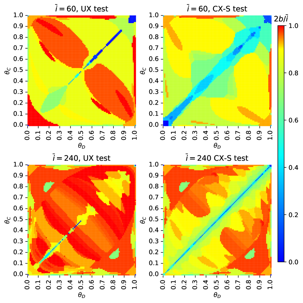
Figure 9: Optimal burn-in proportions ($2b/{\bar{i}}$) in terms of power of the Bayesian response-adaptive randomization design using the unconditional exact (UX) and conditional exact test based on total successes (CX-S test) based on the Wald test statistic for every parameter configuration in the grid $\theta_{\text{C}},\theta_{\text{D}}\in\{0.00,0.01,\dots,1.00\}.$ The considered trial sizes are ${\bar{i}}=60$ and ${\bar{i}}=240$ participants.

In conclusion, for the considered trial sizes the P-OBP for power depends heavily on the choice of test and is often not equal to one. Figure 9 in Appendix C contains the P-OBP plots when the Wald statistic is used instead of PPCS, where overall the findings are the same as for PPCS. The subfigures for the CX-S test are very similar to the ones in Figure 3 where, upon inspecting the results, numerical differences were seen although they were very small. This could be explained by the fact that the CX-S test fixes total successes, hence the behaviour of this test is less sensitive to the choice of the test statistic. Larger differences are indeed seen for the UX test, where for ${\bar{i}}=60$ higher P-OBPs are seen for the Wald test than for the PPCS test.

4.3 Impact of burn-in length on participant benefit metrics

One of the the main arguments in the literature for using RA procedures is the potential to allocate more participants to the better treatment. This section investigates the behaviour of EPASA and PIWD(0.1) as we vary the burn-in length. Note these metrics are not inference-related, hence test-independent.

EPASA and PIWD(0.1) for different burn-in lengths

The top row in Figure 4 shows the average and grid-approximated minimum and maximum EPASA versus the burn-in length for treatment effects $\delta\in\{0.1,0.2,0.4\}$. As expected, for every treatment effect $\delta$, lower burn-in lengths give a higher average, minimum and maximum EPASA, and increasing the sample size and increasing $\delta$ raises EPASA. A surprising observation here is that EPASA does not necessarily decrease as the burn-in length increases, e.g., the maximum average EPASA occurs for $b=1$ when $\bar{i}=60,\delta=0.1$. The average, minimum and maximum EPASA increases initially, then decreases slowly, and then it decreases linearly as $b$ increases. One explanation is that a longer burn-in will more likely identify the better arm, leading to almost all participants being allocated to the best arm in the response-adaptive phase, tracing out a straight line on the EPASA graph.

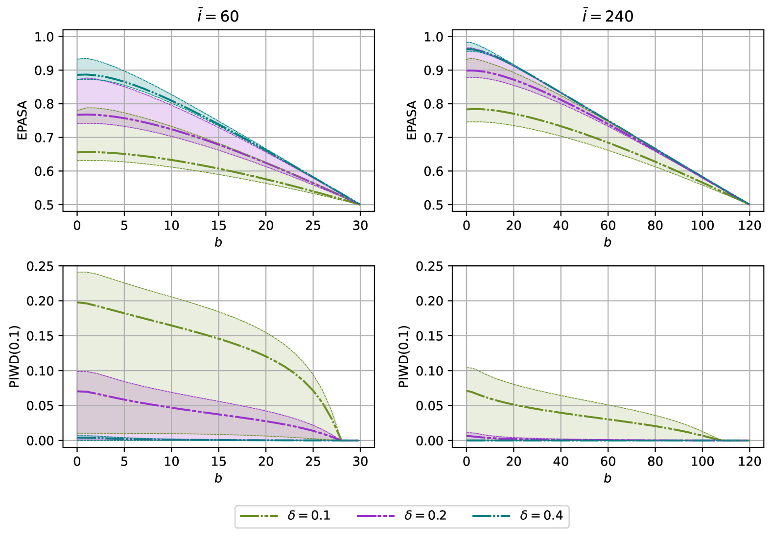
Figure 4: Expected proportion of allocations on the superior arm (EPASA) and probability of an imbalance in the wrong direction (PIWD(0.1)) under different burn-in lengths $b$ and treatment effects $\delta\in\{0.1,0.2,0.4\}$.The averages for each treatment effect $\delta$ and fixed burn-in length are represented by thick lines, while the minimum and maximum are presented by thin dotted lines and the ribbons.

The bottom row in Figure 4 shows that the average and grid-approximated minimum and maximum PIWD(0.1) decrease as we increase the burn-in length. The lines are in agreement with Robertson et al. (2023), who state that more aggressive RA procedures are more likely to have higher probabilities of imbalances in the wrong direction, which in our case would correspond to a lower burn-in length. As expected, for any fixed $\delta$, lower burn-in lengths give a higher PIWD(0.1), while increasing sample size and increasing $\delta$ reduces this OC. Initially for small burn-in lengths, PIWD(0.1) decreases in a roughly linear fashion, then towards the end, the PIWD(0.1) drops steeply towards 0. This is because for $b>{\bar{i}}(1-\varphi)/2$ it is impossible to achieve imbalance in the wrong direction.

For both metrics, the variation over the parameter space for $\delta=0.1$ is larger than variation for $\delta\in\{0.2,0.4\}$. It is difficult for the RA procedure to detect a small treatment effect. That said, for $\delta\geq 0.2$ and $\bar{i}=240$ the PIWD(0.1) is less than $1\%$ regardless of the burn-in length, so we almost certainly improve in-trial participant benefit when the treatment effect is not too small given the trial size.

While it may seem alarming that the average PIWD(0.1) for $\bar{i}=60,\delta=0.1$ can get as high as 20% for small burn-in lengths, we highlight that the interpretation of the PIWD metric is not straightforward. The fact that PIWD(0.1)$=0.2$ for a treatment effect difference $\delta=0.1$ indicates that we have a 20% probability of having 10% less expected successes for at least 55% of trial participants (i.e. an imbalance of allocations to the worse arm of at least 10%). The severity of this imbalance still depends on the probability of having an even worse misallocation, such as 65% of participants being allocated to the worst arm. If this is zero, then the situation would not be severe after all, since for fixed equal allocation and $\delta=0.1$ the probability of having 10% less expected successes for 50% of participants is 100%. Hence, although we are only considering one imbalance measure, we recommend looking at different imbalance measures when choosing a burn-in length (e.g., PIWD$(\varphi)$ for different values $\varphi$).

PIWD(0.1) across the parameter space

Figure 5 presents a heatmap of values of PIWD(0.1) across the parameter space, where we restrict to a grid of values $\theta_{\text{C}},\theta_{\text{D}}\in\{0.01,0.02,\dots,1.00\}$ with $\theta_{\text{C}}\neq\theta_{\text{D}}$ which gives a clearer picture on where the imbalance occurs.

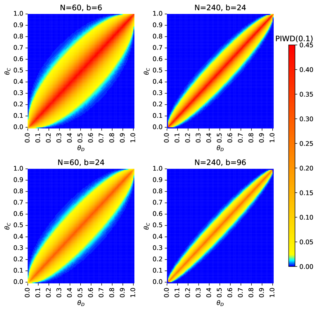
Figure 5: Probability of an imbalance in the wrong direction (PIWD) across the parameter space for $\theta_{\text{C}},\theta_{\text{D}}\in\{0.00,0.01,\dots,1.00\}$. burn-in lengths $b\in\{0.1\bar{i},0.4\bar{i}\}$ are considered, as well as trial sizes ${\bar{i}}\in\{60,240\}$.

As also indicated in Robertson et al. (2023) (who restricted to the case $\theta_{\text{C}}=0.25$, $\theta_{\text{D}}\geq\theta_{\text{C}}$ and ${\bar{i}}=200$), Figure 5 shows that the PIWD(0.1) is highest near the diagonal $\theta_{\text{C}}=\theta_{\text{D}}$. The graphs on the bottom row correspond to higher burn-in lengths and show a smaller PIWD(0.1) compared to the top row. Hence, the maximum of PIWD(0.1) shown in Figure 4 happens around the point $(1/2-\delta/2,1/2+\delta/2)$. One of the limitations of the PIWD(0.1) metric is that it is large when the difference in treatments is smallest, and so the cost of allocating to the wrong treatment is lowest, as noted in Robertson et al. (2023). Inspection of the numerical results shows that the heatmaps are not symmetrical around the line $\theta_{\text{C}}+\theta_{\text{D}}=1$, which is not noticeable from visual inspection. An explanation could be that the arm with the highest variance switches when comparing a parameter vector with its reflection along the line $\theta_{\text{C}}+\theta_{\text{D}}=1$, hence for one of these scenarios it is more difficult to identify the best arm. For example, comparing the vector $(0.4,0.5)$ with $(0.5,0.6)$ the superior arm has the highest variance for the first parameter vector, while for the second it has the smallest variance.

4.4 Recommendation for burn-in

The general takeaway from our analysis is that, while providing a more balanced type I error rate profile for common tests such as calibration and asymptotic tests, the choice of the burn-in period cannot be used to control the type I error rate completely over the parameter space for such tests when applying $\pi_{b}^{\text{B}}$. Non-exact tests, when applied with insufficient burn-in lengths, can exhibit substantial type I error inflation, approaching three times the nominal significance level. Therefore, practitioners should exercise caution when using calibrated or asymptotic tests, unless their statistical properties have been thoroughly investigated through simulation or exact methods, as demonstrated in this paper. As our numerical results show, a good rule of thumb if type I error control is not the highest priority (e.g., in exploratory settings), could be to set $b={\bar{i}}/4$ for the BRAR design with a burn-in. this choice of burn-in length might lead to acceptable operating characteristics for calibrated or asymptotic tests, as, in our results, it led to a balanced type I error rate profile, where the average type I error rate is below the significance level, while the power plateaus for higher burn-in lengths.

In settings where strict type I error control is required (e.g., in confirmatory settings), we recommend considering exact tests. In such settings, type I error rate control is a given and the burn-in length can be set such that a sufficient power is reached. As we saw that for burn-in lengths at least up to ${\bar{i}}/4$ the CX-S test has higher average power than the UX test, the CX-S test could be preferred in designs that at least target a moderate amount of response-adaptivity. The above guidelines do not consider the PIWD(0.1) due to the difficulties with the interpretation of this OC (as indicated in Section 4.3). We note that if type I error and power are not deemed important at all, it might still be better to use a burn-in, as the maximum average EPASA for our considered trial sizes occurs at small but positive values of the burn-in length.

The guidelines above mainly focus on the average OCs. Since different trials have different priorities, practitioners may also set threshold values for the OCs which suit their needs, and then investigate which burn-in length satisfies the conditions. As we saw that the power and EPASA can have a non-monotonic behaviour in the burn-in length, it is recommended to inspect more burn-in lengths than just $b=0$ and $b={\bar{i}}/2$, and inspect at least the values of $b$ close to these two endpoints. This recommendation is further supported by the optimal burn-in proportions presented in Figures 3 and 9, where many burn-in lengths are found that maximize power which are strictly between 0 and ${\bar{i}}/2.$

Let us now give an example in a more specific setting. Suppose we want to run a trial with $\bar{i}=240$ participants, hoping to achieve a minimum power of 80%  under a treatment effect $\delta=0.2$ at a 5% significance level, while keeping PIWD(0.1) $<5\%$ in $\Theta_{0.2}$. If strict type I error control is required, then we can use exact tests. Figure 2 shows that minimum power can be attained using the CX-S test with $b=63$ or UX test with $b=68$. If we are lenient with type I error control, we can use the calibration test with maximum type I error rate $<6\%$. A numerical evaluation then shows that $b=63$ would be sufficient. For $\delta=0.2,$ PIWD(0.1) is very close to zero for $b\geq 60$, which does not put further restrictions on $b$. Thus we can recommend $b=63$ for the calibrated test, $b=63$ for the CX-S, and $b=68$ for the UX test as it maximizes the EPASA while fulfilling all the threshold values for the OCs. We would prefer to use the CX-S test in this scenario, which yields the same participant benefit, while it has a stronger control on the type I error than the calibration test. From this example, we see that even when type I error control is not of highest importance, an exact test might give more desirable OCs.

5 Real-world application: ARREST trial

In this section, we consider the effect of the burn-in length on the operating characteristics of the Advanced R²Eperfusion STrategies for Refractory Cardiac Arrest (ARREST) trial described in Yannopoulos et al. (2020), where we also consider the use of an unconditional exact test. The CX-S OST is omitted here, as the combination of this test with early stopping is not straightforward. We analyze the effect of different burn-in lengths on the unconditional OCs following from the trial design, i.e., we do not condition on the realised size of the trial.

In the ARREST trial, extracorporeal membrane oxygenation (ECMO) facilitated resuscitation (developmental) was compared to standard advanced cardiac life support (control) in adults with an out-of-hospital cardiac arrest and refractory ventricular fibrillation. The inferential goal of the trial was to test $\theta_{\text{D}}=\theta_{\text{C}}$ versus $\theta_{\text{D}}\geq\theta_{\text{C}}$, where a success ($Y_{a,i}=1$) represented survival to hospital discharge.

Participants were allocated treatment in groups of 30 under a permuted block design, with a control group allocation probability equal to the posterior probability (based on independent uniform priors) that the control treatment is superior, restricted between 0.25 and 0.75 (i.e., the clip method as defined in Du et al. (2018)). If at any of the interim analyses either the PPCS or one minus the PPCS became higher than an optional stopping threshold (OST) of $0.986$, the recommendation was made to stop the trial early for futility or superiority, respectively. This OST was calibrated based on a success rate of $0.12$ under the null hypothesis, and controlled type I error rate at 0.05 based on a simulation study of 10,000 samples. The considered alternative hypothesis $\theta_{\text{C}}=0.12$ and $\theta_{\text{D}}=0.37$ (based on a treatment effect of $0.25$) yielded a power around $90\%$. The ARREST trial stopped for efficacy of the ECMO treatment after allocating the first group of 30 participants, with posterior probability of superiority of 0.9861.

In Baas et al. (2024) this trial was re-analyzed, where the calibrated (C) OST was compared to an UX OST. The UX OST was computed based on an extension of the Markov chain $(\bm{X}_{t})_{t}$ defined in Section 2, where the extension of $(\bm{X}_{t})_{t}$ also models the optional stopping component of the trial. It was shown that while the UX OST bounds type I error rate by $0.05$ over the whole of the parameter space, it also leads to a decrease in power and EPASA. Due to the optional stopping component EPASA, assuming $\theta_{\text{D}}\geq\theta_{\text{C}}$, is defined as:

$$\mathbb{E}_{\text{\boldmath$\mathbf{\theta}$}}^{\pi}[(N_{\text{D},i_{U}}+({\bar{i}}-i_{U})\mathbb{I}(\text{Optional stopping in favour of~$\text{D}$}))/{\bar{i}}]$$

where $U$ is the interim analysis at which the trial stops, the EPASA hence considers the fraction of participants allocated to the developmental treatment before and after optional stopping. It is hypothesised that a larger burn-in length will mitigate the large differences seen in EPASA and power across OSTs.

The ARREST trial had a maximum trial size of 150 participants and considered blocked allocation with blocks of $30$ participants, hence we can only have $b=15,30,45,60,75$ (noting that in the original design, the allocation probability could only be changed after $15$ participants were allocated per arm). During the burn-in period, the target allocation proportion is equal to $0.5$ (as before) and early stopping is only possible after allocating participant $i\geq 2b.$ The Markov chains for computing the UX OST and the OCs described in Baas et al. (2024) were adapted to account for a longer burn-in length by decreasing the number of interim analyses and setting the first interim analysis at $i=2b$. The original C OST $0.986$ was used for $b=15$, while for $b>15$ the C OST was determined using the procedure outlined in Baas et al. (2024, Section 5) where the only value under the null hypothesis considered was $\theta_{\text{C}}=\theta_{\text{D}}=0.12$. The same procedure (taking all possible success rates into account) was used to determine the UX OST.

Figure 6 shows a star plot of the EPASA, power, minimum true negative rate (MTNR, minimum value of one minus the type I error rate) and probability of no imbalance in the wrong direction (PNIWD(0.1)). For all OCs, a higher value is better. The EPASA, power, and PNIWD(0.1) were calculated under the alternative $\theta_{\text{C}}=0.12,$ $\theta_{\text{D}}=0.37$, while the MTNR was calculated over the range $\theta_{\text{C}}=\theta_{\text{D}}\in\{0.020,0.03,\dots,0.22\}$.

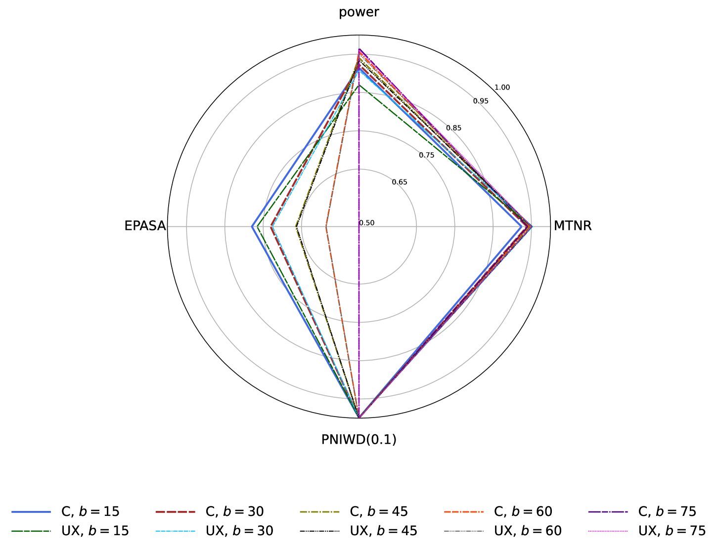
Figure 6: Star plot comparing the expected proportion of allocations on the superior arm (EPASA), power, minimum true negative rate over interval $\theta_{\text{C}}=\theta_{\text{D}}\in\{0.02,0.03,\dots,0.22\}$ (MTNR), and probability of no imbalance in the wrong direction (PNIWD(0.1)) for the ARREST trial when using a calibrated (C) and unconditional exact (UX) optional stopping threshold combined with a burn-in $b$ of $15,30,45,60,$ and $75$ participants per arm.

Figure 6 shows that the EPASA decreases in $b$, while the power increases. The EPASA for the C OST designs is higher than for the UX OST designs due to the higher power under the C OSTs, which means that the trial stops earlier for superiority under the alternative. For $b<75,$ the type I error rate is not controlled under the C OST for $\theta_{\text{C}}=\theta_{\text{D}}\in\{0.02,0.03,\dots,0.22\}$, corresponding to an MTNR less than $0.95$, whereas for the other designs, the type I error rate is under control. Figure 6 shows that the PNIWD(0.1) is very similar across different designs, it ranges from $0.999$ to $1.00$, in agreement with Figure 5 which shows that PIWD(0.1) is largest when treatment effects are small. As hypothesized, the differences in the OCs between the C OST and UX OST, mainly EPASA and power, decrease in $b$.

The star plot can be used to propose designs based on trade-offs in the OCs and to make a choice of clinical design, including burn-in length, based on multiple trial objectives. If type I error rate control at level $0.05$ is not of the highest importance, Figure 6 shows that a good option could be to use the C OST with $b=15.$ If the type I error rate should be controlled, one design which stands out is the UX OST design with $b=30$, showing a lower EPASA but similar power to the previously mentioned design. If EPASA is of higher importance than power, then the UX OST design with $b=15$ might be best. If EPASA is not important at all, the C OST design with $b=75$ would be the best option, yielding a power higher than $95\%$.

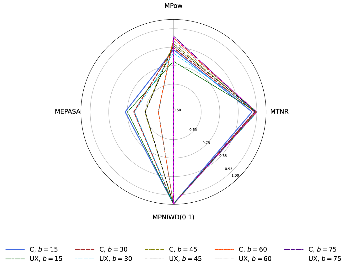
Figure 10: Star plot comparing the minimum expected proportion of allocations on the superior arm (MEPASA), minimum power (MPow), minimum true negative rate over interval $\theta_{\text{C}}=\theta_{\text{D}}\in\{0.02,0.03,\dots,0.22\}$ (MTNR), and minimum probability of no imbalance in the wrong direction (MPNIWD(0.1)) for the ARREST trial when using a calibrated (C) and unconditional exact (UX) optional stopping threshold combined with a burn-in $b$ of $15,30,45,60,$ and $75$ participants per arm. The minimum is taken over $\theta_{\text{C}}=\theta_{\text{D}}-\delta\in\{0.02,0.03,\dots,0.22\}$ where $\delta=0$ for the null hypothesis and $\delta=0.25$ for the alternative hypothesis.

Figure 10 shows the same evaluation for a range of alternative hypotheses $\theta_{\text{C}}=\theta_{\text{D}}-0.25\in\{0.02,0.03,\dots,0.22\}$. The behaviour of the minimum PNIWD(0.1) (MPNIWD(0.1)) in Figure 10 is similar to the PNIWD(0.1) in Figure 6. The power seems to be the most sensitive to the scenario considered, as the minimum power (MPow) is substantially lower than in Figure 6. The MPow for the UX test with $b=15$ is less than the (usually chosen threshold of) $0.8$, which might be a reason not to opt for this design despite it leading to exact type I error control and high (minimum) EPASA.

6 Discussion and recommendations

This paper considers the effect of an initial burn-in phase on the operating characteristics (OCs) of the Bayesian response-adaptive randomization (BRAR), i.e., Thompson sampling-based, design, where testing is performed either using a calibrated, conditional, or unconditional exact test. The analyses were based on the minimum, average, and maximum values of the OCs over the parameter space. In agreement with the literature, the burn-in length can be used to trade-off participant benefit and power, and to lower the probability of a treatment group size imbalance in the wrong direction.

Our numerical evaluation revealed several key insights. Firstly, calibrated or asymptotic tests exhibited significant type I error rate inflation compared to fixed designs with equal allocation, particularly in BRAR designs. While increasing burn-in length offered partial mitigation, it did not eliminate the inflation entirely. Secondly, exact tests demonstrated superior power over calibration or asymptotic tests in certain parameter settings, notably with a trial size of 60 participants and varying burn-in lengths. Furthermore, the conditional exact test displayed a consistent performance profile across the parameter space and was less conservative than calibrated and asymptotic tests, even with extended burn-in periods. Lastly, the choice of test statistic significantly impacted statistical operating characteristics; the Wald test, for instance, yielded a more balanced type I error rate profile and greater power than tests based on the posterior probability of control superiority.

Some general guidelines for choosing the burn-in length follow from our analysis. If type I error control is not of the highest priority, then a good rule of thumb might be to choose the burn-in length per arm roughly equal to the trial size divided by four for the BRAR design. This burn-in length led to a more balanced type I error rate profile, while power was similar for higher burn-in lengths. In settings where type I error control is strictly required (e.g., in confirmatory settings), we recommend considering exact tests. In this case, the burn-in length could be chosen such that a sufficient power value is reached, possibly at a lower value than the trial size over four. The conditional exact test would be preferred, as our numerical evaluation showed that this test has higher power than the unconditional exact test in terms of average (and often minimum) power for small to moderate burn-in lengths.

The optimal burn-in length in terms of power or participant benefit is often different from the minimum or maximum possible value, hence our recommendation is to inspect more burn-in lengths than just the minimum (i.e., zero) and the maximum (i.e., trial size over two) and inspect at least the values of $b$ close to these two endpoints, in contrast to the guidelines given in Du et al. (2018). The above guidelines focus on the behaviour of the average OCs, whereas in specific settings expert opinion might better guide the burn-in length, e.g., through a desired minimum power or maximum allowed type I error rate.

The penultimate section of this paper considers an illustrative application to a real-world Bayesian adaptive clinical trial with optional stopping. The trial had a complex nature, where allocation was performed in blocks based on a permuted block design and the trial stopped when, at interim, the posterior probability of superiority crossed a calibrated optional stopping threshold. Based on the Markov chain modelling framework in Baas et al. (2024), we evaluated the performance of the calibrated and unconditional optional stopping thresholds under different burn-in lengths. As it was assumed that after early stopping, the remaining participants were allocated the treatment that was deemed superior, the participant benefit depends on the optional stopping threshold of choice. The most sensitive OCs were participant benefit and power, and it was concluded that low burn-in lengths yielded a balanced trade-off.

In this paper, we considered the imbalance measure considered in Thall et al. (2015). This measure equals the probability of a substantial difference in the allocation proportion in the direction of the inferior arm. In agreement with Robertson et al. (2023), our results show that this probability increases as the treatment effect decreases in absolute value, but the impact of an imbalance in the wrong direction also diminishes in this case. Furthermore, the interpretation of this metric is not straightforward. The dichotomization in a right and wrong direction, without considering the actual effect on expected outcomes, is mentioned as a downside of this OC in Robertson et al. (2023). Future research could consider different imbalance measures or different values of the imbalance parameter.

Some interesting areas are left for future research, such as the combination with the clipping of allocation probabilities, power transformation (Du et al., 2018), the use of different prior configurations, an adaptive burn-in length instead of a fixed deterministic burn-in length, and the consideration of other clinical trial designs, e.g., multi-arm or multi-outcome designs or different outcome types. The effect of a time trend is furthermore also left for future work. Future research should establish practical guidelines for general response-adaptive designs, encompassing a wider range of operating characteristics. Developing theoretical results to elucidate the impact of burn-in length on various operating characteristics would offer deeper insight into its effects. While this study focuses specifically on BRAR designs which test using the posterior probability, our method can be readily used to analyze the effect of the burn-in length in other response-adaptive designs, e.g., those that target optimal proportions where Pin et al. (2025b) observed large type I error rate inflation. A comparative analysis of various calculation methods for posterior probability of superiority would provide valuable and complementary insights to this research.

Appendix A Selection and description of BRAR trials with a burn-in period

Table 2: Characteristics of multiple response-adaptive clinical trials using a burn-in period. Reference (Ref.) number refers to the number in the bibliography list given below.

Trial name/number(s)	Ref. number	Phase	Arms	Planned burn-in period	Target trial size	Early stopping	Justification of burn-in period	Randomization rule	Test(s) for primary endpoint
BATTLE / NCT00409968, NCT00411671, NCT00411632, NCT00410059, NCT00410189	1	2	4	80	250	N	Lowest possible to ensure $\geq 1$ patient in each marker group to complete treatment before starting RAR	BRAR with covariate adjustment	PPCS
BATTLE-2 / NCT01248247	2	2	4	70	200	N	Not specified	BRAR with covariate adjustment	None
ARREST / NCT03880565	3	2	2	30	$\leq$150	Y	Not specified	BRAR with clipping	PPCS (early stopping threshold 0.986)
ABT-089 / NCT00555204	4	2	7	$\geq$5 per arm	$\leq$400	Y	Not specified	BRAR	Posterior probability distributions/credible intervals
ADORE / NCT00807911	5	3	2	300	$\leq$1100	Y	Not specified	BRAR with variance adjustment	PPCS (early stopping threshold 0.99)
ESETT / NCT01960075	6	3	3	300	$\leq$795	Y	Not specified	BRAR	Posterior probability (interim, early stopping threshold 0.975), Chi-squared test (final)
PAIN-CONTRoLS/ NCT02260388	7	4	4	$\geq$20 per arm	$\leq$400	Y	Not specified	BRAR	Posterior probability (early stopping threshold 0.975)

Bibliography (RA clinical trial list)

1. Kim, E.S., Herbst, R. S., Wistuba, I. I., Lee, J. J., Blumenschein, G. R., Tsao, A., Stewart, D. J., Hicks, M. E., Erasmus Jr., J., Gupta, S., Alden, C. M., Liu, S., Tang, X., Khuri, F. R., Tran, H. T., Johnson, B. E., Heymach, J. V., Mao, L., Fossella, F., Kies, M. S., Papadimitrakopoulou, V., Davis, S. E., Lippman, S. M., Hong, W. K. (2011). The BATTLE trial: Personalizing therapy for lung cancer. Cancer Discovery 1(1), 44–53. https://doi.org/10.1158/2159-8274.CD-10-0010

2. Papadimitrakopoulou, V., Lee, J. J., Wistuba, I. I., Tsao, A. S., Fossella, F. V., Kalhor, N., Gupta, S., Byers, L. A., Izzo, J. G., Tang, X., Skoulidis, F., Gibbons, D. L., Shen, L., Wei, C., Diao, L., Peng, S. A., Wang, J., Tam, A. L., Heymach, J. V., Hong, W. K., Gettinger, S. N., Goldberg, S. B., Koo, J. S., Herbst, R. S., Miller, V. A., Coombes, K. R., Mauro, D. J., & Rubin, E. H. (2016). The BATTLE-2 study: A biomarker-integrated targeted therapy study in previously treated patients with advanced non-small-cell lung cancer. Journal of Clinical Oncology, 34(30), 3638–3647. https://doi.org/10.1200/JCO.2015.66.0084

3. D. Yannopoulos, J. Bartos, G. Raveendran, E. Walser, J. Connett, T. A. Murray, G. Collins, L. Zhang, R. Kalra, M. Kosmopoulos, R. John, A. Shaffer, R. J. Frascone, K. Wesley, M. Conterato, M. Biros, J. Tolar, and T. P. Aufderheide. Advanced reperfusion strategies for patients with out-of-hospital cardiac arrest and refractory ventricular fibrillation (ARREST): A phase 2, single centre, open-label, randomised controlled trial. The Lancet, 396(10265):1807–1816, 2020. https://doi.org/10.1016/S0140-6736(20)32338-2.

4. Lenz, R. A., Pritchett, Y. L., Berry, S. M., Llano, D. A., Han, S., Berry, D. A., Sadowsky, C. H., Abi-Saab, W. M., & Saltarelli, M. D. (2015). Adaptive, dose-finding phase 2 trial evaluating the safety and efficacy of ABT-089 in mild to moderate Alzheimer disease. Alzheimer Disease & Associated Disorders, 29(3), 192–199. https://doi.org/10.1097/WAD.0000000000000093

5. Carlson, S. E., Gajewski, B. J., Valentine, C. J., Kerling, E. H., Weiner, C. P., Cackovic, M., Buhimschi, C. S., Rogers, L. K., Sands, S. A., Brown, A. R., Mudaranthakam, D. P., Crawford, S. A., & DeFranco, E. A. (2021). Higher dose docosahexaenoic acid supplementation during pregnancy and early preterm birth: A randomised, double-blind, adaptive-design superiority trial. EClinicalMedicine, 36, 100905. https://doi.org/10.1016/j.eclinm.2021.100905

6. Chamberlain, J. M., Kapur, J., Shinnar, S., Elm, J., Holsti, M., Babcock, L., Rogers, A., Barsan, W., Cloyd, J., Lowenstein, D., Bleck, T. P., Conwit, R., Meinzer, C., Cock, H., Fountain, N. B., Underwood, E., Connor, J. T., Silbergleit, R., Neurological Emergencies Treatment Trials, & Pediatric Emergency Care Applied Research Network investigators. (2020). Efficacy of levetiracetam, fosphenytoin, and valproate for established status epilepticus by age group (ESETT): A double-blind, responsive-adaptive, randomised controlled trial. The Lancet, 395(10231), 1217–1224. https://doi.org/10.1016/S0140-6736(20)30611-5

7. Barohn, R. J., Gajewski, B., Pasnoor, M., Brown, A., Herbelin, L. L., Kimminau, K. S., Mudaranthakam, D. P., Jawdat, O., Dimachkie, M. M., & the PAIN-CONTRoLS Study Team. (2020). Patient Assisted Intervention for Neuropathy: Comparison of Treatment in Real Life Situations (PAIN-CONTRoLS): Bayesian adaptive comparative effectiveness randomized trial. JAMA Neurology, 77(5), 557–567. https://doi.org/10.1001/jamaneurol.2020.2590

Appendix B Tables with critical values

Table 3: Upper critical values per burn-in length $b$ for trial size ${\bar{i}}=60$ for the calibration test based on the posterior probability of control superiority (PPCS), the unconditional exact (UX) test based on PPCS, conditional exact PPCS test based on total successes (CX-S PPCS test) for 12 and 48 total successes, as well as the upper critical values when using the Wald test statistic for these tests instead of the PPCS. The right significance level was set to $2.5\%$. Trailing zeros are not displayed.

b	Calibration (PPCS)	UX PPCS	CX-S PPCS (S=12)	CX-S PPCS (S=48)	UX Wald	CX-S Wald (S=12)	CX-S Wald (S=48)
0	0.978233355395697	0.9947496072990138	0.9485264395008914	0.9927984157010034	2.302718174896149	3.9735970711951314	16.685322891691367
1	0.9781225779090684	0.9953212845230767	0.9485264395008914	0.9927984157010034	2.302718174896149	3.9735970711951314	16.685322891691367
2	0.978424114225277	0.992067689053411	0.9485264395008914	0.9927984157010034	2.314198293489495	3.9735970711951314	2.643304042534928
3	0.9790260525484195	0.9916672873845506	0.9485264395008914	0.9861681852935872	2.3348799378810092	3.9735970711951314	1.969777651208623
4	0.9805847153830307	0.9916672873845501	0.9485264395008914	0.9861681852935872	2.3069908920018367	3.9735970711951314	2.0000000000000004
5	0.9805847153830307	0.9898612626802341	0.9524953443194414	0.9861681852935872	2.244193077610112	3.9735970711951314	1.9560942740767506
6	0.979483984434495	0.9884376484509019	0.957389825103261	0.9850237556333951	2.217970823170696	3.9735970711951314	1.9103280233981044
7	0.9790260525484195	0.9881797899504889	0.957389825103261	0.9850237556333951	2.1920662875450887	3.986942522942203	1.894212202238607
8	0.9786845650880073	0.9861019884949906	0.957389825103261	0.9850237556333951	2.1496104640952374	3.986942522942203	1.894212202238607
9	0.9786845650880073	0.9849109348028043	0.957389825103261	0.9794839844346975	2.146561442983005	3.986942522942203	1.9420166249104487
10	0.9784545138738479	0.9848017659048213	0.9608623622030332	0.9848973252369821	2.1145598486192863	3.986942522942203	2.0000000000000004
11	0.9781640004387606	0.9839067305268394	0.969962204991043	0.9794839844346975	2.0961796002305153	4.014260294784796	1.9103280233981044
12	0.9776156670306634	0.9839067305268394	0.969962204991043	0.9794839844346975	2.083022575693182	4.014260294784796	1.830016782527511
13	0.9764862727469846	0.9820200951877319	0.9768885222819681	0.9779145861440016	2.0660294406384994	4.029304421069107	1.9103280233981044
14	0.9764862727469846	0.9820200951877319	0.9663733717955911	0.9848973252369821	2.06568306450296	2.388037076469809	1.969777651208623
15	0.9763391532922311	0.9818031890578925	0.9608623622030332	0.9779145861440016	2.021702176265099	2.388037076469809	1.9103280233981044
16	0.9759825519641755	0.9800594713363734	0.9608623622030332	0.9775738544502989	2.021702176265099	2.388037076469809	1.830016782527511
17	0.9757243012088005	0.9797834542199031	0.9608623622030332	0.9779145861440016	2.0217021762650984	2.388037076469809	1.9103280233981044
18	0.9756621681019739	0.9792993282725425	0.9707139671387696	0.9847392002468287	2.011594300028457	2.5131234497501733	2.0283702113484394
19	0.9759825519641755	0.9775738544503001	0.9707139671387696	0.9779145861440016	2.011594300028457	2.5131234497501733	1.9103280233981044
20	0.9761502054406046	0.9775738544503001	0.9784545138739889	0.9779145861440016	2.011594300028457	2.635081948268323	1.9103280233981044
21	0.9749982908819077	0.9774557869401455	0.9726534336515967	0.9683933684856809	1.9639359620800905	2.227784021228921	1.7747405374280212
22	0.9749982908819077	0.975475696405277	0.9663733717955911	0.9830678759741764	1.9924984760531164	2.1064127776663257	2.078036923180232
23	0.9749982908819077	0.975235086733878	0.9663733717955911	0.9830678759741764	1.9924984760531164	2.1064127776663257	2.078036923180232
24	0.9761854762466753	0.9766456353512373	0.9663733717955911	0.9830678759741764	2.0013843300632175	2.1064127776663257	2.078036923180232
25	0.9742791605266793	0.9754760637149245	0.9726534336515967	0.9734846398942882	1.9638370552058695	2.227784021228921	1.9420166249104487
26	0.9736205692491952	0.97401977359379	0.9803217074512501	0.9631244804017428	1.9493917067918949	2.3397979352670997	1.79867847541553
27	0.9761854762466762	0.9761854762466762	0.9852683841251674	0.9515529995231619	1.9936203984193257	2.4249119918964435	1.6753366866562536
28	0.976429464794035	0.9769204877646053	0.9628077487730287	0.9845660747738446	2.010841003245581	1.8841275935760935	2.2472576881857393
29	0.9785993142093347	0.9785993142093347	0.9628077487730287	0.9790555184650054	2.0455920583489493	1.8841275935760935	2.1467914292930836
30	0.9793538324121724	0.9793538324121724	0.9723027995475091	0.9723027995475023	2.06568306450296	2.0219862629219842	2.0219862629219842

Table 4: Upper critical values per burn-in length $b$ for trial size ${\bar{i}}=240$ for the calibration test based on the posterior probability of control superiority (PPCS), the unconditional exact (UX) test based on PPCS, conditional exact PPCS test based on total successes (CX-S PPCS test) for 24 and 96 total successes, as well as the upper critical values when using the Wald test statistic for these tests instead of the PPCS. The right significance level was set to $2.5\%$. Trailing zeros are not displayed.

b	Calibration (PPCS)	UX PPCS	CX-S PPCS (S=24)	CX-S PPCS (S=96)	UX Wald	CX-S Wald (S=24)	CX-S Wald (S=96)
0	0.9882501953326069	0.9978695860910114	0.9935673601041999	2.4924269802206607	0.976712301838966	3.423408216346033	2.2779791898059987
3	0.9882781171698278	0.9966560452481168	0.9935673601041999	2.4911702387121983	0.976712301838966	3.423408216346033	2.1738595113117185
6	0.9879776837660381	0.9949247272897915	0.991084274255219	2.4685982065131458	0.9779237683765297	3.4027103916098396	2.066154702523348
9	0.9868309816266577	0.994149816164298	0.9899618030235767	2.424635510269878	0.9779237683765297	3.4027103916098396	2.010821304062485
12	0.9858978257750575	0.9931308790640347	0.9899618030235767	2.3774454637273075	0.9795839919025272	3.315330264217996	1.9892287793072134
15	0.9848564964812686	0.9922694364958993	0.9883302461014646	2.3342462996474693	0.9795839919025272	3.248972771446206	1.9879588372011827
18	0.9840517447847466	0.991454930327456	0.9875684653705998	2.297411946432368	0.9789473370146099	3.0786169791242903	1.9724803123384034
21	0.9834677828659331	0.99040429280052	0.9863823116211614	2.2540856718479256	0.9779237683765297	2.836017769632135	1.9724803123384034
24	0.9824742885518879	0.989389294521634	0.9851695377108294	2.225770355248036	0.9779237683765297	2.7329570802983096	1.92740863486254
27	0.981972612621218	0.9890253991729132	0.9843824508623696	2.1972067198446776	0.9779237683765297	2.711737464386029	1.9242014021264486
30	0.9813702981129963	0.988098859326659	0.9841871719052863	2.173363798231878	0.976712301838966	2.628521839387073	1.9193746913530028
33	0.9806907493468144	0.987111560547467	0.9838671977559389	2.1505817024682106	0.9759029039046823	2.5396662053860934	1.9059541995122709
36	0.9801766726149658	0.9860142943329693	0.9837443758363629	2.132766488487511	0.9761420901175495	2.4538755828982217	1.9059541995122709
39	0.9798407915291214	0.9859446520122928	0.983429964637266	2.1152174018997143	0.9759029039046823	2.4504851191518493	1.9059541995122709
42	0.9792761345235556	0.985801486990717	0.9813391438152439	2.102010609415397	0.9759029039046823	2.4221470462812964	1.9242014021264486
45	0.9788214804461866	0.9847863771303834	0.9813391438152439	2.082607348876787	0.9757560212672464	2.336610829863881	1.902062854834968
48	0.97826537183464	0.984614262033002	0.9812539859241819	2.0717534025881643	0.9757560212672464	2.336610829863881	1.902062854834968
51	0.9780269497861982	0.9838908810985367	0.9813391438152439	2.06247788425256	0.9757560212672464	2.2648211721355853	1.902062854834968
54	0.9777912401878406	0.9829776928095112	0.979841597065226	2.0571789450556857	0.9757560212672464	2.2648211721355853	1.899702886341581
57	0.9775302625937538	0.9821405301601455	0.979841597065226	2.0457693746884837	0.9729880772227908	2.2195169446627285	1.899702886341581
60	0.9771025081368233	0.9813949578663805	0.979841597065226	2.0385605822215553	0.9729880772227908	2.2195169446627285	1.899702886341581
63	0.9769494992137495	0.9802557008852985	0.9792028055195411	2.034581972198286	0.9729880772227908	2.194420017872711	1.9193746913530028
66	0.9766889592173608	0.9800704486354284	0.9792028055195411	2.022816583553441	0.9729880772227908	2.1856111388590524	1.9193746913530028
69	0.976389370445761	0.9795346029830811	0.9792028055195411	2.01261895935118	0.9729055089671458	2.1104700481554057	1.9193746913530028
72	0.9761236193534458	0.9789083257637078	0.9773763117006349	2.0091250451709657	0.9745236227530435	2.18049550041504	1.896246417718264
75	0.9759873910276765	0.9803586199033842	0.9773763117006349	2.0014074321358986	0.9722155756458432	2.1104700481554057	1.896246417718264
78	0.9757055519544848	0.9798372471904924	0.9793750452494494	1.9996422180924787	0.9744379445372018	2.118499646075263	1.9468942627400265
81	0.9756273686052352	0.9783026447072881	0.9780120571464848	1.9996422180924787	0.9729055089671458	2.0689765493569414	1.9378684892556755
84	0.9754874136349871	0.9774463867226041	0.9780120571464848	1.9958109889528413	0.9744379445372018	2.118499646075263	1.9378684892556755
87	0.9753200810730491	0.9771599995279764	0.9766902783228439	1.9848970621076392	0.9729055089671458	2.0689765493569414	1.92740863486254
90	0.975182270366414	0.9783167736432662	0.9755905293485424	1.9807336583453024	0.9766494332233285	2.1400789498594053	1.9231804685955098
93	0.9753080693581938	0.9761808390664579	0.9755905293485424	1.979380805888517	0.9716880143896327	2.024206425597235	1.9224770137746274
96	0.9751324173952217	0.9766414148640596	0.9783868122902123	1.9803981004567102	0.979156942716413	2.1540449283661682	1.9842047686233453
99	0.9750008632856821	0.9756726757511633	0.9748917874938483	1.9812003226878416	0.9746109508557322	2.0501494047420614	1.9209360365088135
102	0.9750317553371384	0.9768872972234418	0.9779137701086565	1.9706219415562913	0.9738391142340772	2.022053897915093	1.9879261792733791
105	0.9749245867691738	0.9756342185057608	0.9739593959105642	1.972333132493384	0.9738391142340772	2.022053897915093	1.9231804685955098
108	0.9745878486997613	0.9751764047282466	0.9772698848404712	1.970246478514981	0.9733655062190011	1.9980807374984912	1.9912645079497961
111	0.9747306272212816	0.9753831265761124	0.9730417715937933	1.9902213647212097	0.977083942124909	2.060251454007429	1.9398677154646626
114	0.9745692173455381	0.9754534449717089	0.9730417715937933	1.9710902033222655	0.9730326441004481	1.9696214188988213	1.9398677154646626
117	0.9741029707535324	0.9753250826946339	0.9767689265551889	1.9736254009318919	0.9802003247807616	2.102342700918535	2.0179640311794094
120	0.9734159553522349	0.9753797363964998	0.9729459236390567	1.9711384650967143	0.9729459236386523	1.952913461478469	1.9529134614784684

Appendix C Type I error rate and power results for the Wald test

Table 5: Maximum type I error rate across the whole parameter space (using a grid approximation) (in %) of the asymptotic Wald test based on the posterior probability of control superiority (significance level $\alpha=0.05$) under the Bayesian response-adaptive randomization design as burn-in varies. Burn-in proportion (BP) is the proportion of the trial within the burn-in stage, given by BP$=2b/\bar{i}$. BP$=1.0$ corresponds to equal allocation. Type I error rates above $6\%$ are indicated in bold (red).

BP	0.00	0.10	0.20	0.30	0.40	0.50	0.60	0.70	0.80	0.90	1.00
${\bar{i}}=20$	6.04	6.22	7.05	6.75	6.09	5.34	4.76	5.90	5.53	5.12	4.22
${\bar{i}}=40$	9.72	9.89	7.88	7.00	6.30	6.08	5.65	5.94	5.69	5.16	5.19
${\bar{i}}=60$	10.31	9.87	8.21	7.11	6.54	5.92	5.52	5.16	5.17	5.20	5.19
${\bar{i}}=80$	10.86	10.07	8.24	7.07	6.28	5.81	5.47	5.32	5.09	5.08	5.67
${\bar{i}}=100$	11.27	10.17	8.25	7.10	6.30	5.82	5.57	5.29	5.23	5.22	5.69
${\bar{i}}=240$	12.22	10.23	8.32	7.10	6.35	5.83	5.54	5.26	5.11	5.10	5.18

Appendix D Additional results ARREST trial analysis

References

- Andrés and Mato (1994) A. Andrés and A. Mato. Choosing the optimal unconditioned test for comparing two independent proportions. Computational Statistics & Data Analysis, 17(5):555–574, 1994. URL https://doi.org/10.1016/0167-9473(94)90148-1.
- Baas et al. (2024) S. Baas, P. Jacko, and S. S. Villar. Exact statistical analysis for response-adaptive clinical trials: A general and computationally tractable approach. arXiv preprint arXiv:2407.01055, 2024. URL https://arxiv.org/abs/2407.01055.
- Baldi Antognini et al. (2022) A. Baldi Antognini, M. Novelli, and M. Zagoraiou. A simple solution to the inadequacy of asymptotic likelihood-based inference for response-adaptive clinical trials: Likelihood-based inference for RA trials. Statistical Papers, 63(1):157–180, 2022. URL https://doi.org/10.1007/s00362-021-01234-3.
- Barnard (1945) G. A. Barnard. A new test for 2 2 tables. Nature, 156:177, 1945. URL https://doi.org/10.1038/156177a0.
- Berger et al. (2021) V. Berger, L. J. Bour, K. Carter, J. J. Chipman, C. C. Everett, N. Heussen, C. Hewitt, R.-D. Hilgers, Y. A. Luo, J. Renteria, Y. Ryeznik, O. Sverdlov, and D. Uschner. A roadmap to using randomization in clinical trials. BMC Medical Research Methodology, 21(168), 2021. URL https://doi.org/10.1186/s12874-021-01303-z.
- Berry and Viele (2023) S. M. Berry and K. Viele. Comment: Response adaptive randomization in practice. Statistical Science, 38(2):229–232, 2023. URL https://doi.org/10.1214/23-STS865F.
- Best et al. (2024) N. Best, M. Ajimi, B. Neuenschwander, G. Saint-Hilary, and S. Wandel. Beyond the classical type I error: Bayesian metrics for Bayesian designs using informative priors. Statistics in Biopharmaceutical Research, pages 1–14, 2024. URL https://doi.org/10.1080/19466315.2024.2342817.
- Du et al. (2018) Y. Du, J. D. Cook, and J. J. Lee. Comparing three regularization methods to avoid extreme allocation probability in response-adaptive randomization. Journal of Biopharmaceutical Statistics, 28(2):309–319, 2018. URL https://doi.org/10.1080/10543406.2017.1293077.
- Fisher (1934) R. A. Fisher. Statistical methods for research workers. Edinburgh, England: Oliver & Boyd, fifth edition, 1934.
- Granholm et al. (2023) A. Granholm, B. S. Kaas-Hansen, T. Lange, O. L. Schjørring, L. W. Andersen, A. Perner, A. K. G. Jensen, and M. H. Møller. An overview of methodological considerations regarding adaptive stopping, arm dropping, and randomization in clinical trials. Journal of Clinical Epidemiology, 153:45–54, 2023. doi: 10.1016/j.jclinepi.2022.11.002.
- Haber (1987) M. Haber. A comparison of some conditional and unconditional exact tests for contingency tables. Communications in Statistics - Simulation and Computation, 16(4):999–1013, 1987. URL https://doi.org/10.1080/03610918708812633.
- Jacko (2019) P. Jacko. BinaryBandit: An efficient Julia package for optimization and evaluation of the finite-horizon bandit problem with binary responses. Management Science Working Paper, Lancaster University Management School, pages 1–13, 2019. URL https://eprints.lancs.ac.uk/id/eprint/136340/1/Jacko2019_binarybandit_wp.pdf. Accessed 13/07/2024.
- Koehler et al. (2009) E. Koehler, E. Brown, and S. J.-P. A. Haneuse. On the assessment of Monte Carlo error in simulation-based statistical analyses. The American Statistician, 63(2):155–162, 2009. URL https://doi.org/10.1198/tast.2009.0030.
- Mehrotra et al. (2003) D. V. Mehrotra, I. S. F. Chan, and R. L. Berger. A cautionary note on exact unconditional inference for a difference between two independent binomial proportions. Biometrics, 59(2):441–450, 2003. URL https://doi.org/10.1111/1541-0420.00051.
- Pin et al. (2025a) L. Pin, M. Neubauer, D. Robertson, and S. Villar. Clinical trials using response adaptive randomization, 2025a. URL https://github.com/lukaspinpin/RA-ClinicalTrials. Released on January 19, 2025.
- Pin et al. (2025b) L. Pin, S. S. Villar, and W. F. Rosenberger. Revisiting optimal proportions for binary responses: Insights from incorporating the absent perspective of type-I error rate control, 2025b. URL https://arxiv.org/abs/2502.06381.
- Proschan and Evans (2020) M. A. Proschan and S. Evans. Resist the temptation of response-adaptive randomization. Clinical Infectious Diseases, 71(11):3002–3004, 2020. URL https://doi.org/10.1093/cid/ciaa334.
- (18) QuadGK package documentation. URL {https://juliamath.github.io/QuadGK.jl/latest/}. Accessed 20/3/2025.
- Rice (1988) W. R. Rice. A new probability model for determining exact p-values for 2 x 2 contingency tables when comparing binomial proportions. Biometrics, 44(1):1–22, 1988. URL https://doi.org/10.2307/2531892.
- Robertson et al. (2023) D. S. Robertson, K. M. Lee, B. C. López-Kolkovska, and S. S. Villar. Response-adaptive randomization in clinical trials: From myths to practical considerations. Statistical Science, 38(2), 2023. URL https://doi.org/10.1214/22-sts865.
- Rosenberger and Lachin (2016) W. F. Rosenberger and J. M. Lachin. Randomization in Clinical Trials: Theory and Practice. Hoboken, NJ: John Wiley & Sons, Inc, second edition, 2016.
- Rosenberger et al. (2012) W. F. Rosenberger, O. Sverdlov, and F. Hu. Adaptive randomization for clinical trials. Journal of Biopharmaceutical Statistics, 22(4):719–736, 2012. URL https://doi.org/10.1080/10543406.2012.676535.
- Thall et al. (2015) P. Thall, P. Fox, and J. Wathen. Statistical controversies in clinical research: Scientific and ethical problems with adaptive randomization in comparative clinical trials. Annals of Oncology, 26(8):1621–1628, 2015. URL https://doi.org/10.1093/annonc/mdv238.
- Thorlund et al. (2018) K. Thorlund, J. Haggstrom, J. J. H. Park, and E. J. Mills. Key design considerations for adaptive clinical trials: A primer for clinicians. BMJ, 360:1–5, 2018. URL https://doi.org/10.1136/bmj.k698.
- Viele et al. (2020a) K. Viele, K. Broglio, A. McGlothlin, and B. R. Saville. Comparison of methods for control allocation in multiple arm studies using response adaptive randomization. Clinical Trials, 17(1):52–60, 2020a. URL https://doi.org/10.1177/1740774519877836.
- Viele et al. (2020b) K. Viele, B. R. Saville, A. McGlothlin, and K. Broglio. Comparison of response adaptive randomization features in multiarm clinical trials with control. Pharmaceutical Statistics, 19(5):602–612, 2020b. URL https://doi.org/10.1002/pst.2015.
- Wei et al. (1990) L. J. Wei, R. T. Smythe, D. Y. Lin, and T. S. Park. Statistical inference with data-dependent treatment allocation rules. Journal of the American Statistical Association, 85(409):156–162, 1990. URL https://doi.org/10.1080/01621459.1990.10475319.
- Yannopoulos et al. (2020) D. Yannopoulos, J. Bartos, G. Raveendran, E. Walser, J. Connett, T. A. Murray, G. Collins, L. Zhang, R. Kalra, M. Kosmopoulos, R. John, A. Shaffer, R. J. Frascone, K. Wesley, M. Conterato, M. Biros, J. Tolar, and T. P. Aufderheide. Advanced reperfusion strategies for patients with out-of-hospital cardiac arrest and refractory ventricular fibrillation (ARREST): A phase 2, single centre, open-label, randomised controlled trial. The Lancet, 396(10265):1807–1816, 2020. URL https://doi.org/10.1016/S0140-6736(20)32338-2.
- Yi (2013) Y. Yi. Exact statistical power for response adaptive designs. Computational Statistics & Data Analysis, 58:201–209, 2013. URL https://doi.org/10.1016/j.csda.2012.09.003.