Adaptive refinement in defeaturing problems via an equilibrated flux a posteriori error estimator

Abstract

An adaptive refinement strategy, based on an equilibrated flux a posteriori error estimator, is proposed in the context of defeaturing problems. Defeaturing consists in removing features from complex domains in order to ease the meshing process, and to reduce the computational burden of simulations. It is a common procedure, for example, in computer aided design for simulation based manufacturing. However, depending on the problem at hand, the effect of geometrical simplification on the accuracy of the solution may be detrimental. The proposed adaptive strategy is hence twofold: starting from a defeatured geometry it allows both for standard mesh refinement and geometrical refinement, which consists in choosing, at each step, which features need to be included into the geometry in order to significantly increase the accuracy of the solution. With respect to other estimators that were previously proposed in the context of defeaturing, the use of an equilibrated flux reconstruction allows us to avoid the evaluation of the numerical flux on the boundary of features. This makes the estimator and the adaptive strategy particularly well-suited for finite element discretizations, in which the numerical flux is typically discontinuous across element edges. The inclusion of the features during the adaptive process is tackled by a CutFEM strategy, in order to preserve the non conformity of the mesh to the feature boundary and never remesh the computational domain as the features are added. Hence, the estimator also accounts for the error introduced by weakly imposing the boundary conditions on the boundary of the added features.
Keywords: Geometric defeaturing problems, a posteriori error estimation, equilibrated flux, adaptivity. MSC codes: 65N15, 65N30, 65N50

1 Introduction

Defeaturing consists in the simplification of a geometry by removing features that are considered not relevant for the approximation of the solution of a given PDE. It is a fundamental process to reduce the computational effort when repeated simulations on complex geometries are required, in particular when the computational domain is characterized by the presence of features of different scales and shapes. This is the case, for example, of simulation-based manufacturing. However, identifying which features actually have a negligible impact on the solution may be not trivial. Historically, the problem has been approached by exploiting some a priori knowledge of the domain, of the materials and of the problem at hand ([17, 18, 34]). Nevertheless, an a posteriori estimator becomes necessary when the industrial design process needs to be automatized, and several examples can be found in the literature. In [16] the defeaturing error is assumed to be concentrated on the feature boundary and feature-local problems are solved in order to estimate it. Alternative approaches are instead proposed in [12, 20, 21, 32, 35], resorting to the concept of feature sensitivity analysis. In [23, 25, 26, 24] an a posteriori estimator is built by reformulating the defeaturing error as a modeling error, whereas [33] resorts to the reciprocal theorem, stating flux conservation in the features.

Recently, a precise framework for analysis-aware defeaturing for the Poisson equation was introduced in [9], proposing an estimator which explicitly depends on the feature size. A geometric adaptive strategy based on such an estimator was devised in [2], allowing one to choose, at each step, which features have a significant impact on the accuracy of the solution and should hence be included into the geometry. In [7], geometric adaptivity was combined with standard mesh adaptivity, in an IGA discretization framework. These works were the starting point for the investigation carried out in [6], in which the defeaturing problem was instead tackled by means of an equilibrated flux a posteriori error estimator, specifically designed to be used along with a standard finite element discretization. The work in [6] was intended as a preliminary analysis for the use of the equilibrated flux estimator in an adaptive strategy similar to the one devised in [7], i.e. a twofold adaptive approach, accounting both for standard mesh refinement and geometric refinement. Until no feature is included, the equilibrated flux a posteriori error estimator can easily be computed on a mesh which is completely blind to the boundary of the features themselves. The equilibrated flux reconstruction is indeed built following the local equilibration procedure proposed in [5, 15], and the integrals on the feature boundary, which are required to evaluate the defeaturing component of the estimator, can always be computed, regardless of the intersections with the mesh elements. However, the procedure adopted in [6] to reconstruct the equilibrated flux is not designed for trimmed elements, and a remeshing of the computational domain would hence be needed each time a feature is included. From a computational cost perspective, this if of course not a feasible option.

In this work we hence propose the adaptation of the estimator designed in [6] to the case of trimmed geometries. In particular, we focus on the negative feature case, examining perforated domains in which the features are the holes themselves. We consider Neumann boundary conditions on the feature boundary and we adapt to our purpose the CutFEM strategy proposed in [30] in order to weakly enforce the boundary condition when computing the local flux reconstruction close to the included features. This results in an a posteriori error estimator bounding both the defeaturing component of the error, i.e. the error related to the features that are not (yet) included into the geometry, and the numerical component of the error. This second component includes the standard numerical error on elements that are not cut by an included feature, for which the difference between the reconstructed flux and the numerical flux provides an upper bound with unitary reliability constant ([1, 14, 5, 27]), and the error related to the weak imposition of the Neumann boundary conditions and to the consequent degradation of the mass balance constraint on cut elements.

The manuscript is organized as follows: in Section 2 we introduce notation and the model problem, while details about the flux reconstruction procedure are reported in Section 3. Section 4 is devoted to the derivation and analysis of an a posteriori error estimator for the overall error and for the proof of its reliability, while the adaptive procedure based on the estimator is detailed in Section 5. Finally, in Section 6 some numerical tests are proposed, in order to validate the proposed estimator.

2 Notation and model problem

In the following, given any open $k$-dimensional manifold $\omega\subset\mathbb{R}^{d}$, $d=2,3$ and $k\leq d$, we denote by $|\omega|$ the measure of $\omega$, by $(\cdot,\cdot)_{\omega}$ the $L^{2}$-inner product on $\omega$ and by $||\cdot||_{\omega}$ the corresponding norm. If $k<d$, then $\langle\cdot,\cdot\rangle_{\omega}$ stands for a duality paring on $\omega$. We denote by $\partial\omega$ the boundary of $\omega$ and, given $\varphi\subseteq\partial\omega$ and $z\in H^{\frac{1}{2}}(\varphi)$, we define

$$H_{z,\varphi}(\omega)=\{v\in H^{1}(\omega):~{v}|_{{\varphi}}=z\}.$$

For future use we define the quantity

$$c_{\omega}:=\begin{cases}\max(-\log(|\omega|),\zeta)^{\frac{1}{2}}&\text{if }k=1,~d=2\\ 1&\text{if }k=2,~d=3,\end{cases}$$ (1)

where $\zeta\in\mathbb{R}$ is the unique solution of $\zeta=-\log(\zeta)$. Finally, we use the symbol $\lesssim$ to denote any inequality which does not depend on the size of the considered domains, but which can depend on their shape.

Let $\Omega\subset\mathbb{R}^{d}$ be an open domain with boundary $\partial\Omega$, characterized by a finite set of open features $\mathcal{F}$, i.e. by some geometrical details of smaller scale. We denote by $F$ a generic feature in $\mathcal{F}$ and by $\partial F$ its boundary. For the sake of simplicity in the analysis that follows, we assume that both $\Omega$ and each $F\in\mathcal{F}$ are Lipschitz domains. Adopting the notation introduced in [9], a feature $F$ can, in general, be either negative or positive. We say that $F$ is a negative feature if $(\overline{F}\cap\overline{\Omega})\subset\partial\Omega$, whereas it is positive if $F\subset\Omega$ . In practice, a negative feature corresponds to a portion of the domain in which some material has been removed, internally or at the boundary, while in the positive feature case some material has been added at the boundary (see Figure 1-left).

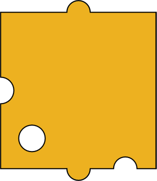
Figure 1: Left, domain with positive and negative features; right, corresponding defeatured geometry.

The simplified geometry obtained by neglecting all the features is called defeatured geometry and denoted by $\Omega_{0}$. It is obtained by cutting off all the positive features and by filling with material the negative ones (see Figure 1-right). For simplicity, we assume it to be a Lipschitz domain as well. In the present work we decide to focus on the negative feature case, hence working with perforated materials. For this reason, the defeatured geometry is defined as

$$\Omega_{0}:=\text{int}\big{(}\overline{\Omega}\cup\{\overline{F},~F\in\mathcal{F}\}\big{)}$$ (2)

For some observations on the extension to the positive feature case, we refer to Remark 3.

Let $\partial\Omega=\Gamma_{\mathrm{D}}\cup\Gamma_{\mathrm{N}}$, with $\Gamma_{\mathrm{D}}\cap\Gamma_{\mathrm{N}}=\emptyset$ and $\Gamma_{D}\neq\emptyset$, and, as in [6], we assume that $\partial F\cap\Gamma_{D}=\emptyset$, $\forall F\in\mathcal{F}$, which means that all the features lie on a Neumann boundary. Finally, let

$$\gamma_{0}:=\bigcup_{F\in\mathcal{F}}(\partial F\setminus\overline{\Gamma_{\mathrm{N}}})\subset\partial\Omega_{0},\quad\text{and}\quad\gamma:=\bigcup_{F\in\mathcal{F}}(\partial F\setminus\overline{\gamma_{0}})\subset\partial\Omega.$$

We set $\gamma_{{}_{F}}={\gamma}|_{{F}}$, such that $\gamma=\bigcup_{F\in\mathcal{F}}\gamma_{{}_{F}}$.

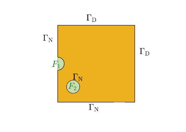
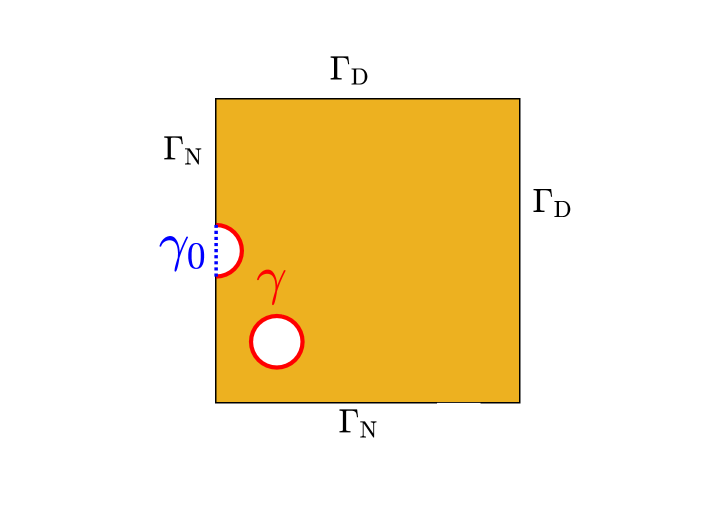
Figure 2: Domain with two negative features and corresponding boundary nomenclature.

As in [7], we do the following separability assumption:

Assumption 1.

The features in $\mathcal{F}$ are separated, i.e.

• For every $F,F^{\prime}\in\mathcal{F}$, $F\neq F^{\prime}$, $\overline{F}\cap\overline{F^{\prime}}=\emptyset$.

• For every $F\in\mathcal{F}$ there exists a sub-domain $\Omega^{F}\subset\Omega$ such that:

  • $\gamma_{{}_{F}}\subset\partial\Omega^{F}$;

  • $|\Omega^{F}|\simeq|\Omega|$, i.e. the measure of the subdomain is comparable to the measure of $\Omega$ and not to the measure of the corresponding feature $F$;

  • the maximum number of superposed subdomains is limited and notably smaller than the total number of features.

As observed in [2], such an assumption is actually pretty weak: the first condition is easily satisfied since, if two features intersect each other they can simply be redefined as a single feature; the second condition allows for features that are arbitrarily close to one another, provided that the number of close features is bounded.

Let us choose as a model problem the Poisson problem on $\Omega$:

$$\begin{cases}-\Delta u=f&\text{in}~\Omega\\ u=g_{\mathrm{D}}&\text{on }\Gamma_{\mathrm{D}}\\ \nabla u\cdot\bm{n}=g&\text{on }\Gamma_{\mathrm{N}},\end{cases}$$ (3)

with $\bm{n}$ being the unitary outward normal of $\Omega$. The variational formulation of Problem (3) reads: find $u\in H^{1}_{g_{\mathrm{D}},\Gamma_{\mathrm{D}}}(\Omega)$ that satisfies, $\forall v\in H^{1}_{0,\Gamma_{\mathrm{D}}}(\Omega)$

$$(\nabla u,\nabla v)_{\Omega}=(f,v)_{\Omega}+\langle g,v\rangle_{\Gamma_{\mathrm{N}}}.$$ (4)

On the defeatured geometry $\Omega_{0}$ we consider instead the defeatured problem

$$\begin{cases}-\Delta u_{0}=f&\text{in}~\Omega_{0}\\ u_{0}=g_{\mathrm{D}}&\text{on }\Gamma_{\mathrm{D}}\\ \nabla u_{0}\cdot\bm{n}_{0}=g&\text{on }\Gamma_{\mathrm{N}}\setminus\gamma\\ \nabla u_{0}\cdot\bm{n}_{0}=g_{0}&\text{on }\gamma_{0},\end{cases}$$ (5)

where $\bm{n}_{0}$ is the unitary outward normal of $\Omega_{0}$ and, by an abuse of notation, $f\in L^{2}(\Omega_{0})$ is a suitable $L^{2}$-extension of $f\in L^{2}(\Omega)$. The variational formulation of Problem (5) reads: find $u_{0}\in H^{1}_{g_{\mathrm{D}},\Gamma_{\mathrm{D}}}(\Omega_{0})$ that satisfies, $\forall v\in H^{1}_{0,\Gamma_{\mathrm{D}}}(\Omega_{0})$

$$(\nabla u_{0},\nabla v)_{\Omega_{0}}=(f,v)_{\Omega_{0}}+\langle g,v\rangle_{\Gamma_{\mathrm{N}}\setminus\gamma}+\langle g_{0},v\rangle_{\gamma_{0}}.$$ (6)

Let $\mathcal{T}_{h}^{0}$ be a non-degenerate simplicial mesh covering $\Omega_{0}$, such that $\overline{\Omega_{0}}=\bigcup_{K\in\mathcal{T}_{h}^{0}}\overline{K}$. Hereby, we suppose that the mesh faces match with the boundaries $\Gamma_{\mathrm{D}}$, $\Gamma_{\mathrm{N}}^{0}:=(\Gamma_{\mathrm{N}}\setminus\gamma)\cup\gamma_{0}$, but we are not asking $\mathcal{T}_{h}^{0}$ to be conforming to the boundaries in $\gamma$. Let us introduce the space

$$Q_{h}(\Omega_{0})=\mathcal{P}_{1}(\mathcal{T}_{h}^{0}):=\left\{q_{h}\in L^{2}(\Omega_{0}):~{q_{h}}|_{{K}}\in\mathcal{P}_{1}(K),~\forall K\in\mathcal{T}_{h}^{0}\right\},$$ (7)

with $\mathcal{P}_{1}(K)$ denoting the space of polynomials of degree at most 1 on $K\in\mathcal{T}_{h}^{0}$, and let

$$V_{h}^{0}(\Omega_{0})=\{v\in\mathcal{C}^{0}(\overline{\Omega_{0}})\cap Q_{h}(\Omega_{0}):{v}|_{{\Gamma_{\mathrm{D}}}}=0\}$$

$$V_{h}(\Omega_{0})=\{v\in\mathcal{C}^{0}(\overline{\Omega_{0}})\cap Q_{h}(\Omega_{0}):{v}|_{{\Gamma_{\mathrm{D}}}}=g_{\mathrm{D}}\}.$$

For the sake of simplicity, we assume $f\in Q_{h}(\Omega_{0})$. Similarly, we assume

$$g_{\mathrm{N}}:=\begin{cases}g&\text{on }\Gamma_{\mathrm{N}}\setminus\gamma\\ g_{0}&\text{on }\gamma_{0}\end{cases}$$ (8)

and $g_{D}$ to be piecewise linear polynomials on the partition induced by $\mathcal{T}_{h}^{0}$ on $\Gamma_{\mathrm{N}}^{0}$ and $\Gamma_{\mathrm{D}}$, respectively. The discrete version of the defeatured problem can then be written as: find $u_{h}^{0}\in V_{h}(\Omega_{0})$ such that

$$(\nabla u_{h}^{0},\nabla v_{h})_{\Omega_{0}}=(f,v_{h})_{\Omega_{0}}+\langle g_{\mathrm{N}},v_{h}\rangle_{\Gamma_{\mathrm{N}}^{0}}\quad\forall v_{h}\in V_{h}^{0}(\Omega_{0}).$$ (9)

Let us split the set of the features in two disjoint subsets $\tilde{\mathcal{F}}$ and $\mathcal{F}^{\star}$, such that $\mathcal{F}=\tilde{\mathcal{F}}\cup\mathcal{F}^{\star}$ and $\tilde{\mathcal{F}}\cap\mathcal{F}^{\star}=\emptyset$, and let us define a partially defeatured geometry as

$${\Omega^{\star}}:=\text{int}\big{(}\overline{\Omega}\cup\{\overline{F},~F\in\tilde{\mathcal{F}}\}\big{)}$$ (10)

The partially defeatured geometry can hence be seen either as a simplification of $\Omega$, in which the features in $\tilde{\mathcal{F}}$ are filled with material and the ones in $\mathcal{F}^{\star}$ are retained, or as a geometrical refinement of $\Omega_{0}$, in which the features in $\mathcal{F}^{\star}$ are included and the ones in $\tilde{\mathcal{F}}$ are neglected. To clarify this second nomenclature, that is often used throughout the paper, we refer to Figure 3. In $\Omega$ (Figure 3(a)) we say that all the features are included, both the ones in $\mathcal{F}^{\star}$ and in $\tilde{\mathcal{F}}$. We set

$$\gamma^{\star}=\bigcup_{F\in\mathcal{F}^{\star}}(\partial F\setminus\overline{\gamma^{\star}_{0}}),\quad\tilde{\gamma}:=\bigcup_{F\in\tilde{\mathcal{F}}}(\partial F\setminus\overline{\tilde{\gamma}_{0}}),$$ (11)

so that $\gamma={\gamma^{\star}}\cup\tilde{\gamma}$. In $\Omega_{0}$ (Figure 3(b)), instead, all the features are neglected. We introduce

$${\gamma}^{\star}_{0}:=\bigcup_{F\in\mathcal{F}^{\star}}(\partial F\setminus\overline{\Gamma_{\mathrm{N}}}),\quad\tilde{\gamma}_{0}:=\bigcup_{F\in\tilde{\mathcal{F}}}(\partial F\setminus\overline{\Gamma_{\mathrm{N}}}),$$ (12)

so that $\gamma_{0}=\gamma_{0}^{\star}\cup\tilde{\gamma}_{0}$. The partially defeatured geometry ${\Omega^{\star}}$ is reported in Figure 3(c): only the features in $\mathcal{F}^{\star}$ are included whereas the features in $\tilde{\mathcal{F}}$ are neglected. We here set $\Gamma_{\mathrm{N}}^{\star}=\Gamma_{\mathrm{N}}^{0}\setminus\gamma_{0}^{\star}$.

We are now interested in defining the partially defeatured problem, which is the problem set on our partial defeatured geometry ${\Omega^{\star}}$. In particular, we consider

$$\begin{cases}-\Delta u^{\star}=f&\text{in}~\Omega^{\star}\\ u^{\star}=g_{\mathrm{D}}&\text{on }\Gamma_{\mathrm{D}}\\ \nabla u^{\star}\cdot\bm{n}^{\star}=g_{\mathrm{N}}&\text{on }\Gamma_{\mathrm{N}}^{\star}\\ \nabla u^{\star}\cdot\bm{n}^{\star}=g&\text{on }\gamma^{\star}\end{cases}$$ (13)

where $\mathbf{{n}^{\star}}$ is the outward unitary normal of $\Omega^{\star}$. The variational formulation of Problem (13) reads: find $u^{\star}\in H^{1}_{g_{\mathrm{D}},\Gamma_{\mathrm{D}}}(\Omega^{\star})$ that satisfies, $\forall v\in H^{1}_{0,\Gamma_{\mathrm{D}}}(\Omega^{\star})$

$$(\nabla u^{\star},\nabla v)_{{\Omega^{\star}}}=(f,v)_{{\Omega^{\star}}}+\langle g,v\rangle_{{\gamma^{\star}}}+\langle g_{\mathrm{N}},v\rangle_{\Gamma_{\mathrm{N}}^{\star}}.$$ (14)

(a) $\Omega$

(b) $\Omega_{0}$

(c) $\Omega^{\star}$

Figure 3: Example of a geometry with four negative features, corresponding totally defeatured geometry and partially defeatured geometry retaining only two features.

Let us now introduce the so called active mesh, defined as the set of elements in $\mathcal{T}_{h}^{0}$ which have a non-empty intersection with the partially defeatured geometry, i.e.

$$\mathcal{A}_{h}:=\{K\in\mathcal{T}_{h}^{0}:~K\cap\Omega^{\star}\neq\emptyset\},$$

and let $\Omega_{{}_{\mathcal{T}}}=\bigcup_{K\in\mathcal{A}_{h}}\overline{K}$ be the domain covered by the elements in $\mathcal{A}_{h}$. Let $h_{K}=\mathrm{diam}(K)$ and $h=\max_{K\in\mathcal{A}_{h}}h_{K}$. For each $K\in\mathcal{A}_{h}$ we define $\gamma_{K}^{\star}=K\cap\gamma^{\star}$, and we introduce the set of cut elements

$$\mathcal{G}_{h}=\{K\in{\mathcal{A}_{h}}:|\gamma_{K}^{\star}|\neq 0\}.$$

Let us now introduce the set

$$Q_{h}(\Omega_{{}_{\mathcal{T}}})=\mathcal{P}_{1}(\mathcal{A}_{h}):=\left\{q_{h}\in L^{2}(\Omega_{{}_{\mathcal{T}}}):~{q_{h}}|_{{K}}\in\mathcal{P}_{1}(K),~\forall K\in\mathcal{A}_{h}\right\},$$ (15)

and

$$V_{h}^{0}(\Omega_{{}_{\mathcal{T}}})=\{v\in C(\overline{\Omega_{{}_{\mathcal{T}}}})\cap Q_{h}(\Omega_{{}_{\mathcal{T}}}):{v}|_{{\Gamma_{\mathrm{D}}}}=0\},$$

$$V_{h}(\Omega_{{}_{\mathcal{T}}})=\{v\in C(\overline{\Omega_{{}_{\mathcal{T}}}})\cap Q_{h}(\Omega_{{}_{\mathcal{T}}}):{v}|_{{\Gamma_{\mathrm{D}}}}=g_{\mathrm{D}}\},$$

and let us consider the discrete problem: find $u_{h}^{\star}\in V_{h}(\Omega_{{}_{\mathcal{T}}})$ such that

$$(\nabla u_{h}^{\star},\nabla v_{h})_{\Omega^{\star}}=(f,v_{h})_{\Omega^{\star}}+\langle g,v_{h}\rangle_{{\gamma^{\star}}}+\langle g_{\mathrm{N}},v_{h}\rangle_{\Gamma_{\mathrm{N}}^{\star}}\quad\forall v_{h}\in V_{h}^{0}(\Omega_{{}_{\mathcal{T}}}),$$ (16)

where, for the sake of simplicity, we assume $g$ to be a piecewise linear polynomial on the partition of ${\gamma^{\star}}$ induced by $\mathcal{A}_{h}$.

3 Error estimator via equilibrated flux reconstruction

Our aim is to control the energy norm of the error $||\nabla(u-u_{h}^{\star})||_{\Omega}$, where $u$ is the solution of (4) and $u_{h}^{\star}$ is the solution of (16). However, we want to achieve this without solving Problem (4). For this reason we propose an a posteriori error estimator defined uniquely on $\Omega^{\star}$ and based on an equilibrated flux reconstructed from $u_{h}^{\star}$. This estimator allows both for standard mesh refinement and for geometric refinement, which consists in choosing, at each step, which features need to be included into the geometry in order to significantly increase the accuracy of the solution. It is directly adapted from [6] in order to handle the case of trimmed elements. Indeed, starting from the totally defeatured geometry $\Omega_{0}$, we aim at gradually including new features without remeshing the domain, but only performing local refinements of the initial non-conforming mesh $\mathcal{T}_{h}^{0}$.

In this section we recall the concept of equilibrated flux reconstruction and we devise a strategy to approximate it on a mesh trimmed by the features in $\mathcal{F}^{\star}$. The a posteriori error analysis based on this flux reconstruction will follow in Section 4.

Let $\bm{\sigma}\in\bm{H}(\text{div},\Omega^{\star})$ be such that

$$\begin{cases}\nabla\cdot\bm{\sigma}=f&\text{ in }\Omega^{\star}\\ \bm{\sigma}\cdot\bm{n}=-g_{\mathrm{N}}&\text{ on }\Gamma_{\mathrm{N}}^{\star}\\ \bm{\sigma}\cdot\bm{n}=-g&\text{ on }{\gamma^{\star}}.\end{cases}$$ (17)

Then, if $u^{\star}\in H^{1}_{g_{\mathrm{D}},\Gamma_{\mathrm{D}}}(\Omega^{\star})$ is the solution of (14), the theorem of Prager and Synge (see [4, 29]) states that, for $v\in H^{1}_{g_{\mathrm{D}},\Gamma_{\mathrm{D}}}({\Omega^{\star}})$,

$$||\nabla(u^{\star}-v)||_{\Omega^{\star}}^{2}+||\nabla u^{\star}+\bm{\sigma}||_{\Omega^{\star}}^{2}=||\nabla v+\bm{\sigma}||_{\Omega^{\star}}^{2}.$$ (18)

Choosing $v=u_{h}^{\star}$ in $\eqref{PragerSynge}$ we obtain

$$||\nabla(u^{\star}-u_{h}^{\star})||_{\Omega^{\star}}^{2}\leq||\nabla u_{h}^{\star}+\bm{\sigma}||_{\Omega^{\star}}^{2},$$

which means that the difference between the numerical flux and a flux $\bm{\sigma}$ satisfying (17) provides a sharp upper bound for the numerical error, with unitary reliability constant.

Equilibrated fluxes are about the cheap construction of such a $\bm{\sigma}$ at a discrete level. In order to build $\bm{\sigma}_{h}$, we resort to a local equilibration procedure directly adapted from [5, 15]. Under this approach, local equilibrated fluxes are built on patches of elements sharing a node, avoiding to solve a global optimization problem and making the method well-suited for parallel implementation.

However, some extra care is needed in order to account for the non-conformity of the mesh with respect to ${\gamma^{\star}}$. Indeed, the Neumann boundary condition is essential for the flux, and it can be imposed strongly on $\Gamma_{\mathrm{N}}^{\star}$ in the definition of the discrete space, since we have assumed that the mesh is conforming to this portion of the boundary. The Neumann boundary condition on ${\gamma^{\star}}$ has instead to be imposed weakly: we hence decide to work in a CutFEM framework, adopting a Nitsche method as proposed in [30] for the case of the mixed formulation of the Darcy problem in the unfitted case. For a flux recovery for CutFEM in the case of Dirichlet boundary conditions we refer the reader to [13], which resorts however to a different local equilibration procedure.

Remark 1.

Let us remark that the non conformity of the mesh with respect to $\tilde{\gamma}$ is instead not relevant when building $\bm{\sigma}_{h}$, since the equilibrated flux is reconstructed on the partially defeatured geometry ${\Omega^{\star}}$, which is blind to the features in $\tilde{\mathcal{F}}$.

In the following, we denote by ${\mathscr{N}_{h}}$ and $\mathscr{E}_{h}$ respectively the set of vertices and edges in the active mesh ${\mathcal{A}_{h}}$. In particular the set of vertices is decomposed into $\mathscr{N}_{h}^{\mathrm{ext}}$ and $\mathscr{N}_{h}^{\mathrm{int}}$, corresponding respectively to vertices lying on $\Gamma_{\mathrm{N}}^{\star}$ and inside $\Omega_{0}$. Let us remark that the nodes belonging to $\mathcal{A}_{h}$ but lying inside a feature will still belong to $\mathscr{N}_{h}^{\mathrm{int}}$.

Let us consider a vertex $\bm{a}\in\mathscr{N}_{h}$ and let us denote by ${\omega_{\bm{a}}}$ the open patch of elements of $\mathcal{A}_{h}$ sharing that node, and by $\psi_{\bm{a}}$ the hat function in $Q_{h}(\Omega_{{}_{\mathcal{T}}})\cap H^{1}(\Omega_{{}_{\mathcal{T}}})$ taking value 1 in vertex $\bm{a}$ and 0 in all the other vertices. Let ${\partial\omega_{\bm{a}}}$ be the boundary of ${\omega_{\bm{a}}}$, and let us define (see Figure 4) ${\partial\omega_{\bm{a}}^{0}}\subseteq{\partial\omega_{\bm{a}}}$ as

$${\partial\omega_{\bm{a}}^{0}}=\{\bm{x}\in\partial{\omega_{\bm{a}}}~:\psi_{\bm{a}}(\bm{x})=0\},$$

and $\partial\omega_{\bm{a}}^{\psi}=\partial{\omega_{\bm{a}}}\setminus{\partial\omega_{\bm{a}}^{0}}$.

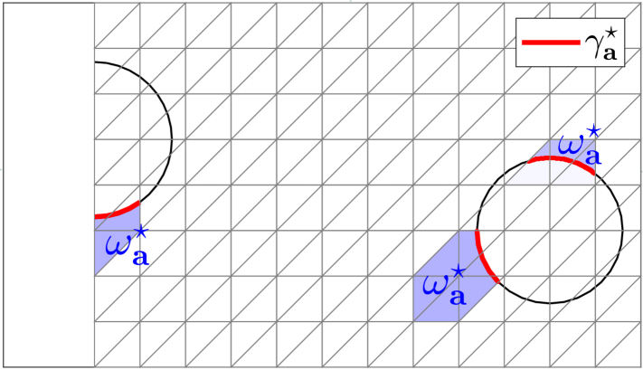
Figure 4: Nomenclature for patch boundaries

Let us now introduce the space

$$\bm{M}_{h}({\omega_{\bm{a}}}):=\left\{\bm{v}_{h}\in\bm{H}(\text{div},{\omega_{\bm{a}}}):~{\bm{v}_{h}}|_{{K}}\in[\mathcal{P}_{1}(K)]^{d}+\bm{x}\mathcal{P}_{1}(K),~\forall K\in{\omega_{\bm{a}}}\right\},$$

which is the Raviart-Thomas finite element space of order 1 on ${\omega_{\bm{a}}}$, and let

$$\bm{M}_{h}^{\bm{a},0}=\left\{\bm{v}_{h}\in\bm{M}_{h}({\omega_{\bm{a}}}):~\bm{v}_{h}\cdot\bm{n}_{{\omega_{\bm{a}}}}=0\text{ on }{\partial\omega_{\bm{a}}^{0}}\right\}$$

and $Q_{h}({\omega_{\bm{a}}})$ be the restriction of $Q_{h}(\Omega_{{}_{\mathcal{T}}})$ to ${\omega_{\bm{a}}}$. We then define

$$\bm{M}_{h}^{\bm{a}} :=\begin{cases}\bm{M}_{h}^{\bm{a},0}&\text{ if }\bm{a}\in\mathscr{N}_{h}^{\mathrm{int}}\\ \big{\{}\bm{v}_{h}\in\bm{M}_{h}({\omega_{\bm{a}}}):~\bm{v}_{h}\cdot\bm{n}_{{\omega_{\bm{a}}}}=0\text{ on }{\partial\omega_{\bm{a}}^{0}}\\ \hskip 76.82234pt\bm{v}_{h}\cdot\bm{n}_{{\omega_{\bm{a}}}}=-{\psi_{\bm{a}}}g_{\mathrm{N}}\text{ on }{\partial\omega_{\bm{a}}^{\psi}}\cap\Gamma_{\mathrm{N}}^{0}\}&\text{ if }\bm{a}\in{\mathscr{N}_{h}}^{\mathrm{ext}},\end{cases}$$ (19)

$$Q_{h}^{\bm{a}} :=\begin{cases}\big{\{}q_{h}\in Q_{h}({\omega_{\bm{a}}}):(q_{h},1)_{{\omega_{\bm{a}}}}=0\big{\}}&\text{ if }\bm{a}\in{\mathscr{N}_{h}}^{\mathrm{int}}\text{ or }\bm{a}\in\text{int}(\overline{\Gamma_{\mathrm{N}}^{0}})\\[3.99994pt] Q_{h}({\omega_{\bm{a}}})&\text{ if }\bm{a}\in{\mathscr{N}_{h}}^{\mathrm{ext}}\text{ and }\bm{a}\notin\text{int}(\overline{\Gamma_{\mathrm{N}}^{0}}),\end{cases}$$ (20)

where $\bm{n}_{\omega_{\bm{a}}}$ is the outward unit normal of ${\omega_{\bm{a}}}$.

For the sake of compactness, let us set (see Figure 4)

$$h_{\bm{a}}=\max_{K\subset{\omega_{\bm{a}}}}h_{K},\quad\omega_{\bm{a}}^{\star}={\omega_{\bm{a}}}\cap\Omega^{\star},\quad\gamma_{\bm{a}}^{\star}={\gamma^{\star}}\cap{\omega_{\bm{a}}}.$$

For $p\in\{0,1\}$, let us then introduce the bilinear forms $m_{\bm{a}}:\bm{M}_{h}^{\bm{a}}\times\bm{M}_{h}^{\bm{a}}\rightarrow\mathbb{R}$ and $b_{\bm{a}}^{p}:\bm{M}_{h}^{\bm{a}}\times Q_{h}^{\bm{a}}\rightarrow\mathbb{R}$ such that

$$m_{\bm{a}}(\bm{\rho}_{h},\bm{v}_{h}):=(\bm{\rho}_{h},\bm{v}_{h})_{{\omega}_{\bm{a}}^{\star}}+\frac{1}{h_{\bm{a}}}\langle\bm{\rho}_{h}\cdot\bm{n},\bm{v}_{h}\cdot\bm{n}\rangle_{\gamma_{\bm{a}}^{\star}}$$

$$b_{\bm{a}}^{p}(\bm{v}_{h},q_{h}):=(q_{h},\nabla\cdot\bm{v}_{h})_{{\omega}_{\bm{a}}^{\star}}-p\langle q_{h},\bm{v}_{h}\cdot\bm{n}\rangle_{\gamma_{\bm{a}}^{\star}}$$

and the linear operators $L_{\bm{a}}:\bm{M}_{h}^{\bm{a}}\rightarrow\mathbb{R}$ and $R_{\bm{a}}^{p}:Q_{h}^{\bm{a}}\rightarrow\mathbb{R}$ such that

$$L_{\bm{a}}(\bm{v_{h}}):=-(\psi_{\bm{a}}\nabla u_{h}^{\star},\bm{v}_{h})_{{\omega}_{\bm{a}}^{\star}}-\frac{1}{h_{\bm{a}}}\langle\psi_{\bm{a}}g,\bm{v}_{h}\cdot\bm{n}\rangle_{\gamma_{\bm{a}}^{\star}}$$ (21)

$$R_{\bm{a}}^{p}(q_{h}):=(\psi_{\bm{a}}f-\nabla\psi_{\bm{a}}\cdot\nabla u_{h}^{\star},q_{h})_{{\omega}_{\bm{a}}^{\star}}+p\langle\psi_{\bm{a}}g,q_{h}\rangle_{\gamma_{\bm{a}}^{\star}},$$ (22)

On each patch we then solve a problem in the form: find $(\bm{\sigma}_{h}^{\bm{a}},\lambda_{h}^{\bm{a}})\in\bm{M}_{h}^{\bm{a}}\times Q_{h}^{\bm{a}}$ such that

$$\begin{cases}m_{\bm{a}}(\bm{\sigma}_{h}^{\bm{a}},\bm{v}_{h})-b_{\bm{a}}^{1}(\bm{v}_{h},\lambda_{h}^{\bm{a}})=L_{\bm{a}}(\bm{v}_{h})&\forall\bm{v}_{h}\in\bm{M}_{h}^{\bm{a}}\\ \hskip 62.59596ptb_{\bm{a}}^{p}(\bm{\bm{\sigma}_{h}^{\bm{a}}},q_{h})=R_{\bm{a}}^{p}(q_{h})&\forall q_{h}\in Q_{h}^{\bm{a}},\end{cases}$$ (23)

Finally, the flux reconstruction is built by summing all the local contributions, i.e.

$$\bm{\sigma}_{h}=\sum_{\bm{a}\in\mathscr{N}_{h}}\bm{\sigma}_{h}^{\bm{a}}.$$

We now analyze the properties of $\bm{\sigma}_{h}$ in different scenarios, in particular when $\mathcal{F}^{\star}$ is or not an empty set. For any $\bm{a}\in\mathscr{N}_{h}$ we denote by $\overline{q_{h}}^{\omega_{\bm{a}}}$ the average of $q_{h}\in Q_{h}({\omega_{\bm{a}}})$ on ${\omega_{\bm{a}}}$. Setting $c_{\bm{a}}=-\overline{q_{h}}^{\omega_{\bm{a}}}$, we have that $q_{h}+c_{\bm{a}}\in Q_{h}^{\bm{a}}$. The second equation in (23) can hence be rewritten as

$$b_{\bm{a}}^{p}(\bm{\bm{\sigma}_{h}^{\bm{a}}},q_{h}+c_{\bm{a}})=R_{\bm{a}}^{p}(q_{h}+c_{\bm{a}})\qquad\forall q_{h}\in Q_{h}({\omega_{\bm{a}}}).$$ (24)

If $\mathcal{F}^{\star}=\emptyset$, i.e. none of the features in $\mathcal{F}$ is included into the geometry, then it is possible to prove that, given the regularity assumptions on $f$, the flux $\bm{\sigma}_{h}$ reconstructed from $u_{h}^{\star}=u_{h}^{0}$ is such that $||\nabla\cdot\bm{\sigma}_{h}-f||_{K}=0$, $\forall K\in\mathcal{A}_{h}=\mathcal{T}_{h}^{0}$. Equation (24) can indeed be written, for any $\bm{a}\in\mathscr{N}_{h}$, as

$$(\nabla\cdot\bm{\sigma}_{h}^{\bm{a}},q_{h}+c_{\bm{a}})_{{\omega_{\bm{a}}}}=({\psi_{\bm{a}}}f-\nabla\psi_{\bm{a}}\cdot\nabla u_{h}^{0},q_{h}+c_{\bm{a}})_{{\omega_{\bm{a}}}}\qquad\forall q_{h}\in Q_{h}({\omega_{\bm{a}}}).$$ (25)

Let us now observe that, according to (9), we have that

$$(\nabla{\psi_{\bm{a}}}\cdot\nabla u_{h}^{0},1)_{{\omega_{\bm{a}}}}=({\psi_{\bm{a}}}f,1)_{{\omega_{\bm{a}}}}+\langle{\psi_{\bm{a}}}g_{\mathrm{N}},1\rangle_{\partial\omega_{\bm{a}}^{\psi}\cap\Gamma_{\mathrm{N}}^{0}}$$ (26)

while, by the divergence theorem,

$$(\nabla\cdot\bm{\sigma}_{h}^{\bm{a}},1)_{{\omega_{\bm{a}}}}=\langle\bm{\sigma}_{h}^{\bm{a}}\cdot\bm{n}_{\omega_{\bm{a}}},1\rangle_{\partial\omega_{\bm{a}}^{\psi}\cap\Gamma_{\mathrm{N}}^{0}}.$$ (27)

Since the Neumann condition is strongly imposed on $\partial\omega_{\bm{a}}^{\psi}\cap\Gamma_{\mathrm{N}}^{0}$, we can rewrite (25) as

$$(\nabla\cdot\bm{\sigma}_{h}^{\bm{a}},q_{h})_{{\omega_{\bm{a}}}}=({\psi_{\bm{a}}}f-\nabla\psi_{\bm{a}}\cdot\nabla u_{h}^{0},q_{h})_{{\omega_{\bm{a}}}},\quad\forall q_{h}\in Q_{h}({\omega_{\bm{a}}})$$ (28)

Let us consider $K\in\mathcal{T}_{h}^{0}$ and let us denote its nodes by $\mathscr{N}_{h}(K)$. Since the polynomials in $Q_{h}({\omega_{\bm{a}}})$ are discontinuous, then (28) holds also for $q_{h}\in\mathcal{P}_{1}(K)$. We hence have that

$$(\nabla\cdot\bm{\sigma}_{h},q_{h})_{K} =\sum_{\bm{a}\in\mathscr{N}_{h}(K)}(\nabla\cdot\bm{\sigma}_{h}^{\bm{a}},q_{h})_{K}=\sum_{\bm{a}\in\mathscr{N}_{h}(K)}({\psi_{\bm{a}}}f,q_{h})_{K}=(f,q_{h})_{K}\quad\forall q_{h}\in\mathcal{P}_{1}(K),$$ (29)

where we have also exploited the fact that ${\psi_{\bm{a}}}$ is a partition of unity and hence $\sum_{\bm{a}\in\mathscr{N}_{h}(K)}\nabla{\psi_{\bm{a}}}=0$.

In the second case, when $\mathcal{F}^{\star}\neq\emptyset$, the flux reconstructed from $u_{h}^{\star}$ is instead a weakly equilibrated flux reconstruction, due to the error introduced by the weak imposition of the Neumann boundary condition on ${\gamma^{\star}}$. Indeed $||\bm{\sigma}_{h}\cdot\bm{n}+g||_{{\gamma^{\star}}}$ will not be zero, and also the mass balance may be polluted, ending up in some elements for which $||\nabla\cdot\bm{\sigma}_{h}-f||_{K\cap{\Omega^{\star}}}\neq 0$.

Let us start from the case $p=0$, i.e. from the asymmetric version of the saddle-point problem (23). For any $q_{h}\in Q_{h}({\omega_{\bm{a}}})$, equation (24) can be rewritten as

$$(\nabla\cdot\bm{\sigma}_{h}^{\bm{a}},q_{h}+c_{\bm{a}})_{{\omega}_{\bm{a}}^{\star}}=({\psi_{\bm{a}}}f-\nabla\psi_{\bm{a}}\cdot\nabla u_{h}^{\star},q_{h}+c_{\bm{a}})_{{\omega}_{\bm{a}}^{\star}}.$$ (30)

According to (16), we have that

$$(\nabla{\psi_{\bm{a}}}\cdot\nabla u_{h}^{\star},1)_{{\omega}_{\bm{a}}^{\star}}=({\psi_{\bm{a}}}f,1)_{{\omega}_{\bm{a}}^{\star}}+\langle{\psi_{\bm{a}}}g,1\rangle_{\gamma_{\bm{a}}^{\star}}+\langle{\psi_{\bm{a}}}g_{\mathrm{N}},1\rangle_{\partial\omega_{\bm{a}}^{\psi}\cap\Gamma_{\mathrm{N}}^{\star}},$$ (31)

while, by the divergence theorem,

$$(\nabla\cdot\bm{\sigma}_{h}^{\bm{a}},1)_{{\omega}_{\bm{a}}^{\star}}=\langle\bm{\sigma}_{h}^{\bm{a}}\cdot\bm{n},1\rangle_{\gamma_{\bm{a}}^{\star}}+\langle\bm{\sigma}_{h}^{\bm{a}}\cdot\bm{n}_{\omega_{\bm{a}}},1\rangle_{\partial\omega_{\bm{a}}^{\psi}\cap\Gamma_{\mathrm{N}}^{\star}}.$$ (32)

Exploiting the fact that the Neumann boundary condition is imposed in strong form on the whole ${\partial\omega_{\bm{a}}^{\psi}}\cap\Gamma_{\mathrm{N}}^{0}$ we can rewrite (30) as

$$(\nabla\cdot\bm{\sigma}_{h}^{\bm{a}},q_{h})_{{\omega}_{\bm{a}}^{\star}}+\langle\bm{\sigma}_{h}^{\bm{a}}\cdot\bm{n}+{\psi_{\bm{a}}}g,c_{\bm{a}}\rangle_{\gamma_{\bm{a}}^{\star}}=({\psi_{\bm{a}}}f-\nabla\psi_{\bm{a}}\cdot\nabla u_{h}^{\star},q_{h})_{{\omega}_{\bm{a}}^{\star}},\quad\forall q_{h}\in Q_{h}({\omega_{\bm{a}}})$$ (33)

which holds also for $q_{h}\in\mathcal{P}_{1}(K)$, since the polynomials in $Q_{h}({\omega_{\bm{a}}})$ are discontinuous. We hence have that for any $K\in\mathcal{A}_{h}$ and for any $q_{h}\in\mathcal{P}_{1}(K)$

$$(\nabla\cdot\bm{\sigma}_{h},q_{h})_{K\cap{\Omega^{\star}}}=\hskip-8.5359pt\sum_{\bm{a}\in\mathscr{N}_{h}(K)}(\nabla\cdot\bm{\sigma}_{h}^{\bm{a}},q_{h})_{K\cap{\Omega^{\star}}} =(f,q_{h})_{K\cap{\Omega^{\star}}}-\hskip-8.5359pt\sum_{\bm{a}\in\mathscr{N}_{h}(K)}(\bm{\sigma}_{h}^{\bm{a}}\cdot\bm{n}+{\psi_{\bm{a}}}g,c_{\bm{a}})_{\gamma_{\bm{a}}^{\star}}$$ (34)

where we have exploited the fact that $\sum_{\bm{a}\in\mathscr{N}_{h}(K)}\nabla{\psi_{\bm{a}}}=0$.

Things are instead different if $p=1$. Indeed, for any $q_{h}\in Q_{h}({\omega_{\bm{a}}})$ equation (24) can be rewritten as

$$(\nabla\cdot\bm{\sigma}_{h}^{\bm{a}},q_{h}+c_{\bm{a}})_{{\omega}_{\bm{a}}^{\star}}-\langle\bm{\sigma}_{h}^{\bm{a}}\cdot\bm{n}+{\psi_{\bm{a}}}g,q_{h}+c_{\bm{a}}\rangle_{\gamma_{\bm{a}}^{\star}}=({\psi_{\bm{a}}}f-\nabla\psi_{\bm{a}}\cdot\nabla u_{h}^{\star},q_{h}+c_{\bm{a}})_{{\omega}_{\bm{a}}^{\star}}$$ (35)

while (31) and (32) are still holding. This means that (35) simply reduces to

$$(\nabla\cdot\bm{\sigma}_{h}^{\bm{a}},q_{h})_{{\omega}_{\bm{a}}^{\star}}-\langle\bm{\sigma}_{h}^{\bm{a}}\cdot\bm{n}+{\psi_{\bm{a}}}g,q_{h}\rangle_{\gamma_{\bm{a}}^{\star}}=({\psi_{\bm{a}}}f-\nabla\psi_{\bm{a}}\cdot\nabla u_{h}^{\star},q_{h})_{{\omega}_{\bm{a}}^{\star}}\quad\forall q_{h}\in Q_{h}({\omega_{\bm{a}}}),$$

and that, for any $K\in\mathcal{A}_{h}$ and $q_{h}\in\mathcal{P}_{1}(K)$

$$(\nabla\cdot\bm{\sigma}_{h},q_{h})_{K\cap{\Omega^{\star}}} =\sum_{\bm{a}\in\mathscr{N}_{h}(K)}(\nabla\cdot\bm{\sigma}_{h}^{\bm{a}},q_{h})_{K\cap{\Omega^{\star}}}=(f,q_{h})_{K\cap{\Omega^{\star}}}+\langle\bm{\sigma}_{h}\cdot\bm{n}+g,q_{h}\rangle_{\gamma_{K}^{\star}}.$$ (36)

Let us remark that, in (34) the mass is not completely balanced in all the elements belonging to a cut patch, i.e. a patch ${\omega_{\bm{a}}}$ such that $|\gamma_{\bm{a}}^{\star}|\neq 0$. On the contrary, in (36), the mass is not balanced only in the elements for which $|\gamma_{K}^{\star}|\neq 0$, i.e. only for $K\in\mathcal{G}_{h}$. This means that, for $p=1$, and since we have assumed that $f\in Q_{h}(\Omega_{0})$,

$$||\nabla\cdot\bm{\sigma}_{h}-f||_{K}=0\quad\forall K\in\mathcal{A}_{h}\setminus\mathcal{G}_{h}.$$ (37)

Remark 2.

It is well known that the weak imposition of essential boundary conditions in CutFEM may require stabilization in presence of very small cuts [10]. Let $v:\Omega_{{}_{\mathcal{T}}}\rightarrow\mathbb{R}$ be smooth enough and let us define the jump as

$$\llbracket v\rrbracket_{e}:={v}|_{{K_{1}}}-{v}|_{{K_{2}}},$$

with $e=\partial K_{1}\cap\partial K_{2}$. Let us then introduce for $\bm{a}\in\mathscr{N}_{h}$,

$$\mathscr{E}_{h,\bm{a}}:=\{e\in\mathscr{E}_{h}\text{ such that }~\exists K\in\mathcal{A}_{h},~K\subset{\omega_{\bm{a}}}:~e\subset\partial K\},\vskip 8.5359pt$$

and let $\mathscr{E}_{h,\bm{a}}^{\mathrm{int}}:=\{e\in\mathscr{E}_{h,\bm{a}}\text{ such that }~e\nsubseteq\partial{\omega_{\bm{a}}}\}.$ Finally we set

$$\mathscr{E}_{h,\bm{a}}^{\mathcal{G}}:=\{e\in\mathscr{E}_{h,\bm{a}}^{\mathrm{int}}\text{ such that }~\exists K\in\mathcal{G}_{h}:~e\subset\partial K\}$$

and we define the bilinear forms ([10, 11]) $\bm{j}_{h}:\bm{M}_{h}^{\bm{a}}\times\bm{M}_{h}^{\bm{a}}\rightarrow\mathbb{R}$, $j_{h}:Q_{h}^{\bm{a}}\times Q_{h}^{\bm{a}}\rightarrow\mathbb{R}$ such that

$$\bm{j}_{\bm{a}}(\bm{\rho}_{h},\bm{v}_{h}):=\beta_{1}\sum_{e\in\mathscr{E}_{h,\bm{a}}^{\mathcal{G}}}\Big{[}h_{\bm{a}}(\llbracket\bm{\rho}_{h}\rrbracket_{e},\llbracket\bm{v}_{h}\rrbracket_{e})_{e}+h_{\bm{a}}^{3}(\llbracket\nabla\bm{\rho}_{h}\cdot\bm{n}_{e}\rrbracket_{e},\llbracket\nabla\bm{v}_{h}\cdot\bm{n}_{e}\rrbracket_{e})_{e}\Big{]}$$ (38)

$$j_{\bm{a}}(\mu_{h},q_{h}):=\beta_{2}\sum_{e\in\mathscr{E}_{h,\bm{a}}^{\mathcal{G}}}\Big{[}\frac{1}{h_{\bm{a}}}(\llbracket\mu_{h}\rrbracket_{e},\llbracket q_{h}\rrbracket_{e})_{e}+h_{\bm{a}}(\llbracket\nabla\mu_{h}\cdot\bm{n}_{e}\rrbracket_{e},\llbracket\nabla q_{h}\cdot\bm{n}_{e}\rrbracket_{e})_{e}\Big{]},$$ (39)

with $\beta_{1},\beta_{2}>0$ and $\bm{n}_{e}$ denoting the unit normal vector to $e$, whose orientation is fixed. The stabilized version of Problem (23) then reads as: find $(\bm{\sigma}_{h}^{\bm{a}},\lambda_{h}^{\bm{a}})\in\bm{M}_{h}^{\bm{a}}\times Q_{h}^{\bm{a}}$ such that

$$\begin{cases}m_{\bm{a}}(\bm{\sigma}_{h}^{\bm{a}},\bm{v}_{h})-b_{\bm{a}}^{1}(\bm{v}_{h},\lambda_{h}^{\bm{a}})+\bm{j}_{\bm{a}}(\bm{\sigma}_{h},\bm{v}_{h})=L_{\bm{a}}(\bm{v}_{h})&\forall\bm{v}_{h}\in\bm{M}_{h}^{\bm{a}}\\[6.00006pt] \hskip 62.59596ptb_{\bm{a}}^{p}(\bm{\bm{\sigma}_{h}^{\bm{a}}},q_{h})-j_{\bm{a}}(\lambda_{h}^{\bm{a}},q_{h})=R_{\bm{a}}^{p}(q_{h})&\forall q_{h}\in Q_{h}^{\bm{a}}.\end{cases}$$ (40)

The scalar stabilization term introduced in the second equation is however likely to further pollute mass balance, not only on cut elements but on all the cut patches. Using a projection-based stabilization only on badly cut patches (see for example [30]) would allow to reduce the number of elements on which this additional error is introduced, but it might also affect the monotonicity of the estimator proposed in the next section. Indeed, assuming to use the estimator in an adaptive procedure, badly cut elements are very likely to appear and disappear as the mesh changes, introducing extra contributions to the estimator only at certain steps. Divergence preserving techniques have been proposed in [19], requiring however the evaluation of higher order derivatives, and hence increasing the computational effort required to compute $\bm{\sigma}_{h}$.

Let us recall that $\bm{\sigma}_{h}$ is not the primal variable of our problem: it is computed only with the aim of building the estimator, so it is of interest to keep its computation as cheap as possible. For this reason, badly cut elements could also be simply neglected, allowing to avoid the case in which an element that has barely an active part, strongly affects the total estimator only due to stabilization. Further remarks on this aspect can be found in Section 6.

Remark 3.

In the present work we decided to focus on the negative feature case and on the challenges posed by the presence of cut elements. In the case of a positive feature included into the partially defeatured geometry, the equilibrated flux reconstruction in the feature and in the rest of the domain could be computed separately, provided that proper coupling conditions are defined at the interface.

What is interesting to remark is that, as reported in [6] (see also [9]), positive features with complex shapes are often treated by introducing a bounding box having the simplest possible shape, meshing the bounding box instead of the actual feature and computing the flux reconstruction on that mesh, which is blind to the feature boundary. Since a positive feature is actually a negative feature from its bounding box perspective, all the analysis that was carried out until now can easily be exploited.

4 A posteriori error analysis

In this section we propose a reliable estimator for the error $||\nabla(u-u_{h}^{\star})||_{\Omega}$, based on the (weakly) equilibrated flux defined above.

For $F\in\tilde{\mathcal{F}}$ let ${\tilde{\gamma}_{F}}:=\tilde{\gamma}\cap\partial F$ and $\tilde{\gamma}_{{0,F}}=\tilde{\gamma}_{0}\cap F$, so that $\tilde{\gamma}=\bigcup_{F\in\tilde{\mathcal{F}}}{\tilde{\gamma}_{F}}$ and $\tilde{\gamma}_{0}=\bigcup_{F\in\tilde{\mathcal{F}}}{\tilde{\gamma}_{0,F}}$. For every $F\in\tilde{\mathcal{F}}$ let ${\bm{\sigma}}|_{{F}}\in\bm{H}(\text{div},F)$ be the solution of

$$\begin{cases}\nabla\cdot{\bm{\sigma}}|_{{F}}=f&\text{ in }F\\[3.00003pt] {\bm{\sigma}}|_{{F}}\cdot\bm{n_{0}}=-g_{0}&\text{ on }\tilde{\gamma}_{0,F}\\[3.00003pt] {\bm{\sigma}}|_{{F}}\cdot\bm{n_{F}}=-\bm{\sigma}\cdot\bm{n}&\text{ on }\tilde{\gamma}_{F},\end{cases}$$ (41)

where $\bm{\sigma}\in\bm{H}(\text{div},{\Omega^{\star}})$ is a generic flux satisfying (17). Vectors $\bm{n_{F}}=-\bm{n}$ and $\bm{n_{0}}$ are the unitary outward normals of $F$ on $\tilde{\gamma}_{F}$ and $\tilde{\gamma}_{0,F}$, respectively. Omitting, by an abuse of notation, the explicit restriction of $\bm{\sigma}$ to $F$, we define for every $F\in\tilde{\mathcal{F}}$, the quantity

$$d_{F}:=g+\bm{\sigma}\cdot\bm{n}\quad\text{on }\tilde{\gamma}_{F},$$

which is the error between the Neumann datum $g$ on ${\tilde{\gamma}_{F}}$ and the normal trace of $\bm{\sigma}$. Similarly we define

$$d_{F}^{h}:=g+\bm{\sigma}_{h}\cdot\bm{n}\quad\text{on }\tilde{\gamma}_{F},$$

where $\bm{\sigma}_{h}$ is a (weakly) equilibrated flux reconstructed from $u_{h}^{\star}$ as detailed in Section 3, choosing $p=1$ in (23). Denoting by $\overline{d_{F}}^{\tilde{\gamma}_{F}}$ and $\overline{d_{F}^{h}}^{\tilde{\gamma}_{F}}$ the average, respectively, of $d_{F}$ and $d_{F}^{h}$ over ${\tilde{\gamma}_{F}}$ we define

$$\mathcal{E}_{F}^{2}:=|{\tilde{\gamma}_{F}}|\big{|}\big{|}d_{F}^{h}-\overline{d_{F}^{h}}^{\tilde{\gamma}_{F}}\big{|}\big{|}_{{\tilde{\gamma}_{F}}}^{2}+c_{{\tilde{\gamma}_{F}}}^{2}|{\tilde{\gamma}_{F}}|^{2}\big{|}\overline{d_{F}}^{\tilde{\gamma}_{F}}\big{|}^{2},$$ (42)

with $c_{{\tilde{\gamma}_{F}}}$ defined according to (1). Let us remark that $\overline{d_{F}}^{\tilde{\gamma}_{F}}$ actually depends only on the choice of the extension of $f$ inside $F$ and on the choice of $g_{0}$. Indeed, according to (41),

$$\overline{d_{F}}^{\tilde{\gamma}_{F}}=\frac{1}{|\tilde{\gamma}_{F}|}(g+\bm{\sigma}\cdot\bm{n},1)_{\tilde{\gamma}_{F}}=\frac{1}{|\tilde{\gamma}_{F}|}\big{[}(g,1)_{\tilde{\gamma}_{F}}-(f,1)_{F}-(g_{0},1)_{\tilde{\gamma}_{0,F}}\big{]},$$

so that a proper choice of the data allows us to get rid of the second term in $\mathcal{E}_{F}^{2}$.

For each $K\in\mathcal{A}_{h}$ we also define

$$\mathcal{E}_{\mathrm{div}}^{K}:=h_{K}||f-\nabla\cdot\bm{\sigma}_{h}||_{K\cap{\Omega^{\star}}}\qquad\mathcal{E}_{\sigma}^{K}:=||\bm{\sigma}_{h}+\nabla u_{h}^{\star}||_{K\cap{\Omega^{\star}}}.$$ (43)

$$\mathcal{E}_{\mathrm{g}}^{K}:=h_{K}^{\frac{1}{2}}(||g+\bm{\sigma}_{h}\cdot\bm{n}||_{\gamma_{K}^{\star}}^{2}\big{)}^{\frac{1}{2}}$$ (44)

We now state and prove the proposition establishing our a posteriori bound under the following technical assumption ([7]):

Assumption 2.

For every $F\in\tilde{\mathcal{F}}$ let $h_{F}:=\mathrm{diam}(F)$ and $h_{F}^{\mathrm{min}}:=\min\{{h_{K}:K\in\mathcal{A}_{h},~K\cap F\neq\emptyset}\}$. Then we assume that $h_{F}\lesssim h_{F}^{\mathrm{min}}$, which actually means that the number of elements covering a non-included feature can not grow indefinitely.

For some observations on this assumption we refer the reader to Remark 6 in Section 5.

Proposition 1.

Let $u$ be the solution to (4) and $u_{h}^{\star}$ the solution to (16). Then, choosing $p=1$ in (23), and under Assumption 2, there exist three constants $\alpha_{1},\alpha_{2},\alpha_{3}>0$ independent on the mesh size $h$ and on the sizes of the features, such that

$$||\nabla(u-u_{h}^{\star})||_{\Omega}\leq\Big{(}\sum_{K\in\mathcal{G}_{h}}\alpha_{1}(\mathcal{E}_{\mathrm{div}}^{K})^{2}\Big{)}^{\frac{1}{2}}+\Big{(}\sum_{K\in\mathcal{G}_{h}}\alpha_{2}(\mathcal{E}_{\mathrm{g}}^{K})^{2}\Big{)}^{\frac{1}{2}}+\Big{(}\sum_{K\in\mathcal{A}_{h}}(\mathcal{E}_{\sigma}^{K})^{2}\Big{)}^{\frac{1}{2}}+\Big{(}\sum_{F\in\tilde{\mathcal{F}}}\alpha_{3}\mathcal{E}_{F}^{2}\Big{)}^{\frac{1}{2}}$$

Proof.

Let $v\in H_{0,\Gamma_{\mathrm{D}}}(\Omega)$. Adding and subtracting $(\bm{\sigma}_{h},\nabla v)_{\Omega}$, and exploiting (4) we have that

$$(\nabla(u-u_{h}^{\star}),\nabla v)_{\Omega} =(\nabla u+\bm{\sigma}_{h},\nabla v)_{\Omega}-(\nabla u_{h}^{\star}+\bm{\sigma}_{h},\nabla v)_{\Omega}$$

$$=(f-\nabla\cdot\bm{\sigma}_{h},v)_{\Omega}+\langle g+\bm{\sigma}_{h}\cdot\bm{n},v\rangle_{{\gamma^{\star}}}+\langle g+\bm{\sigma}_{h}\cdot\bm{n},v\rangle_{\tilde{\gamma}}$$

$$\quad-(\nabla u_{h}^{\star}+\bm{\sigma}_{h},\nabla v)_{\Omega}.$$ (45)

Let $\mathbf{E}^{0}:H_{0,\Gamma_{\mathrm{D}}}(\Omega)\rightarrow H_{0,\Gamma_{\mathrm{D}}}(\Omega_{0})$ be a generalized Stein extension operator, such that $\forall v\in H_{0,\Gamma_{\mathrm{D}}}(\Omega)$

$$||\nabla\mathbf{E}^{0}(v)||_{\Omega_{0}}\lesssim||\nabla v||_{\Omega}.$$ (46)

For the construction of $\mathbf{E}^{0}$ we refer the reader to [31], in which such extension operators are built for a large class of domains, and in particular for domains characterized by separated geometrical details of smaller scale. Let $v_{0}=\mathbf{E}^{0}(v)\in H_{0,\Gamma_{\mathrm{D}}}(\Omega_{0})$, and let us rewrite (45) as:

$$(\nabla(u-u_{h}^{\star}),\nabla v)_{\Omega} =(f-\nabla\cdot\bm{\sigma}_{h},v_{0})_{\Omega^{\star}}+\langle g+\bm{\sigma}_{h}\cdot\bm{n},v_{0}\rangle_{{\gamma^{\star}}}-(\nabla u_{h}^{\star}+\bm{\sigma}_{h},\nabla v_{0})_{\Omega}$$

$$\quad+\sum_{F\in\mathcal{\tilde{\mathcal{F}}}}\big{[}\langle g+\bm{\sigma}_{h}\cdot\bm{n},v_{0}\rangle_{{\tilde{\gamma}_{F}}}-(f-\nabla\cdot\bm{\sigma}_{h},v_{0})_{F}\big{]}=\mathrm{I}+\mathrm{II}+\mathrm{III},$$ (47)

with

$$\mathrm{I}=(f-\nabla\cdot\bm{\sigma}_{h},v_{0})_{\Omega^{\star}}+\langle g+\bm{\sigma}_{h}\cdot\bm{n},v_{0}\rangle_{{\gamma^{\star}}},$$

$$\mathrm{II}=-(\nabla u_{h}^{\star}+\bm{\sigma}_{h},\nabla v_{0})_{\Omega},$$

$$\mathrm{III}=\sum_{F\in\mathcal{\tilde{\mathcal{F}}}}\big{[}\langle g+\bm{\sigma}_{h}\cdot\bm{n},v_{0}\rangle_{{\tilde{\gamma}_{F}}}-(f-\nabla\cdot\bm{\sigma}_{h},v_{0})_{F}\big{]}.$$

We now introduce a Scott-Zhang type interpolation operator $I_{h}:H_{0,\Gamma_{\mathrm{D}}}^{1}(\Omega_{0})\rightarrow V_{h}^{0}(\Omega_{0})$ such that, $\forall v_{0}\in H_{0,\Gamma_{\mathrm{D}}}^{1}(\Omega_{0})$

$$\sum_{K\in\mathcal{T}_{h}^{0}}h_{K}^{-2}||v_{0}-I_{h}v_{0}||_{K}^{2}\lesssim||\nabla v_{0}||_{\Omega_{0}}^{2},\qquad\sum_{K\in\mathcal{T}_{h}^{0}}||\nabla I_{h}v_{0}||_{K}^{2}\lesssim||\nabla v_{0}||_{\Omega_{0}}^{2},$$ (48)

with the latter implying

$$\sum_{K\in\mathcal{T}_{h}^{0}}||\nabla(v_{0}-I_{h}v_{0})||_{K}^{2}\lesssim||\nabla v_{0}||_{\Omega_{0}}^{2},$$ (49)

Since ${I_{h}v_{0}}|_{{K}}\in\mathcal{P}_{1}(K)$, $\forall K\in\mathcal{A}_{h}$, then according to (36),

$$(f-\nabla\cdot\bm{\sigma}_{h},I_{h}v_{0})_{K\cap{\Omega^{\star}}}+\langle\bm{\sigma}_{h}\cdot\bm{n}+g,I_{h}v_{0}\rangle_{\gamma_{K}^{\star}}=0.$$ (50)

Going back to I, we can rewrite its expression as

$$\mathrm{I} =\sum_{K\in\mathcal{A}_{h}}(f-\nabla\cdot\bm{\sigma}_{h},v_{0}-I_{h}v_{0})_{K\cap{\Omega^{\star}}}+\sum_{K\in\mathcal{G}_{h}}\langle g+\bm{\sigma}_{h}\cdot\bm{n},v_{0}-I_{h}v_{0}\rangle_{\gamma_{K}^{\star}}=\mathrm{I}_{a}+\mathrm{I}_{b}$$

with

$$\mathrm{I}_{a}=\sum_{K\in\mathcal{A}_{h}}(f-\nabla\cdot\bm{\sigma}_{h},v_{0}-I_{h}v_{0})_{K\cap{\Omega^{\star}}}$$

$$\mathrm{I}_{b}=\sum_{K\in\mathcal{G}_{h}}\langle g+\bm{\sigma}_{h}\cdot\bm{n},v_{0}-I_{h}v_{0}\rangle_{\gamma_{K}^{\star}}$$

Exploiting the Cauchy–Schwarz inequality, (37), (48) and (46) we have that

$$\mathrm{I}_{a} \leq\sum_{K\in\mathcal{G}_{h}}||f-\nabla\cdot\bm{\sigma}_{h}||_{K\cap\Omega^{\star}}||v_{0}-I_{h}v_{0}||_{K\cap\Omega^{\star}}$$

$$\lesssim\Big{(}\sum_{K\in\mathcal{G}_{h}}h_{K}^{2}||f-\nabla\cdot\bm{\sigma}_{h}||^{2}_{K\cap\Omega^{\star}}\Big{)}^{\frac{1}{2}}\Big{(}\sum_{K\in\mathcal{G}_{h}}h_{K}^{-2}||v_{0}-I_{h}v_{0}||^{2}_{K\cap\Omega^{\star}}\Big{)}^{\frac{1}{2}}$$

$$\leq\Big{(}\sum_{K\in\mathcal{G}_{h}}(\mathcal{E}_{\mathrm{div}}^{K})^{2}\Big{)}^{\frac{1}{2}}\Big{(}\sum_{K\in\mathcal{T}_{h}^{0}}h_{K}^{-2}||v_{0}-I_{h}v_{0}||^{2}_{K}\Big{)}^{\frac{1}{2}}$$

$$\lesssim\Big{(}\sum_{K\in\mathcal{G}_{h}}(\mathcal{E}_{\mathrm{div}}^{K})^{2}\Big{)}^{\frac{1}{2}}||\nabla v_{0}||_{\Omega_{0}}\lesssim\Big{(}\sum_{K\in\mathcal{G}_{h}}(\mathcal{E}_{\mathrm{div}}^{K})^{2}\Big{)}^{\frac{1}{2}}||\nabla v||_{\Omega}.$$ (51)

For $\mathrm{I}_{b}$ we have instead that, by the Cauchy–Schwarz inequality

$$\mathrm{I}_{b} \leq\sum_{K\in\mathcal{G}_{h}}||g+\bm{\sigma}_{h}\cdot\bm{n}||_{\gamma_{K}^{\star}}||v_{0}-I_{h}v_{0}||_{\gamma_{K}^{\star}}$$

$$\lesssim\Big{(}\sum_{K\in\mathcal{G}_{h}}h_{K}||g+\bm{\sigma}_{h}\cdot\bm{n}||^{2}_{\gamma_{K}^{\star}}\Big{)}^{\frac{1}{2}}\Big{(}\sum_{K\in\mathcal{G}_{h}}h_{K}^{-1}||v_{0}-I_{h}v_{0}||^{2}_{\gamma_{K}^{\star}}\Big{)}^{\frac{1}{2}}$$ (52)

As in [8], let us recall the following local trace inequality, proven in [22] under the assumption of Lipschitz domains: there exists a fixed $h_{0}>0$ such that, if $K\in\mathcal{G}_{h}$ and $h_{K}<h_{0}$ then $\forall v\in H^{1}(K)$

$$||v||^{2}_{\gamma_{K}^{\star}} \lesssim h_{K}^{-1}||v||^{2}_{K}+h_{K}||\nabla v||^{2}_{K}.$$ (53)

Hence, exploiting again (48)-(49), it follows that

$$\sum_{K\in\mathcal{G}_{h}}h_{K}^{-1}||v_{0}-I_{h}v_{0}||_{\gamma_{K}^{\star}}^{2} \lesssim\sum_{K\in\mathcal{G}_{h}}\big{(}h_{K}^{-2}||v_{0}-I_{h}v_{0}||_{K}^{2}+||\nabla(v_{0}-I_{h}v_{0})||_{K}^{2}\big{)}$$

$$\leq\sum_{K\in\mathcal{T}_{h}^{0}}\big{(}h_{K}^{-2}||v_{0}-I_{h}v_{0}||_{K}^{2}+||\nabla(v_{0}-I_{h}v_{0})||_{K}^{2}\big{)}$$

$$\lesssim\sum_{K\in\mathcal{T}_{h}^{0}}||\nabla v_{0}||_{K}^{2}=||\nabla v_{0}||_{\Omega_{0}}^{2}.$$

Substituting in (52) and exploiting (46) we then have

$$\mathrm{I}_{b}\lesssim\Big{(}\sum_{K\in\mathcal{G}_{h}}(\mathcal{E}_{\mathrm{g}}^{K})^{2}\Big{)}^{\frac{1}{2}}||\nabla v||_{\Omega}.$$ (54)

For what concerns the term II in (47) we simply apply the Cauchy–Schwarz inequality, obtaining

$$\mathrm{II} \leq||\bm{\sigma}_{h}+\nabla u_{h}^{\star}||_{\Omega}||\nabla v_{0}||_{\Omega}\leq||\bm{\sigma}_{h}+\nabla u_{h}^{\star}||_{{\Omega^{\star}}}||\nabla v||_{\Omega}\leq\Big{(}\sum_{K\in\mathcal{A}_{h}}||\bm{\sigma}_{h}+\nabla u_{h}^{\star}||^{2}_{K\cap{\Omega^{\star}}}\Big{)}^{\frac{1}{2}}||\nabla v||_{\Omega},$$

$$=\Big{(}\sum_{K\in\mathcal{A}_{h}}(\mathcal{E}_{\sigma}^{K})^{2}\Big{)}^{\frac{1}{2}}||\nabla v||_{\Omega}$$ (55)

where we have also exploited the fact that $\Omega\subset{\Omega^{\star}}$.

Finally, let us consider the term III of (47). First of all let us observe that, for any $F\in\tilde{\mathcal{F}}$ and for any constant $c\in\mathbb{R}$ we have

$$(f-\nabla\cdot\bm{\sigma}_{h},c)_{F}=(\nabla\cdot\bm{\sigma}-\nabla\cdot\bm{\sigma}_{h},c)_{F}=-\langle\bm{\sigma}\cdot\bm{n}-\bm{\sigma}_{h}\cdot\bm{n},c\rangle_{\tilde{\gamma}_{F}},$$

where we have used (41), and the fact that $\bm{n_{F}}=-\bm{n}$ . Denoting by $\overline{v_{0}}^{\tilde{\gamma}_{F}}$ the average of $v_{0}$ over $\tilde{\gamma}_{F}$ and choosing $c=-\overline{v_{0}}^{\tilde{\gamma}_{F}}$, we can rewrite III as

$$\mathrm{III} =\sum_{F\in\mathcal{\tilde{\mathcal{F}}}}\big{[}\langle g+\bm{\sigma}_{h}\cdot\bm{n},v_{0}\rangle_{{\tilde{\gamma}_{F}}}-(f-\nabla\cdot\bm{\sigma}_{h},v_{0}-\overline{v_{0}}^{\tilde{\gamma}_{F}})_{F}+\langle(\bm{\sigma}-\bm{\sigma}_{h})\cdot\bm{n},\overline{v_{0}}^{\tilde{\gamma}_{F}}\rangle_{\tilde{\gamma}_{F}}\big{]}=\mathrm{III}_{a}+\mathrm{III}_{b},$$

with

$$\mathrm{III}_{a}=\sum_{F\in\tilde{\mathcal{F}}}(\nabla\cdot\bm{\sigma}_{h}-f,v_{0}-\overline{v_{0}}^{\tilde{\gamma}_{F}})_{F}$$

$$\mathrm{III}_{b}=\sum_{F\in\tilde{\mathcal{F}}}\big{[}\langle g+\bm{\sigma}_{h}\cdot\bm{n},v_{0}\rangle_{{\tilde{\gamma}_{F}}}+\langle(\bm{\sigma}-\bm{\sigma}_{h})\cdot\bm{n},\overline{v_{0}}^{\tilde{\gamma}_{F}}\rangle_{\tilde{\gamma}_{F}}\big{]}$$

In order to bound $\mathrm{III}_{a}$ we use the Friedrichs inequality reported in [7, Lemma A.2]: since $\tilde{\gamma}_{F}\subset\partial F$, $|\tilde{\gamma}_{F}|>0$ and $|\tilde{\gamma}_{F}|^{\frac{1}{d-1}}\simeq h_{F}$, then $\forall v\in H^{1}(F)$

$$||v-\overline{v}^{\tilde{\gamma}_{F}}||_{F}\lesssim h_{F}||\nabla v||_{F}.$$ (56)

We hence obtain, under Assumption 2 and using the Cauchy–Schwartz inequality, (56), (37) and (46), that

$$\mathrm{III}_{a} \leq\sum_{F\in\mathcal{\tilde{\mathcal{F}}}}||\nabla\cdot\bm{\sigma}_{h}-f||_{F}||v_{0}-\overline{v_{0}}^{\tilde{\gamma}_{F}}||_{F}\lesssim\sum_{F\in\mathcal{\tilde{\mathcal{F}}}}||\nabla\cdot\bm{\sigma}_{h}-f||_{F}\ h_{F}||\nabla v_{0}||_{F}$$

$$\leq\Big{(}\sum_{F\in\tilde{\mathcal{F}}}h_{F}^{2}||\nabla\cdot\bm{\sigma}_{h}-f||_{F}^{2}\Big{)}^{\frac{1}{2}}\Big{(}\sum_{F\in\tilde{\mathcal{F}}}||\nabla v_{0}||_{F}^{2}\Big{)}^{\frac{1}{2}}$$

$$\lesssim\Big{(}\sum_{F\in\tilde{\mathcal{F}}}(h_{F}^{\min})^{2}\sum_{K\in\mathcal{G}_{h}}||\nabla\cdot\bm{\sigma}_{h}-f||_{F\cap K}^{2}\Big{)}^{\frac{1}{2}}\Big{(}\sum_{F\in\tilde{\mathcal{F}}}||\nabla v_{0}||_{F}^{2}\Big{)}^{\frac{1}{2}}$$

$$\leq\Big{(}\sum_{F\in\tilde{\mathcal{F}}}\sum_{K\in\mathcal{G}_{h}}h_{K}^{2}||\nabla\cdot\bm{\sigma}_{h}-f||_{F\cap K}^{2}\Big{)}^{\frac{1}{2}}\Big{(}\sum_{F\in\tilde{\mathcal{F}}}||\nabla v_{0}||_{F}^{2}\Big{)}^{\frac{1}{2}}$$

$$\leq\Big{(}\sum_{K\in\mathcal{G}_{h}}h_{K}^{2}||\nabla\cdot\bm{\sigma}_{h}-f||_{K\cap{\Omega^{\star}}}^{2}\Big{)}^{\frac{1}{2}}||\nabla v_{0}||_{\Omega_{0}}\lesssim\Big{(}\sum_{K\in\mathcal{G}_{h}}(\mathcal{E}_{\mathrm{div}}^{K})^{2}\Big{)}^{\frac{1}{2}}||\nabla v||_{\Omega}.$$ (57)

For what concerns $\mathrm{III}_{b}$ let us remark that $d_{F}=d_{F}^{h}+(\bm{\sigma}-\bm{\sigma}_{h})\cdot\bm{n}$ on $\tilde{\gamma}_{F}$, $\forall F\in\tilde{\mathcal{F}}$. We hence have that

$$\mathrm{III}_{b} =\sum_{F\in\tilde{\mathcal{F}}}\big{[}\langle d_{F}^{h},v_{0}\rangle_{\tilde{\gamma}_{F}}+\langle(\bm{\sigma}-\bm{\sigma}_{h})\cdot\bm{n},\overline{v_{0}}^{\tilde{\gamma}_{F}}\rangle_{{\tilde{\gamma}_{F}}}\big{]}=\sum_{F\in\tilde{\mathcal{F}}}\big{[}\langle d_{F}^{h},v_{0}\rangle_{\tilde{\gamma}_{F}}+\langle d_{F}-d_{F}^{h},\overline{v_{0}}^{\tilde{\gamma}_{F}}\rangle_{{\tilde{\gamma}_{F}}}\big{]}$$

$$=\sum_{F\in\tilde{\mathcal{F}}}\big{[}\langle d_{F}^{h},v_{0}-\overline{v_{0}}^{\tilde{\gamma}_{F}}\rangle_{\tilde{\gamma}_{F}}+\langle d_{F},\overline{v_{0}}^{\tilde{\gamma}_{F}}\rangle_{{\tilde{\gamma}_{F}}}\big{]}=\sum_{F\in\tilde{\mathcal{F}}}\big{[}\langle d_{F}^{h}-\overline{d_{F}^{h}}^{\tilde{\gamma}_{F}},v_{0}-\overline{v_{0}}^{\tilde{\gamma}_{F}}\rangle_{\tilde{\gamma}_{F}}+\langle\overline{d_{F}}^{\tilde{\gamma}_{F}},v_{0}\rangle_{{\tilde{\gamma}_{F}}}\big{]}.$$

Once $\mathrm{III}_{b}$ is rewritten in this form, referring the reader to [9, Theorem 4.3] it is possible to prove that

$$\mathrm{III}_{b}\lesssim\Big{(}\sum_{F\in\tilde{\mathcal{F}}}\mathcal{E}_{F}^{2}\Big{)}^{\frac{1}{2}}||\nabla v||_{\Omega},$$ (58)

with $\mathcal{E}_{F}^{2}$ defined as in (42) and the hidden constant depending on Lipschitz, Poincaré and trace constants.

Going finally back to (47) with $v=e:=u-u_{h}^{\star}$ and using (51), (54), (55), (57), (58) we can conclude that there exist $\alpha_{1},\alpha_{2},\alpha_{3}>0$ such that

$$||\nabla e||_{\Omega}^{2} \leq\Big{(}\sum_{K\in\mathcal{G}_{h}}\alpha_{1}(\mathcal{E}_{\mathrm{div}}^{K})^{2}\Big{)}^{\frac{1}{2}}||\nabla e||_{\Omega}+\Big{(}\sum_{K\in\mathcal{G}_{h}}\alpha_{2}(\mathcal{E}_{\mathrm{g}}^{K})^{2}\Big{)}^{\frac{1}{2}}||\nabla e||_{\Omega}+\Big{(}\sum_{K\in\mathcal{A}_{h}}(\mathcal{E}_{\sigma}^{K})^{2}\Big{)}^{\frac{1}{2}}||\nabla e||_{\Omega}$$

$$+\Big{(}\sum_{F\in\tilde{\mathcal{F}}}\alpha_{3}\mathcal{E}_{F}^{2}\Big{)}^{\frac{1}{2}}||\nabla e||_{\Omega}.$$

Simplifying on both sides yields the thesis. ∎

In the following, we will refer to

$$\mathcal{E}_{\mathrm{num}} :=\Big{(}\sum_{K\in\mathcal{G}_{h}}\alpha_{1}(\mathcal{E}_{\mathrm{div}}^{K})^{2}\Big{)}^{\frac{1}{2}}+\Big{(}\sum_{K\in\mathcal{G}_{h}}\alpha_{2}(\mathcal{E}_{\mathrm{g}}^{K})^{2}\Big{)}^{\frac{1}{2}}+\Big{(}\sum_{K\in\mathcal{A}_{h}}(\mathcal{E}_{\sigma}^{K})^{2}\Big{)}^{\frac{1}{2}}$$

$$=\mathcal{E}_{\mathrm{div}}+\mathcal{E}_{\mathrm{g}}+\mathcal{E}_{\sigma}$$

as the numerical component of the estimator, and to

$$\mathcal{E}_{\mathrm{def}}=\Big{(}\sum_{F\in\tilde{\mathcal{F}}}\alpha_{3}\mathcal{E}_{F}^{2}\Big{)}^{\frac{1}{2}}$$

as the defeaturing component. The total estimator is hence defined as

$$\mathcal{E}=\mathcal{E}_{\mathrm{num}}+\mathcal{E}_{\mathrm{def}}.$$

Remark 4.

The defeaturing component of the estimator is very similar to the one proposed in [9, 7]. However, it is built from a reconstructed flux, which allows us not to evaluate the numerical flux $\nabla u_{h}^{\star}$ on the boundary of the features in $\tilde{\mathcal{F}}$. As observed also in [6], this is a great advantage in a finite element framework, in which the numerical flux is typically discontinuous across element edges.

Remark 5.

Proposition 1 states the reliability of the error estimator, but not its efficiency. Devising an efficient estimator would raise new challenges which are out of the scope of this paper, since we are interested in bounding the energy norm of the overall error in $\Omega$, while the numerical approximation error is committed in $\Omega^{\star}$.

5 The adaptive strategy

In this section we aim at defining an adaptive refinement strategy based on the a posteriori error estimator proposed in Section 4. As previously mentioned, we want to perform both numerical and geometrical adaptivity. Starting from a totally defeatured domain $\Omega_{0}$, from which a set of features $\mathcal{F}$ has been removed, and from a mesh $\mathcal{T}_{h}^{0}$, which is conforming to the boundary of $\Omega_{0}$ but completely blind to the features, we aim at pointing out:

• where and when the mesh needs to be refined ($h$-adaptivity);

• which features need to be re-included in the geometry and when (geometrical adaptivity).

In the framework of adaptive finite elements for elliptic PDEs [28], at each iteration of the adaptive process we need to go though the following blocks:

$$\boxed{\mathrm{SOLVE}}\rightarrow\boxed{\mathrm{ESTIMATE}}\rightarrow\boxed{\mathrm{MARK}}\rightarrow\boxed{\mathrm{REFINE}}$$

We now elaborate on each of these blocks, denoting by $s\in\mathbb{N}$ the current iteration index. We denote by $\Omega_{s}^{\star}$ the partially defeatured geometry at the beginning of the $s$-th iteration, choosing $\Omega_{0}^{\star}=\Omega_{0}$, and by $\mathcal{T}_{h}^{s}$ the mesh covering $\Omega_{0}$, obtained by the refinement of the starting mesh $\mathcal{T}_{h}^{0}$ through the $h$-adaptivity performed at the previous $s-1$ iterations. We remark again that the refined meshes are triangulations of $\Omega_{0}$, and therefore they are blind to the features.

5.1 Solve

At step $s$, a problem in the form of (16) is solved, with ${\Omega^{\star}}=\Omega_{s}^{\star}=\text{int}\big{(}\overline{\Omega}\cup\{\overline{F},~F\in\tilde{\mathcal{F}}_{s}\}\big{)}$, where $\tilde{\mathcal{F}}_{s}$ is the set of features still neglected (i.e. filled with material) at the beginning of iteration $s$, and which may be marked for geometric refinement at the end of the iteration. We define $\mathcal{F}_{s}^{\star}=\mathcal{F}\setminus\tilde{\mathcal{F}}_{s}$ as the set of features which have already been re-included into the geometry at the beginning of iteration $s$. The active portion $\mathcal{A}_{h}^{s}$ of the mesh $\mathcal{T}_{h}^{s}$ is defined as

$$\mathcal{A}_{h}^{s}=\{K\in\mathcal{T}_{h}^{s}:~K\cap\Omega_{s}^{\star}\neq\emptyset\},$$

and $\Omega_{\mathcal{T}}=\Omega_{\mathcal{T}}^{s}=\bigcup_{K\in\mathcal{A}_{h}^{s}}\overline{K}$. The obtained discrete defeatured solution $u_{h}^{\star}=u_{h,s}^{\star}\in V_{h}(\Omega_{{}_{\mathcal{T}}}^{s})$ is considered as an approximation of the solution $u$ of (4) at the $s$-th iteration.

5.2 Estimate

Let $\tilde{\gamma}_{0}=\tilde{\gamma}_{0,s}$, $\tilde{\gamma}=\tilde{\gamma}_{s}$, $\gamma_{0}^{\star}=\gamma_{0,s}^{\star}$ and ${\gamma^{\star}}=\gamma_{s}^{\star}$ be defined as in (11)-(12), with $\tilde{\mathcal{F}}=\tilde{\mathcal{F}}_{s}$ and $\mathcal{F}^{\star}=\mathcal{F}_{s}^{\star}$ and let

$$\mathcal{G}_{h}^{s}=\{K\in\mathcal{A}_{h}^{s}:~|K\cap\gamma_{s}^{\star}|\neq\emptyset\}.$$

Let $\bm{\sigma}_{h}=\bm{\sigma}_{h,s}$ be the (weakly) equilibrated flux computed from $u_{h,s}^{\star}$ by solving (23) with $p=1$. For each $K\in\mathcal{A}_{h}^{s}$ we compute the quantities $\mathcal{E}_{\mathrm{div}}^{K}$, $\mathcal{E}_{\mathrm{g}}^{K}$ and $\mathcal{E}_{\sigma}^{K}$ defined in (43)-(44). Let us introduce also

$$\mathcal{E}_{K}^{2}:=\alpha_{1}(\mathcal{E}_{\mathrm{div}}^{K})^{2}+\alpha_{2}(\mathcal{E}_{\mathrm{g}}^{K})^{2}+(\mathcal{E}_{\sigma}^{K})^{2},$$

and let us observe that $\mathcal{E}_{K}^{2}=(\mathcal{E}_{\sigma}^{K})^{2}$ if $K\in\mathcal{A}_{h}^{s}\setminus\mathcal{G}_{h}^{s}$. Finally, for each feature $F\in\tilde{\mathcal{F}}_{s}$, we compute $\mathcal{E}_{F}$ as defined in (42).

5.3 Mark

In order to mark the elements in $\mathcal{A}_{h}^{s}$ and the features in $\tilde{\mathcal{F}}_{s}$ we adopt a Dörfler strategy. Let us fix a marking parameter $\theta\in(0,1]$ and let $\mathcal{M}^{s}=\mathcal{A}_{h}^{s}\cup\tilde{\mathcal{F}}_{s}$. For each element or feature $M\in\mathcal{M}^{s}$ we define

$$\mathcal{E}_{M}^{2}=\begin{cases}\mathcal{E}_{K}^{2}&\text{if }M=K\in\mathcal{A}_{h}^{s}\\ \alpha_{3}\mathcal{E}_{F}^{2}&\text{if }M=F\in\tilde{\mathcal{F}}_{s}.\end{cases}$$

We aim at marking the smallest subset $\mathcal{D}^{s}\subset\mathcal{M}^{s}$ such that

$$\sum_{M\in\mathcal{D}^{s}}\mathcal{E}_{M}^{2}\geq\theta\sum_{M\in\mathcal{M}^{s}}\mathcal{E}_{M}^{2}.$$ (59)

5.4 Refine

The mesh is refined thanks to an $h$-refinement procedure applied to the elements marked in $\mathcal{D}^{s}\cap\mathcal{A}_{h}^{s}$, leading to a mesh $\mathcal{T}_{h}^{s+1}$. The marked features in $\mathcal{D}^{s}\cap\tilde{\mathcal{F}}_{s}$ are instead included into the geometry, i.e.

$$\Omega_{s+1}^{\star}=\Omega_{s}^{\star}\setminus\bigcup_{F\in\mathcal{D}^{s}\cap\tilde{\mathcal{F}}_{s}}\overline{F}$$

and $\tilde{\mathcal{F}}_{s+1}=\tilde{\mathcal{F}}_{s}\setminus(\mathcal{D}^{s}\cap\tilde{\mathcal{F}}_{s})$, $\mathcal{F}_{s+1}^{\star}=\mathcal{F}_{s}^{\star}\cup(\mathcal{D}^{s}\cap\tilde{\mathcal{F}}_{s}).$ The active mesh for the following step is defined as $\mathcal{A}_{h}^{s+1}=\{K\in\mathcal{T}_{h}^{s+1}:~K\cap\Omega_{s+1}^{\star}\neq\emptyset\}$ (see Figure 5).

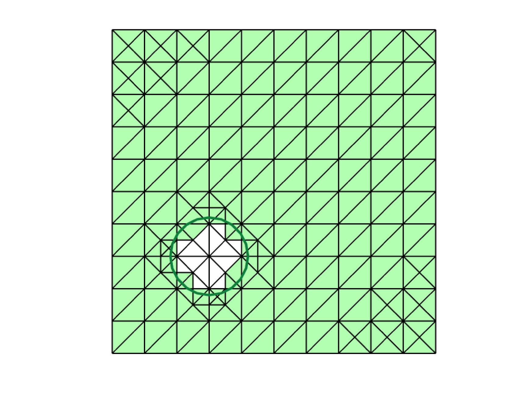
(a) Active mesh $\mathcal{A}_{h}^{s}$

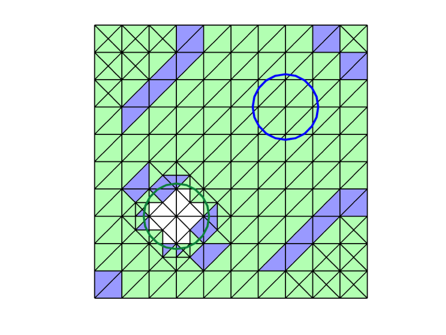
(b) Feature and elements marked for refinement (in blue)

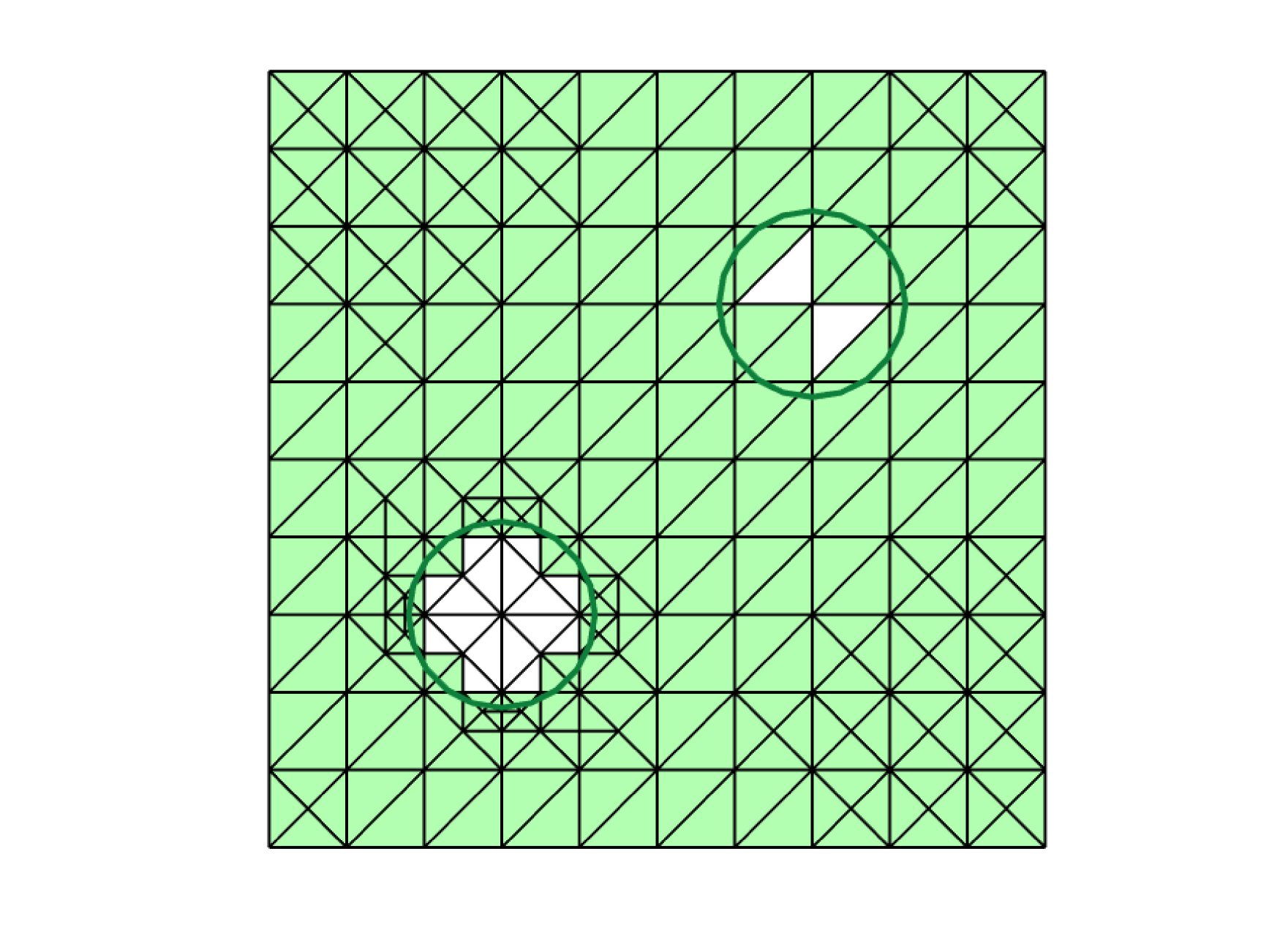
(c) Active mesh $\mathcal{A}_{h}^{s+1}$

Figure 5: Example of an iteration of combined adaptivity

Remark 6.

It is interesting to remark how, similarly to [7], the proposed adaptive strategy naturally takes care of Assumption 2. Let $F\in\tilde{\mathcal{F}}_{s}$, i.e. $F$ is a feature that is not included into the geometry at step $s$. If $F\cap K=\emptyset$ $\forall K\in\mathcal{G}_{h}^{s}$, which means that $F$ is not intersecting any element which is also intersected by a feature in $\mathcal{F}^{\star}_{s}$, then Assumption 2 is actually unnecessary for the given feature, since $||\nabla\cdot\bm{\sigma}_{h,s}-f||_{F}=0$ (see the proof of Proposition 1). However, it will still be naturally satisfied since, if the error is concentrated in the feature, this will lead to the inclusion of $F$ into the geometry. The same holds if there exists at least one element $K\in\mathcal{G}_{h}^{s}$ such that $K\cap F\neq\emptyset$. Indeed, the local contribution to the numerical component of the estimator in the elements in $\mathcal{G}_{h}^{s}$ is higher, due to the terms $\mathcal{E}_{\mathrm{div}}^{K}$ and $\mathcal{E}_{\mathrm{g}}^{K}$. This means that $K$ will be early marked for refinement, allowing to separate $F$ from the elements in $\mathcal{G}_{h}^{s}$ in a few iterations.

6 Numerical experiments

In the following we propose some numerical examples in order to validate the proposed estimator. The (weakly) equilibrated flux reconstruction is computed by solving (23) with $p=1$. Some remarks on the stabilized version (see Problem (40)) are reported for the first numerical example. For the elements $K\in\mathcal{G}_{h}^{s}$, the integrals on the active portion $K\cap\Omega_{s}^{\star}$ are computed by defining proper quadrature rules on a subtriangulation of the active portion of the element itself. The integrals on $\gamma_{\bm{a}}^{\star}$ appearing in (23) are computed by quadrature formulas on the intersection between $\mathcal{A}_{h}$ and the feature edges (see for instance [3] for a review on integration of interface terms in non-matching techniques). The same is done also in the computation of the integrals on $\tilde{\gamma}$ required in the evaluation of the defeaturing component of the estimator.

Let us remark that when no feature is included into the geometry, we have $\mathcal{E}_{K}^{2}=\mathcal{E}_{\sigma}^{2}$ for all $K\in\mathcal{A}_{h}^{s}$ and for all $s\in\mathbb{N}$. Indeed, $\mathcal{E}_{\mathrm{g}}=0$ and, since $f\in Q_{h}(\Omega_{0})$, also $\mathcal{E}_{\mathrm{div}}=0$. Hence, when in the following numerical examples we will compare the performances of the proposed adaptive procedure with standard mesh refinement, we will refer to a standard $h$-adaptivity in which the mesh is refined by the Dörfler strategy reported in Section 5.3 according only to the value of $(\mathcal{E}_{\sigma}^{K})^{2}=||\bm{\sigma}_{h}+\nabla u_{h}^{0}||^{2}_{K}$, $K\in\mathcal{T}_{h}^{s}$. We will refer to the adaptive procedure allowing both for mesh and geometric refinement as combined adaptivity. In the tests that follow, convergence trends are shown with respect to the number $N$ of degrees of freedom of $u_{h}^{\star}$. The numerical component of the estimator is approximated as $\mathcal{E}_{\mathrm{num}}=\big{(}\sum_{K\in\mathcal{A}_{h}}\mathcal{E}_{K}^{2}\big{)}^{\frac{1}{2}}$.

6.1 Test 1: single internal feature

Let $\Omega_{0}=(0,1)^{2}$ and let $F$ be a regular polygonal feature with 20 faces, having boundary $\gamma$, inscribed in a circle of radius $\varepsilon=0.04$ and centered in $(0.2,0.2)$ (see Figure 6). Let $\Omega=\Omega_{0}\setminus\overline{F}$ and let $\Gamma_{D}=\partial\Omega_{0}$. We consider the following problem:

$$\begin{cases}-\Delta u=0&\text{in }\Omega\\ u=g_{\mathrm{D}}&\text{on }\Gamma_{\mathrm{D}}\\ \nabla u\cdot\bm{n}=0&\text{on }\gamma\end{cases}$$ (60)

with

$$g_{\mathrm{D}}(x,y)=\begin{cases}e^{-8(x+y)}&\text{if }x=0\text{ or }y=0\\ 0&\text{otherwise}\end{cases}$$ (61)

The aim of this first numerical example is to analyze the convergence of the combined adaptive strategy, comparing it to the convergence of a standard one, which performs only mesh refinement. The error is computed with respect to a reference solution reported in Figure 6(a), obtained on a very fine mesh conforming to the boundary of the feature. For what concerns the total estimator $\mathcal{E}$, we choose $\alpha_{1}=\alpha_{2}=\alpha_{3}=1$. Both strategies start from the mesh reported in Figure 6(b), ($h=7.07\cdot 10^{-2}$, $N=361$ degrees of freedom for the variable $u_{h}^{\star}$), and in both cases we choose $\theta=0.3$ in (59). The adaptive strategy is stopped as $5\cdot 10^{3}$ degrees of freedom are reached for $u_{h}^{\star}$.

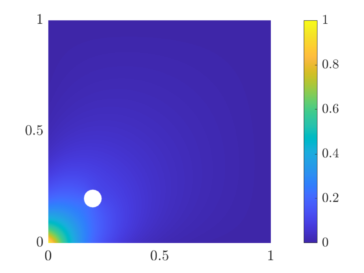
(a) Reference solution

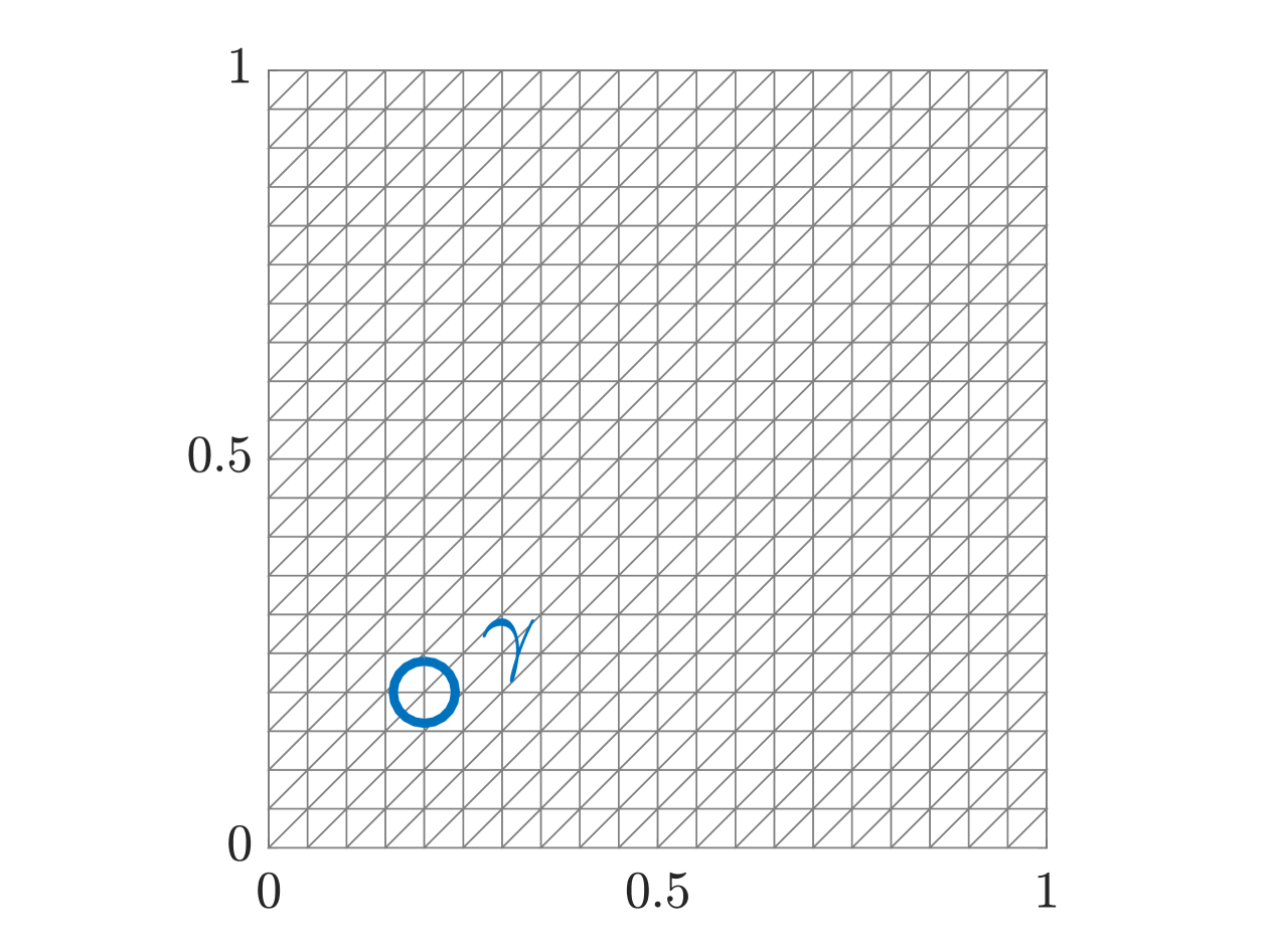
(b) Non conforming initial mesh on $\Omega_{0}$

Figure 6: Test1: reference solution and initial mesh on $\Omega_{0}$.

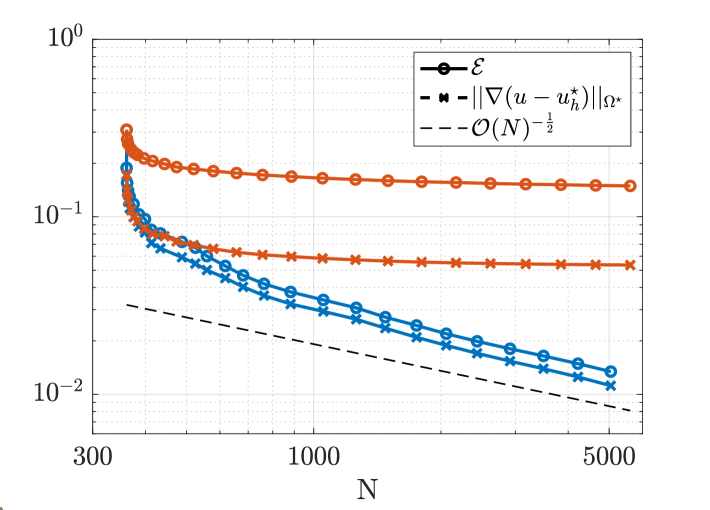
Figure 7: Test1: Convergence of the total estimator and of the overall error against the number of degrees of freedom ($N$). In blue: feature included at the first iteration; in red: feature never included.

The trend of the overall error and of the total error estimator during the adaptive procedure is reported in Figure 7. The red curves refer to the case in which the feature is not included into the geometry and only mesh refinement is performed, whereas the blue curves are obtained allowing both for mesh and geometric refinement. We can observe that, if the feature is not included, the error and the total estimator reach a plateau. On the contrary, if the feature is included into the geometry the error and the total estimator converge at the expected rate, i.e. as $\mathcal{O}(N^{-\frac{1}{2}})$, where $N$ is the total number of degrees of freedom for the variable $u_{h}^{\star}$. In particular, following the procedure devised in Section 5.3, the feature is included at the very first step, due to the predominance of the defeaturing component of the estimator on the local contributions to the numerical component. Hence, excluding the very first iteration, the whole adaptive procedure is steered by the numerical component of the estimator, as in the case in which the feature is not included. However, when the feature is included, the numerical component of the estimator accounts also for the error introduced by the weak imposition of the Neumann condition on the feature boundary. The feature is included at the very first iteration since it is located in a region in which the gradient of the solution is very steep: hence it is expected to have a strong impact on the accuracy of the solution. The step at which the feature is included could be slightly postponed by decreasing the value of $\alpha_{3}$, within the limit in which the defeaturing component of the estimator does not affect the convergence of the total estimator. As discussed in [9], the optimal value of $\alpha_{3}$ results to be problem dependent and the parameter is usually fine tuned heuristically.

The detail on the convergence of the components of the total estimator is reported in Figure 8. As expected, when the feature is not added (Figure 8(a)) the defeaturing component $\mathcal{E}_{\mathrm{def}}$ of the estimator remains almost constant, and for this reason, even if $\mathcal{E}_{\mathrm{num}}=\mathcal{E}_{\sigma}$ converges at the expected rate (as $N^{-\frac{1}{2}}$), the total estimator reaches a plateau. On the contrary, when the feature is added, $\mathcal{E}_{\mathrm{def}}=0$ starting from the second iteration (Figure 8(b)) and the total estimator converges as $N^{-\frac{1}{2}}$.

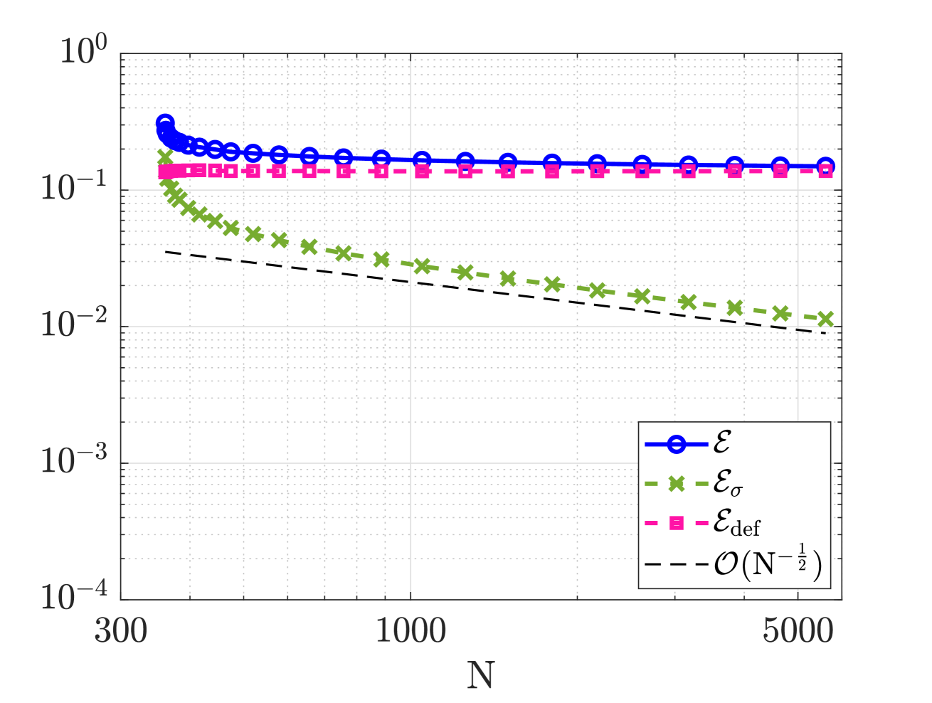
(a) No feature is included

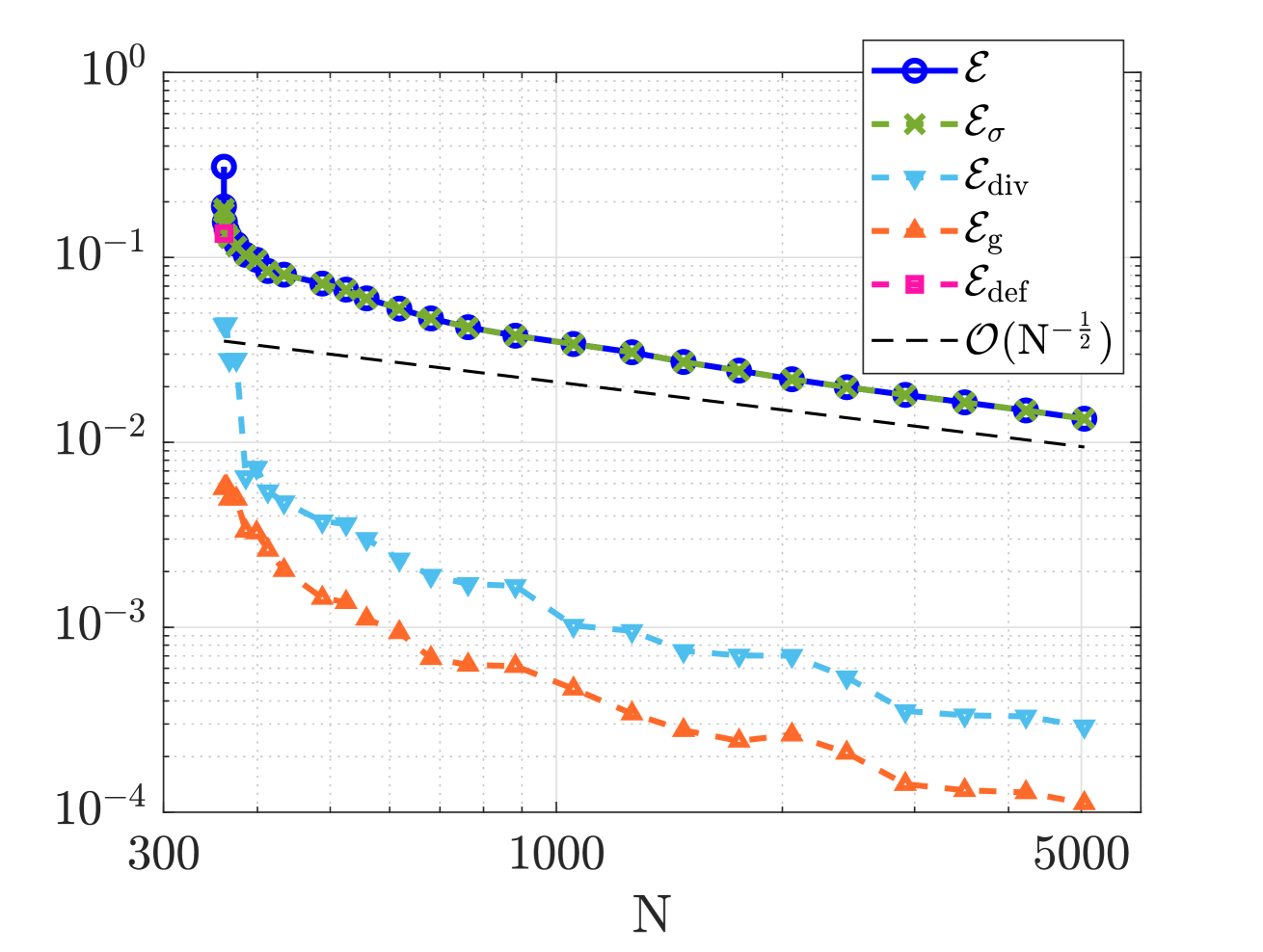
(b) Feature included at iteration 1

Figure 8: Test1: Convergence of the total estimator and of its components with respect to the number of degrees of freedom ($N$).

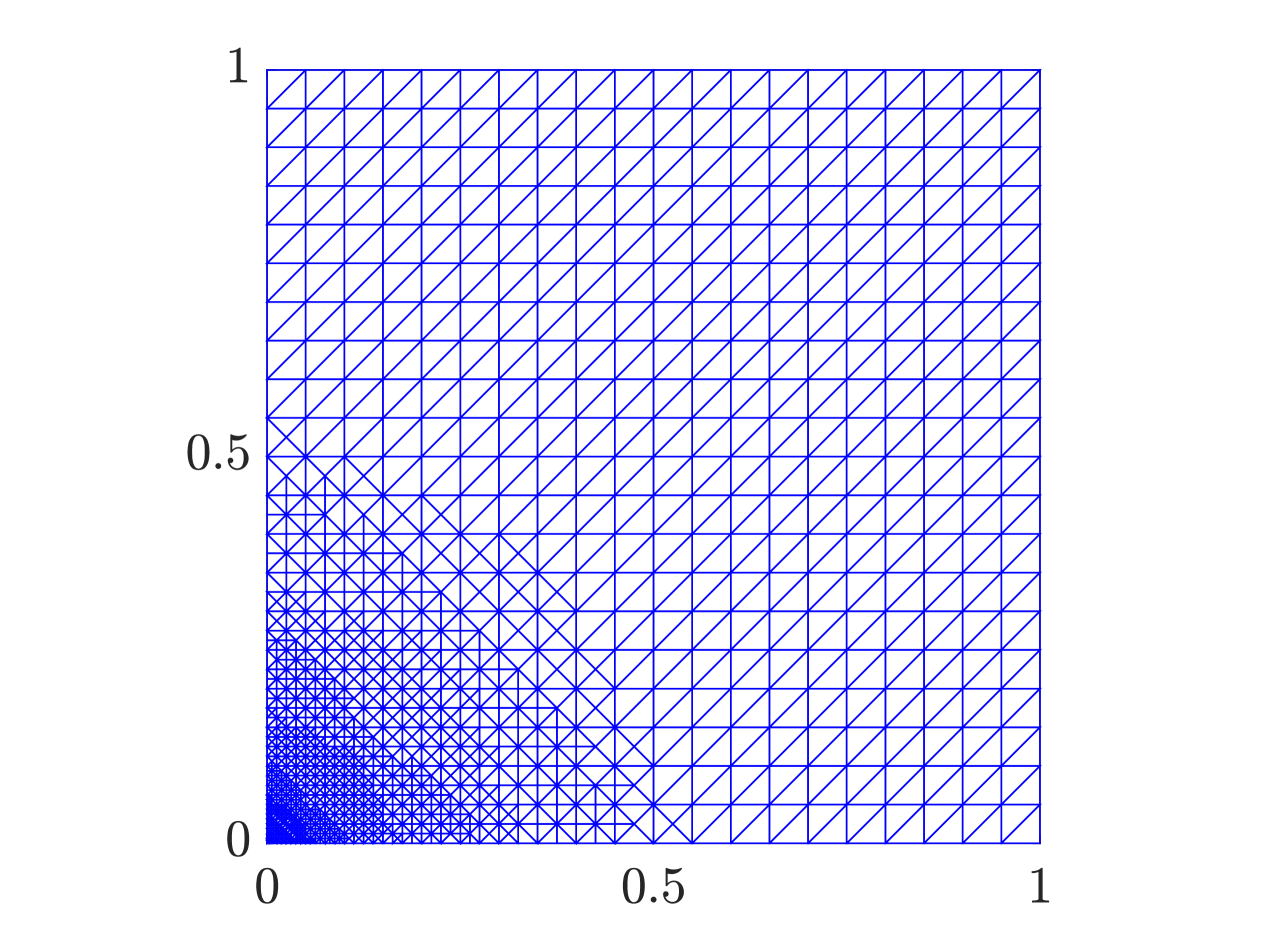
(a) No feature is included

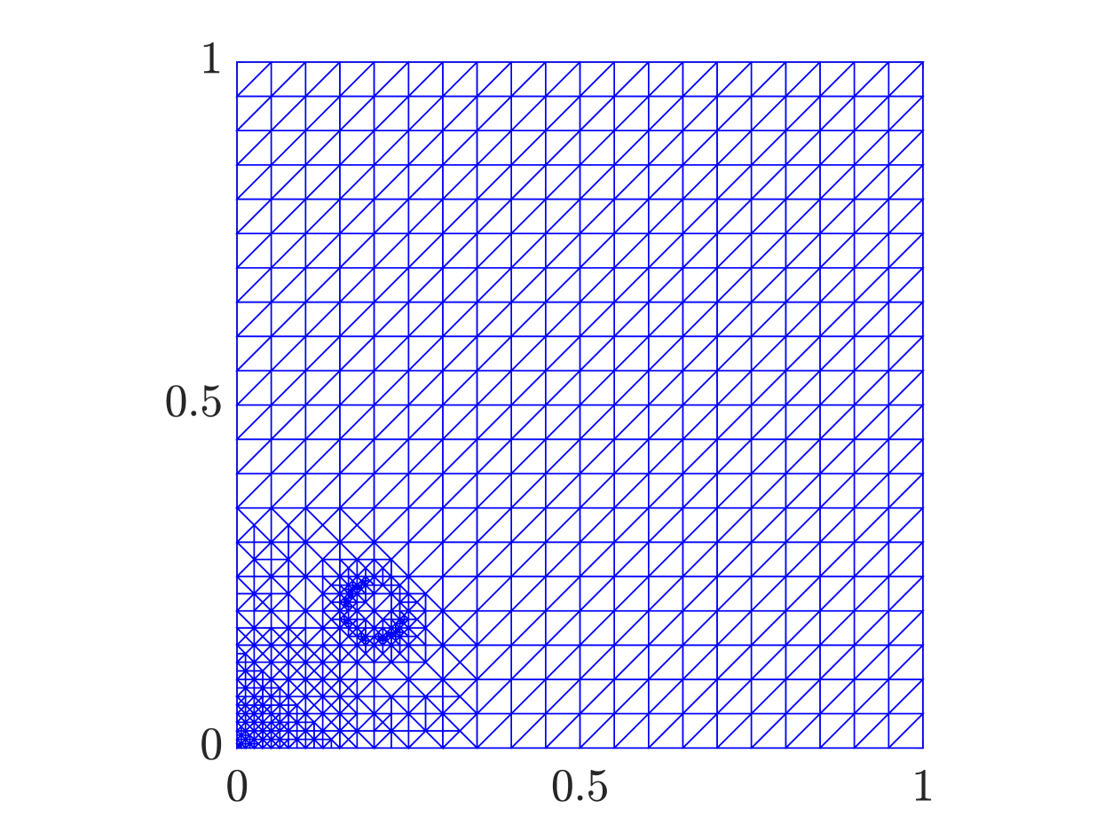
(b) Feature is included at iteration 1

Figure 9: Test 1: Adapted mesh after 15 steps of the adaptive procedure.

The meshes obtained after 15 steps of the adaptive procedure are reported in Figure 9, both for standard mesh adaptivity and for combined adaptivity. As expected, in both cases the mesh appears to be refined towards the bottom left corner of the domain. However, we can observe how the combination of mesh and geometric refinement allows the mesh to capture the feature boundary.

As reported in Remark 2, the weak imposition of Neumann boundary conditions in the computation of the weakly equilibrated flux reconstruction $\bm{\sigma}_{h}$ may require stabilization in presence of very small cuts. Figure 10(b) reports the detail on the convergence of the components of the estimator when the stabilized problem (40) is solved instead of (23). The curves obtained in the case with no stabilization, which were reported in Figure 8, are re-proposed and rescaled in Figure 10(a) to ease the comparison. As expected, the main drawback of activating the stabilization terms (38)-(39) is represented by an increase of $\mathcal{E}_{\mathrm{div}}$, which is due to the fact that mass conservation is further deteriorated with respect to the non-stabilized case, involving all the cut patches. However, this local increase of $\mathcal{E}_{\mathrm{div}}^{K}$ produces a stronger mesh refinement close to the feature, which ends up in a faster decrease of $\mathcal{E}_{\mathrm{g}}$. For this reason, the final impact of stabilization on the total estimator is pretty low, and by decreasing the value of $\alpha_{1}$ the effectivity index of the non stabilized case could be restored. Let us remark that in this case, in which the feature is added at the very first iteration, the inclusion of stabilizing terms does not deteriorate the convergence rate of the total estimator. In a different scenario, characterized by the presence of multiple features which are added at different stages of the adaptive procedure, the parameters $\alpha_{1},\alpha_{2},\alpha_{3}$ and $\beta_{1},\beta_{2}$ would need to be properly tuned, which is not always trivial. For this reason, from a barely practical standpoint, the easiest way to avoid the issues related to small cuts, may be to neglect badly cut patches, which have a small impact on the reconstructed flux. Let us recall, indeed, that the reconstructed flux is needed only to evaluate the estimator, and is not the primal variable of the problem.

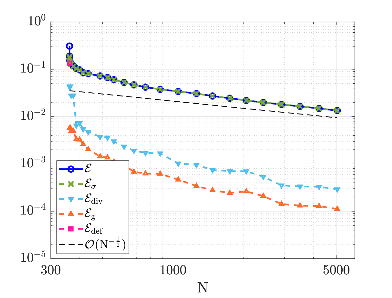
(a) No stabilization

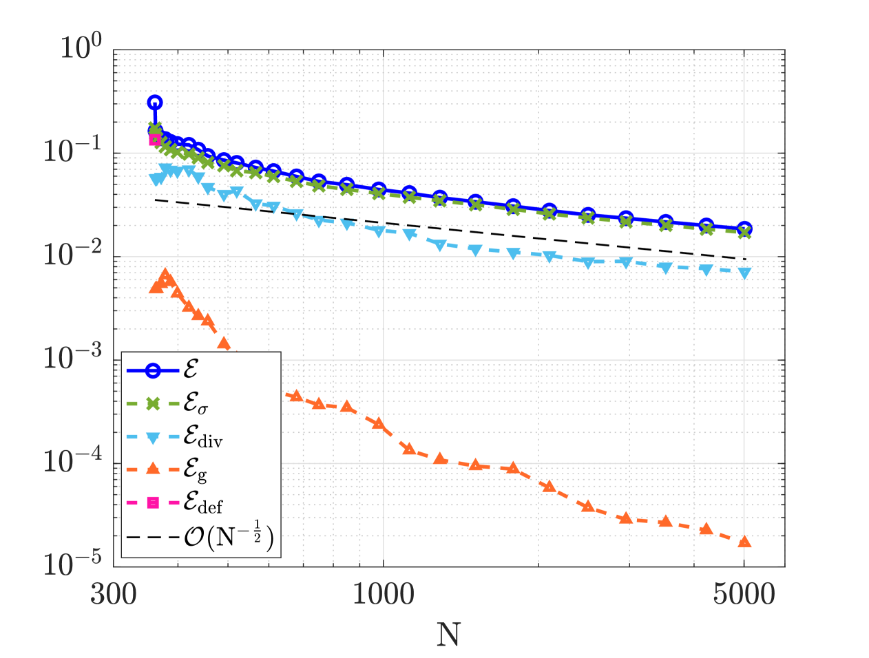
(b) With stabilization

Figure 10: Test 1: Convergence with respect to the number of degrees of freedom (N) of the total estimator and of its components with and without stabilization

6.2 Test 2: multiple internal and boundary features

The aim of this second numerical experiment is to test the proposed adaptive procedure on a case characterized by the presence of multiple features, both internal and on the boundary. Let again $\Omega_{0}=(0,1)^{2}$ and let us consider a set $\mathcal{F}=\{F_{i}\}_{i=1}^{37}$ of 37 features, being all regular polygons inscribed in a circle of radius $\epsilon_{i}$, centered in $\bm{x}_{i}^{C}$, having $n_{i}^{e}$ edges and rotated of an angle $\theta_{i}$ with respect to a reference orientation in which one of the vertexes is located in $\bm{x}_{i}^{C}+[0,\epsilon_{i}]$. In particular, denoting by $\mathcal{U}(a,b)$ a standard uniform distribution between $a$ and $b$, we take $\epsilon_{i}\sim\mathcal{U}(1e-3,5e-2)$ and $\theta_{i}\sim\mathcal{U}(0,2\pi)$. For internal features $\bm{x}_{i}^{C}\sim\mathcal{U}(0.1,0.9)^{2}$, while for boundary features $\bm{x}_{i}^{C}\sim\{0,1\}\times\mathcal{U}(0.1,0.9)$. For both cases the number of edges $n_{i}^{e}$ is chosen from a discrete integer uniform distribution between 4 and 16. The actual data used in the experiments are available in the Appendix.

On $\Omega=\Omega_{0}\setminus\{\overline{F},~F\in\mathcal{F}\}$ we consider the following test problem:

$$\begin{cases}-\Delta u=0&\text{in }\Omega\\ u=g_{\mathrm{D}}&\text{on }\Gamma_{\mathrm{D}}\\ \nabla u\cdot\bm{n}=0&\text{on }\Gamma_{\mathrm{N}}\end{cases}$$ (62)

with $\Gamma_{\mathrm{D}}=\{(x,y):y\in\{0,1\}\}$ and

$$g_{\mathrm{D}}(x,y)=\begin{cases}e^{-8(x+y)}&\text{if }y=0\\ 0&\text{if }y=1.\end{cases}$$ (63)

The behavior of $u$ is very similar to the one in Test 1; however the presence of Neumann boundaries allows us to set some features along the boundary itself. For what concerns the (partially) defeatured problem, we choose $g_{0}=0$ (see (5) and (13)).

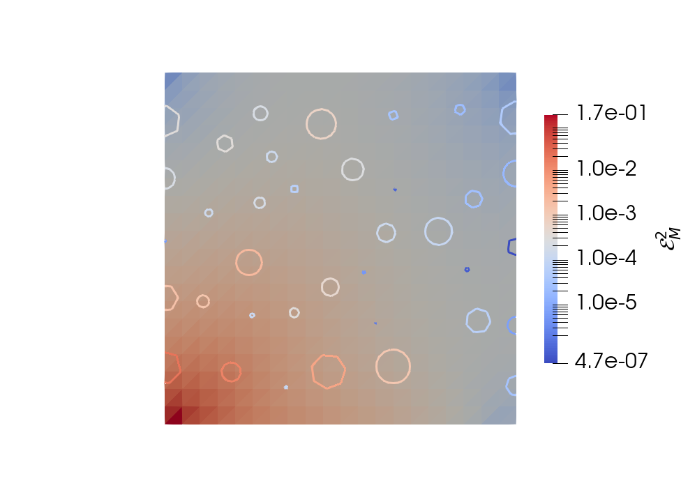
Figure 11: Test 2: Square of the local numerical components and of the local defeaturing components of the estimator at the first iteration of the adaptive procedure.

The features in $\mathcal{F}$ are shown in Figure 11, which also reports the initial values of the square of the local contributions to the numerical and the defeaturing component of the estimators, i.e. the values contained in $\mathcal{E}_{M}^{2}$ at the very first application of the Dörfler strategy reported in Section 5.3. The initial mesh $\mathcal{T}_{h}^{0}$ is the same used in Test 1 ($h=7.07\cdot 10^{-2}$), ending however up in $N=399$ degrees of freedom for the variable $u_{h}^{\star}$, due to the different choice of the boundary conditions.

Figure 12 compares the convergence of the error estimator and of its components in two scenarios: the blue curves refer to the case in which the adaptive strategy proposed in Section 5 is applied with $\alpha_{1}=\alpha_{2}=\alpha_{3}=1$, whereas the red curves are obtained without including any feature, i.e. with standard mesh refinement based on the value of $(\mathcal{E}_{\sigma}^{K})^{2}$. As in the previous numerical test, we can observe how, in this second case, the total estimator rapidly reaches a plateau, due to the fact that the defeaturing component of the estimator remains constant. Allowing instead for both mesh and geometric refinement the total estimator tends to converge as $N^{-\frac{1}{2}}$, i.e. as the numerical component. Figure 13 shows the computational mesh after 6 iterations of the adaptive procedure, both for standard mesh adaptivity and for the combined one. At this stage, if no features are included, the total estimator is reduced of about $27\%$ with respect to its initial value while, if we allow also for geometric adaptivity, $\mathcal{E}$ is reduced of about $50\%$, with only 7 features included. As expected, and as shown in Figure 13(b), these 7 features are the biggest among the ones closest to the bottom left corner, which is coherent also with the results in [7]. The adaptive process is stopped as $5\cdot 10^{3}$ degrees of freedom are reached. At this stage, in the combined strategy, all the features are included (all the features are actually included before iteration 26) and the total estimator has been reduced of about $94\%$, against a relative decrease of $47\%$ in the standard mesh adaptivity case. Figure 14 shows the final meshes, both for standard and combined adaptivity.

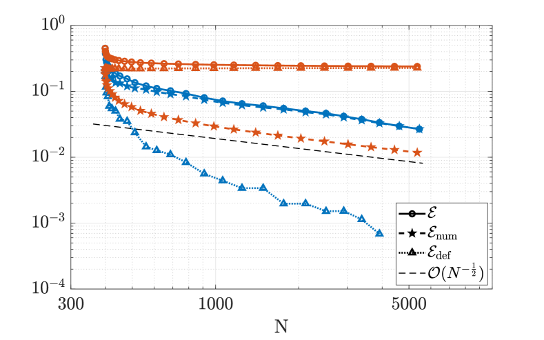
Figure 12: Test 2: Convergence of the total estimator and of its components at the increase of the number of degrees of freedom (N). In red, no feature included; in blue features included with $\alpha_{3}=1$.

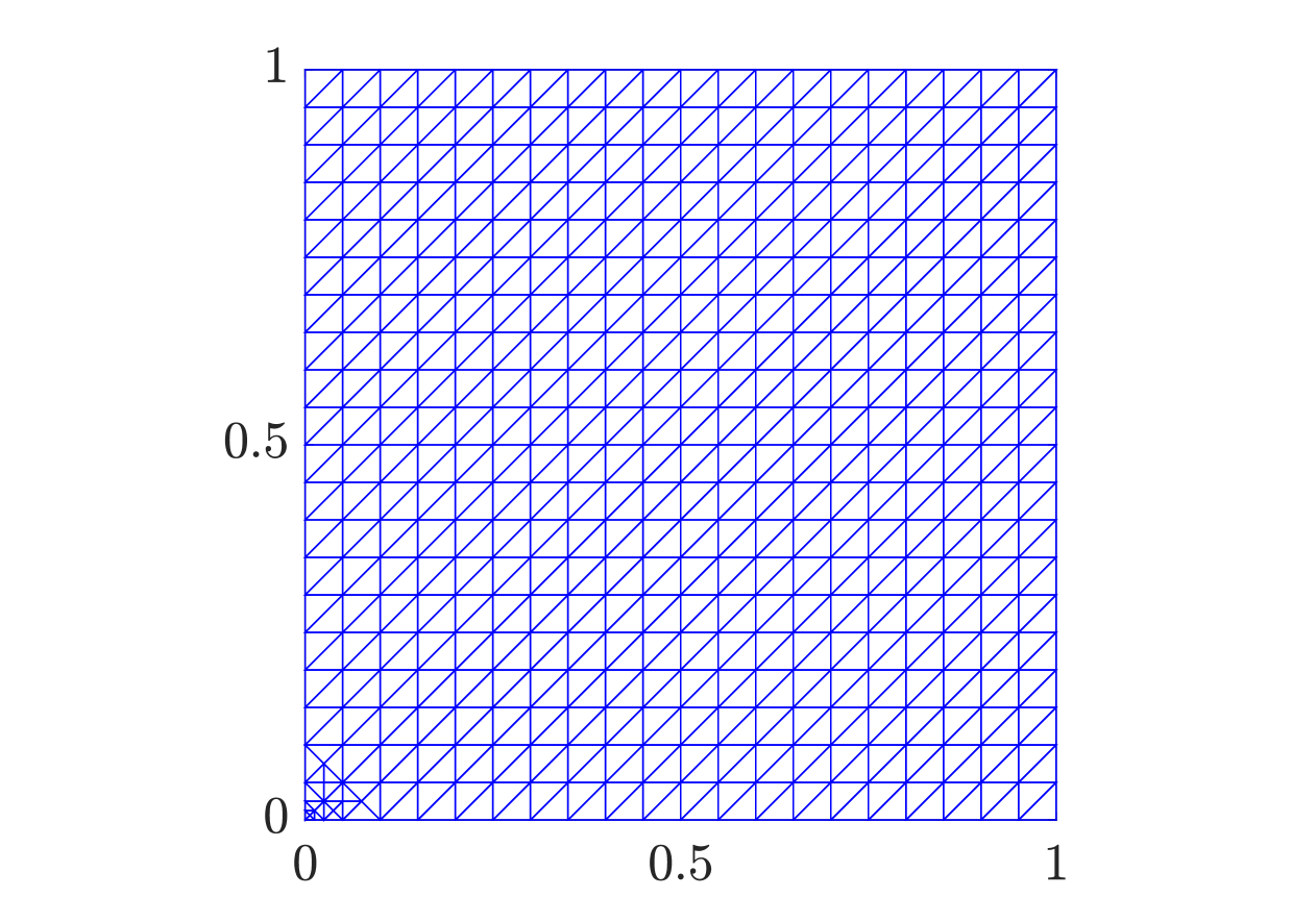
(a) Mesh adaptivity

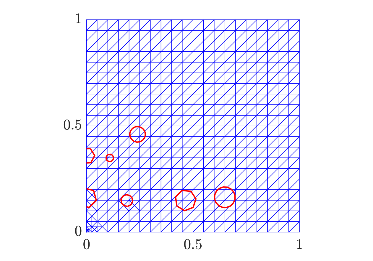
(b) Combined adaptivity

Figure 13: Test 2: Adapted mesh after 6 iterations of the adaptive procedure (included features highlighted for the geometric adaptivity case).

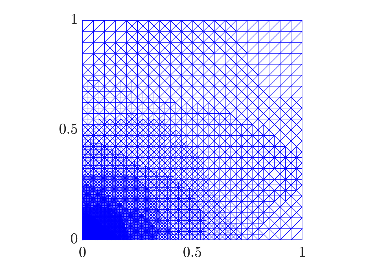
(a) Mesh adaptivity

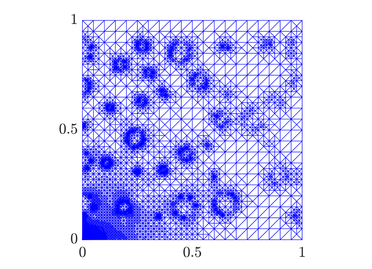
(b) Combined adaptivity

Figure 14: Test 2: Adapted mesh after 27 iterations of the adaptive procedure.

6.3 Test 3: multiple internal features, discontinuous coefficient

For this last numerical example let us choose $\Omega_{0}=(-1,1)^{2}$ and let $\mathcal{F}$ be a set of 19 negative, internal, polygonal features (see Figure 15(a)), divided into two sets: $\mathcal{F}_{\mathrm{rand}}=\{{F_{i}}\}_{i\in\mathcal{I}_{\mathrm{rand}}}$ and $\mathcal{F}_{\mathrm{sing}}=\{{F_{i}}\}_{i\in\mathcal{I}_{\mathrm{sing}}}$. The 10 features in $\mathcal{F}_{\mathrm{rand}}$ are randomly built as in Test 2, with $\epsilon_{i}\sim\mathcal{U}(2e-3,1e-1)$, and $\bm{x}_{i}^{C}\sim\mathcal{U}(-0.9,0.9)^{2}$, $i\in\mathcal{I}_{\mathrm{rand}}$. The position of the 9 features in $\mathcal{F}_{\mathrm{sing}}$ is instead given, in particular, for $\forall i\in\mathcal{I}_{\mathrm{sing}}$, $\bm{x}_{j}^{C}\in\{-\frac{1}{2},0,\frac{1}{2}\}\times\{-\frac{1}{2},0,\frac{1}{2}\}$, while $\epsilon_{i}\sim\mathcal{U}(6e-2,1e-1)$. For both set of features, i.e. for $i\in\mathcal{I}_{\mathrm{rand}}\cup\mathcal{I}_{\mathrm{sing}}$, $\theta_{i}\sim\mathcal{U}(0,2\pi)$, while the number of edges $n_{i}^{e}$ is chosen from a discrete uniform distribution between 4 and 16, as in Test 2. The specific feature data that were chosen for the proposed numerical experiment are reported in the Appendix.

On $\Omega=\Omega_{0}\setminus\{\overline{F},~F\in\mathcal{F}\}$ we consider the following problem:

$$\begin{cases}-\nabla\cdot(\kappa\nabla u)=0&\text{in }\Omega\\ u=g_{\mathrm{D}}&\text{on }\Gamma_{\mathrm{D}}\\ \nabla u\cdot\bm{n}=0&\text{on }\Gamma_{\mathrm{N}}\end{cases}$$ (64)

with $\kappa$ being a discontinuous piecewise constant coefficient taking values $1$ and $100$ in a $4\times 4$ chessboard pattern, as reported in Figure 15(b). The features in $\mathcal{F}_{\mathrm{sing}}$ are hence exactly centered in the singularities produced by this piecewise constant coefficient.

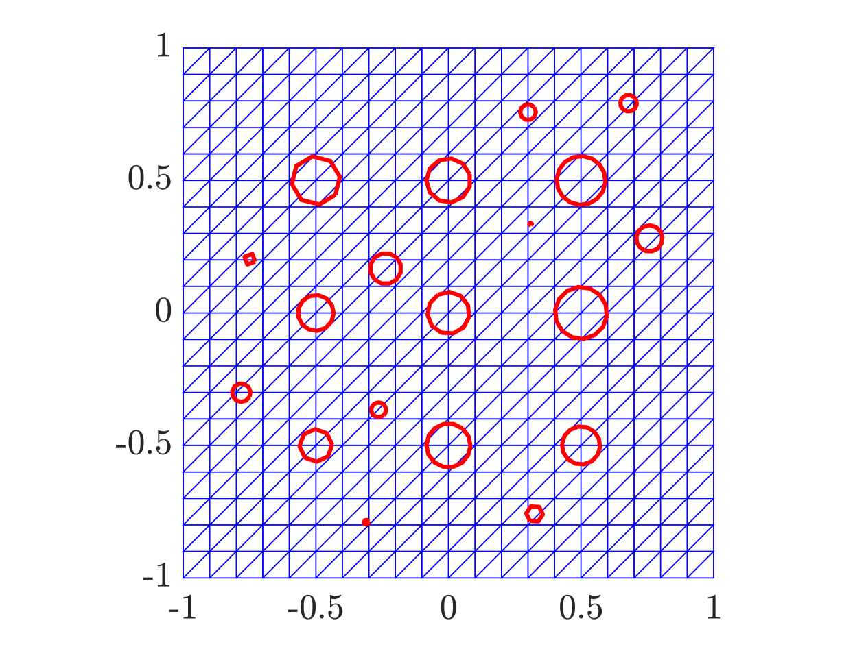
(a) Features and initial mesh

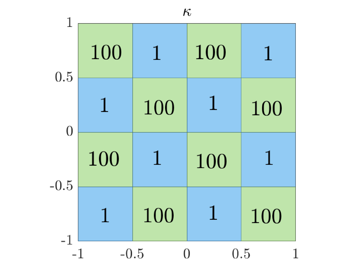
(b) Diffusion coefficient $\kappa$

Figure 15: Test 3: initial mesh, features and chessboard diffusion coefficient

The Dirichlet datum is chosen as a piecewise linear function. In particular, introducing

$$\mu_{1}(t)=\begin{cases}2&\text{if }t\in[-1,-\frac{1}{2})\\ -t+\frac{3}{2}&\text{if }t\in[-\frac{1}{2},0)\\ \frac{3}{2}&\text{if }t\in[0,\frac{1}{2})\\ -t+2&\text{if }t\in[\frac{1}{2},1],\end{cases}\quad\mu_{2}(t)=\begin{cases}-t&\text{if }t\in[-1,-\frac{1}{2})\\ \frac{1}{2}&\text{if }t\in[-\frac{1}{2},0)\\ -t+\frac{1}{2}&\text{if }t\in[0,\frac{1}{2})\\ 0&\text{if }t\in[\frac{1}{2},1],\end{cases}$$

we define

$$g_{\mathrm{D}}(x,y)=\begin{cases}\mu_{2}(x)&\text{if }y=-1\\ \mu_{1}(-y)&\text{if }x=-1\\ \mu_{1}(x)&\text{if }y=1\\ \mu_{2}(-y)&\text{if }x=1.\end{cases}$$

The initial mesh $\mathcal{T}_{h}^{0}$, which conforms the jumps in the coefficient $\kappa$, is reported in Figure 15(a). It is obtained by setting $h=1.41\cdot 10^{-1}$, ending up with $N=361$ degrees of freedom for variable $u_{h}^{\star}$

Remark 7.

Despite having introduced a coefficient $\kappa\neq 1$, we still compute the (weakly) equilibrated flux reconstruction as a discrete approximation of $\bm{\sigma}\in\bm{H}(\text{div},\Omega^{\star})$ satisfying (17). For this reason we have to slightly modify the definition of the estimator, by setting $(\mathcal{E}_{\sigma}^{K})^{2}=||\bm{\sigma}_{h}+\kappa\nabla u_{h}^{\star}||_{K\cap{\Omega^{\star}}}^{2}$, whereas the other components remain unchanged. The (weakly) equilibrated flux reconstruction is still computed by summing the solutions of patch-local problems in the form of (23). The non-unitary coefficient $\kappa$ affects only the right hand side of the system, whose components need to be redefined as

$$L_{\bm{a}}(\bm{v_{h}}):=-(\psi_{\bm{a}}(\kappa\nabla u_{h}^{\star}),\bm{v}_{h})_{{\omega}_{\bm{a}}^{\star}}-\frac{1}{h_{\bm{a}}}\langle\psi_{\bm{a}}g,\bm{v}_{h}\cdot\bm{n}\rangle_{\gamma_{\bm{a}}^{\star}}$$

$$R_{\bm{a}}^{p}(q_{h})=(\psi_{\bm{a}}f-\nabla\psi_{\bm{a}}\cdot(\kappa\nabla u_{h}^{\star}),q_{h})_{{\omega}_{\bm{a}}^{\star}}+p\langle\psi_{\bm{a}}g,q_{h}\rangle_{\gamma_{\bm{a}}^{\star}},$$

Figure 16 reports the trend of the total error estimator and of its components during the adaptive process, considering both standard $h$-adaptivity and combined adaptivity. In both cases we choose $\theta=0.5$ in the Dörfler marking strategy (59) and we stop before 6000 degrees of freedom are reached. The parameters $\alpha_{1},\alpha_{2},\alpha_{3}$ are all set equal to 1.

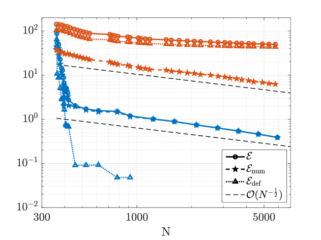
Figure 16: Test 3: Convergence of the total estimator and of its components at the increase of the number of degrees of freedom. In red, no feature included; in blue, features included with $\alpha_{3}=1$.

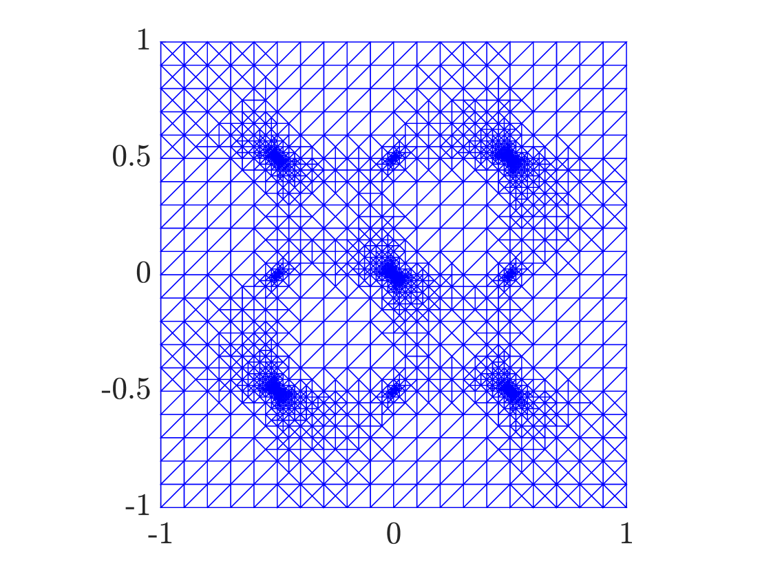
(a) Final mesh

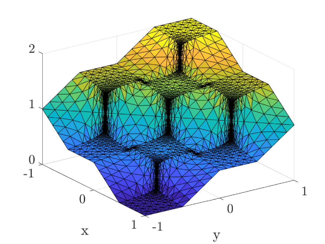
(b) Final numerical solution

Figure 17: Test 3: Final mesh and numerical solution in the case of standard mesh adaptivity (no feature is included).

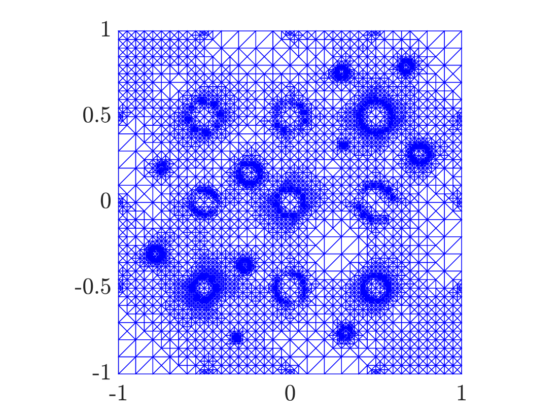
(a) Final mesh

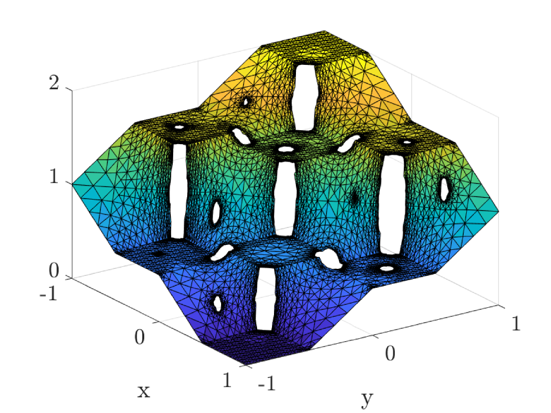
(b) Final numerical solution

Figure 18: Test 3: Final mesh and numerical solution in the case of combined adaptivity.

In the case of $h$-adaptivity we can observe how the total estimator converges very slowly, steered by the defeaturing component, which remains almost constant. The slight decrease of $\mathcal{E}_{\mathrm{def}}$, in particular in the first iterations, is related to the fact that the solution on the features centered in the singularities undergoes quick changes during the first refinement steps. The final mesh is reported in Figure 17(a), while the final numerical solution is shown in Figure 17(b). In the case of the combined adaptivity we can instead observe how the total estimator tends to converge at the expected rate, completely steered by the numerical component, to which it is almost perfectly overlapped. The sudden decrease of the estimator in the first part of the adaptation is related to the fact that all the features in $\mathcal{F}_{\mathrm{sing}}$ are marked for inclusion during the first iterations. After that, in a few steps in which the mesh is refined close to these features, the singularities are finally excluded from the active mesh. The features in $\mathcal{F}_{\mathrm{rand}}$ are instead added a bit later, but all within iteration 22. The final mesh, along with the corresponding numerical solution is reported in Figure 18(a).

Let us remark that, even if they are included later, the features in $\mathcal{F}_{\mathrm{rand}}$ are actually relevant for the accuracy of the solution. This is shown in Figure 19, which reports the trend of the total estimator in a case in which the features in $\mathcal{F}_{\mathrm{rand}}$ are artificially not marked for inclusion although the estimator suggests to include them. Despite the rapid decrease related to the inclusion of the other features, $\mathcal{E}$ tends to stagnate, not reaching the expected convergence rate. Figure 19 shows the trend of the estimator also in a case in which only the features in $\mathcal{F}_{\mathrm{rand}}$ are marked for inclusion, showing how, if the singularities are not excluded, there is almost no difference with the case in which the features are not added at all. This confirms the capability of the estimator, of course when the features are not artificially unmarked, to include the features in the most suitable order.

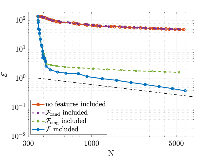
Figure 19: Test 3: Convergence with respect to the number of degrees of freedom (N) of the total estimator for different sets of features considered for inclusion.

7 Conclusions

An adaptive strategy based on an equilibrated flux a posteriori error estimator was proposed for defeaturing problems, extending the work in [6] to the case of trimmed geometries. The focus is kept on Poisson’s problem with Neumann boundary conditions on the feature boundary and, in particular, on the negative feature case. Similarly to [7] the adaptive strategy accounts both for standard mesh refinement and geometric refinement, i.e. for feature inclusion. The resulting adaptive strategy is called combined adaptivity.

In order to never remesh the considered domain, the features are progressively included into the geometry using a CutFEM strategy, and an equilibrated flux reconstruction is computed by imposing weakly, through Nitsche’s method, the Neumann boundary conditions on the feature boundaries. Hence the estimator also accounts for the error committed in the imposition of such boundary conditions and for the consequent mass unbalance.

The use of a reconstructed flux allows us to never evaluate the numerical flux on the boundary of the features, which is a great advantage for finite element discretizations, in which the gradient of the numerical solution is typically discontinuous across element edges. Furthermore, until no features are included into the geometry, it allows us to sharply bound the numerical component of the error, hence reducing the number of parameters to be fine tuned for the application of the adaptive procedure.

The reliability of the estimator was proven in $\mathbb{R}^{d}$, $d=2,3$ and verified on three different numerical examples in $\mathbb{R}^{2}$, also involving multiple features of different sizes, both internal and on the boundary. The generalization to the positive feature case is left to a forthcoming work, as well as the validation of the proposed adaptive strategy on three-dimensional geometries, this second having an impact mainly on computational aspects.

Appendix A Appendix

In this appendix we provide the data of the features that were used for Test 2 and Test 3. A generic feature $F_{i}$ is assumed to be a polygon inscribed in a circle of radius $\epsilon_{i}$, centered in $\bm{x}_{i}^{C}=(x_{i}^{C},y_{i}^{C})$, having $n_{i}^{e}$ edges and rotated of an angle $\theta_{i}$ with respect to a reference orientation in which one of the vertexes is located in $\bm{x}_{i}^{C}+[0,\epsilon_{i}]$.

Table 1: Feature data for Test 2

$\bm{i}$	$\epsilon_{i}$	$x_{i}^{C}$	$y_{i}^{C}$	$n_{i}^{e}$	$\theta_{i}$	$\bm{i}$	$\epsilon_{i}$	$x_{i}^{C}$	$y_{i}^{C}$	$n_{i}^{e}$	$\theta_{i}$
1	0.0128	0.3695	0.6692	4	224.9859	20	0.0156	0.8396	0.8958	5	154.4009
2	0.0239	0.1714	0.7986	6	24.2550	21	0.0057	0.8600	0.4401	8	134.2678
3	0.0314	0.5347	0.7247	11	29.1858	22	0.0367	0.2399	0.4603	16	73.3359
4	0.0277	0.1893	0.1487	10	190.0490	23	0.0045	0.5668	0.4321	4	68.2234
5	0.0352	0.8916	0.2945	7	262.3478	24	0.0158	0.3045	0.7608	7	52.4692
6	0.0487	0.6498	0.1642	16	125.5876	25	0.0202	0.2724	0.8842	15	19.4049
7	0.0269	0.6300	0.5445	8	87.1778	26	0.0388	0.7788	0.5486	14	108.5075
8	0.0174	0.1094	0.3495	13	56.1573	27	0.0023	0.5995	0.2871	4	185.3529
9	0.0110	0.1255	0.6014	8	126.4299	28	0.0302	0.0000	0.6995	11	6.0078
10	0.0156	0.2704	0.6302	11	81.7039	29	0.0386	0.0000	0.3592	6	357.7583
11	0.0422	0.4453	0.8543	16	184.2681	30	0.0452	0.0000	0.8618	6	336.7216
12	0.0058	0.2489	0.3096	11	124.2501	31	0.0475	0.0000	0.1621	6	75.1260
13	0.0148	0.6500	0.8789	4	115.4929	32	0.0036	0.0000	0.5210	9	238.0898
14	0.0254	0.4708	0.3901	9	281.4964	33	0.0484	1.0000	0.8710	7	265.5165
15	0.0138	0.3684	0.3172	8	346.0244	34	0.0249	1.0000	0.2814	16	233.4964
16	0.0492	0.4653	0.1502	7	249.4054	35	0.0295	1.0000	0.1099	7	275.1374
17	0.0045	0.3452	0.1051	5	17.9789	36	0.0273	1.0000	0.5045	5	147.7730
18	0.0026	0.6548	0.6676	10	66.5531	37	0.0376	1.0000	0.7132	13	176.2045
19	0.0247	0.8788	0.6407	7	48.8767

Table 2: Feature data for Test 3

$\bm{i}$	$\epsilon_{i}$	$x_{i}^{C}$	$y_{i}^{C}$	$n_{i}^{e}$	$\theta_{i}$	$\bm{i}$	$\epsilon_{i}$	$x_{i}^{C}$	$y_{i}^{C}$	$n_{i}^{e}$	$\theta_{i}$
1	0.0617	-0.5000	-0.5000	8	87.1778	11	0.0219	-0.7489	0.2029	4	115.4929
2	0.0674	-0.5000	0.0000	13	56.1573	12	0.0297	0.3001	0.7578	10	70.8553
3	0.0915	-0.5000	0.5000	8	126.4299	13	0.0276	-0.2632	-0.3656	16	137.5424
4	0.0830	0.0000	-0.5000	14	26.4852	14	0.0090	-0.3096	-0.7899	7	85.2644
5	0.0791	0.0000	0.0000	11	338.4382	15	0.0051	0.3097	0.3352	4	165.5202
6	0.0833	0.0000	0.5000	11	81.7039	16	0.0495	0.7576	0.2813	13	327.8332
7	0.0719	0.5000	-0.5000	14	261.8490	17	0.0313	0.6791	0.7915	12	39.8837
8	0.0981	0.5000	0.0000	14	212.4525	18	0.0315	0.3245	-0.7584	6	243.2179
9	0.0921	0.5000	0.5000	16	184.2681	19	0.0585	-0.2369	0.1675	12	225.4836
10	0.0347	-0.7811	-0.3010	11	124.2501

References

- [1] M. Ainsworth and J.T. Oden “A posteriori error estimation in finite element analysis” In Computer Methods in Applied Mechanics and Engineering 142.1, 1997, pp. 1–88
- [2] P. Antolťın and O. Chanon “Analysis-aware defeaturing of complex geometries with Neumann features” In Int. J. Numer. Methods Eng., 2023
- [3] D. Boffi et al. “A comparison of non-matching techniques for the finite element approximation of interface problems” In Computers and Mathematics with Applications 151, 2023, pp. 101–115 DOI: https://doi.org/10.1016/j.camwa.2023.09.017
- [4] D. Braess “Finite elements - Theory, fast solvers, and applications in solid Mechanics”, 2007
- [5] D. Braess and J. Schöberl “Equilibrated Residual Error Estimator for Edge Elements” In Mathematics of Computation 77.262 American Mathematical Society, 2008, pp. 651–672
- [6] A. Buffa et al. “An equilibrated flux a posteriori error estimator for defeaturing problems” In SIAM Journal on Numerical Analysis 62.6, 2024, pp. 2439–2458 DOI: 10.1137/23M1627195
- [7] A. Buffa, O. Chanon and R. Vázquez “Adaptive analysis-aware defeaturing: the case of Neumann boundary conditions” arXiv:2212.05183, 2022
- [8] A. Buffa, O. Chanon and R. Vázquez “An a posteriori error estimator for isogeometric analysis on trimmed geometries” In IMA Journal of Numerical Analysis 43, 2023, pp. 2533–2561
- [9] A. Buffa, O. Chanon and R. Vázquez “Analysis-aware defeaturing: Problem setting and a posteriori estimation.” In Math. Models Methods Appl. Sci. 32.2, 2022, pp. 359–402
- [10] E. Burman “Ghost penalty” In Comptes Rendus Mathematique 348.21, 2010, pp. 1217–1220 DOI: 10.1016/j.crma.2010.10.006
- [11] E. Burman, S. Claus P. Hansbo, M.G. Larsson and A. Massing “CutFEM: Discretizing geometry and partial differential equations” In International Journal for Numerical Methods in Engineering 104.7, 2015, pp. 472–501 DOI: https://doi.org/10.1002/nme.4823
- [12] K. K. Choi and N.-H. Kim “Structural Sensitivity Analysis and Optimization 1: Linear Systems” In Springer Science and Business Media, 2005
- [13] D. Capatina, and C. He “Flux recovery for Cut Finite Element Method and its application in a posteriori error estimation” In ESAIM: M2AN 55.6, 2021, pp. 2759–2784 DOI: 10.1051/m2an/2021071
- [14] P. Destuynder and B. Métivet “Explicit Error Bounds in a Conforming Finite Element Method” In Mathematics of Computation 68.228, 1999, pp. 1379–1396
- [15] A. Ern and M. Vohralík “Polynomial-degree-robust a posteriori estimates in a unified setting for conforming, nonconforming, discontinuous Galerkin, and mixed discretizations” In SIAM Journal on Numerical Analysis 53.2, 2015, pp. 1058–1081
- [16] R. Ferrandes, P. Marin, J.-C. Léon and F. Giannini “A posteriori evaluation of simplification details for finite element model preparation” In Computers and Structures 87.1, 2009, pp. 73–80
- [17] L. Fine, L. Remondini and J.-C. Leon “Automated generation of FEA models through idealization operators” In International Journal for Numerical Methods in Engineering 49.1-2, 2000, pp. 83–108
- [18] G. Foucault, P. M. Marin and J.-C Léon “Mechanical Criteria for the Preparation of Finite Element Models” In International Meshing Roundtable Conference, 2004
- [19] T. Frachon, P. Hansbo, E. Nilsson and S. Zahedi “A Divergence Preserving Cut Finite Element Method for Darcy Flow” In SIAM Journal on Scientific Computing 46.3, 2024, pp. A1793–A1820 DOI: 10.1137/22M149702X
- [20] S. H. Gopalakrishnan and K. Suresh “A formal theory for estimating defeaturing-induced engineering analysis errors” In Computer-Aided Design 39.1, 2007, pp. 60–68
- [21] S. H. Gopalakrishnan and K. Suresh “Feature sensitivity: a generalization of topological sensitivity” In Finite Elements in Analysis and Design 44.11, 2008, pp. 696–704
- [22] A. Hansbo and P. Hansbo “An unfitted finite element method, based on Nitsche’s method, for elliptic interface problems” In Comput. Methods Appl. Mech. Eng. 191, 2002, pp. 5537–5552
- [23] M. Li and S. Gao “Estimating defeaturing-induced engineering analysis errors for arbitrary 3D features” In Computer-Aided Design 43.12, 2013, pp. 1587–1597
- [24] M. Li, S. Gao and R. R. Martin “Engineering analysis error estimation when removing finite-sized features in nonlinear elliptic problem” In Computer-Aided Design 45.2, 2013, pp. 361–372
- [25] M. Li, S. Gao and R. R. Martin “Estimating the effects of removing negative features on engineering analysis” Solid and Physical Modeling In Computer-Aided Design 43.11, 2011, pp. 1402–1412
- [26] M. Li, S. Gao and K. Zhang “A goal-oriented error estimator for the analysis of simplified designs” In Computer Methods in Applied Mechanics and Engineering 255, 2013, pp. 89–103
- [27] R. Luce and B. I. Wohlmuth “A Local a Posteriori Error Estimator Based on Equilibrated Fluxes” In SIAM Journal on Numerical Analysis 42.4, 2005, pp. 1394–1414
- [28] R. H. Nochetto and A. Veeser “Primer of Adaptive Finite Element Methods”, Multiscale and Adaptivity: Modeling, Numerics and Applications Springer Berlin Heidelberg, 2012, pp. 125–225
- [29] W. Prager and J. L. Synge “Approximations in elasticity based on the concept of function space” In Quarterly of Applied Mathematics 5, 1947, pp. 241–269
- [30] R. Puppi “A cut finite element method for the Darcy problem” arXiv:2111.09922, 2021
- [31] S. A. Sauter and R. Warnke “Extension operators and approximation on domains containing small geometric details” In East-West J. Numer. Math. 7.1, 1999, pp. 61–77
- [32] J. Sokolowski and A. Zochowski “On the topological derivative in shape optimization” In SIAM journal on control and optimization 37.4, 1999, pp. 1251–1272
- [33] J. Tang, S. Gao and M. Li “Evaluating defeaturing-induced impact on model analysis” In Mathematical and Computer Modelling 57.3, 2013, pp. 413–424
- [34] A. Thakur, A. G. Banerjee and S. K. Gupta “A survey of CAD model simplification techniques for physics-based simulation applications” In Computer-Aided Design 41.2, 2009, pp. 65–80
- [35] I. Turevsky, S. H. Gopalakrishnan and K. Suresh “An efficient numerical method for computing the topological sensitivity of arbitrary-shaped features in plate bending” In International journal for numerical methods in engineering 79.13, 2011, pp. 1683–1702