On the Equivalence of Synchronization Definitions in the Kuramoto Flow: A Unified Approach

Abstract

We present a unified dynamical framework that rigorously establishes the equivalence between various synchronization notions in generalized Kuramoto models. Our formulation encompasses both first- and second-order models with heterogeneous inertia, damping, natural frequencies, and general symmetric coupling coefficients, including attractive, repulsive, and mixed interactions. We demonstrate that, under minimal assumptions, full phase-locking, phase-locking, frequency synchronization, order parameter synchronization, and acceleration synchronization coincide. This resolves long-standing ambiguities in the nonlinear theory of synchronization and provides a systematic classification of asymptotic behaviors in finite-size oscillator networks. The framework further provides sharpened necessary conditions for synchronization across both first- and second-order classical Kuramoto flows, by establishing upper and lower bounds on the long-time behavior of the order parameter.

Beyond its mathematical depth, our theory offers a broadly applicable framework that may inform future studies in nonlinear optics, quantum synchronization, and collective behavior in open systems. In particular, by rigorously linking microscopic dynamics to macroscopic observables such as the Kuramoto order parameter, it has the potential to clarify the dynamical mechanisms underlying coherence, dissipation, and emergent order in mesoscopic and many-body settings.

34D06, 34C15

1 Introduction

Synchronization is a fundamental phenomenon in nature, observed across a wide range of disciplines from biology and chemistry to physics and engineering. The mathematical formulation of synchronization through the Kuramoto model has become one of the most celebrated frameworks in nonlinear dynamics. Originally introduced by Yoshiki Kuramoto in the 1970s [20], the model describes a many-body system of coupled phase oscillators and has since inspired extensive research in statistical physics, dynamical systems, and beyond. Its applications span from Josephson junction arrays [38], circadian rhythms [6], and neural synchrony [2], to power grids [12], spin-torque oscillators [13], and even quantum synchronization models [25, 10, 3].

In physics, the Kuramoto model provides a paradigmatic example of a nonequilibrium system exhibiting spontaneous synchronization. The emergence of a nonzero order parameter—first introduced by Kuramoto [20]—is often interpreted as a signature of a phase transition from incoherence to coherence. This macroscopic parameter, defined as

$$Z(t)=R(t)e^{i\Phi(t)}=\frac{1}{N}\sum_{j=1}^{N}e^{i\theta_{j}(t)},$$

encodes collective behavior and plays a role akin to the magnetization in Landau’s theory of phase transitions [22]. Its magnitude $R(t)=|Z(t)|$ is viewed as a coherence measure, and its emergence has been used to detect phase transitions in various physical systems.

The dynamics of interest in this paper are governed by the generalized first- and second-order Kuramoto models:

(1) $$m_{j}\ddot{\theta}_{j}+d_{j}\dot{\theta}_{j}=\omega_{j}+\frac{1}{N}\sum_{k=1}^{N}\lambda_{jk}\sin(\theta_{k}-\theta_{j}),\quad\text{for all }j\in\{1,\ldots,N\}.$$

Here, $\theta_{j}(t)\in\mathbb{R}$ denotes the phase of the $j$-th oscillator at time $t$, $m_{j}\geq 0$ and $d_{j}>0$ represent its inertia and damping, respectively, and $\omega_{j}\in\mathbb{R}$ is its natural frequency. The interaction strength between oscillators $j$ and $k$ is encoded by the coupling coefficient $\lambda_{jk}$. We set $\Lambda\in\mathcal{P}:=\{\Lambda\in\mathbb{R}_{\mathrm{sym}}^{N\times N}:\lambda_{jk}\neq 0\}$. This formulation subsumes a wide range of models considered in the literature, including both the classical first-order Kuramoto model (by setting $m_{j}=0$) and second-order models appearing in power networks and mechanical synchronization.

Second-order Kuramoto-type models without damping also arise as classical limits of closed quantum systems, such as Josephson junction arrays governed by the Schrödinger equation. In such systems, the semiclassical limit yields Hamiltonian dynamics without dissipation. However, numerical simulations, including those by the present authors, suggest that synchronization does not occur in these undamped regimes. By contrast, when considering open quantum systems interacting with an environment, dissipative effects emerge in the classical limit due to irreversible system-bath interactions. The generalized Kuramoto models studied in this work correspond to such dissipative dynamics. Accordingly, we focus exclusively on models with strictly positive damping coefficients, under which synchronization phenomena can be meaningfully analyzed. For further discussions on the connection between Josephson junction arrays and the Kuramoto flows, see [38, 35].

Despite the order parameter’s central role in theoretical physics, its mathematical underpinnings have remained surprisingly underdeveloped. While the order parameter $Z(t)$ is commonly interpreted as a measure of coherence, rigorous analysis has been lacking to confirm whether its convergence genuinely implies any of the classical dynamical notions of synchronization. In the classical Kuramoto model, the order parameter $Z(t)$ is often used interchangeably with other synchronization concepts, such as phase-locking and frequency synchronization, leading to ambiguities in the mathematical characterization of synchronization phenomena. This work rigorously analyzes the precise relationship between $Z(t)$ and other synchronization states, providing a mathematically rigorous framework that establishes their equivalence under first-and second-order classical Kuramoto flows. Through a systematic theoretical approach, we develop a unified structure that elucidates the fundamental nature of synchronization flows, offering a comprehensive perspective on collective dynamics in coupled oscillator systems.

More broadly, synchronization is a multifaceted phenomenon, taking on various mathematical forms depending on context. Several definitions have emerged in the literature: full phase-locking (all phases converge to fixed differences), phase-locking (bounded phase differences), frequency synchronization (vanishing frequency dispersion), and order parameter (OP) synchronization (asymptotic convergence of $Z(t)$). In physical contexts, these notions are often used interchangeably, but their precise mathematical relationships have remained unclear. This is especially true in the presence of heterogeneous parameters, general coupling topologies, and second-order dynamics.

Prior studies on the Kuramoto flow often rely on one or more of the following simplifying assumptions:

1. Systems with small $N$: Analyses are frequently restricted to small $N$ where direct computation or symmetry-based reduction is feasible.

2. Identical natural frequencies: Assuming $\omega_{j}\equiv\omega$ yields a symmetric, gradient-like system amenable to variational techniques.

3. Configuration with initial conditions confined to a half-circle: The so-called half-circle condition ensures that all phase differences remain uniformly bounded by $\pi$ enabling perturbative analysis.

4. Linearization and numerical simulation: Some results are derived through linearized dynamics or supported primarily by numerical simulations.

5. Identical attractor type coupling coefficients: Many models assume identical or mean-field-type coupling coefficients, limiting the scope of interaction topologies.

While each of these methods offers insight into specific regimes, none provide a full picture of synchronization behavior in the general setting. Furthermore, such assumptions obscure the nonlinear, high-dimensional character of the Kuramoto flow that makes it both rich and difficult to analyze.

Recent studies on complex-valued extensions of the Kuramoto model [34, 18] highlight the subtlety of these synchronization concepts. In complexified dynamics, full phase-locking does not necessarily imply frequency synchronization, see [18, Theorem 4.4 and Energy functional in Theorem 3.4]. These observations underscore that even in seemingly coherent regimes, the equivalence among various synchronization notions is far from guaranteed. The coexistence of multiple definitions reflects the intricate geometry of phase dynamics and the subtle interplay between microscopic coupling and macroscopic order. Notably, such ambiguities persist in structurally more general Kuramoto-type systems, including models inspired by open quantum networks and non-Hermitian synchronization flows [10, 3, 17].

This calls for a unifying framework that rigorously connects different synchronization notions under minimal structural assumptions. We develop such a theory in this work; a summary of our main contributions follows in section 2.

2 Contributions

This paper provides such a framework. We rigorously define five distinct notions of synchronization: full phase-locking, phase-locking, frequency synchronization, order parameter synchronization, and acceleration synchronization. Our main contribution is to establish the equivalence of these notions under broad assumptions, for both first- and second-order Kuramoto models with heterogeneous inertia, damping, natural frequencies, and general symmetric coupling coefficients. Unlike previous works, we do not assume smallness of phase difference, symmetry of coupling, or identical natural frequencies. Our analysis preserves the nonlinear character of the system and applies to arbitrarily large $N$.

At a foundational level, this work contributes a systematic mathematical classification of synchronization behaviors in generalized Kuramoto flows, treating them as dynamical systems with rich many-body interactions. We clarify the precise logical structure among different definitions of synchronization and establish their equivalence using rigorous analysis rooted in dynamical systems theory. This resolves longstanding ambiguities in the literature, where such notions were often conflated, supported only by numerics or assumed heuristically. In this sense, our results fill an important theoretical gap, transforming heuristic physical concepts into mathematically well-defined and provably equivalent dynamical structures.

The framework we propose unifies the analysis of both first- and second-order models, and accommodates general interaction topologies, including attractive, repulsive, and mixed couplings. Our approach also reveals a precise structure of the steady state landscape and synchronization geometry, and provides a strengthened version of necessary conditions for synchronization—improving earlier estimates derived from control-theoretic or linearized approaches.

These mathematical developments also carry significant implications for physical applications. First, by establishing a rigorous foundation for the order parameter $Z(t)$ as a proxy for synchronization, our results provide a solid justification for its widespread use in theoretical and experimental physics. Second, our results are relevant to current interest in quantum synchronization and optical phase-locking arrays, where classical synchronization theory is often invoked without rigorous support. Third, our ability to handle heterogeneity in oscillators and coupling structures allows for insights into synchronization stability in large-scale power grids, where realistic models are far from homogeneous. Finally, this work also contributes toward a better understanding of finite-size systems, which are increasingly relevant in semiconductor device physics and emerging mesoscopic technologies.

In summary, this paper develops a rigorous and broadly applicable framework for Kuramoto-type synchronization and its manifestations in real-world oscillator networks. As synchronization remains a central feature of nonequilibrium physics, we expect the theoretical tools developed here to support future advances in quantum dynamics, nonlinear optics, and complex systems science. Furthermore, due to the generality of our formulation and arguments, the framework is readily adaptable to a variety of Kuramoto-type models beyond the classical setting, including the Kuramoto–Sakaguchi model [31, 9], the Shinomoto–Kuramoto model [32, 30], power-law-coupled oscillators [14, 28, 23], and the CMG model [4, 27]. We also anticipate applications to ongoing investigations into synchronization phenomena in coupled quantum qubits, where similar dynamical structures arise.

3 Preliminaries

In this section, we provide a rigorous review of the concepts of phase synchronization, full phase-locked state, phase-locked state, and frequency synchronization state. Furthermore, we introduce the definitions of order parameter synchronization and acceleration synchronization state.

Moreover, we summarize the key results established in the literature concerning the equivalence of various synchronization states.

Definition 3.1.

A solution $\theta(t)$ is called phase synchronization state if for all $j,k\in\{1,\ldots,N\}$,

$$\lim_{t\rightarrow\infty}\left(\theta_{j}(t)-\theta_{k}(t)\right)=0.$$

Definition 3.2 (Synchronization state).

1. A solution $\theta(t)$ is called full phase-locked state if for all $j,k\in\{1,\ldots,N\}$,

   $$\lim_{t\rightarrow\infty}(\theta_{j}(t)-\theta_{k}(t))=\theta^{*}_{jk},$$

   where $\theta^{*}_{jk}$ are constants for all $j,k\in\{1,\ldots,N\}$. We pause to remark that this definition is equivalent to saying that $\theta(t)$ tends to a steady state and satisfies

   $$\omega_{j}+\frac{1}{N}\sum_{k=1}^{N}\lambda_{jk}\sin(\theta^{*}_{kj})=0,$$

   for all $j\in\{1,\ldots,N\}$.

2. A solution $\theta(t)$ is called phase-locked state if for all $j,k\in\{1,\ldots,N\}$, there exists a positive constant $L$ such that for all $t>0$,

   $$|\theta_{j}(t)-\theta_{k}(t)|\leq L.$$

3. A solution $\theta(t)$ is called frequency synchronization state if

   (2) $$\lim_{t\rightarrow\infty}|\dot{\theta}_{j}(t)|=0,~~\mbox{for all}~~j\in\{1,\ldots,N\}.$$

Definition 3.3 (OP synchronization).

Define order parameter for $\theta(t)$

(3) $$Z(t):=R(t)e^{i\Phi(t)}=\frac{1}{N}\sum_{j=1}^{N}e^{i\theta_{j}(t)},$$

where $R(t)$ and $\Phi(t)$ are two real functions. A solution $\theta(t)$ is called OP synchronization state if there exist $Z^{*}\in\mathbb{C}$ such that

(4) $$\lim_{t\rightarrow\infty}Z(t)=Z^{*}$$

and

(5) $$\left|Z^{*}\right|\geq\frac{|\omega_{j}|}{|\lambda_{jk}|}~~\mbox{for}~\mbox{all}~j,k\in\{1,\ldots,N\}$$

Definition 3.4.

A solution $\theta(t)$ is called acceleration synchronization state if

(6) $$\lim_{t\rightarrow\infty}|\ddot{\theta}_{j}(t)|=0,~~\mbox{for all}~j\in\{1,\ldots,N\}.$$

We pause to remark that a necessary condition for the existence of a phase synchronization state is that all natural frequencies are identical. In other words, one must assume that

$$\omega_{j}=0,\quad\text{for all }j\in\{1,\dots,N\}.$$

Moreover, it is evident that if $\theta(t)$ is a full phase-locked state, then it is also a phase-locked state. Additionally, $R:\mathbb{R}^{+}\to[0,1]$ is a continuous function. We also assume that $\Phi(0)\in[0,2\pi)$, which ensures that $\Phi:\mathbb{R}^{+}\to\mathbb{R}$ is a continuous function.

There has always been a subtlety in the different synchronization states of the Kuramoto flow. Despite partial progress, the question of whether synchronization states are equivalent has never been fully answered. The fundamental reasons for this include the following:

1. The highly nonlinear nature of the Kuramoto model: The Kuramoto model consists of highly nonlinear equations, making exact solutions nearly impossible to obtain. The nonlinear interaction terms give rise to intricate phase dynamics, where small perturbations can result in drastic changes in the long-term behavior of the system. Furthermore, standard perturbative techniques often fail to capture the global synchronization properties of the model. Nevertheless, some progress has been made. As demonstrated in Lemma 3.11 by Chopra-Spong [7] and Dörfler-Bullo [11], by analyzing the system within a half-circle framework, it has been shown that when equilibrium points lie within the half-circle, the application of Gronwall’s inequality allows one to establish the equivalence of different synchronization states. To further investigate the synchronization properties of the Kuramoto flow beyond the half-circle regime, alternative approaches that do not rely on the large-$N$ limit approximation or numerical simulations are required.

2. Complex and diverse topological structures: Due to the demands of physical experiments and power grid networks, it is often necessary to determine whether synchronization states exist under different topological structures. However, generalizing to arbitrary network topologies makes mathematical analysis nearly intractable. The interplay between network connectivity and phase evolution gives rise to emergent behaviors that are difficult to predict, particularly in the presence of weighted, directed, or multilayer networks. Previous studies have commonly relied on the assumption of uniform coupling, which facilitates the application of mean-field approaches and enables synchronization to be characterized using the order parameter $Z$. Nevertheless, the fundamental relationship between the order parameter and the intrinsic nature of synchronization remains not fully understood. In this work, we investigate the equivalence between order parameter synchronization and other synchronization states. Furthermore, for heterogeneous structures, we develop a novel analytical framework that makes the equivalence analysis feasible.

3. High-dimensional parameter spaces: For a single oscillator, a large number of parameters are required to describe its behavior, including inertia effects, damping, natural frequencies, and the coupling strength matrix. This complexity hinders the effective classification of different scenarios, making the analysis significantly more challenging. As stated in Lemma 3.5 (see, for instance, Dörfler-Bullo [11]), in the Kuramoto model with small $N$ and without inertia effects, such as the case of $N=2$, analyzing the ratio between the natural frequencies and the coupling strength naturally distinguishes the so-called strong coupling and weak coupling regimes. Under strong coupling conditions, there exist one stable and one unstable equilibrium point, whereas in the weak coupling regime, synchronization does not occur. However, as the number of oscillators increases, the dimensionality of the parameter space grows, rendering brute-force analytical methods impractical. Moreover, when inertia effects are considered, as shown in Lemma 3.6, even the case of $N=2$ becomes significantly more challenging to analyze. Furthermore, with the inclusion of oscillatory effects and the emergence of limit cycles, establishing the equivalence of synchronization properties in the Kuramoto flow becomes even more difficult.

4. The intrinsic complexity of many-body systems: In statistical physics, emergent phenomena in many-body systems have long been challenging to analyze. Since the Kuramoto model typically consists of finite-size large-$N$ systems of oscillators, a rigorous mathematical treatment becomes extraordinarily difficult. Traditional approaches, such as the large-$N$ limit, provide valuable insights but fail to capture finite-size effects, fluctuations, and metastable states. In particular, classical physics lacks a comprehensive framework for describing systems beyond the large-$N$ limit and few-body cases. However, as experimental precision continues to improve and intermediate-scale systems gain increasing attention—for instance, in the semiconductor industry—there is a growing need for a more precise characterization of finite many-body systems, both from a theoretical and an applied perspective. Addressing this issue is one of the main objectives of this work.

Given these challenges, the analysis of Kuramoto flow remains highly nontrivial. This also explains why the fundamental question of the equivalence of synchronization in Kuramoto flow has yet to be fully resolved. While a large body of numerical studies suggests that different synchronization concepts tend to emerge simultaneously, a rigorous mathematical analysis is still essential for establishing a definitive understanding. In section 4, we will present a precise statement of our main results and provide further insights into this problem to the extent possible. In the following, we first review some existing results on the equivalence of synchronization states.

3.1 Systems with small $N$

Lemma 3.5.

[Dörfler-Bullo [11]] Consider the case $N=2$, $m_{j}=0$, $d_{j}=1$, $\lambda_{jk}=\lambda>0$ and assume without loss of generality that $\bar{\omega}:=\omega_{2}-\omega_{1}\geq 0$. Then (1) becomes a classical first-order two-oscillator system:

$$\dot{\theta}_{1}=\omega_{1}+\frac{\lambda}{2}\sin(\theta_{2}-\theta_{1}),\quad\dot{\theta}_{2}=\omega_{2}+\frac{\lambda}{2}\sin(\theta_{1}-\theta_{2}).$$

Then, the Kuramoto flow $\theta(t)$ is a synchronization state defined in any sense of Definition 3.2 and Definition 3.3. In fact, we have a dichotomy: the difference $\theta_{2}-\theta_{1}$ will not converge if $\lambda<\bar{\omega}$, but will always converge if $\lambda\geq\bar{\omega}$. Specifically, we have the following classification:

• If $\lambda>\bar{\omega}$, then we have one stable state $\theta_{2}-\theta_{1}\equiv\sin^{-1}\left(\frac{\bar{\omega}}{\lambda}\right)~\mathrm{mod}~2\pi$ and one unstable state $\pi-\sin^{-1}\left(\frac{\bar{\omega}}{\lambda}\right)~\mathrm{mod}~2\pi$. The stable state attracts all initial conditions except for the unstable phase-locked state.

• If $\lambda=\bar{\omega}$, there is only one equilibrium state $\frac{\pi}{2}~\mathrm{mod}~2\pi$, which is semi-stable. Every initial condition eventually approaches the semi-stable phase-locked state.

• If $\lambda<\bar{\omega}$, $\theta(t)$ is not a synchronization state in any sense defined in Definition 3.2 and Definition 3.3.

Lemma 3.6.

Consider the case $N=2$, $m_{j}=1$, $d_{j}=d$, $\lambda_{jk}=\lambda>0$ and assume without loss of generality that $\bar{\omega}:=\omega_{2}-\omega_{1}\geq 0$. Then (1) becomes a classical second-order two-oscillator system:

$$\ddot{\theta}_{1}+d\dot{\theta}_{1}=\omega_{1}+\frac{\lambda}{2}\sin(\theta_{2}-\theta_{1}),\quad\ddot{\theta}_{2}+d\dot{\theta}_{2}=\omega_{2}+\frac{\lambda}{2}\sin(\theta_{1}-\theta_{2}).$$

Suppose that there exists $0<\varepsilon<\frac{1}{3}$ and $\delta>0$ such that

(7) $$\frac{\bar{\omega}}{d}+\delta<\frac{\lambda}{d}\varepsilon\quad\mbox{and}\quad d>\left(-\frac{(1+\varepsilon)\ln(\varepsilon)\lambda}{\cos^{-1}(3\varepsilon)}\right)^{\frac{1}{2}}.$$

Then, for any initial conditions $\theta(0)$ and $\dot{\theta}(0)$, the Kuramoto flow $\theta(t)$ is a synchronization state defined in any sense of Definition 3.2 and Definition 3.3. Specifically, we have the following results:

$$\lim\limits_{t\rightarrow\infty}\left(\theta_{2}(t)-\theta_{1}(t)\right)=\sin^{-1}\left(\frac{\bar{\omega}}{\lambda}\right)\quad\mbox{or}\quad\pi-\sin^{-1}\left(\frac{\bar{\omega}}{\lambda}\right)\quad\mathrm{mod}\quad 2\pi.$$

Also, the first state $\sin^{-1}\left(\frac{\bar{\omega}}{\lambda}\right)$ is a stable point, while, the second state, $\pi-\sin^{-1}\left(\frac{\bar{\omega}}{\lambda}\right)$ is a saddle point.

Proof 3.7.

The phase difference $\psi=\theta_{2}-\theta_{1}$ satisfies the second-order Adler equation

(8) $$\ddot{\psi}+d\dot{\psi}=\bar{\omega}-\lambda\sin(\psi).$$

A straightforward calculation reveals that

(9) $$\dot{\psi}=\dot{\psi}(0)e^{-dt}+\frac{\bar{\omega}}{d}\left(1-e^{-dt}\right)-\lambda\int_{0}^{t}\sin(\psi(s))e^{d(s-t)}\mathrm{d}s.$$

Also, combining with (7), there exists a sufficiently large $t_{0}>0$ (depending on initial the condition $\dot{\theta}(0)$) such that

(10) $$\left|\dot{\psi}(0)\right|e^{-dt}+\frac{\bar{\omega}}{d}\left(1-e^{-dt}\right)\leq\frac{\lambda}{d}\varepsilon$$

and

(11) $$\left|\dot{\psi}(t)\right|\leq\left|\dot{\psi}(0)\right|e^{-dt}+\frac{\bar{\omega}+\lambda}{d}\left(1-e^{-dt}\right)\leq\frac{\lambda}{d}\left(1+\varepsilon\right),$$

when $t>t_{0}$. Suppose that $|\psi|$ is unbounded. There exists the first moment

(12) $$t^{*}_{1}>\max\{t_{0},\tau\},\quad\tau=\frac{d\cos^{-1}(3\varepsilon)}{\lambda\left(1+\varepsilon\right)}$$

such that $\psi(t^{*}_{1})=\pi/2+2n_{1}\pi$ for some $n_{1}\in\mathbb{N}^{+}$, which implies $\dot{\psi}(t^{*}_{1})\geq 0$, or there exists the first moment

(13) $$t^{*}_{2}>\max\{t_{0},\tau\},$$

such that $\psi(t^{*}_{2})=-\pi/2-2n_{2}\pi$ for some $n_{2}\in\mathbb{N}^{+}$, which implies $\dot{\psi}(t^{*}_{2})\leq 0$.

For the first case, combining (11) and (12), we obtain

(14) $$\frac{\pi}{2}+2n_{1}\pi+\cos^{-1}(3\varepsilon)>\psi(s)>\frac{\pi}{2}+2n_{1}\pi-\cos^{-1}(3\varepsilon),$$

when $t_{1}^{*}-\tau<s<t_{1}^{*}$.

Also, we have

(15) $$-\int_{0}^{t^{*}_{1}}\sin(\psi(s))e^{d(s-t^{*}_{1})}\mathrm{d}s$$

$$= -\int_{t^{*}_{1}-\tau}^{t^{*}_{1}}\sin(\psi(s))e^{d(s-t^{*}_{1})}\mathrm{d}s-\int_{0}^{t^{*}_{1}-\tau}\sin(\psi(s))e^{d(s-t^{*}_{1})}\mathrm{d}s$$

$$\leq -\int_{t^{*}_{1}-\tau}^{t^{*}_{1}}\sin(\psi(s))e^{d(s-t^{*}_{1})}\mathrm{d}s+\frac{1}{d}e^{-d\tau}$$

$$\overset{\eqref{t-tau to t}}{\leq} -\frac{1}{d}\left(3\varepsilon(1-e^{-d\tau})-e^{-d\tau}\right).$$

By (9) and (15), we obtain

$$\dot{\psi}(t^{*}_{1}) =\dot{\psi}(0)e^{-dt^{*}_{1}}+\frac{\bar{\omega}}{d}\left(1-e^{-dt^{*}_{1}}\right)-\lambda\int_{0}^{t^{*}_{1}}\sin(\psi(s))e^{d(s-t^{*}_{1})}\mathrm{d}s$$

$$\overset{\eqref{2.8}}{\leq}\frac{\lambda}{d}\left(\varepsilon-3\varepsilon(1-e^{-d\tau})+e^{-d\tau}\right)$$

$$\overset{(a)}{<}\frac{\lambda}{d}\varepsilon(3\varepsilon-1)<0,$$

where $(a)$ is due to the second condition in (7) and $\tau$ defined in (12)

$$d>\left(-\frac{(1+\varepsilon)\ln(\varepsilon)\lambda}{\cos^{-1}(3\varepsilon)}\right)^{\frac{1}{2}}\iff e^{-d\tau}<\varepsilon.$$

This contradiction asserts that $\psi$ is bounded above.

Similarly, in the second case, by applying the same reasoning as in (9), (10), (11), (13), and (14), we obtain

$$\dot{\psi}(t^{*}_{2}) =\dot{\psi}(0)e^{-dt^{*}_{2}}+\frac{\bar{\omega}}{d}\left(1-e^{-dt^{*}_{2}}\right)-\lambda\int_{0}^{t^{*}_{2}}\sin(\psi(s))e^{d(s-t^{*}_{2})}\mathrm{d}s$$

$$\geq\frac{\lambda}{d}\left(-\varepsilon+3\varepsilon(1-e^{-d\tau})-e^{-d\tau}\right)$$

$$>\frac{\lambda}{d}\varepsilon(1-3\varepsilon)>0.$$

This contradiction asserts that $\psi$ is bounded below. Therefore, $|\psi|$ is bounded, and we get the contradiction.

Multiplying (8) by $\dot{\psi}$ and integrating it over $[0,t]$, we obtain the following:

(16) $$\frac{1}{2}\dot{\psi}^{2}(t)+d\int_{0}^{t}\dot{\psi}^{2}(s)\mathrm{d}s=\bar{\omega}\psi(t)+\lambda\cos(\psi(t))+C,$$

where $C$ is a constant depending on the initial conditions. It is easy to observe that $\dot{\psi}$ is bounded due to the boundedness of the right-hand side of (16). Then, by (8), we obtain that $\ddot{\psi}$ is also bounded and, hence, $\dot{\psi}^{2}$ is uniformly continuous. These results imply that $\dot{\psi}(t)$ tends to zero as $t$ tends to infinity.

Finally, by differentiating (8) once more, we obtain that $\dddot{\psi}$ is bounded. Applying the Landau-Kolmogorov inequality, we conclude that $\ddot{\psi}$ also tends to zero. These results indicate that $\psi$ tends to

(17) $$\sin^{-1}\left(\frac{\bar{\omega}}{\lambda}\right)\quad\mbox{or}\quad\pi-\sin^{-1}\left(\frac{\bar{\omega}}{\lambda}\right)\quad\mathrm{mod}\quad 2\pi.$$

In other words, we have proven that $\theta(t)$ is in a fully phase-locked state, a phase-locked state, and also a frequency synchronization state. Let $\phi:=\dot{\psi}$. One may analyze the stability of the equilibrium states $(0,\sin^{-1}(\bar{\omega}/\lambda))$ and $(0,\pi-\sin^{-1}(\bar{\omega}/\lambda))$ by using the dynamical system as follows:

$$\dot{\phi}+d\phi=\bar{\omega}-\lambda\sin(\psi)\quad\mbox{and}\quad\dot{\psi}=\phi.$$

The proof of Lemma 3.6 is complete.

If the coupling strength is sufficiently large, three equivalent definitions of synchronization can exist for small $N$. For example, when $N=3$, we recommend referring to the description of the first-order Kuramoto flow by Ha and Ryoo in [15, Proposition 4.1], as well as Hsia, Jung, and Kwon’s work in [16, Theorem 1.3] for the second-order Kuramoto flow. Despite the progress made for small $N$, the equivalence of different synchronization definitions for $N\geq 4$ remains not fully understood, presenting an open problem. Our work seeks to make partial contributions toward understanding this complex issue.

3.2 Identical natural frequencies

Lemma 3.8.

Consider the case $\omega_{j}=0$. Then (1) becomes

(18) $$m_{j}\ddot{\theta}_{j}+d_{j}\dot{\theta}_{j}=\frac{1}{N}\sum_{k=1}^{N}\lambda_{jk}\sin(\theta_{k}-\theta_{j}).$$

Then $\theta(t)$ is a synchronization state in any sense defined in Definition 3.2 or Definition 3.3.

Proof 3.9.

This result may be well-known, but we include a proof here for completeness. We observe that

$$\sum_{j=1}^{N}\frac{m_{j}}{2}\dot{\theta}_{j}^{2}(t)+\int_{0}^{t}\sum_{j=1}^{N}d_{j}\dot{\theta}_{j}^{2}(s)\mathrm{d}s=\frac{1}{N}\sum_{1\leq j<k\leq N}\lambda_{jk}\cos(\theta_{k}(t)-\theta_{j}(t))+C,$$

where $C$ is a constant determined by the initial conditions. Since the cosine function is bounded, it follows that $\sum_{j=1}^{N}m_{j}\dot{\theta}_{j}^{2}(t)$ and $\int_{0}^{\infty}\sum_{j=1}^{N}d_{j}\dot{\theta}_{j}^{2}(s)\mathrm{d}s$ are both bounded. Consequently, $\ddot{\theta}_{j}$ is also bounded.

Moreover, since $\sum_{j=1}^{N}d_{j}\dot{\theta}_{j}^{2}$ is uniformly continuous, it follows that $\dot{\theta}_{j}(t)\to 0$ as $t\to\infty$ for all $j\in{1,\dots,N}$. Hence, $\theta(t)$ is a frequency synchronization state. A more detailed characterization of this implication is provided in Theorem 4.5. By Definition 3.2, this further implies that $\theta(t)$ is a synchronization state, and therefore $|Z(t)|$ converges to a constant as $t\to\infty$. In particular, $\theta(t)$ also satisfies the condition for OP synchronization.

This completes the proof.

Lemma 3.10.

[Kassabov-Strogatz-Townsend [19]] Let $\mu_{c}=0.75$. Consider (1) with the parameters $m_{j}=0$, $d_{j}=1$, and $\omega_{j}=0$, with the coupling strength defined as

(19) $$\lambda_{jk}=\lambda_{kj}=\begin{cases}N,&\text{if oscillators }j\text{ and }k\text{ are connected},\\ 0,&\text{otherwise}.\end{cases}$$

Following the standard convention in [19], we set $\lambda_{jk}=0$ when $j=k$. Suppose that

(20) $$\min_{1\leq j\leq N}\frac{1}{N}\sum_{k:k\neq j}\lambda_{jk}\geq\mu_{c}(N-1).$$

Then, the synchronized state $\theta_{j}-\theta_{k}\equiv 0\mod 2\pi$ is globally stable.

This result implies that if the degree of each oscillator is at least $\mu_{c}(N-1)$, corresponding to a connectivity ratio of at least $0.75$, then the phase synchronization state, as defined in Definition 3.1, is globally stable.

The stability of the phase synchronization state was first observed by Watanabe and Strogatz in [37], where they considered the fully connected case ($\mu_{c}=1$). Taylor [33] first lowered this critical threshold to $\mu_{c}=0.9395$. Later, Ling, Xu, and Bandeira [24] further improved the bound to $\mu_{c}=0.7929$. By optimizing Ling, Xu, and Bandeira’s method, Lu and Steinerberger [26] continued to reduce the threshold to $\mu_{c}=0.7889$. The best-known result to date was obtained by Kassabov, Strogatz, and Townsend in their 2020 paper [19].

Based on the above two lemmas, we conclude that if all natural frequencies are zero, then regardless of the initial conditions, the Kuramoto flow always leads to a synchronized state. This holds for full phase-locked states, phase-locked states, frequency synchronization states, and OP synchronization states. Furthermore, if we assume that the connectivity is sufficiently high, we can further deduce that in most cases, the synchronized state is also a phase synchronization state.

3.3 Configuration with initial conditions confined to a half-circle

Lemma 3.11.

[Chopra-Spong [7] and Dörfler-Bullo [11]] Consider the case $m_{j}=0$, $d_{j}=1$, $\lambda_{jk}=\lambda$ and define $\bar{\omega}=\omega_{\mathrm{max}}-\omega_{\mathrm{min}}$. Then (1) becomes

(21) $$\dot{\theta}_{j}=\omega_{j}+\frac{\lambda}{N}\sum_{k=1}^{N}\sin(\theta_{k}-\theta_{j}))$$

Given $\alpha\in(0,\pi)$, let the coupling strength $\lambda>\bar{\omega}/\sin(\alpha)$. Suppose that the initial condition $(\theta_{1}(0),\ldots,\theta_{N}(0))\in[0,\pi-\alpha]^{N}$. Then the Kuramoto flow $\theta(t)$ is a synchronization state in any sense defined in Definition 3.2 and Definition 3.3.

We now provide further clarification. In the original work, under the assumption that the initial conditions are constrained within a half-circle, we are able to apply the Gronwall’s inequality to show that the rate of frequency synchronization is exponential. This leads to the conclusion that the system will reach a phase-locked state. As a result, we are able to prove that the Kuramoto flow satisfies Definition 3.2. Although the framework of Dörfler and Bullo [11] provides a lower bound on the asymptotic behavior of the order parameter, this bound does not serve as a necessary and sufficient condition for synchronization. A more detailed discussion on the equivalence of Definition 3.2 and Definition 3.3 in the classical first-order Kuramoto model will be presented in Theorem 4.4.

Another important result by Chopra and Spong [7] established necessary conditions for achieving a full phase-locked state. We present their result below.

Lemma 3.12.

Consider the system (1) with parameters $m_{j}=0$, $d_{j}=1$, and uniform coupling strength $\lambda_{jk}=\lambda$. There exists a critical coupling strength

(22) $$\bar{\lambda}_{c}=\frac{\bar{\omega}N}{2\sin(\theta_{\mathrm{opt}})+2(N-2)\sin\left(\frac{\theta_{\mathrm{opt}}}{2}\right)}$$

such that for $\lambda<\bar{\lambda}_{c}$, the solution $\theta(t)$ cannot be a full phase-locked synchronization state, where

$$\theta_{\mathrm{opt}}=2\cos^{-1}\left(\frac{-(N-2)+\sqrt{(N-2)^{2}+32}}{8}\right).$$

We pause to remark that in Theorem 4.4 we have established the equivalence of different synchronization states. Utilizing these results, together with the findings of Chopra and Spong [7], we conclude that the necessary condition applies to any form of synchronization defined in Definition 3.2 and Definition 3.3.

Furthermore, using the mean-field equation, we derive a necessary condition different from $\bar{\lambda}_{c}$. In other words, by combining Lemma 3.12, we further sharpen the necessary condition. The result is presented in Theorem 4.8.

By using the half-circle constraint, we can analyze the Kuramoto flow with different topological structures. For example, Chen, Hsia, and Hsiao [5] consider a system with two or three clusters. In each cluster, we have an $N_{j}$-body system. The only coupling between different clusters is the weakest possible interaction. Using mean-field analysis, we investigate whether this Kuramoto flow exhibits synchronization. The idea behind this analysis is also based on the half-circle restriction within each cluster. We can consider the average state of the oscillators in each cluster and, through the formation of a small $N$-system ($N=2,3$) between the average states, perform further analysis.

However, we are still unable to answer a fundamental question that goes beyond the half-circle, small systems, or identical systems discussed earlier: What is the essence of synchronization?

4 Main Results

In this section, we provide a brief overview of our main results, which concern the equivalence of different synchronization definitions in both first- and second-order generalized Kuramoto models. Specifically, we show that, under no restrictions on the initial conditions and generalized parameters, the following synchronization states are equivalent: the full phase-locked state, the phase-locked state, and the frequency synchronization state.

Furthermore, for the classical first- and second-order Kuramoto models, we extend our result by proving that not only are the full phase-locked state, phase-locked state, and frequency synchronization state equivalent, but also the order parameter (OP) synchronization is equivalent to these synchronization states.

In addition, from the perspective of OP synchronization, we provide the necessary conditions for synchronization in the first- and second-order classical Kuramoto models.

[Zero mean frequency]
Without loss of generality, we may assume that the effective natural frequencies satisfy the following normalization condition:

$$\omega_{1}+\cdots+\omega_{N}=0.$$

This can be achieved by introducing a change of variables:

$$\theta_{j}\rightarrow\theta_{j}-\frac{\omega_{1}+\cdots+\omega_{N}}{d_{1}+\cdots+d_{N}}t,\quad\omega_{j}\rightarrow\omega_{j}-\frac{\omega_{1}+\cdots+\omega_{N}}{d_{1}+\cdots+d_{N}}d_{j},$$

for all $j\in\{1,\ldots,N\}$. This transformation corresponds to moving into a co-rotating frame with a weighted average frequency. It preserves the dynamics of the phase differences and, consequently, all forms of synchronization considered in this work. It also simplifies the analysis by removing the uniform drift associated with the collective motion.

[Finite root condition]
Let $\theta(t)$ be a solution to the generalized Kuramoto model and let

$$\psi(t)=(\theta_{1}(t)-\theta_{N}(t),\ldots,\theta_{N-1}(t)-\theta_{N}(t)).$$

We assume that the solution set to the algebraic system

$$f_{j}(\psi_{1},\ldots,\psi_{N-1})=\omega_{j}-\omega_{N}+\frac{1}{N}\sum_{l=1}^{N}\lambda_{jl}\sin(\psi_{l}-\psi_{j})-\frac{1}{N}\sum_{l=1}^{N-1}\lambda_{Nl}\sin(\psi_{l})=0,$$

for all $j\in\{1,\ldots,N\}$ contains only finitely many real roots in each compact subset of $\mathbb{R}^{N-1}$.

This assumption ensures that the possible steady-state configurations do not accumulate within any compact region, allowing us to deduce asymptotic properties of the flow.

Regarding the validity of this assumption, a few remarks are in order. First, we follow a similar approach for counting the equilibria of Kuramoto systems as in [29], which also assumes a symmetric coupling matrix. In particular, introducing $\psi_{j}(t):=\theta_{j}(t)-\theta_{N}(t)$ for $j=1,\ldots,N$ eliminates the so-called $O(2)$ symmetry (i.e., invariance under uniform shifts in all phases), and is equivalent to setting $\theta_{N}\equiv 0$, as detailed in [29, Appendix A].

We consider a different but equivalent formulation for the equilibrium equations. Define

$$g_{j}(\psi_{1},\ldots,\psi_{N-1}):=\omega_{j}+\frac{1}{N}\sum_{k=1}^{N}\lambda_{jk}\sin(\psi_{k}-\psi_{j}),\quad\text{for all }j\in\{1,\ldots,N\},$$

where $\psi_{j}:=\theta_{j}-\theta_{N}$ for $j=1,\ldots,N-1$ and $\psi_{N}\equiv 0$. In [29], it is shown that solving $g_{1}=\cdots=g_{N}=0$ is equivalent to solving $g_{1}=\cdots=g_{N-1}=\sum_{j=1}^{N}g_{j}=0$, and under the assumption $\sum_{j=1}^{N}\omega_{j}=0$, the last equation is automatically satisfied. Hence, the system reduces to $g_{1}=\cdots=g_{N-1}=0$, a system of $N-1$ nonlinear equations in $N-1$ variables.

In our setting, we observe that solving $g_{1}=\cdots=g_{N}=0$ is also equivalent to solving $g_{1}-g_{N}=\cdots=g_{N-1}-g_{N}=g_{N}=0$. Moreover, since $\sum_{j=1}^{N}g_{j}=0$, the condition $g_{N}=0$ is implied by the rest. This yields the reduced system $f_{1}=\cdots=f_{N-1}=0$, as in Assumption 4.

The finiteness of roots of such a system has been conjectured in [1] using the language of algebraic geometry: generically, the number of isolated real equilibria is finite and bounded above by $\binom{2N-2}{N-1}$. This conjecture has since motivated substantial research. In particular, numerical and partially analytical results in [29], [8], and [39] confirm the finiteness of equilibria for various classes of coupling configurations and network topologies. For instance, in the rank-one coupling case $\lambda_{jk}=\tilde{\lambda}_{j}\tilde{\lambda}_{k}$ with $\tilde{\lambda}_{j}>0$, exhaustive numerical computations strongly suggest a finite number of steady states.

These studies support the generic validity of the finite root assumption in the context of generalized Kuramoto models.

4.1 First-order Kuramoto flow

The first-order Kuramoto model serves as a fundamental paradigm in the study of synchronization phenomena. While previous works [7, 11, 15] have established partial results on the equivalence of different synchronization states under restrictive conditions, a complete characterization valid in the most general parameter settings, without the half-circle constraint, has not yet been achieved.

In this subsection, we present our main results concerning synchronization equivalence in the first-order Kuramoto model. We first establish that, in a fully generalized setting—where the coupling structure, natural frequencies, and damping coefficients are arbitrary—the synchronization states of full phase-locking, phase-locking, and frequency synchronization are equivalent. This result holds without any restrictions on initial conditions or network topology, providing a comprehensive classification of synchronization dynamics.

Furthermore, in the classical first-order Kuramoto model with uniform coupling $\lambda_{jk}=\lambda$, we extend our analysis to show that order parameter (OP) synchronization is also equivalent to these synchronization states. This additional result reinforces the fundamental role of the order parameter in describing collective phase dynamics.

Precise statements of these theorems are given below, with detailed proofs provided in section 5.

Lemma 4.1.

Consider the case $m_{j}=0$. Then, (1) becomes

(23) $$d_{j}\dot{\theta}_{j}=\omega_{j}+\frac{1}{N}\sum_{k=1}^{N}\lambda_{jk}\sin(\theta_{k}-\theta_{j}),\quad\text{for all}\quad j\in\{1,\dots,N\}.$$

Then, a solution $\theta(t)$ satisfying is a frequency synchronization state if and only if

(24) $$\lim\limits_{t\rightarrow\infty}|\dot{\theta}_{j}(t)-\dot{\theta}_{k}(t)|=0~~\mbox{for all}~j,k\in\{1,\ldots,N\}.$$

Proof 4.2.

If $\theta(t)$ is a frequency synchronization state, then it is obvious that (24) holds true. On the other hand, recalling (4) and $\Lambda\in\mathbb{R}^{N\times N}_{\mathrm{sym}}$, one finds that

(25) $$d_{1}\dot{\theta}_{1}(t)+\ldots+d_{N}\dot{\theta}_{N}(t)=0,~~\mbox{for all}~t>0.$$

We notice that

(26) $$\sum_{k=1}^{N}\left|d_{k}(\dot{\theta}_{j}-\dot{\theta}_{k})\right|+\left|\sum_{k=1}^{N}d_{k}\dot{\theta}_{k}\right|\geq\left|\sum_{k=1}^{N}d_{k}\dot{\theta}_{j}\right|.$$

Inequality (26), combined with (24) and (25), shows that (2). The proof of Lemma 4.1 is complete.

Theorem 4.3.

Consider the case where $m_{j}=0$. Let $\theta(t)$ be a solution of the first-order Kuramoto model (23). Then, the following statements are equivalent:

1. The solution $\theta(t)$ is a full phase-locked state.

2. The solution $\theta(t)$ is a phase-locked state.

3. The solution $\theta(t)$ is a frequency synchronization state.

4. The solution $\theta(t)$ satisfies (24).

Theorem 4.4.

Consider the case where $m_{j}=0$ and the coupling strength is uniform, i.e., $\lambda_{jk}=\lambda\neq 0$. Then, equation (1) becomes

(27) $$d_{j}\dot{\theta}_{j}=\omega_{j}+\frac{\lambda}{N}\sum_{k=1}^{N}\sin(\theta_{k}-\theta_{j}),\quad\text{for all}\quad j\in\{1,\dots,N\}.$$

Let $\theta(t)$ be a solution of (27). If we further assume that $\max_{j\in\{1,\dots,N\}}|\omega_{j}|=|\omega_{k}|>|\omega_{j}|$ for all $j\neq k$. Then the following are equivalent:

1. The solution $\theta(t)$ is a full phase-locked state.

2. The solution $\theta(t)$ is a phase-locked state.

3. The solution $\theta(t)$ is a frequency synchronization state.

4. The solution $\theta(t)$ satisfies (24).

5. The solution $\theta(t)$ is an OP synchronization state.

In particular, if we set $d_{j}=1$, for all $j\in\{1,\ldots,N\}$, then the classical first-order Kuramoto model also has the above properties.

4.2 Second-order Kuramoto Flow

In this subsection, we present the main results regarding synchronization equivalence in the second-order Kuramoto model. Building upon previous works, we first establish that in a fully generalized setting—where the coupling structure, natural frequencies, damping coefficients, and inertia coefficients are arbitrary—the synchronization states of full phase-locking, phase-locking, and frequency synchronization are equivalent. This result holds without any restrictions on initial conditions or network topology, providing a comprehensive classification of synchronization phenomena in the second-order Kuramoto model.

Next, we extend this analysis to include the case of acceleration synchronization. Theorem 4.6 provides the key result, demonstrating that under appropriate additional assumptions, the full phase-locked state, phase-locked state, and frequency synchronization state remain equivalent to acceleration synchronization. This further solidifies the role of acceleration synchronization within the broader framework of synchronization dynamics.

Lastly, we consider the order parameter (OP) synchronization in Theorem 4.7. We show that if the magnitude of the order parameter converges and is sufficiently large, then OP synchronization is also equivalent to the full phase-locked state, phase-locked state, and frequency synchronization state. This result emphasizes the central importance of the order parameter in characterizing collective dynamics and connects OP synchronization to other forms of synchronization in the system.

Overall, the results presented in this subsection offer a comprehensive understanding of synchronization behavior in the second-order Kuramoto model, extending the classical framework and providing insights into the role of acceleration synchronization and the order parameter in the synchronization process.

Precise statements of these theorems are given below, with detailed proofs provided in section 6.

Theorem 4.5.

Let $\theta(t)$ be a solution of the second-order Kuramoto model (1). Then, the following are equivalent:

1. The solution $\theta(t)$ is a full phase-locked state.

2. The solution $\theta(t)$ is a phase-locked state.

3. The solution $\theta(t)$ is a frequency synchronization state.

Theorem 4.6.

Consider the case where the coupling strength $\lambda_{jk}=\lambda\neq 0$. Then, the system described by (1) becomes

(28) $$m_{j}\ddot{\theta}_{j}+d_{j}\dot{\theta}_{j}=\omega_{j}+\frac{\lambda}{N}\sum_{k=1}^{N}\sin(\theta_{k}-\theta_{j}),\quad\text{for all}\ j\in\{1,\ldots,N\}.$$

Let $\theta(t)$ be a solution of (28). Assume that $\theta(t)$ corresponds to an acceleration synchronization state, and that $\ddot{\theta}_{j}(t)$ decays exponentially to zero for all $j\in\{1,\ldots,N\}$. Furthermore, assume there exists an index $\ell\in\{1,\ldots,N\}$ such that $|\tilde{\omega}_{j,\ell}|\neq|\tilde{\omega}_{k,\ell}|$ for all $j\neq k$ with $j,k\in\{1,\ldots,N\}\setminus\{\ell\}$, where $\tilde{\omega}_{j,\ell}:=\omega_{j}/d_{j}-\omega_{\ell}/d_{\ell}$. Then, $\theta(t)$ represents a synchronization state in all forms as defined in Definition 3.2.

Theorem 4.7.

Let $\theta(t)$ be a solution of (28). Suppose there exist constants $0<\varepsilon<\frac{1}{3}$ and $\delta>0$ such that the following conditions hold for all $j\in\{1,\ldots,N\}$:

(29) $$\frac{|\omega_{j}|}{d_{j}}+\delta <\frac{|\lambda|}{d_{j}}\varepsilon\quad\mbox{and}\quad d_{j}>\left(-\frac{(1+\varepsilon)\ln(\varepsilon)m_{j}|\lambda|}{\cos^{-1}(3\varepsilon)}\right)^{\frac{1}{2}}.$$

Additionally, assume that

(30) $$\frac{2}{3(1-\varepsilon)}<\lim_{t\to\infty}|Z(t)|.$$

Then, the following are equivalent:

1. The solution $\theta(t)$ is a full phase-locked state.

2. The solution $\theta(t)$ is a phase-locked state.

3. The solution $\theta(t)$ is a frequency synchronization state.

4. The solution $\theta(t)$ is an OP synchronization state.

In particular, if $m_{j}=m$ and $d_{j}=d$ for all $j\in\{1,\ldots,N\}$, then the classical second-order Kuramoto model also exhibits the above synchronization properties.

4.3 Necessary condition for synchronization

In this subsection, we provide necessary conditions for synchronization in both the first-order and second-order Kuramoto models with uniform coupling strength $\lambda_{jk}=\lambda$. First, in the first-order Kuramoto model, we derive a critical coupling strength $\lambda_{c}$ below which synchronization cannot occur in any form, as defined in Definition 3.2 and Definition 3.3. This critical value depends on the natural frequencies of the oscillators and the network size. Similarly, in the second-order Kuramoto model, we establish two critical coupling strengths: $\lambda_{c}$ and $\lambda_{\mathfrak{c}}$, each associated with different forms of synchronization. These conditions highlight the importance of the coupling strength in determining the possibility of synchronization and provide a rigorous characterization of the parameter regimes where synchronization can be achieved. Moreover, our results refine the necessary conditions given by Chopra and Spong [7], offering a sharper threshold for synchronization.

Theorem 4.8.

Let us consider the system (27). There exists a critical coupling strength

(31) $$\lambda_{c}:=\max\left\{\frac{\omega(N^{2}+1)}{N^{2}-N+\sqrt{2N}},\frac{(\omega_{\mathrm{M}}-\omega_{\mathrm{m}})N}{2\sin(\theta_{\mathrm{opt}})+2(N-2)\sin\left(\frac{\theta_{\mathrm{opt}}}{2}\right)}\right\}$$

such that for $\lambda<\lambda_{c}$ the solution $\theta(t)$ cannot achieve synchronization in any sense defined in Definition 3.2 or Definition 3.3, where $\omega:=\max_{j\in\{1,\ldots,N\}}|\omega_{j}|$, $\omega_{\mathrm{M}}:=\max_{j\in\{1,\ldots,N\}}\omega_{j}$, $\omega_{\mathrm{m}}:=\min_{j\in\{1,\ldots,N\}}\omega_{j}$ and

$$\theta_{\mathrm{opt}}=2\cos^{-1}\left(\frac{-(N-2)+\sqrt{(N-2)^{2}+32}}{8}\right).$$

Theorem 4.9.

Let us consider the system (28). There exists a critical coupling strength

(32) $$\lambda_{c}:=\frac{\omega(N^{2}+1)}{N^{2}-N+\sqrt{2N}},$$

such that for $\lambda<\lambda_{c}$ the solution $\theta(t)$ cannot achieve synchronization in any sense defined in Definition 3.2 or Definition 3.3, where $\omega:=\max_{j\in\{1,\ldots,N\}}|\omega_{j}|$. On the other hand, there exists a critical coupling strength

(33) $$\lambda_{\mathfrak{c}}:=\frac{(\omega_{\mathrm{M}}-\omega_{\mathrm{m}})N}{2\sin(\theta_{\mathrm{opt}})+2(N-2)\sin\left(\frac{\theta_{\mathrm{opt}}}{2}\right)},$$

such that for $\lambda<\lambda_{\mathfrak{c}}$ the solution $\theta(t)$ cannot achieve synchronization in any sense defined in Definition 3.2, where $\omega_{\mathrm{M}}:=\max_{j\in\{1,\ldots,N\}}\omega_{j}$, $\omega_{\mathrm{m}}:=\min_{j\in\{1,\ldots,N\}}\omega_{j}$ and

$$\theta_{\mathrm{opt}}=2\cos^{-1}\left(\frac{-(N-2)+\sqrt{(N-2)^{2}+32}}{8}\right).$$

4.4 Energy functional and frequency synchronization

Lemma 4.10.

Let $\theta(t)$ be a solution of the first- or second-order Kuramoto model (1). If $\theta(t)$ is a phase-locked state, then it is also a frequency synchronization state.

For the classical Kuramoto model, Lemma 4.10 was initially discussed by Hemmen–Wreszinski [36] using a so-called Lyapunov-like function (see also [16] for the classical second-order Kuramoto model, i.e., with $m_{j}=m$ (constant), $d=1$, and $\lambda_{jk}=\lambda>0$ (constant)). Since the arguments in this lemma are instrumental for the subsequent proofs of synchronization equivalence in both the first-order and second-order Kuramoto flows, we include here a self-contained proof of Lemma 4.10 for the sake of completeness.

Proof 4.11.

Multiplying $\dot{\theta}_{j}$ in (1), summing over $j=1,\ldots,N$ and integrating the term over $(0,t)$, we obtain

(34) $$\sum_{j=1}^{N}\frac{m_{j}}{2}\dot{\theta}^{2}_{j}(t)+\int_{0}^{t}\sum_{j=1}^{N}d_{j}\dot{\theta}^{2}_{j}(s)\mathrm{d}s= \sum_{j=1}^{N}\frac{m_{j}}{2}\dot{\theta}^{2}_{j}(0)+\sum_{j=1}^{N}\omega_{j}\left(\theta_{j}(t)-\theta_{j}(0)\right)$$

$$+\int_{0}^{t}\frac{1}{N}\sum_{j=1}^{N}\sum_{k=1}^{N}\lambda_{jk}\sin(\theta_{k}(s)-\theta_{j}(s))\dot{\theta}_{j}(s)\mathrm{d}s.$$

By the Assumption 4 and the phase-locked property of $\theta(t)$, the term

(35) $$\sum_{j=1}^{N}\omega_{j}\left(\theta_{j}(t)-\theta_{j}(0)\right)=\sum_{j=2}^{N}\omega_{j}(\theta_{j}(t)-\theta_{1}(t))-\sum_{j=1}^{N}\omega_{j}\theta_{j}(0),$$

remains bounded uniformly in $t$. Moreover, using the symmetry $\lambda_{jk}=\lambda_{kj}$, one obtain

(36) $$\int_{0}^{t}\sum_{j=1}^{N}\sum_{k=1}^{N}\lambda_{jk}\sin(\theta_{k}(s)-\theta_{j}(s))\dot{\theta}_{j}(s)\mathrm{d}s=\left.\sum_{j<k}\lambda_{jk}\cos(\theta_{k}(s)-\theta_{j}(s))\right|_{0}^{t},$$

which is also uniformly bounded in $t$. Hence, from (34), combined with (35) and (36), we deduce that

(37) $$0\leq\int_{0}^{t}\sum_{j=1}^{N}d_{j}\dot{\theta}^{2}_{j}(s)\mathrm{d}s\leq\int_{0}^{\infty}\sum_{j=1}^{N}d_{j}\dot{\theta}^{2}_{j}(s)\mathrm{d}s\leq C,$$

for some constant $C>0$ independent of $t$.

Next, we observe that when $m_{j}=0$,

(38) $$|\dot{\theta}_{j}(t)|\leq K,$$

and when $m_{j}>0$,

(39) $$|\dot{\theta}_{j}(t)|\leq|\dot{\theta}_{j}(0)|e^{-\frac{d_{j}}{m_{j}}t}+K\left(1-e^{-\frac{d_{j}}{m_{j}}t}\right),$$

where $K>0$ is a constant such that

$$\left|\frac{\omega_{j}}{d_{j}}\right|+\frac{1}{Nd_{j}}\sum_{k=1}^{N}|\lambda_{jk}|<K,\quad\text{for all }j.$$

It follows from (38) and (39) that $\dot{\theta}_{j}(t)$ is uniformly bounded and, by differentiating (1), so is $\ddot{\theta}_{j}(t)$. Consequently, the function $\sum_{j=1}^{N}d_{j}\dot{\theta}_{j}^{2}(t)$ is uniformly continuous on $t>0$.

By (37) and the uniform continuity of $\sum_{j=1}^{N}d_{j}\dot{\theta}_{j}^{2}(t)$, we obtain

$$\lim_{t\to\infty}\sum_{j=1}^{N}d_{j}\dot{\theta}_{j}^{2}(t)=0.$$

Thus, we conclude that $\dot{\theta}_{j}(t)\to 0$ for all $j$, meaning that $\theta(t)$ is a frequency synchronization state. This completes the proof.

5 A unified framework for the first-order Kuramoto Flow

In this section, we provide rigorous proofs of our main results—Theorem 4.3, Theorem 4.4, and Theorem 4.8—thereby establishing the equivalence of various synchronization definitions in the first-order Kuramoto model. First, we prove Theorem 4.3 under the most general conditions, showing that the full phase-locked state, the phase-locked state, and the frequency synchronization state are equivalent under arbitrary coupling structures, natural frequency distributions, and damping coefficients. Next, under the assumption of uniform coupling, we extend the analysis in Theorem 4.4 by incorporating the concept of order parameter (OP) synchronization, and we demonstrate that, in the classical first-order Kuramoto model, OP synchronization is equivalent to the other synchronization forms. Finally, Theorem 4.8 establishes a necessary condition for synchronization, sharpening previous bounds in the literature and providing a precise characterization of the critical coupling strength required for synchronization.

The proofs are based on a combination of nonlinear analysis, energy estimates, and techniques from dynamical systems theory. In particular, our approach constructs a unified theoretical framework that effectively removes the restrictive assumptions on initial conditions and network topology found in earlier works. This unified methodology not only deepens our understanding of the intrinsic nature of synchronization phenomena but also lays a solid foundation for future research on collective behaviors in complex oscillator networks.

As best as we know, even in the classical Kuramoto model there is no literature that rigorously proves the equivalence of the classical synchronization definitions. Therefore, we begin our discussion with the equivalence for the classical model.

Lemma 5.1.

Consider the classical Kuramoto model in the special case $m_{j}=0$, $d_{j}=1$, and $\lambda_{jk}=\lambda$, so that (1) reduces to

(40) $$\dot{\theta}_{j}=\omega_{j}+\frac{\lambda}{N}\sum_{k=1}^{N}\sin(\theta_{k}-\theta_{j}),\quad j=1,\ldots,N.$$

Then, if $\theta(t)$ is a frequency synchronization state, it is also a phase-locked state.

Proof 5.2.

The case where $(\omega_{1},\ldots,\omega_{N})=(0,\ldots,0)$ follows directly from Lemma 3.8 (or Lemma 3.10). Next, consider the case when $(\omega_{1},\ldots,\omega_{N})\neq(0,\ldots,0)$. We argue by contradiction. Suppose that $\theta(t)$ is a frequency synchronization state but not a phase-locked state. Then, there exists at least one pair $(\theta_{j}(t),\theta_{k}(t))$, for some $j,k\in\{1,\ldots,N\}$, such that

$$\limsup_{t\to\infty}(\theta_{j}(t)-\theta_{k}(t))=+\infty.$$

Without loss of generality, assume that $\omega_{j}\neq\omega_{k}$ (if $\omega_{j}=\omega_{k}$, one can choose an index $l$ with $\omega_{l}\neq\omega_{j}$, and the unboundedness of some difference follows from either $\theta_{j}(t)-\theta_{l}(t)$ or $\theta_{l}(t)-\theta_{k}(t)$). For notational simplicity, we set $j=1$ and $k=N$.

Next, we choose $\theta_{N}(t)$ as the reference coordinate and define

$$\psi_{j}(t)=\theta_{j}(t)-\theta_{N}(t),\quad j=1,\ldots,N,\quad\text{with }\psi_{N}(t)\equiv 0.$$

Then (40) can be rewritten as

(41) $$\dot{\theta}_{1}-\dot{\theta}_{N} =\omega_{1}-\omega_{N}+\frac{\lambda}{N}\sum_{l=1}^{N}\sin(\theta_{l}-\theta_{1})-\frac{\lambda}{N}\sum_{l=1}^{N}\sin(\theta_{l}-\theta_{N}),$$

$$\;\;\vdots$$

$$\dot{\theta}_{N-1}-\dot{\theta}_{N} =\omega_{N-1}-\omega_{N}+\frac{\lambda}{N}\sum_{l=1}^{N}\sin(\theta_{l}-\theta_{N-1})-\frac{\lambda}{N}\sum_{l=1}^{N}\sin(\theta_{l}-\theta_{N}).$$

Expressed in terms of the new variables $\psi_{j}$, the system becomes

(42) $$\dot{\psi}_{1} =\omega_{1}-\omega_{N}+\frac{\lambda}{N}\sum_{l=1}^{N}\sin(\psi_{l}-\psi_{1})-\frac{\lambda}{N}\sum_{l=1}^{N-1}\sin(\psi_{l}),$$

$$\;\;\vdots$$

$$\dot{\psi}_{N-1} =\omega_{N-1}-\omega_{N}+\frac{\lambda}{N}\sum_{l=1}^{N}\sin(\psi_{l}-\psi_{N-1})-\frac{\lambda}{N}\sum_{l=1}^{N-1}\sin(\psi_{l}).$$

Since $\theta(t)$ is a frequency synchronization state, we have $\dot{\theta}_{j}(t)\to 0$ as $t\to\infty$ for all $j$, and hence $\dot{\psi}_{j}(t)\to 0$. However, by the construction of $\psi_{1}$, the assumption that $\theta(t)$ is not phase-locked implies that $\psi_{1}(t)$ is unbounded (in fact, $\psi_{1}(t)$ tends to infinity). In particular, there exists a time $T>0$ such that

$$|\dot{\psi}_{1}(t)|<\frac{|\omega_{1}-\omega_{N}|}{2}\quad\text{for all }t>T.$$

On the other hand, due to the unboundedness of $\psi_{1}(t)$, there exists a sequence $\{t_{n}\}$ with $t_{n}\to\infty$ such that

$$\psi_{1}(t_{n})=2\pi n\quad\text{for all }n\in\mathbb{N}.$$

Evaluating (42) at these times leads to a contradiction with the bound on $|\dot{\psi}_{1}(t)|$. Thus, $\theta(t)$ must be phase-locked.

This completes the proof of Lemma 5.1.

5.1 Proof of Theorem 4.3

Proof 5.3.

Case 2 implies Case 3: This result follows directly from Lemma 4.10.

Case 3 implies Case 2: We proceed again by contradiction. Suppose otherwise that $\theta(t)$ is not a phase-locked state. There exists at least one pair $(\theta_{l}(t),\theta_{k}(t))$, for some $l,k\in\{1,\ldots,N\}$ such that

(43) $$\limsup\limits_{t\rightarrow\infty}(\theta_{l}(t)-\theta_{k}(t))=+\infty.$$

Without loss of generality, we let $l=1$ and $k=N$. Let us rewrite the system equations (23) as

(44) $$d_{j}\dot{\theta}_{j}-d_{N}\dot{\theta}_{N}=f_{j}(\psi_{1},\ldots,\psi_{N-1})$$

where, for $j\in\{1,\ldots,N-1\}$,

$$\psi_{j}(t)=\theta_{j}(t)-\theta_{N}(t),$$

$\psi_{N}(t)\equiv 0$, and

$$f_{j}(\psi_{1},\ldots,\psi_{N-1})=\omega_{j}-\omega_{N}+\frac{1}{N}\sum_{l=1}^{N}\lambda_{jl}\sin(\psi_{l}-\psi_{j})-\frac{1}{N}\sum_{l=1}^{N-1}\lambda_{Nl}\sin(\psi_{l}),$$

as defined in Assumption 4. It is clear that $f_{j}$ is periodic and satisfies

(45) $$f_{j}(\psi_{1},\ldots,\psi_{k},\ldots,\psi_{N-1})=f_{j}(\psi_{1},\ldots,\psi_{k}+2\pi,\ldots,\psi_{N-1}),$$

for all $j,k\in\{1,\ldots,N-1\}$. Partition $\mathbb{R}^{N-1}$ into a grid of boxes $\{U_{n}\}_{n=1}^{\infty}$, each of which is a closed hypercube with side length $2\pi$. Applying our assumption of “finite algebraic roots” of the system $f_{j}(\psi_{1},\ldots,\psi_{N-1})=0,~\forall j\in\{1,\ldots,N-1\}$, we know $f:=(f_{1},\ldots,f_{N-1}):\mathbb{R}^{N-1}\rightarrow\mathbb{R}^{N-1}$ has only finite roots in each box. Using these roots $\{r_{n}^{1},r_{n}^{2},\ldots,r_{n}^{m}\}\subset U_{n}$ as centers, construct open balls $\{B_{n1}^{\epsilon},B^{\epsilon}_{n2},\ldots,B^{\epsilon}_{nm}\}\subset\mathbb{R}^{N-1}$ such that the balls are disjoint. There exists a $\delta>0$ such that $|f_{1}(\psi_{1},\ldots,\psi_{N-1})|>\delta$ on the closed and bounded set $U_{n}\setminus\cup_{j=1}^{m}\{B^{\epsilon}_{nj}\}$. Due to periodicity, we can repeat the exact same process to obtain the same roots, open balls and have $|f_{1}(\psi_{1},\ldots,\psi_{N-1})|>\delta$ on the closed and bounded sets $U_{n}\setminus\cup_{j=1}^{m}\{B^{\epsilon}_{nj}\}$, for all $n=1,\ldots$.

On the other hand, the trajectory $(\psi_{1}(t),\ldots,\psi_{N-1}(t))$ lies in $\mathbb{R}^{N-1}$ and, due to (43), its first component is not bounded. This implies that the trajectory passes through infinitely many distinct boxes, and $|f_{1}|>\delta$ occurs infinitely often. In other words, for any natural number $\tilde{n}\in\mathbb{N}$, there always exists a time $\tilde{n}$ such that $|f_{1}(\psi_{1}(t),\ldots,\psi_{N-1}(t))|>\delta$. This contradicts our assumption that $\theta(t)$ is a frequency synchronization state, since the left-hand side of (44) tends to zero as $t$ tends to infinity.

To sum up, $\theta(t)$ must be a phase-locked state.

Case 2 implies Case 1: We follow previous argument. Given sufficiently small $\epsilon>0$, we construct disjoint open balls $B_{nl}^{\epsilon}$, centered at $r_{n}^{l}$ for all $n\in\mathbb{N}$ and $l\in\{1,\ldots,m\}$. From the previous proof, we know that $\theta(t)$ is a phase-locked state or, equivalently, a frequency synchronization state. Following from similar argument, we know $|f_{j}(\psi_{1},\ldots,\psi_{N-1})|$ is bounded below by a positive constant, for all $j\in\{1,\ldots,N-1\}$ and for all $(\psi_{1},\ldots,\psi_{N-1})\in\mathbb{R}^{N-1}\setminus\cup_{n=1}^{\infty}\cup_{l=1}^{m}\{B^{\epsilon}_{nl}\}$. Therefore, there exists a sufficiently large $T>0$, such that the trajectory lies in $B^{\epsilon}_{nl}$ for some $n\in\mathbb{N}$ and for some $l\in\{1,\ldots,N-1\}$ when the time is sufficiently long; in other words, $(\psi_{1}(t),\ldots,\psi_{N-1}(t))\in B^{\epsilon}_{nl}$, for all $t>T$.

Using a similar approach, we can find a smaller $\epsilon_{1}$ and demonstrate that the trajectory will eventually fall into a smaller $\epsilon_{1}$-ball. Continuing this argument indefinitely, we know that the trajectory will ultimately approach a certain $r^{j}_{n}$ (the equilibrium point). Thus, we have proven that if $\theta(t)$ is a phase-locked state, then $\theta(t)$ is also a full phase-locked state.

Case 1 implies Case 2: This result follows directly from Definition 3.2.

Finally, Case 3 if and only if Case 4 is due to Lemma 4.1.

The proof of Theorem 4.3 is complete.

5.2 Proof of Theorem 4.4

Proof 5.4.

Suppose that $\theta(t)$ is a synchronization state (Definition 3.2). Recall Definition 3.2 and Theorem 4.3, there exist constants $\theta_{j}^{*}\in\mathbb{R}$, for all $j\in\{1,\ldots,N\}$ such that

$$\lim_{t\rightarrow\infty}\theta_{j}(t)=\theta_{j}^{*}~~\mbox{for}~~\mbox{all}~~j\in\{1,\ldots,N\}.$$

Recalling Definition 3.3, we obtain $Z(t)$ tends to be a constant as $t$ tends to infinity. This shows that there exists $0<R^{*}\leq 1$ and $\Phi^{*}\in\mathbb{R}$ such that

$$\lim_{t\rightarrow\infty}R(t)=R^{*}~~\mbox{and}~~\lim_{t\rightarrow\infty}\Phi(t)=\Phi^{*}.$$

If (5) does not hold, then there exists $k$ such that

$$|\omega_{k}|>R(t)|\lambda|~~\mbox{when}~t~\mbox{is sufficiently large}.$$

This demonstrates that $|\dot{\theta}_{k}|$ is bounded below by a nonzero constant, so $\theta(t)$ is not a frequency synchronization state. The contradiction asserts the proof.

On the other hand, assume that $\theta(t)$ is an OP synchronization state, or equivalently satisfies (4) and (5). Suppose that $\theta(t)$ is not a synchronization state (Definition 3.2). Then, there exists at least one $\ell\in\{1,\ldots,N\}$ such that $|\theta_{\ell}|$ is unbounded. Recall that we assume $\max_{j\in\{1,\ldots,N\}}|\omega_{j}|=|\omega_{k}|$. In the following discussion, to simplify the exposition, we assume $\lambda>0$ without loss of generality. Suppose that $R^{*}>|\omega_{k}|/\lambda$. Then we have $R^{*}>|\omega_{\ell}|/\lambda$. Then there exists $0<\epsilon\ll 1$ such that

$$|\omega_{\ell}|<\lambda(R^{*}-\epsilon)\sin\left(\frac{\pi}{2}-\epsilon\right).$$

By (4) and (5), for this $\epsilon$, there exists $T>0$ such that

$$R(t)>R^{*}-\epsilon~~\mbox{and}~~|\Phi(t)-\Phi^{*}|<\epsilon~~\mbox{for}~~\mbox{all}~~t>T.$$

Since $|\theta_{\ell}|$ is unbounded, there exists the first moment $t^{*}_{1}>T$ such that $\theta_{\ell}(t^{*}_{1})=\Phi^{*}+\pi/2+2n_{1}\pi$ for some $n_{1}\in\mathbb{N}^{+}$, which implies $\dot{\theta}_{\ell}(t^{*}_{1})\geq 0$, or there exists the first moment $t^{*}_{2}>T$ such that $\theta_{\ell}(t^{*}_{2})=\Phi^{*}-\pi/2-2n_{2}\pi$ for some $n_{2}\in\mathbb{N}^{+}$, which implies $\dot{\theta}_{\ell}(t^{*}_{2})\leq 0$. For the first case, we obtain, at $t=t^{*}_{1}$,

$$d_{\ell}\dot{\theta}_{\ell}=\omega_{\ell}+\lambda R(t_{1}^{*})\sin\left(\Phi(t_{1}^{*})-\Phi^{*}-\frac{\pi}{2}\right)<\omega_{\ell}-\lambda(R^{*}-\epsilon)\sin\left(\frac{\pi}{2}-\epsilon\right)<0.$$

This contradiction asserts that $\theta_{\ell}$ is bounded above. Similarly, for the second case, we obtain, at $t=t^{*}_{2}$,

$$d_{\ell}\dot{\theta}_{\ell}=\omega_{\ell}+\lambda R(t_{2}^{*})\sin\left(\Phi(t_{2}^{*})-\Phi^{*}+\frac{\pi}{2}\right)>\omega_{\ell}+\lambda(R^{*}-\epsilon)\sin\left(\frac{\pi}{2}-\epsilon\right)>0.$$

This contradiction asserts that $\theta_{\ell}$ is bounded below. Therefore, $|\theta_{\ell}|$ is bounded, and we get the contradiction.

Now suppose that $R^{*}=|\omega_{k}|/\lambda$, where $\max_{j\in\{1,\ldots,N\}}|\omega_{j}|=|\omega_{k}|$ is the largest one in magnitude. Following the previous argument, we notice that $|\theta_{\ell}|$ is bounded for all $\ell\neq k$. If $|\theta_{k}|$ is also bounded, then we are done. If not, at this point, $\theta_{k}$ is the only unbounded oscillator. However, this contradicts to the fact that

$$d_{1}\theta_{1}(t)+\ldots+d_{k}\theta_{k}(t)+\ldots+d_{N}\theta_{N}(t)\equiv\sum_{j=1}^{N}d_{j}\theta_{j}(0).$$

Therefore, $|\theta(t)|$ is bounded and $\theta(t)$ is a synchronization state (all of the forms in Definition 3.2). This completes the proof.

5.3 Proof of Theorem 4.8

Corollary 5.5.

Let $\theta(t)$ be a synchronization state (Definition 3.2 or Definition 3.3) of (23). Let $\lambda>\omega=\max_{j\in\{1,\ldots,N\}}|\omega_{j}|>0$. If

$$1>R_{0}\geq 1-\frac{1}{N}+\frac{1}{N}\sqrt{1-\frac{\omega^{2}}{\lambda^{2}}},$$

then $R_{0}$ is an upper bound of $\lim_{t\rightarrow\infty}R(t)$.

Proof 5.6.

Recall Definition 3.3. We obtain

$$R=Re^{i(\Phi-\Phi)}=\frac{1}{N}\sum_{j=1}^{N}e^{i(\theta_{j}-\Phi)}.$$

The real part yields

$$R=\frac{1}{N}\sum_{j=1}^{N}\cos(\theta_{j}-\Phi).$$

If $\lim_{t\rightarrow\infty}R(t)>R_{0}$, then $\cos(\theta_{j}-\Phi)$ is at least $NR_{0}-(N-1)$ for all $j\in\{1,\ldots,N\}$ for sufficiently large $t$. This implies that, for all $j\in\{1,\ldots,N\}$,

$$\sin^{2}(\theta_{j}-\Phi)=1-\cos^{2}(\theta_{j}-\Phi)<1-(NR_{0}-(N-1))^{2},$$

for sufficiently large $t$. By assumption, we obtain

$$\frac{\omega^{2}_{k}}{\lambda^{2}}=\frac{\omega^{2}}{\lambda^{2}}>1-(NR_{0}-(N-1))^{2}>\sin^{2}(\theta_{k}-\Phi)$$

for some $k\in\{1,\ldots,N\}$. This means that $|\dot{\theta}_{k}|$ is bounded below by a nonzero constant

$$|\omega_{k}|-\lambda\sqrt{1-(NR_{0}-(N-1))^{2}}.$$

By Theorem 4.3, $\theta(t)$ is not a synchronization state. However, this contradicts the assumption. The proof is complete.

Next, by incorporating [7], we can establish a sharper necessary condition for synchronization.

Proof 5.7.

The second term on the right-hand side of (31) is quoted directly from [7], so we only prove the first term.

Suppose that $\theta(t)$ achieves synchronization in any sense defined in Definition 3.2 or Definition 3.3. A closer look at the proof of Theorem 4.4 reveals that any mode of synchronization defined in Definition 3.2 implies OP synchronization (i.e., Definition 3.3) without any assumptions on the natural frequencies. Combining (5) and Corollary 5.5, we have

$$1-\frac{1}{N}+\frac{1}{N}\sqrt{1-\left(\frac{\omega}{\lambda}\right)^{2}}\geq\frac{\omega}{\lambda}.$$

A straightforward calculation reveals that this inequality is equivalent to

$$\frac{\omega}{\lambda}\leq\frac{N^{2}-N+\sqrt{2N}}{N^{2}+1}.$$

Therefore, the condition $\lambda<\lambda_{c}$ implies

$$\lambda<\frac{\omega(N^{2}+1)}{N^{2}-N+\sqrt{2N}},$$

which is a contradiction. This completes the proof of Theorem 4.8.

We pause to remark that the two terms in (31) do not have a direct ordering relationship. For example, when $N=2$,

$$\frac{5}{4}\omega=\left.\frac{\omega(N^{2}+1)}{N^{2}-N+\sqrt{2N}}\right|_{N=2}\leq\left.\frac{(\omega_{\mathrm{M}}-\omega_{\mathrm{m}})N}{2\sin(\theta_{\mathrm{opt}})+2(N-2)\sin\left(\frac{\theta_{\mathrm{opt}}}{2}\right)}\right|_{N=2}=2\omega.$$

However, in the large $N$ limit, we obtain

$$\omega=\left.\frac{\omega(N^{2}+1)}{N^{2}-N+\sqrt{2N}}\right|_{N=\infty}\geq\left.\frac{(\omega_{\mathrm{M}}-\omega_{\mathrm{m}})N}{2\sin(\theta_{\mathrm{opt}})+2(N-2)\sin\left(\frac{\theta_{\mathrm{opt}}}{2}\right)}\right|_{N=\infty}=\frac{(\omega_{\mathrm{M}}-\omega_{\mathrm{m}})}{2}.$$

6 A unified framework for the second-order Kuramoto Flow

In this section, we provide rigorous proofs of our main results for the second-order Kuramoto model. In particular, we establish the equivalence of various synchronization definitions by proving Theorem 4.5, Theorem 4.6, Theorem 4.7, and establishing the necessary conditions in Theorem 4.9.

First, Theorem 4.5 demonstrates that, under general conditions, the full phase-locked state, the phase-locked state, and the frequency synchronization state are equivalent. Then, Theorem 4.6 extends our analysis to include acceleration synchronization by showing that, when the system exhibits a sufficiently rapid decay in the accelerations, the aforementioned synchronization states remain equivalent to this stronger notion.

Furthermore, Theorem 4.7 addresses the role of the order parameter by providing sufficient conditions under which order parameter (OP) synchronization coincides with the other synchronization definitions. Finally, Theorem 4.9 sharpens the necessary conditions for synchronization by deriving a precise critical coupling threshold below which synchronization cannot be achieved.

Our proofs are based on a unified approach combining nonlinear analysis, energy estimates, and dynamical systems techniques. This methodology not only removes the restrictive assumptions of earlier works but also deepens our understanding of the interplay among damping, inertia, and coupling in complex oscillator networks.

6.1 Proof of Theorem 4.5

Proof 6.1.

The first part of the proof is similar to the first-order Kuramoto model, so we only prove the different parts. We notice that, by definition, Case 1 implies Case 2. Also, by using Lemma 4.10, we know Case 2 implies Case 3. Next, we notice that the Landau–Kolmogorov inequality (see, [21]) reveals that, for all $j\in\{1,\ldots,N\}$,

(46) $$\limsup_{t\rightarrow\infty}|\ddot{\theta}_{j}(t)|\leq\limsup_{t\rightarrow\infty}\left(2|\dot{\theta}_{j}(t)|^{\frac{1}{2}}|\dddot{\theta}_{j}(t)|^{\frac{1}{2}}\right).$$

If $\theta(t)$ is a frequency synchronization state, then, by (1), the second-order derivative $|\ddot{\theta}_{j}(t)|$ is bounded for all $j\in\{1,\ldots,N\}$. Consequently, by differentiating (1), the third-order derivative $|\dddot{\theta_{j}}(t)|$ is also bounded. Combining this with (46), we then obtain $\theta(t)$ is an acceleration synchronization state, $\mathrm{i.e.}~|\ddot{\theta}_{j}|$ tends to zero as $t$ tends to infinity. Then, one can use a similar argument as in the proof of Theorem 4.3 to show that Case 3 implies Case 2, and Case 2 implies Case 1.

Therefore, the proof of Theorem 4.5 is complete.

6.2 Proof of Theorem 4.6

Proof 6.2.

Because $\ddot{\theta}_{j}(t)$ decays to zero exponentially, we know that $\lim\limits_{t\rightarrow\infty}\dot{\theta}_{j}(t)$ exists, for each $j\in\{1,\ldots,N\}$. We denote this limit by $\dot{\theta}_{j}^{*}$ for each $j\in\{1,\ldots,N\}$. Applying the acceleration synchronization assumption to (28), we have

(47) $$d_{1}\dot{\theta}_{1}^{*}+\ldots+d_{N}\dot{\theta}_{N}^{*}=0.$$

We use proof by contradiction. Suppose that the solution $\theta(t)$ is not a phase-locked state. By Definition 3.2, there exists at least one pair $(\theta_{l}(t),\theta_{k}(t))$, for some $l,k\in\{1,\ldots,N\}$ such that

(48) $$\limsup\limits_{t\rightarrow\infty}~(\theta_{l}(t)-\theta_{k}(t))=+\infty.$$

Without loss of generality, we let $l=1$ and $k=N$. Consider

(49) $$m_{1}\ddot{\theta}_{1}-m_{N}\ddot{\theta}_{N}+d_{1}\dot{\theta}_{1}-d_{N}\dot{\theta}_{N}$$

$$= \omega_{1}-\omega_{N}+\frac{\lambda}{N}\sum_{k=1}^{N}\sin(\theta_{k}-\theta_{1})-\frac{\lambda}{N}\sum_{k=1}^{N}\sin(\theta_{k}-\theta_{N}).$$

Choosing $t_{1}<t_{2}<\ldots\rightarrow\infty$ such that $\theta_{1}(t_{m})-\theta_{N}(t_{m})=2m\pi$ for $m\in\mathbb{N}$, evaluating the value for (49) at $t_{m}$ and then taking the limit for $m\rightarrow\infty$, we obtain

(50) $$d_{1}\dot{\theta}^{*}_{1}-d_{N}\dot{\theta}^{*}_{N}=\omega_{1}-\omega_{N},$$

since

$$\sum_{k=1}^{N}\sin\Big{(}(\theta_{k}(t_{m})-\theta_{N}(t_{m}))-(\theta_{1}(t_{m})-\theta_{N}(t_{m}))\Big{)}=\sum_{k=1}^{N}\sin\Big{(}\theta_{k}(t_{m})-\theta_{N}(t_{m})\Big{)},$$

for all $m\in\mathbb{N}$. From (48) (recall $l=1$ and $k=N$), we have, for any $m=2,\ldots,N-1$,

$$\limsup\limits_{t\rightarrow\infty}~[(\theta_{1}(t)-\theta_{m}(t))+(\theta_{m}(t)-\theta_{N}(t))]=+\infty,$$

and hence, we have at least one of the following conditions:

$$\limsup\limits_{t\rightarrow\infty}~(\theta_{1}(t)-\theta_{m}(t))=+\infty\quad\mbox{or}\quad\limsup\limits_{t\rightarrow\infty}~(\theta_{m}(t)-\theta_{N}(t))=+\infty.$$

Either case, arguing in a similar manner as the pair $(1,N)$, we can conclude that

$$d_{1}\dot{\theta}^{*}_{1}-d_{m}\dot{\theta}^{*}_{m}=\omega_{1}-\omega_{m}\quad\mbox{or}\quad d_{m}\dot{\theta}^{*}_{m}-d_{N}\dot{\theta}^{*}_{N}=\omega_{m}-\omega_{N}.$$

Since this holds for any $m\in\{2,\ldots,N-1\}$, we have $A\cup B=\{2,\ldots,N-1\}$ where

$$A :=\{m\in\{2,\ldots,N-1\}:d_{m}\dot{\theta}^{*}_{m}-d_{N}\dot{\theta}^{*}_{N}=\omega_{m}-\omega_{N}\},$$

$$B :=\{m\in\{2,\ldots,N-1\}:d_{1}\dot{\theta}^{*}_{1}-d_{m}\dot{\theta}^{*}_{m}=\omega_{1}-\omega_{m}\}.$$

Thus, $|A|\geq 0$, $|B|\geq 0$ and $|A|+|B|\geq N-2$ (where $|S|$ is the cardinality of a set $S$). This implies that, upon possible relabeling, there exists an $s\in\{1,\ldots,N-1\}$ such that $\{2,\ldots,s\}\subset A$ and $\{s+1,\ldots,N-1\}\subset B$, with the convention that $\{2,\ldots,s\}:=\emptyset$ if $s=1$ and $\{s+1,\ldots,N-1\}:=\emptyset$ if $s=N-1$. As a consequence, there exists a system of $N$ linear algebraic equations in $N$ variables $\{d_{j}\dot{\theta}_{j}^{*}\}_{j=1}^{N}$, one from (47), one from (50), $(s-1)$ from set $A$ and $(N-1-s)$ from set $B$. We can explicitly write the linear system as

(51) $$\begin{bmatrix}0\\ \omega_{1}-\omega_{N}\\ \omega_{2}-\omega_{N}\\ \vdots\\ \omega_{s}-\omega_{N}\\ \omega_{1}-\omega_{s+1}\\ \vdots\\ \omega_{1}-\omega_{N-1}\end{bmatrix}=\begin{bmatrix}1&1&\cdots&1&1&\cdots&1&1\\ 1&0&\cdots&0&0&\cdots&0&-1\\ 0&1&\cdots&0&0&\cdots&0&-1\\ \vdots&\vdots&\ddots&\vdots&\vdots&\ddots&\vdots&\vdots\\ 0&0&\cdots&1&0&\cdots&0&-1\\ 1&0&\cdots&0&-1&\cdots&0&0\\ \vdots&\vdots&\ddots&\vdots&\vdots&\ddots&\vdots&\vdots\\ 1&0&\cdots&0&0&\cdots&-1&0\\ \end{bmatrix}\begin{bmatrix}d_{1}\dot{\theta}_{1}^{*}\\ d_{2}\dot{\theta}_{2}^{*}\\ \vdots\\ d_{s}\dot{\theta}_{s}^{*}\\ d_{s+1}\dot{\theta}_{s+1}^{*}\\ \vdots\\ d_{N-1}\dot{\theta}_{N-1}^{*}\\ d_{N}\dot{\theta}_{N}^{*}\\ \end{bmatrix},$$

with the possibility of degenerate cases $s=1$ or $s=N-1$. In all cases, one can verify that the system matrix in (51) is non-singular, and thus the unique solution vector is the obvious solution

(52) $$\lim\limits_{t\rightarrow\infty}d_{j}\dot{\theta}_{j}(t)=d_{j}\dot{\theta}_{j}^{*}=\omega_{j}~~\mbox{for all}~j\in\{1,\ldots,N\}.$$

Now recall our assumption that there is $\ell\in\{1,\ldots,N\}$ such that $|\tilde{\omega}_{j,\ell}|\neq|\tilde{\omega}_{k,\ell}|$ for all $j\neq k$ and $j,k\in\{1,\ldots,N\}\setminus\{\ell\}$, where $\tilde{\omega}_{j,\ell}:=\omega_{j}/d_{j}-\omega_{\ell}/d_{\ell}$. Without loss of generality, assume that $|\tilde{\omega}_{j,N}|\neq|\tilde{\omega}_{k,N}|$ for all $j\neq k$ and $j,k\in\{1,\ldots,N-1\}$. Let us introduce the functions as follows:

$$S^{(2n+1)}(t):=\sum_{k=1}^{N-1}(\dot{\theta}_{k}(t)-\dot{\theta}_{N}(t))^{2n}\sin(\theta_{k}(t)-\theta_{N}(t))~~\mbox{for}~~n\in\{0,1,2,\ldots\},$$

and

$$S^{(2n+2)}(t):=\sum_{k=1}^{N-1}(\dot{\theta}_{k}(t)-\dot{\theta}_{N}(t))^{2n+1}\cos(\theta_{k}(t)-\theta_{N}(t))~~\mbox{for}~~n\in\{0,1,2\ldots\}.$$

Note that $S^{(2n+1)}(t)$ and $S^{(2n+2)}(t)$ are bounded for all $n\in\{0,1,2,\ldots\}$ since for all $j\in\{1,\ldots,N\}$ we have $\lim_{t\to\infty}\ddot{\theta}_{j}(t)=0$ and thus by (28), $\dot{\theta}_{j}(t)$ is bounded. One may further show that the limits

(53) $$\lim\limits_{t\rightarrow\infty}S^{(2n+1)}(t)=0~~\mbox{and}~~\lim\limits_{t\rightarrow\infty}S^{(2n+2)}(t)=0,$$

hold for all $n\in\{0,1,2,\ldots\}$ by induction. First, observe that the first derivatives

$$\frac{\mathrm{d}}{\mathrm{d}t} S^{(2n+1)}(t)$$

$$=~ S^{(2n+2)}(t)+2n\sum_{k=1}^{N-1}(\dot{\theta}_{k}(t)-\dot{\theta}_{N}(t))^{2n-1}(\ddot{\theta}_{k}(t)-\ddot{\theta}_{N}(t))\sin(\theta_{k}(t)-\theta_{N}(t))$$

and

$$\frac{\mathrm{d}}{\mathrm{d}t} S^{(2n+2)}(t)$$

$$= -S^{(2n+3)}(t)+(2n+1)\sum_{k=1}^{N-1}(\dot{\theta}_{k}(t)-\dot{\theta}_{N}(t))^{2n}(\ddot{\theta}_{k}(t)-\ddot{\theta}_{N}(t))\cos(\theta_{k}(t)-\theta_{N}(t))$$

are both bounded for all $n\in\{0,1,2,\ldots\}$ since $\dot{\theta_{j}}(t)$ and $\ddot{\theta_{j}}(t)$ are bounded for all $j\in\{1,\ldots,N\}$. Moreover, these equalities imply

(54) $$\lim_{t\to\infty}\left(\frac{\mathrm{d}}{\mathrm{d}t}S^{(2n+1)}(t)-S^{(2n+2)}(t)\right)=0~\mbox{and}~\lim_{t\to\infty}\left(\frac{\mathrm{d}}{\mathrm{d}t}S^{(2n+2)}(t)+S^{(2n+3)}(t)\right)=0$$

since $\ddot{\theta_{j}}(t)\to 0$ as $t\to\infty$ by acceleration synchronization. Furthermore, we have that the second derivatives

$$\frac{\mathrm{d}^{2}}{\mathrm{d}t^{2}} S^{(2n+1)}(t)$$

$$=~ \frac{\mathrm{d}}{\mathrm{d}t}S^{(2n+2)}(t)+2n\sum_{k=1}^{N-1}(\dot{\theta}_{k}(t)-\dot{\theta}_{N}(t))^{2n}(\ddot{\theta}_{k}(t)-\ddot{\theta}_{N}(t))\cos(\theta_{k}(t)-\theta_{N}(t))$$

$$+~ 2n\sum_{k=1}^{N-1}(\dot{\theta}_{k}(t)-\dot{\theta}_{N}(t))^{2n-1}(\dddot{\theta}_{k}(t)-\dddot{\theta}_{N}(t))\sin(\theta_{k}(t)-\theta_{N}(t))$$

$$+~ 2n(2n-1)\sum_{k=1}^{N-1}(\dot{\theta}_{k}(t)-\dot{\theta}_{N}(t))^{2n-2}(\ddot{\theta}_{k}(t)-\ddot{\theta}_{N}(t))^{2}\sin(\theta_{k}(t)-\theta_{N}(t))$$

and

$$\frac{\mathrm{d}^{2}}{\mathrm{d}t^{2}} S^{(2n+2)}(t)$$

$$= -\frac{\mathrm{d}}{\mathrm{d}t}S^{(2n+3)}(t)$$

$$~-(2n+1)\sum_{k=1}^{N-1}(\dot{\theta}_{k}(t)-\dot{\theta}_{N}(t))^{2n+1}(\ddot{\theta}_{k}(t)-\ddot{\theta}_{N}(t))\sin(\theta_{k}(t)-\theta_{N}(t))$$

$$~+(2n+1)\sum_{k=1}^{N-1}(\dot{\theta}_{k}(t)-\dot{\theta}_{N}(t))^{2n}(\dddot{\theta}_{k}(t)-\dddot{\theta}_{N}(t))\cos(\theta_{k}(t)-\theta_{N}(t))$$

$$~+2n(2n+1)\sum_{k=1}^{N-1}(\dot{\theta}_{k}(t)-\dot{\theta}_{N}(t))^{2n-1}(\ddot{\theta}_{k}(t)-\ddot{\theta}_{N}(t))^{2}\cos(\theta_{k}(t)-\theta_{N}(t))$$

are both bounded for $n\in\{0,1,2,\ldots\}$ since, besides $\dot{\theta}_{j}$ and $\ddot{\theta}_{j}$, $\dddot{\theta}_{j}$ is also bounded (for all $j$) by differentiating (28) once. Thus, $\frac{\mathrm{d}}{\mathrm{d}t}S^{(2n+1)}(t)$ and $\frac{\mathrm{d}}{\mathrm{d}t}S^{(2n+2)}(t)$ are uniformly continuous for all $n\in\{0,1,2,\ldots\}$. Therefore, to apply Barbalat’s Lemma recursively with (54) to conclude (53), it remains to show that $\lim_{t\to\infty}S^{(1)}(t)=0$. This can be seen by taking $t\to\infty$ in (28) and applying (52) (both with $j=N$).

We pause to remark that (53) is a necessary condition for $\theta(t)$ not being in a phase-locked state, and this condition also implies that, using (52),

(55) $$\lim\limits_{t\rightarrow\infty}\sum_{k=1}^{N-1}(\tilde{\omega}_{k,N})^{2n}\sin(\theta_{k}(t)-\theta_{N}(t))=0,$$

where $n\in\{0,1,\ldots,N-2\}$. Moreover, consider a closely related algebraic system:

(56) $$\begin{bmatrix}0\\ 0\\ 0\\ \vdots\\ 0\end{bmatrix}=\begin{bmatrix}1&1&1&\ldots&1\\ \tilde{\omega}_{1,N}^{2}&\tilde{\omega}_{2,N}^{2}&\tilde{\omega}_{3,N}^{2}&\ldots&\tilde{\omega}_{N-1,N}^{2}\\ \tilde{\omega}_{1,N}^{4}&\tilde{\omega}_{2,N}^{4}&\tilde{\omega}_{3,N}^{4}&\ldots&\tilde{\omega}_{N-1,N}^{4}\\ \vdots&\vdots&\vdots&\ddots&\vdots\\ \tilde{\omega}_{1,N}^{2(N-2)}&\tilde{\omega}_{2,N}^{2(N-2)}&\tilde{\omega}_{3,N}^{2(N-2)}&\ldots&\tilde{\omega}_{N-1,N}^{2(N-2)}\end{bmatrix}\begin{bmatrix}s_{1}\\ s_{2}\\ s_{3}\\ \vdots\\ s_{N-1}\end{bmatrix}.$$

Under our assumption, $\tilde{\omega}_{j,N}^{2}$ are distinct for $j\in\{1,\ldots,N-1\}$, so the Vandermonde matrix in (56) is nonsingular and hence the linear algebraic equation in (56) only has one root $(s_{1},\ldots,s_{N-1})=(0,\ldots,0)$.

For each $j\in\{1,\ldots,N\}$, define $\psi_{j}(t):=\theta_{j}(t)-\theta_{N}(t)$ (in particular, $\psi_{N}(t)\equiv 0$). Then $\boldsymbol{\psi}(t):=(\psi_{1}(t),\ldots,\psi_{N-1}(t))$ traces out a trajectory in $\mathbb{R}^{N-1}$. For each $n\in\{0,1,\ldots,N-2\}$, define a function $f_{n}:\mathbb{R}^{N-1}\to\mathbb{R}$ by $f_{n}(\psi_{1},\ldots,\psi_{N-1}):=\sum_{k=1}^{N-1}(\tilde{\omega}_{k,N})^{2n}\sin(\psi_{k})$. Then the vector function $\boldsymbol{f}:\mathbb{R}^{N-1}\to\mathbb{R}^{N-1}$ defined by $\boldsymbol{f}=(f_{1},\ldots,f_{N-1})$ is continuous. Moreover, by (56), the set of zeros of $\boldsymbol{f}$ is

$$\left\{\boldsymbol{\psi}:\boldsymbol{f}(\boldsymbol{\psi})=\boldsymbol{0}\right\}=\left\{\pi\boldsymbol{m}:=(m_{1}\pi,\ldots,m_{N-1}\pi):\boldsymbol{m}=(m_{1},\ldots,m_{N-1})\in\mathbb{Z}^{N-1}\right\}.$$

For each $\boldsymbol{m}\in\mathbb{Z}^{N-1}$, we construct an open $\epsilon$-ball $B_{\epsilon}\left(\pi\boldsymbol{m}\right)$ centered at the point $\pi\boldsymbol{m}$. Here, $\epsilon$ is chosen to be sufficiently small such that all the $\epsilon$-balls with the different centers are pairwise disjoint.

For each $\boldsymbol{k}\in\mathbb{Z}^{N-1}$, in the closed box $\mathcal{B}_{\boldsymbol{k}}:=2\pi\boldsymbol{k}+[0,2\pi]^{N-1}$, complement to all the $\epsilon$-balls is the closed and bounded region $\mathcal{B}_{\boldsymbol{k}}\setminus\left(\cup_{\boldsymbol{m}\in\mathbb{Z}^{N-1}}B_{\epsilon}(\pi\boldsymbol{m})\right)$, on which the continuous $|\boldsymbol{f}|$ attains the minimum value $\delta>0$. Moreover, since by definition, $\boldsymbol{f}$ is $2\pi$-periodic in each coordinate, we further conclude that $|\boldsymbol{f}|$ attains the minimum value $\delta$ on $\mathbb{R}^{N-1}\setminus\left(\cup_{\boldsymbol{m}\in\mathbb{Z}^{N-1}}B_{\epsilon}(\pi\boldsymbol{m})\right)$.

Recall the assumption towards a contradiction that $\theta(t)$ is not a phase-locked state, so there is $l,k\in\{1,\ldots,N\}$ such that

$$\limsup_{t\to\infty}~(\psi_{l}(t)-\psi_{k}(t)))=\limsup_{t\to\infty}~(\theta_{l}(t)-\theta_{k}(t)))=\infty.$$

This implies that at least one of the following holds:

$$\limsup_{t\to\infty}\psi_{l}(t)=\infty~~\mbox{or}~~\liminf_{t\to\infty}\psi_{k}(t)=-\infty.$$

Either case, the trajectory of $\boldsymbol{\psi}(t)$ is unbounded in $\mathbb{R}^{N-1}$.

On the other hand, the necessary conditions (55) for $n\in\{0,1,\ldots,N-2\}$ translate to $\boldsymbol{f}(\boldsymbol{\psi}(t))\to\boldsymbol{0}$ as $t\to\infty$. In particular, for the $\delta>0$ identified earlier, there is $T>0$ such that $|\boldsymbol{f}(\boldsymbol{\psi}(t))|<\delta$ for all $t\geq T$. By definition of $\delta$, we have $\boldsymbol{\psi}(t)\in\cup_{\boldsymbol{m}\in\mathbb{Z}^{N-1}}B_{\epsilon}(\pi\boldsymbol{m})$ for $t\geq T$. In particular, there is $\boldsymbol{m}_{T}\in\mathbb{Z}^{N-1}$ such that $\boldsymbol{\psi}(T)\in B_{\epsilon}(\pi\boldsymbol{m}_{T})$. Since $\boldsymbol{\psi}(t)$ is continuous and the $\epsilon$-balls are disjoint, we must have $\boldsymbol{\psi}(t)\in B_{\epsilon}(\pi\boldsymbol{m}_{T})$ for all $t\geq T$, contradicting the unboundedness of $\boldsymbol{\psi}(t)$.

This completes the proof of Theorem 4.6.

6.3 Proof of Theorem 4.7

Proof 6.3.

Suppose that $\theta(t)$ is a synchronization state (Definition 3.2). Recall Definition 3.2 and Theorem 4.5, there exist constants $\theta_{j}^{*}\in\mathbb{R}$, for all $j\in\{1,\ldots,N\}$ such that

$$\lim_{t\rightarrow\infty}\theta_{j}(t)=\theta_{j}^{*}~~\mbox{for}~~\mbox{all}~~j\in\{1,\ldots,N\}.$$

Recalling Definition 3.3, we obtain $Z(t)$ tends to be a constant as $t$ tends to infinity. This shows that there exists $0<R^{*}\leq 1$ and $\Phi^{*}\in\mathbb{R}$ such that

$$\lim_{t\rightarrow\infty}R(t)=R^{*}~~\mbox{and}~~\lim_{t\rightarrow\infty}\Phi(t)=\Phi^{*}.$$

If (5) does not hold, then there exists $k$ such that

$$|\omega_{k}|>R(t)|\lambda|~~\mbox{when}~t~\mbox{is sufficiently large}.$$

In other words, there exist $\varepsilon>0$ and $T>0$ such that

(57) $$|m_{k}\ddot{\theta}_{k}(t)+d_{k}\dot{\theta}_{k}(t)|\geq\varepsilon\quad\mbox{when}~t>T.$$

Since $\theta(t)$ is a frequency synchronization state and, hence, $\dot{\theta}_{j}$ and $\ddot{\theta}_{j}$ tend to zero. This result contradicts (57). Therefore, $\theta(t)$ is an OP synchronization state.

On the other hand, let us prove that if $\theta(t)$ is an OP synchronization state, then it is also a synchronization state defined in Definition 3.2. In the following discussion, we assume without loss of generality that $\lambda>0$ to streamline the proof. Similarly, the case $\lambda<0$ can be treated by analogous arguments.

Let us rewrite (28) as follows:

(58) $$m_{j}\ddot{\theta}_{j}+d_{j}\dot{\theta}_{j}=\omega_{j}+\lambda R\sin(\Phi-\theta_{j})\quad\mbox{for all}\quad j\in\{1,\ldots,N\}.$$

or, equivalently,

(59) $$\dot{\theta}_{j}(t)=\dot{\theta}_{j}(0)e^{-\frac{d_{j}}{m_{j}}t}+\frac{\omega_{j}}{d_{j}}\left(1-e^{-\frac{d_{j}}{m_{j}}t}\right)+\frac{\lambda}{m_{j}}\int_{0}^{t}R(s)\sin(\Phi(s)-\theta_{j}(s))e^{\frac{d_{j}}{m_{j}}(s-t)}\mathrm{d}s.$$

Also, combining with (29), there exists a sufficiently large $t_{0}>0$ (depending on initial the condition $\dot{\theta}(0)$) such that

(60) $$\left|\dot{\theta}_{j}(0)\right|e^{-\frac{d_{j}}{m_{j}}t}+\frac{|\omega_{j}|}{d_{j}}\left(1-e^{-\frac{d_{j}}{m_{j}}t}\right)\leq\frac{\lambda}{d_{j}}\varepsilon$$

and

(61) $$\left|\dot{\theta}_{j}(t)\right|\leq\left|\dot{\theta}_{j}(0)\right|e^{-\frac{d_{j}}{m_{j}}t}+\frac{|\omega_{j}|+\lambda}{d_{j}}\left(1-e^{-\frac{d_{j}}{m_{j}}t}\right)\leq\frac{\lambda}{d_{j}}\left(1+\varepsilon\right),$$

when $t>t_{0}$.

Let us define

(62) $$\tau=\tau_{j}=\frac{d_{j}\cos^{-1}(3\varepsilon)}{\lambda\left(1+\varepsilon\right)}.$$

Next, let us choose sufficiently small $\tilde{\varepsilon}>0$ such that

(63) $$2\varepsilon+(1-\varepsilon)(R^{*}-\tilde{\varepsilon})\sin(-\frac{\pi}{2}+\tilde{\varepsilon}+\cos^{-1}(3\varepsilon)):=r(\tilde{\varepsilon})<0.$$

We pause to remark that $r(0)<0$ holds true, since the second inequality in (29) and (30). By continuity argument (63) holds true for sufficiently small $\tilde{\varepsilon}$.

Since $\theta(t)$ is an OP synchronization state, there exits $T>0$ such that

(64) $$|R-R^{*}|<\tilde{\varepsilon}\quad\mbox{and}\quad|\Phi-\Phi^{*}|<\tilde{\varepsilon},$$

when $t>T$. Suppose that $|\theta_{j}|$ is unbounded. There exists the first moment

(65) $$t^{*}_{1}>\tau+\max\{t_{0},T\},$$

such that $\theta_{j}(t^{*}_{1})=\Phi^{*}+\pi/2+2n_{1}\pi$ for some $n_{1}\in\mathbb{N}^{+}$, which implies $\dot{\theta}_{j}(t^{*}_{1})\geq 0$, or there exists the first moment

(66) $$t^{*}_{2}>\tau+\max\{t_{0},T\},$$

such that $\theta_{j}(t^{*}_{2})=\Phi^{*}-\pi/2-2n_{2}\pi$ for some $n_{2}\in\mathbb{N}^{+}$, which implies $\dot{\theta}_{j}(t^{*}_{2})\leq 0$.

For the first case, combining (61), (62) and (65), we obtain

(67) $$\Phi^{*}+\frac{\pi}{2}+2n_{1}\pi+\cos^{-1}(3\varepsilon)>\psi(s)>\Phi^{*}+\frac{\pi}{2}+2n_{1}\pi-\cos^{-1}(3\varepsilon),$$

when $t_{1}^{*}-\tau<s<t_{1}^{*}$.

Also, we have

(68) $$\int_{0}^{t^{*}_{1}}R(s)\sin(\Phi(s)-\theta_{j}(s))e^{\frac{d_{j}}{m_{j}}(s-t^{*}_{1})}\mathrm{d}s$$

$$= \int_{t^{*}_{1}-\tau}^{t^{*}_{1}}R(s)\sin(\Phi(s)-\theta_{j}(s))e^{\frac{d_{j}}{m_{j}}(s-t^{*}_{1})}\mathrm{d}s$$

$$+\int_{0}^{t^{*}_{1}-\tau}R(s)\sin(\Phi(s)-\theta_{j}(s))e^{\frac{d_{j}}{m_{j}}(s-t^{*}_{1})}\mathrm{d}s$$

$$\leq \int_{t^{*}_{1}-\tau}^{t^{*}_{1}}R(s)\sin(\Phi(s)-\theta_{j}(s))e^{\frac{d_{j}}{m_{j}}(s-t^{*}_{1})}\mathrm{d}s+\frac{m_{j}}{d_{j}}e^{-\frac{d_{j}}{m_{j}}\tau}$$

$$\overset{(a)}{\leq} \frac{m_{j}}{d_{j}}\left((R^{*}-\tilde{\varepsilon})\sin\left(-\frac{\pi}{2}+\tilde{\varepsilon}+\cos^{-1}(3\epsilon)\right)\left(1-e^{-\frac{d_{j}}{m_{j}}\tau}\right)+e^{-\frac{d_{j}}{m_{j}}\tau}\right),$$

where $(a)$ is due to (64) and (65).

By (59), we obtain

$$\dot{\theta}_{j}(t^{*}_{1})= \dot{\theta}_{j}(0)e^{-\frac{d_{j}}{m_{j}}t^{*}_{1}}+\frac{\omega_{j}}{d_{j}}\left(1-e^{-\frac{d_{j}}{m_{j}}t^{*}_{1}}\right)$$

$$+\frac{\lambda}{m_{j}}\int_{0}^{t^{*}_{1}}R(s)\sin(\Phi(s)-\theta_{j}(s))e^{\frac{d_{j}}{m_{j}}(s-t^{*}_{1})}\mathrm{d}s$$

$$\overset{\eqref{2.833}}{\leq} \frac{\lambda}{d_{j}}\varepsilon+\frac{\lambda}{m_{j}}\int_{0}^{t^{*}_{1}}R(s)\sin(\Phi(s)-\theta_{j}(s))e^{\frac{d_{j}}{m_{j}}(s-t^{*}_{1})}\mathrm{d}s$$

$$\overset{(b)}{\leq} \frac{\lambda}{d_{j}}r(\tilde{\varepsilon})<0.$$

where $(b)$ is due to (68), (63), the second condition in (29) and $\tau$ defined in (62)

(69) $$d_{j}>\left(-\frac{(1+\varepsilon)\ln(\varepsilon)m_{j}\lambda}{\cos^{-1}(3\varepsilon)}\right)^{\frac{1}{2}}\iff e^{-d\tau}<\varepsilon.$$

This contradiction asserts that $\theta_{j}$ is bounded above.

Similarly, in the second case, by applying the same reasoning as in (59), (60), (61), (63), (66), and (67), we obtain

$$\dot{\theta}_{j}(t^{*}_{2})= \dot{\theta}_{j}(0)e^{-\frac{d_{j}}{m_{j}}t^{*}_{2}}+\frac{\omega_{j}}{d_{j}}\left(1-e^{-\frac{d_{j}}{m_{j}}t^{*}_{2}}\right)$$

$$+\frac{\lambda}{m_{j}}\int_{0}^{t^{*}_{2}}R(s)\sin(\Phi(s)-\theta_{j}(s))e^{\frac{d_{j}}{m_{j}}(s-t^{*}_{2})}\mathrm{d}s$$

$$\geq-\frac{\lambda}{d_{j}}r(\tilde{\varepsilon})>0$$

This contradiction asserts that $\theta_{j}$ is bounded below. Therefore, $|\theta_{j}|$ is bounded, and we get the contradiction.

6.4 Proof of Theorem 4.9

Corollary 6.4.

Let $\theta(t)$ be a synchronization state in the sense of Definition 3.2 of (28). Let $\lambda>\omega=\max_{j\in\{1,\ldots,N\}}|\omega_{j}|>0$. If

$$1>R_{0}\geq 1-\frac{1}{N}+\frac{1}{N}\sqrt{1-\frac{\omega^{2}}{\lambda^{2}}},$$

then $R_{0}$ is an upper bound of $\lim_{t\rightarrow\infty}R(t)$.

Proof 6.5.

The proof is similar to that of Corollary 5.5 and is therefore omitted.

Now, we are ready to prove Theorem 4.9

Proof 6.6.

The proof of this theorem is similar to the argument in Theorem 4.8. The first critical coupling strength $\lambda_{c}$ is obtained similarly based on the upper and lower bounds of $R(t)$ in Corollary 6.4 and (5) respectively. Next, following (46) in Theorem 4.5, we can control the second derivative terms. Then, applying a similar argument as in [7, Theorem 2.1], we obtain the second critical coupling strength $\lambda_{\mathfrak{c}}$.

7 Numerical simulations

We conduct numerical simulations of the various Kuramoto models studied in this paper.

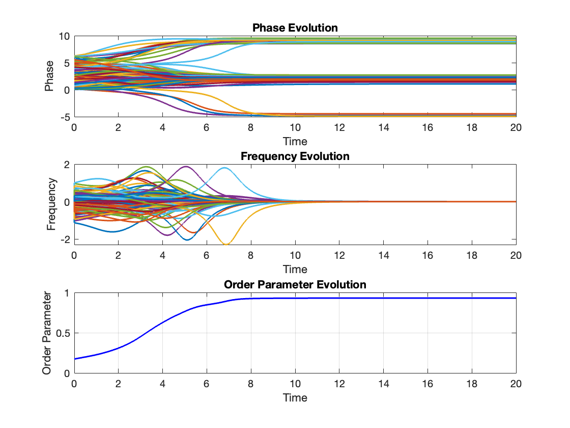
Figure 1: Phase, frequency, and order parameter evolution of $N=100$ oscillators in the first-order classical Kuramoto system (40). The coupling strength $\lambda=1.44$.

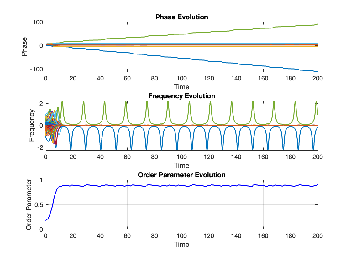
Figure 2: Phase, frequency, and order parameter evolution of $N=100$ oscillators in the first-order classical Kuramoto system (40). The coupling strength $\lambda=1.22$.

For the first-order classical Kuramoto system (40), we simulate $N=100$ oscillators, and present the evolution of phase, frequency, and order parameter in Fig. 1 ($\lambda=1.44$) and Fig. 2 ($\lambda=1.22$). For both figures, the natural frequencies are sampled from the normal distribution with mean $1$ and variance $0.25$, and then centered. For this realization of natural frequencies, the range $\omega_{\mathrm{M}}-\omega_{\mathrm{m}}$ is $2.3697$ and $\omega=1.2161$. The initial phases are sampled from the uniform distribution on $[0,2\pi)$.

We notice that the examples presented in Fig. 1 and Fig. 2 are consistent with Theorem 4.3 and Theorem 4.4: All modes of synchronization discussed in this paper, that is, (full) phase-locking, frequency, and order parameter synchronization, occur in Fig. 1, while all modes do not occur in Fig. 2. In particular, the order parameter $|Z(t)|=R(t)$ in Fig. 1 seems to converge to the limit $|Z^{*}|\approx 0.9305\geq\omega/\lambda\approx 0.8446$, so condition (5) is satisfied. Moreover, in Fig. 1 we can further check that the smallest upper bound for $|Z^{*}|=\lim_{t\to\infty}R(t)$ given by Corollary 5.5, namely, $1-\frac{1}{N}+\frac{1}{N}\sqrt{1-\frac{\omega^{2}}{\lambda^{2}}}\approx 0.9954$, is indeed an upper bound for the observed limit $|Z^{*}|\approx 0.9305$. On the other hand, Fig. 2 provides a concrete example where our proposed necessary condition of synchronization regarding critical coupling strength

$$\frac{\omega(N^{2}+1)}{N^{2}-N+\sqrt{2N}}\approx 1.2269>\lambda=1.22>1.2088\approx\frac{(\omega_{\mathrm{M}}-\omega_{\mathrm{m}})N}{2\sin(\theta_{\mathrm{opt}})+2(N-2)\sin\left(\frac{\theta_{\mathrm{opt}}}{2}\right)},$$

the one provided in [7]. That is, our proposed necessary condition rules out the possibility of synchronization while the one provided in [7] does not.

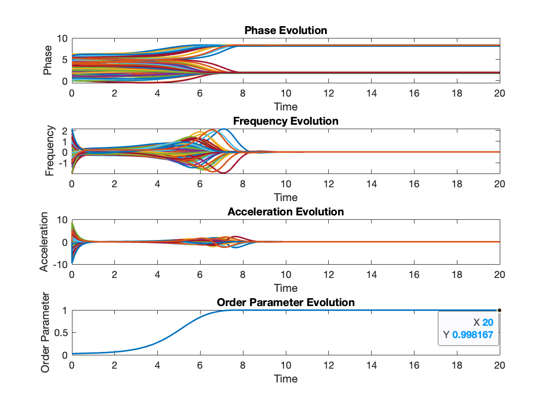
Figure 3: Phase, frequency, acceleration, and order parameter evolution of $N=100$ oscillators in the second-order classical Kuramoto system (28). The coupling strength $\lambda=8.88$.

For the second-order classical Kuramoto system (28), we simulate $N=100$ oscillators and present the evolution of phase, frequency, acceleration, and order parameter in Fig. 3. We choose $\lambda=8.88$, $m_{j}=1$, and $d_{j}=4.2144$ for all $j$; the natural frequencies are sampled from the normal distribution with mean $1$ and variance $0.25$, then centered. For this realization of natural frequencies, the range $\omega_{\mathrm{M}}-\omega_{\mathrm{m}}$ is $2.6961$ and $\omega=1.4798$. The initial phases are sampled from the uniform distribution on $[0,2\pi)$.

We notice that this example, presented in Fig. 3, is consistent with Theorem 4.5, Theorem 4.6, and Theorem 4.7 in the sense that (full) phase-locking, frequency, (exponential) acceleration and OP synchronization all happen in this case. In particular, for Theorem 4.7, the parameters satisfy the premises with, for example, $\epsilon=1/6$ and $\delta=1.9773\times 10^{-5}$; specifically, the observed OP limit $|Z^{\star}|=\lim_{t\to\infty}|Z(t)|\approx 0.998167>\frac{2}{3(1-\epsilon)}=0.8$. Moreover, Corollary 6.4 yields the upper bound $1-\frac{1}{N}+\frac{1}{N}\sqrt{1-\frac{\omega^{2}}{\lambda^{2}}}\approx 0.9999$ for $|Z^{\star}|$, which is also consistent with this example.

References

- [1] J. Baillieul and C. Byrnes, Geometric critical point analysis of lossless power system models, IEEE Transactions on Circuits and Systems, 29 (1982), pp. 724–737.
- [2] M. Breakspear, S. Heitmann, and A. Daffertshofer, Generative models of cortical oscillations: neurobiological implications of the Kuramoto model, Frontiers in Human Neuroscience, 4 (2010), p. 190.
- [3] J. C. Bronski, T. E. Carty, and S. E. Simpson, A matrix-valued Kuramoto model, Journal of Statistical Physics, 178 (2020), pp. 595–624.
- [4] V. Chandrasekar, M. Manoranjani, and S. Gupta, Kuramoto model in the presence of additional interactions that break rotational symmetry, Physical Review E, 102 (2020), p. 012206.
- [5] S.-H. Chen, C.-H. Hsia, and T.-Y. Hsiao, Complete and partial synchronization of two-group and three-group Kuramoto oscillators, SIAM Journal on Applied Dynamical Systems, 23 (2024), pp. 1720–1765.
- [6] L. M. Childs and S. H. Strogatz, Stability diagram for the forced Kuramoto model, Chaos: An Interdisciplinary Journal of Nonlinear Science, 18 (2008).
- [7] N. Chopra and M. W. Spong, On exponential synchronization of Kuramoto oscillators, IEEE transactions on Automatic Control, 54 (2009), pp. 353–357.
- [8] O. Coss, J. D. Hauenstein, H. Hong, and D. K. Molzahn, Locating and counting equilibria of the Kuramoto model with rank-one coupling, SIAM Journal on Applied Algebra and Geometry, 2 (2018), pp. 45–71.
- [9] F. De Smet and D. Aeyels, Partial entrainment in the finite Kuramoto-Sakaguchi model, Physica D: Nonlinear Phenomena, 234 (2007), pp. 81–89.
- [10] L. DeVille, Synchronization and stability for quantum Kuramoto, Journal of Statistical Physics, 174 (2019), pp. 160–187.
- [11] F. Dörfler and F. Bullo, On the critical coupling for Kuramoto oscillators, SIAM Journal on Applied Dynamical Systems, 10 (2011), pp. 1070–1099.
- [12] F. Dörfler, M. Chertkov, and F. Bullo, Synchronization in complex oscillator networks and smart grids, Proceedings of the National Academy of Sciences, 110 (2013), pp. 2005–2010.
- [13] V. Flovik, F. Macia, and E. Wahlström, Describing synchronization and topological excitations in arrays of magnetic spin torque oscillators through the Kuramoto model, Scientific reports, 6 (2016), p. 32528.
- [14] S. Gupta, A. Campa, and S. Ruffo, Kuramoto model of synchronization: equilibrium and nonequilibrium aspects, Journal of Statistical Mechanics: Theory and Experiment, 2014 (2014), p. R08001.
- [15] S.-Y. Ha and S.-Y. Ryoo, Asymptotic phase-locking dynamics and critical coupling strength for the Kuramoto model, Communications in Mathematical Physics, 377 (2020), pp. 811–857.
- [16] C.-H. Hsia, C.-Y. Jung, and B. Kwon, On the synchronization theory of Kuramoto oscillators under the effect of inertia, Journal of Differential Equations, 267 (2019), pp. 742–775.
- [17] T.-Y. Hsiao, Y.-F. Lo, and W. Wang, Synchronization in the quaternionic Kuramoto model, arXiv preprint arXiv:2309.01893, (2023).
- [18] T.-Y. Hsiao, Y.-F. Lo, and W. Wang, Synchronization in the complexified Kuramoto model, arXiv preprint arXiv:2502.20614, (2025).
- [19] M. Kassabov, S. H. Strogatz, and A. Townsend, Sufficiently dense Kuramoto networks are globally synchronizing, Chaos: An Interdisciplinary Journal of Nonlinear Science, 31 (2021).
- [20] Y. Kuramoto, Self-entrainment of a population of coupled non-linear oscillators, in International Symposium on Mathematical Problems in Theoretical Physics: January 23–29, 1975, Kyoto University, Kyoto/Japan, Springer, 1975, pp. 420–422.
- [21] E. Landau, Die Ungleichungen für zweimal differentiierbare Funktionen, vol. 6, AF Høst & Son, 1925.
- [22] L. D. Landau et al., On the theory of phase transitions, Zh. eksp. teor. Fiz, 7 (1937), p. 926.
- [23] H. S. Lee, B. J. Kim, and H. J. Park, Stability of twisted states in power-law-coupled Kuramoto oscillators on a circle with and without time delay, Physical Review E, 109 (2024), p. 064203.
- [24] S. Ling, R. Xu, and A. S. Bandeira, On the landscape of synchronization networks: A perspective from nonconvex optimization, SIAM Journal on Optimization, 29 (2019), pp. 1879–1907.
- [25] M. Lohe, Non-Abelian Kuramoto models and synchronization, Journal of Physics A: Mathematical and Theoretical, 42 (2009), p. 395101.
- [26] J. Lu and S. Steinerberger, Synchronization of Kuramoto oscillators in dense networks, Nonlinearity, 33 (2020), p. 5905.
- [27] M. Manoranjani, S. Gupta, D. Senthilkumar, and V. Chandrasekar, Generalization of the Kuramoto model to the Winfree model by a symmetry breaking coupling, The European Physical Journal Plus, 138 (2023), p. 144.
- [28] G. S. Medvedev and X. Tang, The Kuramoto model on power law graphs: synchronization and contrast states, Journal of Nonlinear Science, 30 (2020), pp. 2405–2427.
- [29] D. Mehta, N. S. Daleo, F. Dörfler, and J. D. Hauenstein, Algebraic geometrization of the Kuramoto model: Equilibria and stability analysis, Chaos: An Interdisciplinary Journal of Nonlinear Science, 25 (2015).
- [30] R. Ronge, M. A. Zaks, and T. Pereira, Continua and persistence of periodic orbits in ensembles of oscillators, Nonlinearity, 37 (2024), p. 055004.
- [31] H. Sakaguchi and Y. Kuramoto, A soluble active rotater model showing phase transitions via mutual entertainment, Progress of Theoretical Physics, 76 (1986), pp. 576–581.
- [32] S. Shinomoto and Y. Kuramoto, Phase transitions in active rotator systems, Progress of Theoretical Physics, 75 (1986), pp. 1105–1110.
- [33] R. Taylor, There is no non-zero stable fixed point for dense networks in the homogeneous Kuramoto model, Journal of Physics A: Mathematical and Theoretical, 45 (2012), p. 055102.
- [34] M. Thümler, S. G. Srinivas, M. Schröder, and M. Timme, Synchrony for weak coupling in the complexified Kuramoto model, Physical Review Letters, 130 (2023), p. 187201.
- [35] B. R. Trees, V. Saranathan, and D. Stroud, Synchronization in disordered Josephson junction arrays: Small-world connections and the Kuramoto model, Physical Review E—Statistical, Nonlinear, and Soft Matter Physics, 71 (2005), p. 016215.
- [36] J. Van Hemmen and W. Wreszinski, Lyapunov function for the Kuramoto model of nonlinearly coupled oscillators, Journal of Statistical Physics, 72 (1993), pp. 145–166.
- [37] S. Watanabe and S. H. Strogatz, Constants of motion for superconducting Josephson arrays, Physica D: Nonlinear Phenomena, 74 (1994), pp. 197–253.
- [38] K. Wiesenfeld, P. Colet, and S. H. Strogatz, Frequency locking in Josephson arrays: Connection with the Kuramoto model, Physical Review E, 57 (1998), p. 1563.
- [39] K. Xi, J. L. Dubbeldam, and H. X. Lin, Synchronization of cyclic power grids: equilibria and stability of the synchronous state, Chaos: An Interdisciplinary Journal of Nonlinear Science, 27 (2017).