Homotopy approach for scattering amplitude for running QCD coupling

Abstract

In this paper we proposed the homotopy approach for solving the nonlinear Balitsky-Kovchegov (BK) evolution equation with running QCD coupling. The approach consists of two steps. First, is the analytic solution to the nonlinear evolution equation for the simplified, leading twist kernel. Second, is the iteration procedure that allow us to calculate corrections analytically or semi-numerically. For the leading twist kernel it is shown that the first iteration leads to $\leq 1\%$ accuracy. The $\zeta=-\frac{4N_{c}}{b_{0}}Y\ln\left(\bar{\alpha}_{S}(1/Q^{2}_{s}(Y))/\bar{\alpha}_{S}\left(r^{2}\right)\right)$ ($r$ is the dipole size, $Q_{s}$ is the saturation scale) and geometric scaling behaviour of the scattering amplitude are discussed as well as the dependence on the value of the infrared cutoff.

I Introduction

In this paper we are going to continue our search for the regular iteration procedure of solving non-linear equations that govern QCD dynamics in the saturation region. Our general method is based on homotopy approachHE1 ; HE2 which we developed in our previous papers for the Balitsky-KovchegovBK equation for the scattering amplitudeCLMNEW and for the equation for the cross section of diffraction productionKOLE ; CGLM .

Basically, our approach consists of two stages. In the first stage we find the analytic or almost analytic solution to the non-linear equation with the simplified BFKLBFKL kernel which collects the main features of the saturation. In the second stage we develop the numerical computation to estimate the corrections to the first iteration.

In this paper we wish to expand our procedure to the case of running QCD coupling. The good news is that we know how to introduce the running QCD coupling into the non-linear equationRAL ; and that we know the main difficulties of the searching of the solution related to the violation of the geometric behaviour of the scattering amplitudeRUNAL .

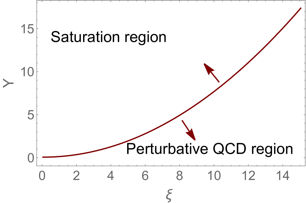
Figure 1: Saturation region of QCD for the elastic scattering amplitude. The critical line: $\frac{8N_{c}}{b}\,\,\frac{\chi\left(\gamma_{cr}\right)}{1\,-\,\gamma_{cr}}\,Y\,\equiv\,\,\xi^{2}_{s}\,\,=\,\,\xi^{2}\,$ is shown in red. The initial condition for scattering with the dilute system of partons (with proton) is given at $\xi_{s}=0$. The variable $\xi_{s}$ is defined as $\xi_{s}\,=\,\ln\left(Q^{2}_{s}(Y,b)/Q_{s}^{2}(Y=Y_{0},b)\right)$.

The detailed description of our approach is included in the next sections. Here we wish to discuss the kinematic region where we are looking for the solution and general assumptions that we make in fixing initial and boundary conditions. The nonlinear Balitsky-Kovchegov equation has the following formBK for the scattering amplitude of the dipole with size $r$:

$$\frac{\partial N\left(r,Y;\boldsymbol{b}\right)}{\partial\,Y}\,\,\, = \,\,\,\,\int\,\frac{d^{2}r_{1}}{2\pi}\,K\left(r;r_{1},r_{2}\right)\times\Big{\{}N\left(r_{1},Y;\boldsymbol{b}\,-\,\frac{1}{2}\,\boldsymbol{r}_{2}\right)\,+\,N\left(r_{2},Y;\boldsymbol{b}\,-\,\frac{1}{2}\,\boldsymbol{r}_{1}\right)\,-\,\,\,N\left(r,Y;\boldsymbol{b}\right)\,\,$$ (I.1)

$$- \,\,N\left(r_{1},Y;\boldsymbol{b}-\frac{1}{2}\,\boldsymbol{r}_{2}\right)\,N\left(r_{2},Y;\boldsymbol{b}-\frac{1}{2}\boldsymbol{r}_{1}\right)\Big{\}}$$

where $Y=\ln(1/x)$ is the rapidity of the incoming dipole; $N$ is the imaginary part of the scattering amplitude and $b$ is the impact parameter of this scattering process and $\boldsymbol{r}_{2}=\boldsymbol{r}-\boldsymbol{r}_{1}$. The BFKL kernel with running QCD coupling $K\left(r;r_{1},r_{2}\right)$ in the Balitsky prescriptionRAL has the following form

$$K_{rc}^{Bal}\left(r;r_{1},r_{2}\right)\,\,=\,\,\bar{\alpha}_{S}\left(r^{2}\right)\left\{\frac{r^{2}}{r^{2}_{1}\,r^{2}_{2}}\,\,+\,\,\frac{1}{r_{1}^{2}}\left(\frac{\bar{\alpha}_{S}\left(r^{2}_{1}\right)}{\bar{\alpha}_{S}\left(r^{2}_{2}\right)}\,-\,1\right)\,+\,\frac{1}{r_{2}^{2}}\left(\frac{\bar{\alpha}_{S}\left(r^{2}_{2}\right)}{\bar{\alpha}_{S}\left(r^{2}_{1}\right)}\,-\,1\right)\right\}$$ (I.2)

while in the Kovchegov-Weigert prescriptionRAL2 it has the following form

$$K_{rc}^{KW}\left(r;r_{1},r_{2}\right)\,\,=\,\,\bar{\alpha}_{S}\left(r^{2}_{1}\right)\left\{\frac{1}{r^{2}_{1}}\,\,-2\,\frac{\bar{\alpha}_{S}\left(r^{2}_{2}\right)}{\bar{\alpha}_{S}\left(R^{2}_{0}\right)}\,\frac{\boldsymbol{r}_{1}\cdot\boldsymbol{r}_{2}}{r_{1}^{2}r_{2}^{2}}\,+\,\frac{1}{r_{2}^{2}}\frac{\bar{\alpha}_{S}\left(r^{2}_{2}\right)}{\bar{\alpha}_{S}\left(r^{2}_{1}\right)}\right\}$$ (I.3)

with

$$R_{0}^{2}\left(r;r_{1},r_{2}\right)\,\,=\,r_{1}r_{2}\left(\frac{r_{2}}{r_{1}}\right)^{\frac{r_{1}^{2}+r_{2}^{2}}{r_{1}^{2}-r_{2}^{2}}-2\frac{r_{1}^{2}r_{2}^{2}}{\boldsymbol{r}_{1}\cdot\boldsymbol{r}_{2}}\,\frac{1}{r_{1}^{2}-r_{2}^{2}}}$$ (I.4)

Both prescriptions neglect different contributions. However, numerical studies KOVCUT indicate that the Balitsky prescription provides a closer result to the full answer, where no approximations are made. Therefore, we adopt the Balitsky prescription in our analysis.

In Eq. (I.2) and Eq. (I.3) $\alpha_{S}$ is the QCD coupling

$$\alpha_{S}\left(r^{2}\right)\,\,=\,\,\frac{\alpha_{S}\left(R^{2}\right)}{1\,\,+\,\,\frac{\alpha_{S}\left(R^{2}\right)}{4\pi b_{0}}\ln\left(R^{2}/r^{2}\right)}\,\,=\,\,\frac{4\pi}{b_{0}\,\ln\left(1/\left(r^{2}\,\Lambda^{2}_{QCD}\right)\right)}$$ (I.5)

and $\bar{\alpha}_{S}=N_{c}\alpha_{S}/\pi$ with $b_{0}=11N_{c}/3-2N_{f}/3$ for number of colours $N_{c}$ and the number of flavours $N_{f}$. $R$ is the arbitrary size (so called the renormalization point) which the physical observables do not depend on.

First we need to find the solution to the nonlinear equation in the vicinity of the saturation scale to specify the kinematic regions where we will attempt to solve the nonlinear equations.

In the vicinity of the saturation scale where $r^{2}\,\approx r^{2}_{1}\,\approx r^{2}_{2}\,\approx 1/Q^{2}_{s}$, we can consider that $\bar{\alpha}_{S}\left(r^{2}\right)\,=\,\bar{\alpha}_{S}\left(r^{2}_{1}\right)=\bar{\alpha}_{S}\left(r^{2}_{2}\right)$ . We can see that for $R=r$

$$\alpha_{S}\left(r^{2}_{i}\right)\,\,=\,\,\frac{\alpha_{S}\left(r^{2}\right)}{1\,\,+\,\,\frac{\alpha_{S}\left(r^{2}\right)}{4\pi b}\ln\left(r^{2}/r^{2}_{i}\right)}\,\,\,\,\xrightarrow{\ln\left(r^{2}/r^{2}_{i}\right)\,\ll\,ln\left(r^{2}\,\Lambda^{2}_{QCD}\right)}\,\,\,\,\alpha_{S}\left(r^{2}\right)$$ (I.6)

For $r^{2}\,\varpropto\,1/Q^{2}_{s}$ condition $|\ln\left(r^{2}_{i}\,Q^{2}_{s}\right)|\,\ll\,\ln\left(Q^{2}_{s}/\Lambda^{2}_{QCD}\right)$ determines the kinematic region which we call vicinity of the saturation scale. Using this simplification the kernel of Eq. (I.1) takes the form:

$$K\left(r;r_{1},r_{2}\right)\,\,\,=\,\,\bar{\alpha}_{S}\left(r^{2}\right)\,\frac{r^{2}}{r^{2}_{1}\,r^{2}_{2}}$$ (I.7)

The second simplification stems from the observation that for the equation for the saturation scale $Q_{s}$ we do not need to know the precise form of the non-linear term GLR ; MUT ; MUPE (see also Ref.KOLEB ). Therefore, to find $Q_{s}$ as well as the behaviour of the amplitude in the vicinity of the saturation scale we need to solve the linear BFKL equation, but using the procedure which will be suitable for the solution of the non-linear equation with a general non-linear term. It is enough to use the semiclassical approximation for the amplitude $N\left(r,Y;b\right)$, which has the form

$$N_{A}\left(Y,\xi\right)\,\,=\,\,e^{S\left(Y,\xi\right)}\,\,=\,\,e^{\omega\left(Y,\xi\right)\,Y\,+\,\left(1-\gamma\left(Y;\xi\right)\right)\,\xi\,+\,S_{0}}$$ (I.8)

where $\xi\,=\,\ln\left(r^{2}Q^{2}_{s}\left(Y=Y_{0};b\right)\right)$. In Eq. (I.8) we are searching for functions $\omega\left(Y,\xi\right)$ and $\gamma\left(Y,\xi\right)$ which are smooth functions of both arguments (see Ref.KOLEB for details). Plugging in the linear BFKL equation the solution of Eq. (I.8) and taking into account that function $(r^{2})^{f}\equiv\exp\left(f\,\xi\right)$ is the eigenfunction of the BFKL equation, viz.:

$$\bar{\alpha}_{S}\left(r^{2}\right)\int\,\frac{d^{2}r_{1}}{2\pi}\,K\left(r;r_{1},r_{2}\right)\,(r^{2}_{1})^{f}\,\,=\,\,\bar{\alpha}_{S}\left(r^{2}\right)\chi\left(f\right)\,(r^{2})^{f}\,\,\mbox{with}\,\,\,\chi\left(f\right)\,\,=\,\,2\,\psi(1)-\psi(f)-\psi(1-f)$$

$$\,\,\mbox{where}\,\,\psi(z)=d\ln\Gamma(z)/dz\,\mbox{ and }\,\Gamma(z)\,\mbox{ is Euler gamma function}$$ (I.9)

we obtain that

$$\omega\left(Y,\xi\right)\,\,\,=\,\,\bar{\alpha}_{S}\left(\xi\right)\,\chi\left(\gamma\left(Y,\xi\right)\right)$$ (I.10)

This solution has a form of wave-package and the critical line is the specific trajectory for this wave-package which coincides with the its front line. In other words, it is the trajectory on which the phase velocity ($v_{ph}$) for the wave-package is the same as the group velocity ($v_{gr}$). The equation $v_{gr}\,=\,v_{ph}$ has the folowing form for Eq. (I.10)

$$v_{ph}\,\,=\,\,\bar{\alpha}_{S}\left(r^{2}\right)\frac{\chi\left(\gamma_{cr}\right)}{1\,-\,\gamma_{cr}}\,\,\,=\,\,\,-\bar{\alpha}_{S}\left(r^{2}\right)\chi^{\prime}\left(\gamma_{cr}\right)\,\,=\,\,v_{gr}$$ (I.11)

with the solution $\gamma_{cr}\,=\,0.37$. Eq. (I.11) can be translated into the following equation for the critical trajectory

$$\frac{d\xi\left(Y\right)}{dY}\,\,=\,\,v_{ph}\,\,=\,\,\bar{\alpha}_{S}\left(\xi\right)\,\frac{\chi\left(\gamma_{cr}\right)}{1\,-\,\gamma_{cr}}$$ (I.12)

with the solution

$$\frac{8N_{c}}{b_{0}}\,\,\frac{\chi\left(\gamma_{cr}\right)}{1\,-\,\gamma_{cr}}\,Y\,\equiv\,\,\xi^{2}_{s}\,\,=\,\,\xi^{2}\,\,-\,\,\xi^{2}_{0}\,\,\$$ (I.13)

where $\xi_{0}\,=\,\ln\left(Q^{2}_{s}\left(Y=Y_{0};b\right)/\Lambda^{2}_{QCD}\right)$ and $\xi_{s}\,=\,\ln\left(Q^{2}_{s}(Y,b)/Q_{s}^{2}(Y=Y_{0},b)\right)$. For simplicity we choose $Q_{s}^{2}(Y=Y_{0},b)=\Lambda^{2}_{QCD}$. It means that we model the DIS with the proton by the scattering of dipole $r$ with the dipole size is equal to $R=1/\Lambda_{QCD}$.

Eq. (I.13) results in the saturation moment $Q_{s}^{2}(Y)$ which is equal to

$$Q^{2}_{s}\left(Y,b\right)\,\,=\,\,Q^{2}_{s}\left(Y=Y_{0},b\right)\,e^{\sqrt{\frac{8N_{c}}{b_{0}}\,\frac{\chi\left(\gamma_{cr}\right)}{1\,-\,\gamma_{cr}}\,Y}}\$$ (I.14)

We note that the dependence of $Q_{s}$ on $Y$ changes from a linear behavior in the fixed coupling case to the form given by Eq. (I.14) in the running coupling case. This change slows down the evolution of the scattering amplitude.

The behaviour of the scattering amplitude in the vicinity of the saturation scale has been found in Refs.IIM ; MUT ; KOLEB and it has the form:

$$N\left(Y,\xi;b\right)\,\,=\,\,N_{0}\left(r^{2}\,Q^{2}_{s}\left(Y,b\right)\right)^{\bar{\gamma}}~~~~\mbox{with}~~~\bar{\gamma}=1-\gamma_{cr}$$ (I.15)

One can see that we have a geometric scaling behaviour for the scattering amplitude in the vicinity of the saturation scale. Eq. (I.15) gives us the boundary condition for the nonlinear equation, viz.:

$$N\left(Y,\xi=-\xi_{s};b\right)\,=\,N_{0};\,\,\,\,\,\,\,\,\,\,\,\frac{\partial N\left(Y,\xi=-\xi_{s};b\right)}{\partial\xi}\,\,=\,\,\,\bar{\gamma}\,\,N_{0}$$ (I.16)

We wish to note that in the region of perturbative QCD (see Fig. 1) the scattering amplitude is the solution to the linear BFKL equation:

$$\frac{\partial N^{\tiny{\rm BFKL}}\left(r,Y;\boldsymbol{b}\right)}{\partial\,Y}\,=\int\,\frac{d^{2}r_{1}}{2\pi}\,K\left(r;r_{1},r_{2}\right)\Big{\{}N^{\tiny{\rm BFKL}}\left(r_{1},Y;\boldsymbol{b}\,-\,\frac{1}{2}\,\boldsymbol{r}_{2}\right)\,+\,N^{\tiny{\rm BFKL}}\left(r_{2},Y;\boldsymbol{b}\,-\,\frac{1}{2}\,\boldsymbol{r}_{1}\right)\,-\,\,\,N^{\tiny{\rm BFKL}}\left(r,Y;\boldsymbol{b}\right)\Big{\}}$$ (I.17)

The initial condition for this equation is the Born Approximation (the exchange of two gluons) for the scattering of the dipole with the size $r$ with the dipole with the size $R=1/\Lambda_{QCD}$.

We have to specify the region of $r_{\perp}$ which we are dealing with in the saturation region $r^{2}_{\perp}\,Q^{2}_{s}\left(Y,b\right)\,>\,1$. As has been noted in Refs.GOST ; BEST actually for very large $r_{\perp}$ the non-linear corrections are not important and we have to solve linear BFKL equation. This feature can be seen directly from the eigenfunction of this equation. Indeed, the eigenfunction (the scattering amplitude of two dipoles with sizes $r_{\perp}\equiv x_{10}$ and $R$) has the following form LIP

$$\phi_{\gamma}\left(\boldsymbol{r}_{\perp},\boldsymbol{R},\boldsymbol{b}\right)\,\,\,=\,\,\,\left(\frac{r^{2}\,R^{2}}{\left(\boldsymbol{b}+\frac{1}{2}(\boldsymbol{r}_{\perp}-\boldsymbol{R})\right)^{2}\,\left(\boldsymbol{b}-\frac{1}{2}(\boldsymbol{r}_{\perp}-\boldsymbol{R})\right)^{2}}\right)^{\gamma}\,\xrightarrow{b\gg\,r,R}\left(\frac{R^{2}r^{2}}{b^{4}}\right)^{\gamma}~~\mbox{with}\,\,0\,<\,Re\,\gamma\,<\,1$$ (I.18)

One can see that for $r_{\perp}=x_{10}\,>\,min[R,b]$, $\phi_{\gamma}$ starts to be smaller and the non-linear term in the BK equation could be neglected. The typical process, that we bear in mind, is the deep inelastic scattering(DIS) with a nucleus at $Q^{2}\,\geq\,1GeV^{2}$ and at small values of $x$. In our previous papersCLMNEW ; CGLM we have commented on impact parameter behaviour for the scattering with nucleus.

In our paper we can distinguish three parts. The first one is the brief discussion of the solution to the nonlinear evolution equation for the model leading twist BFKL kernel (section II and III). In these sections we discuss the main results of Ref.RUNAL and present the detailed analysis of self-similar solution to this equation. These sections contain the main theoretical basis for the first stage of our approach: finding an analytic or almost analytic solution to the non-linear equation. In section IV-VI we proposed the homotopy approach for the leading twist BFKL kernel. We demonstrated that the first iteration can be done based on the results of section III and estimates the next corrections. It turns out that the second iteration gives the solution within accuracy of several percents. Sections VIII and IX present our homotopy approach to the nonlinear equation with the general BFKL kernel. We observe that we need to make two iterations to reach a several percents accuracy. We show that we can suggest a pure analytic solution at the first iteration. In the conclusion we summarize our results and outline the problems that we faced developing our approach.

II The main features of the nonlinear equation for the leading twist BFKL kernel

In this section we briefly review the main result of Ref.RUNAL on the solution to the nonlinear equation with the simplified BFKL kernel. Following Ref. LETU we simplify the kernel by taking into account only log contributions. In other words, we would like to consider only leading twist contribution to the BFKL kernel, which contains all twists. Actually we have two types of the logarithmic contributions: $\ln\left(r^{2}\Lambda^{2}_{QCD}\right)$ for $r^{2}\,\ll\,1/Q^{2}_{s}$ and $\ln\left(r^{2}\,Q^{2}_{s}\right)$ for $r^{2}\,>\,1/Q^{2}_{s}$. In the saturation region we are dealing with the second kind of logs (see Refs.CLMNEW ; CGLM ). They come from the decay of the large size dipole into one small size dipole and one large size dipole. However, the size of the small dipole is still larger than $1/Q_{s}$. It turns out that $\bar{\alpha}_{S}$ depends on the size of produced dipole, if this size is the smallest one. It follows directly from Eq. (I.2) in the kinematic regions: $r\approx r_{2}\,\gg\,r_{1}\,\,\gg\,1/Q_{s}$ and $r\approx r_{1}\,\gg\,r_{2}\,\,\gg\,1/Q_{s}$ (see Ref. MURC for additional arguments). This observation can be translated in the following form of the kernel

$$\int d^{2}r^{\prime}\,K\left(r,r^{\prime}\right)\,\,\rightarrow\,\pi\,\int^{r^{2}}_{1/Q^{2}_{s}(Y,b)}\frac{\bar{\alpha}_{S}\left(r^{2}_{1}\right)dr^{2}_{1}}{r^{2}_{1}}\,\,+\,\,\pi\,\int^{r^{2}}_{1/Q^{2}_{s}(Y,b)}\frac{\bar{\alpha}_{S}\left(r^{2}_{2}\right)dr^{2}_{2}}{r^{2}_{2}}$$ (II.1)

One can see that this kernel leads to the $\left(\int^{r^{2}}_{1/Q^{2}_{s}(Y,b)}\frac{\bar{\alpha}_{S}\left(r^{2}_{1}\right)dr^{2}_{1}}{r^{2}_{1}}\right)^{n}$-contributions. Introducing a new function

$$\tilde{N}\left(r,Y;b\right)\,\,=\,\,\int\limits^{r^{2}}_{1/Q^{2}_{s}}dr^{\prime 2}\,\frac{\bar{\alpha}_{S}\left(r^{\prime 2}\right)}{r^{\prime 2}}\,N\left(r^{\prime},Y;b\right)$$ (II.2)

one obtain the following equation

$$\frac{\partial N\left(r,Y;b\right)}{\partial Y}\,\,=\,\,\tilde{N}\left(r,Y;b\right)\,\Big{(}1\,\,-\,\,N\left(r,Y;b\right)\Big{)}$$ (II.3)

Introducing a new variable

$$l\,\,=\,\,\int^{r^{2}}\,dr^{\prime 2}\frac{\bar{\alpha}_{S}\left(r^{\prime 2}\right)}{r^{\prime 2}}\,\,=\,\,-\frac{4N_{c}}{b_{0}}\,\ln\Big{(}4N_{c}/\left(b_{0}\,\bar{\alpha}_{S}\left(r^{2}\right)\right)\Big{)}\,\,=\,\,-\frac{4N_{c}}{b_{0}}\,\ln\left(\bar{\xi}\right)$$ (II.4)

with $\bar{\xi}\,=\,-\ln\left(r^{2}\,\Lambda^{2}_{QCD}\right)\,\equiv\,-\xi$ and new function $\Omega\left(r,Y;b\right)$

$$N\left(r,Y;b\right)\,\,=\,\,1\,\,\,-\,\,e^{-\Omega\left(r,Y;b\right)}$$ (II.5)

we obtain the following equation

$$\frac{\partial^{2}\Omega\left(r,Y;b\right)}{\partial Y\partial l}\,\,=\,\,1\,\,\,-\,\,\,e^{-\Omega\left(r,Y;b\right)}$$ (II.6)

One can see that Eq. (II.6) has the same form as the nonlinear equation with the fixed QCD couplingCLMNEW ; CGLM but $\xi$ is replaced by $l$.

Below we will often use the variable $l-l_{s}$ which is equal to

$$l\,-\,l_{s}\,\,=\,\,\int\limits^{r^{2}}_{1/Q^{2}_{s}}dr^{\prime 2}\frac{\bar{\alpha}_{S}\left(r^{\prime 2}\right)}{r^{\prime 2}}\,\,=\,\,-\frac{4\,N_{c}}{b_{0}}\ln\left(\frac{-\xi}{\xi_{s}}\right)$$ (II.7)

III Solutions to the simplified equation

III.1 Solution for $\Omega\,\gg\,1$

Searching for the solution to Eq. (II.6) we start with finding the asymptotic behaviour of $\Omega$ at large values of $Y$ and $l$. In this kinematic region we expect that that $\Omega$ will be large since the scattering amplitude approaches to unity. Hence, in this region Eq. (II.6) degenerates to a very simple equation

$$\frac{\partial^{2}\Omega\left(Y,l;b\right)}{\partial Y\partial l}\,\,=\,\,1$$ (III.1)

with obvious solution:

$$\tilde{\Omega}_{\infty}\left(Y,l;b\right)\,\,=\,\,Y\,l\,+\,F\left(Y\right)\,+\,G\left(l\right)$$ (III.2)

Functions $F$ and $G$ should be found from the initial conditions of Eq. (I.16) and they take the form

$$\tilde{\Omega}_{\infty}\left(Y,l;b\right)\,\,=\,\,Y\,\left(l-l_{s}\right)\,-\,\bar{\gamma}\,\Omega_{0}\,\left(e^{-\frac{b_{0}}{4N_{c}}l}\,-\,e^{-\frac{b_{0}}{4N_{c}}l_{s}}\right)\,+\,\frac{1}{4\,\kappa}\left(e^{-\frac{b_{0}}{2N_{c}}l}\,-\,e^{-\frac{b_{0}}{2N_{c}}l_{s}}\right)\,\,+\,\,\Omega_{0}$$ (III.3)

where $l_{s}\,\,=\,\,-\,\frac{4\,N_{c}}{b_{0}}\ln\xi_{s}$ and $\kappa=\chi\left(\gamma_{cr}\right)/(1-\gamma_{cr})$.

Eq. (III.3) at $\bar{\xi}\,\to\,\xi_{s}$ leads to

$$\tilde{\Omega}_{\infty}\left(Y,l;b\right)\,\,\xrightarrow{\bar{\xi}-\xi_{s}\,\ll\,\xi_{s}}\,\,\Omega_{0}\,+\,\bar{\gamma}\Omega_{0}\left(\xi+\xi_{s}\right)\,\,=\,\,\Omega_{0}\,\,+\,\,\,\bar{\gamma}\,\Omega_{0}\,z$$ (III.4)

showing the geometric scaling behaviour. Hence, we can hope that the solution will show the geometric scaling behaviour in the vicinity of the saturation scale. Note, that Eq. (III.3) does not depend on $l-l_{s}$ except the first term.

III.2 Traveling wave solution

Eq. (II.6) has general traveling wave solution (see Ref.MATH formula 3.5.3) which can be found noticing that $\Omega\left(Y,l;b\right)\,\equiv\,\phi\left(\eta\equiv a\,Y+b\,l;b\right)$ reduced the equation to

$$a\,b\frac{d^{2}\phi\left(\eta;b\right)}{d\eta^{2}}\,\,=\,\,1-e^{-\phi\left(\eta;b\right)}$$ (III.5)

The general solution of Eq. (III.5) has the form

$$\int^{\phi}_{\phi_{0}}\frac{d\phi^{\prime}}{\sqrt{c\,+\,\frac{1}{2\,a\,b}\Big{(}\phi^{\prime}-1+e^{-\phi^{\prime}}\Big{)}}}\,\,=\,\,\eta\,\,=\,\,a\,Y\,+\,b\,(l-l_{s})$$ (III.6)

where $c,\phi_{0},a$ and $b$ are arbitrary constants that should be found from the initial and boundary conditions.

The initial conditions of Eq. (I.16) can be written in terms of $Y$ and $l$ variables as

$$\phi\left(\eta\,=\,aY;b\right)\,\,=\,\,\,\phi_{0}\,;\,\,\,\,\,\,\,\,\,\,\,\,\phi^{\prime}_{\eta}\left(\eta\,=\,aY+b(l-l_{s});b\right)\Bigg{|}_{l=ls}\,\,=\,\,-\frac{1}{2}\,\phi_{0}\,\xi_{s}$$ (III.7)

It should be mentioned that the variable $\eta$ is not the scaling variable $z\,=\,\ln\left(\tau\right)\,=\,\xi_{s}-\bar{\xi}$ with $\xi_{s}=\sqrt{\frac{8N_{c}\kappa}{b_{0}}\,Y}$. One can see that we cannot satisfy the initial conditions of Eq. (III.7). Indeed, even to satisfy the first of Eq. (III.7) we need to choose $\eta=0$ on the critical line. As you see we cannot do this with $a$ and $b$ being constants. The second equation depends on $Y$, but not on $\eta$, making impossible to satisfy this condition in the framework of traveling wave solution.

If we try to find a solution which depends on $z$ ($\Omega\left(Y;r^{2};b\right)=\Omega\left(z;b\right)$) we obtain the following equation (using $\kappa\,=\,4$ and the variable $\tilde{z}\,=\,\sqrt{\frac{16N_{c}}{b_{0}}}\,z$)

$$\sqrt{\frac{16N_{c}}{b_{0}}}\frac{\tilde{z}}{\sqrt{2\,Y}}\,\frac{d^{2}\Omega\left(\tilde{z};b\right)}{d\,\tilde{z}^{2}}\,\,+\,\,\frac{d^{2}\Omega\left(\tilde{z};b\right)}{d\,\tilde{z}^{2}}\,\,=\,\,1\,\,-\,\,e^{-\Omega\left(\tilde{z};b\right)}$$ (III.8)

Therefore, only in the vicinity of the critical line where $\sqrt{\frac{16N_{c}}{b_{0}}}\,\tilde{z}\,\ll\,\sqrt{2\,Y}$ we can expect the geometric scaling behaviour of the scattering amplitude. It should be stressed that at large value of $Y$ the region where we have the geometric scaling behaviour becomes rather large. Neglecting the first term in Eq. (III.8) we obtain the equation in the same form as for frozen $\alpha_{S}$. It is easy to find the solution to this equation that satisfies the initial condition of Eq. (I.16). Actually, the condition $\sqrt{\frac{16N_{c}}{b_{0}}}\,\tilde{z}\,\ll\,\sqrt{2\,Y}$ can be rewritten as $\alpha_{S}\left(Q^{2}_{s}\right)\,\ln\left(r^{2}Q^{2}_{s}\right)\,\ll\,1$ and it shows the region in which we can consider the running QCD coupling as being frozen at $r^{2}=1/Q^{2}_{s}$.

III.3 Self-similar solution

Generally speaking (see Ref.MATH formulae 3.4.1.1 and 3.5.2) Eq. (II.6) has a self similar (functional separable) solution $\Omega\left(Y,l;b\right)\,=\,\Omega\left(\zeta;b\right)$ with

$$\zeta\,\,=\,\,Y\,l$$ (III.9)

For function $\Omega\left(\zeta;b\right)$ we can reduce Eq. (II.6) to the ordinary differential equation

$$\zeta\,\,\frac{d^{2}\Omega\left(\zeta;b\right)}{d\zeta^{2}}\,\,+\,\,\frac{d\,\Omega\left(\zeta;b\right)}{d\zeta}\,\,=\,\,1\,\,-\,\,e^{-\Omega\left(\zeta;b\right)}$$ (III.10)

The initial condition of Eq. (I.16) can be rewritten in the form

$$\Omega\left(\zeta=Y\,l_{s};b\right)\,\, = \,\,\Omega_{0};\,\,\,\,\,\,\,\,\,\,\,$$ (III.11)

$$\frac{d\Omega\left(\zeta=Y\,l_{s};b\right)}{d\zeta}\,\, = \,\,2\kappa\,\bar{\gamma}\,\Omega_{0}/\xi_{s}\,\,=\,\,2\kappa\,\bar{\gamma}\,\Omega_{0}\Big{/}\sqrt{\frac{8N_{c}\kappa}{b_{0}}\,Y}$$

Generally speaking we cannot satisfy Eq. (III.11) using the solution of Eq. (III.10) since these conditions depend not only on $\zeta$ but on extra variable $Y$. However, at large value of $Y$ one can see that Eq. (III.11) degenerates to

$$\Omega\left(\zeta=0;b\right)\,\,=\,\,\Omega_{0};\,\,\,\,\,\,\,\,\,\,\,\frac{d\Omega\left(\zeta=0;b\right)}{d\zeta}\,\,=\,\,0;$$ (III.12)

Solution to Eq. (III.10) we can find starting from $\Omega\gg 1$. Eq. (III.10) takes the form:

$$\zeta\,\,\frac{d^{2}\Omega^{(0)}\left(\zeta;b\right)}{d\zeta^{2}}\,\,+\,\,\frac{d\Omega^{(0)}\left(\zeta;b\right)}{d\zeta}\,\,=\,\,1$$ (III.13)

with the solution:

$$\frac{d\Omega^{(0)}\left(\zeta;b\right)}{d\zeta}\,=\,1\,-\,\frac{c_{1}}{\zeta};~~~~~~\Omega^{(0)}\left(\zeta;b\right)\,=\,\zeta\,+c_{2}-c_{1}\ln\zeta$$ (III.14)

Constants $c_{1}$ and $c_{2}$ have to be found from the boundary conditions of Eq. (III.12). One can see that $c_{1}$ is equal to zero and $c_{2}=\Omega_{0}-Y\,l_{s}$ if $\Omega_{0}\,\ll\,1$. Note that Eq. (III.1) has as a solution the arbitrary function of Y. Hence that first iteration gives the solution which is the function of

$$\zeta=Y\,\left(l-l_{s}\right)$$ (III.15)

We assume the iterations of Eq. (III.10) lead to function which depends on these $\zeta$. Actually this feature follows from section II if we assume that

$$\tilde{N}\left(r,Y;b\right)\,\,=\,\,\int\limits^{r^{2}}_{1/Q^{2}_{s}}dr^{\prime 2}\,\frac{\bar{\alpha}_{S}\left(r^{\prime 2}\right)}{r^{\prime 2}}\,N\left(r^{\prime},Y;b\right)\,\,=\,\,\int\limits^{l-l_{s}}dl^{\prime}N\left(r^{\prime},Y;b\right)$$ (III.16)

Note that for $N\to 1$ Eq. (III.16) is valid. Generally Eq. (III.16) means that we are looking for the solution $\Omega\left(Y,l-l_{s};b\right)$.

Bearing Eq. (III.16) in mind we can rewrite Eq. (II.6) in the form

$$\frac{\partial^{2}\Omega\left(Y,l-l_{s};b\right)}{\partial Y\partial(l-l_{s})}\,\,=\,\,1\,\,\,-\,\,\,e^{-\Omega\left(Y,l-l_{s};b\right)}$$ (III.17)

Eq. (III.17) can be rewritten in the form of Eq. (III.10) for $\zeta=Y\,(l-l_{s})$.

For the second iteration we have $\Omega\,=\,\Omega^{(0)}\,\,+\,\,\Omega^{(1)}$ with the following equation for $\Omega^{(1)}$:

$$\zeta\,\,\frac{d^{2}\Omega^{(1)}\left(\zeta;b\right)}{d\zeta^{2}}\,\,+\,\,\frac{d\Omega^{(1)}\left(\zeta;b\right)}{d\zeta}\,\,=\,\,-\,\,e^{-\Omega^{(0)}\left(\zeta;b\right)}$$ (III.18)

Searching $\frac{d\Omega^{(1)}\left(\zeta;b\right)}{d\zeta}$ in the form:

$$\frac{d\Omega^{(1)}\left(\zeta;b\right)}{d\zeta}=\frac{1}{\zeta}C\left(\zeta\right)$$ (III.19)

we have

$$\frac{d\Omega^{(1)}\left(\zeta;b\right)}{d\zeta}=-\frac{1}{\zeta}\int^{\zeta}_{0}d\zeta^{\prime}\,e^{-\Omega^{(0)}\left(\zeta^{\prime};b\right)}\,=\,-\,\frac{1}{\zeta}e^{-\Omega_{0}}\left(1\,+\,\sinh(\zeta)\,-\,\cosh(\zeta)\right)$$ (III.20)

From Eq. (III.20) we have for $\Omega^{(1)}\left(\zeta;b\right)$:

$$\Omega^{(1)}\left(\zeta;b\right)=-\int^{\zeta}_{0}d\zeta^{\prime}\frac{d\Omega^{(1)}\left(\zeta^{\prime};b\right)}{d\zeta^{\prime}}\,\,+\,\,c_{3}=-e^{-\Omega^{(0)}}\underbrace{\left(-\text{Chi}(\zeta)+\log(\zeta)+\text{Shi}(\zeta)+\gamma\right)}_{\zeta-\frac{1}{4}\zeta^{2}+\mathcal{O}\left(\zeta^{3}\right)}\,\,+\,\,c_{3}$$ (III.21)

where $c_{3}$ is a constant which we need to find from the initial and boundary conditions. In Eq. (III.21) Chi$\left(\zeta\right)$ and Shi$\left(\zeta\right)$ are the hyperbolic sine and cosine integrals (see Ref.RY formula 8.22) and $\gamma$ is the Euler’s constant (see Ref.RY formula 9.72). Using the expansion at small $\zeta$ we can see that $c_{3}=0$.

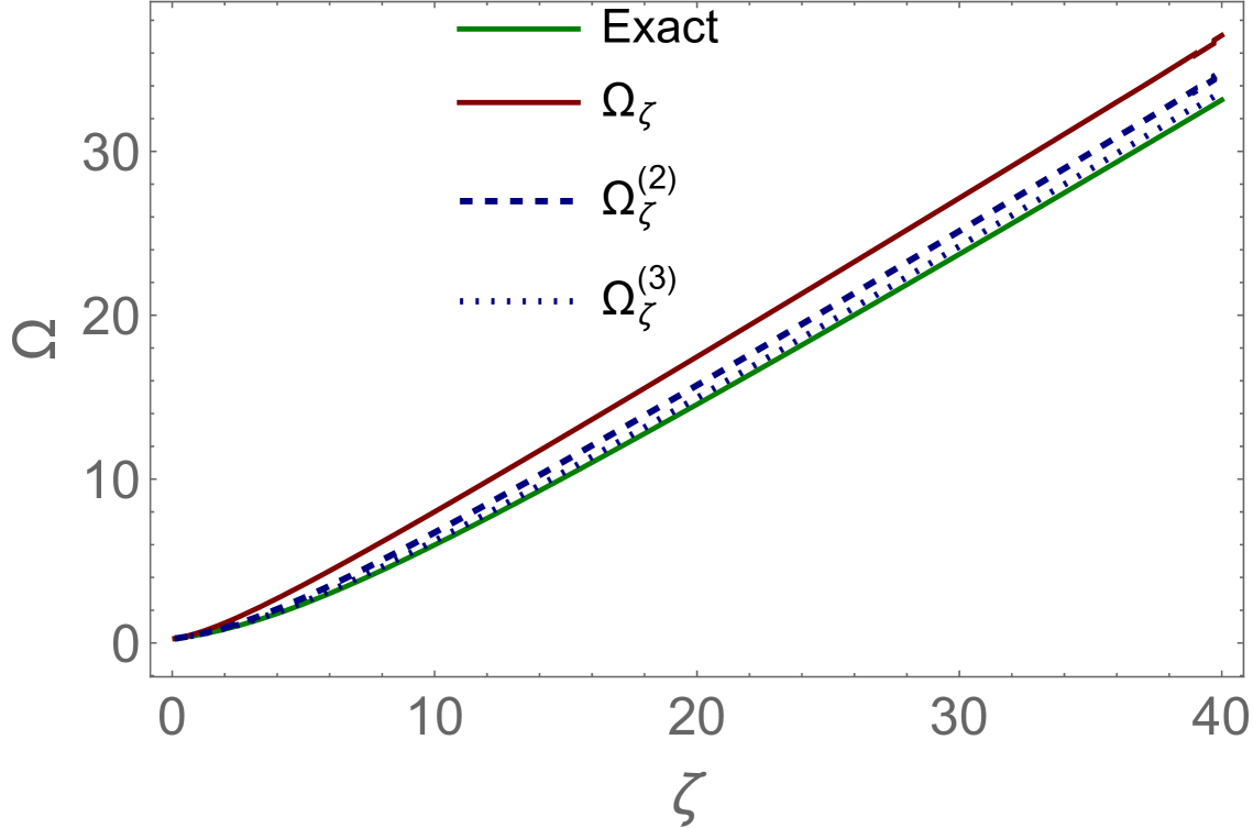
Figure 2: $\Omega\left(\zeta\right)$ versus $\zeta$. The exact solution to Eq. (III.10) with $\Omega_{0}=0.25$. $\Omega_{\zeta}=\Omega^{(0)}+\Omega^{(1)}$ from Eq. (III.14) and Eq. (III.18). $\Omega^{(2)}_{\zeta}\,=\,\Omega_{\zeta}+\Omega^{(2)}$, while $\Omega^{(3)}_{\zeta}\,=\,\Omega^{(2)}_{\zeta}+\Omega^{(3)}$. $\Omega^{(2)}$ and $\Omega^{(3)}$ are given by Eq. (III.22) and Eq. (III.23).

III.4 Numerical solution

In Fig. 2 we plot the exact solution to Eq. (III.10) with the initial conditions of Eq. (III.12) with $\Omega_{0}=0.25$ and $\Omega_{\zeta}=\Omega^{(0)}+\Omega^{(1)}$ taking from Eq. (III.14) and Eq. (III.18). One sees that our analytical approximation is not quite good. We need to find the next iteration of Eq. (III.18): $\Omega^{(2)}$. The equation for $\Omega^{(2)}$ takes the form:

$$\frac{d}{d\,\zeta}\left(\zeta\frac{d}{d\zeta}\Omega^{(2)}\left(\zeta;b\right)\right)\,\,=\,\,\,e^{-\Omega^{(0)}\left(\zeta;b\right)}\left(1-e^{-\Omega^{(1)}\left(\zeta;b\right)}\right)$$ (III.22)

with the initial conditions: $\Omega^{(0)}\left(\zeta=0;b\right)=0$ and $\frac{d\Omega^{(0)}\left(\zeta;b\right)}{d\zeta}|_{\zeta=0}=0$. Note, that we keep in the exponent since from Fig. 2 we see that $\Omega^{(1)}>1$. The calculated $\Omega^{(2)}$ is shown in Fig. 2. One can see that we need to make more iteration. The general expression for $i+1$ iteration is

$$\frac{d}{d\,\zeta}\left(\zeta\frac{d}{d\zeta}\Omega^{(i+1)}\left(\zeta;b\right)\right)\,\,=\,\,\,\exp\left(-\sum^{i-1}_{l=0}\Omega^{(l)}\left(\zeta;b\right)\right)\left(1-e^{-\Omega^{(i)}\left(\zeta;b\right)}\right)$$ (III.23)

The solution to Eq. (III.23) with zero initial conditions has the form:

$$\Omega^{(i+1)}\left(\zeta;b\right)\,\,=\,\,\int\limits^{\zeta}_{0}dt\ln\left(\frac{\zeta}{t}\right)\,\exp\left(-\sum_{l=0}^{i-1}\Omega^{(l)}\left(t;b\right)\right)\,\left(1-e^{-\Omega^{(i)}\left(t;b\right)}\right)$$ (III.24)

From Fig. 2 one can see that the calculation of $\Omega^{(3)}$ provides a good description of the numerical solution for $\Omega_{0}=0.25$.

IV Homotopy approach: first iteration.

The homotopy method we can use for the general equation:

$$\mathscr{L}[u]+\mathscr{N_{L}}[u]=0$$ (IV.1)

where the linear part $\mathscr{L}[u]$ is a differential or integral-differential operator, but non-linear part $\mathscr{N_{L}}[u]$ has an arbitrary form. As a solution, we introduce the following equation for the homotopy function ${\mathscr{H}}\left(p,u\right)$:

$${\mathscr{H}}\left(p,u\right)\,\,=\,\,\mathscr{L}[u_{p}]\,+\,p\,\mathscr{N_{L}}[u_{p}]\,\,=\,\,0$$ (IV.2)

Solving Eq. (IV.2) we reconstruct the function

$$u_{p}\left(Y,\boldsymbol{x}_{10},\boldsymbol{b}\right)\,\,=\,\,u_{0}\left(Y,\boldsymbol{x}_{10},\boldsymbol{b}\right)\,\,+\,\,p\,u_{1}\left(Y,\boldsymbol{x}_{10},\boldsymbol{b}\right)\,+\,p^{2}\,u_{2}\left(Y,\boldsymbol{x}_{10},\boldsymbol{b}\right)\,\,+\,\,\dots$$ (IV.3)

with $\mathscr{L}[u_{0}]=0$. Eq. (IV.3) gives the solution of the non-linear equation at $p=1$. The hope is that several terms in series of Eq. (IV.3) will give a good approximation in the solution of the non-linear equation.

As we have mentioned in the introduction the main idea of the homotopy approach is to find the first iteration or in other words, to introduce $\mathscr{L}[u_{p}]$ as the solution to the equation

$$\mathscr{L}[u_{p}]\,\,=\,\,0$$ (IV.4)

which will be analytical or almost analytical and which will absorbe the main features of Eq. (IV.3). Our choice of $\mathscr{L}[u_{p}]$ is the following:

$$\mathscr{L}[\Omega]\,\,=\,\,\frac{\partial^{2}\Omega\left(r,Y;b\right)}{\partial Y\partial l}\,\,-\,\,1\,\,\,+\,\,\,e^{-\Omega\left(r,Y;b\right)}$$ (IV.5)

The selfsimilar solution to Eq. (IV.5), which we have discussed in section III, is not perfect since the boundary condition for Eq. (IV.5) for this solution has the form of Eq. (III.12) but not Eq. (I.16). Therefore, we have to search for a different solution to Eq. (IV.5). Let us try to find it in the form:

$$\Omega\left(\zeta,l-l_{s};b\right)\,\,=\,\,\underbrace{\Omega^{(0)}\left(\zeta,b\right)\,\,+\,\,\Omega^{(1)}\left(\zeta,b\right)}_{\Omega_{\zeta}\left(\zeta\right)}\,\,+\,\,\Omega^{\prime}\left(\zeta,l-l_{s};b\right)$$ (IV.6)

assuming $\Omega^{\prime}\left(\zeta,l-l_{s};b\right)\,\,\ll\,1$. Plugging Eq. (IV.6) into Eq. (IV.5) we reduce Eq. (IV.5) to the following equation for $\Omega^{\prime}\left(\zeta,l-l_{s};b\right)$:

$$\dfrac{\partial^{2}\,\Omega^{\prime}\left(\zeta,l-l_{s};b\right)}{\partial Y\,\partial(l-l_{s})}\,\,=\,\,e^{-\Omega_{\zeta}\left(\zeta\right)}\,\Omega^{\prime}\left(\zeta,l-l_{s};b\right)$$ (IV.7)

As we have mentioned our goal to find $\Omega^{\prime}\left(\zeta,l-l_{s};b\right)$ which is able to generate the initial condition of Eq. (I.16), viz.: $\frac{\partial N\left(Y,\xi=-\xi_{s};b\right)}{\partial\xi}\,\,=\,\,\,\bar{\gamma}\,\,N_{0}$. Bearing this in mind we first will try to solve Eq. (IV.7) for $\zeta\to 0$.

$$\dfrac{\partial^{2}\,\Omega^{\prime}\left(\zeta,l-l_{s};b\right)}{\partial Y\,\partial(l-l_{s})}\,\,=\,\,e^{-\Omega_{0}}\Omega^{\prime}\left(\zeta,l-l_{s};b\right)$$

Introducing $\delta\tilde{Y}=\exp\left(-\Omega_{0}\right)\,Y$ we reduce this equation to

$$\dfrac{\partial^{2}\,\Omega^{\prime}\left(\zeta,l-l_{s};b\right)}{\partial\delta\tilde{Y}\,\partial(l-l_{s})}\,\,=\,\,\Omega^{\prime}\left(\zeta,l-l_{s};b\right)$$ (IV.8)

with the solution

$$\Omega^{\prime}\left(\zeta,l-l_{s};b\right)=\int\limits^{\epsilon+i\infty}_{\epsilon-i\infty}\frac{d\nu}{2\pi\,i}e^{\frac{1}{\nu}\left(l-l_{s}\right)+\nu\,\delta\tilde{Y}}\phi\left(\nu\right)$$ (IV.9)

Calculating $\frac{\partial\Omega^{\prime}\left(Y,\xi=-\xi_{s};b\right)}{\partial\xi}$ we obtain

$$\frac{\partial\Omega^{\prime}\left(Y,\xi=-\xi_{s};b\right)}{\partial\xi}\,\,=\,\,\dfrac{4\,N_{c}}{b_{0}}\frac{1}{\xi_{s}}\int\limits^{\epsilon+i\infty}_{\epsilon-i\infty}\frac{d\nu}{2\pi\,i}e^{\nu\,\delta\tilde{Y}}\frac{\phi\left(\nu\right)}{\nu}$$ (IV.10)

For $\frac{\phi\left(\nu\right)}{\nu}=\tilde{\kappa}\nu^{-m/2}\Theta\left(\nu\right)$ we obtain:

$$\frac{\partial\Omega^{\prime}\left(Y,\xi=-\xi_{s};b\right)}{\partial\xi}\,\,=\,\,\frac{1}{2\pi}\frac{4N_{c}}{b_{0}\xi_{s}}\tilde{\kappa}(-ie^{-\Omega_{0}}Y)^{\frac{1}{2}(\Re(m)-2)}\Gamma\left(1-\frac{\Re(m)}{2}\right)\xrightarrow{\Re(m)\,\to\,3}\,\frac{4N_{c}e^{-\Omega_{0}/2}\tilde{\kappa}\sqrt{Y}}{b_{0}\sqrt{\pi}\xi_{s}}=\bar{\gamma}\Omega_{0}$$ (IV.11)

The value of $\Omega^{\prime}\left(\zeta\to 0,l=l_{s};b\right)\,\,\propto\,\,1/\sqrt{Y}\ll 1$.

For a general solution let us evaluate $\frac{\partial\Omega^{\prime}\left(\zeta,\xi\to-\xi_{s};b\right)}{\partial\zeta}$ and $\frac{\partial^{2}\Omega^{\prime}\left(\zeta,\xi\to-\xi_{s};b\right)}{\partial\zeta^{2}}$ using Eq. (IV.9) which we rewrite as

$$\Omega^{\prime}\left(\zeta,l-l_{s};b\right)=\int\limits^{\epsilon+i\infty}_{\epsilon-i\infty}\frac{d\nu}{2\pi\,i}e^{\frac{1}{\nu}\left(l-l_{s}\right)+\nu\frac{\tilde{\zeta}}{l-l_{s}}}\phi\left(\nu\right)\,\,=\,\,\underbrace{\left(\bar{\gamma}\,\Omega_{0}\,e^{\Omega_{0}/2}\frac{\sqrt{\frac{8\,N_{c}}{b_{0}}\frac{\chi\left(\gamma_{cr}\right)}{1-\gamma_{cr}}}}{\sqrt{\pi}\,\frac{4\,N_{c}}{b_{0}}}\right)}_{\rm Const}\,\sqrt{l-l_{s}}K_{-\frac{1}{2}}\left(2\sqrt{\tilde{\zeta}}\right)/(\tilde{\zeta})^{1/4}$$ (IV.12)

with $\tilde{\zeta}\,=\,\exp\left(-\Omega_{0}\right)\,\zeta\,=\,\exp\left(-\Omega_{0}\right)\,Y\,\left(l-l_{s}\right)$.

The value of $\tilde{\kappa}$ ($Const$) in Eq. (IV.12) is chosen using Eq. (I.16) and definitions of Eq. (I.13) and Eq. (II.4).

Coming back to solution of Eq. (IV.7) we suggest to look for it in the form:

$$\Omega^{\prime}\left(\zeta,l-l_{s};b\right)=\mathcal{Z}\left(\zeta\right)\,\,\mathcal{L}\left(l-l_{s}\right)$$ (IV.13)

Matching with Eq. (IV.12) give us $\mathcal{L}\left(l-l_{s}\right)\,=\,\left(l\,-\,l_{s}\right)^{\frac{1}{2}}$ and for $\mathcal{Z}\left(\zeta\right)$ we obtain the following equation:

$$\frac{3}{2}\mathcal{Z}_{\zeta}\left(\zeta\right)\,\,+\,\,\zeta\,\mathcal{Z}^{\prime\prime}_{\zeta,\zeta}\left(\zeta\right)\,\,=\,\,e^{-\Omega_{\zeta}\left(\zeta\right)}\mathcal{Z}\left(\zeta\right)$$ (IV.14)

In Fig. 3 we plot the exact solution to this equation with $\Omega_{\zeta}\left(\zeta\right)$ given by Eq. (III.14) and Eq. (III.21) with $\Omega_{0}=1/4$. For finding the analytical solution we suggest to search it as follows:

$$\Omega^{\prime}\left(\zeta,l-l_{s}\right)\,\,=\,\,\Omega^{\prime}\left(\zeta,l-l_{s};{Eq.~(\ref{HOM75})}\right)\,\,+\,\,\Delta\Omega^{\prime}\left(\zeta,l-l_{s}\right)$$ (IV.15)

with the equation for $\Delta\Omega^{\prime}\left(\zeta,l-l_{s}\right)=\Delta\mathcal{Z}^{\prime}\,\left(l\,-\,l_{s}\right)^{\frac{1}{2}}$ which has the form:

$$\frac{3}{2}\Delta\mathcal{Z}^{\prime}_{\zeta}\left(\zeta\right)\,\,+\,\,\zeta\,\Delta\mathcal{Z}^{\prime\prime}_{\zeta,\zeta}\left(\zeta\right)\,\,=\,\,-\left(e^{-\Omega_{0}}\,-\,e^{-\Omega_{\zeta}\left(\zeta\right)}\right)\mathcal{Z}\left(\zeta;{Eq.~(\ref{HOM75})}\right)$$ (IV.16)

Solution to this equation has the form:

$$\Delta\mathcal{Z}\left(\zeta\right)=-\int\limits^{\zeta}_{0}\frac{dt}{t^{3/2}}\int\limits^{t}_{0}dt^{\prime}\sqrt{t^{\prime}}\left(e^{-\Omega_{0}}\,-\,e^{-\Omega_{\zeta}\left(t^{\prime}\right)}\right)\mathcal{Z}\left(t^{\prime};{Eq.~(\ref{HOM75})}\right)=\,2\,\int\limits^{\zeta}_{0}dt\left(\sqrt{\frac{t}{\zeta}}-1\right)\,\left(e^{-\Omega_{0}}\,-\,e^{-\Omega_{\zeta}\left(t\right)}\right)\mathcal{Z}\left(t;{Eq.~(\ref{HOM75})}\right)$$ (IV.17)

For the second and higher iterations we have the following equations:

$$\Delta^{(i)}\mathcal{Z}\left(\zeta\right)=\int\limits^{\zeta}_{0}\frac{dt}{t^{3/2}}\int\limits^{t}_{0}dt^{\prime}\sqrt{t^{\prime}}\,e^{-\Omega_{\zeta}\left(t^{\prime}\right)}\Delta^{(i-1)}\mathcal{Z}\left(t^{\prime}\right)=-\,2\,\int\limits^{\zeta}_{0}dt\left(\sqrt{\frac{t}{\zeta}}-1\right)\,e^{-\Omega_{\zeta}\left(t\right)}\Delta^{(i-1)}\mathcal{Z}\left(t\right)$$ (IV.18)

In Fig. 3 we plot $\Omega^{\prime}\left(\zeta\right)=\mathcal{Z}\left(\zeta;{Eq.~(\ref{HOM75})}\right)\,\,+\,\,\Delta\mathcal{Z}\left(\zeta\right)$. One can see that this first iteration of Eq. (IV.7) does not approach $\Omega^{\prime}\left(\zeta\right)$ with good accuracy. It turns out that only third iteration can describe the exact result for $Y\leq 25$.

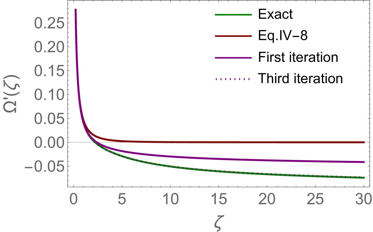
Figure 3: $\Omega^{\prime}\left(\zeta\right)$ versus $\zeta$ from Eq. (IV.14). $\Omega_{0}=1/4,\bar{\gamma}=0.63$. The first iteration at small $\zeta$ is given by $\mathcal{Z}\left(\zeta;{Eq.~(\ref{HOM75})}\right)\,+\,\Delta\mathcal{Z}\left(\zeta;{Eq.~(\ref{HOM120})}\right)$. The third iteration is calculated using Eq. (IV.18).

In Fig. 4 the resulting $\Omega\left(\zeta,l-l_{s}\right)$ is shown. One can see that $\Omega^{\prime}\left(\zeta,l-l_{s}\right)$ contribute only at rather small values of $\zeta$.

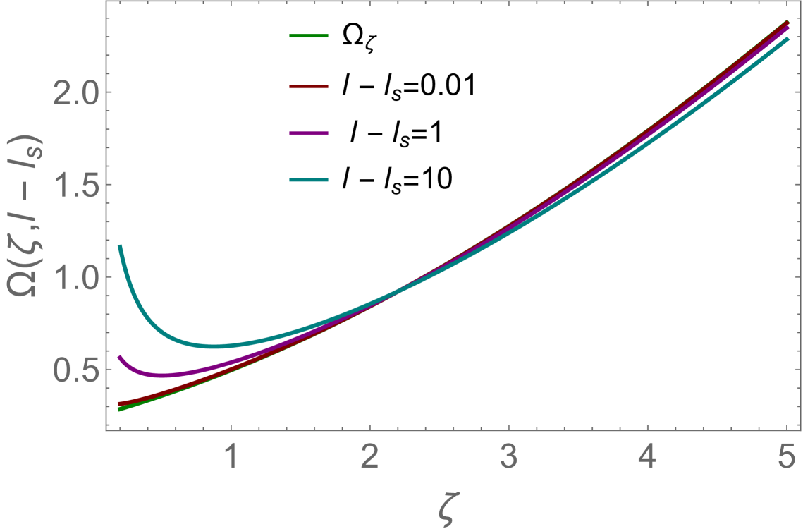
Figure 4: $\Omega\left(\zeta,l-l_{s}\right)$ versus $\zeta$ at fixed $l-l_{s}$. $\Omega=\Omega_{\zeta}^{(3)}+\Omega^{\prime}$ from Eq. (III.24) and Eq. (IV.13). $\Omega^{\prime}\left(\zeta,l-l_{s}\right)$ is the same as in Fig. 3.

V Homotopy approach: second iteration for the leading twist BFKL kernel

The next homotopy iteration stems from Eq. (IV.2):

$${\mathscr{H}}\left(p,\Omega^{(0)}+p\Omega^{(1)}\right)\,\,=\,\,\mathscr{L}[\Omega^{(0)}+p\,\Omega^{(1)}]\,+\,p\,\mathscr{N_{L}}[\Omega^{(0)}]\,\,=\,\,0$$ (V.1)

We need to account for the linear in $p$ terms in Eq. (IV.2). From Eq. (II.3)-Eq. (II.6) we obtain that Eq. (V.1) takes the form:

$$\dfrac{\partial^{2}\Omega^{(1)}\left(Y,l-l_{s}\right)}{\partial Y\,\partial l}\,\,=\,\,\left(1-e^{-\Omega^{(1)}\left(Y,l-l_{s}\right)}\right)\,\,e^{-\Omega^{(0)}\left(Y,l-l_{s}\right)}\,\,-\,\,\underbrace{\dfrac{\partial}{\partial\,l}\left(e^{\Omega^{(0)}\left(Y,l-l_{s}\right)}\mathscr{N_{L}}[\Omega^{(0)}]\right)}_{DH^{(0)}\left(Y,l-l_{s}\right)}$$ (V.2)

with $\Omega^{(0)}\left(\zeta,l-l_{s}\right)\equiv\,\Omega_{\zeta}^{(3)}\left(\zeta\right)+\Omega^{\prime}\left(\zeta,l-l_{s}\right)$.

In the derivation of Eq. (V.2) we assumed that $\left(\Omega^{(1)}\left(Y,l-l_{s}\right)\right)^{2}\,\ll\,\,\,\Omega^{(1)}\left(Y,l-l_{s}\right)$. The initial and boundary conditions for $\Omega^{(1)}\left(Y,l-l_{s}\right)$ takes the form:

$$\Omega^{(1)}\left(Y,l=l_{s}\right)\,=\,0;~~~~~\dfrac{\partial\Omega^{(1)}\left(Y,l-l_{s}\right)}{\partial\,l}\Big{|}_{l=l_{s}}\,=\,0;$$ (V.3)

In this section we calculate $\mathscr{N_{L}}[\Omega^{(0)}]$ for the simplified BFKL kernel. The BFKL kernel of Eq. (I.1) includes the summation over all twist contributions. In the simplified approach we restrict ourselves to the leading twist term only, which has the formLETU ; CLMS

$$\chi\left(\gamma\right)\,\,=\,\,\left\{\begin{array}[]{l}\,\,\,\,\,\,\,\frac{1}{\gamma}\,\,\,\,\,\,\,\,\,\mbox{for}\,\,\,\tau\,=\,rQ_{s}\,>\,1\,\,\,\,\,\mbox{summing}\left(\ln\left(rQ_{s}\right)\right)^{n};\\ \\ \,\,\,\frac{1}{1\,-\,\gamma}\,\,\,\,\,\mbox{for}\,\,\,\tau\,=\,rQ_{s}\,<\,1\,\,\,\,\,\mbox{summing}\left(\ln\left(1/(r\,\Lambda_{\rm QCD})\right)\right)^{n};\\ \end{array}\right.$$ (V.7)

instead of the full expression of Eq. (I.1).

For this simplified kernel Eq. (II.1) describe the contribution for $r_{1}\leq r$, while $N^{(0)}\left(Y,l^{\prime}\right)$ in the region $r^{\prime}>r$ in Eq. (I.1) contributes to $\mathscr{N_{L}}[N^{(0)}]$ which has the following form:

$$\mathscr{N_{L}}[\Omega^{(0)}]=\int\limits_{r_{1}\,>\,r}\,\frac{d^{2}r_{1}}{2\pi}\,K\left(r;r_{1},r_{2}\right)\exp\left(\,-\,\,\Omega^{(0)}\left(r_{1},Y;\boldsymbol{b}-\frac{1}{2}\,\boldsymbol{r}_{2}\right)\,-\,\Omega^{(0)}\left(r_{2},Y;\boldsymbol{b}-\frac{1}{2}\boldsymbol{r}_{1}\right)\right)$$ (V.8)

where $K\left(r;r_{1},r_{2}\right)$ is given by Eq. (I.2).

From Eq. (I.5) $\bar{\alpha}_{S}\left(r^{2}\right)\,\,=\,\,-\frac{4\,N_{c}}{b_{0}}\frac{1}{\xi}$. At $\xi=0$, $\bar{\alpha}_{S}\left(r^{2}\right)$ has a singularity (Landau pole). The behaviour of $\bar{\alpha}_{S}\left(r^{2}\right)$ for $\xi>0$ is the problem of non-perturbative QCD which has not been solved. We assume that this region of integration does not contribute in our integrals, reducing Eq. (V.9) to the expression:

$$\mathscr{N_{L}}[\Omega^{(0)}]=\int\limits_{r_{1}\,>\,r}^{1/\Lambda_{QCD}}\,\frac{d^{2}r_{1}}{2\pi}\,K\left(r;r_{1},r_{2}\right)\exp\left(\,-\,\,\Omega^{(0)}\left(r_{1},Y;\boldsymbol{b}-\frac{1}{2}\,\boldsymbol{r}_{2}\right)\,-\,\Omega^{(0)}\left(r_{2},Y;\boldsymbol{b}-\frac{1}{2}\boldsymbol{r}_{1}\right)\right)$$ (V.9)

Taking $\Omega^{(0)}=\Omega_{\zeta}^{(3)}+\Omega^{\prime}$, we can obtain the estimate for $\mathscr{N_{L}}[N^{(0)}]$ for the leading twist BFKL kernel, viz.:

$$\mathscr{N_{L}}[\Omega^{(0)}]=\frac{1}{2}\bar{\alpha}_{S}\left(r\right)\,e^{\xi}\!\!\!\!\!\int\limits^{0}_{\xi\geq-\xi_{s}}\!\!\!\!\!d\xi^{\prime}\,e^{-\xi^{\prime}}\exp\left(-\,\,2\,\left(\Omega_{\zeta}^{(3)}\left(\xi^{\prime}\right)+\Omega^{\prime}\left(Y,\xi^{\prime}\right)\,\right)\right)\,$$ (V.10)

Solving (numerically) Eq. (V.2) with the boundary and initial conditions of Eq. (V.3) we obtain $\Omega^{(1)}$. In Fig. 5 we plot $\Omega^{(0)}\left(\zeta,l-l_{s}\right)\equiv\Omega_{\zeta}\left(\zeta,l-l_{s}\right)$ and $\Omega^{(1)}\left(\zeta,l-l_{s}\right)$. One can see that $\Omega^{(1)}$ is much smaller that $\Omega^{(0)}$ as we expected.

However, the corrections to the scattering amplitude

$$\dfrac{N^{(1)}\left(Y,l-l_{s}\right)}{N^{(0)}\left(Y,l-l_{s}\right)}\,\,=\,\,\dfrac{\Omega^{(1)}\left(Y,l-l_{s}\right)\exp\left(-\Omega^{(0)}\left(Y,l-l_{s}\right)\right)}{1\,\,-\,\,\exp\left(-\Omega^{(0)}\left(Y,l-l_{s}\right)\right)}$$ (V.11)

turns out to be less that $5\%$ in the entire region of $Y$. Therefore, the first iteration of Eq. (IV.4) gives the solution to our problem with accuracy which is not worse than $5\%$ at small values of $Y$ ($Y\leq 5$). Note, that for $Y>5$ the accuracy is $<2\%$. For better accuracy we have to include the second iteration of Eq. (IV.2), which is linear in $p$.

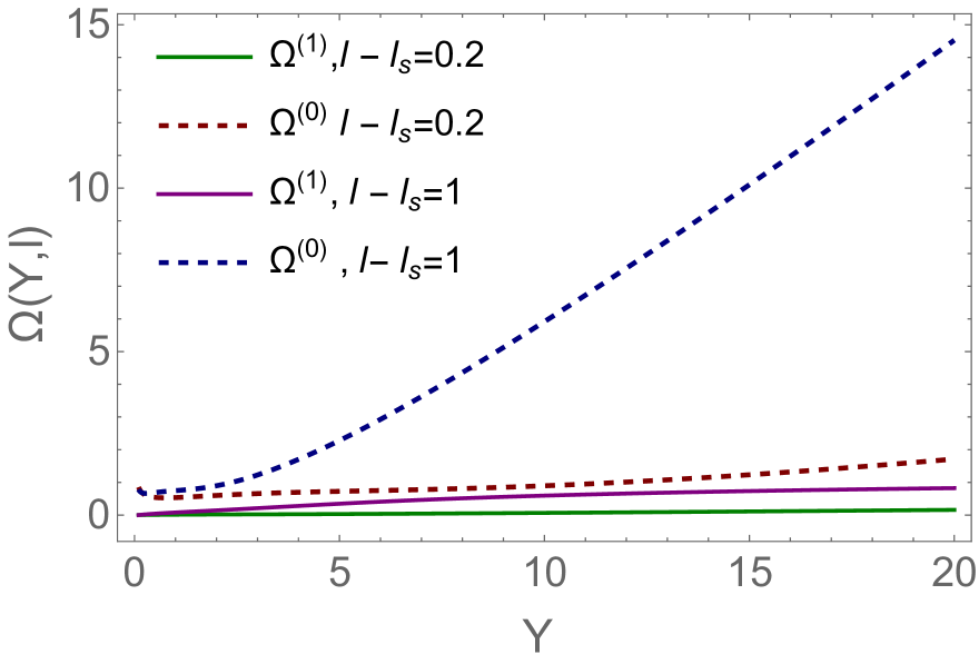
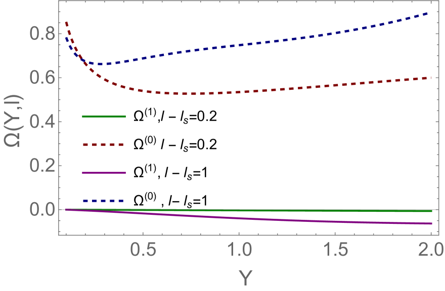
Fig. 5-a	Fig. 5-b

Figure 5: $\Omega^{(1)}\left(\zeta,l-l_{s}\right)$ versus $\zeta$ at fixed $l-l_{s}$ in comparison with $\Omega^{(0)}\left(\zeta.l-l_{s}\right)$. $\Omega_{0}=0.25,\bar{\gamma}=0.63$.

VI Homotopy approach: third iteration for the leading twist BFKL kernel

For rather small $l-l_{s}$ the second iteration gives a sizable contribution (about $5\%$) to the scattering amplitude (see Fig. 7-a). Bearing this in mind we have to estimate the third iteration to demonstrate that this iteration increases our accuracy.

The general equation for this iteration has the following form:

$${\mathscr{H}}\left(p,\Omega^{(0)}+p\,\Omega^{(1)}+p\,\Omega^{(2)}\right)\,\,=\,\,\mathscr{L}[\Omega^{(0)}+p\,\Omega^{(1)}+p\,\Omega^{(2)}]\,+\,p\,\mathscr{N_{L}}[\Omega^{(0)}+p\,\Omega^{(1)}]\,\,=\,\,0$$ (VI.1)

Eq. (VI.1) is the expansion of the general equation (see Eq. (IV.1) ) up to terms $\propto\,p^{2}$. From this equation we obtain:

$$\dfrac{\partial^{2}\Omega^{(2)}\left(Y,l-l_{s}\right)}{\partial Y\,\partial(l-l_{s})}\,\,=\,\,\Omega^{(2)}\left(Y,l-l_{s}\right)\,\,e^{-\Omega^{(0)}\left(Y,l-l_{s}\right)\,-\,\Omega^{(1)}\left(Y,l-l_{s}\right)}\,\,-\,\,\underbrace{\dfrac{\partial}{\partial\,(l-l_{s})}\left(e^{\Omega^{(0)}\left(Y,l-l_{s}\right)\,+\,\Omega^{(1)}\left(Y,l-l_{s}\right)}\mathscr{N_{L}}[\Omega^{(0)}\,+\,\Omega^{(1)}]\right)}_{DH^{(1)}\left(Y,l-l_{s}\right)}$$ (VI.2)

The initial and boundary conditions for $\Omega^{(2)}\left(Y,l-l_{s}\right)$ are the same as for $\Omega^{(1)}\left(Y,l-l_{s}\right)$ and they are given by Eq. (V.3). Repeating the same procedure as in the previous section we obtain that $\mathscr{N_{L}}[\Omega^{(0)}\,+\,\Omega^{(1)}]$ has the form:

$$\mathscr{N_{L}}[\Omega^{(0)}+\Omega^{(1)}] = \int\limits_{r_{1}\,>\,r}^{1/\Lambda_{QCD}}\,\frac{d^{2}r_{1}}{2\pi}\,K\left(r;r_{1},r_{2}\right)\exp\left(\,-\,\,\Omega^{(0)}\left(r_{1},Y;\boldsymbol{b}-\frac{1}{2}\,\boldsymbol{r}_{2}\right)\,-\,\Omega^{(0)}\left(r_{2},Y;\boldsymbol{b}-\frac{1}{2}\boldsymbol{r}_{1}\right)\right)$$ (VI.3)

$$\times ~\left(\Omega^{(1)}\left(r_{1},Y;\boldsymbol{b}-\frac{1}{2}\,\boldsymbol{r}_{2}\right)\,+\,\Omega^{(1)}\left(r_{2},Y;\boldsymbol{b}-\frac{1}{2}\boldsymbol{r}_{1}\right)\right)$$

where $K\left(r;r_{1},r_{2}\right)$ is given by Eq. (I.2).

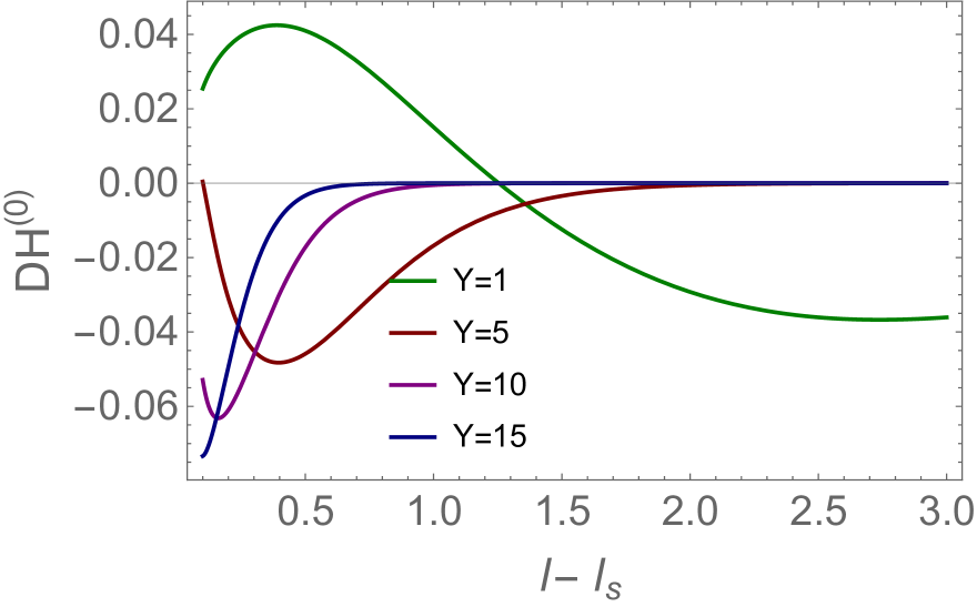
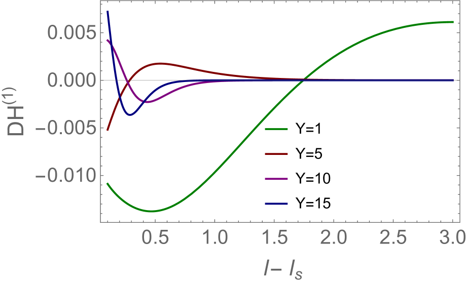
Fig. 6-a	Fig. 6-b

Figure 6: $DH^{(0)}\left(Y,l-l_{s}\right)$ (Fig. 6-a) and $DH^{(1)}\left(Y,l-l_{s}\right)$ (Fig. 6-b) from Eq. (V.2) and Eq. (VI.2) respectively as functions of $l-l_{s}$ at fixed $Y$. $\Omega_{0}=0.25,\bar{\gamma}=0.63$.

In Fig. 6 we plotted the nonhomogeneous terms of Eq. (V.2) and Eq. (VI.2). One can see that the nonhomogeneous term of Eq. (V.2) approximately is ten times larger than the same term on Eq. (VI.2). Therefore, without solving Eq. (VI.2) we can conclude that $\Omega^{(2)}$ will be suppressed by one order in comparison with $\Omega^{(1)}$. In Fig. 7 the solution to Eq. (VI.2) is plotted. One can see that the third iteration leads to small corrections in the entire region of $Y$ and $l-l_{s}$. Fig. 7-b shows that the contribution from the third interaction to the scattering amplitude turns out to be negligibly small ($\leq\,1\%$).

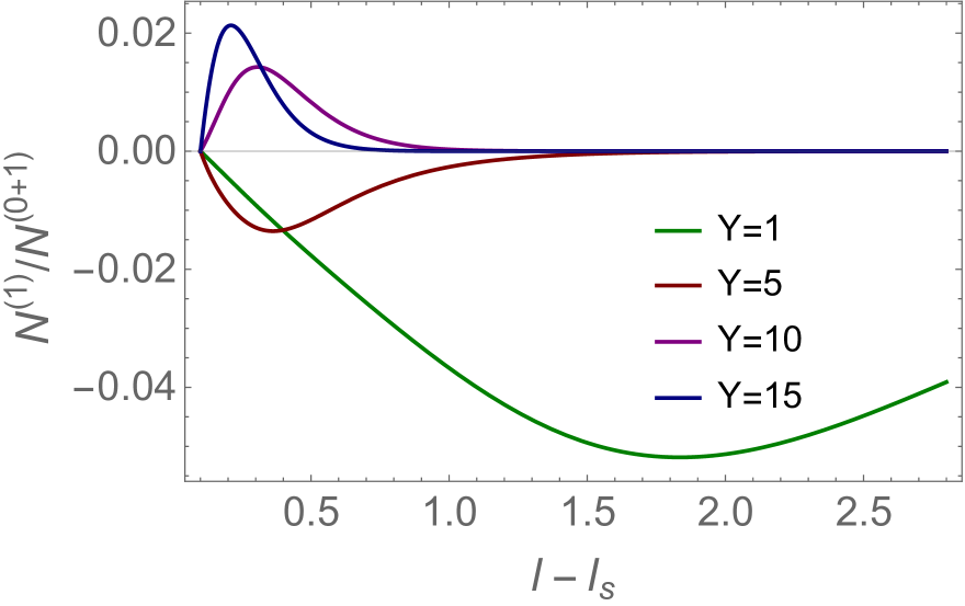
Fig. 7-a	Fig. 7-b

Figure 7: $\frac{N^{(1)}\left(Y,l-l_{s}\right)}{N^{(0+1)}\left(Y,l-l_{s}\right)}\,=\,\,\dfrac{\Omega^{(1)}\left(Y,l-l_{s}\right)\exp\left(-\Omega^{(0)}\left(Y,l-l_{s}\right)\right)}{1\,\,-\,\,\exp\left(-\Omega^{(0)}\left(Y,l-l_{s}\right)-\Omega^{(1)}\left(Y,l-l_{s}\right)\right)}$ (Fig. 7-a) and $\frac{N^{(2)}\left(Y,l-l_{s}\right)}{N^{(0+1)}\left(Y,l-l_{s}\right)}=\,\,\dfrac{\Omega^{(2)}\left(Y,l-l_{s}\right)\exp\left(-\Omega^{(0)}\left(Y,l-l_{s}\right)-\Omega^{(1)}\left(Y,l-l_{s}\right)\right)}{1\,\,-\,\,\exp\left(-\Omega^{(0)}\left(Y,l-l_{s}\right)-\Omega^{(1)}\left(Y,l-l_{s}\right)\right)}$ (Fig. 7-b) versus $l-l_{s}$ at fixed $Y$ (see Eq. (V.11)).

VII General BFKL kernel: second and third iterations

For the general BFKL kernel we have to take into account that (i) Eq. (II.6) does not describe the value of $\Omega$ for $r_{01}<r$; and (ii) for $r_{01}>r$ we have to use a more general kernel instead of $r^{2}/r^{4}_{02}$. Bearing these in mind we can rewrite equation for $\mathscr{N_{L}}[\Omega^{(0)}]$ in a general form:

$$\mathscr{N_{L}}[\Omega^{(0)}] = -\!\!\!\!\!\!\!\!\!\!\!\!\int\limits^{\xi}_{\begin{subarray}{l}r_{2}\,\gg\,1/Q_{s}(Y)\\ r_{1}\,\gg\,1/Q_{s}(Y)\end{subarray}}\!\!\!\!\!\!\!\!\!\!\!\!\frac{d^{2}r_{1}}{2\pi}\,\underbrace{K\left(r;r_{1},r_{2}\right)\exp\left(\,-\,\,\Omega^{(0)}\left(r_{1},Y\right)\,-\,\Omega^{(0)}\left(r_{2},Y\right)\right)-\bar{\alpha}_{S}(r_{1})\frac{1}{r^{2}_{1}}\exp\left(\,-\,\,\Omega^{(0)}\left(r_{1},Y\right)\,-\,\Omega^{(0)}\left(r,Y\right)\right)}_{\mbox{Difference between the general and model BFKL kernels in the region: $r_{1}<r$}}$$ (VII.1a)

$$- \!\!\!\!\!\!\!\!\!\!\!\!\int\limits^{\infty}_{\begin{subarray}{l}~~~~~~\xi\\ r_{2}\,\gg\,1/Q_{s}(Y)\\ r_{1}\,\gg\,1/Q_{s}(Y)\end{subarray}}\!\!\!\!\!\!\!\!\!\!\!\!\frac{d^{2}r_{1}}{2\pi}\,\underbrace{K\left(r;r_{1},r_{2}\right)\exp\left(\,-\,\,\Omega^{(0)}\left(r_{1},Y\right)\,-\,\Omega^{(0)}\left(r_{2},Y\right)\right)}_{\mbox{Contributions of the region: $r_{1}>r$}}$$

$$= -\!\!\!\!\!\!\!\!\!\!\!\!\int\limits^{1/\Lambda_{QCD}}_{\begin{subarray}{l}~~~~~~-\,\xi_{s}\\ r_{2}\,\gg\,1/Q_{s}(Y)\\ r_{1}\,\gg\,1/Q_{s}(Y)\end{subarray}}\!\!\!\!\!\!\frac{d^{2}r_{1}}{2\pi}\,K\left(r;r_{1},r_{2}\right)e^{\,-\,\Omega^{(0)}\left(r_{1},Y\right)\,-\,\Omega^{(0)}\left(r_{2},Y\right)}+\,\!\!\!\!\!\!\!\!\!\!\!\!\int\limits^{\xi}_{\begin{subarray}{l}~~~~~~\xi_{s}\\ r_{2}\,\gg\,1/Q_{s}(Y)\\ r_{1}\,\gg\,1/Q_{s}(Y)\end{subarray}}\!\!\!\underbrace{\bar{\alpha}_{S}(r_{1})\frac{dr^{2}_{1}}{r^{2}_{1}}e^{\,-\,\,\Omega^{(0)}\left(r_{1},Y\right)\,-\,\Omega^{(0)}\left(r,Y\right)}}_{\mbox{Contribution of the first iteration}}$$ (VII.1b)

In appendix A we discuss a simplification of Eq. (VII.1b). Using formulae of this appendix we reduce Eq. (V.2) for the second iteration to the form:

$$\dfrac{\partial^{2}\Omega^{(1)}\left(Y,l-l_{s}\right)}{\partial Y\,\partial l}\,\,=\,\,\left(2-e^{-\Omega^{(1)}\left(Y,l-l_{s}\right)}\right)\,\,e^{-\Omega^{(0)}\left(Y,l-l_{s}\right)}\,\,-\,\,\dfrac{\partial}{\partial\,l}\left(e^{\Omega^{(0)}\left(Y,l-l_{s}\right)}\mathscr{N^{\prime}_{L}}[\Omega^{(0)}]\right)$$ (VII.2)

However, it turns out that the formulae take the more economic form for the difference between Eq. (VII.1b) and Eq. (V.9) : $\Delta\mathscr{N_{L}}[\Omega^{(0)}]\,\,=\,\,\mathscr{N_{L}}[\Omega^{(0)},{Eq.~(\ref{SIG2})}]\,-\,\mathscr{N_{L}}[\Omega^{(0)},{Eq.~(\ref{SI31})}]$. Using the formulae of appendix A for $\Delta\mathscr{N_{L}}[\Omega^{(0)}]$ we have

$$\Delta\mathscr{N_{L}}[\Omega^{(0)}]\,\,=\,\,2\bar{\alpha}_{S}\left(r\right)\!\!\!\!\!\!\!\!\!\!\!\!\int\limits^{1/\Lambda_{QCD}}_{\begin{subarray}{l}~~~~~~-\,\xi_{s}\\ r_{2}\,\gg\,1/Q_{s}(Y)\\ r_{1}\,\gg\,1/Q_{s}(Y)\end{subarray}}\!\!\!\!\!\!\!\!\!\!\frac{dr^{2}_{1}}{r^{2}_{1}}\frac{rr_{1}\cos\left(\phi\right)-r^{2}_{1}}{r^{2}_{1}+r^{2}_{2}}\exp\left(\,-\,\,\Omega^{(0)}\left(r_{1},Y\right)\,-\,\Omega^{(0)}\left(r_{2},Y\right)\right)$$ (VII.3)

The solution to Eq. (VII.1b) for the general BFKL kernel is plotted in Fig. 8. One can see that the second iteration gives a small corrections for large $l-l_{s}$ ($l-l_{s}\geq 1$) . On the other hand these corrections are large for small $l-l_{s}$. For large $l-l_{s}$ we need to calculate the third iteration to obtain corrections of the order of few percents.

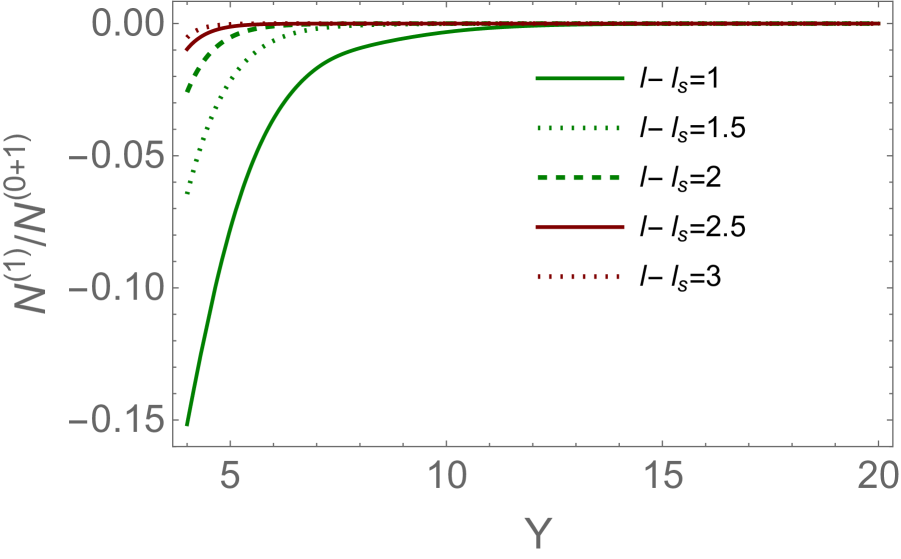
Fig. 8-a	Fig. 8-b

Figure 8: $\frac{N^{(1)}\left(Y,l-l_{s}\right)}{N^{(0+1)}\left(Y,l-l_{s}\right)}$ (see caption of Fig. 7) for the general BFKL kernel versus $Y$ at fixed $l-l_{s}$. $\Omega_{0}=0.25,\bar{\gamma}=0.63$.

For the third iteration we have Eq. (VI.2) with

$$\mathscr{N_{L}}[\Omega^{(0)}+\Omega^{(1)}] = \!\!\!\!\!\!\!\!\!\!\!\!\int\limits^{1/\Lambda_{QCD}}_{\begin{subarray}{l}r_{2}\,\gg\,1/Q_{s}(Y)\\ r_{1}\,\gg\,1/Q_{s}(Y)\end{subarray}}\,\!\!\!\!\!\!\!\!\!\!\!\!\frac{d^{2}r_{1}}{2\pi}\,K\left(r;r_{1},r_{2}\right)\exp\left(\,-\,\,\Omega^{(0)}\left(r_{1},Y;\boldsymbol{b}-\frac{1}{2}\,\boldsymbol{r}_{2}\right)\,-\,\Omega^{(0)}\left(r_{2},Y;\boldsymbol{b}-\frac{1}{2}\boldsymbol{r}_{1}\right)\right)$$ (VII.4)

$$\times ~\left(1\,\,-\,\,\exp\left(-\Omega^{(1)}\left(r_{1},Y;\boldsymbol{b}-\frac{1}{2}\,\boldsymbol{r}_{2}\right)\,-\,\Omega^{(1)}\left(r_{2},Y;\boldsymbol{b}-\frac{1}{2}\boldsymbol{r}_{1}\right)\right)\right)$$

Eq. (VII.4) is simplified in appendix B.

For small $l-l_{s}$ we have to calculate the fourth iteration. Facing such problem we decided to simplify our first iteration to obtain more transparent formulae for the higher ones. This is the goal of the next section.

VIII General BFKL kernel: alternative approach

In this section we are going to discuss an alternative approach for the general BFKL kernel which is based on the analytic of the BK equation solution (see Ref.LETU ) deeply in the saturation region.

VIII.1 Scattering amplitude at high energies for the general BFKL kernel:

The success of our approach actually stems from the simple solution of the nonlinear equation for the general BFKL kernel in high energy kinematic regionLETU . Indeed, at high energies (at $Y\gg 1$) the scattering amplitude approaches the unitarity limit: $N\left(r,Y;b\right)\xrightarrow{Y\gg 1}1$. Introducing $N\left(r,Y;b\right)\,=\,1\,\,-\,\,\Delta\left(r,Y;b\right)$ with $\Delta\left(r,Y;b\right)\,\ll\,1$, we can rewrite Eq. (I.1) in the form for the saturation region:

$$\dfrac{\partial\Delta\left(r,Y;b\right)}{\partial Y}\,\, = \,\,\int\,\frac{d^{2}r_{1}}{2\pi}\,K\left(r;r_{1},r_{2}\right)\Bigg{\{}-\Delta\left(r,Y;\boldsymbol{b}\right)\,+\,\Delta\left(r_{1},Y;\boldsymbol{b}-\frac{1}{2}\,\boldsymbol{r}_{2}\right)\,\Delta\left(r_{2},Y;\boldsymbol{b}-\frac{1}{2}\boldsymbol{r}_{1}\right)\Bigg{\}}$$ (VIII.1)

$$\xrightarrow{Y\gg 1} -\Delta\left(r,Y;\boldsymbol{b}\right)\!\!\!\!\!\!\!\!\!\!\!\!\underbrace{\int\limits_{\begin{subarray}{l}~r_{2}\,\gg\,1/Q_{s}(Y)\\ ~r_{1}\,\gg\,1/Q_{s}(Y)\end{subarray}}\!\!\!\!\!\!\!\!\!\!\!\!\frac{d^{2}r_{1}}{2\pi}\,K\left(r;r_{1},r_{2}\right)}_{\mbox{gluon reggeization}}$$

Introducing $\Delta\left(r,Y;\boldsymbol{b}\right)\,=\,\,\exp\left(-\Omega\left(r,Y;\boldsymbol{b}\right)\right)$ and taking the main logarithmic contribution for gluon reggeization we reduce Eq. (VIII.1) to the following equation:

$$\dfrac{\partial\Omega\left(r,Y;\boldsymbol{b}\right)}{\partial\,Y}\,\,=\,\,\int\limits^{r^{2}}_{1/Q^{2}_{s}}dr^{\prime 2}\frac{\bar{\alpha}_{S}\left(r^{\prime 2}\right)}{r^{\prime 2}}\,\,=\,\,l-l_{s}$$ (VIII.2)

In Eq. (VIII.2) we used the variable $l-l_{s}$ which has been introduced in Eq. (II.7). Eq. (VIII.2) can be rewritten as

$$\dfrac{\partial^{2}\Omega\left(r,Y;\boldsymbol{b}\right)}{\partial\,Y\,\partial(l-l_{s})}\,\,=1$$ (VIII.3)

which coincides with Eq. (III.1). Solution to this equation is equal to

$$\Omega\left(Y,l-l_{s}\right)\,\,=\,\,Y\,\left(l-l_{s}\right)+\tilde{\Omega}\left(Y,l-l_{s}\right);\,\,~~~\dfrac{\partial^{2}\tilde{\Omega}\left(r,Y;\boldsymbol{b}\right)}{\partial\,Y\,\partial l}\,\,=0\,\leftarrow\mbox{homogeneous equation}$$ (VIII.4)

Therefore, we demonstrated that at large values of $Y$ we obtain the same solution as for our nonlinear equation with the leading twist BFKL kernel. For matching the initial condition we use the solution of Eq. (III.3).

We suggest to use Eq. (VIII.3) as the first homotopy iteration and build the iterative procedure repeating all steps in finding the solution given in section III.

VIII.2 Second iteration

The second iteration to Eq. (VIII.1) we can write as follows:

$$\dfrac{\partial\Omega^{(1)}\left(r,Y;b\right)}{\partial Y}\,\,=\,\,(l-l_{s})-e^{\Omega^{(0)}\left(Y,l-l_{s}\right)}\int\,\frac{d^{2}r_{1}}{2\pi}\,K\left(r;r_{1},r_{2}\right)\exp\left(-\Omega^{(0)}\left(r_{1},Y;\boldsymbol{b}-\frac{1}{2}\,\boldsymbol{r}_{2}\right)\,-\Omega^{(0)}\left(r_{2},Y;\boldsymbol{b}-\frac{1}{2}\boldsymbol{r}_{1}\right)\right)$$ (VIII.5)

where $\Omega^{(0)}\left(Y,l-l_{s}\right)=Y(l-l_{s})\,-\,\bar{\gamma}\,\Omega_{0}\,\left(e^{-\frac{b_{0}}{4N_{c}}l}\,-\,e^{-\frac{b_{0}}{4N_{c}}l_{s}}\right)\,+\,\frac{1}{4\,\kappa}\left(e^{-\frac{b_{0}}{2N_{c}}l}\,-\,e^{-\frac{b_{0}}{2N_{c}}l_{s}}\right)\,\,+\,\,\Omega_{0}$ (see Eq. (III.3)).

Using Eq. (A.1) of appendix A we can rewrite Eq. (VIII.5) in the form:

$$\dfrac{\partial\Omega^{(1)}\left(r,Y;b\right)}{\partial Y}\,\,=\,\,(l-l_{s})-\bar{\alpha}_{S}\left(r^{2}\right)e^{\Omega^{(0)}\left(Y,l-l_{s}\right)}\!\!\!\!\!\!\!\!\!\!\!\!\int\limits^{1/\Lambda_{QCD}}_{\begin{subarray}{l}r_{2}\,\gg\,1/Q_{s}(Y)\\ r_{1}\,\gg\,1/Q_{s}(Y)\end{subarray}}\!\!\!\!\!\!\!\!\!\!\!\!\frac{d\phi dr_{1}^{2}}{2\pi}\,\Bigg{\{}\frac{r^{2}}{r^{2}_{1}\,(r^{2}_{1}+r^{2}_{2})}\,\,+\,\,\frac{1}{r^{2}_{1}}\frac{\ln\left(r^{2}_{2}/r^{2}_{1}\right)}{\ln r^{2}_{1}}\Bigg{\}}\exp\left(\,-\,\,\Omega^{(0)}\left(r_{1},Y\right)\,-\,\Omega^{(0)}\left(r_{2},Y\right)\right)$$ (VIII.6)

Hence,

$$\Omega^{(1)}\left(Y,l-l_{s}\right)\,\,=\,\,\Omega^{(0)}\left(Y,l-l_{s}\right)$$ (VIII.7)

$$-\int\limits^{Y}_{0}dY^{\prime}\bar{\alpha}_{S}\left(r^{2}\right)e^{\Omega^{(0)}\left(Y^{\prime},l-l_{s}\right)}\!\!\!\!\!\!\!\!\!\!\!\!\int\limits^{1/\Lambda_{QCD}}_{\begin{subarray}{l}r_{2}\,\gg\,1/Q_{s}(Y^{\prime})\\ r_{1}\,\gg\,1/Q_{s}(Y^{\prime})\end{subarray}}\!\!\!\!\!\!\!\!\!\!\!\!\frac{d\phi dr_{1}^{2}}{2\pi}\,\Bigg{\{}\frac{r^{2}}{r^{2}_{1}\,(r^{2}_{1}+r^{2}_{2})}\,\,+\,\,\frac{1}{r^{2}_{1}}\frac{\ln\left(r^{2}_{2}/r^{2}_{1}\right)}{\ln r^{2}_{1}}\Bigg{\}}\exp\left(\,-\,\,\Omega^{(0)}\left(r_{1},Y^{\prime}\right)\,-\,\Omega^{(0)}\left(r_{2},Y^{\prime}\right)\right)$$

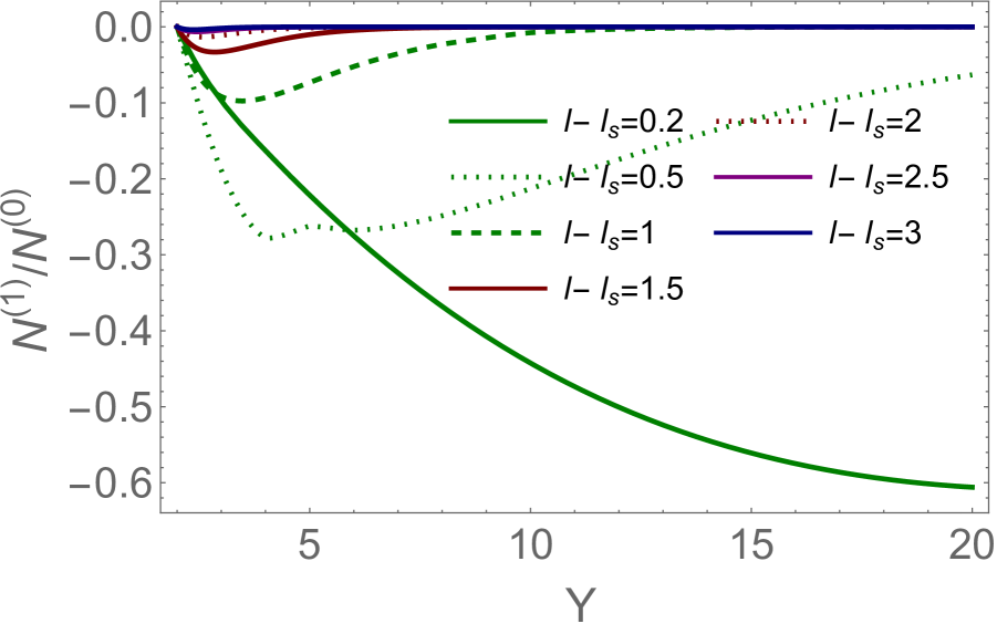
Fig. 9-a	Fig. 9-b

Figure 9: Fig. 9-a: The difference $\Omega^{(1)}\left(Y^{\prime},l-l_{s}\right)-\Omega^{(0)}\left(Y^{\prime},l-l_{s}\right)$ (see Eq. (VIII.8)) for the general BFKL kernel in the alternative approach versus $Y$ at fixed $l-l_{s}$. Fig. 9-b:$\frac{N^{(1)}\left(Y,l-l_{s}\right)}{N^{(0+1)}\left(Y,l-l_{s}\right)}$ (see caption of Fig. 7) for the general BFKL kernel in the alternative approach (see Eq. (VIII.8)) versus $Y$ at fixed $l-l_{s}$. $\Omega_{0}=0.25,\bar{\gamma}=0.63$.

As we have discussed in Eq. (VIII.5) we need to add to this equation the solution of homogeneous equation (see Eq. (VIII.5)) to satisfy the initial condition:

$$\Omega^{(1)}\left(Y,l-l_{s}=0\right)\,\,=\,\,\Omega^{(0)}\left(Y,l-l_{s}=0\right);~~~\frac{\partial}{\partial l}\Omega^{(1)}\left(Y,l-l_{s}\right)\Bigg{|}_{l=ls}\,\,=\,\,0$$

Hence, finally we have

$$\Omega^{(1)}\left(Y,l-l_{s}\right)\,\,=\,\,\Omega^{(1)}\left(Y,l-l_{s};{Eq.~(\ref{C6})}\right)$$ (VIII.8)

$$,\, -\,\,\Omega^{(1)}\left(Y,l-l_{s}=0;{Eq.~(\ref{C6})}\right)\,\,-\,\,\int\limits^{l}_{l_{s}}dl^{\prime}\frac{\partial\Omega^{(1)}\left(\frac{b_{0}\xi^{2}_{s}}{8\,N_{C}\,\kappa}e^{-\frac{b_{0}}{2\,N_{c}}l^{\prime}},l-l_{s};{Eq.~(\ref{C6})}\right)}{\partial l}\Bigg{|}_{l=l_{s}}$$

It is instructive to note that Eq. (VIII.7) gives an analytic solution for $\Omega^{(1)}$. From Fig. 9-a one can see that $\Omega^{(1)}-\Omega^{(0)}$ tuns out to be smaller than $\Omega^{(0)}$ at least for $l-l_{s}\geq 0.5$. Fig. 9 shows that the second iteration, which led to Eq. (VIII.7) , can be treated as corrections to $\Omega^{(0)}$. One can see that for $l-l_{s}>1$ the first iteration gives less that $10\%$ accuracy. Including the second iteration, which can be calculated analytically using Eq. (VIII.7), we can reach accuracy $\leq 1\%$. Therefore, we demonstrated that our procedure works.

VIII.3 Third iteration

Our second iteration was solution to the equation:

$$\frac{\partial\Delta^{(1)}\left(Y,l-l_{s}\right)}{\partial\,Y}\,\, = \,\,-\,\left(l-l_{s}\right)\,\Delta^{(1)}\left(Y,l-l_{s}\right)\,+\,\,\mathscr{N_{L}}[\Delta^{(0)}]$$

$$~\mbox{with}~~\mathscr{N_{L}}[\Delta^{(0)}]\, = \,\!\!\!\!\!\!\!\!\!\!\!\!\int\limits^{1/\Lambda_{QCD}}_{\begin{subarray}{l}r_{2}\,\gg\,1/Q_{s}(Y)\\ r_{1}\,\gg\,1/Q_{s}(Y)\end{subarray}}\!\!\!\!\!\!\!\!\!\!\!\!\frac{d^{2}r_{1}}{2\pi}\,K\left(r;r_{1},r_{2}\right)\exp\left(\,-\,\,\Omega^{(0)}\left(r_{1},Y\right)\,-\,\Omega^{(0)}\left(r_{2},Y\right)\right)$$ (VIII.9)

For the third iteration the equation takes the form:

$$\frac{\partial\Delta^{(2)}\left(Y,l-l_{s}\right)}{\partial\,Y}\,\, = \,\,-\,\left(l-l_{s}\right)\,\Delta^{(2)}\left(Y,l-l_{s}\right)\,+\,\,\mathscr{N_{L}}[\Delta^{(1)}]$$

$$~\mbox{with}~~\mathscr{N_{L}}[\Delta^{(1)}]\, = \,\!\!\!\!\!\!\!\!\!\!\!\!\int\limits^{1/\Lambda_{QCD}}_{\begin{subarray}{l}r_{2}\,\gg\,1/Q_{s}(Y)\\ r_{1}\,\gg\,1/Q_{s}(Y)\end{subarray}}\!\!\!\!\!\!\!\!\!\!\!\!\frac{d^{2}r_{1}}{2\pi}\,K\left(r;r_{1},r_{2}\right)\exp\left(\,-\,\,\Omega^{(1)}\left(r_{1},Y\right)\,-\,\Omega^{(1)}\left(r_{2},Y\right)\right)$$ (VIII.10)

One can see from Fig. 9-a that $\mathscr{N_{L}}[\Delta^{(1)}]\,<\,\mathscr{N_{L}}[\Delta^{(0)}]$ and, therefore, we can hope that the solution to this equation will lead to the better approximation for non-linear BK equation.

Introducing $\Delta^{(2)}\left(Y,l-l_{s}\right)\,\,=\,\,\exp\left(-\Omega^{(2)}\left(Y,l-l_{s}\right)\right)$ we can rewrite the solution to Eq. (VIII.3) as follows:

$$\Omega^{(2)}\left(Y,l-l_{s}\right)\,\,=\,\,\Omega^{(0)}\left(Y,l-l_{s}\right)$$ (VIII.11)

$$-\int\limits^{Y}_{0}dY^{\prime}\bar{\alpha}_{S}\left(r^{2}\right)e^{\Omega^{(0)}\left(Y^{\prime},l-l_{s}\right)}\!\!\!\!\!\!\!\!\!\!\!\!\int\limits^{1/\Lambda_{QCD}}_{\begin{subarray}{l}r_{2}\,\gg\,1/Q_{s}(Y^{\prime})\\ r_{1}\,\gg\,1/Q_{s}(Y^{\prime})\end{subarray}}\!\!\!\!\!\!\!\!\!\!\!\!\frac{d\phi dr_{1}^{2}}{2\pi}\,\Bigg{\{}\frac{r^{2}}{r^{2}_{1}\,(r^{2}_{1}+r^{2}_{2})}\,\,+\,\,\frac{1}{r^{2}_{1}}\frac{\ln\left(r^{2}_{2}/r^{2}_{1}\right)}{\ln r^{2}_{1}}\Bigg{\}}\exp\left(\,-\,\,\Omega^{(1)}\left(r_{1},Y^{\prime}\right)\,-\,\Omega^{(1)}\left(r_{2},Y^{\prime}\right)\right)$$

In Fig. 10 we plot the contribution of the third iteration. One can see that our procedure works and the third iteration improves the accuracy. However, for small values of $l-l_{s}\leq 1$ we certainly need to calculate the third iteration and, perhaps, the fourth iteration has to be included. In Fig. 11 and Fig. 12 we plotted the contribution of the third and fouth iterations. One can see that our procedure works.

For large values of $l-l_{s}\geq 1$ the third iteration leads to the scattering amplitude within several percent accuracy ($\leq 4\%$). At first sight it looks as we need more iterations than for the leading twist BFKL kernel. However, this is misleading impression since for the leading twist BFKL kernel we also need four iteration as it has been discussed in section III-C (see Fig. LABEL:omegazata).

IX Conclusions

Main results:

In the paper we developed the homotopy approach to the nonlinear Balitsky-Kovchegov equation for the running QCD coupling. As has been mentioned in the introduction our approach consists of two stages. The first one is the analytic solution to the nonlinear equation with a simplified BFKL kernel which has only the leading twist contributions. We found the analytic function for the scattering amplitude which satisfies the initial and boundary conditions. The second step was to find the corrections to this solution. The paper contains two investigation of these corrections: the detailed analysis of them in the simplified leading twist BFKL kernel and the development of the iteration procedure for the general BFKL kernel.

IX.1 Leading twist BFKL kernel

The substantial part of this paper is devoted to the investigation of the leading twist BFKL. The motivation for such approach is very simple: this kernel shows the largest difference between the fixed and running QCD coupling.

For the leading twist BFKL kernel we gave the detailed description of the corrections to our analytic solution. It is instructive to note that we calculate them using numerical estimates but the equation, that we solved numerically, depends only on analytic solution and did not bring any uncertainties. We demonstrated that the analytic first iteration leads the solution within 5% accuracy and calculating the second iteration we increased the accuracy to $\leq 1\%$.

Fig. 13 shows the scattering amplitude in the first and second iterations. One can see that we need to account for the second iteration for small $Y$ and $l-l_{s}$.

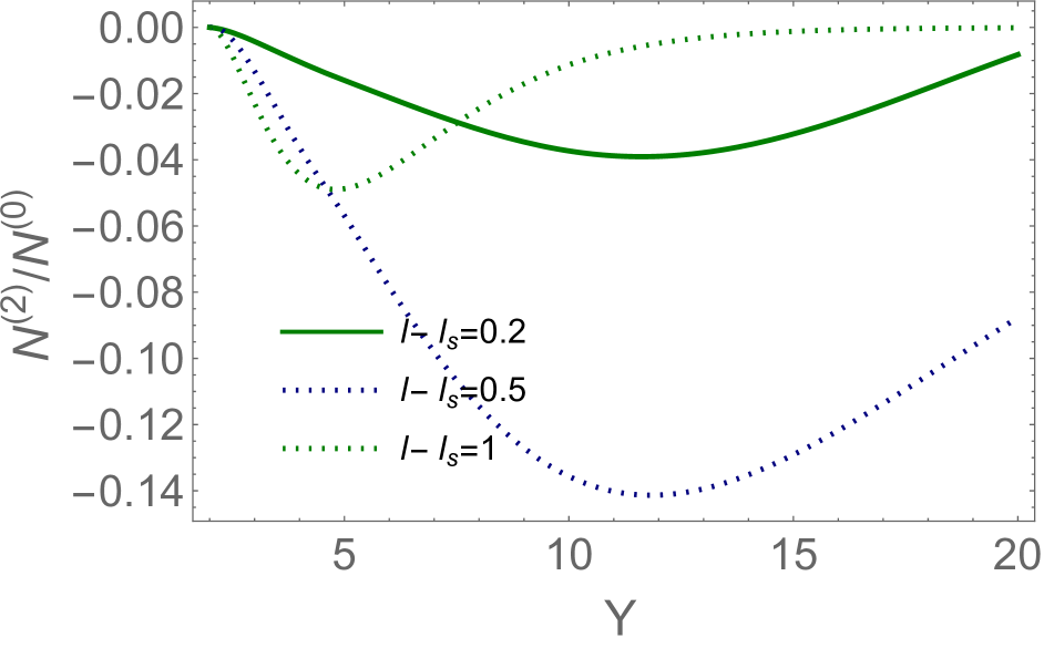
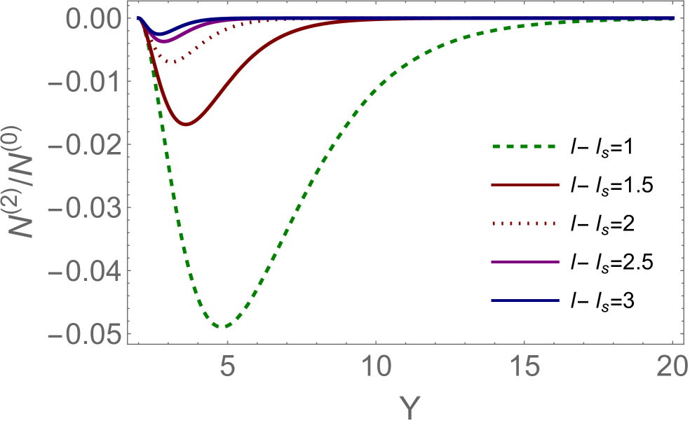
Fig. 10-a	Fig. 10-b

Figure 10: Fig. 10-a:$\frac{N^{(2)}\left(Y,l-l_{s}\right)}{N^{(0)}\left(Y,l-l_{s}\right)}$ (see caption of Fig. 7) for the general BFKL kernel in the alternative approach (see Eq. (VIII.11)) versus $Y$ at fixed small values of $l-l_{s}$. Fig. 10-b: The same at large values of $l-l_{s}$. $\Omega_{0}=0.25,\bar{\gamma}=0.63$.

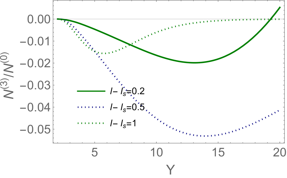
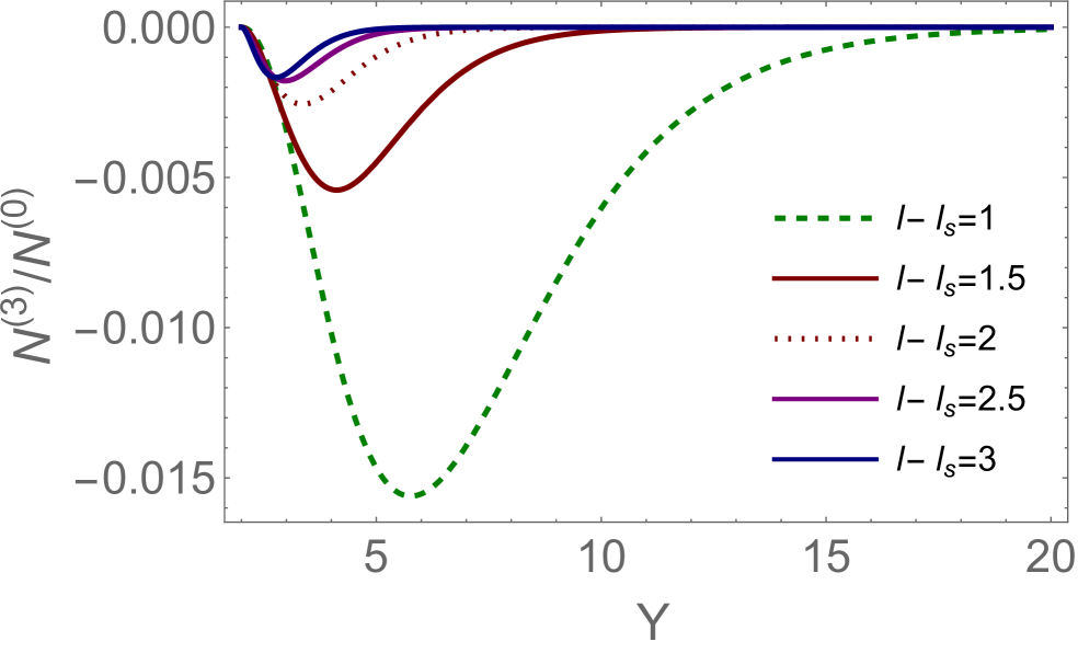
Fig. 11-a	Fig. 11-b

Figure 11: Fig. 11-a:$\frac{N^{(3)}\left(Y,l-l_{s}\right)}{N^{(0)}\left(Y,l-l_{s}\right)}$ (see caption of Fig. 7) for the general BFKL kernel in the alternative approach (see Eq. (VIII.11)) versus $Y$ at fixed small values of $l-l_{s}$. Fig. 11-b: The same at large values of $l-l_{s}$. $\Omega_{0}=0.25,\bar{\gamma}=0.63$.

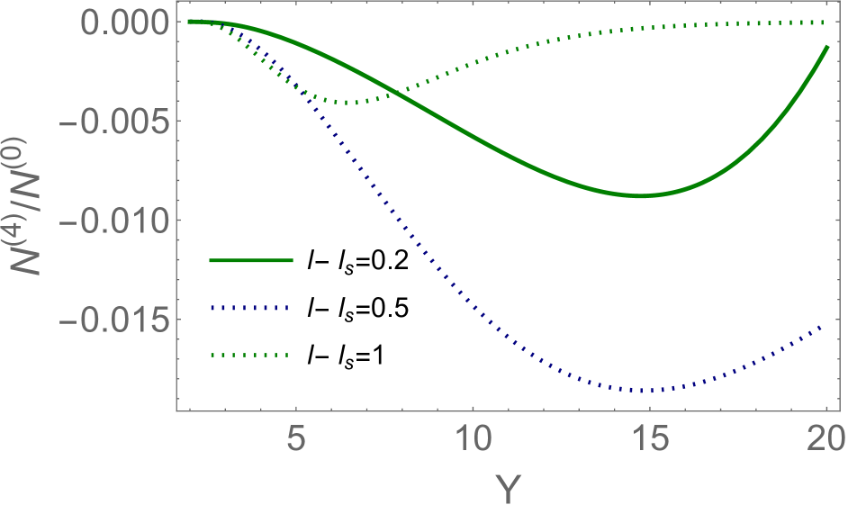
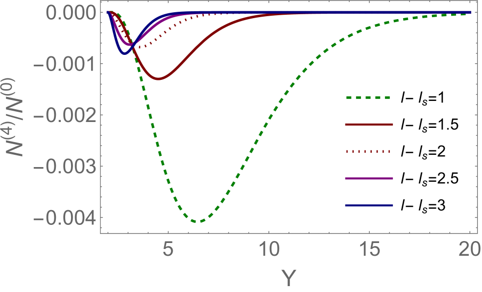
Fig. 12-a	Fig. 12-b

Figure 12: Fig. 12-a:$\frac{N^{(4)}\left(Y,l-l_{s}\right)}{N^{(0)}\left(Y,l-l_{s}\right)}$ (see caption of Fig. 7) for the general BFKL kernel in the alternative approach (see Eq. (VIII.11)) versus $Y$ at fixed small values of $l-l_{s}$. Fig. 12-b: The same at large values of $l-l_{s}$. $\Omega_{0}=0.25,\bar{\gamma}=0.63$.

$\mathbf{\zeta}$ scaling:

Eq. (VIII.5) as well as the solutions that have been discussed in sections I II-C and D, depend on one variable $\zeta=Y(l-l_{s})$ and therefore, show the $\zeta$ scaling behaviour. However this behaviour cannot satisfy the initial and boundary conditions and we have to add some violation of $\zeta$ scaling behaviour at low $l-l_{s}$. In Fig. 14 the $\Omega\left(\zeta,l-l_{s}\right)$ is plotted. One can see that (i) at large $\zeta$ and $l-l_{s}$ we have $\zeta$ scaling behaviour, but (ii) at low $\zeta$ and $l-l_{s}$ this behaviour is violated. Note, that this violation is larger at lower values of $\zeta$.

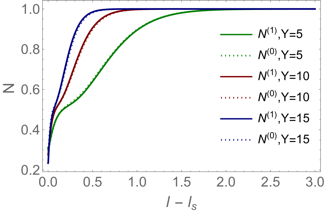
Figure 13: The scattering amplitude in the first and second iterations for the leading twist BFKL kernel.

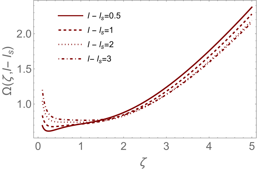
Fig. 14-a	Fig. 14-b

Figure 14: $\zeta=Y(l-l_{s})$ scaling behaviour for $\Omega\left(\zeta,l-l_{s}\right)=\,\Omega^{(0)}\left(Y,l-l_{s}\right)+\Omega^{(1)}\left(Y,l-l_{s}\right)+\Omega^{(2)}\left(Y,l-l_{s}\right)$.

Geometric scaling:

We wish to emphasize that we do not see any reason for the geometric scaling behaviour of $\Omega$ for the running QCD coupling. On the other hand, we have argued in section III-A (see Eq. (III.3) - Eq. (III.4)) that the geometric scaling behaviour could be in the vicinity of the saturation scale. Indeed, Fig. 15 show an approximate $z$-scaling behaviour in the limited region of $z$. In particular, one can see that the geometric scaling behaviour holds for small $l-l_{s}$ in rather wide region of $z=\xi_{s}+\xi$.

We wish to emphasize that the leading twist kernel demonstrates the most pronounced difference between the fixed QCD coupling with $z$ scaling and the running QCD coupling with $\zeta$ scaling behaviours.

Infrared cutoff:

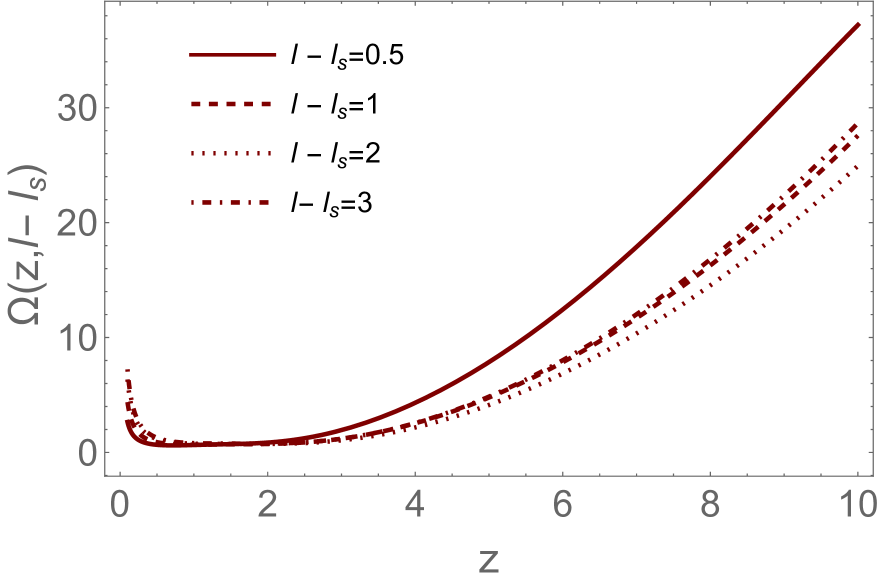
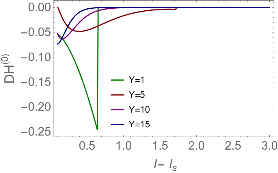
Fig. 15-a	Fig. 15-b

Figure 15: Fig. 15-a: $z=\xi_{s}+\xi$ scaling behaviour for $\Omega\left(\zeta,l-l_{s}\right)=\,\Omega^{(0)}\left(Y,l-l_{s}\right)+\Omega^{(1)}\left(Y,l-l_{s}\right)+\Omega^{(2)}\left(Y,l-l_{s}\right)$. Fig. 15-b: The nonhomogeneous term of Eq. (V.2) $DH^{(0)}\left(Y,l-l_{s}\right)$ versus $l-l_{s}$ at fixed $Y$ with the cut.

As we have discussed, we need to introduce an infrared cutoff to avoid the Landau pole in the running QCD coupling, since the nonperturbative methods of QCD have not solved the problem of long distance behaviour of the QCD coupling. In this paper we used this cutoff $r_{max}=1/\Lambda_{QCD}$. We demonstrated that the contributions of the distances of the order of $1/\Lambda_{QCD}$ in our equations can be neglected. We wish only to note that we can introduce any long distance behaviour of the running QCD coupling which could come from nonperturbative QCD or related phenomenology. In particular, there is a phenomenological reasonIFRCUT ; KOVCUT to cut long distances at $\bar{\alpha}_{S}\left(r_{max}\right)=\frac{1}{2}$. In Fig. 15-b one can see the nonhomogeneous term in Eq. (V.2) with this cut. Comparing this figure with Fig. 6-a we see that the difference in the infrared cut off change $DH^{(0)}\left(Y,l-l_{s}\right)$ only at small values of $Y$.

IX.2 Solution to the equation with the general BFKL kernel

The major part of this paper is devoted to the homotopy approach with the simplified, leading twist, BFKL kernel, since the main features of the running QCD coupling can be seen for this model in the clearest way. For the general BFKL kernel we demonstrated that our approach works well, considering two cases: (i) the first homotopy iteration is the nonlinear equation with the leading twist BFKL kernel; and (ii) the first iteration is the solution to the nonlinear BK equation at large values of $Y$. We demonstrated that for the general BFKL kernel our second approach gives the most economic way to describe large $Y$ region. Indeed, for large values of $Y$ we can use only the first iteration which has simple analytic solution. It is instructive to note that we can use the asymptotic solution of Eq. (VIII.5) in this region. However Fig. 17-a shows that the $\zeta$-scaling behaviour is strongly violated for the general BFKL kernel. Only for large values of $\zeta$ we see that $\Omega$ is independent of $l-l_{s}$. The $z$ scaling behaviour of the scattering amplitude (see Fig. 14) have the same patterns as for the leading twist BFKL kernel.

On the other hand for moderate value of $Y$ ($Y=1-7$) the simple approach we can trust only outside the vicinity of saturation scale at $l-l_{s}>1$. For smaller $l-l_{s}$ we have to take into account the second and, perhaps, even the third iterations. The behaviour of the scattering amplitude for the general BFKL kernel one can see in Fig. 17-b. This figure shows that corrections related to higher iterations are rather large.

We consider as one of the results of the paper that the leading twist BFKL kernel which models sufficiently well the nonlinear evolution for the freezed QCD coupling, does not work so well for the running QCD coupling. Indeed, we have seen that the solution to the general nonlinear equation does not reproduce the $zeta$ scaling, which is the inherent feature of the leading twist BFKL kernel.

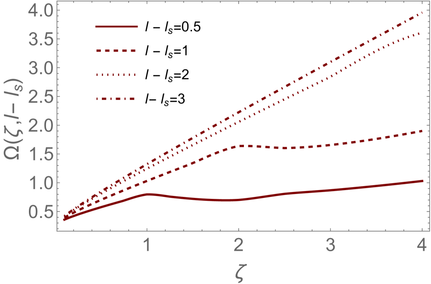
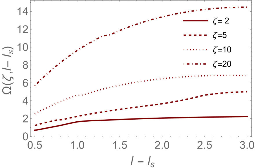
Fig. 16-a	Fig. 16-b

Figure 16: $\zeta=Y(l-l_{s})$ scaling behaviour for $\Omega\left(\zeta,l\right)=\,\Omega^{(0)}\left(Y,l-l_{s}\right)+\Omega^{(1)}\left(Y,l-l_{s}\right)$ for the general BFKL kernel

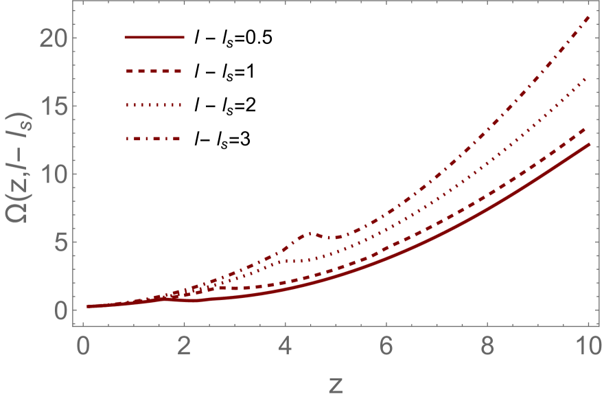
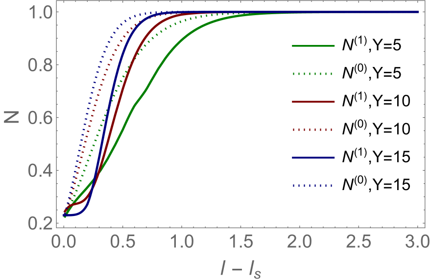
Fig. 17-a	Fig. 17-b

Figure 17: Fig. 17-a: $z=\xi_{s}+\xi$ scaling behaviour of $\Omega\left(\zeta,l-l_{s}\right)=\,\Omega^{(0)}\left(Y,l-l_{s}\right)+\Omega^{(1)}\left(Y,l-l_{s}\right)$ for the general BFKL kernel. Fig. 17-b: The scattering amplitude with the general BFKL kernel in the first and second iterations

IX.3 Concluding remarks:

We wish to recall that we consider the interaction of the dipole with the small size with the proton, which we model as the dipole with the size $R=1/\Lambda_{QCD}$. Our matching with perturbative QCD is determined by the solution of the linear BFKL equation at small dipole sizes. The initial condition for the BFKL equation is the Born approximation of perturbative QCD: the exchange of two gluons. In this paper we do not consider the initial condition of McLerran-Venugopalan type MV . This our reader has to bear in mind comparing our results with the numerical estimates in other papers (see, for example, Refs.KOLEB ; KOVCUT ; AAMS ). The influence of the McLerran-Venugopalan initial condition, which are correct for the dipole-nucleus scattering, we will consider in a separate paper.

We believe that the homotopy approach could be useful for treatment of the nonlinear dynamics in QCD and for accounting the effects related to the running QCD coupling.

X Acknowledgements

We thank our colleagues at Tel Aviv University and UTFSM for encouraging discussions. This research was supported by Fondecyt (Chile) grants No. 1231829 and 1231062. J.G. express his gratitude to the PhD scholarship USM-DP No. 029/2024 for the financial support. J.G. would also like to thank the organizers of the long-term workshop Hadrons and Hadron Interactions in QCD 2024 (HHIQCD 2024) at the Yukawa Institute for Theoretical Physics (YITP-T-24-02), Kyoto, Japan, where part of this work was completed.

Appendix A The general BFKL kernel: formulae for the second iteration

Using the identity :

$$\frac{1}{r_{1}^{2}\,r^{2}_{2}}\,=\,\frac{2}{r^{2}_{1}\,(r^{2}_{1}+r^{2}_{2})}$$

we can rewrite Eq. (VII.1b) in the form:

$$\mathscr{N_{L}}[\Omega^{(0)}] = \underbrace{-\bar{\alpha}_{S}\left(r^{2}\right)\!\!\!\!\!\!\!\!\!\!\!\!\int\limits^{1/\Lambda_{QCD}}_{\begin{subarray}{l}~~~~~~\xi_{s}\\ r_{2}\,\gg\,1/Q_{s}(Y)\\ r_{1}\,\gg\,1/Q_{s}(Y)\end{subarray}}\!\!\!\!\!\!\!\!\!\!\!\!\frac{d\phi dr^{2}}{2\pi}\,\Bigg{\{}\frac{r^{2}}{r^{2}_{1}\,(r^{2}_{1}+r^{2}_{2})}\,\,+\,\,\frac{1}{r^{2}_{1}}\frac{\ln\left(r^{2}_{2}/r^{2}_{1}\right)}{\ln r^{2}_{1}}\Bigg{\}}\exp\left(\,-\,\,\Omega^{(0)}\left(r_{1},Y\right)\,-\,\Omega^{(0)}\left(r_{2},Y\right)\right)}_{\mbox{$\mathscr{N^{\prime}_{L}}[\Omega^{(0)}]$}}$$ (A.1)

$$+ \underbrace{\int\limits^{\xi}_{\begin{subarray}{l}~~~~~~\xi_{s}\\ r_{2}\,\gg\,1/Q_{s}(Y)\\ r_{1}\,\gg\,1/Q_{s}(Y)\end{subarray}}\!\!\!\!\!\!\!\!\!\!\!\!\bar{\alpha}_{S}(r_{1}^{2})\frac{dr^{2}_{1}}{r^{2}_{1}}\exp\left(\,-\,\,\Omega^{(0)}\left(r_{1},Y\right)\,-\,\Omega^{(0)}\left(r,Y\right)\right)}_{\mbox{$\mathscr{N^{\prime\prime}_{L}}[\Omega^{(0)}]$}}$$

Note that $r^{2}_{2}=r^{2}+r^{2}_{1}-2r_{1}r\cos\phi$ and the identity used the symmetry between $r_{1}$ and $r_{2}$ in the integration.

The equation for $\Omega^{(1)}$ has the same form as Eq. (V.2). One can see that $\dfrac{\partial}{\partial\,l}\left(e^{\Omega^{(0)}\left(Y,l-l_{s}\right)}\mathscr{N_{L}}[\Omega^{(0)}]\right)$ from the second term in Eq. (A.1) can be found and it is equal to

$$\dfrac{\partial}{\partial\,l}\left(e^{\Omega^{(0)}\left(Y,l-l_{s}\right)}\mathscr{N^{\prime\prime}_{L}}[\Omega^{(0)}]\right)\,\,=\,\bar{\alpha}_{S}(\xi)\exp\left(-\,\Omega^{(0)}\left(r,Y\right)\right)\dfrac{d\xi}{dl}=\exp\left(-\,\Omega^{(0)}\left(r,Y\right)\right)$$ (A.2)

Using Eq. (A.2) we obtain Eq. (VII.2) for the second iteration.

Appendix B The general BFKL kernel: formulae for the third iteration

Eq. (VII.4) can be rewritten in the following form using Eq. (VII.1b):

$$\mathscr{N_{L}}[\Omega^{(0)}+\Omega^{(1)}] = -\bar{\alpha}_{S}\left(r^{2}\right)\!\!\!\!\!\!\!\!\!\!\!\!\int\limits^{1/\Lambda_{QCD}}_{\begin{subarray}{l}~~~~~~\xi_{s}\\ r_{2}\,\gg\,1/Q_{s}(Y)\\ r_{1}\,\gg\,1/Q_{s}(Y)\end{subarray}}\!\!\!\!\!\!\!\!\!\!\!\!\frac{d\phi dr^{2}}{2\pi}\,\Bigg{\{}\frac{r^{2}}{r^{2}_{1}\,(r^{2}_{1}+r^{2}_{2})}\,\,+\,\,\frac{1}{r^{2}_{1}}\frac{\ln\left(r^{2}_{2}/r^{2}_{1}\right)}{\ln r^{2}_{1}}\Bigg{\}}\exp\left(\,-\,\,\Omega^{(0)}\left(r_{1},Y\right)\,-\,\Omega^{(0)}\left(r_{2},Y\right)\right)$$ (B.1)

$$\times \left(1-\exp\left(-\Omega^{(1)}\left(Y,\frac{4}{3}\log\left(\frac{\ln(r^{2}_{2}}{\xi_{s}}\right)\right)-\Omega^{(1)}\left(Y,\frac{4}{3}\ln\left(\frac{\ln\left(r_{1}^{2}\right)}{\xi_{s}}\right)\right)\right)\right)$$

Note, that $\xi_{s}=\sqrt{\frac{8N_{c}}{b_{0}}\,\,\frac{\chi\left(\gamma_{cr}\right)}{1\,-\,\gamma_{cr}}\,Y}$ and $r^{2}_{2}=r^{2}+r^{2}_{1}-2r_{1}r\cos\phi$.

References

• (1) J.H. He, Comput. Methods Appl. Mech. Engrg. 173 (1999) 257.
• (2) J.H. He, Int. J. Nonlinear Mech. 35 (2000) 37.
• (3) I. Balitsky, Phys. Rev. D60, 014020 (1999); Y. V. Kovchegov, Phys. Rev. D60, 034008 (1999).
• (4) C. Contreras, E. Levin and R. Meneses, Phys. Rev. D 107 (2023) no.9, 094030 doi:10.1103/PhysRevD.107.094030 [arXiv:2302.10497 [hep-ph]].
• (5) Y. V. Kovchegov and E. Levin, Nucl. Phys. B 577 (2000) 221.
• (6) C. Contreras, J. Garrido, E. Levin and R. Meneses, Phys. Rev. D 110 (2024) 054045
• (7) V. S. Fadin, E. A. Kuraev and L. N. Lipatov, Phys. Lett. B60, 50 (1975);    E. A. Kuraev, L. N. Lipatov and V. S. Fadin, Sov. Phys. JETP 45, 199 (1977), [Zh. Eksp. Teor. Fiz.72,377(1977)];    I. I. Balitsky and L. N. Lipatov, Sov. J. Nucl. Phys. 28, 822 (1978), [Yad. Fiz.28,1597(1978)].
• (8) B. Diaz Saez and E. Levin, Nucl. Phys. A 870-871 (2011), 83-93 doi:10.1016/j.nuclphysa.2011.09.003 [arXiv:1106.6257 [hep-ph]].
• (9) I.Balitsky, Phys. Rev. D 75 (2007) 014001
• (10) Y.V. Kovchegov and H. Weigert, Nucl. Phys. A 784 (2007), 789 (2007) 260.
• (11) J. L. Albacete and Y. V. Kovchegov, Phys. Rev. D 75, 125021 (2007) doi:10.1103/PhysRevD.75.125021 [arXiv:0704.0612 [hep-ph]].
• (12) L. V. Gribov, E. M. Levin and M. G. Ryskin, Phys. Rept.  100, 1 (1983).
• (13) A. H. Mueller and D. N. Triantafyllopoulos, Nucl. Phys.B640 (2002) 331 [arXiv:hep-ph/0205167];  D. N. Triantafyllopoulos, Nucl. Phys.B648 (2003) 293 [arXiv:hep-ph/0209121].
• (14) S. Munier and R. B. Peschanski, Phys. Rev.  D 70 (2004) 077503 [arXiv:hep-ph/0401215];   Phys. Rev.  D 69 (2004) 034008 [arXiv:hep-ph/0310357];   Phys. Rev. Lett.  91 (2003) 232001 [arXiv:hep-ph/0309177].
• (15) Yuri V. Kovchegov and Eugene Levin, “ Quantum Chromodynamics at High Energies", Cambridge Monographs on Particle Physics, Nuclear Physics and Cosmology, Cambridge University Press, 2012 .
• (16) E. Iancu, K. Itakura, L. McLerran, Nucl. Phys.  A708 (2002) 327-352. [hep-ph/0203137]
• (17) K. J. Golec-Biernat and A. M. Stasto, Nucl. Phys. B 668 (2003), 345-363 [arXiv:hep-ph/0306279 [hep-ph]].
• (18) J. Berger and A. Stasto, Phys. Rev. D 83 (2011), 034015 [arXiv:1010.0671 [hep-ph]].
• (19) L. N. Lipatov, Sov. Phys. JETP 63, 904 (1986) [Zh. Eksp. Teor. Fiz.  90, 1536 (1986)].
• (20) L. N. Lipatov, Phys. Rept.  286 (1997) 131.
• (21) E. Levin and K. Tuchin, Nucl. Phys. B 573, 833 (2000) [hep-ph/9908317];    Nucl. Phys. A 691, 779 (2001) [hep-ph/0012167]; 693, 787 (2001) [hep-ph/0101275].
• (22) C. Contreras, E. Levin, R. Meneses and M. Sanhueza, Eur. Phys. J. C 80, no.11, 1029 (2020) doi:10.1140/epjc/s10052-020-08580-w [arXiv:2007.06214 [hep-ph]].
• (23) A.H.  Mueller, Nucl.Phys. B643 (2002) 501
• (24) I. Gradstein and I. Ryzhik, “ Table of Integrals, Series, and Products”, Fifth Edition, Academic Press, London, 1994.
• (25) Andrei D. Polyanin and Valentin F. Zaitsev, “ Handbook of nonlinear Partial Differential Equations", Chapman $\&$ Hall/CRC, 2004.
• (26) S. Godfrey and N. Isgur, Phys. Rev. D 32, 189-231 (1985) doi:10.1103/PhysRevD.32.189
• (27) L. McLerran and R. Venugopalan, Phys. Rev. D49 (1994) 2233, Phys. Rev. D49 (1994), 3352; D50 (1994) 2225; D59 (1999) 09400.
• (28) Javier L. Albacete, Néstor Armesto, Néstor,José Guilherme Milhano and Carlos A.Salgado, Phys. Rev. D 80 (2009) 034031, [arXiv:0902.1112 [hep-ph]], and reference therein.